1

DRAFT

SCALLOP ACL FLOWCHART DISCUSSION PAPER

June 1May 20, 2016

Version 2

Version 2 – Updated with Scallop Committee Input

2

Intentionally Blank

3

1.0 CONTENTS

1.1 TABLE OF CONTENTS 1.0 Contents .............................................................................................................................. 3

1.1 Table of Contents ............................................................................................................ 3

1.2 List of Tables .................................................................................................................. 4

1.3 List of Figures ................................................................................................................. 4

2.0 Draft Problem Statement..................................................................................................... 5

3.0 Background ......................................................................................................................... 5

3.1 Amendment 11 ................................................................................................................ 5

3.2 Amendment 15 ................................................................................................................ 5

3.3 Performance to Date ....................................................................................................... 9

4.0 Draft objectives ................................................................................................................. 14

5.0 Draft measures .................................................................................................................. 15

5.1 Modifications to Scallop ACL Flowchart ..................................................................... 15

5.1.1 No Action .................................................................................................................. 15

5.1.2 Modify ACL Flowchart ............................................................................................ 15

5.1.2.1 Option A: Consider a management uncertainty buffer for the LAGC fishery .. 15 5.1.2.2 Option B: Consider modifying ACL structure to incorporate spatial management into catch limits based on projected landing estimates ............................ 18 5.1.2.3 Comparison of ACL flowchart options .............................................................. 21

5.2 Other Potential Measures .............................................................................................. 23

5.2.1.1 Consider modifying how the observer set-aside is removed from the ACL flowchart 23

6.0 PDT discussion and Recommendations ............................................................................ 25

4

1.2 LIST OF TABLES Table 1 - Relevant Terms and Definitions (also see A15 p.69). Values updated from SARC 59 (2014). ............................................................................................................................................. 6 Table 2 - Performance of ACL management to date. FY 2015 landings (actual mt, lb) are estimates. ......................................................................................................................................... 9 Table 3 – Comparison of LAGC allocations when applying 5%, 10%, and 20% management uncertainty buffers and the mt difference between what the LAGC IFQ sub-ACL would have been if a management buffer were in place and actual landing. A positive value in these columns indicates that landings for the FY were less than the ACL with a management buffer applied. Values in metric tons. ................................................................................................................... 16 Table 4 - Comparison of LAGC allocations when applying a spatially explicit approach and the mt difference between what the LAGC IFQ sub-ACL would have been using a spatially explicit approach and actual landing. A negative value in indicates that landings for the FY were greater than the ACL using a spatially explicit approach. Values in metric tons. .................................... 18 Table 5 - Comparison of LA allocations when applying a spatially explicit approach and the mt difference between what the LA sub-ACL would have been using a spatially explicit approach and actual landing. A negative value in indicates that landings for the FY were greater than the Option B sub-ACT “spatially explicit approach.” Values in metric tons. .................................... 19 Table 6 - Comparison of LAGC IFQ allocation values under status quo, Option A, and Option B. Values in metric tons. The sub-ACL and sub-ACT columns are equal, and shown for comparison purposes. ....................................................................................................................................... 21 Table 7 - Comparison of LA ACT allocation values under status quo, Option A, and Option B. Values in metric tons. ................................................................................................................... 21 Table 9 – Comparison of approaches to setting the observer set-asides, including actual catch by fishing year.................................................................................................................................... 24 Table 10 - Actual observer landings as a percentage of status quo (1% of ACL) and other potential options. ........................................................................................................................... 25

1.3 LIST OF FIGURES Figure 1 - Current OFL/ABC/ACL flowchart process ................................................................... 7 Figure 2 - Current method used to calculate LA open area DAS ................................................... 8 Figure 3 - OFL, ABC/ACL, ACT, and Projected Landing values for FY2011 - 2015. ACT values are approximate. Note the increase in the OFL and the slight decrease in projected landing in FY2016. .................................................................................................................................... 11 Figure 4 - Performance of LAGC IFQ landings relative to quotas, FY2011- FY2015. ............... 12 Figure 5 - Performance of limited access landings relative to allocations, FY2011 – FY 2015. . 13 Figure 6 – Option A considers a management uncertainty buffer for the LAGC component of the fishery. .......................................................................................................................................... 17 Figure 7 – Option B considers modifying the ACL structure to incorporate spatial management into catch limits based on projected landings estimates. There would be no changes to the process for setting the ABC/ACL and OFL. ................................................................................. 20 Figure 8 - Comparison of approaches to setting the observer set-aside, including actual catch by fishing year. Note that the FY2015 bar for actual catch is hatched because data is preliminary. 24

5

2.0 DRAFT PROBLEM STATEMENT The current ACL structure and fishery allocations in the Scallop FMP are not spatially explicit. Annual catch limits (ACLs) in the scallop fishery are based on scallop biomass in all areas, including closed areas, while. pProjected landings are limited to areas that are open to the fishery in a given year. This can be problematic because the overall scallop management program is an area based system that is spatially explicit. The disconnect between the catch limits and projected landings is more of an issue when higher levels of total biomass are in closed areas and not available to the fishery.

Additionally, measures adopted during and since Amendment 15 have introduced the potential for management uncertainty. The scallop PDT identified several sources of management uncertainty in A15. These include mortality from carry-over allowances, vessel upgrades, ability of the FMP to monitor and enforce all catch, and changes in fishing behavior that may increase landings above projected values. An example of a change made through A15 is that the LAGC IFQ component is now allowed to carryover up to 15% of allocated quota from one fishing year to the next.

3.0 BACKGROUND

3.1 AMENDMENT 11 Amendment 11 implemented limited entry for three LAGC permit categories: LAGC IFQ, LAGC NGOM, and LAGC Incidental. Separate TACs were developed for the NGOM and Incidental permits, but the IFQ TAC is part of the scallop fishery TAC the limited access vessels work under as well.

Staff will insert some background about the allocation decisions and rationale from A11

3.2 AMENDMENT 15 Amendment 15 (A15) was developed to bring the Scallop FMP in compliance with new requirements to end and prevent overfishing using annual catch limits (ACLs) and accountability measures (AMs) (reauthorization of the Magnuson Stevens Act in 2007). To do so, A15 included several terms and definitions which are relevant to the ACL flowchart (Table 1). The scallop fishery uses an overall approach of OFL > ABC = ACL > ACT.

For the Scallop FMP, annual catch limits are based on scallop biomass that is exploitable to survey gear (40mm+). The biomass from all areas, including closed areas, is included in the OFL, ABC, and ACLs for the fishery. Therefore, the allocation split from Amendment 11 is still carried over under this FMP, but it is made at the ACL level, not the projected catch level. The LA fishery receives 94.5% of the ACL and the LAGC IFQ fishery receives 5.5% of the ACL, after set-asides and discard estimates have been removed. Amendment 15 was explicit that the allocation decision should be made at the ACL level, before buffers for management uncertainty are applied. Therefore, the allocation split occurs at the ACL level, and no longer at the projected catch level, as it was under Amendment 11.

6

Figure 1 the current ACL structure, while Figure 2 depicts how allocations are derived from projected landings using LA open area DAS as an example. As the ACL is not spatially explicit, when projected landing are below the ACL and ACT actual allocations may correspond to lower F rates for the fishery.

Table 1 - Relevant Terms and Definitions (also see A15 p.69). Values updated from SARC 59 (2014).

Term Definition Value for Scallop FMP

Maximum Sustainable Yield (MSY)

Largest long-term average catch or yield. Results from applying Fmsy.

Fmsy = Fmax = 0.48

Status Determination Criteria (SDC)

Quantifiable factors used to determine if overfishing has occurred and if stock is overfished

SDC for Scallop FMP is Fthreshold of 0.48 and Bthreshold of 48,240 mt, meats.

Maximum Fishing Mortality Threshold (MFMT)

Level of fishing mortality above which overfishing is occurring.

MFMT = Fthreshold = 0.48

Minimum Sustainable Stock Threshold (MSST)

Level of biomass below which stock is considered overfished.

MSST = Bthreshold = ½ Bmsy = 48,240 (mt, meats)

Overfishing Limit (OFL)

Annual amount of catch above which overfishing is occurring, results from applying MFMT or Fthreshold to stock abundance.

OFL

Optimum Yield (OY)

MSY reduced by relevant social, economic, and ecological factors. OY = ACL

Acceptable Biological Catch (ABC)

Maximum catch recommended for harvest. Can never exceed OFL and should consider scientific uncertainty.

ABC set 25% lower than OFL (SSC recommendation)

Annual Catch Limit (ACL)

Annual amount of catch over which accountability measures triggered. ACL can equal but never exceed ABC

ABC = ACL

Sector ACL Overall ACL can be divided into sub-ACLs if differences in degree of management uncertainty.

Scallop FMP will have 2 sub-ACLs: one for limited access (LA) and one for limited access general category fishery (LAGC). ACL = LA ACL + LAGC ACL

Annual Catch Target (ACT)

Amount of annual catch that is the management target and accounts for management uncertainty.

Scallop FMP will have 2 ACTs: LA ACT will be set at F level with 25% chance of exceeding ABC and LAGC ACT will be set equal to LAGC sub-ACL.

7

Figure 1 - Current OFL/ABC/ACL flowchart process

8

Figure 2 - Current method used to calculate LA open area DAS

9

3.3 PERFORMANCE TO DATE Table 2 - Performance of ACL management to date. FY 2015 landings (actual mt, lb) are estimates.

% of Total Allocated

% Difference (allocated vs actual)

% of Total Actual

mt lb mt lbOFL 32,387 71,401,113 81.88%ABC/ACL 27,269 60,117,854 97.24%Total Projected Landings 23,723 52,300,000 26,518 58,461,465 112%incidental 23 50,000 0.10% 18 38,700 77% 0.07%RSA 567 1,250,000 2.39% 553 1,218,781 98% 2.08%OBS 273 601,170 1.15% 104 228,370 38% 0.39%IFQ 1,452 3,201,880 6.12% 1,382 3,046,245 95% 5.21%LA ACT 21,431 47,247,267 90.34% 24,462 53,929,369 114% 92.25%LA ACL 24,954 55,014,153 24,462 53,929,369OFL 34,382 75,799,335 75.33%ABC/ACL 28,961 63,848,076 89.43%Total Projected Landings 25,945 57,200,000 25,900 57,098,684 100%incidental 23 50,000 0.09% 28 61,869 124% 0.11%RSA 567 1,250,000 2.19% 529 1,167,316 93% 2.04%OBS 290 638,470 1.12% 120 263,700 41% 0.46%IFQ 1,544 3,405,000 5.95% 1,511 3,331,284 98% 5.83%LA ACT 23,546 51,910,044 90.75% 23,711 52,274,515 101% 91.55%LA ACL 26,537 58,503,960OFL 31,555 69,566,867 57.22%ABC/ACL 21,004 46,305,894 85.97%Total Projected Landings 17,335 38,216,741 18,056 39,807,589 104%incidental 23 50,000 0.13% 21 47,337 95% 0.12%RSA 567 1,250,000 3.27% 553 1,218,204 97% 3.06%OBS 210 463,059 1.21% 174 384,545 83% 0.97%IFQ 1,111 2,449,856 6.41% 1,095 2,414,256 99% 6.06%LA ACT 15,324 33,783,637 88.40% 16,213 35,743,247 106% 89.79%LA ACL 19,093 42,092,979 16,213 35,743,247OFL 30,419 67,062,415 0 47.75%ABC/ACL 20,782 45,816,467 0 69.89%Total Projected Landings 17,327 38,463,656 14,524 32,020,980 83%incidental 23 50,000 0.13% 19 42,107 84% 0.13%RSA 567 1,250,000 3.27% 433 954,011 76% 2.98%OBS 208 458,562 1.20% 177 390,579 85% 1.22%IFQ 1,099 2,423,145 6.34% 948 2,089,589 86% 6.53%LA ACT 15,567 34,319,360 89.84% 12,948 28,544,694 83% 89.14%LA ACL 18,885 41,634,305 12,948 28,544,694

Allocated Actual

2011

2012

2013

2014

10

% of Total Allocated

% Difference (allocated vs actual)

% of Total Actual

mt lb mt lbOFL 38,061 83,910,142ABC/ACL 25,352 55,891,593Total Projected Landings 21,500 47,400,000incidental 23 50,000 0.11%RSA 567 1,250,021 2.64%OBS 254 559,974 1.18% 220 484,955 87%IFQ 1,348 2,971,831 6.27% 1,161 2,559,595 86%LA ACT 19,331 42,617,560 89.91% 14,317 31,564,479 74%LA ACL 23,161 51,061,265OFL 68,418 150,835,870ABC/ACL 37,852 83,449,375Total Projected Landings 21,288 46,932,006incidental 23 50,000 0.11%RSA 567 1,250,000 2.66%OBS 379 835,552 1.78%IFQ 2,029 4,473,180 9.53%LA ACT 18,290 40,322,555 85.92%LA ACL 34,855 76,842,135

2016

2015

Allocated Actual

11

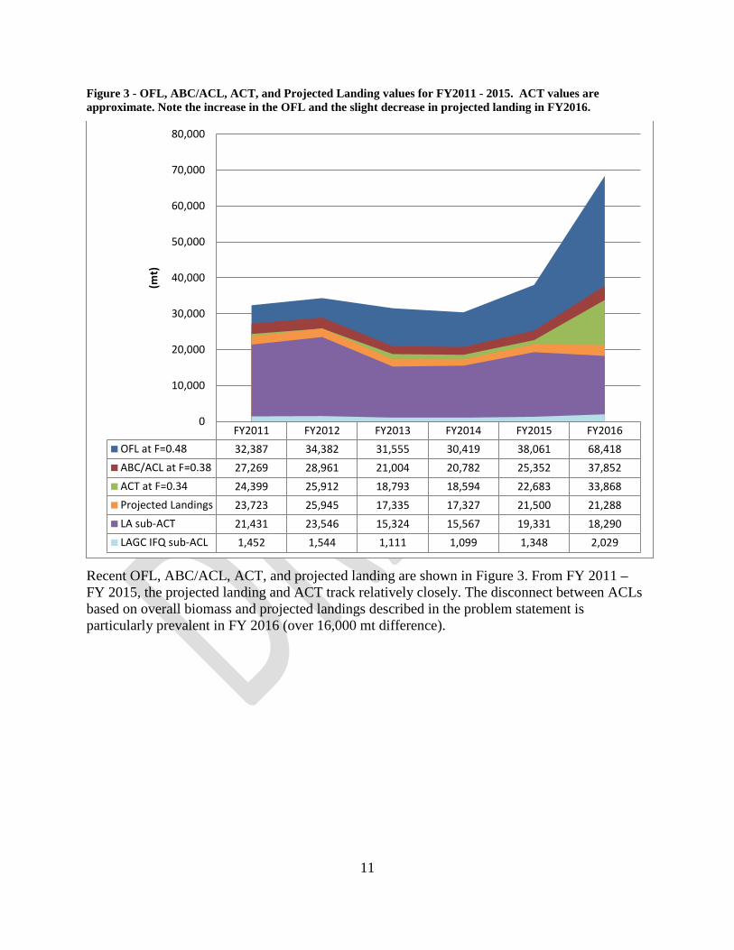
Figure 3 - OFL, ABC/ACL, ACT, and Projected Landing values for FY2011 - 2015. ACT values are approximate. Note the increase in the OFL and the slight decrease in projected landing in FY2016.

Recent OFL, ABC/ACL, ACT, and projected landing are shown in Figure 3. From FY 2011 – FY 2015, the projected landing and ACT track relatively closely. The disconnect between ACLs based on overall biomass and projected landings described in the problem statement is particularly prevalent in FY 2016 (over 16,000 mt difference).

FY2011 FY2012 FY2013 FY2014 FY2015 FY2016OFL at F=0.48 32,387 34,382 31,555 30,419 38,061 68,418ABC/ACL at F=0.38 27,269 28,961 21,004 20,782 25,352 37,852ACT at F=0.34 24,399 25,912 18,793 18,594 22,683 33,868Projected Landings 23,723 25,945 17,335 17,327 21,500 21,288LA sub-ACT 21,431 23,546 15,324 15,567 19,331 18,290LAGC IFQ sub-ACL 1,452 1,544 1,111 1,099 1,348 2,029

0

10,000

20,000

30,000

40,000

50,000

60,000

70,000

80,000

(mt)

12

Figure 4 - Performance of LAGC IFQ landings relative to quotas, FY2011- FY2015.

FY2011 FY2012 FY2013 FY2014 FY2015 FY2016LAGC actual landings 1,382 1,511 1,095 948 1,161LAGC IFQ sub-ACL/ACT 1,452 1,544 1,111 1,099 1,348 2,029LAGC Landing as % of

ACL/ACT 95% 98% 99% 86% 86%

78%

80%

82%

84%

86%

88%

90%

92%

94%

96%

98%

100%

0

500

1,000

1,500

2,000

2,500

Perc

enta

ge o

f ACL

/ACT

land

ed

(mt)

13

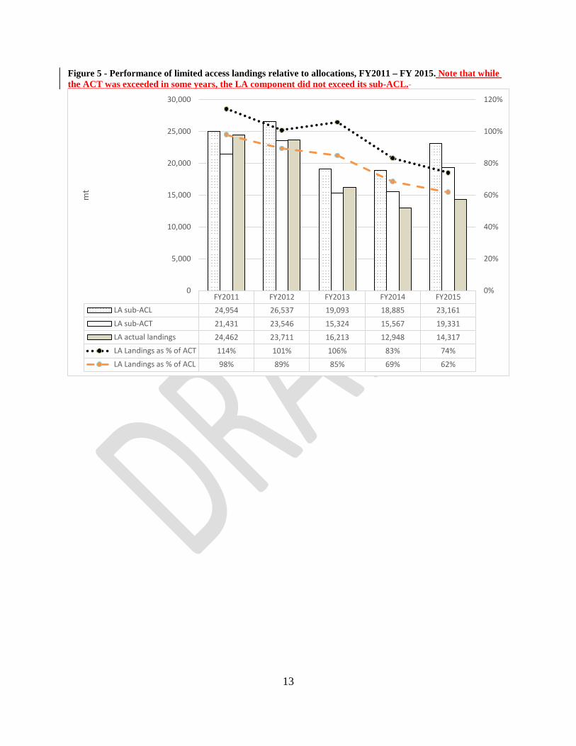
Figure 5 - Performance of limited access landings relative to allocations, FY2011 – FY 2015. Note that while the ACT was exceeded in some years, the LA component did not exceed its sub-ACL.

FY2011 FY2012 FY2013 FY2014 FY2015LA sub-ACL 24,954 26,537 19,093 18,885 23,161LA sub-ACT 21,431 23,546 15,324 15,567 19,331LA actual landings 24,462 23,711 16,213 12,948 14,317LA Landings as % of ACT 114% 101% 106% 83% 74%LA Landings as % of ACL 98% 89% 85% 69% 62%

0%

20%

40%

60%

80%

100%

120%

0

5,000

10,000

15,000

20,000

25,000

30,000

mt

14

4.0 DRAFT OBJECTIVES The annual catch limits for the LA and LAGC fisheries are consistent with decisions made in Amendment 11 (94.5% to the LA fishery and 5.5% to the LAGC fishery). However, under the current ACL structure the LA fishery allocations (DAS and allocations in access areas) are constrained by the available biomass from areas that are open, while the LAGC fishery allocation is based on available biomass from all areas. This disconnect between the catch limits and fishery allocations is more of an issue when more biomass is in closed areas and not available to the fishery. For example, in 2015 and 2016 a large proportion of total biomass was within EFH and GF closed areas as well as very large year classes of small scallops closed within scallop access areas.

As noted in the problem statement, measures adopted during and since Amendment 15 have introduced the potential for management uncertainty. Several sources of management uncertainty were identified by the PDT in A15.

An action could be developed to address these issues. The alternatives could be developed based on the draft objectives below.

1. Consider modifications to the ACL structure to set allocations that account for: a. Changes in management during and since A15 (ex: carryover). b. Spatial management.

2. Consider rReducinge potential impacts on the resource from allocations that are based on all areas, but are only fished in areas available to the fishery.

3. Consider the performance of fishery catches in both access areas and open areas (for both LA and GC IFQ components), with an emphasis on times/areas where the fishery is under performing (landings below projections).

3. Are there other measures that would address the problem statement not related to ACL structure?

15

5.0 DRAFT MEASURES

5.1 MODIFICATIONS TO SCALLOP ACL FLOWCHART

5.1.1 No Action No changes would be made to the current ACL flowchart process, described in Figure 1.

Rationale: Under the current approach established in Amendment 15, fishery catches have remained below the OFL and ABC while components of the fishery have achieved catch targets in some years.

Cons: This ACL system is not spatially explicit and does not function as well when relatively large amounts of total scallop biomass are in closed areas

5.1.2 Modify ACL Flowchart

5.1.2.1 Option A: Consider a management uncertainty buffer for the LAGC fishery A management uncertainty buffer would be specified as a percentage of LAGC IFQ sub-ACL.

Staff has identified 10% and 20% management uncertainty buffers for discussion purposes.

• Option A5% • Option A10% • Option A20%

Rationale: Measures adopted during and since Amendment 15 have introduced the potential for management uncertainty. The scallop PDT identified several sources of management uncertainty in A15, which include mortality from carry-over allowances, vessel upgrades, ability of the FMP to monitor and enforce all catch, and changes in fishing behavior that may increase landings above projected values. For example, the LAGC IFQ component is now allowed to carryover up to 15% of allocated quota from one fishing year to the next.

Cons: This modification does not address the spatial nature of the Scallop FMP. LAGC allocation would still be based on percentage of all biomass, in both open and closed areas.

16

Table 3 – Comparison of LAGC allocations when applying 5%, 10%, and 20% management uncertainty buffers and the mt difference between what the LAGC IFQ sub-ACL would have been if a management buffer were in place and actual landing. A positive value in these columns indicates that landings for the FY were less than the ACL with a management buffer applied. Values in metric tons.

FY

LAGC IFQ sub-ACL

LAGC actual landings

Option A5% Option A10% Option A20%

sub-ACL with 5% Buffer (mt)

Difference between Option A5% and Actual Landings

sub-ACL with 10% buffer (mt)

Difference between Option A10% and Actual Landings

sub-ACL with 20% buffer (mt)

Difference between Option A20% and Actual Landings

2011 1452 1382 1379 -2 1307 -75 1162 -220

2012 1544 1511 1467 -44 1390 -121 1235 -276

2013 1111 1095 1055 -40 1000 -95 889 -206

2014 1099 948 1044 96 989 41 879 -69

2015 1348 1161 1281 120 1213 52 1078 -83

2016 2029 1928 1826 1623

17

Figure 6 – Option A considers a management uncertainty buffer for the LAGC component of the fishery.

18

5.1.2.2 Option B: Consider modifying ACL structure to incorporate spatial management into catch limits based on projected landing estimates

Spatially explicit approaches would calculate ACLs/ACTs based on projected landings from areas that are open (start allocations with projected landings box at bottom of Figure 7), not to exceed a specified F ceiling (currently F=0.34 for LA, and F=0.38 for LAGC IFQ). The ceiling for either fleet could be modified; the intent is for it to reflect management uncertainty for that fleet.

There are additional approaches that the Council may consider under the umbrella of spatially explicit catch limits, such as requiring harvest of LAGC IFQ access area (AA) quota to be harvested within AAs.

Staff has identified spatially explicit management approaches for discussion purposes.

• Option B – Spatially Explicit approach

Rationale: Basing allocations only on the biomass that is available to the fishery more closely aligns allocations with the available resource; therefore is more spatially explicit. This approach may address situations when a large number of scallops are in EFH and GF closed areas, as well as very large year classes of small scallops closed within scallop access areas.

Cons: Allocations that are not spatially explicit may have a higher risk of higher fishing rates than target levels since some areas will not be open to the fishery. Table 4 - Comparison of LAGC allocations when applying a spatially explicit approach and the mt difference between what the LAGC IFQ sub-ACL would have been using a spatially explicit approach and actual landing. A negative value in indicates that landings for the FY were greater than the ACL using a spatially explicit approach. Values in metric tons.

LAGC IFQ sub-ACL

LAGC actual landings

LAGC - Option B

Difference between landings and Option B (Opt B - Landings)

FY2011 1452 1382 1257 -124 FY2012 1544 1511 1378 -132 FY2013 1111 1095 908 -186 FY2014 1099 948 907 -40 FY2015 1348 1161 1136 -25 FY2016 2029 1117

19

Table 5 - Comparison of LA allocations when applying a spatially explicit approach and the mt difference between what the LA sub-ACL would have been using a spatially explicit approach and actual landing. A negative value in indicates that landings for the FY were greater than the Option B sub-ACT “spatially explicit approach.” Values in metric tons.

LA sub-ACL

LA sub-ACT

LA actual landings

LA - Option B Difference between Option B and landings (Opt B - Landings)

FY2011 24,954 21,431 24,462 21,603 -2,859 FY2012 26,537 23,546 23,711 23,686 -25 FY2013 19,093 15,324 16,213 15,618 -595 FY2014 18,885 15,567 12,948 15,593 2,645 FY2015 23,161 19,331 14,317 19,520 5,203 FY2016 34,855 18,290 19,201

20

Figure 7 – Option B considers modifying the ACL structure to incorporate spatial management into catch limits based on projected landings estimates. There would be no changes to the process for setting the ABC/ACL and OFL.

Under Status Quo the LA sub-ACT has a ceiling of 0.34 and LAGC sub-ACT has a ceiling of 0.38, but those could be adjusted. For example, LAGC sub-ACT could be set lower than 0.38.

21

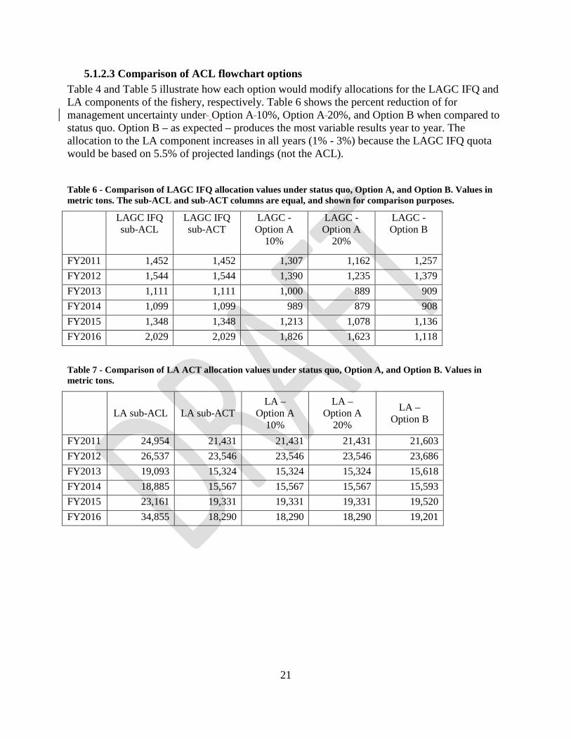
5.1.2.3 Comparison of ACL flowchart options Table 4 and Table 5 illustrate how each option would modify allocations for the LAGC IFQ and LA components of the fishery, respectively. Table 6 shows the percent reduction of for management uncertainty under Option A 10%, Option A 20%, and Option B when compared to status quo. Option B – as expected – produces the most variable results year to year. The allocation to the LA component increases in all years (1% - 3%) because the LAGC IFQ quota would be based on 5.5% of projected landings (not the ACL).

Table 6 - Comparison of LAGC IFQ allocation values under status quo, Option A, and Option B. Values in metric tons. The sub-ACL and sub-ACT columns are equal, and shown for comparison purposes.

LAGC IFQ sub-ACL

LAGC IFQ sub-ACT

LAGC - Option A

10%

LAGC - Option A

20%

LAGC - Option B

FY2011 1,452 1,452 1,307 1,162 1,257 FY2012 1,544 1,544 1,390 1,235 1,379 FY2013 1,111 1,111 1,000 889 909 FY2014 1,099 1,099 989 879 908 FY2015 1,348 1,348 1,213 1,078 1,136 FY2016 2,029 2,029 1,826 1,623 1,118 Table 7 - Comparison of LA ACT allocation values under status quo, Option A, and Option B. Values in metric tons.

LA sub-ACL LA sub-ACT

LA – Option A

10%

LA – Option A

20%

LA – Option B

FY2011 24,954 21,431 21,431 21,431 21,603 FY2012 26,537 23,546 23,546 23,546 23,686 FY2013 19,093 15,324 15,324 15,324 15,618 FY2014 18,885 15,567 15,567 15,567 15,593 FY2015 23,161 19,331 19,331 19,331 19,520 FY2016 34,855 18,290 18,290 18,290 19,201

22

Table 8 - Percent reduction from LA and LAGC IFQ sub-ACLs for management uncertainty under status quo, Option A 10%, Option A 20%, and Option B.

Status Quo Option A - 10% Option A - 20% Option B - Spatially

Explicit LA LAGC LA LAGC LA LAGC LA LAGC FY2011 -14% 0% -14% -10% -14% -20% -13% -15% FY2012 -11% 0% -11% -10% -11% -20% -11% -12% FY2013 -20% 0% -20% -10% -20% -20% -18% -22% FY2014 -18% 0% -18% -10% -18% -20% -17% -21% FY2015 -17% 0% -17% -10% -17% -20% -16% -19% FY2016 -48% 0% -48% -10% -48% -20% -45% -82%

23

5.2 OTHER POTENTIAL MEASURES

5.2.1.1 Consider modifying how the observer set-aside is removed from the ACL flowchart

By regulation, the observer set-aside is set at 1% of the ACL. As the set-aside is based on biomass in all areas, in some years this set aside is based on resources the fishery does not have access to. The risk of not harvesting the entire set-aside increases relative to the proportion of biomass in closed areas. However, the level of potential observer coverage may be higher if set-aside based on all area biomass, and not just areas available to the fishery. The PDT offers two alternative approaches for calculating the observer set-aside for consideration:

1. Calculate the observer set-aside based on the catch level associated with F=0.34 of the total biomass in all areas, which is the F value associated with the LA component’s ACT (rather than at the ABC/ACL at F=0.38). This is not a spatially explicit approach.

2. Calculate the set-asides as part of the projected landings in “Option B” before allocating to the LA and LAGC components. This is a spatially explicit approach.

24

Figure 8 - Comparison of approaches to setting the observer set-aside, including actual catch by fishing year. Note that the FY2015 bar for actual catch is hatched because data is preliminary.

Table 9 – Comparison of approaches to setting the observer set-asides, including actual catch by fishing year.

Allocated - 1% of ACL at F=0.38 (Status Quo)

Actual catch

1% of ACT at F=0.34

1% from Projected Landings in Option B

FY2011 273 104 244 231

FY2012 290 120 259 254

FY2013 210 174 188 167

FY2014 208 177 186 167

FY2015 254 220 227 209

FY2016 379 339 207

0

50

100

150

200

250

300

350

400

FY2011 FY2012 FY2013 FY2014 FY2015 FY2016

(mt)

Actual catch

Allocated - 1% of ACL atF=0.38 (Status Quo)

1% of ACT at F=0.34

1% from Projected Landings inOption B

25

Table 10 - Actual observer landings as a percentage of status quo (1% of ACL) and other potential options.

Allocated - 1% of ACL at F=0.38

(Status Quo)

1% of ACT at F=0.34

1% from Projected

Landings in Option B

FY2011 38% 43% 45% FY2012 41% 46% 47% FY2013 83% 93% 104% FY2014 85% 95% 106% FY2015 87% 97% 105%

Insert information about performance of observer set-aside to date – comparing projected and realized coverage by permit category and area

6.0 PDT DISCUSSION AND RECOMMENDATIONS The PDT reviewed an earlier version of this document on its March 9, 2016 conference call and supported forwarding it to the AP and Committee for additional discussion and input. The PDT recommended changes to the ACL flowcharts, suggested clarifications to the objectives section of the document to include recent changes in management. The PDT also identified a handful of additional analyses that would be useful to have for future discussions including a comparison of projected and realized estimates of fishing mortality, and comparison of target and realized observer coverage, etc.