Solid State lonics 18 & 19 (1986) 136-140 136 North-Holland, Amsterdam

A PACKAGE FOR IMPEDANCE/ADMITTANCE DATA ANALYSIS

Bernard A. BOUKAMP

Twente Universi ty of Technology, Department of Chemical Technology, Laboratory for Inorganic Chemistry and Materials Science, P.O.Box 217, 7500 AE Enschede, The Netherlands.

An out l ine is given of a Basic computer program which f a c i l i t a t e s the analysis of frequency dispersion data. With th is program an equivalent c i r c u i t , and s tar t ing values for the corres- ponding c i r cu i t parameters, can be extracted from the dispersion data. A c i r c u i t descript ion together with crude parameter values form an essential requirement for a subsequent NLLSF procedure. A b r ie f descr ipt ion is given of a frequency dispersion simulation program, also wr i t ten in Basic, which can be used to compare measured data with a calculated response. Both programs employ the Ci rcu i t Description Code (CDC), thus al lowing the use of a var ie ty of equivalent c i rcu i t s . The use of both programs is demonstrated with the analysis of a dispersion measurement performed on a sample of Sn-doped AgCrS 2, which is a pure ionic conductor.

1. INTRODUCTION

Impedance spectroscopy is f requent ly used in

the study of electrochemical systems I-6. One of

the advantages of this technique is that from

the immittance plots of the dispersion data good

visual information is obtained about the charac-

t e r i s t i c s of the electrochemical system. The

dispersion is general ly analyzed with the use of

an equivalent c i r c u i t as model, in which the

various c i r c u i t elements are related to the

respective processes in the system, e.g. ionic

conduct iv i ty , double layer capacitance, Warburg

d i f fus ion , e tc . . In many cases the c i r c u i t

parameters may be extracted using simple graph-

ical means. However, i f the time constants of

the respective subcircui ts are r e l a t i v e l y close

together the frequency dispersion cannot be

devided in d i s t i nc t separate regions. This is

also true i f elements with a f ract iona l power

dependence on frequency are present, e.g.

Warburg or Constant Phase Elements (CPE7-9),

because the modulus of such an element varies

sub-l inear with frequency, extending i t s

inf luence over a large frequency range in the

dispersion.

In these cases a l l c i r c u i t parameters must be

0 167-2738/86/$ 03.50 © Elsevier Science Publishers B.V. (North-Holland Physics Publishing Division)

adjusted simultaneously, in order to f i t the

equivalent c i r cu i t response to the measured dis-

persion. This can be accomplished through the

use of a special Non-Linear Least Squares F i t

(NLLSF) procedure I0-12 In order to use such a

NLLSF procedure e f f ec t i ve l y one must know the

shape of the equivalent c i r cu i t and have a set

of adequate s tar t ing values for the adjustable

c i r c u i t parameters.

This information can be obtained by a step-

wise analysis of the dispersion data in an

immittance diagram. The most prominent parts

are located f i r s t and the corresponding elements

are removed from the c i r c u i t , substracting the i r

dispersion from the overal frequency dispersion.

The use of personal computers, which have moder-

ate graphics capab i l i t i es , can be of great advantage in this analysis.

In th is paper an out l ine is given of such an

analysis program. In many cases th is program

w i l l y ie ld a sui table equivalent c i r c u i t ,

together with an adequate set of s tar t ing values

For a subsequent NLLSF procedure. The interme-

diate and f ina l f i t results may be compared with

the measured data using a dispersion simulation

program, which w i l l be discussed b r ie f l y . Both

B.A. Boukamp / A package for impedance~admittance data analysis 137

programs use the C i rcu i t Description Code 12'13

(CDC), which allows the use of a var ie ty of

equivalent c i rcu i ts with these programs without

a need for rewr i t ing the source code.

2. OUTLINE OF CIRCUIT ANALYSIS PROGRAM

Crude values for the adjustable parameters

are obtained through simple "graphical" means.

The inter face response of an ionic conductor can

often be modeled as a to ta l ionic resistance

(grain boundary + ionic resistance) in series

with a CPE element, sometimes combined with a

capacitance 14. In th is par t ia l dispersion, in

the impedance representat ion, a sui table point

is selected through which a tangential l i ne is

drawn. The intersect ion with the real axis

gives the to ta l resistance, while the f rac t iona l

exponent, n, of the CPE is found from the slope.

The dispersion re la t i on for the CPE is given by 9

Y*(w) = Yo . (j~)n (1)

The factor Yo is found from the imaginary value

of the selected data point , Z~':

Yo : -sinn-~ -~ / Z" . co n (2) 1 1

An estimate for the capacitance can be found

by substracting at the low frequency l i m i t , ~ I '

the calculated CPE response from the imaginary i I . part of the measurement, Z I .

C = I / w I (Z~' - ml n. s in-~ /Yo) (3)

A s imi lar procedure is used for the analysis

of the bulk response at the high frequency l i m i t

of the dispersion, but now in the admittance

representation. Here a resistance in para l le l

with a CPE and/or capacitance is obtained.

When there is l i t t l e interference with the

dispersion of the adjacent subci rcu i t , these

values can be used for a subsequent simple

NLLS-fit by the program, see below. Otherwise,

the parameters for the adjacent subcircui t must

be obtained in order to perform a NLLS-fit for

the combined subcircuits. To th is purpose, the

CPE (and capacitance) dispersion is removed from

the to ta l dispersion, thus exposing the disper-

sion of the adjacent subcircui t more c lear ly .

Generally the next subcircui t can be regarded

as a para l le l combination of a CPE and a resis-

tance (e.g. grain boundary immittance) in series

with another resistance. This results in a

depressed semi-circle in the immittance diagrams.

By choosing a set of three data points the

program can f i t a c i r c l e , and give values for the

resistances, as well as the CPE parameters.

The f i t t i n g of a set of subcircuits is per-

formed in the impedance representation to a

selected part of the dispersion curve. An ana-

l i t i c a l search procedure, which has been

described elsewhere 12, is used. The error func-

t ion f i t s the real and imaginary parts simul-

taneously, using one weight factor:

(Z~-Z'(w~)2+ (Z" Z"(~ ) i • i - - i -

where Z*-Z'+'Z" is the measured data set and i - i J i Z*(m) represents the calculated f i t response.

The weight factors are inversely proport ional

to the square of the modulus of the measurements:

w i = I / IZ* 2 -i i , (5)

which insures that a l l data sets contr ibute

equal ly to the error funct ion 15.

The calculat ion of the c i r c u i t response in

the f i t procedure is based on a Ci rcu i t Des-

c r ip t ion Code (CDC) 12'13, which uniquely repre-

sents the equivalent c i r cu i t . The CDC, which is

interpreted by the program, acts as a set of

pointers to a corresponding set of subroutines

which calculate the ind iv idual responses of the

d i f f e ren t types of c i r cu i t elements. The par-

t i a l der ivat ives of the error function with res-

pect to the adjustable parameters, are calcu-

lated in the same subroutines and at the same

time. This provides for a very compact source

code for the f i t procedure.

3. DISPERSION SIMULATION PROGRAM

Through the use of the CDC this program can

138 B.A. Boukamp / A package for impedance~admittance data analysis

calculate the frequency dispersion of d i f f e ren t

complex equivalent c i r c u i t s , which may include

various d i f fus ion related dispersions 13'16. The

calculated dispersion can be compared to actual

measurements in both immittance diagrams and in

a Bode p lo t .

The qua l i t y of a NLLS-fit resu l t is best seen

in a"F i t Qual i ty" p lot (FQ-plot). In th is p lo t

the re la t i ve deviat ions of the rea l , Are, and

imaginary, Aim, parts are plot ted against log(~J,

wi th: - -

Arei - i Z*i I and Aim.=1 I Z;i (6

For a good f i t these deviat ions should be d is-

t r ibu ted randomly around the frequency axis.

5

T< O

O 3 O ,~2

1 2 3 4 5 6 Z' , (*103ohm)

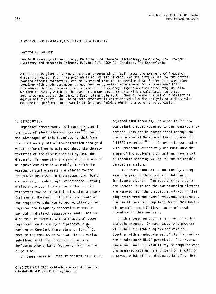
FIGURE 2 Impedance diagram showing the tangent ial l i ne for the estimation of the inter face parameters.

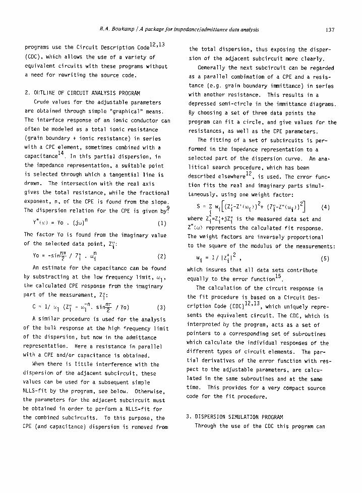
4. EXAMPLE OF DATA ANALYSIS

The use of the data analysis program is demon-

strated with a frequency dispersion measurement

of a sample of AgCrS 2 doped with 10% SnS~. This

layer compound is a pure ion ic conductor ~7. The

ac-conduct iv i ty was measured on a sample with

i o n i c a l l y blocking gold electrodes, using a

Solartron 1250 FRA. The data acquis i t ion and

correct ion was performed with an Apple I I com-

puter. The frequency range was 655 mHz to 65.5

kHz. The dispersion, measured at 298 K, is

given in the admittance p lot of f i g . i . From

T2

S

%

Ago.9CrogSno.lS2 T = 298 K

65535 Hz o

o o

oooOO o ° ° ° ° ° O o o o o °

,~o-g~T55.35imHz i i , ,

Y' ( x1 mho}

FIGURE 1 Admittance diagram of the measured dispersion.

f i r s t observation the equivalent c i r c u i t seems

quite simple, a bulk CPE in para l le l wi th the

ion ic resistance, and an inter face element

(Warburg or CPE).

As the inter face dispersion is most pronoun-

ced i t is used for the f i r s t step in the ana-

l ys i s . With a selected point the tangent ial

l i ne option (eqs 2,3) is used, resu l t ing in

crude values for the ion ic resistance and the

CPE parameters, f i g . 2. With the NLLS-fit an

optimized set is obtained. Next the response

of the inter face CPE is substracted from the

ent i re data set. The resu l t ing dispersion is

given in f i g . 3. This admittance p lo t obvious-

l y represents two in te r fe r ing subc i rcu i ts .

The parameters of the high frequency (bulk)

CPE are estimated using the tangent ial l i ne

option in the admittance representation ( f i g .

3). A subsequent NLLS-fit is not useful as the

inf luence of the medium frequency dispersion

might extend in to the high frequency d ispers ion

As an approximation the bulk CPE dispersion is

substracted from the modified data set, leaving

a depressed semi-c i rc le. A c i r c le is f i t t e d by

the program through three selected points in

th is dispersion, y ie ld ing values for the res is-

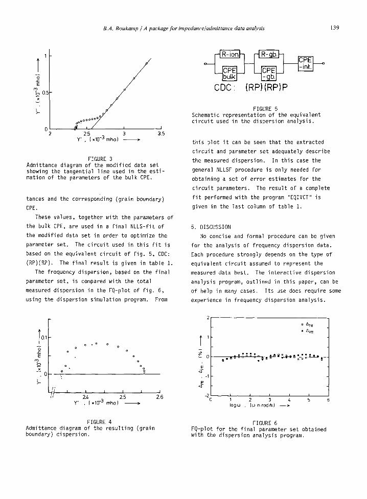
B.A. Boukamp / A package for impedance~admittance data analysis 139

1

T -S

0.5 x

0 I 2 35

ooOOOO oo°° ,

2.5 3 Y' , ( xlO -3 m h o ) >

FIGURE 3 Admittance diagram of the modified data set showing the tangential l i ne used in the es t i - mation of the parameters of the bulk CPE.

tances and the corresponding (grain boundary)

CPE.

These values, together with the parameters of

the bulk CPE, are used in a f i na l NLLS-fit of

the modified data set in order to optimize the

parameter set. The c i r c u i t used in th is f i t is

based on the equivalent c i r c u i t of f i g . 5, CDC:

(RP)(RP). The f ina l resu l t is given in table i .

The frequency dispersion, based on the f ina l

parameter set, is compared with the to ta l

measured dispersion in the FQ-plot of f i g . 6,

using the dispersion simulation program. From

T O.1

c -

E

x

0

0 0 0 0

o o

o

o

o . o

o g !

!.,

4/ J i I

I I I I

2.4 2.5 y' , { x 10 -3 mho ) ~-

I

2.6

FIGURE 4 Admittance diagram of the resul t ing (grain boundary) dispersion.

C D C (IRP) (RP)P

FIGURE 5 Schematic representation of the equivalent c i r cu i t used in the dispersion analysis.

th is p lot i t can be seen that the extracted

c i r c u i t and parameter set adequately describe

the measured dispersion. In th is case the

general NLLSF procedure is only needed for

obtaining a set of error estimates for the

c i r cu i t parameters. The resul t of a complete

f i t performed with the program "EQIVCT" is

given in the last column of table i .

5. DISCUSSION

No concise and formal procedure can be given

for the analysis of frequency dispersion data.

Each procedure strongly depends on the type of

equivalent c i r cu i t assumed to represent the

measured data best. The in terac t ive dispersion

analysis program, out l ined in th is paper, can be

of help in many cases. I ts use does require some

experience in frequency dispersion analysis.

a A re

• A im t' _ - 0 ' = ' " , ~ o .

E

. -1

I I I 1 I

-20 1 2 3 4 5 Iogca , (u in rod/s) )

FIGURE 6 FQ-plot for the f ina l parameter set obtained with the dispersion analysis program.

140 B.A. Boukamp / A package for impedance~admittance data analysis

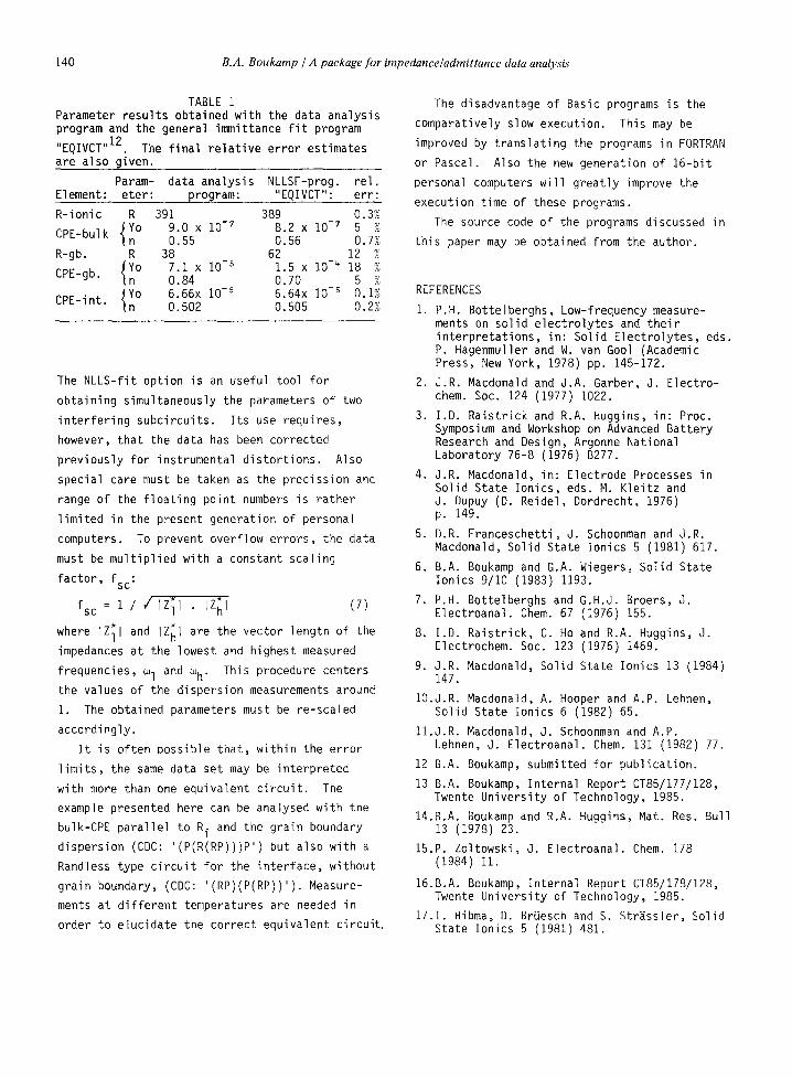
TABLE 1 Parameter resul ts obtained with the data analysis program and the general immittance f i t program

"EQIVCT ''12. The f i na l r e l a t i ve error estimates are also given.

Param- data analysis NLLSF-prog. re l . Element: eter: program: "EQIVCT": err :

R- ionic R 391 389 0.3%

CPE-bulk IYn ° 9.00.55x I0 -7 0.56 8.2 x i0 -~ 0.7%5 %

R-gb. R 38 62 12 % ~Yo 7 . 1 x 10 -s 1.5 x 10-" 18 % CPE-gb. ~n O.84 O.7O 5 % ~Yo 6.66x I0 -s 6.64x 10 -s 0.1%

CPE-int. )n 0.502 0.505 0.2%

The NLLS-fi t option is an useful tool for

obtaining simultaneously the parameters of two

i n te r fe r i ng subc i rcu i ts . I t s use requires,

however, that the data has been corrected

previously for instrumental d i s to r t i ons . Also

special care must be taken as the precission and

range of the f l oa t i ng point numbers is rather

l imi ted in the present generation of personal

computers. To prevent overflow errors, the data

must be mu l t ip l ied with a constant scal ing

fac tor , fsc:

= Z ~ fsc 1 / / IZ~l I h I (7)

where IZ~I and IZ* h I are the vector length of the

impedances at the lowest and highest measured

frequencies, ml and w h. This procedure centers

the values of the dispersion measurements around

1. The obtained parameters must be re-scaled

accordingly.

I t is often possible tha t , w i th in the error

l i m i t s , the same data set may be interpreted

with more than one equivalent c i r c u i t . The

example presented here can be analysed with the

bulk-CPE para l le l to R i and the grain boundary

dispersion (CDC: '(P(R(RP)))P') but also with a

Randless type c i r c u i t for the in ter face, wi thout

grain boundary, (CDC: '(RP)(P(RP))') . Measure-

ments at d i f f e ren t temperatures are needed in

order to elucidate the correct equivalent c i rcu i t .

The disadvantage of Basic programs is the

comparatively slow execution. This may be

improved by t rans la t ing the programs in FORTRAN

or Pascal. Also the new generation of 16-bi t

personal computers w i l l great ly improve the

execution time of these programs.

The source code of the programs discussed in

th is paper may be obtained from the author.

REFERENCES

1. P.H. Bottelberghs, Low-frequency measure- ments on sol id e lec t ro ly tes and the i r in te rp re ta t ions , in: Solid E lect ro ly tes , eds. P. Hagenmuller and W. van Gool (Academic Press, New York, 1978) pp. 145-172.

2. J.R. Macdonald and J.A, Garber, J. Electro- chem. Soc. 124 (1977) 1022.

3. I.D. Rais t r ick and R.A. Huggins, in: Proc. Symposium and Workshop on Advanced Battery Research and Design, Argonne National Laboratory 76-8 (1976) B277.

4. J.R. Macdonald, in : Electrode Processes in Solid State lon ics, eds. M. K le i tz and J. Dupuy (D. Reidel, Dordrecht, 1976) p. 149,

5. D.R. Franceschett i , J. Schoonman and J.R. Macdonald, Solid State lonics 5 (1981) 617.

6. B.A. Boukamp and G.A. Wiegers, Solid State lonics 9/10 (1983) 1193.

7. P.H. Bottelberghs and G.H.J. Broers, J. Electroanal. Chem. 67 (1976) 155.

8, I.D. Rais t r ick , C. Ho and R.A. Huggins, J. Electrochem. Soc. 123 (1976) 1469.

9. J.R. Macdonald, Solid State lonics 13 (1984) 147.

IO.J.R. Macdonald, A. Hooper and A.P. Lehnen, Solid State lonics 6 (1982) 65.

I I . J .R . Macdonald, J. Schoonman and A.P. Lehnen, J. Electroanal. Chem. 131 (1982) 77.

12 B.A. Boukamp, submitted for publ icat ion.

13 B.A. Boukamp, Internal Report CT85/177/128, Twente Univers i ty of Technology, 1985.

14.B.A. Boukamp and R.A. Huggins, Mat. Res. Bull 13 (1978) 23.

15.P. Zoltowski, d. Electroanal. Chem. 178 (1984) 11.

16.B.A. Boukamp, Internal Report CT85/178/128, Twente Univers i ty of Technology, 1985.

17.T. Hibma, D. Br~esch and S. Str~ssler , Solid State lonics 5 (1981) 481.