Embed Size (px)
Citation preview

Ulrich Thiessen Paul Gregory
Modelling the Structural Change of Transition Countries
Discussion Papers
Berlin, October 2005
brought to you by COREView metadata, citation and similar papers at core.ac.uk
provided by Research Papers in Economics

IMPRESSUM
© DIW Berlin, 2005
DIW Berlin Deutsches Institut für Wirtschaftsforschung Königin-Luise-Str. 5 14195 Berlin Tel. +49 (30) 897 89-0 Fax +49 (30) 897 89-200 www.diw.de
ISSN print edition 1433-0210 ISSN electronic edition 1619-4535
All rights reserved. Reproduction and distribution in any form, also in parts, requires the express written permission of DIW Berlin.
.

Discussion Papers 519
Ulrich Thießen * Paul Gregory ** Modelling the Structural Change of Transition Countries Berlin, October 2005 * German Institute of Economic Research, Department of International Economics,
[email protected] ** University of Houston, Houston, Texas,
Discussion Papers 519 List of contents
I
List of contents
Abstract ..................................................................................................................................... 1
1 Introduction ......................................................................................................................... 2
2 Methodology: An overview................................................................................................. 3
3 Descriptive statistics and stylized facts.............................................................................. 4
4 Empirical analysis ............................................................................................................... 5
5 Discussion of some results................................................................................................... 8 5.1 Sectoral employment share panel regressions ............................................................... 8 5.2 Evaluation of structural adjustment of individual countries ........................................ 11 5.3 Ex-post and ex-ante simulations of sector shares ........................................................ 13
6 Concluding remarks.......................................................................................................... 18
References ............................................................................................................................... 20
Appendix A: Table 1 .............................................................................................................. 22
Appendix B: Figures 1a-1b.................................................................................................... 23
Appendix C: Regression output ............................................................................................ 24
Appendix D: Figures 2a-2d.................................................................................................... 26
Appendix E: Figures 3-3d...................................................................................................... 28
Appendix F: Figures 4a-4i ..................................................................................................... 30

Discussion Papers 519 List of tables
II
List of tables
Tab. 1 Comparison of economic structures of Eastern European countries with averages of market economic groups, 1991 and 2001 (Appendix A)......................................................................................................... 22
Tab. 2 Panel regression results of Sectoral Employment Share Functions (Appendix C)......................................................................................................... 39
Tab. 3 Simulated changes of sectoral employment shares during 2001-2015 in Eastern European countries ................................................................................... 17
Tab. 4 Simulated average structure of Eastern European countries in 2015.................... 18
Appendix List of figures
Fig.1a Structural Deviation Indicator: Employment – Deviation of the structure of 8 new Eastern EU countries from certain country groups 1982-2001 .................. 23
Fig. 1b Structural Deviation Indicator: – Employment: Deviation of the structure of Bulgaria and Romania from certain country groups 1982-2001........................... 23
Fig. 2a Sectoral Employment Share of Agriculture in 54 Market Economies and Transition Countries .............................................................................................. 26
Fig. 2b Sectoral Employment Share of Manufacturing in 54 Market Economies and Transition Countries .............................................................................................. 26
Fig. 2c Sectoral Employment Share of Financial and Related Services in 54 Market Economies and Transition Countries .................................................................... 27
Fig. 2d Sectoral Employment Share of Community, Social, and Personal Services in 54 Market Economies and Transition Countries................................................... 27
Fig. 3a Adjustment path of the Employment Share of Agriculture in Eastern European new EU member countries and EU accession candidates during transition................................................................................................................ 28
Fig. 3b Adjustment path of the Employment Share of Manufacturing in Eastern European new EU member countries and EU accession candidates during transition................................................................................................................ 28
Fig. 3c Sectoral Employment Share of Financial Services, Real Estate and Related Services in Eastern European new EU member countries and EU accession candidates during transition................................................................................... 29
Fig. 3d Sectoral Employment Share of Community, Social, and Personal Services in Eastern European new EU member countries and EU accession candidates during transition .................................................................................................... 29
Fig. 4a Adjustment path of the Employment Share of Agriculture in Poland: Actuals and Forecasts 1990-2015.......................................................................... 30

Discussion Papers 519 List of tables
III
Fig. 4b Adjustment path of the Employment Share of Agriculture in Romania: Actuals and Forecasts 1990-2015.......................................................................... 30
Fig. 4c Adjustment path of the Employment Share of Manufacturing in Estonia: Actuals and Forecasts 1993-2015.......................................................................... 31
Fig. 4d Adjustment path of the Employment Share of Manufacturing in the Czech Republic: Actuals and Forecasts 1993-2015 ......................................................... 31
Fig. 4e Adjustment path of the Employment Share of Manufacturing in Poland: Actuals and Forecasts 1990-2015.......................................................................... 32
Fig. 4f Adjustment path of the Employment Share of Financial Services, Real Estate and Related Services in the Czech Republic: Actuals and Forecasts 1992-2015.............................................................................................................. 32
Fig. 4g Adjustment path of the Employment Share of Financial Services, Real Estate and Related Services in Hungary: Actuals and Forecasts 1991-2015 ........ 33
Fig. 4h Adjustment path of the Employment Share of Financial Services, Real Estate and Related Services in Slovenia: Actuals and Forecasts 1993-2015 ........ 33
Fig. 4i Adjustment path of the Employment Share of Community, Social, and Personal Services in Poland: Actuals and Forecasts 1990-2015........................... 34

1
Modelling the Structural Change of Transition Countries
Ulrich Thießen1 and Paul Gregory2
Abstract
The rapid changes in the transition economies must be evaluated in a comparative context.
This paper provides a comprehensive comparative analysis using a large panel data set of
market economies as a reference point. We wish to establish the extent and speed with which
the structures of the transition economies are converging towards other country groups ranked
according to income levels. This exercise provides an alternate measure of transition
“success” which is grounded in quantitative rather than subjective indicators. It also shows
future sectoral growth patterns under the assumption that remaining structural distortions will
continue to be removed.
JEL classification: O40, O57, P21
Keywords: Structural Change, Transition, Simulations.
1 German Institute for Economic Research, Berlin. Comments from participants at the conference of the European Economics and Finance Society in May 2005 at the University of Coimbra, Portugal, and of Holger Görg, Jürgen Bitzer, Wolfram Schrettl, and Philip Schröder are gratefully acknowledged. 2 University of Houston, Houston, Texas.

Discussion Papers 519 1 Introduction
2
1 Introduction
The planned socialist economies practiced centralized distribution of resources according to
“planners’ preferences” (Bergson, 1964). The rigidity of material balance planning (“planning
from the achieved level”), the deliberate choice of autarky, and a distinctive system of
priorities created deviations from market-like resource allocations. Consequently, the patterns
of resource allocation (as observed in the structure of GDP, consumer budgets, foreign trade,
and so on) in the Soviet Union and Eastern Europe differed significantly from those of market
economies at similar levels of development. These structural distortions contributed to the
stagnation and decline of the planned economies (Gregory and Stuart, 2001, Rosefielde, 1998,
Desai, 1987). The larger the deviations from normal patterns, the more difficult the transition.
Indeed, transition “success” varied inversely with the proximity to and duration of the Soviet
core model (Stuart and Panayotopouolos, 1999).
The pace of change in the transition economies, both structural and institutional, has been
rapid since 1991,3 but these changes must be evaluated in a comparative context. Such
comparative studies were recently completed for transition economies using a single cross
section of market economies to establish benchmarks for changes in the distribution of GDP
(Döhrn and Heilemann, 1996) and of labor (Raiser et al., 2004, and World Bank, 2004a).
These analyses used a breakdown of only four sectors and they employed either relatively few
observations or only income as the explanatory variable. This paper provides a more
comprehensive comparative analysis using a large unbalanced panel data set of market
economies, a more detailed sectoral breakdown of employment in nine sectors, and a
relatively large number of potential explanatory variables, including, for the first time in such
analyses, proxies for institutional characteristics. This approach yields ”benchmark“ equations
that define a ”normal“ relationship between per capita income and employment shares, which
differ from previous studies. Moreover, the estimations allow long-run ex-ante simulations of
the structure of each of the eight new Eastern European EU member countries (Czech
Republic, Estonia, Latvia, Lithuania, Hungary, Poland, Slovakia, and Slovenia) and of the
two EU accession candidates (Bulgaria and Romania).
The paper begins with a brief methodological overview in section 2. Section 3 summarizes
structural developments in the Eastern European countries under consideration, compares 3 On Eastern Europe see, for instance: Falceti, Lysenko, and Sanfey (2004), Fidmuc (2003), Havrylyshyn and van Rooden (2003), and the transition success indicators in the EBRD Transition reports. On Russia see, for instance, Gregory and Stuart (2001), chaps. 16-18, Schroeder (1998) and Tabata (1996).
Discussion Papers 519 2 Methodology: An overview
3
them with groups of market economies, and proposes a simple quantitative, aggregate
“indicator of structural deviation” to measure the structural adjustment progress. Section 4
presents the panel regression analysis and section 4 uses the results both to evaluate transition
progress in each of the considered Eastern European countries and to simulate their individual
future structural change. Section 5 concludes.
2 Methodology: An overview
The Soviet-era literature attempted to measure the deviations of planned socialist economies
from “normal“ economic structures, using the methodology pioneered by Chenery and his
associates (Chenery, 1960, Chenery and Taylor, 1968, Chenery and Syrquin, 1975). This
methodology used a cross section of market economies to estimate regression equations (that
used per capita income, size, and measures of trade orientation), whose parameters were used
to “predict“ the hypothetical structure of selected planned economies under the assumption
that they “behaved“ like market economies. Researchers found the estimated deviations from
“normal” structures of market economies to be substantial, such as the greater shares of heavy
industry, the low shares of services, the high shares of food, consumption, and the
underutilization of foreign trade.4 The transition economies, hence, started with initial
conditions inherited from their socialist past, which would be expected to be removed in the
course of a successful transition. One measure, therefore, of transition success would be the
extent to which it could be demonstrated, first, that the structural distortions were present at
the start of transition and, second, the extent to which they have been removed and with what
speed.
There has been remarkable development in electronic data bases since the end of the Soviet
era with large panels of data bases compiled by organizations such as the World Bank and the
International Labor Organization (ILO) readily available (World Bank, 2004b, ILO, 2004).
Moreover, the transition economies of the former Soviet Union and Eastern Europe have
adopted international national income accounting standards (SNA), and it is no longer
necessary to convert them to international standards. Accordingly, we are able to compare
structural change in transition economies with “normal“ structures estimated from large
unbalanced panel data sets.
4 Kuznets (1963), Gregory (1970), Ofer (1973), Schroeder and Edwards (1981), and more recently with limitations Döhrn and Heilemann (1996) and Raiser, Schaffer, and Schuchardt (2004).

Discussion Papers 519 3 Descriptive statistics and stylized facts
4
3 Descriptive statistics and stylized facts
The descriptive statistics of the course of transition have been amply covered in other
publications (e.g. EBRD, 2003 and 2004, World Bank, 1996, Gros and Steinherr, 2004,
Fischer and Sahay, 2000). The pace of structural change has been positively correlated with
economic reforms; it has been most rapid in the new eastern European EU member countries.
The output decline at the start of transition was generally more severe than economists had
expected, and despite structural change, the output recovery took much longer than expected.
Poland, the transition country with the lowest cumulative output decline of “only“ 14%, was
the first to recover to its pre-transition level. Also, Poland is regarded to have been a fast
reformer.5 Not surprisingly, in Table 1 (Appendix A), which compares 1991 with 2001,
Poland’s GDP structure in 2001 was the closest to the average of 12 high income European
countries. Poland together with Latvia were even more “advanced“ than the averages of the
relatively poor EU countries Greece, Ireland,6 and Portugal with lower agricultural and
manufacturing output shares and equivalent shares of services.
In general, the table shows more rapid adjustments in transition countries’ GDP than in labor
force structures. Dividing the GDP shares by the respective labor force shares yields relative
sectoral productivities, the structures of which generally became more similar. The confusing
descriptive statistics in Table 1 can be compactly summarized by “distance“ measures of
convergence, defined as: Dk = Σi (SAcci – Ski)2, where SAcci is the average share of ith sector in
the new EU member countries or accession candidates and Ski is the average share of the ith
sector in the country group k.7 The indicator Dk measures only the relative “distance” between
the transition countries and the respective country group taking into account all sectors
simultaneously.8 The smaller D becomes, the smaller is the structural difference of the new
EU member countries and accession candidates with regard to country group k. The absolute 5 By 2004 the four transition countries with highest reform grades using the EBRD (2004) transition indicators where Hungary, Estonia, Czech Republic, and Poland, in that order with minor differences. 6 In the beginning of the considered 20 year period, Ireland was relatively poor but today it is among the ten EU states with highest per capita income. 7 The deviations are squared so as to give positive and negative values the same weight. 8 Three country groups were classified, i.e. 12 high income European countries (Austria, Belgium, Denmark, Finland, France, Germany, Italy, Netherlands, Norway, Sweden, Switzerland, United Kingdom), 33 countries with income similar to the Eastern European countries (Argentina, Bolivia, Brazil, Chile, Colombia, Costa Rica, Dominican Republic, Ecuador, El Salvador, Egypt, Honduras, India, Indonesia, Iran, Jamaica, Malaysia, Mauritania, Mexico, Morocco, Nicaragua, Pakistan, Panama, Peru, Philippines, Sri Lanka, Suriname, Syria, Thailand, Trinidad and Tobago, Tunisia, Turkey, Uruguay, Venezuela), and the three formerly poorest EU countries (Greece, Ireland, and Portugal) which received relatively high net transfers from the EU as is now the case with regard to the new EU member countries. The Eastern European countries were divided into two groups, namely the eight new EU member countries and the two EU accession candidates Bulgaria and Romania.

Discussion Papers 519 4 Empirical analysis
5
values of the indicator bear no meaning but their evolution and the comparison of values for
different country groups is of interest.
Figures 1a and 1b in Appendix B provide distance measures for employment structure for the
8 new Eastern European EU member countries and the two accession candidates (Bulgaria
and Romania), respectively.9 Surprisingly, already by 1989 and 1990 the employment
structure of the eight new Eastern European EU member countries converged towards the two
reference groups, due to labor-shedding in agriculture and employment increases in some
services sectors. Since the mid 1990s the convergence process appears to have stagnated.
Figure 1b shows that Bulgaria and Romania’s transition resulted in increasing differences in
employment structure compared to EU countries and countries with similar income.10
The indicator of structural deviation is a convenient, objective summary measure of the
structural adjustment of Eastern European countries contrary to subjective measures such as
the transition indicators produced by International Organizations. It compares changes in the
“distance“ between the transition economy and group averages of reference country groups.
The approach does not use econometric analysis to “benchmark“ the transition economy
relative to some hypothetical “normal“ structure as did Chenery and his associates but its
results are very similar to those obtained from the following regression analysis.
4 Empirical analysis
We use panel regressions for a large group of economies to calculate Chenery-type
“benchmark” sector shares for transition economies. Panel regressions were run for a
maximum of 54 selected developing and developed economies to explain their sectoral
employment shares.11 For reasons of space, we report the results only of four of the total of
9 The International Labour Organization (ILO) provides employment data for a large number of countries and years and for 9 sectors: 1. Agriculture, Hunting, Forestry and Fishing, 2. Mining and Quarrying, 3. Manu-facturing, 4. Electricity, Gas and Water, 5. Construction, 6. Wholesale, Retail Trade, Restaurants, and Hotels, 7.Transport, Storage and Communication, 8. Financing, Insurance, Real Estate and Business Services, 9. Comm-unity, Social and Personal Services. 10 This is, however, due to persistent increases in already far exaggerated agricultural employment and no employment growth in financial and some other services, and it is not due to too little labour shedding in industry. 11 Only market economies were included that do not have unusual or special characteristics, such as, for instance, a very small population (less than one million) or an extremely large share of GDP derived from extraction of natural ressources. The chosen countries were: Argentina, Australia, Austria, Belgium, Bolivia, Brazil, Canada, Chile, Colombia, Costa Rica, Cyprus, Denmark, Dominican Republic, Ecuador, Egypt, El Salvador, Finland, France, Germany, Greece, Honduras, India, Indonesia, Ireland, Israel, Italy, Jamaica, Japan, Korea, Malta, Mauritania, Mexico, Morocco, Netherlands, New Zealand, Nicaragua, Norway, Pakistan, Panama, Philippines, Portugal, Puerto Rico, Spain, Sri Lanka, Sweden, Switzerland, Thailand, Trinidad and Tobago, Turkey, United Kingdom, USA, Uruguay, and Venezuela.

Discussion Papers 519 4 Empirical analysis
6
nine sectors, namely two sectors whose employment shares eventually decline as income
rises, i.e. agriculture and manufacturing, and two sectors whose employment shares increase
monotonically with income, i.e. financial services and community, social, and personal
services. These four sector shares account for an average of about 65 percent of employment
in the transition economies.
The explanatory variables included standard Chenery-type variables, i.e. per capita income
(Ypc), measured in purchasing power parities, and its square to account for non-linear
relationships, the size of the economies proxied by population (POP), the investment ratio
(Inv), and the endowment of natural resources (NR).12 We also include proxies for “openness”
(Trade), i.e. the sum of exports and imports as a ratio to GDP, human capital (HC), namely
school and higher education enrollment ratios, to measure potential effects of education, and
several variables to capture the effect of government policies (GP), i.e. the government
consumption expenditure share, tax revenues to GDP, taxes on international trade to GDP,
and military expenditure shares. We also include proxies for institutional characteristics (IC),
namely economic freedom, corruption perception, and political stability. A dummy variable
(D) is included to account for the 1997/98 Asian financial crisis in five countries (Indonesia,
Korea, Malaysia, Philippines and Thailand).13 The regressions include a constant for each
country and a time dummy for each year (cross-section and period fixed effects model).14 All
variables were transformed into natural logarithms except the dummy, the natural resource
variables, and the proxies for institutional characteristics.15
12 Agricultural resources were proxied by permenant cropland per capita. Other natural resources were proxied by a resource depletion index, defined as depletion of energy and minerals, and net forest depletion, in percent of gross national income, where each type of depletion was given equal weight. A third proxy for all natural resources was also considered, namely the share of primary exports (agricultural raw materials, ores, basic metals, and fuels) in exports of goods and services. 13 The dummy variable equals one for these two years and these five countries, and zero otherwise. 14 Formal tests of each regression strongly argued in favor of the two-way fixed effects model against the model with no fixed effects: the Hausman specification test rejected consistently the random-effects model as a valid specification and the likelihood ratio test rejected consistently the hypothesis of no fixed effects. For reasons of space the estimates for country and year dummies are, however, not reported in table 1. 15 The reasons for not transforming the institutional characteristic variables were that one of these (the index of economic freedom) had some observations that were zero, and their significance tended to be somewhat higher when not using logs. Since this was also the case regarding the natural resource variables, they were also not transformed.

Discussion Papers 519 4 Empirical analysis
7
Thus, the basic model is:
ln (LFijt/LFjt) = ai
0 + ai1 ln Ypcjt + ai
2 (ln Ypc)2jt + ai
3 ln Tradejt + ai4 ln POPjt + ai
5 ln HCjt
( +/-/? ) ( -/+/? ) ( +/-/? ) ( +/? ) ( +/? )
+ ai6 ln Invjt + ai
7 ln GPjt + ai8 NRjt + ai
9 ICjt + ai10 DAsia5, 97-98 + ui
j + vit + ei
jt (1)
( +/? ) ( ? ) ( +/? ) ( ? ) ( ? )
where i represents the sectors, j represents the countries, uj represents country specific effects,
vt represents period specific effects, and ejt is an error term.
Specific signs of the independent variables are expected only for some sectors. The expected
signs are shown in parenthesis below the variables. In most cases the signs are theoretically
indeterminate. For instance, with regard to agriculture we expect a declining labor force share
as per capita income rises (a positive sign for coefficient a1 and a negative sign for coefficient
a2), while for financial services the opposite is true. Since international trade promotes
adjustment of the production structure according to comparative advantage and thus rising
production in the long-run in all trading partner countries, a positive sign of the trade variable
is expected for sectors producing tradeable goods like agriculture and manufacturing. Country
size, measured by population, is expected to have a positive effect on sectors that produce
with economies of scale, for instance agriculture and manufacturing. Human capital is
expected to positively influence relative employment in sectors producing skill-intensive
goods and services such as manufacturing and financial services. The investment ratio may be
expected to be positively related to employment shares of sectors where production is
sensitive to investment such as manufacturing, possibly also agriculture and financial
services. No prior expectations exist as to the effects of government policies on the
employment structure. Natural resource wealth is expected to affect the employment shares of
those sectors positively, which use or process these resources. Improvements of institutions
may be expected to positively influence employment shares particularly of financial services
and manufacturing to the extent that the development of these sectors is in the long run
relatively dependent on well functioning institutions.

Discussion Papers 519 5 Discussion of some results
8
We use sectoral ILO employment data, the data for the institutional characteristics were taken
from three different sources,16 and all other data were drawn from the World Development
Indicators data base of the World Bank. The longest time period covered was 1970-2001.
Since the data on human capital were available only with relatively large data gaps, and the
institutional data begin much later, the results, with and without these variables, are not
directly comparable due to different sample periods. Given the different time periods for
various specifications, a relatively large number of regressions were performed, and selected
results are reported in Table 2 in Appendix C.
5 Discussion of some results
5.1 Sectoral employment share panel regressions
Tests for robustness of the estimated coefficient signs and statistical significance of the
explanatory variables were performed through variations of both the included independent
variables and the sample period. They confirmed that a more detailed breakdown of sectors
(more than agriculture, industry, and services) is appropriate, since specifications that
appeared to be robust differed from sector to sector. Only the income variables and
surprisingly some of the institutional variables were consistently significant and robust in all
regressions. The sensitivity of the estimations underlines potential pitfalls of panel regressions
and lead us to prefer parsimonious estimated models that include only variables whose
estimated coefficient signs and significance are robust.17 Arguably, the employment shares are
jointly determined: If the manufacturing shares increases, e.g. this will have implications for
the other shares. Thus, the equations reported in Table 2 could be jointly estimated in a
system of equations, e.g. as SURE regressions. But since our main goal was to produce ex-
post forecasts for employment shares of individual eastern European countries as accurately
as possible to use them for ex-ante forecasts, and since the specifications with the best 16 The economic freedom index was taken from the Fraser Institute (2003); the corruption perception index was taken from Transparency International (2004); the index of political stability was taken from Kaufmann et al. (2003). Missing observations for these indices were generated, if possible, though linear interpolation but the index of economic freedom starts not earlier than 1975, the corruption perception index starts not earlier than 1980, and the index of political stability starts only in 1996. Increases in these indices mean improvements, i.e. more economic freedom and political stability, and less corruption. 17 Recently, and in the context of empirical studies on FDI, Blonigen and Wang (2004) pointed to potential estimation problems when pooling data for heterogenous country groups. This is a further qualification of our results. To mitigate such potential problems we control für cross-country heterogeniety through use of dummies for each country and year. In addition, FDI studies have to use relatively poor data at the country level, which contributes to the sensitivity of results of these studies. By contrast, our study uses highly aggregated variables where measurement issues are less serious.

Discussion Papers 519 5 Discussion of some results
9
forecasting power differ from sector to sector, we performed sector specific regressions.
Despite this, the sum of the forecasted sector employment shares for each country and year
was close to 100 percent, i.e. most errors were smaller than 5 percentage points.
The results were very satisfying as shown by the high explained portion of the total variation,
the high joint significance of the independent variables in all regressions, and the generally
high significance of individual explanatory variables, except in the regressions which are
based on relatively short time periods. Also the estimated signs of the coefficients were
consistent with prior expectations.
Specifically, in the agriculture regressions for the human resource and government policy
variables were consistently insignificant, suggesting that the agricultural employment share is
not influenced by education and by the considered tax and expenditure policies. The
regressions show that agricultural employment declines as per capita income rises. Trade
affects the agricultural employment share positively, the same is true for country size (proxied
by population) and, of course, for the endowment with agricultural natural resources.
Our estimations include institutional variables, i.e. economic freedom, corruption perception,
and political stability. For agriculture they show a mixed impact since more economic
freedom promotes relative agricultural employment while higher political stability and
reductions of corruption have the opposite effect, although the sign of the corruption variable
is insignificant. This mixed result may warrant a brief discussion. One could expect that
improvements in these institutions may directly promote employment in sectors that could be
relatively sensitive to them, as, for instance, financial services and manufacturing - which was
confirmed by the regressions for these two sectors - and thereby have a negative impact on
other sectors like agriculture. On this basis, the estimated negative signs of political stability
and corruption perception in the regressions for agriculture would be plausible. That
economic freedom in these regressions has the opposite, positive sign, suggests that the three
institutional variables cannot be interpreted as meaning the same and they may not be
aggregated but rather they have individual weight and effects. Thus, economic freedom could
have a meaning similar to more liberal and intensive international trade, which has an
estimated positive sign in all regressions for agriculture, whereas the other two institutional
variables (corruption perception and political stability) could have a meaning similar to
efficient government institutions, whose improvements may result in less agricultural
employment due to rising employment in other sectors.

Discussion Papers 519 5 Discussion of some results
10
The regressions for manufacturing show that similar to agriculture its employment share
eventually declines permanently as per capita income rises. Also similar to agriculture,
international trade and the country size (measured by population) promote relative
manufacturing employment. The latter influence may underline economies of scale effects.
The endowment with natural resources has a quantitatively important negative influence,
indicating that manufacturing employment does not benefit, on average, from natural
resources. Surprisingly, the measured beneficial influence of education on manufacturing
employment is not consistently significant and the investment ratio was consistently
insignificant. All considered government policy variables (the tax and expenditure ratios)
were also almost always insignificant, indicating that governments may have no or little
influence on the structure through these policies. But the regressions suggest that
manufacturing employment is positively and significantly influenced by improvements of the
institutional variables. This has particular importance for the transition countries, because
their manufacturing employment shares even in the most advanced new Eastern EU member
states are still substantially above “normality” and thus the need for continuing reductions in
relative manufacturing employment in these countries could be dampened through continuous
improvements of these institutions.
Turning to the regressions for the two services sectors financial and related services, and
community, social, and personal services (equations 3 and 4 in Table 2, Appendix C), it was
found that very few explanatory variables have been consistently significant and had robust
estimated coefficient signs: Only per capita income and surprisingly both the education level
and the institutional variables were robust explanatory variables. The influence of per capita
income is such that both services shares would continuously rise as income grows. The
education level had a positive, consistently significant and quantitatively considerable impact
on both services shares. The consistently significant influence of the institutional variables
was positive for financial services and negative for community, social, and personal services.
That relative employment in financial services is sensitive to improvements in institutions
may appear plausible because development of this sector very much depends on reliable and
credible institutions. That relative employment in community, social, and personal services is
reduced by improvements in institutions is not immediately plausible. However, employment
in this sector is a conglomerate of private and especially government employment, where the
latter is dominating, but the data at present do not allow to split these two. To isolate relative
government employment could, however, be important, if the estimated negative effect of

Discussion Papers 519 5 Discussion of some results
11
institutional variables results, for instance, from increased efficiency and thus less relative
government employment in response to improved institutions, and given that there is no
reason to assume that such improvements would reduce relative employment in personal
services.
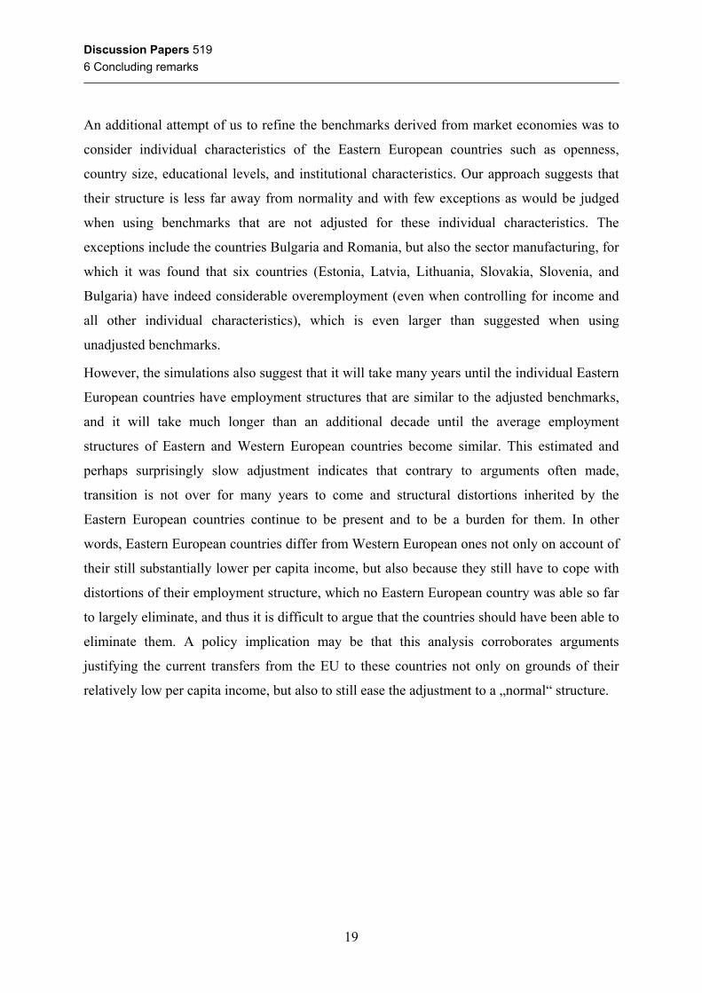
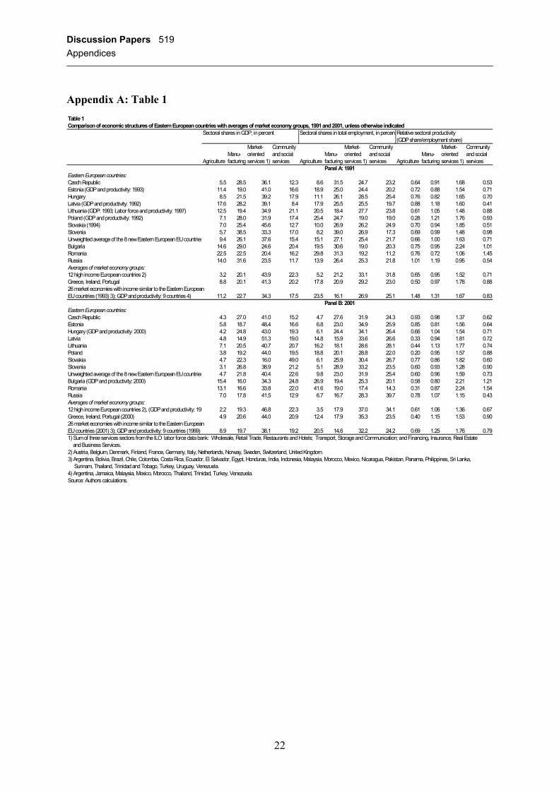
Figures 2a – 2d, Appendix D, show the estimated relationship between the four sectoral
employment shares and per capita income for the selected 54 market economies. In each
figure only two benchmark equations are plotted, namely those that define the upper and
lower limit of all estimated relationships for each sector.18 As can be seen, the consideration
of institutional variables has a small but clear impact on the estimated “normal” or
“benchmark” structure at a given level of per capita income.
The figures also show the long run average employment shares and per capita incomes of the
54 market economies, where for each country the longest available period was used. These
long run averages are also shown for the transition countries (the 8 new EU member states
and 2 accession candidates, and 16 other transition countries) but only for the period since
1990 and in some cases with only few years as dictated by data availability. The figures
suggest that with higher income the structures of the countries become increasingly similar
with few outliers. We also see that employment in agriculture, financial services, and
community, social, and personal services has in most EU accession countries (represented by
triangles) already come close to “normality” (Figures 2a, 2c, and 2d) but the average
manufacturing employment shares in several of these countries have still been considerably
away from the benchmarks (Figure 2b).
5.2 Evaluation of structural adjustment of individual countries
The benchmark regressions are used to evaluate the adjustment process of the sectoral
employment shares for each of the eight new EU member countries and the two EU accession
candidates.19 Figures 3a – 3d, Appendix E, show these individual adjustment paths, where for
each country as many years as available during transition were plotted. Each point on the 18 In order to derive the plotted curves from the panel regression output we used an average of the estimated cross-section fixed effects and an average of each considered explanatory variables over all included countries and years. The estimated period fixed effects were omitted. 19 Only two benchmark equations are plotted, namely those that define the upper and lower limit of all estimated relationships for each sector. In order to derive the benchmark curves from the panel regression output we used an average of the estimated cross-section fixed effects and an average of each considered explanatory variable over all included countries and years. The estimated period fixed effects were omitted.
Discussion Papers 519 5 Discussion of some results
12
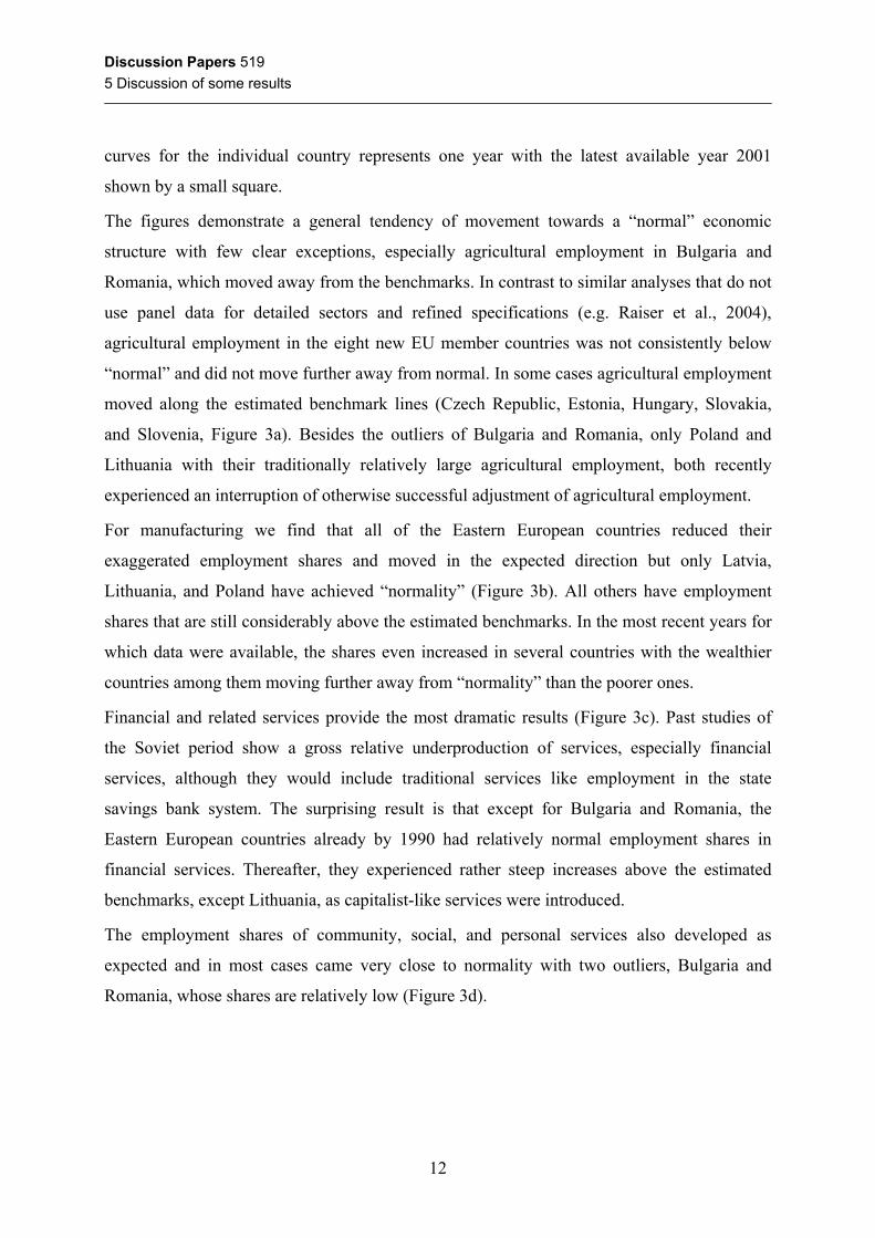
curves for the individual country represents one year with the latest available year 2001
shown by a small square.
The figures demonstrate a general tendency of movement towards a “normal” economic
structure with few clear exceptions, especially agricultural employment in Bulgaria and
Romania, which moved away from the benchmarks. In contrast to similar analyses that do not
use panel data for detailed sectors and refined specifications (e.g. Raiser et al., 2004),
agricultural employment in the eight new EU member countries was not consistently below
“normal” and did not move further away from normal. In some cases agricultural employment
moved along the estimated benchmark lines (Czech Republic, Estonia, Hungary, Slovakia,
and Slovenia, Figure 3a). Besides the outliers of Bulgaria and Romania, only Poland and
Lithuania with their traditionally relatively large agricultural employment, both recently
experienced an interruption of otherwise successful adjustment of agricultural employment.
For manufacturing we find that all of the Eastern European countries reduced their
exaggerated employment shares and moved in the expected direction but only Latvia,
Lithuania, and Poland have achieved “normality” (Figure 3b). All others have employment
shares that are still considerably above the estimated benchmarks. In the most recent years for
which data were available, the shares even increased in several countries with the wealthier
countries among them moving further away from “normality” than the poorer ones.
Financial and related services provide the most dramatic results (Figure 3c). Past studies of
the Soviet period show a gross relative underproduction of services, especially financial
services, although they would include traditional services like employment in the state
savings bank system. The surprising result is that except for Bulgaria and Romania, the
Eastern European countries already by 1990 had relatively normal employment shares in
financial services. Thereafter, they experienced rather steep increases above the estimated
benchmarks, except Lithuania, as capitalist-like services were introduced.
The employment shares of community, social, and personal services also developed as
expected and in most cases came very close to normality with two outliers, Bulgaria and
Romania, whose shares are relatively low (Figure 3d).
Discussion Papers 519 5 Discussion of some results
13
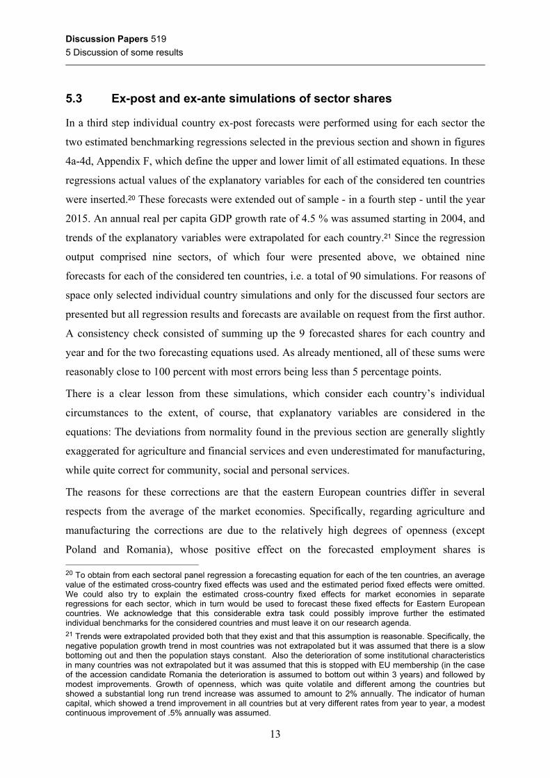
5.3 Ex-post and ex-ante simulations of sector shares
In a third step individual country ex-post forecasts were performed using for each sector the
two estimated benchmarking regressions selected in the previous section and shown in figures
4a-4d, Appendix F, which define the upper and lower limit of all estimated equations. In these
regressions actual values of the explanatory variables for each of the considered ten countries
were inserted.20 These forecasts were extended out of sample - in a fourth step - until the year
2015. An annual real per capita GDP growth rate of 4.5 % was assumed starting in 2004, and
trends of the explanatory variables were extrapolated for each country.21 Since the regression
output comprised nine sectors, of which four were presented above, we obtained nine
forecasts for each of the considered ten countries, i.e. a total of 90 simulations. For reasons of
space only selected individual country simulations and only for the discussed four sectors are
presented but all regression results and forecasts are available on request from the first author.
A consistency check consisted of summing up the 9 forecasted shares for each country and
year and for the two forecasting equations used. As already mentioned, all of these sums were
reasonably close to 100 percent with most errors being less than 5 percentage points.
There is a clear lesson from these simulations, which consider each country’s individual
circumstances to the extent, of course, that explanatory variables are considered in the
equations: The deviations from normality found in the previous section are generally slightly
exaggerated for agriculture and financial services and even underestimated for manufacturing,
while quite correct for community, social and personal services.
The reasons for these corrections are that the eastern European countries differ in several
respects from the average of the market economies. Specifically, regarding agriculture and
manufacturing the corrections are due to the relatively high degrees of openness (except
Poland and Romania), whose positive effect on the forecasted employment shares is 20 To obtain from each sectoral panel regression a forecasting equation for each of the ten countries, an average value of the estimated cross-country fixed effects was used and the estimated period fixed effects were omitted. We could also try to explain the estimated cross-country fixed effects for market economies in separate regressions for each sector, which in turn would be used to forecast these fixed effects for Eastern European countries. We acknowledge that this considerable extra task could possibly improve further the estimated individual benchmarks for the considered countries and must leave it on our research agenda. 21 Trends were extrapolated provided both that they exist and that this assumption is reasonable. Specifically, the negative population growth trend in most countries was not extrapolated but it was assumed that there is a slow bottoming out and then the population stays constant. Also the deterioration of some institutional characteristics in many countries was not extrapolated but it was assumed that this is stopped with EU membership (in the case of the accession candidate Romania the deterioration is assumed to bottom out within 3 years) and followed by modest improvements. Growth of openness, which was quite volatile and different among the countries but showed a substantial long run trend increase was assumed to amount to 2% annually. The indicator of human capital, which showed a trend improvement in all countries but at very different rates from year to year, a modest continuous improvement of .5% annually was assumed.

Discussion Papers 519 5 Discussion of some results
14
somewhat dampened by the relatively small country sizes measured by population (except
Poland and Romania). In the regressions for financial services these variables were not
included, so that the corrections for this sector are due to generally somewhat higher
educational levels and somewhat lower levels of the institutional characteristics (except the
political stability indicator) of the Eastern European countries relative to the average of
market economies. This resulted in relatively broad corridors of the individual sector forecasts
for the ten Eastern European countries.
Thus, regarding agriculture, the actual past employment shares of most Eastern European
countries have either been within the corridor of the two ex-post forecasts or rather close to it.
The only outliers with very substantial overemployment were Latvia, Lithuania, and, of
course, Bulgaria and Romania, but not, as is often argued, Poland. As an example, Figure 4a,
Appendix F, shows for Poland, that the individualized forecast shows less overemployment
than when using the unadjusted benchmark lines of Figure 3a, Appendix E. Figure 4a,
Appendix F, and the following ones incorporate the ex-ante forecasts. For all ex-ante
simulations the real per capita income growth assumption was 4.5% annually until the end of
the forecast horizon 2015. Each point on the curves in the graphs represents one year. The
midpoint of the forecasted corridor in 2015 may be interpreted as the most likely respective
sector share in that year. In addition to the other assumptions this implicitly assumes that all
remaining distortions from the former planned economy period would be eliminated by 2015
so that by then there is no systemic difference any more between the ten Eastern European
countries and the group of 54 market economies. Also, an implicit assumption is that there are
no bottlenecks in labor qualifications or other reasons, which cause frictions of labor
movements from shrinking to growing sectors.
A dotted line indicates the potential evolution of sector shares and connects the last available
actual combination of sector share and per capita income in 2001 with the midpoint of the
forecasts for 2015.
As an example for the four countries whose agricultural employment was even above the
individualized forecasts (Latvia, Lithuania, Bulgaria, Romania), Figure 4b, Appendix F,
shows for Romania relatively high ex-post simulated “normal” employment shares of about
13-15% for the first decade of transition, which decline very slowly during the future. This is
3 percentage points higher than when using the unadjusted benchmark regressions.

Discussion Papers 519 5 Discussion of some results
15
Manufacturing is the sector where the individualized forecasts yield the largest corrections of
the unadjusted benchmark lines. These simulations suggest that the latter are underestimating
the deviations from normality for the countries Estonia, Latvia, Lithuania, Slovakia, Slovenia,
and Bulgaria. For the other countries (Czech Republic, Hungary, Poland and Romania) the
individualized ex-post simulations largely confirm the overemployment suggested by the
unadjusted benchmark lines.
As examples for the two groups, Figures 4c and 4d, Appendix F, respectively, show the
results for Estonia, it belongs to the first group, and the Czech Republic, which belongs to the
second group.
Also shown are forecasts for Poland (Figure 4e, Appendix F), because Poland is the only
country of all ten, where the simulations suggest no further decline in relative manufacturing
employment but rather continuous moderate increases. This is due to Poland’s already
relatively low employment share and its relatively large population. The latter should have a
beneficial impact on the competitiveness of manufacturing through better exploitation of
economies of scale than smaller countries may achieve.
The individualized simulations for financial services suggest that all countries, except
Lithuania, Bulgaria, and Romania, had employment shares that developed within or very
close to the forecast corridor and not, as was suggested by the unadjusted benchmark
regressions (shown in Figure 3c), substantially above it. The reasons for this are that financial
services employment is significantly and positively influenced by educational levels and by
the quality of institutions, so that the generally relatively high educational levels in the
Eastern European countries compared to the average of market economies, and their past
somewhat lower institutional qualities (except political stability) resulted in relatively broad
forecast corridors. As examples, Figures 4f-4h, Appendix F, respectively, show the
simulations for the Czech Republic, Hungary, and Slovenia. Slovenia has already the largest
financial services sector of the ten countries which is projected to continue to grow strongly,
as all others too.
For the large sector community, social, and personal services the individualized ex-post
simulations of normal employment shares do not deviate much from the unadjusted
benchmark regressions. The ex-ante simulations show substantial relative employment growth
in this sector. As an example, Poland is shown (Figure 4i).

Discussion Papers 519 5 Discussion of some results
16
Although the simulations consider individual characteristics of each of the ten Eastern
European countries, the forecasted shifts in labor are very similar in all of these countries
(with the mentioned exception of slightly increasing Polish manufacturing employment).
In sum, these simulations show to what extent labor will shift from:
- agriculture,
- manufacturing (Poland is the only exception),
- mining and quarrying,
- electricity, gas and water, and
- transport, storage, and communication,
to the following sectors:
- some increases in construction,22
- wholesale and retail trade, restaurants and hotels,
- financial services, real estate, and related services,
- community, social, and personal services (which includes government).
Table 3 provides the average of the simulated sectoral shifts during 2001 to 2015 for the eight
new Eastern European EU member countries and all ten considered Eastern Europan
countries. As sector shares in 2015, the midpoint of the two forecasts for each sector and
country was used.
22 Eastern European countries have relatively high investment shares, which are estimated in “normal” market economies to significantly and positively influence the construction employment share, and investment ratios are assumed to remain at their relatively high levels in all Eastern European countries. Therefore, in the simulations relative employment in construction is growing in all countries.

Discussion Papers 519 5 Discussion of some results
17
Table 3 Simulated changes of sectoral employment shares during 2001-2015 in Eastern European countries (Average changes in percentage points) Sector EEU 8 1/ EEU 10 2/ Declining sectors:
Agriculture -5.4 -9.5 Mining and quarrying -0.6 -0.7 Manufacturing 3/ -4.1 -3.3 Electricity, gas and water -1.1 -1.1 Transport, storage, and communication -1.8 -1.4
Growing sectors: Construction 1.7 2.0 Wholesail and retail trade, restaurants and hotels 1.2 2.2 Financial services, real estate, and related services 4.5 4.8 Community, social, and personal services (including government) 3.9 5.0
Sum of all changes or forecast error -1.7 -2.0
1/ Czech Republic, Estonia, Hungary, Latvia, Lithuania, Poland, Slovakia, Slovenia. 2/ EU 8 + Bulgaria and Romania. 3/ With the exception of Poland whose manufacturing employment share is expected to grow moderately up to
the forecast horizon as explained in the text. Source: Own calculations.
Table 4 shows the simulated average employment structure of the considered eight and ten
Eastern European countries in 2015 and compares it with the average employment structure in
2001 of the former 15 EU member countries prior to the EU Eastern European enlargement.
The table shows that only by 2015 the average structure of the Eastern European countries
would be very similar to the current structure of the former EU 15 countries. However, since
in 2015 the structure of the former EU 15 countries will have changed with further declines of
relative employment in agriculture and manufacturing, and increases in relative employment
of services, it will take many more years for Eastern European countries to become
structurally similar to Western Europe.

Discussion Papers 519 6 Concluding remarks
18
Table 4 Simulated average structure of Eastern European countries in 2015 1/ (Average sectoral employment shares in percent) Sector EEU 8 /2 EEU 10 /3 Memorandum item:
EU 15 in 2001 4/
Agriculture 4.40 4.90 5.10 Mining and quarrying 0.21 0.25 0.25 Manufacturing 18.80 18.80 17.80 Electricity, gas and water 0.81 0.82 0.70 Transport, storage, and communication 6.13 6.21 6.60 Construction 8.80 8.50 7.80 Wholesail and retail trade, restaurants and hotels 18.20 18.30 18.70 Financial services, real estate, and related services 11.60 10.90 12.40 Community, social, and personal services (including government) 29.30 28.70 30.60 Sum of all changes or forecast error 98.30 97.40 99.90
1/ Underlying this average structure are simulated employment shares in 2015 for each country which were the midpoint of two forecasting equations as explained in the text.
2/ Czech Republic, Estonia, Hungary, Latvia, Lithuania, Poland, Slovakia, Slovenia. 3/ EU 8 + Bulgaria and Romania. 4/ 15 EU member countries prior to the EU Eastern European enlargement. Source: Own calculations.
6 Concluding remarks
The analysis suggests that the use of regressions to define benchmark equations of a „normal“
relationship between per capita income and sectoral employment shares is tricky and subject
to pitfalls that may lead to false conclusions especially when the benchmarks are used to
evaluate structural progress in transition economies and to judge which sector has
overemployment and which has underemployment. Our estimates are merely a first attempt to
use as much data as are available, including institutional country characteristics, and suggest
that only few and different explanatory variables for each sector are robust for market
economies. The period for which our institutional variables are available is relatively short
and thus the estimates which include them cannot satisfy demands for only long run empirical
analysis over several decades. Accepting this qualification, the institutional variables
appeared to be of significance in tests using the data we have: Better institutions appear to
promote growth of financial services and manufacturing at the cost of agriculture and
community, social, and personal services (including government).
Discussion Papers 519 6 Concluding remarks
19
An additional attempt of us to refine the benchmarks derived from market economies was to
consider individual characteristics of the Eastern European countries such as openness,
country size, educational levels, and institutional characteristics. Our approach suggests that
their structure is less far away from normality and with few exceptions as would be judged
when using benchmarks that are not adjusted for these individual characteristics. The
exceptions include the countries Bulgaria and Romania, but also the sector manufacturing, for
which it was found that six countries (Estonia, Latvia, Lithuania, Slovakia, Slovenia, and
Bulgaria) have indeed considerable overemployment (even when controlling for income and
all other individual characteristics), which is even larger than suggested when using
unadjusted benchmarks.
However, the simulations also suggest that it will take many years until the individual Eastern
European countries have employment structures that are similar to the adjusted benchmarks,
and it will take much longer than an additional decade until the average employment
structures of Eastern and Western European countries become similar. This estimated and
perhaps surprisingly slow adjustment indicates that contrary to arguments often made,
transition is not over for many years to come and structural distortions inherited by the
Eastern European countries continue to be present and to be a burden for them. In other
words, Eastern European countries differ from Western European ones not only on account of
their still substantially lower per capita income, but also because they still have to cope with
distortions of their employment structure, which no Eastern European country was able so far
to largely eliminate, and thus it is difficult to argue that the countries should have been able to
eliminate them. A policy implication may be that this analysis corroborates arguments
justifying the current transfers from the EU to these countries not only on grounds of their
relatively low per capita income, but also to still ease the adjustment to a „normal“ structure.

Discussion Papers 519 References
20
References
Bergson, A. (1964), “The Economics of Soviet Planning”, Yale University Press. Blonigen and Wang (2004), “Inappropriate Pooling of Wealthy and Poor Countries in Empirical FDI
Studies,” NBER Working Paper 10378, Cambridge Mass., March. Campos, N., and F. Coricelli (2002), “Growth in transition: what we know, what we don’t, and what
we should,” Journal of Economic Literature, Vol. 40 (3), pp. 793-836. Chenery, H.B. (1960), “Patterns of Industrial Growth,” American Economic Review, 50 (4), pp. 624-
654. Chenery, H.B. and L. Taylor (1968), “Development Patterns: Among Countries and Over Time”, The
Review of Economics and Statistics, 50, pp. 391-416. Chenery, H.B. and M. Syrquin (1975), “Patterns of Development”, 1950-1979. Oxford University
Press, London. P. Desai (1987), “The Soviet Economy: Problems and Prospects”, Blackwell. Döhrn, R., and U. Heilemann, (1996), “The Chenery hypothesis and structural change in Eastern
Europe”, Economics of Transition, 4 (2), pp. 411-425. European Bank for Reconstruction and Development EBRD (2003), Transition report 2003, London. European Bank for Reconstruction and Development EBRD (2004), Transition report 2004, London. Falceti, E., T. Lysenko, and P. Sanfey (2004), “Reforms and growth in transition: re-examining the
evidence”, EBRD mimeo. Fidmuc, J. (2003), “Economic Reform, democracy and growth during post-communist transition”,
European Journal of Political Economy, Vol. 19, pp. 583-604. Fischer, S., and R. Sahay (2000), “The Transition Economies after Ten Years”, Working Paper 00/30,
International Monetary Fund, Washington, DC. The Fraser Institute (2003), Annual Report 2003. Vancouver. Data retrieved from
www.freetheworld.com Gregory, P. and R. Stuart (2001), Russian and Soviet Economic Performance and Structure, 7th
edition, Addison Wesley. Gregory, P. (1970), Socialist and NonSocialist Industrialization Patterns, New York: Praeger. Gros, D., and A. Steinherr (2004), “Economic transition in central and eastern Europe: Planting the
seeds”, Cambridge University Press, Cambridge U.K. Havrylyshyn, O. and R. van Rooden (2003), “Institutions matter in transition but so do policies”,
Comparative Economic Studies, Vol. 45, pp. 2-24. International Labour Organization (ILO, 2004), ILO Bureau of Statistics, LABORSTA Internet,
www.laborsta.ilo.org. International Monetary Fund (2004), International Financial Statistics, Washington, D.C. Kaufmann, D., A. Kraay and M. Mastruzzi (2003), “Governance Matters III: Governance Indicators
for 1996-2002”, World Bank Policy Research Department Working Paper 3106, Washington. D.C., data retrieved from: www.worldbank.org/wbi/governance/pubs/ govmatters3.
Kuznets, S. (1963). “A Comparative Appraisal”, in A. Bergson and S. Kuznets (eds.), Economic Trends in the Soviet Union, Cambridge, MA: Harvard University Press.
Ofer, G. (1973), “The Service Sector in Soviet Economic Growth”, Cambridge, MA: Harvard University Press.
Raiser, M., M. E. Schaffer and J. Schuchardt (2004), “Benchmarking structural change in transition”, Structural Change and Economic Dynamics, 15, pp. 47-81.
Rosefielde, S. (ed.) (1998), “Efficiency and Russia’s Economic Recovery Potential”, Ashgate.

Discussion Papers 519 References
21
Schroeder, G. (1998), “Dimensions of Russia’s Industrial Transformation, 1992-1998: An Overview,” Post-Soviet Geography and Economics, 39 (5), pp. 243-271.
Schroeder, G. and I. Edwards (1981), “Consumption in the USSR: An International Comparison”, Joint Economic Committee, U.S. Government Printing Office, Washington, D.C.
Stuart, R. and C. Panayotopouolos (1999), “Decline and Recovery in Transition Economies: The Impact of Initial Conditions,” Post-Soviet Geography and Economics, 40 (4), pp.
Tabata, S. (1996), “Changes in the Structure and Distribution of Russian GDP in the 1990s,” Post-Soviet Geography and Economics, 37 (3), pp. 129-144.
Transparency International (2004), Corruption Perception Index, data retrieved from www.Transparency.org/cpi.
World Bank (2004a), From Transition to Development, Washington D.C., April. World Bank (2004b), World Development Indicators. Washington D.C. World Bank (1996), “From Plan to Market: World Development Report” 1996, Oxford University
Press, Oxford. World Bank and State Statistics Committee of the Government of the Russian Federation (1995),
Russian Federation: Report on the National Accounts, Washington, D.C. International Monetary Fund (2004), International Financial Statistics, Washington, D.C.
Discussion Papers 519 Appendices
22
Appendix A: Table 1 Table 1Comparison of economic structures of Eastern European countries with averages of market economy groups, 1991 and 2001, unless otherwise indicated
Sectoral shares in GDP, in percent Sectoral shares in total employment, in percentRelative sectoral productivity (GDP share/employment share)
Market- Community Market- Community Market- CommunityManu- oriented and social Manu- oriented and social Manu- oriented and social
Agriculture facturing services 1) services Agriculture facturing services 1) services Agriculture facturing services 1) servicesPanel A: 1991
Eastern European countries:Czech Republic 5.5 28.5 36.1 12.3 8.6 31.5 24.7 23.2 0.64 0.91 1.68 0.53Estonia (GDP and productivity: 1993) 11.4 19.0 41.0 16.6 18.9 25.0 24.4 20.2 0.72 0.88 1.54 0.71Hungary 8.5 21.5 39.2 17.9 11.1 26.1 28.5 25.4 0.76 0.82 1.65 0.70Latvia (GDP and productivity: 1992) 17.6 28.2 39.1 8.4 17.9 25.5 25.5 19.7 0.88 1.18 1.60 0.41Lithuania (GDP: 1993; Labor force and productivity: 1997) 12.5 19.4 34.9 21.1 20.5 18.4 27.7 23.8 0.61 1.05 1.48 0.88Poland (GDP and productivity: 1992) 7.1 28.0 31.9 17.4 25.4 24.7 19.0 19.0 0.28 1.21 1.76 0.93Slovakia (1994) 7.0 25.4 45.6 12.7 10.0 26.9 26.2 24.9 0.70 0.94 1.85 0.51Slovenia 5.7 38.5 33.3 17.0 8.2 39.0 26.9 17.3 0.69 0.99 1.48 0.98Unweighted average of the 8 new Eastern European EU countries 9.4 26.1 37.6 15.4 15.1 27.1 25.4 21.7 0.66 1.00 1.63 0.71Bulgaria 14.6 29.0 24.6 20.4 19.5 30.6 19.0 20.3 0.75 0.95 2.24 1.01Romania 22.5 22.5 20.4 16.2 29.8 31.3 19.2 11.2 0.76 0.72 1.06 1.45Russia 14.0 31.6 23.5 11.7 13.9 26.4 25.3 21.8 1.01 1.19 0.95 0.54Averages of market economy groups:12 high income European countries 2) 3.2 20.1 43.9 22.3 5.2 21.2 33.1 31.8 0.65 0.95 1.52 0.71Greece, Ireland, Portugal 8.8 20.1 41.3 20.2 17.8 20.9 29.2 23.0 0.50 0.97 1.78 0.8826 market economies with income similar to the Eastern European EU countries (1993) 3); GDP and productivity: 9 countries 4) 11.2 22.7 34.3 17.5 23.5 16.1 26.9 25.1 1.48 1.31 1.67 0.83
Panel B: 2001Eastern European countries:Czech Republic 4.3 27.0 41.0 15.2 4.7 27.6 31.9 24.3 0.93 0.98 1.37 0.62Estonia 5.8 18.7 48.4 16.6 6.8 23.0 34.9 25.9 0.85 0.81 1.56 0.64Hungary (GDP and productivity: 2000) 4.2 24.8 43.0 19.3 6.1 24.4 34.1 26.4 0.66 1.04 1.54 0.71Latvia 4.8 14.9 51.3 19.0 14.8 15.9 33.6 26.6 0.33 0.94 1.81 0.72Lithuania 7.1 20.5 40.7 20.7 16.2 18.1 28.6 28.1 0.44 1.13 1.77 0.74Poland 3.8 19.2 44.0 19.5 18.8 20.1 28.8 22.0 0.20 0.95 1.57 0.88Slovakia 4.7 22.3 16.0 49.0 6.1 25.9 30.4 26.7 0.77 0.86 1.82 0.60Slovenia 3.1 26.8 38.9 21.2 5.1 28.9 33.2 23.5 0.60 0.93 1.28 0.90Unweighted average of the 8 new Eastern European EU countries 4.7 21.8 40.4 22.6 9.8 23.0 31.9 25.4 0.60 0.96 1.59 0.73Bulgaria (GDP and productivity: 2000) 15.4 16.0 34.3 24.8 26.9 19.4 25.3 20.1 0.58 0.80 2.21 1.21Romania 13.1 16.6 33.8 22.0 41.6 19.0 17.4 14.3 0.31 0.87 2.24 1.54Russia 7.0 17.8 41.5 12.9 6.7 16.7 28.3 39.7 0.78 1.07 1.15 0.43Averages of market economy groups:12 high income European countries 2), (GDP and productivity: 199 2.2 19.3 46.8 22.3 3.5 17.9 37.0 34.1 0.61 1.06 1.36 0.67Greece, Ireland, Portugal (2000) 4.9 20.6 44.0 20.9 12.4 17.9 35.3 23.5 0.40 1.15 1.53 0.9026 market economies with income similar to the Eastern European EU countries (2001) 3); GDP and productivity: 9 countries (1999) 4 8.9 19.7 38.1 19.2 20.5 14.6 32.2 24.2 0.69 1.25 1.76 0.791) Sum of three services sectors from the ILO labor force data bank: Wholesale, Retail Trade, Restaurants and Hotels; Transport, Storage and Communication; and Financing, Insurance, Real Estate and Business Services.2) Austria, Belgium, Denmark, Finland, France, Germany, Italy, Netherlands, Norway, Sweden, Switzerland, United Kingdom.3) Argentina, Bolivia, Brazil, Chile, Colombia, Costa Rica, Ecuador, El Salvador, Egypt, Honduras, India, Indonesia, Malaysia, Morocco, Mexico, Nicaragua, Pakistan, Panama, Philippines, Sri Lanka, Surinam, Thailand, Trinidad and Tobago, Turkey, Uruguay, Venezuela.4) Argentina, Jamaica, Malaysia, Mexico, Morocco, Thailand, Trinidad, Turkey, Venezuela.Source: Authors calculations.

Discussion Papers 519 Appendices
23
Appendix B: Figures 1a – 1b
Figure 1aStructural Deviation Indicator: Employment
Deviations of the structure of 8 new eastern EU countries from certain country groups 1982-2001
0.00
0.02
0.04
0.06
0.08
0.10
0.12
0.14
1982 1983 1984 1985 1986 1987 1988 1989 1990 1991 1992 1993 1994 1995 1996 1997 1998 1999 2000 2001
8 new eastern EU countries vs. 12 high income European countries
8 new eastern EU countries vs. Greece, Ireland, and Portugal
8 new eastern EU countries vs. 33 market economies with similar income
Source: Own calculations.
Note: The index is defined as the sum of the squared deviations of 9 sectoral employment shares, which are average shares in the given 8 EU accession countries, from the respective average employment shares in other country groups.
Figure 1bStructural Deviation Indicator: Employment
Deviations of the structure of Bulgaria and Romania from certain country groups 1982-2001
0.00
0.02
0.04
0.06
0.08
0.10
0.12
0.14
0.16
1982 1983 1984 1985 1986 1987 1988 1989 1990 1991 1992 1993 1994 1995 1996 1997 1998 1999 2000 2001
Source: Own calculations.
Note: The index is defined as the sum of the squared deviations of 9 sectoral employment shares, which are average shares in given transition countries, from the respective average employment shares in other country groups.
Bulgaria, Romania vs. Greece, Ireland, Portugal
Bulgaria, Romania vs. 12 High Income European countries
Bulgaria, Romania vs. 33 market economies with similar income

Discussion Papers 519 Appendices
24
Appendix C: Regression output Table 2Panel Regression Results of Sectoral Employment Share FunctionsEquation: (1a) (1b) (1c) (1d) (1e) (2a) (2b) (2c) (2d) (2e)
Dependent Variable: Natural Logarithm of the Share of Employment in:Independent Variables:Sample period 1975-2001 1975-2001 1975-2001 1980-2001 1996-2001 1975-2001 1990-2000 1980-2001 1980-2001 1996-2001Constant -24.547 -25.235 -27.339 -23.488 -30.718 -14.384 -10.780 -14.252 -13.101 -18.770
(-10.634)*** (-10.058)*** (-10.162)*** (-9.548)*** (-1.725)* (-12.212)*** (-2.489)** (-12.084)*** (-11.132)*** (-3.466)***ln (real per capita GDP) 2.152 2.313 2.248 2.706 2.801 1.666 2.029 1.599 1.363 2.976
(4.264)*** (4.296)*** (4.0415)*** (5.678)*** (1.415) (6.723)*** (3.028)*** (6.569)*** (5.659)*** (3.085)***(ln real per capita GDP)2 -0.147 -0.156 -0.1577 -0.178 -0.181 -0.0775 -0.0918 -0.071 -0.055 -0.151
(-4.934)*** (-4.892)*** (-4.752)*** (-6.413)*** (-1.646)* (-5.409)*** (-2.416)** (-5.017)*** (-3.959)** (-2.923)***ln (Trade) 0.325 0.338 0.263 0.172 0.1456 0.194 0.187 0.191 0.197 0.269
(5.976)*** (5.938)*** (4.270)*** (3.585)*** (0.895) (8.656)*** (4.775)*** (8.352)*** (8.913)*** (5.772)***ln (Population) 0.822 0.815 0.972 0.633 1.043 0.195 0.153 0.186 0.163 0.083
(4.916)*** (4.676)*** (5.112)*** (3.914)*** (1.048) (2.645)** (0.692) (2.510)** (2.164)** (0.419)ln (Human resources) 1/ 0.056
(1.566)ln (Gov. consumption expenditures/GDP) -0.112
(-3.760)***ln (Gov. military expenditures/GDP) 0.0397
(1.575)ln (Taxes on international trade)/GDP -0.034
(-1.429)Asia financial crisis dummy 2/ -0.195 -0.187 -0.138 -0.107 -0.001 -0.016 -0.010 -0.015 -0.001 -0.078
(-2.276)** (-2.145)** (-1.579) (-1.787)* (-0.002) (-0.531) (-0.306) (-1.306) (-0.031) (-3.547)***Agricultural resources 3/ 0.0078 0.007 0.009
(2.561)** (2.137)** (3.072)**Natural resource endowment excluding -0.0082 -0.0047 -0.007 agricultural resources 4/ (-1.851)* (-1.446) (-1.900)*Natural resource endowment including -0.320 -0.454 -0.315 -0.374 -0.091 agricultural resources 5/ (-5.413)*** (-3.130)*** (-5.415)*** (-6.338)*** (-0.574)Economic freedom 6/ 0.0660 0.0112
(3.353)*** (1.546)"Cleanness of corruption" perception 7/ -0.0026 0.013
(-0.984) (2.694)***Political stability 8/ -0.136 0.052
(-2.014)** (2.560)**adj. R2 0.947435 0.946425 0.944482 0.976259 0.965526 0.903987 0.939044 0.912784 0.920815 0.957491S.E. of regression 0.241111 0.24424 0.243671 0.163683 0.193413 0.087119 0.067992 0.084377 0.079763 0.053223Akaike info criterion 0.065061 0.0941 0.094473 -0.692184 -0.270669 -1.964384 -2.376477 -2.023678 -2.131258 -2.849004F-Statistic of the joint significance of all regressors 243.4644 227.9488 205.1448 441.8734 144.4812 115.1904 87.17371 123.5403 125.9051 112.91Countries 54 53 52 51 54 53 45 52 51 53Observations (unbalanced sample) 1131 1093 1021 848 324 960 359 915 840 310Note: Pooled Least Squares method with cross-section fixed effects (dummies) and period fixed effects (dummies) is used on the assumption that the explanatory variables are exogenous. Both the joint cross-section and the joint period fixed effects were in each regression highly statistically significant. T-statistics in parentheses. * indicates statistical significance of the respective variable at the 10 percent level; ** indicates significance at the 5% percent level;*** indicates significance at the 1% percent level.1/ Sum of primary, secondary, and tertiary school enrollment ratios from World Bank Development Indicators.2/ Dummy variable representing the financial crisis shock during 1997 and 1998 in 5 Asian countries (Indonesia, Korea, Malaysia, Phillipines, Thailand). The variable attains the value one for these two years and these five countries, and zero otherwise.3/ Proxy for agricultural resources: permanent cropland per capita.4/ Resource depletion index: Depletion of energy and minerals, and net forest depletion, in percent of gross national income, and each type of depletion given equal weight. 5/ Share of primary exports (agricultural raw materials, ores, basic metals, fuels) in exports of goods and services. 6/ The index increases with a higher level of economic freedom. 7/ The index increases with less curruption. 8/ The index rises with a higher level of political stability. It is available for almost all countries but only for th years since 1996. Source: Authors calculations.
- Agriculture - - Manufacturing -

Discussion Papers 519 Appendices
25
Table 2, concluded.Panel Regression Results of Sectoral Employment Share FunctionsEquation (3a) (3b) (3c) (3d) (4a) (4b) (4c) (4d)
Dependent Variable: Natural Logarithm of the Share of Employment in:
Independent Variables:Sample period 1975-2000 1975-2000 1980-2000 1996-2000 1975-2000 1975-2000 1980-2000 1996-2000Constant 1.668 -3.185 -3.327 -5.874 -0.312 -0.322 -1.155 -1.329
(-0.681) (-1.623) (-1.604) (-1.236) (0.300) (-0.302) (-0.957) (-0.260)ln (real per capita GDP) 1.234 -0.845 -0.546 1.758 -0.651 -0.661 -0.328 0.172
(2.261)** (-1.838)* (-1.163) (0.843) (-2.673)** (-2.651)*** (-1.184) (0.152)(ln real per capita GDP)2 -0.051 0.0872 0.058 -0.103 0.044 0.045 0.023 -0.021
(-1.606) (3.252)*** (2.173)** (-0.891) (3.096)*** (3.069)*** (1.405) (-0.335)ln (Trade) -0.121
(-2.286)**ln (Population) -0.701
(-4.144)***ln (Human resources) 1/ 0.165 0.107 0.143 0.154 0.227 0.251 0.173 0.046
(4.409)*** (1.873)* (3.602)*** (3.145)*** (4.006)*** (4.203)*** (3.168)*** (0.606)Economic freedom 2/ 0.036 -0.018
(2.213)** (-1.907)*"Cleanness of corruption" perception 3/ 0.021 -0.009
(2.335)** (-2.135)*Political stability 4/ 0.098 -0.0214
(2.233)** (-0.625)adj. R2 0.960104 0.959345 0.97249 0.98253 0.939357 0.937716 0.95779 0.978869S.E. of regression 0.146958 0.151493 0.120026 0.09117 0.079165 0.079759 0.065225 0.041275Akaike info criterion -0.888204 -0.82634 -1.282621 -1.712502 -2.121452 -2.102946 -2.492398 -3.302937F-Statistic of the joint significance of all regressors 210.1277 204.0079 279.4522 194.6096 130.5325 122.7731 164.6495 165.7891Countries 54 52 50 54 54 52 50 54Observations (unbalanced sample) 618 586 513 211 578 551 477 218Note: Pooled Least Squares method with cross-section fixed effects (dummies) and period fixed effects (dummies) is used on the assumption that the explanatory variables are exogenous. Both the joint cross-section and the joint period fixed effects were in each regression highly statistically significant. T-statistics in parentheses. * indicates statistical significance of the respective variable at the 10 percent level; ** indicates significance at the 5% percent level;*** indicates significance at the 1% percent level.1/ Sum of primary, secondary, and tertiary school enrollment ratios. In equations 3 it is the tertiary education enrollment ratio, because this had a consistently higher significance.2/ The index increases with a higher level of economic freedom.3/ The index increases with less curruption.4/ The index rises with a higher level of political stability. It is available for almost all countries but only for th years since 1996. Source: Authors calculations.
- Financial Services, -Real Estate - Community, Social -
and Personal Servicesand Related Services

Discussion Papers 519 Appendices
26
Appendix D: Figures 2a-2d
Figure 2aSectoral Employment Share of Agriculture in 54 Market Economies and Transition Countries
(long run averages 1/)
0
0.1
0.2
0.3
0.4
0.5
0.6
0.7
1000 6000 11000 16000 21000
GDP per capita at PPP (constant US Dollar)
Shar
e of
agr
icul
tura
l em
ploy
men
t in
tota
l em
ploy
men
t
54 market economies
10 EU accession countries
16 other transition countries
Benchmark defined using estimated equation 1b
Benchmark defined using estimated equation 1e
Benchmark equations defined by selected 54 market economies
1/ For market economies the averages include at least 10 years. Malta and Cyprus are both market economies and EU accession countries.Source: Own calculations.
Figure 2bSectoral Employment Share of Manufacturing in 54 Market Economies and Transition Countries
(long run averages 1/)
0
0.05
0.1
0.15
0.2
0.25
0.3
0.35
0 5000 10000 15000 20000 25000
GDP per capita at PPP (constant US Dollar)
Shar
e of
man
ufac
turin
g em
ploy
men
t in
tota
l em
ploy
men
t
54 market economies10 EU accession countriesOther transition countriesBenchmark defined using equation 2aBenchmark defined using equation 2e
Benchmark lines for selected 54 market economies
1/ For market economies the averages include at least 10 years. Malta and Cyprus are both market economies and EU accession countries.Source: Own calculations.
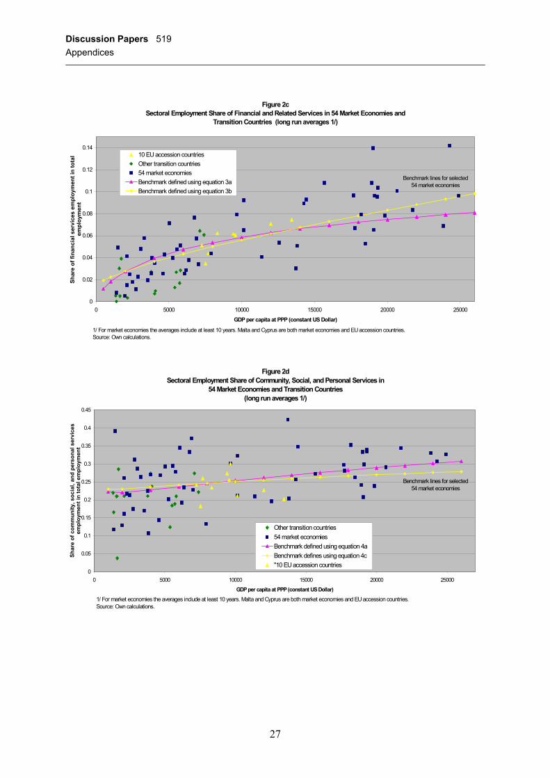
Discussion Papers 519 Appendices
27
Figure 2cSectoral Employment Share of Financial and Related Services in 54 Market Economies and
Transition Countries (long run averages 1/)
0
0.02
0.04
0.06
0.08
0.1
0.12
0.14
0 5000 10000 15000 20000 25000
GDP per capita at PPP (constant US Dollar)
Shar
e of
fina
ncia
l ser
vice
s em
ploy
men
t in
tota
l em
ploy
men
t
10 EU accession countriesOther transition countries54 market economiesBenchmark defined using equation 3aBenchmark defined using equation 3b
Benchmark lines for selected 54 market economies
1/ For market economies the averages include at least 10 years. Malta and Cyprus are both market economies and EU accession countries.Source: Own calculations.
Figure 2dSectoral Employment Share of Community, Social, and Personal Services in
54 Market Economies and Transition Countries (long run averages 1/)
0
0.05
0.1
0.15
0.2
0.25
0.3
0.35
0.4
0.45
0 5000 10000 15000 20000 25000
GDP per capita at PPP (constant US Dollar)
Shar
e of
com
mun
ity, s
ocia
l, an
d pe
rson
al s
ervi
ces
empl
oym
ent i
n to
tal e
mpl
oym
ent
Other transition countries54 market economiesBenchmark defined using equation 4aBenchmark defines using equation 4c"10 EU accession countries
Benchmark lines for selected 54 market economies
1/ For market economies the averages include at least 10 years. Malta and Cyprus are both market economies and EU accession countries.Source: Own calculations.

Discussion Papers 519 Appendices
28
Appendix E: Figures 3a-3d
Figure 3aAdjustment path of the Employment Share of Agriculture in Eastern European new EU member
countries and EU accession candidates during transition 1/
0.00
0.05
0.10
0.15
0.20
0.25
0.30
0.35
0.40
5000 7000 9000 11000 13000 15000
GDP per capita at PPP (constant US Dollar)
Shar
e of
agr
icul
tura
l em
ploy
men
t in
tota
l em
ploy
men
t
Benchmark for market economies defined on the basis of estimated
equation 1e
1/ The small squares give the last available year 2001. The lines that lead to the squares show the evolution of the employment share with each dot representing one consecutive yearly observation.Source: Own calculations.
Poland, 2001
Czech Republic, 2001
Estonia, 2001
Hungary, 2001
Latvia, 2001Lithuania, 2001
Slovakia, 2001Slovenia,
2001
Benchmark for market economies defined on the basis of estimated
equation 1b
Bulgaria, 2001
Romania, (2001=42%)
Figure 3bAdjustment path of the Employment Share of Manufacturing in Eastern European new EU member
countries and EU accession candidates during transition 1/
0.10
0.15
0.20
0.25
0.30
0.35
0.40
4000 6000 8000 10000 12000 14000 16000
GDP per capita at PPP (constant US Dollar)
Shar
e of
man
ufac
turin
g em
ploy
men
t in
tota
l em
ploy
men
t
Benchmark line defined using estimated panel equation 2e
1/ The squares give the last available year 2001. The lines that lead to the squares show the evolution of the employment share with each dot representing one consecutive yearly observation.Source: Own calculations.
Czech Republic, 1992-2001
Slovenia, 1993-2001
Slovakia, 1994-2001
Poland, 1990-2001
Lithuania, 1997-2001
Latvia, 1990-2001
Hungary, 1991-2001
Estonia, 1998-2001Benchmark line defined using estimated panel equation 2a
Bulgaria, 1990-2001
Romania, 1990-2001
Discussion Papers 519 Appendices
29
Figure 3cSectoral Employment Share of Financial Services, Real Estate, and Related Services
in Eastern European new EU member countries and EU accession candidates during transition 1/
0.01
0.02
0.03
0.04
0.05
0.06
0.07
0.08
0.09
0.10
5000 7000 9000 11000 13000 15000
GDP per capita at PPP (constant US Dollar)
Shar
e of
fina
ncia
l ser
vice
s em
ploy
men
t in
tota
l em
ploy
men
t
1/ The squares give the last available year 2001. The lines that lead to the squares show the evolution of the employment share with each dot representing one consecutive yearly observation.Source: Own calculations.
Benchmark line defined using estimated panel equation 8b
Benchmark line defined using estimated panel equation 8a
Czech Republic, 1992-2001
Estonia, 1989-2001 Hungary, 1991-2001
Slovenia, 1993-2001
Latvia, 1990-2001
Lithuania, 1997-2001
Poland, 1990-2001
Slovakia, 1994-2001
Bulgaria, 1990-2001
Romania, 1990-2001
Figure 3dSectoral Employment Share of Community, Social, and Personal Services in
in Eastern European new EU member countries and EU accession candidates during transition 1/
0.09
0.14
0.19
0.24
0.29
5000 7000 9000 11000 13000 15000
GDP per capita at PPP (constant US Dollar)
Shar
e of
com
mun
ity, s
ocia
l, an
d pe
rson
al s
ervi
ces
empl
oym
ent i
n to
tal e
mpl
oym
ent
1/ The squares give the last available year 2001. The lines that lead to the squares show the evolution of the employment share with each dot representing one consecutive yearly observation.Source: Own calculations.
Benchmark line defined using estimated panel equation 9c
Benchmark line defined using estimated panel equation 9a
Czech Republic, 1992-2001Estonia, 1989-2001
Hungary, 1991-2001
Slovenia, 1993-2001
Latvia, 1990-2001
Lithuania, 1997-2001
Poland, 1990-2001
Slovakia, 1994-2001
Romania, 1990-2001
Bulgaria, 1990-2001

Discussion Papers 519 Appendices
30
Appendix F: Figures 4a-4i
Figure 4aAdjustment path of the Employment Share of Agriculture in Poland:
Actuals and Forecasts 1990-2015 1/
0.00
0.05
0.10
0.15
0.20
0.25
6000 8000 10000 12000 14000 16000GDP per capita at PPP (constant US Dollar)
Shar
e of
agr
icul
tura
l em
ploy
men
t in
tota
l em
ploy
men
t
1/ The last available year 2001 is indicated by a square. The lines show the evolution of the employment share with each dot representing one consecutive yearly observation until 2015 in the ex-ante forecasts. The latter assume annual per capita real GDP growth of 4.5% starting in 2004. Additional assumptions are explained in the text.Source: Own calculations.
Poland, actuals, 1990-2001
Forecast based on Equation 1a(1990-2015)
Forecast based on Equation 1e(1996-2015)
Dotted line: potential evolution during 2002-2015
2001 2015
Figure 4bAdjustment path of the Employment Share of Agriculture in Romania:
Actuals and Forecasts 1990-2015 1/
0.00
0.05
0.10
0.15
0.20
0.25
0.30
0.35
0.40
0.45
4500 5500 6500 7500 8500 9500 10500
GDP per capita at PPP (constant US Dollar)
Shar
e of
agr
icul
tura
l em
ploy
men
t in
tota
l em
ploy
men
t
1/ The last available year 2001 is indicated by a square. The lines show the evolution of the employment share with each dot representing one consecutive yearly observation until 2015 in the ex-ante forecasts. The latter assume annual per capita real GDP growth of 4.5% starting in 2004. Additional assumptions are explained in the text.Source: Own calculations.
Forecast based on Equation 1e(1996-2015)
Forecast based on Equation 1a(1990-2015)
Romania, actuals,1985-2001
Dotted line: potential evolution up to 2015
2001 2015

Discussion Papers 519 Appendices
31
Figure 4cAdjustment path of the Employment Share of Manufacturing in Estonia
Actuals and Forecasts 1993-2015 1/
0.11
0.13
0.15
0.17
0.19
0.21
0.23
0.25
0.27
6000 8000 10000 12000 14000 16000 18000 20000
GDP per capita at PPP (constant US Dollar)
Shar
e of
man
ufac
turin
g em
ploy
men
t in
tota
l em
ploy
men
t
1/ The last available year 2001 is indicated by a square. The lines show the evolution of the employment share with each dot representing one consecutive yearly observation until 2015 in the ex-ante forecasts. The latter assume annual per capita real GDP growth of 4.5% starting in 2004. Additional assumptions are explained in the text.Source: Own calculations.
Forecast based on Equation 2e(1996-2015)
Forecast based on Equation 2a(1992-2015)
Estonia, actuals, 1989-2001
Dotted line: potential evolution up to 2015
2001 2015
Figure 4dAdjustment path of the Employment Share of Manufacturing in the Czech Republic:
Actuals and Forecasts 1993-2015 1/
0.15
0.17
0.19
0.21
0.23
0.25
0.27
0.29
0.31
10000 12000 14000 16000 18000 20000 22000 24000
GDP per capita at PPP (constant US Dollar)
Shar
e of
man
ufac
turin
g em
ploy
men
t in
tota
l em
ploy
men
t
1/ The last available year 2001 is indicated by a square. The lines show the evolution of the employment share with each dot representing one consecutive yearly observation until 2015 in the ex-ante forecasts. The latter assume annual per capita real GDP growth of 4.5% starting in 2004. Additional assumptions are explained in the text.Source: Own calculations.
Forecast based on Equation 2e(1996-2015)
Forecast based on Equation 2a(1993-2015)
Czech Republic, actuals, 1992-2001
Dotted line: potential evolution up to 2015
2001 2015

Discussion Papers 519 Appendices
32
Figure 4eAdjustment path of the Employment Share of Manufacturing in Poland:
Actuals and Forecasts 1990-2015 1/
0.18
0.19
0.20
0.21
0.22
0.23
0.24
0.25
0.26
6000 8000 10000 12000 14000 16000
GDP per capita at PPP (constant US Dollar)
Shar
e of
man
ufac
turin
gem
ploy
men
t in
tota
l em
ploy
men
t
1/ The last available year 2001 is indicated by a square. The lines show the evolution of the employment share with each dot representing one consecutive yearly observation until 2015 in the ex-ante forecasts. The latter assume annual per capita real GDP growth of 4.5% starting in 2004. Additional assumptions are explained in the text.Source: Own calculations.
Forecast based on Equation 2a(1990-2015)
Forecast based on Equation 2d(1996-2015)
Poland, actuals(1990-2001)
2001 2015
Dotted line: potential evolution up to 2015
Figure 4fAdjustment path of the Employment Share of Financial Services, Real Estate, and Related Services in the Czech
Republic: Actuals and Forecasts 1992-2015 1/
0.04
0.05
0.06
0.07
0.08
0.09
0.10
0.11
0.12
10000 12000 14000 16000 18000 20000 22000 24000
GDP per capita at PPP (constant US Dollar)
Shar
e of
Fin
anci
al S
ervi
ces
empl
oym
ent i
n to
tal e
mpl
oym
ent
Forecast based on Equation 3c (1992-2015)
Forecast based on Equation 3a (1994-2015)
Czech Republic, actuals, 1992-2001
Dotted line: potential evolution up to 2015
1/ The last available year 2001 is indicated by a square. The lines show the evolution of the employment share with each dot representing one consecutive yearly observation until 2015 in the ex-ante forecasts. The latter assume annual per capita real GDP growth of 4.5% starting in 2004. Additional assumptions are explained in the text.Source: Own calculations.
2001 2015

Discussion Papers 519 Appendices
33
Figure 4gAdjustment path of the Employment Share of Financial Services, Real Estate, and Related Services in Hungary:
Actuals and Forecasts 1991-2015 1/
0.04
0.05
0.06
0.07
0.08
0.09
0.10
0.11
0.12
8000 10000 12000 14000 16000 18000 20000 22000
GDP per capita at PPP (constant US Dollar)
Shar
e of
Fin
anci
al S
ervi
ces
empl
oym
ent i
n to
tal e
mpl
oym
ent
Forecast based on Equation 3c (1996-2015)
Forecast based on Equation 3a (1991-2015)
Hungary, actuals, 1991-2001
Dotted line: potential evolution up to 2015
1/ The last available year 2001 is indicated by a square. The lines show the evolution of the employment share with each dot representing one consecutive yearly observation until 2015 in the ex-ante forecasts. The latter assume annual per capita real GDP growth of 4.5% starting in 2004. Additional assumptions are explained in the text.Source: Own calculations.
2001 2015
Figure 4hAdjustment path of the Employment Share of Financial Services, Real Estate, and Related Services in Slovenia:
Actuals and Forecasts 1993-2015 1/
0.05
0.07
0.09
0.11
0.13
0.15
0.17
0.19
11000 13000 15000 17000 19000 21000 23000 25000 27000 29000
GDP per capita at PPP (constant US Dollar)
Shar
e of
Fin
anci
al S
ervi
ces
empl
oym
ent
in to
tal e
mpl
oym
ent
Forecast based on Equation 3c (1997-2015)
Forecast based on Equation 3a (1993-2015)
Slovenia, actuals, 1993-2001
Dotted line: potential evolution up to 2015
1/ The last available year 2001 is indicated by a square. The lines show the evolution of the employment share with each dot representing one consecutive yearly observation until 2015 in the ex-ante forecasts. The latter assume annual per capita real GDP growth of 4.5% starting in 2004. Additional assumptions are explained in the text.Source: Own calculations.
2001 2015

Discussion Papers 519 Appendices
34
Figure 4iAdjustment path of the Employment Share of Community, Social, and Personal Services in Poland:
Actuals and Forecasts 1990-2015 1/
0.17
0.19
0.21
0.23
0.25
0.27
0.29
6000 8000 10000 12000 14000 16000GDP per capita at PPP (constant US Dollar)
Shar
e of
Com
mun
ity, S
ocia
l, an
d Pe
rson
al S
ervi
ces
empl
oym
ent
in to
tal e
mpl
oym
ent
Forecast based on Equation 4c(1996-2015)
Forecast based on Equation 4a(1990-2015)
Poland, actuals(1990-2001)
Dotted line: potential evolution during 2002-2015
1/ The last available year 2001 is indicated by a square. The lines show the evolution of the employment share with each dot representing one consecutive yearly observation until 2015 in the ex-ante forecasts. The latter assume annual per capita real GDP growth of 4.5% starting in 2004. Additional assumptions are explained in the text.Source: Own calculations.