Downturn LGD: flexible and regulatory consistent … · 2018-01-12 · Downturn LGD: flexible and regulatory consistent approaches Page 2 In the Italian banking context, the most

Downturn LGD: flexible and regulatory consistent approaches Page 1

Downturn LGD: flexible and regulatory consistent approaches*

Alessandro Turri, Risk Control Unit, Banca Popolare di Sondrio

Fabio Salis, Head of Convalida and Data Quality Unit, Cariparma – Gruppo Credit Agricole

Abstract

To identify the downturn LGD, an essential role is played by the banks: they have to determine the business cycle used to find the possible negative

relation between default and recovery rates. To attain regulatory validation, the methodological framework has to be accurate, sustainable and

applied to qualitative robust databases. The simplicity of integration of the downturn corrective in the estimates, also for managerial purposes,

should not be overlooked. Starting from multivariate structural models of economic series, it is possible to derive an identification process for the

impacts of the extracted business cycle on the recoveries and on the determinants of danger rates used to recalibrate the insolvency definition to

the regulatory framework. The result is a proposal of organic, modular approach, that led to the production of regulatory coherent LGD estimates.

1. Introduction

An extremely important element in the recent debate on loss given default (LGD) is the progressive

overcoming of the classic assumption of independence between that rate and probability of default (PD)

that still characterizes the Basel II regulatory framework. Several empirical studies1 have found that, in

presence of recessive phases (downturns) characterized by higher default rates, the values of recovery

rates (complement to the unit of the LGD) are significantly lower because of the reduction of counterparts’

asset value. Therefore, it appears to manifest an inverse correlation between recovery rates and the

systematic risk of the economy. This evidence has important consequences for a correct estimate of credit

risk capital requirements. The models that assume independence between PD and LGD do not appear

adequate, systematically leading to underestimate the necessary capital in adverse macro-economic

conditions and to emphasize pro-cyclical effects already embedded in the regulatory models2. These

empirical findings have resulted, from a regulatory point of view, in the introduction within that

framework3 of the concept of downturn LGD (DLGD). Such DLGD is used in the regulatory functions to

obtain prudential estimates of absorbed capital. The Bank of Italy attributes to the banks the responsibility

of the determination of business cycle and of the connected recessive phases. It is necessary to

demonstrate that the systematic risk of the economy has to be considered within the “relevant factors”

that influence the LGD expected values. The bank must certify the inverse relation between default and

recovery rates by mean of specific analyses based on historical data.

* This article contains only the opinions of the authors and not of the companies with which they serve. The article was written and revised jointly

by the two authors. The paragraphs can however be divided by core competency as follows: 1st, 2nd Salis, 3rd, 4th & 5th Turri, 6th & 7th jointly. 1 Cfr. e.g. Altman et al. (2005); Hu and Perraudin (2002)

2 Altman, Resti and Sironi (2002)

3 Cfr. Banca d’Italia (2006, Titolo II, Parte Seconda, Sez.. IV, Par.2.3)


In the Italian banking context, the most widespread methodology for estimating LGD is based on an

actuarial approach (workout LGD – discount of all the cash flows registered from the passage to default to

the closing of the position). Beyond the technical difficulties related to the preparation of the data set for

the estimates, we underline that LGD values deriving from such methodology can naturally be far away

from the punctual situations of the business cycle. This is especially true in a context, like that Italian one,

characterized by lenghty recovery procedures .

An additional element of complexity in the Italian context is derived from the peculiar difference of default

definitions used in the development of the LGD models. For this purpose, recovery data on non-performing

loans (typically “an absorbent” state) are commonly used, since they are often characterized by greater

reliability and temporal depth with respect to data on “less extreme” and “reversible” states of default (i.e.

the so called “incagli” – watchlist loans - and the 180 “not technical” past dues). The LGD estimates based

on non-performing loans are usually recalibrated using appropriate danger rates, that on one side express

the probability to fall into insolvency in a state of default “less absorbent” and from the other side measure

the probability to come back “in bonis” from that state. The use of danger rates involves the necessity to

verify punctually, in the spirit of the Regulation, the existence of an inverse relation between the bank’s

danger rates level and a series of factors - some of which variable in relation to the course of the economy

(at a general or sector level). Furthermore, in the estimation of the DLGD it is important to consider the

recessive conditions that are relevant for the estimation of danger rates. We can hence conclude that the

DLGD estimate can be seen as a combination of a DLGD estimated on bad loans (or bad loans and watchlist

loans if the we have sufficient data), and an estimation of a downturn danger, DDR.

A bank that wants to develop a LGD system potentially coherent with the Regulation in terms of DLGD, has

to understand his positioning regarding the above mentioned issues. The solution will be bank-specific and

the level of complexity dependent from the available information. In the decision, a key role will be played

by the methodology adopted for the identification of recessive phases. During this current persistent

period of economic crisis, also the role of the internal validation function in the identification process of a

DLGD regulatory compliant is crucial. This function has to verify, independently from the model

development function, the conservativeness and the soundness of different methodological choices made.

A pivotal requirement for an effective validation analysis is the availability of a rigorous and complete

documentation, that contains all the development phases of the methodological framework. For instance,

the rationale for the definition of an appropriated recessive phase for each homogenous portfolio of

activity, or the statistical analyses for the identification of a possible inverse relation between default and

recovery rates must be described. Moreover, the determination of the operating modalities used to

incorporate the downturn effect in the workout LGD estimates, the external (i.e. the historical series of


macroeconomic factors) and internal data sets (i.e. the internal recovery rates for customer’s segment,

technical form, …) utilized must be clear. It is even appropriate to mention the external benchmarks

underlying the assumption of key choices (i.e. market parameters for the calculation of an interest rate

spread adjusted for the downturn effect).

After discussing some issues concerning the discount of the historical flows of recoveries in a workout LGD

perspective (par. 2), we will present a methodology (par. 3) to build an index for the business cycle (i.e.

creation of a synthetic indicator to identify the recessive phases). Moreover, we will verify the correlation

effects between default and recovery rates, taking into account also danger rate models (par. 4). In

paragraph 5, an organic, modular, manageable and upgradeable framework to produce LGD estimates will

be defined. Eventually, we will outline some useful considerations in order to lead an accurate internal

validation analysis (finalized to test the regulatory compliance of the methodological choices adopted) and

a few critical remarks about pro-cyclical effects potentially inherent in the regulatory definition of DLGD

(par. 6).

2. The workout approach

The workout LGD discounts the recovery cash flows, without the recovery costs and without the eventual

increases of the exposure at default. A widespread choice among the Italian banks is to discount flows by

use of the long term rates structure (EURIBOR/IRS) referred to the month and year of passage to default

(backward looking solution) or, alternatively, to the moment of LGD model estimation (forward looking

solution).

From a strictly regulatory point of view, the Regulation seems to request that discount rate has to include

an opportune add-on (a spread-over-market-risk) for the recovery risk implicit in the exposition4. In order

to derive a workout “downturn” LGD, it appears possible to include in the spread-over-market-risk a risk

premium component for the coverage of the recessive phases. As a matter of fact, a higher volatility of the

observed and expected yields is then found. For instance, if we estimate - through G.A.R.C.H. models - the

relation between the market index volatility and the risk premium, it’s possible to determine some

prudential corrections of the risk premium, in comparison with the higher volatility embedded in the

recessive phases. In such a way, the DLGD is given from the discounting of the cash flows using the new

rate. This methodological approach does not explicit a direct link with the business cycle, because it does

not include explicative variables in the model but defines the adverse cycle effect on the recoveries basing

4 Banca d’Italia (20006,Titolo II, Parte Seconda, Sez.. IV, Par.2): “… il calcolo del valore attuale deve riflettere sia il valore monetario del tempo sia il

rischio insito nella volatilità dei flussi di recupero mediante l’individuazione di un premio al rischio adeguato; solo in assenza di incertezza nel

recupero (ad esempio se i recuperi provengono da depositi in contanti) il calcolo del valore attuale può riflettere il solo valore monetario del tempo”

[“… the actual value must reflect both the monetary value of time and the risk of volatility of the flows by mean of an appropriate risk premium. Only

in absence of uncertainty over recoveries (e.g. when they come from cash deposits) the actual value can reflect just the very value of time”]


only on market indices, through the observation of their volatility. From a methodological point of view, we

prefer more flexible solutions respect to the one proposed above.

3. Identifying a reference business cycle

The study of business cycles necessarily starts from their measurement and the definition of different

phases. The well known definition of Burn and Mitchell (1946) define the business cycle as composed by

“expansions occurring at about at the same time in many economic activities, followed by similarly general

recessions, contractions and revivals which merge into the expansion phase of the next cycle”. This

sequence of changes is recursive but not periodical. Thus there are two main characteristic: first, the

presence of similarities in the dynamic of the series; second the continuous reversibility of economic

fluctuations, even if not at exactly precise intervals. The very presence of these co-movements implies that

to correctly define the cycle we must jointly examine different economic series. Furthermore we reveal that

the proposed definition specifies the exact nature of the economic fluctuations, but nonetheless the

movements in economic activity may take diversified duration and characteristics. Theoretically is possible

to distinguish between long-period (structural) components and short (medium)-period ones. The latters

are, strictly speaking, the cycles we are looking for. Practically, for Burn and Mitchell the distinction was still

cumbersome due to the lack of adequate techniques to separate them.

Starting from the ‘60s, following a period of pronounced and uninterrupted trend of growth in the main

economic variables, a wide set of techniques were developed to extract those components from the series.

That has led to new definition of business cycles in terms of deviations from a specified trend – the so

called deviation cycle – or in terms of movements around a growth rate – the so called growth cycle.

Anyhow starting with the works of Beveridge and Nelson (1981) and Nelson and Plosser (1982) the cycle

was more precisely defined as the residual part of a time series after the extraction of a permanent

component (stochastic or deterministic). While the trend represents the non-stationary component, the

business cycle is constrained to stationarity, moving around its long period equilibrium level.

All those premised, to correctly analyze the business cycle is essential to have long and sound time series

(e.g. quarterly or monthly ones). For instance data from Istat and Bank of Italy may be used, grouped

according to the following drivers of analysis5:

• Macroeconomic variables related to the Italian economic system (household consumption, gross

fixed investments, labour units, wages, GDP, Value Added, Industrial production index, etc.)

• Market variables related to the credit system (default rate for loan facilities6, etc.)

5 Similar to the distinction found in Querci (2007; p.177).

6 The so called “Tassi di decadimento”.


The objective is the identification of an appropriate representative index of the business cycle. From a

general point of view we refer to Burns and Mitchell for its main features:

• It must reflect the co-movements of different and economic relevant time series.

• It must show a tendency to revert (even if not at constant intervals) to a long-period value.

We can conduct the analysis in two distinct phases:

1. A univariate study of the specific time series features is conducted, by structural models7.

2. Afterwards an analysis for the identification of a ”common reference cycle” is pursued by mean of a

multivariate extension of the previous approach8.

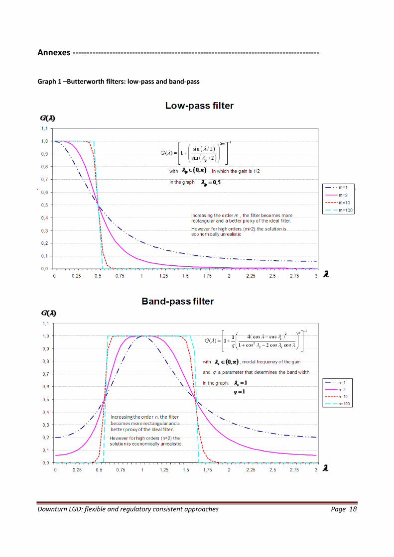
This framework builds upon concepts of spectral analysis and the so-called Butterworth filters, by achieving

a time series decomposition based over different captured frequencies. The construction of those

decomposition filters tries to target to different results:

• An ideal filter characterized by a gain function that is shaped as an index function over a selected

band of frequency.

• A filter that is able to recover stochastic components that are meaningful from an econometric

point of view and useful for forecasting.

It’s not always easy to pursue the correct balance between these two objectives, that are in contrast

among themselves; as a matter of fact, to obtain the perfect approximation of ideal filters stochastic

components with high order of integration are needed. Nevertheless, this is in contrast with the “common-

sense” of econometricians and economists that regards trends of order higher than two or integrated

cycles as unrealistic.

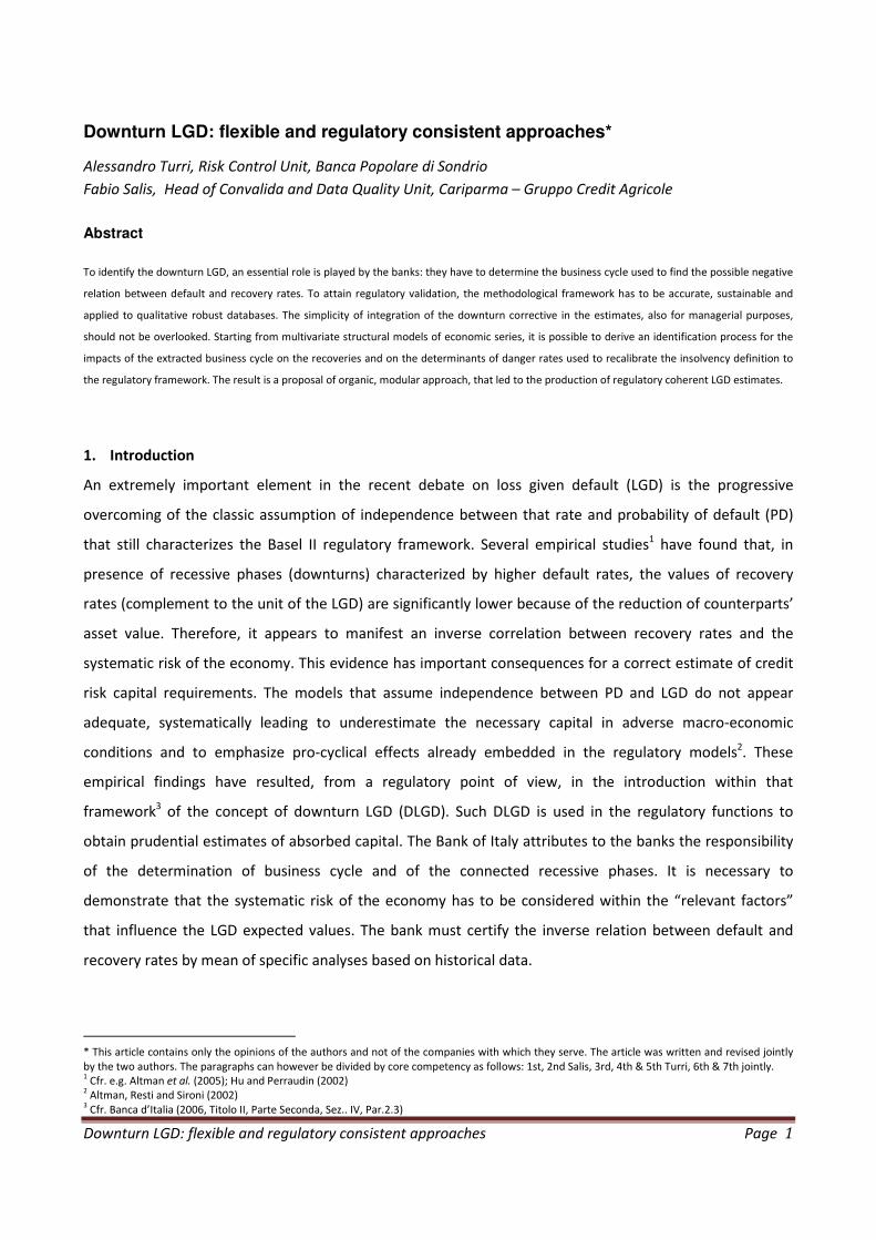
Butterworth filters allow the extraction of both the trend and the cycle from a time series. That is shown in

Graph 1, where we find the low-pass filter, that extracts the low frequency movements, and the band-pass

filter, that separates the average frequencies, typically characterizing the business cycle9.

Limiting for sake of simplicity our argument to already seasonally adjusted time series10

, it’s possible to

break the series in factors in the following way11

:

ttntmty εψµ ++= ,, tε ~ ),0(t

NID εσ Tt ,,1K= (1)

7 Look at Harvey (1989), Harvey and Trimbur (2003) , and Pelagatti (2004).

8 Or, as the regulator impose, more reference cycle indexes distinct for the main class of counterparts/exposures that characterize the activity of the

financial intermediary. 9 The high frequency components are summarized into the disturbs, and, for time series not seasonally adjusted, in possible seasonal terms.

10 But the result is obviously extendible by proper seasonal components.

11 The software STAMP ™ (by OxMetrics ™) has been used for the elaborations. It allows a univariate and multivariate structural time series analysis.

We refer to Koopman & al. (2007) for the statistic exposition here briefly summarized. To this text we refer also for further in-depth analysis

regarding SUTSE multivariate models.


where tm,µ is a stochastic trend (with deterministic level and stochastic slope), tn,ψ is the stochastic cycle

and tε is a white nose; m and n are the trend and cycle order corresponding to the order of the low-pass

filter and the order of the band-pass filter.

The stochastic trend component is specified as:

tttt ηβµµ ++= −− 11 tη ~ ),0(2

ησNID (2)

ttt ςββ += −1 tς ~ ),0(2

ςσNID (3)

where tβ is the slope (gradient) of the trend tµ (a facultative component) and ttt ςηε ,, are mutually

uncorrelated white noises. By the assumption of a fixed level, in (2) tη is null, due to 2

ησ = 0.

The stochastic cycle component is specified as:

( ) ( )

1

*( ) *( ) *

1

cos sin

sin cos

n nc ct t t

n nc ct t t

ψ

λ λψ ψ κρ

λ λψ ψ κ−

−

= + −

Tt ,,1K= (4)

where (n) is the cycle order; ψρ , with 10 ≤< ψρ , is the damping factor; cλ is the frequency, in radians, in

the range πλ ≤≤ c0 ; tκ and *

tκ are two mutually uncorrelated NID disturbances with zero mean and

common variance 2

κσ . The period of the cycle, one of the factors of utmost interest in our decomposition

of the time series, is set to cλπ /2 .

Consistently to economic logic, the parameters regarding the order of integration of the low-pass filter and

pass-band filter are so fixed:

• m = 2, for the trend (i.e. an integrated random walk)

• n = 2, for the cycle (i.e. a stochastic cycle of 2nd order)

Only where was considered appropriate (usually in cases with possible high frequency cycles), a m=1 trend

(random walk) was used in order to guarantee that the pass-band filter hold back also a part of the

frequencies that are typical of long-period cycles. The business cycles of interest usually identify

fluctuations in the range of 1.5-8 years, which correspond to power spectrum in the interval [0.20π; 1.05π].

Cyclical behaviour outside this range, whenever detected, is considered not relevant for our ends.


After the univariate analyses is possible to jointly examine the characteristics of the discovered cycles. First,

we proceed by mean of homogeneous sub-categories of variables. Second, we thoroughly investigate the

connection among the most interesting variables. Thus doing we come from a long-list to a short-list of

significant variables that stand for inclusion in a reference cycle index.

For the second stage of multivariate analysis is possible to use SUTSE (Seemingly unrelated time series

equations) models. They present a logical structure quite similar to the one already examined for the

univariate case. However, here there is a vector of observations dependent by unobserved components

vectors. The different series examined are linked by the correlations of their disturbances. Given a set of

economic time series, it’s particularly interesting the possibility to extract a cycle (or more cycles) with

similar characteristics: the same frequency, cλ , and the same damping factor, ρ . These cycles are called

“similar cycles”. Furthermore, the disturbance correlation matrix can be less than full rank (so called

“common factors model”) thus reducing the numbers of parameters that must be estimated and

simplifying the derivation of results. The identification of a common cycle among time series (i.e. the

discovery of different cycles exactly proportional) has the natural interpretation of a synthetic index

representative of the business cycle derived by the underlying factors.

In order to reduce the complexity of the problem and the relating information processing time, in the

multivariate analysis we limited our focus to the joint consideration of the variables that the univariate

stage pointed out as relevant. Nevertheless, we maintained a limited number of time series for each area of

economic/financial meaning.

In a first stage we conducted a similar cycle analysis without imposing “ex-ante” common cycles, but just a

few constraints over the disturbance matrix of the trend and seasonal component. In a second stage,

having discovered by the unconstrained analysis the emergence of a natural common cycle, we repeated

the process of model derivation by imposing in advance the constraint of a common cycle presence.

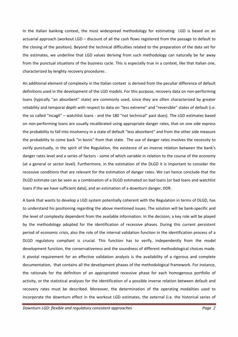
Alternative models were estimated for different exposure classes. Yet they revealed not to be significantly

different from a general one (Graph 2). Thus, for sake of simplicity, we adopted that one as the “reference

cycle”. The variable INDEXCYCLE shows for the Italian economy a behaviour well in line with most of the

empirical external evidences and identifies 7 recessionary periods of different intensity: …-1990(3);

1992(2)-1993(3); 1995(3)-1996(4); 1998(1)-1999(2); 2001(1)-2002(3) ; 2004(1)-2005(1); 2007(2)-….


4. Does exist an inverse correlation between default and recovery rates?

Given a reference cycle, we proceed to identify a possible inverse relation between defaults and recovery

rates12

. More generally speaking we examine the links between the different phases of the business cycle

and the level of historically observed LGD. We identify the main idiosyncratic factors that influence LGD

within multivariate models. Most of them are categorical ones, thus suggesting the use of generalized

linear models for the analysis of variance. Consistently with the normative rules on the correct definition of

default to be used in the estimate of risk factors, we have hence extended our analysis to include in LGD

also less absorbing state of default as the so-called “incaglio” (watchlist loans) and past due (over 180

days). Starting from a direct estimate on a historical sample of “sofferenze” (non-performing loans), we

later extended it by mean of multivariate models explaining danger rates.

Then, for each model, the possible impact of downturns on the variance of the target variable was tested.

Only the residuals of models with idiosyncratic factors were considered. For instance, the relation between

LGD of “sofferenze” in specific periods and the correspondent phase of business cycle (recession vs.

growth) was closely examined. Three solutions have been explored:

• First, as in previous studies, the association was based on the opening date of default.

Nevertheless, it appears doubtful that, due to the long-lasting length of recovery process in Italy,

the macroeconomic conditions present at the opening of default are strictly linked with recovery

rates.

• Second, the association was based on the quarter during which the last movement on the position

was observed. This appears sensible since often most recoveries are concentrated in the last

observed movements before the closing of the position.

• Third, we determined a “barycentre of recoveries” for each position. From specific movements in

the sample an average delay respect to the opening date was determined and weighted by the

recovered amounts on the position.

The analyses were done in the three ways13

to make results on macro-economic conditions impact more

sound and documented.

To verify the existence of significant differences in LGD values during recession and growth we first used

test for independent samples to compare the values of the residuals from a regressive model with only

idiosyncratic factors. Since these residuals are often non-normal we used non-parametric tests14

. Then, also

12

Cfr. Banca d’Italia (2006, TIT. II, Parte seconda, SEZ.IV, par.2.1) 13

Anyhow for the danger rates models only the first and second way of association were possible. 14

Mann-Whitney, Moses, Kolmogorov-Smirnov to compare LGD levels during recession and growth. Kruskal-Wallis to analyse the differences

among specific phases of the business cycle (periods defined by using the previously determined reference cycle)


the intensity of the cycle phase was tested by mean of a direct regression with INDECYCLE as explicative

factor: first only on the residuals of previous regression, second (when significant) directly in a revised

model with both idiosyncratic factors and the systemic factor.

Generally speaking we can conclude that most of LGD variability is explained by counterpart or credit line

specific factors. In comparison the macroeconomic factors – when significant - have a more limited effect in

absolute term. Even if cannot be denied that the inclusion of INDECYCLE in the models, whereas statistically

significant, led to great R2 improvements in relative terms. For example, according to the methodological

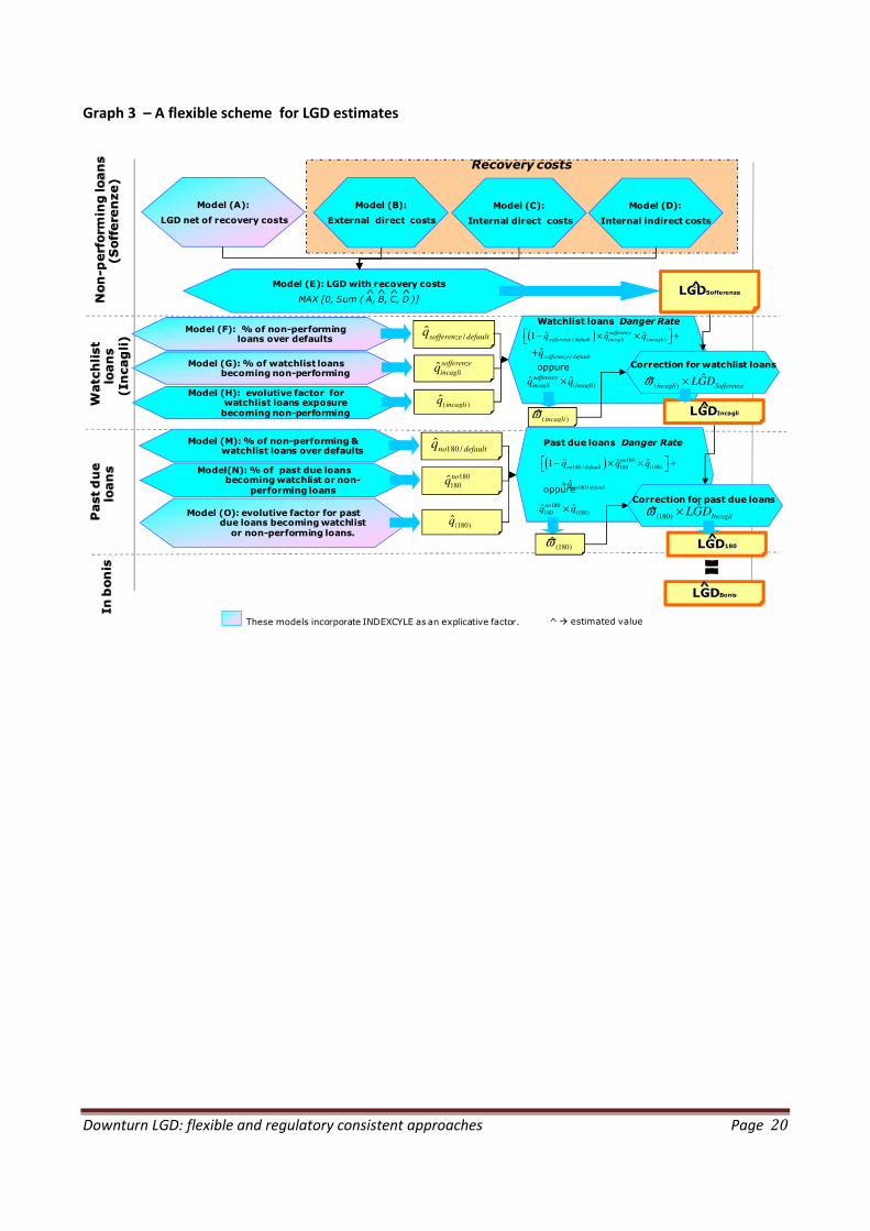
framework of the next paragraph (Graph 3) we found that the inclusion of the reference cycle index among

the predictors led to the following R2 relative increments compared to correspondent models with only

idiosyncratic factors: 17.3% in (A), 2.8% in (F), 7.0% in (G) and 23.6% in (O). For all that a prudential

inclusion of INDEXCYCLE in the model is wise, whereas it turns out to be significant and with a coefficient

consistent with regulator’s expectations. This done a DLGD may be easily derived by replacing the historical

value of reference cycle with a synthetic measure of its value during picked out recessions. For example:

� we can distinguish 2 phases of the cycle, recession and growth, and set an appropriate percentile

(e.g. 25°) of the INDEXCYCLE in the recessive phases as a reference value to substitute into the

models;

� otherwise we identify 4 phases: “growth under the trend”, “growth above the trend”, “recession

under the trend” and “recession above the trend”; then we fix the value for DLGD estimate to the

average or median one observed during “recession under the trend” phases.

Both methodologies appear in line with regulator’s suggestions without leading to overly prudential

corrective factors that may improperly affect the estimates (cfr. paragraph 6 for further investigation on

this problem)15

.

5. A modular scheme for LGD

The study of the connection between recovery rates and default rates in the Italian economic environment

has a peculiar element of complexity: the difference of the normative definition of default from the

concept commonly used when estimating LGD models. Here the choice is often for the use of discounted

cashflows of credits in “sofferenza” ( typically an irreversible state), a narrower concept than the Basle 2

one (that comprises also “incagli” and past due loans).

15

For the themes of paragraphs 3 and 4 see also Turri (2008).


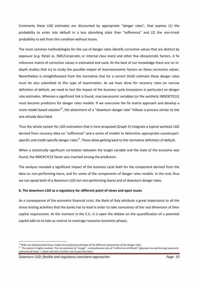
Commonly these LGD estimates are discounted by appropriate “danger rates”, that express (1) the

probability to enter into default in a less absorbing state than “sofferenza” and (2) the non-trivial

probability to exit from this condition without losses.

The most common methodologies for the use of danger rates identify corrective values that are distinct by

exposure (e.g. Retail vs. SME/Corporate; or internal class ones) and other few idiosyncratic factors. A fix

reference matrix of corrective values is estimated and used. At the best of our knowledge there are no in-

depth studies that try to study the possible impact of macroeconomic factors on these corrective values.

Nevertheless is straightforward from the normative that for a correct DLGD estimate these danger rates

must be also submitted to this type of examination. As we have done for recovery rates on narrow

definition of default, we need to test the impact of the business cycle (recessions in particular) on danger

rate estimates. Whereas a significant link is found, macroeconomic variables (or the synthetic INDEXCYCLE)

must become predictors for danger rates models. If we overcome the fix matrix approach and develop a

more model based solution16

, the attainment of a “downturn danger rate” follows a process similar to the

one already described.

Thus the whole system for LGD estimation that is here proposed (Graph 3) integrate a typical workout LGD

derived from recovery data on “sofferenze” and a series of models to determine appropriate counterpart-

specific and credit-specific danger rates17

. These allow getting back to the normative definition of default.

When a statistically significant correlation between the target variable and the state of the economy was

found, the INDEXCYCLE factor was inserted among the predictors.

The analysis revealed a significant impact of the business cycle both for the component derived from the

data on non-performing loans, and for some of the components of danger rates models. In the end, thus

we can speak both of a downturn LGD (on non-performing loans) and of downturn danger rates.

6. The downturn LGD as a regulatory tie: different point of views and open issues

As a consequence of the economic-financial crisis, the Bank of Italy attribute a great importance to all the

stress testing activities that the banks has to lead in order to take conscience of the real dimension of their

capital requirement. At the moment in the E.U. it is open the debate on the quantification of a potential

capital add-on to take as reserve to coverage recessive economic phases.

16

With use of generalized linear models for producing estimates of the different components of the danger rates. 17

The system is highly modular. First an extension to “incagli” - comprehensive also of “sofferenze rettificate” (adjusted-non performing loans) and

restructured loans - is done and next a further one to past due loans.


One of the most common ways to reach this goal, is to identify and quantify this capital surplus working on

risk parameters: the inputs of the regulatory capital function (PD, EAD and LGD). Even if, from a strict

interpretation of the Regulation, Bank of Italy request to the banks to stress the PDs and to the control

functions to verify the robustness of the adopted methodology, the conservativeness of the scenarios and

the underlying hypotheses of correlation, in the definition of the process of downturn LGD calculation, the

Regulator also states that “the adverse economic conditions may coincide with those adopted for the

conduction of the stress testing” 18

. Thus, a strict link between PD stress testing and downturn LGD is set.

The underlying regulatory idea is to guarantee a greater coherence between the various framework of

calculation of Basel 2 risk parameters. Moreover, we observe that the potential capital savings connected

to the passage from the Foundation approach (with regulatory LGD at 45%) to AIRB Method (with LGD

internally estimated) are mainly depending from LGD component, because of the shape of the regulatory

capital curve (Gordy curve). In fact, while the PD enters not linearly in the calculation (it is an input of the

cumulative distribution function of losses and of the correlation) and therefore its variation involves a

mediated impact on capital, on the contrary the LGD is introduced linearly. Thus any LGD reduction

involves the same proportional effect in terms of smaller capital absorption.

Such thematic was also discussed in a meeting between the Bank of Italy Governor and the main

bankers of the system. In such context (Bank of Italy, 2009), among the several arguments dealt (with a

specific focus on the strategies of patrimonial strengthening), the big attention that the Regulator

attributes to the impact of various stress scenarios on the banks’ expected losses has been confirmed.

The hypothetical scenarios are divided in a base one, in which we register the expected losses

embedded in the banks’ portfolios (with a LGD of 35%) and three adverse, with higher losses (with a

LGD of 45%).

Given the remarkable impacts in terms of patrimonial absorptions that a not precautionary downturn

LGD estimate could involve, in our opinion it is very important the role carried out by an independent

function (i.e. the internal validation unit) in the monitoring phase of the conservativeness and

robustness of the various methodological choices made up under development. Often such activity is

much more difficult because of a methodological documentation not always complete.

Before carrying out the controls on the various steps of determination of the downturn effects and of

their incorporation in the workout LGD model, it is essential to make a serious analysis of data quality

on the inputs of the calculation model. Usually the workout LGD models are based on the cash flows

(recoveries and costs) registered on the positions closed in a non-performing loan status. This choice could

18

Banca d’Italia (2006, Titolo II , Cap. I , Sez. IV).


simplify the analyses respect to situations in which the developer decide to use also the cash flows

regarding watchlist loans (“incagli”) and the 180 days past dues. As a matter of fact, in these latter cases

the variety and complexity of the IT procedures to investigate greatly complicate the verification activities.

In our personal experience - that reflects the history of the majority of the Italian banks - the presence of

merging among banks has rendered these controls extremely articulate and laborious, also because

reduction costs’ problems have prevented a rigorous data storing of closed positions at the moment and/or

before the merging.

The choice commonly used to estimate a LGD model on position closed in “sofferenza” and to recalibrate it

on default status “less absorbent” (“incagli” and 180 days past dues) involves a LGD reduction that, in some

way, could be partially counterbalanced from the downturn component (the idea underlying is not so far

from that expressed during the meeting among Italian bankers and the Regulator). However often this

does not happen, partially because of the practical difficulties to determine a robust correlation

between default and recovery rates, basing on historical series not always reliable and sometimes

incomplete. Thus, still a problem of data quality! For us, a crucial role in the development phase of a

compliant LGD model is the dimension and the quality of the dataset. As an example, it is difficult to

answer positively to the Regulation when it request “to define an appropriate recessive phase for

every homogenous portfolio within each jurisdiction” because often we have not the data separated

for each portfolio (i.e. there could be a lack of data concerning the regulatory segmentation of the PD)

or for jurisdiction (e.g. the details of the economic sectors) because of information not always

separable. Whereby possible, as in the approach introduced in par.3, the development of alternative

models for different customer’s segments does not take always results meaningfully different from the

baseline (not subdivided for segments).

The proposed methodological solution is very interesting for two reason:

- first, the modality of determination of the economic cycle, through the utilization of many

explicative variables (macroeconomic and market variables). The focus only on a unique

macroeconomic variable (i.e. G.D.P. or a variable not properly “macro” as Bank of Italy default rate)

could involve potential “bias” in the identification process of the cycle;

- second, it is interesting the application of the correlation analyses of the dependent variables not

only on “bad loans” positions but also on danger rate models.

Concerning the analyses of the eventual inverse relation between default and recovery rates, the relevant

problem is connected to the definition of the temporal lag between the cyclical phase and the loss rate


that, usually for non-performing loans, is based on the observation of the recoveries registered in a multi-

annual temporal span.

At the moment, even in the absence of a universally accepted solution, the approach introduced at par. 4

seems the best because it tries to draw conclusion on the subsistence of such relation not just focusing on a

unique default-loss matching rule, but investigating some alternatives. In particular the last proposed rule

(that starting from book/extra-book keeping movements concerning the development sample try to

determine, for each position, the average delay of the recoveries from the opening of the non-performing

loan position) appears the most compliant from a regulatory point of view.

Often, even very articulate methodologies do not allow detection of a "strong" connection between loss

rates and the state of the business cycle by using the available historical time series. First, indeed, it is

necessary to find a statistic significance of the link between macroeconomic variables / conjuncture

synthetic indices and target variables (taking into account appropriate confidence levels, due to the often

small dimension of the samples). Second however, and not least, question arises for which levels of

explained variance of the total historically observed recovery variance (or the behavior of the specific

objective variable, in the event of the models of danger rates), the impact effect on the final LGD estimates

could be considered really “substantial”. As a matter of fact, we recall that, because of the peculiar bimodal

distribution of the recoveries, the level of variance explained by the commonly utilized models is generally

low. Which additional contributions to the variance explained by a model with cycle-related explicative

variable can be ignored without incurring into serious distortions of the “correct risk quantification”? Which

basic components (look at the modular scheme illustrated in par. 5) of the final LGD are impacted by

macroeconomic variables in a significant and sufficiently intense way? The solution of the problem is not

trivial. It is necessary to make considerations on appropriate reference metrics to define the contribution of

explanatory variables in relation with the cycle and also, more generally, on the opportunity cost of

investment for development and maintenance of complex models.

On the one hand it is true that the regulator, for failure in the detection of significant relationships of

recoveries with the business cycle, allow for calculating DLGD as a weighted average of the long-term

observed loss rates. However, on the other hand, we must observe that this translate into a de facto return

of the econometric model to logics that are closer to a simpler look-up table.

The approach to Basel 2 DLGD and its potential pro-cyclical and anti-cyclical aspects deserve some further

consideration, in light of ongoing discussions between the supervisors. Once verified the correlation, the

proposed solution leads to an increase in capital levels during growth phases. Nevertheless, the introduced

cyclical effect is largely asymmetrical. In fact, also in recessions showing intensity equal or smaller than that


implicitly introduced by the downturn corrective corresponding capital reserves will not be released. By

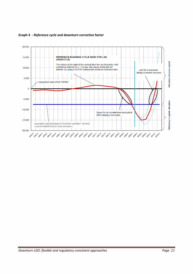
way of explanation let us consider Graph 4 based on real data.

The horizontal line is representative of a level of INDEXCYCLE set for the downturn corrective. The above

curve is instead the reference cycle historically observed and expected in future periods. The descending

sections of the curve, below the zero value, represent recessions, those ascending stages of growth. Adding

the position in relation to the null value (i.e. the level of the trend of the Italian economy) the four cases

already stated at the end of par. 4 arise. For values of the reference cycle (observed or estimated) above

the line of the historically applied downturn level, effects of capital allocation in excess of actual needs

occur, both in case of phases "above the trend", and in case of phases “under the trend”. Only particularly

negative cyclical phases (with INDEXCYCLE levels below the corrective reference value) can generate an

anti-cyclical effect in the application of DLGD. Problematic is the role of the adopted rule in phases “under

the trend” where excess capital allocation takes place. In particular, there is the risk of pro-cyclical effects

of acceleration of the recessions and slowdown of the phases of recovery.

Overall, placing the corrective to levels representative of the most pronounced recessions (such as that just

observed) could exacerbate the effects introduced by the pro-cyclical prudential supervisory framework by

compounding the initial credit crunch and slowing down the next recovery. Conversely, inadequate levels

of the corrective expose banks to unduly underestimate the actual risk faced in times of severe economic

crisis, and to face risk of competitive crowding out compared to competitors that do not use models of

DLGD during the positive phases of the cycle.

So we focus on the delicate problem of determining the appropriate level of the downturn corrective. To

date, this do not find in the consolidated operating practices and regulatory guidelines a solution that

balances among the need for systemic stability, anti-cyclicity and a fair competitive positioning of the

banking players. There seems therefore more robust and viable, in a regulatory view, a methodological

solution within the First pillar (such as those outlined in this paper). This one, subject to the verification of

statistical significance, should incorporate in the econometric estimates of LGD also explanatory variables

(or a synthetic indicator) that 'catch' in some way the presence / absence and relative intensity of a

recessionary period. Nevertheless, then, the actual (or forecasted) values of macroeconomic variables

should be used instead of the prudential downturn values (as mentioned in par . 4). This choice would have

secure benefits, such as improvements of the reliability of the risk-adjusted pricing of credit.

Would remain instead open the possibility to compare these estimates with those obtained in case of

adoption of DLGD in the context of stress testing and, more generally, of the Second Pillar. There, if the

case, by using different levels of conservativeness that take into account, for instance, the lending policies


and the combination of other risks to which the intermediary is subject. At that time you could quantify any

over-allocation of internal capital during good times and moderately negative phases. You could also try to

assess the possible margins of freed capital of the phases under the reference level of the downturn

corrective. This latter anti-cyclical function could even be directly modulated by the Supervisory Authority

within the SREP assessment.

7. Conclusions

We have seen how the supervisory authority, in relation to the issue of DLGD, suggests banks to

independently identify the appropriate reference business cycle, before proceeding against such a

benchmark to verify the real impact of adverse cyclical conditions on the level of recoveries. The level of

autonomy granted to the bank requires the search for a methodological framework for accurate analysis.

This must be combined in an appropriate level of complexity and comprehensibility in compliance with

specific regulatory constraints. Furthermore, it must produce a final solution for LGD consistent with

management needs. Internal and external data bases of proven quality should support the analysis.

The use of structural models for multivariate analysis of macroeconomic time series (SUTSE) seems to

provide an efficient and easily upgradeable solution to the problem of identifying the reference cycle and

for the quantification of its intensity.

As for the check of the impact of recessionary conditions of the business cycle on the levels of LGD, it's

easy to use a synthetic index (derived using SUTSE models): the INDEXCYCLE. This stands as its proxy and

become the candidate explanatory variable to explain the observed variability of recoveries or the objective

variables that are alternatively used in the danger rate models (these used to standardize the definition of

insolvency to the regulatory one).

Faced with a clear and replicable operational plan, which covers the direct integration of a synthetic

indicator in macroeconomic models to estimate the rate of loss in case of insolvency, the main problem

seems to remain the third condition imposed by the Bank of Italy. It is not easy to determine a correct

threshold for the level of significance needed for deciding whether to incorporate the corrective downturn

in the models or, on the contrary, continue to use weighted averages of the long-term observed loss rates.

While the statistical significance of the assumed relationship can often be detected, the more uncertain is

the “substantiality” of the effect, in relation to the problem of proper quantification of risk. Conservative

choices may suggest including the downturn effects in the estimates. In this case, however, problems of

defining the appropriate level of correction introduced remain open. These can lead to very different


solutions in terms of capital absorption, thereby generating potential adverse pro-cyclical effects and an

unfavourable competitive position for the bank.

Therefore, in the absence of clearer regulatory guidance over the "minimal level of substantiality” for the

correlation effect for binding inclusion in a DLGD scheme, it seems to emerge a situation that leads us to

suggest, in a pure First Pillar view, the adoption of explanatory models possibly sensitive to the cycle, but

not directly linked to average reference prudential values. The anti-cyclical management of the estimates of

capital by any additional capital buffer could be left to the stages of stress testing and ICAAP (Second Pillar).

In any case, that is now supported by a unique and consistent framework for LGD analysis.


Bibliography

• Altman E. I., Brady B., Resti A. and Sironi A. (2005), “The Link between Default and Recovery Rates:

Theory, Empirical Evidence, and Implications”, in The Journal of Business, 78: 2203-2228.

• Altman E.I. , Resti A. and Sironi A. (ed.) (2005), “Recovery Risk – The Next Challenge in Credit Risk

Management”, Risk Books, London, UK, March.

• Altman E. I., Resti A. and Sironi A. (2002), “The link between default and recovery rates: effects on

the procyclicality of regulatory capital ratios”, BIS Working Paper No.113, Basle, CH, BIS, July.

• Banca d’Italia (2006), “Nuove disposizioni di vigilanza prudenziale per le banche”, Circolare n° 263,

Rome, Italy, 27 December.

• Banca d’Italia (2009), “L’evoluzione della situazione dei rischi e il patrimonio – Incontro con sei

grandi gruppi bancari italiani”, Rome, Italy, 20 January.

• Beveridge S. and Nelson C.R. (1981), “A New Approach to the Decomposition of Economic Time

Series into Permanent and Transitory Components with Particular Attention to the Measurement of

the Business Cycle”, in Journal of Monetary Economics, n°7, pp.151-174.

• Burns A.F. and Mitchell W.C. (1946), “Measuring Business Cycles”, NBER, New York, USA.

• Grippa P., Iannotti S. and Leandri F. (2005), “Recovery Rates in the Banking Industry: Stylised Facts

Emerging from the Italian Experience”, in Altman, Resti e Sironi (ed.), 2005, pp.121-141.

• Harvey A.C. (1989), “Forecasting, structural time series models and the Kalman filter”, Cambridge

University Press, Cambridge, UK.

• Harvey A.C. and Trimbur T. M. (2003), “General Model-based Filters for Extracting Cycles and

Trends in Economic Time Series”, in The Review of Economics and Statistics, MIT Press, vol. 85(2),

pp.244-255, 03.

• Hu Y. and Perraudin W. (2002), “The Dependence of Recovery Rates and Defaults”, Birkbeck

College, Bank of England and CEPR, February.

• Koopman S.J., Harvey A.C., Doornik J.A. and Shephard N. (2007), “STAMP 8 – Structural Time

Series Analyser, Modeller and Predictor”, Oxmetrics, Timberlake Consultants Ltd., London, UK.

• Maclachlan I. (2005) “Chosing the Discount Factor for Estimating Economic LGD”, in Altman,

Resti e Sironi (ed.), 2005, pp.285-305.

• Nelson C.R. and Plosser C.J. (1982), “Trends and Random Walks in Macoreconomic Time Series:

Some Evidence and Implications”, in Journal of Monetary Economics, n° 10, pp.139-162.

• Pelagatti M.M. (2004), “Ciclo macroeconomico e cicli economici settoriali”, in Pelagatti (ed.), 2004,

Studi in ricordo di Marco Martini, Dott. A. Giuffrè Editore, Milan, Italy, July, pp.83-104.

• Querci F. (2007), “Rischio di credito e valutazione della Loss Given Default”, Collana “Banca e

mercati”, n°75, Bancaria Editrice, Rome, Italy.

• Turri A. (2008), “Prevedere la Loss Given Default nelle banche: fattori rilevanti e downturn LGD. Il

caso di Banca Popolare di Sondrio”, Tesionline, Milan, Italy, 24 September.


Annexes ---------------------------------------------------------------------------------------

Graph 1 –Butterworth filters: low-pass and band-pass


Graph 2 - SUTSE models: common cycle as a reference index for business cycle

-5000

-4000

-3000

-2000

-1000

0

1000

2000

3000

4000

5000

INDEX-CYCLE

In GREY the recessions

-2500

-2000

-1500

-1000

-500

0

500

1000

1500

2000

INDEX-CYCLE (First differences)


Graph 3 – A flexible scheme for LGD estimates Non-perform

ingloans

(Sofferenze)

Watchlist

loans

(Incagli)

Pastdue

loans

In bonis

Recovery costs

Model (A):

LGD net of recovery costs

Model (B):

External direct costs

Model (C):

Internal direct costs

Model (D):

Internal indirect costs

Model (E): LGD with recovery costs

MAX [0, Sum ( A, B, C, D )]^ ̂ ^ ^

^ � estimated value

LGDSofferenze^

Model (F): % of non-performingloans over defaults

Model (G): % of watchlist loansbecoming non-performing

Model (H): evolutive factor forwatchlist loans exposurebecoming non-performing

/ˆ

sofferenze defaultq

ˆ sofferenze

incagliq

( )ˆ

incagliq

Watchlist loans Danger Rate

oppure

( )/ ( )ˆ ˆ ˆ1

sofferenze

sofferenze default incagli incagliq q q − × × +

/ˆ

sofferenze defaultq+

( )ˆ

incagliϖ

Correction forwatchlist loans

( )ˆˆ

incagli SofferenzeLGDϖ ×

LGDIncagli^

Model (M): % of non-performing& watchlist loans over defaults

Model(N): % of past due loansbecomingwatchlist or non-

performing loans

Model (O): evolutive factor for pastdue loans becomingwatchlist or non-performing loans.

Past due loans Danger Rate

oppureCorrection for past due loans

LGD180^

180 /ˆ

no defaultq

180

180ˆnoq

(180)q̂

( ) 180

180 / 180 (180)ˆ ˆ ˆ1

no

no defaultq q q − × × +

180 /ˆ

no defaultq+

(180)ϖ̂

(180)ˆˆ

IncagliLGDϖ ×

LGDBonis

These models incorporate INDEXCYLE as an explicative factor.

( )ˆ ˆsofferenze

incagli incagliq q×

180

180 (180)ˆ ˆnoq q×

^


Graph 4 - Reference cycle and downturn corrective factor

Documents

Downturn LGD: flexible and regulatory consistent … · 2018-01-12 · Downturn LGD: flexible and regulatory consistent approaches Page 2 In the Italian banking context, the most