1

The London School of Economics and Political Science

Socio-economic Inequalities in Mental Health and Their Determinants in South Korea

Jihyung Hong

A thesis submitted to the Department of Social Policy of the London School of Economics for the degree of Doctor of Philosophy, London, August 2012

2

DECLARATION

I certify that the thesis I have presented for examination for the MPhil/PhD

degree of the London School of Economics and Political Science is solely my

own work other than where I have clearly indicated that it is the work of others

(in which case the extent of any work carried out jointly by me and any other

person is clearly identified in it).

The copyright of this thesis rests with the author. Quotation from it is permitted,

provided that full acknowledgement is made. This thesis may not be reproduced

without the prior written consent of the author.

I warrant that this authorisation does not, to the best of my belief, infringe the

rights of any third party.

I declare that my thesis consists of 70,214 words.

Statement of use of third party for editorial help

I can confirm that my thesis was copy edited for convention of language, spelling

and grammar by Ann Richardson (PhD)

3

ABSTRACT

Suicide rates in South Korea (hereafter ‘Korea’) have seen a sharp upward trend over the past decade, and now stand amongst the highest in OECD countries. This raises urgent policy concerns about population mental health and its socio-economic determinants, an area that is still poorly understood in Korea. This thesis sets out to investigate socio-economic inequalities in the domain of mental health, particularly for depression and suicidal behaviour, in contemporary Korea. The thesis first evaluates the extent of income-related inequality in the prevalence of depression, suicidal ideation and suicide attempts in Korea and tracks their changes over a 10-year period (1998-2007) in the aftermath of the 1997/98 economic crisis. Based on four waves of the Korea National Health and Nutrition Examination Survey (KHANES) data, concentration indices reveal a growing trend of pro-rich inequalities in all three outcomes over this period. To understand the potential impact of the observed widening income inequality, the next empirical investigation examines whether income inequality has a detrimental effect on mental health that is independent of a person’s absolute level of income. Due to the paucity of time series data, the analysis focuses on an association between regional-level income inequality and mental health, using the 2005 KHANES data. The results provide little evidence to support the link between the two at regional level. The thesis pays special attention to suicide mortality rates given their disconcerting trend in contemporary Korea. Using mortality data for 2004-2006, the third empirical investigation first elucidates the spatial patterns of suicide rates, highlighting substantial geographical variations across 250 districts. The results of a spatial lag model suggest that area deprivation has an important role in shaping the geographical distribution of suicide, particularly for men. The final empirical investigation sets out to understand the suicide trend in Korea in the context of other Asian countries (Hong Kong, Japan, Singapore, and Taiwan), using both panel data and country-specific time-series analyses (1980-2009). Despite similarities in geography and culture, the suicide phenomenon is unique to Korea, particularly for the elderly. The overall findings suggest that low levels of social integration and economic adversity may in part explain the atypical suicide trend in Korea.

4

ACKNOWLEDGEMENTS

I am immensely grateful to my supervisors, Professor Martin Knapp and

Professor Alistair McGuire, whose guidance helped shape my efforts in carving

out the scope and meaning of this research.

I also wish to acknowledge Eli Lilly and Company for funding my PhD. Special

thanks to Dr Diego Novick, whose trust and confidence in me has led to so many

opportunities for my learning and development.

Special thanks also to friends I have met during my years in the UK. Your

company at various points has helped me through many steps of this journey.

Finally, I am indebted to my family whose love and support made this

achievement possible. I wish to dedicate this thesis to my father whom I know

would be very proud of his loving youngest daughter if he were still around to

witness this chapter of my life. You will always be in my heart. Love you always.

5

TABLE OF CONTENTS

 

ABSTRACT ................................................................................................................................ 3 

ACKNOWLEDGEMENTS ............................................................................................................ 4 

TABLE OF CONTENTS ................................................................................................................ 5 

LIST OF TABLES ......................................................................................................................... 9 

LIST OF FIGURES ..................................................................................................................... 10 

LIST OF APPENDICES .............................................................................................................. 12 

ABBREVIATIONS ..................................................................................................................... 14 

CHAPTER 1:  INTRODUCTION ............................................................................................... 18 

1.1.  BACKGROUND ............................................................................................................ 18 

1.2.  DEFINITION OF INEEQUALITY AND (IN)EQUITY ........................................................... 19 

1.3.  KOREAN SOCIETY AT GLANCE ..................................................................................... 20 

1.3.1.  Economic development .......................................................................................... 20 

1.3.2.  Social polarisation ................................................................................................. 21 

1.3.3.  Lacking social support ........................................................................................... 23 

1.4.  MENTAL HEALTH IN PRESENT‐DAY KOREA ................................................................... 25 

1.5.  PURPOSE AND SCOPE OF THE THESIS ......................................................................... 28 

1.6.  STRUCTURE AND CONTENTS OF THE THESIS .............................................................. 29 

CHAPTER 2:  INCOME‐RELATED INEQUALITY IN THE PREVALENCE OF DEPRESSION AND 

SUICIDAL BEHAVIOUR IN KOREA ............................................................................................ 33 

2.1.  INTRODUCTION .......................................................................................................... 33 

2.2.  EMPIRICAL EVIDENCE ON HEALTH INEQUALITY .......................................................... 35 

2.2.1.  Socio‐economic inequalities in health in Korea ..................................................... 35 

2.2.2.  Socio‐economic inequalities in mental health in Korea ......................................... 42 

2.2.3.  Socio‐economic inequalities in mental health: international evidence .................. 47 

2.2.4.  Summary of existing empirical evidence ............................................................... 54 

2.3.  DATA AND METHODS .................................................................................................. 55 

2.3.1.  Data ....................................................................................................................... 55 

2.3.2.  Measuring inequality: the Concentration Index (CI) .............................................. 58 

2.3.3.  Demographic Standardisation ............................................................................... 59 

2.3.4.  Decomposing inequality ........................................................................................ 62 

2.4.  RESULTS ...................................................................................................................... 64 

2.4.1.  Income‐related inequalities in depression and suicidal behaviour ........................ 64 

6

2.4.2.  Decomposition of concentration index into contributing factors .......................... 69 

2.5.  DISCUSSION ................................................................................................................ 74 

2.5.1.  Income‐related inequality in the prevalence of depression and suicidal behaviour

  74 

2.5.2.  Decomposition of total inequality ......................................................................... 76 

2.5.3.  Inequality in mental health in Korea ...................................................................... 77 

2.5.4.  Comparison with general health ........................................................................... 78 

2.5.5.  Limitations ............................................................................................................. 79 

2.6.  CONCLUSIONS ............................................................................................................ 81 

CHAPTER 3:  INCOME INEQUALITY, QUALITY OF LIFE AND MENTAL HEALTH IN KOREA .......... 82 

3.1.  INTRODUCTION .......................................................................................................... 82 

3.2.  LITERATURE REVIEW ON THE EFFECT OF INCOME INEQUALITY ON HEALTH ............... 84 

3.2.1.  Possible pathways underlying the income inequality hypothesis .......................... 85 

3.2.2.  Cross‐national income inequality and health ........................................................ 91 

3.2.3.  US State/metropolitan‐level income inequality and health ................................... 97 

3.2.4.  Region/neighbourhood level income inequality and health ................................ 110 

3.2.5.  Summary of the findings from the literature review ........................................... 125 

3.3.  DATA AND METHODS ................................................................................................ 126 

3.3.1.  Data ..................................................................................................................... 126 

3.3.2.  Area unit of analysis ............................................................................................ 127 

3.3.3.  Measure of Income inequality ............................................................................. 128 

3.3.4.  Econometric model specifications ....................................................................... 131 

3.4.  RESULTS .................................................................................................................... 138 

3.4.1.  Ecological relationship between income inequality and health........................... 138 

3.4.2.  Results of multivariate analyses .......................................................................... 139 

3.4.3.  Associations between health outcomes and individual level factors ................... 143 

3.5.  DISCUSSION .............................................................................................................. 144 

3.5.1.  Possible explanations for lack of association between regional‐level income 

inequality and health ......................................................................................................... 145 

3.5.2.  The impact of individual‐level factors on health .................................................. 149 

3.5.3.  Limitations ........................................................................................................... 151 

3.6.  CONCLUSIONS .......................................................................................................... 152 

CHAPTER 4:  GEOGRAPHICAL INEQUALITY IN SUICIDE RATES AND AREA DEPRIVATION IN 

KOREA  153 

4.1.  INTRODUCTION ........................................................................................................ 153 

4.2.  LITERATURE REVIEW ON AREA DEPRIVATION AND HEALTH ...................................... 156 

4.2.1.  Regional variations in health: Korean evidence ................................................... 157 

7

4.2.2.  Regional variations in mental health: international evidence I ........................... 160 

4.2.3.  Regional variations in mental health: international evidence II .......................... 167 

4.2.4.  Summary of the findings from the literature review ........................................... 172 

4.3.  DATA AND METHODS ................................................................................................ 173 

4.3.1.  Data ..................................................................................................................... 173 

4.3.2.  Deprivation index ................................................................................................. 177 

4.3.3.  Spatial data analyses ........................................................................................... 182 

4.4.  RESULTS .................................................................................................................... 188 

4.4.1.  Visual inspection for suicide rates and area deprivation ..................................... 188 

4.4.2.  Correlation between suicide rates and area deprivation ..................................... 192 

4.4.3.  Results of spatial regression analysis .................................................................. 193 

4.5.  DISCUSSION .............................................................................................................. 196 

4.5.1.  Area deprivation and suicide ............................................................................... 197 

4.5.2.  Population density and suicide ............................................................................ 200 

4.5.3.  Social integration and suicide .............................................................................. 201 

4.5.4.  Limitation ............................................................................................................ 202 

4.6.  CONCLUSIONS .......................................................................................................... 203 

CHAPTER 5:  RISING SUICIDE RATES AND POTENTIAL SOCIO‐ECONOMIC CONTRIBUTORS IN 

KOREA  205 

5.1.  INTRODUCTION ........................................................................................................ 205 

5.2.  LITERATURE REVIEW ON SUICIDE ............................................................................. 208 

5.2.1.  Theories of suicide ............................................................................................... 208 

5.2.2.  Individual‐based risk factors for suicide .............................................................. 212 

5.2.3.  Evidence from cross‐national ecological studies ................................................. 215 

5.2.4.  Evidence from country‐specific and/or small‐area based studies ........................ 225 

5.3.  DATA AND METHODS ................................................................................................ 240 

5.3.1.  DATA .................................................................................................................... 240 

5.3.2.  Econometric model .............................................................................................. 242 

5.4.  RESULTS .................................................................................................................... 248 

5.4.1.  Visual inspection of suicide rates in five Asian countries ..................................... 248 

5.4.2.  Fixed‐effects panel data analysis ......................................................................... 251 

5.4.3.  Results of country‐specific analysis ..................................................................... 254 

5.5.  DISCUSSION .............................................................................................................. 258 

5.5.1.  Suicide amongst the elderly in contemporary Korea ........................................... 258 

5.5.2.  Economic growth, unemployment and suicide rates ........................................... 261 

5.5.3.  Limitations ........................................................................................................... 263 

5.6.  CONCLUSIONS AND POLICY IMPLICATIONS .............................................................. 264 

8

CHAPTER 6:  POLICY IMPLICATIONS AND CONCLUSIONS .................................................... 266 

6.1.  SUMMARY OF EMPIRICAL FINDINGS ........................................................................ 266 

6.1.1.  Income‐related inequalities in mental health (Chapter 2) ................................... 266 

6.1.2.  Relationship between regional level income inequality and mental health (Chapter 

3)  269 

6.1.3.  Geographical variation in suicide rates and area deprivation (Chapter 4) .......... 271 

6.1.4.  Rising suicide rates and potential socio‐economic contributors (Chapter 5) ....... 273 

6.2.  STUDY LIMITATIONS .................................................................................................. 276 

6.3.  IMPLICATIONS FOR POLICY AND FURTHER RESEARCH .............................................. 278 

6.3.1.  Policy implications and recommendation ............................................................ 278 

6.3.2.  Further research .................................................................................................. 285 

6.4.  CONCLUDING REMARKS ........................................................................................... 290 

REFERENCES ......................................................................................................................... 292 

APPENDICES TO CHAPTER 2 ................................................................................................. 351 

APPENDICES TO CHAPTER 3 ................................................................................................. 357 

APPENDICES TO CHAPTER 4 ................................................................................................. 359 

APPENDICES TO CHAPTER 5 ................................................................................................. 360 

9

LIST OF TABLES

TABLE 1.1. Lifetime prevalence of psychiatric disorders in Korea .................................................. 26 

TABLE 2.1. Characteristics of the study sample (weighted) ........................................................... 57 

TABLE 2.2. Quintile means and unstandardised CI  in  the prevalence of depression and  suicidal 

behaviour across years .................................................................................................................. 67 

TABLE 2.3. Standardised CIs for depression and suicidal behaviour across years, with and without 

controls .......................................................................................................................................... 68 

TABLE 2.4. Decomposition of CI in the prevalence of depression in 2007 ..................................... 70 

TABLE 2.5. Decomposition of CI in the prevalence of suicidal ideation in 2007 ............................ 71 

TABLE 2.6. Decomposition of CI in the prevalence of suicide attempts in 2007 ............................ 71 

TABLE 3.1. Characteristics of the study sample (weighted) ......................................................... 127 

TABLE 3.2. Degree of income inequality by region ...................................................................... 131 

TABLE 3.3. Correlation amongst income inequality measures .................................................... 131 

TABLE 3.4. Average health status by region ................................................................................ 139 

TABLE 3.5. Regional‐level correlations between the Gini coefficients and health outcomes ...... 139 

TABLE 3.6. Results of multivariate analyses for the associations between the Gini coefficients and 

health outcomes .......................................................................................................................... 140 

TABLE  3.7.  Sensitivity  analysis:  the  associations  between  the  Gini  coefficients  and  health 

outcomes ..................................................................................................................................... 141 

TABLE 3.8. Results of multivariate analyses for the association between the Gini coefficients and 

health outcomes by level of income ranks within region ............................................................. 143 

TABLE 4.1. Summary of data for 250 districts ............................................................................. 176 

TABLE 4.2. Variables considered in the deprivation index ........................................................... 181 

TABLE  4.3.  Average  age‐standardised  suicide  rates  (per  100,000  population)  by  level  of  area 

deprivation .................................................................................................................................. 192 

TABLE  4.4.  Summary  of  the  correlations  between  age‐standardised  suicide  rates  and  other 

variables ...................................................................................................................................... 193 

TABLE 4.5. Test statistics for spatial autocorrelation ................................................................... 193 

TABLE 4.6. OLS for age‐standardised suicide rates ...................................................................... 194 

TABLE 4.7. Diagnostic values for spatial dependence ................................................................. 195 

10

TABLE  4.8. Maximum  likelihood  estimation  of  spatial  lag model  for  age‐standardised  suicide 

rates ............................................................................................................................................. 195 

TABLE 5.1. Durkheim’s classification on types of suicidal behaviour ........................................... 210 

TABLE  5.2.  Cross‐national  studies  of  ecological  associations  between  suicide  mortality  and 

macro‐level social and economic indicators ................................................................................ 220 

TABLE 5.3. Country‐specific analyses  for ecological associations between  suicide mortality and 

macro‐level social and economic indicators ................................................................................ 229 

TABLE 5.4. Variables in the statistical models for suicide mortality ............................................ 242 

TABLE 5.5. IPS panel unit root tests for variables in both levels and changes ............................. 251 

TABLE 5.6. Fixed‐effect panel data analyses for change (%) in total suicide rates ...................... 253 

TABLE 5.7. Fixed‐effects panel data analyses for change (%) in male suicide rates .................... 254 

TABLE 5.8. Fixed‐effects panel data analyses for change (%) in female suicide rates ................. 254 

TABLE 5.9. DF time‐series unit root tests for variables in both levels and changes: Korea .......... 255 

TABLE 5.10. Time‐series analyses for change (%) in suicide rates in Korea (Total) ...................... 257 

TABLE 5.11. Time‐series analyses for change (%) in suicide rates in Korea (Male) ..................... 257 

TABLE 5.12. Time‐series analyses for change (%) in suicide rates in Korea (Female) .................. 257 

 

LIST OF FIGURES

FIGURE 1.1. Change in GDP per capita and real GDP growth (1971‐2008) .................................. 21 

FIGURE 1.2. Change in income inequality (Gini coefficient) (1990‐2008) ..................................... 22 

FIGURE 1.3. Proportion of total manufacturing sales by the top 10 companies ........................... 22 

FIGURE  1.4.  Proportion  of  non‐regular workers  and  non‐regular/regular workers’ wage  ratio 

(2005‐2010) ................................................................................................................................... 23 

FIGURE 1.5. Public social expenditure (% GDP) ............................................................................. 24 

FIGURE 1.6. Public and mandatory private social expenditure as a share of GDP (%) .................. 24 

FIGURE 1.7. Total social spending (public + mandatory private) by type of benefits in 2009 ....... 25 

FIGURE 1.8. Rising suicide rates (per 100,000 population) by age group in Korea ....................... 27 

FIGURE 2.1. Concentration curve for depression across years ...................................................... 65 

FIGURE 2.2. Concentration curve for suicidal ideation across years ............................................. 66 

FIGURE 2.3. Concentration curve for suicide attempt across years .............................................. 66 

11

FIGURE  2.4.  Contribution  of  individual  characteristics  to  concentration  index  for  depression 

across years ................................................................................................................................... 73 

FIGURE 2.5. Contribution of individual characteristics to concentration index for suicidal ideation 

across years ................................................................................................................................... 73 

FIGURE 2.6. Contribution of individual characteristics to concentration index for suicide attempts 

across years ................................................................................................................................... 73 

FIGURE 3.1. Effect of increased inequality of income on population mortality ............................. 90 

FIGURE 3.2. Lorenz curve ............................................................................................................ 128 

FIGURE 4.1. Map of Korea with 250 districts nested in 16 regions ............................................. 174 

FIGURE  4.2.  Geographical  distribution  (quintiles)  of  age‐standardised  total  suicide  rates  (per 

100,000 populations) across 250 districts in Korea (2004‐2006) [Q1=the lowest] ...................... 189 

FIGURE  4.3.  Geographical  distribution  (quintiles)  of  age‐standardised male  suicide  rates  (per 

100,000 male populations) across 250 districts in Korea (2004‐2006) [Q1=the lowest] ............. 190 

FIGURE 4.4. Geographical distribution  (quintiles) of age‐standardised  female  suicide  rates  (per 

100,000 female populations) across 250 districts in Korea (2004‐2006) [Q1=the lowest] .......... 190 

FIGURE 4.5. Geographical distribution (quintiles) of area deprivation across 250 districts in Korea 

(2004‐2006) [Q1=the least] ......................................................................................................... 191 

FIGURE 5.1. Total suicide rates (per 100,000 population) ........................................................... 249 

FIGURE 5.2. Suicide rates by gender and age groups .................................................................. 250 

12

LIST OF APPENDICES

Chapter 2

TABLE A2. 1. Characteristics of the study sample (unweighted) ................................................. 351 

TABLE A2. 2. Decomposition of CI in the prevalence of depression in 2001 ................................ 352 

TABLE A2. 3. Decomposition of CI in the prevalence of depression in 1998 ................................ 352 

TABLE A2. 4. Decomposition of CI in the prevalence of suicidal ideation in 2005 ...................... 353 

TABLE A2. 5. Decomposition of CI in the prevalence of suicidal ideation in 2001 ...................... 353 

TABLE A2. 6. Decomposition of CI in the prevalence of suicidal ideation in 1998 ...................... 354 

TABLE A2. 7. Decomposition of CI in the prevalence of suicide attempts in 2005 ...................... 355 

TABLE A2. 8. Decomposition of CI in the prevalence of suicide attempts in 2001 ...................... 355 

TABLE A2. 9. Decomposition of CI in the prevalence of suicide attempts in 1998 ...................... 356 

Chapter 3

TABLE A3. 1. Proportion of people with chronic conditions over the past 12 months ................. 357 

TABLE A3. 2. Results of the ordered probit regression for self‐rated health ................................ 358 

Chapter 4

TABLE A4. 1. 2005 population structure in Korea ........................................................................ 359 

TABLE A4. 2. Proportion of people with help available ............................................................... 359 

Chapter 5

TABLE A5. 1. Standard population age structure ........................................................................ 360 

TABLE A5. 2. Random‐effects panel data analyses for change (%) in total suicide rates ............ 360 

TABLE A5. 3. Random‐effects panel data analyses for change (%) in male suicide rates ............ 361 

TABLE A5. 4. Random‐effects panel data analyses for change (%) in female suicide rates ......... 361 

TABLE A5. 5. DF unit root tests for variables in both levels and changes: Hong Kong ................ 362 

TABLE A5. 6. DF unit root tests for variables in both levels and changes: Japan ......................... 362 

TABLE A5. 7. DF unit root tests for variables in both levels and changes: Singapore .................. 363 

13

TABLE A5. 8. DF unit root tests for variables in both levels and changes: Taiwan ....................... 364 

TABLE A5. 9. Time‐series analyses for change (%) in suicide rates in Hong Kong ....................... 364 

TABLE A5. 10. Time‐series analyses for change (%) in suicide rates in Japan ............................. 365 

TABLE A5. 11. Time‐series analyses for change (%) in suicide rates in Singapore ....................... 366 

TABLE A5. 12. Time‐series analyses for change (%) in suicide rates in Taiwan ........................... 366 

 

14

ABBREVIATIONS

ARDL: Autoregressive Distributed Lag

ARMA: Autoregressive Moving Average

ARIMA: Autoregressive Integrated Moving Average

BHPS: British Household Panel Survey

BRFSS: Behaviour Risk Factor Surveillance System

CASEN: National Socio-economic Characterisation Survey

CES-D: Centre for Epidemiologic Studies Depression Scale

CI: Concentration Index

CIDI: Composite International Diagnostic Interview

CIS-R: Revised Clinical Interview Schedule

CV: Coefficient of Variation

DETR: Department of the Environment, Transport and the Regions

DF: Dickey-Fuller

DIS: Diagnostic Interview Schedule

DOH: Department of Health

ECA: Epidemiological Catchment Area

ED: Electoral Divisions

EQ-5D: EurolQol-5 Dimension

EMPIRIC: Ethnic Minority Psychiatric Illness Rates

FE: Fixed Effects

GDP: Gross Domestic Product

GE: Generalised Entropy

GHQ: General Health Questionnaire

15

GNI: Gross National Income

GNP: Gross National Product

GP: General Practitioner

HDI: Human Development Index

HRQoL: Health-related Quality of Life

ICD: International Classification of Disease

IMD: Index of Multiple Deprivation

IMF: International Monetary Fund

IPS: Im, Pesaran and Shin

JGSS: Japanese General Social Survey

KECA: Korean Epidemiologic Catchments Area

KGDS: Korean Form of the Geriatric Depression Scale

KHANES: Korea National Health and Nutrition Examination Survey

KLIPS: Korea Labour and Income Panel Study

K-MINI: Korean version of the Mini International Neuropsychiatric Interview

Korea: South Korea

FMOLS: Fully Modified Ordinary Least Square Method

KOSIS: Korean Statistical Information Service

LCPHW: Living Conditions of People on Health and Welfare

LM: Lagrange Multiplier

LTC: Long-Term Care

LTCI: Long-Term Care Insurance

MCMC: Markov Chain Mote Carlo

MDD: Major Depressive Disorder

MDE: Major Depressive Episode

16

MHI: Mental Health Inventory

NHI: National Health Insurance

NHNES: National Health and Nutrition Examination Survey

NLAES: National Longitudinal Alcohol Epidemiologic Survey

NYC: New York City

LSOA: Lower layer Super Output Area

NPS: National Pension System

NSO: National Statistics Office

OECD: Organisation for Economic Co-operation and Development

OLS: Ordinary Least Squares

OR: Odds Ratio

PHQ: Patient Health Questionnaire

PMRs: Proportional Mortality Ratios

PNM: Post-Neonatal Mortality

PPP: Purchasing Power Parity

PSID: Panel Study of Income Dynamics

PTB: Preterm Birth

PWI-SF: Psychosocial Wellbeing Index-Short Form

RD: Risk Difference

RE: Random Effects

RESET: Regression Equation Specification Error Test

RLMS: Russia Longitudinal Monitoring Survey

RR: Relative Risk

SCL-90-R: Symptom Checklist-90-Revised

SD: Standard Deviation

17

SE: Standard Error

SES: Socio-Economic Status

SHS: Scottish Household Survey

SF-36: Short-Form 36

SGIS: Statistical Geographic Information Service

SII: Slope Index of Inequality

SLAN: Survey of Lifestyle Attitudes and Nutrition

SMR: Standard Mortality Ratio

UN: United Nations

UNDP: United Nations Development Programme

UPA: Underprivileged Area

WHO: World Health Organisation

18

CHAPTER 1: INTRODUCTION

1.1. BACKGROUND

Persistent health inequalities have been observed worldwide between and within

countries. Attempts at reducing such inequalities have featured prominently on

the policy agenda globally in recent years. The World Health Organization (2000;

2008), the World Bank (1997), and the United Nations Development Programme

(2008) have all emphasised the importance of this issue and made it a priority.

South Korea (hereafter ‘Korea’) is no exception. The ‘New Health Plan 2010’,

established in 2005, aimed to reduce health inequality and ultimately improve the

overall quality of life of the nation (Ministry of Health and Welfare and Korea

Institute for Health and Social Affairs, 2005).

In Korea, the issue of health inequality has steadily gained attention since the

country’s economic crisis in the late 1990s (Kim and Kim, 2007). Massive

structural reforms and macroeconomic stabilisation programmes were

undertaken to promote economic productivity and globalisation following the

crisis (Balino and Ubide, 1999). Such interventions have had significant impacts

on the labour market, leading to increased labour flexibility, job insecurity, and

job competition. The gap between the rich and the poor has also widened over

recent years. Given that health is sensitive to social inequality, there have been

widespread concerns that such social changes may also widen the health gap

between socio-economic groups (Kim and Kim, 2007). A growing body of

research has confirmed a persistent and/or widening health inequality between

socio-economic groups over the past years in Korea (Khang et al., 2005; Khang

19

and Kim, 2006; Kim and Kim, 2007).

While mental health issues were given a clear presence in the ‘New Health Plan

2010’, the issue of inequality in mental health has received little research

attention in Korea. Official figures (Cho et al., 2011; KOSIS, 2012b) indicate a

general trend of worsening mental health, with rising rates of suicide and

depression in particular, both of which tend to be more prevalent amongst people

with socio-economic disadvantages (e.g. low income, low social class, poor

housing, poor neighbourhood). The suicide rate rose dramatically from a national

average of 13.1 per 100,000 population in 1997 to 31.2 in 2010 (KOSIS, 2012b),

and now ranks highest amongst countries belonging to the Organization for

Economic Cooperation and Development (OECD) (OECD, 2011d). This trend is

remarkable, given the declining suicide rates observed in most other OECD

countries since 1990 (OECD, 2011d). The challenge of understanding this

phenomenon is further compounded by substantial variation in suicide rates

within Korea. While there is now a growing academic and political interest on

the issue of suicide in Korea, there is a great paucity of empirical evidence on

socio-economic inequality.

The present thesis thus aims to shed light upon socio-economic inequalities in

mental health, depression and suicidal behaviour in particular, and explore their

determinants in Korea.

1.2. DEFINITION OF INEEQUALITY AND (IN)EQUITY

Despite the fact that the terms (in)equity and (in)equality are often used

20

interchangeably in the literature, (in)equity is more of a normative concept,

which requires ‘value judgement’, while (in)equality is more of an empirical

concept (Chang, 2002). The International Society for Equity in Health (ISEqH)

defined equity in health as ‘the absence of potentially remediable, systematic

differences in one or more aspects of health across socially, economically,

demographically or geographically defined population groups’ (Macinko and

Starfield, 2002, pp.1). That is, equity is about justice or fairness, and only those

inequalities in health which are ‘unfair’, ‘unjust’ and ‘avoidable’ can be judged

as ‘inequitable’. As the present thesis focuses on empirical evidence of health

inequalities, the use of the term ‘equity’ has been avoided throughout. In addition,

the term ‘inequality’ has been used interchangeably with the terms such as

‘disparity’ and ‘variation’.

1.3. KOREAN SOCIETY AT GLANCE

It is important to understand that mental health problems occur in a social,

political, cultural and economic context. For instance, the unprecedented rise of

suicide rates observed over the past decade following Korea’s economic crisis in

1997/98 cannot be solely explained by genetic and biological factors. The

following figures and tables have thus been prepared to provide a better

understanding of Korea in this context.

1.3.1. Economic development

Korea has achieved an incredible record of economic growth since the 1960s,

and now joins the ranks of high income countries, with the Gross Domestic

Product (GDP) per capita of $27,658 at purchasing power parity (PPP) in 2008

21

(OECD, 2010) (see Figure 1.1). While economic growth was curbed by the

economic crisis in the late 1990s, the growth rate over the past decade still stands

at about 5% on average.

Figure 1.1. Change in GDP per capita and real GDP growth (1971-2008)

Source: OECD Factbook 2010 (OECD, 2010)

1.3.2. Social polarisation

Korea has observed widening income inequality since the early 1990s,

particularly in the aftermath of the economic crisis (see Figure 1.2). The Gini

coefficient before tax for the urban population rose to above 0.3 in 1999 for the

first time, and it increased to 0.325 in 2008 (KOSIS, 2009a). The Gini coefficient

before and after tax for the total population stands at 0.348 and 0.316,

respectively, in 2008. The market concentration has also deteriorated over the

past years. The proportion of total manufacturing sales by the top 10 companies

in Korea increased from 34.4% in 2005 to 41.1% in 2010 (Donga Economy,

2011) (see Figure 1.3).

22

Figure 1.2. Change in income inequality (Gini coefficient) (1990-2008)

Source: KOSIS (KOSIS, 2009a)

Figure 1.3. Proportion of total manufacturing sales by the top 10 companies

Source: Donga Economy (Donga Economy, 2011)

Non-regular employment became a prominent development during the economic

restructuring that took place after the economic crisis. The proportion of non-

regular workers rose dramatically from 26.8% in 2001, peaking at 37.0% in 2004

and stood at 33.3% with the latest 2010 figures (Office of the president, 2007;

23

KOSIS, 2011d) (see Figure 1.4). Concomitant with this development, the wage

gap between non-regular and regular employment has also widened considerably.

While the wage of non-regular workers was 65% of that of regular workers in

2004, this became 55% in 2010 (KOSIS, 2011a). Considering that many of non-

regular workers are not included in enterprise-based social insurance schemes,

the actual income gap between the two would actually be even greater.

Figure 1.4. Proportion of non-regular workers and non-regular/regular workers’ wage ratio

(2005-2010)

Source: KOSIS (KOSIS, 2011a; 2011d) & Office of the president (2007)

1.3.3. Lacking social support

Public social spending as a share of GDP in Korea is one of the lowest amongst

OECD countries (see Figure 1.5) (OECD, 2011e), although it has increased from

2.82% in 1990 to 9.56% in 2008 (see Figure 1.6) (KOSIS, 2011f).

24

Figure 1.5. Public social expenditure (% GDP)

Source: OECD Social Expenditure Statistics (2011e) (Data for 2007)

Figure 1.6. Public and mandatory private social expenditure as a share of GDP (%)

Source: KOSIS (2011f)

Benefits for health and the elderly are the main source of social spending. They

accounted for 38.8% and 28.0%, respectively, of the total social spending (public

25

+ mandatory private) in 2009 (see Figure 1.7) (KOSIS, 2011e). Given that Korea

is the fastest ageing society with a fertility rate of 1.15 in 2008, which is again

the lowest amongst OECD countries (OECD, 2010), greater social support would

be a pre-requisite for an equitable and sustainable society.

Figure 1.7. Total social spending (public + mandatory private) by type of benefits in 2009

Source: KOSIS (2011e)

1.4. MENTAL HEALTH IN PRESENT-DAY KOREA

With the Composite International Diagnostic Interview – Korean version (K-

CIDI), the Korean Epidemiologic Catchments Area (KECA) survey in 2011 (Cho

et al., 2011) reported that almost one in three adults (27.6%) in Korea would

suffer from some form of mental disorder at some point in their lives (31.7% for

men, 23.5% for women) (see Table 1.1).

26

Table 1.1. Lifetime prevalence of psychiatric disorders in Korea

Diagnoses Male (%) Female (%) Total (%)

Psychotic disorder 0.3 0.9 0.6

Affective disorder 4.8 10.1 7.5

Major depressive disorder 4.3 9.1 6.7

Dysthymia 0.4 1.2 0.8

Bipolar disorder 0.2 0.2 0.2

Anxiety disorder 5.3 12.0 8.7

Eating disorder 0.1 0.2 0.2

Somatoform disorder 0.7 2.2 1.5

Alcohol use disorder 20.7 6.1 13.4

Nicotine use disorder 12.7 1.7 7.2

All mental disorders 31.7 23.5 27.6

All mental disorders (Nicotine use disorders excluded)

26.4 23.0 24.7

All mental disorders (Alcohol/nicotine use disorders excluded)

9.2 19.6 14.4

Source: 2011 KECA survey (Cho et al., 2011)

While the prevalence of mental disorders has remained largely stable compared

to those measured in 2001 and 2006, that of major depression has gradually risen

from 4.3% in 2001, 5.6% in 2006 to 6.7% in 2001 (Cho et al., 2011). Although it

is still lower than that of 12.8% to 17.1% in Western countries (Kessler et al.,

1994; Bijl et al., 1998; Kessler et al., 2003; Alonso et al., 2004), such cross-

national comparisons are potentially complicated by cross-cultural measurement

issues.

Suicide statistics, on the other hand, may have fewer measurement issues and

thus are able to offer a clearer indication of population mental health. The current

suicide statistics in Korea are strongly indicative of an ‘epidemic’ (Kim et al.,

2010). The suicide rates increased from an average of 13.1 per 100,000 in 1997

to 31.2 in 2010, and that this trend was observed in all adult age groups (see

27

Figure 1.8) (KOSIS, 2012b). This phenomenon is remarkable, given the

declining suicide rates observed in most other OECD countries since 1990

(OECD, 2011d). The gravity of this issue is even more disconcerting in view of

the fact that completed suicides represent only part of the repertoire of self-

destructive behaviours, which also encompass both attempted suicide and

suicidal ideation. The 2011 KECA (Cho et al., 2011) reported the life-time

prevalence of suicidal ideation and suicide attempts to be 15.6% and 3.2%,

respectively. Furthermore, considerable variation has also been observed across

the different regions within Korea (KOSIS, 2011b).

Figure 1.8. Rising suicide rates (per 100,000 population) by age group in Korea

Source: KOSIS (2012b)

Nevertheless, it is estimated that only 15.3% of people with psychiatric disorders

would seek help from professionals (Cho et al., 2011).

28

1.5. PURPOSE AND SCOPE OF THE THESIS

The present thesis aims to shed light upon socio-economic inequalities in mental

health, depression and suicidal behaviour in particular, and explore their

determinants in Korea. In light of extant literature that suggests a plausible link

between mental health and income, it would be pertinent to first gauge the extent

of income-related inequality in the prevalence of mental health problems as well

as to track its change since the aftermath of the economic crisis in the late 1990s.

In addition, given diffused social unease amid economic restructuring and the

concomitant widening income inequality over the past decade, it would also be

of policy relevance to investigate whether income inequality has a detrimental

effect on population mental health in Korea. Furthermore, special attention

should be paid to suicide, given the unprecedented rise in suicide rates over the

past decade and also substantial geographical variation in the rates observed in

Korea.

The present thesis therefore aims to contribute empirical insights into the

following research questions:

To what extent does income-related inequality exist in the prevalence of

depression and suicidal behaviour in Korea, and how it has changed

following the economic crisis in late 1997?

Is income inequality at regional level associated with variations in the

mental health of the Korean population?

How are suicide rates distributed geographically within Korea, and is area

deprivation at district level associated with suicide rates in Korea?

29

What are the socio-economic factors that could help to explain rising

suicide rates in Korea?

1.6. STRUCTURE AND CONTENTS OF THE THESIS

The thesis consists of three main parts: introduction (1 chapter), empirical

analyses (4 chapters), and conclusion (1 chapter).

Chapter 1 provides background to the study, and outlines the structure of the

thesis.

Chapter 2-5 reports the empirical findings to the above research questions. Each

chapter also comprises a literature review and a discussion of the methodology

pertinent to each empirical analysis. Systematic search criteria have been used to

identify relevant studies for each literature review. Electronic searches have been

made of Medline, Embase, and IBSS. In addition, recent issues of relevant

journals, citation lists from useful papers and grey literature have been searched

to maximise coverage.

Chapter 2 first examines income-related inequalities in the prevalence of

depression, suicidal ideation and suicide attempts among the general household

population of Korea, and traces the changes over a 10-year period (1998-2007),

using four waves of the cross-sectional Korea National Health and Nutrition

Examination Survey (KHANES) data. The concentration index approach is

employed to measure inequalities, and they are decomposed into the effects of

other factors in terms of their contributions to the total inequalities.

30

To understand the potential health impact of the observed widening income

inequality over the past decade in Korea, Chapter 3 investigates whether income

inequality has a detrimental effect on mental health that is independent of a

person’s absolute level of income. Due to the paucity of time series data, the

analysis focuses on an association between regional-level income inequality and

mental health, using the 2005 KHANES data. Health-related Quality of Life

(HRQoL), measured with EuroQol-5 Dimension (EQ-5D), suicidal ideation and

level of psychological stress are assessed. For comparison, self-rated health and

an ‘objective measure of physical health’ constructed with a range of morbidities

are also examined. Income inequality is measured with Gini coefficients for each

of 16 regions of Korea. As the Gini coefficients cannot differentiate different

types of income distribution, the Generalised Entropy (GE) indices with different

sensitivity parameters are also employed to check the robustness of the results. A

series of regressions with different levels of adjustments and outcomes are then

carried out, but at a single level, rather than multi-levels because the survey

structure of the KHANES cannot be appropriately taken into account by current

multi-level modelling techniques.

The thesis pays special attention to suicide mortality in Korea in the face of a

rapidly rising suicide rates and substantial variation in the rates observed across

regions within the country (Chapter 4 and Chapter 5). As data for this purpose

are limited, aggregate-level analyses are carried out in order to arrive at a

preliminary understanding on the phenomenon. While the findings from Chapter

4 and Chapter 5 as such cannot be directly translated into interpretations about

31

individuals in the population, they are often a primary means to investigate

socio-economic determinants of suicide due to the rarity of suicide deaths,

particularly when the aim of the analysis is to understand the social context of

suicide at the macro-level. Chapter 4 first focuses on the cross-sectional

geographical variation in suicide rates in Korea. It provides a detailed snapshot

of the spatial pattern of suicide rates across geographical areas at district-level,

using the 2004-2006 mortality data extracted from the Korean National Death

Registry. Furthermore, a spatial lag model is employed to investigate the

association between area deprivation and suicide rates, taking into account the

presence of spatial autocorrelation in the suicide rates.

Chapter 5 examines an array of macro-level societal factors that might have

contributed to the rising suicide trend. It first investigates whether the rising

trend of suicide rates is unique to Korea, or ubiquitous across five Asian

countries/areas that are geographically and culturally similar (i.e. Korea, Hong

Kong, Japan, Singapore and Taiwan). Both fixed-effect panel data and country-

specific time series analyses are employed to investigate the impact of economic

change and social integration/regulation on suicide, using the WHO mortality

data and national statistics (1980-2009).

Chapter 6 summarises the results of the empirical analyses, and discusses policy

implications of the empirical findings, taking into account the limitations of the

data and methods employed. In addition, it discusses and recommends some

further research that have not been covered in this thesis in order to fill the gap in

the literature and promote evidence-based policy making in the mental health

32

arena in Korea.

33

CHAPTER 2: INCOME-RELATED INEQUALITY IN THE

PREVALENCE OF DEPRESSION AND SUICIDAL BEHAVIOUR IN

KOREA1

2.1. INTRODUCTION

Persistent health inequalities between socio-economic groups have been

observed in both developed and developing countries (van Doorslaer et al., 1997).

Tackling such disparities has featured prominently on the policy agenda globally

in recent years. Korea is no exception. The ‘New Health Plan 2010’, established

in 2005, aimed to reduce health inequality and ultimately improve the overall

quality of life of the nation (Ministry of Health and Welfare and Korea Institute

for Health and Social Affairs, 2005).

In Korea, the issue of health inequalities has steadily gained attention with the

widening income inequality and increasing social polarisation following the

country’s economic crisis in the late 1990s (Kim and Kim, 2007). Given that

health is sensitive to social inequality, there have been widespread concerns that

such social changes may also widen the health gap between socio-economic

groups (Kim and Kim, 2007). Recent studies examining this issue are largely

consistent in their report of persistent and/or widening health inequality (Khang

et al., 2005; Khang and Kim, 2006; Kim and Kim, 2007).

Despite growing awareness of mental health issues and their clear presence in the

1The findings of this chapter have been published elsewhere (Jihyung Hong, Martin Knapp, Alistair McGuire, Income-related inequalities in the prevalence of depression and suicidal behaviour: a 10-year trend following economic crisis, World Psychiatry 2011;10:40-44). My supervisors, Prof Martin Knapp and Prof Alistair McGuire, as co-authors, were responsible for a critical review of the manuscript.

34

‘New Health Plan 2010’, the extent of socio-economic inequality with respect to

mental health problems in Korea has not yet been thoroughly examined. Official

figures (Cho et al., 2006; KOSIS, 2012b) indicate a general trend of a decline in

mental health, with rising rates of suicide and depression in particular. The

suicide rate rose dramatically from the national average of 13.1 per 100,000 in

1997 to 31.2 in 2010 (KOSIS, 2012b). It now ranks highest amongst OECD

countries (OECD, 2011d). Similarly, the life-time prevalence of major depression

rose from 4.3% in 2001 to 6.7% in 2011 (Cho et al., 2011), although this is still

lower than the 12.8% to 17.1% in Western countries (Kessler et al., 1994; Bijl et

al., 1998; Kessler et al., 2003; Alonso et al., 2004).

A variety of factors have been reported to influence mental health, some of which

are potentially amenable to change by individuals or society (e.g. income,

education, housing, neighbourhood, relationships, and employment). The

mechanisms through which such factors affect the development of mental health

problems are contentious (Wildman, 2003; Andres, 2004; Costa-Font and Gill,

2008). It remains true, however, that many of them are directly or indirectly

related to income.

This chapter aims to measure the magnitude of income-related inequalities in the

prevalence of depression, suicidal ideation and suicide attempts in Korea and

trace the change in the inequalities over the past 10 years, using four waves of

the Korea National Health and Nutrition Examination Survey (KHANES) data.

The concentration index approach is employed to examine income-related

inequalities with respect to the presence of depression and suicidal behaviour

35

amongst the general population of Korea. As this summary measure facilitates a

comparison between outcome measures, inequality in mental health is compared

with inequality in general health. Using the decomposition technique,

concentration indices are also decomposed to assess the contribution of various

factors to the total inequalities.

The chapter is organised as follows. Section 2.2 provides a literature review on

socio-economic inequality in health in Korea. Section 2.3 provides a description

of the data and methods used. Results of statistical analyses are presented in

section 2.4. Section 2.5 sets out a discussion of the results and the concluding

section 2.6 provides a summary of the results.

2.2. EMPIRICAL EVIDENCE ON HEALTH INEQUALITY

Research on inequality in the domain of mental health is very limited in Korea.

The following section provides an overview of existing knowledge on disparities

or inequalities in the domain of general health (section 2.2.1), followed by those

in mental health (section 2.2.2) in Korea. The latter is also augmented by a

review of key findings (section 2.2.3) from the international literature.

2.2.1. Socio-economic inequalities in health in Korea

Reduction of health inequalities is one of the major policy goals in Korea. This

priority arose out of an acknowledgement that despite the overall improvement in

the general health of the population over past decades (e.g. a longer life

expectancy), socio-economic inequalities have been pervasive across various

health indicators in Korea (Kim and Kim, 2007). While differences between

36

socio-economic groups in mortality have remained fairly stable over time, the

gaps in morbidity have widened (Kim and Kim, 2007).

In Korea, most of the early studies in the domain of health inequalities employed

mortality as a measure of health. This is because mortality is an end-point of the

health inequality phenomenon, and unlike morbidity indicators, there is less

argument or inconsistency on outcome measure (Khang, 2005a). Nevertheless,

the focus has recently shifted substantially to morbidity indicators as increasing

life expectancy in Korea has led to a growing emphasis on the importance of

subjective health status.

Inequality in mortality

Most of the earlier mortality studies in Korea examined the issue of health

inequality using one of two data sources: (1) death certificate data from the

Korean National Statistics Office (NSO) linked to population census data, and

(2) the early National Health Insurance (NHI) data set, which solely comprises

civil servants. The first approach examines death certificate data on descendants’

socio-economic status (numerator), taking into account the socio-economic

structure of the wider society based on population census (denominator). Such

unlinked census-mortality studies may lack precision in their estimates as the

mortality and census data have been collected by different systems. Nevertheless

they provided some of the earliest indications of unequal mortality risks within

the Korean population. Son (2002b) investigated mortality in the Korean

working population aged 20-64 years old using the death certificate data from

1993 to 1997 and 1995 population census data. She showed that people with a

37

lower level of educational attainment suffered substantially higher mortality than

people with a higher level of educational attainment. Age-adjusted mortality

ratios for elementary versus university education were 5.11 for men and 3.42 for

women. This pattern was observed for all specific causes of mortality (Son,

2001). The effect of occupation on mortality was also significant, although the

magnitude was smaller. Age-adjusted mortality ratios of manual workers versus

non-manual workers were 1.65 for men and 1.48 for women. However, the effect

became non-significant when education was controlled for, indicating that its

effect was mostly captured by education. Son (2002b) also assessed the effect of

area deprivation on mortality, using a modified Carstairs deprivation index

(Carstairs and Morris, 1991). With multilevel Poisson Regression, she found a

positive association between area deprivation and mortality. The author noted

that the association between socio-economic status (SES), especially educational

background, and mortality is somewhat stronger in Korea, compared to more

developed countries. Differential mortality risks between educational levels were

further examined by Khang et al. (2004b), using 1995-2000 death certificate data

and 1995 Population Census data. They assessed age and gender-specific

differences in education for the 10 leading causes of death. Higher mortality rates

were associated with lower educational attainment in all causes of death, except

for ischemic heart disease amongst older men and breast cancer amongst older

women. These relatively recent findings were consistent with earlier studies that

conducted similar investigations (Kwon, 1986; Kim, 1990).

The early NHI data has been the other predominant avenue for this line of

investigation. The data are, however, limited in that (1) they include only civil

38

servants, and hence are not representative of the whole population, and (2) they

do not provide more detailed socio-economic information on the individuals,

other than income. In spite of these limitations, the data have also been valuable

for early investigations on socio-economic disparities in mortality. Song and

Byeong (2000) followed up a total of 759,665 male civil servants during 1992-

1996 to examine the impact of income on mortality. They classified deaths into

four causes according to medical amenability: avoidable, partly avoidable, non-

avoidable, and external causes of death. Using the Cox proportional hazard

model, the study found that amongst Korean male civil servants, the lowest

income group had a significantly higher risk of mortality for most causes of

death, compared with the highest income group. The Relative Risk (RR) was the

largest for external causes (RR: 2.26), followed by avoidable cause (RR: 1.65),

all causes (RR: 1.59), and non-avoidable causes (RR: 1.54) These findings were

also reported by similar investigations (Cho, 1997; Lee et al., 2003).

To include a broader population in Korea, more recent studies have utilised either

the Korea Labour and Income Panel Study (KLIPS) data or the Korean National

Health and Nutrition Examination Survey (KHANES) data. While the former

comprises panel data which serves the crucial need for longitudinal studies, it is

limited to only urban residents of Korea. The latter, on the other hand, is one of

the largest and most comprehensive datasets in this domain. The KHANES

dataset is, however, cross-sectional and thus precludes causal inference.

Amongst the 124 deaths identified in the KLIPS data for 1998-2002, Khang et al.

(2004a) reported from their Cox proportional hazard model that low education,

39

manual work, low income and economic hardship had independent associations

with mortality after adjusting for age and gender. Employing the same analysis

technique on the 1998 KLIPS data, Khang (2005b) also reported a significant

association between mortality risk and both adulthood and childhood SES,

among 1,574 male subjects (aged 50 and above) who were tracked over a five-

year period. Specifically, the father’s educational level and the place of childhood

residence were associated with mortality risk, even when adulthood SES

indicators were controlled for. The impact of childhood SES was also confirmed

by a recent study by Kong et al. (Kong et al., 2010), who conducted a

retrospective cohort study linking data from the births and deaths registers from

1995-2006. They identified a total of 1,469 cancer deaths out of 6,479,406

children during this period, and found that the educational level of both fathers

and mothers were negatively associated with mortality risk.

The negative impact of SES on mortality risk was also demonstrated by studies

using the KHANES data. Khang and Kim (2006) linked the 1998 KHANES data

to the mortality data (1998-2003) from NSO to trace the KAHNES participants

via unique 13-digit personal identification numbers (PINs) to examine mortality

risk and its socio-economic correlates. Employing Cox regression analysis to

adjust for gender and age, they reported that not having any formal education,

being employed in manual work, having non-regular employment (i.e. temporary

or daily employment), having low-class occupation, poor self-reported living

standards and low income were socio-economic factors that increased mortality

risk. In particular, a reduction of monthly household income by 500,000 won

(about US$500) was related to 20% excess risk of mortality.

40

The impact of SES on mortality may be not the same across the various causes of

death. Recent mortality studies have examined this issue. Jung-Choi et al. (2011)

used birth register data and linked these to the mortality data registered at the

NSO between 1995 and 2004 via the PINs. The contributions of different causes

of death to absolute mortality inequalities were calculated in percentages based

on Risk Difference (RD) and Slope Index of Inequality (SII) for the parents’

occupation and education. The major contributing causes to the absolute socio-

economic inequality in all-cause mortality for children aged 1-9 were found to be

external, most of which were traffic accidents. Kim et al. (2007a) also showed

similar findings using the death certificate data (1992-2004) from the NSO. They

calculated proportional mortality ratios (PMRs) for specific causes of death

according to the occupational class and educational background of men aged 20-

64. The specific conditions that had higher PMRs in the lower social class were

found to be liver diseases and traffic accidents.

Inequality in morbidity and self-rated health

Recent studies have employed the CI approach to measure the extent of income-

related inequalities in morbidity and/or self-rated health. Shin and Kim (Shin and

Kim, 2007; 2008) used the KHANES 1998, 2001 and 2005 data to examine

income-related inequality in self-rated health. The five-point scale of self-rated

health was rescaled to cardinal values using EuroQol-5 Dimension (EQ-5D)

information available in the 2005 KHANES data. Not only did the study find

inequalities in favour of the higher income group, it highlighted a worsening

trend over time. The reported CIs with the interval regression were 0.0116 for

41

1998, 0.0179 for 2001 and 0.0278 for 2005. The trend of exacerbating income-

related inequalities in self-rated health was also reported in earlier studies. Using

the 1993, 1994, 1996 and 1997 Korean Household Panel Study data, Kong and

Lee (2001) first transformed the five-point scale of self-rated health into a

cardinal value of ill-health score, assuming that a continuous latent variable with

a standard log-normal distribution underlies the categorical self-rated health.

They then measured the CI in self-rated ill-health. The CIs for all four years were

negative, implying that more self-rated ill-health was concentrated in lower

income group. The inequality tended to worsen over time, and the authors

highlighted a similar trend for both the CIs and Gini coefficients, implying that

widening income inequality may also worsen the health gap between the rich and

the poor. A similar trend was also observed by Jung et al. (2007) with the

Relative Index of Inequality (RII) approach. They examined income-related

inequality in self-rated health during 2001-2005 for all age-groups, using the

2001 and 2005 Seoul Citizens Health Indicator Surveys. The breadth of income-

related inequality was the greatest for those in mid- to late adulthood (aged 45-64

years old). The worsening trend of education-related inequalities in morbidity

and self-rated health was also reported by Khang et al. (2004c). They examined

the trend of education-related inequalities in morbidity, self-rated health and

mortality over a period of 10 years (1989-1999), using population census data,

mortality data and social statistics survey data. With the relative index approach,

they found that education-related inequalities in self-rated health and self-

reported acute illness have increased over time, while those in mortality

remained virtually unchanged over the years.

42

A number of other studies also reported pro-rich socio-economic inequalities in

morbidity or self-rated health (Lee and Yoon, 2001; Son, 2002a; Kim, 2005; Lee,

2005; Son et al., 2006; Bahk et al., 2007; Jung et al., 2007; Kim, 2007; Ahn et al.,

2010; Kim and Ruger, 2010; Park and Lee, 2010). The recent review by Kim and

Kim (2007) confirmed the trend of worsening socio-economic inequality in

morbidity.

2.2.2. Socio-economic inequalities in mental health in Korea

Inequality studies in the domain of mental health are very scarce in Korea. Due

to the paucity of literature in this domain, all the epidemiology studies that have

examined risk factors including socio-economic variables for mental illness are

reviewed and their main findings are presented here. Although mental ill-health

has been generally accepted to be most prevalent among those with low material

standards of living, the literature review showed mixed income effects on mental

health in Korea. Nevertheless, the majority of studies reiterate this point,

particularly for suicide mortality.

There are currently three nationally representative studies on the prevalence of

psychiatric illness in Korea, all of which are a series of independent waves of the

Korean Epidemiologic Catchments Area (KECA) survey that were carried out in

2001, 2006 and 2011, respectively (Lee et al., 2004; Cho et al., 2006; Cho et al.,

2007; Cho et al., 2011). The findings of all three surveys revealed the association

between the prevalence of psychiatric disorders and several socio-economic

factors such as disturbed marriage (divorced/separated/widowed), low

educational attainment and unemployment. While the link between the

43

prevalence of psychiatric disorders and lower income was not supported in the

2001 KECA study (Lee et al., 2004; Cho et al., 2007), it has become apparent in

the subsequent KECA studies. For instance, with the total number of 6,022

respondents in 2011, the KECA showed a higher likelihood of having a MDD in

a lower income group, compared to a higher income group (OR: 1.9) (Cho et al.,

2011). The findings from few other local studies also tended to confirm the

negative impact of low socio-economic status on mental health in general.

Kim et al. (2002b) assessed mental health of community residents, living in

either urban or rural areas. A total of 1,716 adults were randomly selected

amongst the residents of Gwang-ju city, Mok-po city and Gang-jin municipal in

south western Korea. The General Health Questionnaire (GHQ), which was not a

standardised measure, was used to evaluate the mental health status of the

individuals. Regression analyses showed that having low educational attainment

or economic level, a disturbed marriage, minor or no religion and living in a

small city were found to be risk factors for mental health. Lee (2001) also

conducted a similar study on 272 agricultural workers in the Kangwon province,

East of Korea. Higher income, being born in a large city and a low level of

alcohol consumption were associated with better mental health as assessed by the

GHQ.

Sohn et al. (2010) conducted face-to-face interviews with 1,234 adults aged 19

years old and above, who were randomly selected in the capital city of Korea

(Seoul), through a cluster-stratified sampling method. Symptom Checklist-90-

Revised (SCL-90-R) and Psychosocial Wellbeing Index-Short Form (PWI-SF)

44

were utilised for measuring mental health and stress levels, respectively. The

results of univariate analysis demonstrated that poorer mental health, especially

somatisation, depression and phobia, and higher level of stress were associated

with being divorced, lower educational level and lower family income.

The rest of the studies in this field had mainly focused on depression. This is

because although the prevalence of depression in Korea is found to be lower than

that in other Western countries, the increasing social polarisation and suicide

mortality over recent years have drawn attention to depression since it is

intimately linked to suicide. The socio-economic impact, income in particular,

upon depression was less consistently reported in the literature.

One of the earliest studies on depression was by Cho et al. (1998), who examined

the prevalence and correlates of depression symptoms in a nationwide sample of

3,711 adults who participated in the National Health and Health Behaviour

Examination Survey in 1995. The study revealed that lower education,

unemployment and disturbed marriages were risk factors for depression as

assessed by the Centre for Epidemiologic Studies Depression Scale (CES-D).

Income was, however, not associated with depression risk in this study. The

impact of income or occupation on depression was neither found in other

subpopulations. With a total of 906 college students, Roh et al. (2006) conducted

a survey to assess their depression level using the Korean version of the Mini

International Neuropsychiatric Interview (K-MINI). Gender was the only factor

that was found to be a predictor of depression and all other factors (age, living

arrangement and marital status) including financial difficulty were not. Gender

45

and perceived level of school performance were also related to depression as

assessed by the CES-D amongst adolescents living in an urban area (Cho et al.,

2001). Neither self-reported level of socio-economic class nor parental care was

associated with depression. In a similar study conducted in a rural area using the

CES-D (Cho et al., 1999), disturbed marriage and low educational level were

found to be risk factors while occupation was not one of these factors.

Low income, on the other hand, has been found to be one of the powerful

predictors for depression in other studies. Kim et al. (2007b) recently examined

the prevalence and correlates of depression and depressive symptoms in residents

of an urban area on Jeju Island in Korea. The study reported that depressive

symptoms were more likely to be prevalent amongst individuals with lower

income, lower education, lower self-reported living standards and disturbed

marriages. Back and Lee (Back and Lee, 2011) examined the association

between SES and depressive symptoms in a representative community sample of

4,165 adults aged 65 and older using the first wave of the Korean Longitudinal

Study of Ageing. The extent of depressive symptoms was measured using the

CES-D. Socio-economic indicators included education, household income, and

net wealth. The results of multivariate analyses showed independent effects of

socio-economic variables on depressive symptoms, controlling for demographics

and health-related variables. A clear difference in the association between

depressive symptoms and socio-economic factors by gender was observed.

Wealth was significantly associated with depressive symptoms in men, whereas

education and income were associated with women. A similar study was also

conducted in a group of low-income, community-dwelling elderly (N=1,351)

46

(Shin et al., 2005). The prevalence of depressive symptoms as measured by the

Korean Form of the Geriatric Depression Scale (KGDS) was found to be 69.8%

(men 63.0%, female 71.8%), which was more than twice that reported amongst

the ordinary community elderly. In this study, education was found to have a

significant influence on depression, but not marital status or previous jobs

(manual or non-manual).

There are some descriptive studies on the association between socio-economic

factors and depression or alcohol dependency, i.e. studies employing descriptive

statistics only. Chae and Lee (2006) found low income and low living standards

as risk factors for depression, but not education, marital status, religion, or co-

habitant type, amongst the elderly residents in a rural community. Kim et al.

(1999) analysed the socio-demographic characteristics of participants in the 1998

Korean Depression Screening Day. The results suggest that being younger and

engaged in full-time employment are protective against depression, but not

education or marital status. The risk factors for alcohol dependency were also

examined by Jang et al. (2002) amongst industrial workers in an urban area of

Korea. Neither income nor education was found to be significant. Bae (2006)

also reported the negative impact of a number of socio-demographic

characteristics on mental illness, including lower economic status amongst

adolescents.

It should also be noted that despite rising concerns over increasing suicide rates

in Korea, little research has examined socio-economic inequalities in suicidal

behaviour, with two notable exceptions (Lee et al., 2009; Kim et al., 2010). Lee

47

et al. (2009) examined education-related inequality in suicide mortality and

traced the change in inequality over a 10-year period (1995-2005), using 1995,

2000, 2005 population census data and 1993-2006 mortality data. The study

reported a worsening trend in education-related inequality in men and women

aged 45 years old and above. Using the KHANES and National Death Registry

data, Kim et al. (2010) also found that lower education and rural residence were

each associated with higher suicide rates. A few other aggregate-level studies

also reported an association between unemployment and national suicide rates in

Korea (Park et al., 2003; Chang et al., 2009).

2.2.3. Socio-economic inequalities in mental health: international evidence

The international literature on socio-economic inequalities – particularly for

income-related inequalities - in the domain of mental health is also reviewed in

this section. While the literature on inequalities in mental health status is growing

in size and importance in developed countries, the number of inequality studies

in this domain is still limited. The review reveals growing evidence pointing to

the existence of socio-economic inequalities in mental health, although some

studies show no income effect. Some of the main findings from the recent

literature are highlighted in this section.

Inequality in general mental health

Amongst the first to identify the negative correlation between SES and mental

illness were Faris and Dunham who found a disproportionate rate of mental

illness in the poorest parts of Chicago (Faris and Dunham, 1939). This finding

was supported by one of the earliest reviews by Dohrenwend (1980). The author

48

identified a total of 21 studies conducted throughout the world between 1950 and

1980 reporting rates of psychiatric disorders according to social class. A total of

15 studies found the highest rates in the lowest class. Across all studies, an

average rate of psychopathology in the lowest class was 2.73 times higher than

that in the highest class. ‘A later review, focusing on research of the 1980s, not

only reported the continued replication of the core finding but also found that it

held up regardless of the type of the SES indicator used – whether education,

income, or occupation – or the type of mental illness examined’ (Hudson, 1988,

pp.4).

The earlier observations were largely replicated by the majority of recent

inequality studies. Mangalore et al. (2007) measured the extent of income-related

inequality in psychiatric disorders in the UK, using the Psychiatric Morbidity

Survey 2000 data. Employing the concentration index (CI) approach, they found

marked inequality with greater prevalence of psychiatric disorders amongst the

low-income group. The extent of inequality increased with the severity of

problems, with the greatest inequality observed for psychosis. In addition, the

income-related inequality for psychiatric disorders was found to be somewhat

higher than that for general health in the UK. Recently, Mangalore and Knapp

(2011) also calculated and compared income-related inequalities in common

mental disorders amongst ethnic groups in the UK, using the data from a

nationally representative survey of ethnic minorities, Ethnic Minority Psychiatric

Illness Rates (EMPIRIC). The CI values revealed the variation of income-related

inequalities in mental health within and across ethnic groups. The burden of these

mental disorders were greater for the lower income groups amongst the Irish,

49

White and African Caribbean communities, whereas within-group inequality was

less apparent for each of the three Asian communities: Indian, Bangladeshi and

Pakistani. However, the relative position of those in lower income groups across

different ethnic groups was striking in the pooled dataset. The poor amongst the

Bangladeshi, Pakistani and the African Caribbean groups clearly suffered from

both low income and a greater burden of mental health morbidity than the other

three groups, who were White, Irish or Indian. The study concluded that

inequality in mental health between and within ethic groups is at least partly

attributable to income.

Wildman (2003) earlier also reported similar findings on the effect of income on

mental health using the CI approach and decomposition technique with the 1992

and 1998 British Household Panel Survey (BHPS) data, although he warned that

the evidence of income-related inequality might be attributable to the correlation

between income and other (omitted) variables underlying these inequalities.

While consistent findings were also reported by Weich and Lewis who employed

the same source of data (BHPS) (Weich and Lewis, 1998), Andres (2004) found

no relationship between income and mental health using the 1991-1998 BHPS

data. Nevertheless, he found that mental health scores are significantly related to

job status and marital status, but not to income or education.

The recent US study by Sareen et al. (2011) examined the relationship between

income and mental disorders, using a prospective, longitudinal, nationally

represent survey. A total of 34,653 non-institutionalised adults were interviewed

on two occasions three years apart. After adjusting for potential confounders, the

50

study found the association between lower levels of income and the presence of

most of mental disorders. Individuals with an annual household income of <

$20,000 were at an increased risk of incident mood disorders during the three-

year follow-up period in comparison with those with income of ≥ $70,000. In

addition, a decrease in household income during follow-up was also related to an

increased risk of incident mood, anxiety, or substance use disorders compared to

people with no change in income.

Bones Rocha et al. (2010) examined the association between mental health

problems and SES, using the Spanish National Health Survey data. Using the

GHQ-12 to measure mental health problems, the results of logistic regression

showed that being separated or divorced, being an immigrant from a developing

country, having little social support, being unemployed or on sick leave, having

chronic diseases, and being restricted or severely restricted in one’s daily

activities because of a health problem were associated with an increased

prevalence of mental health problems.

Laaksonen et al. (2009) examined the association of current economic difficulties

with common mental disorders, using the GHQ-12, and also the contribution of

social and behavioural factors to this association in two cohorts of Finnish or

British white-collar employees from two comparable survey data from the

Finnish Helsinki Health Study and the British Whitehall II Study. The study

showed a clear association between current economic difficulties and common

mental problems. The results also indicated that conflicts between work and

family contribute to the association between economic difficulties and common

51

mental disorders in both cohorts.

This association was also reported in China. Gu et al. (2010) explored the

association between psychiatric disorders and SES in Zhejiang province, China.

Using the data from an epidemiological survey of mental illness in 2001 using

the GHQ-12, the study showed that annual household income and employment

were strongly associated with mental disorders especially for those with low

income (OR: 3.45) and unemployment (OR: 2.03), while education showed weak

or inconsistent association with mental disorders after controlling on other

indicators.

Inequality in neurotic disorders (depression & anxiety)

While severe ‘psychotic’ mental illnesses tend to be more prevalent in socially

disadvantaged population, Fryers et al. (2003) stated that the links between

neurotic disorders, such as depression or anxiety, and social position in the

general population had been less clear. They thus reviewed the published

evidence on the association between conventional markers of social position and

common mental disorders (mostly anxiety or depression or a combination of both

in their definition) in developed countries. Of nine large-scale studies identified,

eight provided evidence of an association between one or more markers of less

privileged social position and higher prevalence of common mental disorders.

While some individual indicators exhibited no clear trend in some studies, no

study showed a contrary trend for any indicator. They observed that

unemployment, low educational attainment, low income or low material standard

of living exhibited more consistent associations with the prevalence of mental

52

disorders, whereas occupational social class was the least consistent marker. In

the same vein, a fairly recent meta-analytical study also provided compelling

evidence for the association between SES and depression (Lorant et al., 2003).

With a total of 56 studies, the results indicated that people with low SES had

higher likelihood of being depressed (OR: 1.81). The likelihood became greater

when it was for persisting depression (OR: 2.06).

Similar findings were also reported in Spain by Costa-Font and Gil (2008). Using

the Spanish National Health Survey 2003 data, the study indicated the existence

of income-related inequalities in the prevalence of reported (diagnosed)

depression (CI: -0.1551) and suggested that these were attributable not only to

income but also to employment status, demographics and, to a lesser extent, to

differences in educational attainment.

Using the 1992 US National Longitudinal Survey of Youth, Zimmerman and

Katon (2005) tested the robustness of the association between depression and

income amongst adults aged 27-35 years old. Depression was measured with the

CES-D. With non-parametric regression techniques, they found that income was

significantly associated with depression. However, adjusting for other economic

variables attenuated the relationship, making the results generally non-significant.

From fixed effects estimates with the three sets of panel data (1992, 1994, and

1998), they also confirmed that employment status and financial strain were

causally related to depression, but not income.

53

Melchior et al. (2010) examined the association between SES and 7-year

persistence amongst 298 community-based individuals with depression in France.

Depression was measured based on the Diagnostic and Statistical Manual of

Mental Disorders IV (DSM-IV) criteria in 1994 amongst the employees of

France’s national gas and electricity company (N=20,624) and follow-up

assessments were made in 1998 and 2001. The study found that low socio-

economic position predicted depression persistence in univariate model

(OR=2.52 for low versus intermediate/high income among men; OR=2.55 for

low versus intermediate/high occupational grade among women). However this

association was reduced and/or became statistically non-significant after

controlling for other baseline socio-demographic characteristics.

Andersen et al. (2009) investigated the association between socio-economic

indicators (education, occupation, employment and income) and depressive

disorders (based on DSM-IV criteria). Data were collected from a Danish cross-

sectional survey in 2000 with a total of 9,254 subjects. A social gradient in

depressive disorders was found regardless of socio-economic position, being

measured by education, occupation, employment or income. In particular, the

association with MDD was stronger with non-employment (OR: 11.67) and low

income (OR: 9.78).

Lewis et al. (2003) analysed the association between standards of living and

prevalence of neurotic disorders using the 1993 psychiatric morbidity survey data

for 9,570 persons living in UK private households. Neurotic disorders were

measured with the revised clinical interview schedule (CIS-R), and housing

54

tenure and access to cars were used as measures of standard of living. The study

found that both measures were associated with the prevalence of neurotic

disorders even after adjustment for other socio-economic and demographic

variables.

2.2.4. Summary of existing empirical evidence

The following broad observations emerge from the overview of the literature

presented in the previous sections:

Inequality studies in health have been growing in size and importance in

Korea over the past 10 years.

While differences in mortality between socio-economic groups have

remained fairly stable over time, the gaps have widened in morbidity and

in subjective health status in Korea.

The issue of socio-economic inequalities in the domain of mental health

has not been explicitly examined in Korea as yet.

Nevertheless, evidence from epidemiological studies in general, indicates

positive relationships between socio-economic status and mental health

problems in Korea. However, the associations are not straightforward as

some socio-economic indicators are more clearly associated with mental

illness than others.

There is also a growing body of evidence pointing to the existence of

socio-economic inequalities in mental health globally.

55

2.3. DATA AND METHODS

2.3.1. Data

Data for this study were taken from four waves (1998, 2001, 2005 and 2007) of

the Korea National Health and Nutrition Examination Survey (KHANES); a

nationally representative cross-sectional household health survey conducted by

the Ministry of Health and Welfare, in which subjects were selected from non-

institutionalised civilians through a stratified multistage probability sampling

design.

The present analysis was based on individuals aged at least 19 years old

(N=27,745 for 1998, N=27,413 for 2001, N=25,487 for 2005, and N=3,335 for

2007). However, the analysis on suicidal behaviour was based on a subset of the

KHANES data (Health Awareness and Behaviour data) (N=8,991 for 1998,

N=8,072 for 2001, N=7,802 for 2005, and N=3,335 for 2007). All data were

weighted to represent the structure of the Korean population.

The survey gathered information from respondents through face-to-face

interviews, including socio-economic status, self-rated health status, incidence of

acute and chronic illness, health behaviour (e.g. exercise, smoking, alcohol

consumption), and health service utilisation and spending on health.

Depression, suicidal ideation and suicide attempts were also based on self-report

of whether (1) the respondents had been diagnosed with depression by a

physician in the past 12 months (‘yes’ vs. ‘no’), (2) whether the respondents had

56

ever felt like dying in the past 12 months (‘yes’ vs. ‘no’), and (3) ‘whether the

respondents had ever attempted suicide(s) in the past 12 months (‘yes’ vs. ‘no’),

respectively. Income was defined as the average monthly gross income, and

divided by an equivalence factor (equal to the number of household members

powered to 0.5), to adjust for differences in household size and composition

(Atkinson et al., 1995; Khang and Kim, 2006).

Table 2.1 shows the (weighted) characteristics of the study sample included in

each survey. The demographic structures of the sample were fairly consistent

across years. Percentage of divorced or separated individuals and income level

increased over time. While the individual characteristics were similar across the

years in terms of SES variables, the exception was the sample for 2007,

particularly for employment status. Percentage of economically inactive

individuals was 37.0%, while it was about a quarter for other years. It is not clear

whether these individuals were over-sampled in 2007 due to sampling errors

attributable to a smaller sample size in this year, or whether it reflects a social

change. More attention would be required when interpreting the results based on

the 2007 data. Nevertheless, it is noteworthy that these series of the data provide

one of the most comprehensive sources of information in Korea.

Table 2.1 also shows the percentage of individuals with depression, suicidal

ideation, or a suicide attempt across years. The one-year prevalence of (self-

reported) doctor-diagnosed depression was 0.4% in 1998 and 0.3% in 2001, and

increased to 0.9% in 2007. The one-year prevalence of suicidal ideation was

highest in 1998, standing at 24.2%, but decreased to 15.0% in 2007. The one-

57

year prevalence of a suicide attempt was also highest in 1998 (1.0%), although it

was fairly similar across years.

Table 2.1. Characteristics of the study sample (weighted)

Variables 1998

(N=27,745) 2001

(N=27,413) 2005

(N=25,487) 2007

(N=3,335)

Gender

Male 47.3% 47.1% 49.5% 49.3%

Female 52.7% 52.9% 50.5% 50.7%

Age group

19-34 36.0% 33.4% 34.4% 31.7%

35-49 34.0% 35.2% 34.2% 34.4%

50-64 19.9% 19.6% 19.4% 20.8%

65≥ 10.1% 11.8% 12.0% 13.0%

Marital status

Single 19.1% 19.7% 23.7% 18.2%

Married 70.8% 69.3% 64.8% 70.1%

Widowed 8.4% 8.3% 7.7% 7.0%

Divorced/separated 1.7% 2.7% 3.9% 4.7%

Equalised income, mean (SE)

73.1 (0.3) 99.2 (0.4) 131.8 (0.6) 137.4 (2.2)

Educational qualification

Elementary school 23.6% 21.0% 18.6% 21.0%

Middle school 13.2% 12.0% 10.5% 10.3%

High school 37.4% 36.7% 35.3% 39.9%

University 25.8% 30.4% 35.6% 28.9%

Employment status

Employed 43.4% 47.1% 43.3% 44.1%

Non-regular/Temporary 14.9% 11.3% 16.7% 14.2%

Unemployed 16.3% 15.5% 15.7% 4.8%

Economically inactive 25.5% 26.0% 24.2% 37.0%

Urbanicity

Urban/metropolitan 63.4% 81.2 81.7% 78.6%

Rural 36.6% 18.8 18.3% 21.4%

Psychopathologies

Depression 0.4% 0.3% - 0.9%

Suicidal ideationa 24.2% 19.1% 18.5% 15.0%

Suicide attempta 1.0% 0.9% 0.6% 0.8% a The analysis of suicidal behaviour was based on a subset of the KHANES data (Health Awareness and Behaviour data) (N=8,991 for 1998, N=8,072 for 2001, N=7,802 for 2005, and N=3,335 for 2007). Note: The characteristics of the study sample (unweighted) are also provided in Table A2.1 in the Appendix.

58

2.3.2. Measuring inequality: the Concentration Index (CI)

The concentration index (CI) approach (van Doorslaer and Koolman, 2004; van

Doorslaer et al., 2004), which is one of the commonest methods in the literature

on health inequalities, was employed to measure the extent of income-related

inequalities in the prevalence of depression, suicidal ideation, and suicide

attempts in Korea (henceforth referred to as ‘illness’ for ease of reference).

The concentration curve plots the cumulative percentage of the illness on the

vertical axis against the cumulative percentage of income distribution on the

horizontal axis. The concentration curve can be plotted with the cumulative

percentage of the illness on the vertical axis corresponding to the cumulative

percentage of income distribution on the horizontal axis. The CI is defined as

twice the area between the concentration curve and the 45˚ line, which ranges

from a minimum value of -1 to a maximum of +1, when illness in an entire

population is concentrated in the very poorest or very richest, respectively. The

value of zero indicates that the prevalence of the illness is equal across income

levels. The CI can be computed easily by making use of the ‘convenient

covariance’ results as shown below,

),cov(2

ii Ryy

CI

(2.1)

where iy is the prevalence of the illness, y is the (weighted) mean of iy , Ri is

the fractional rank of the ith individual (i.e. the cumulative proportion of the

population ranked by income up to the ith individual), and cov(.) denotes the

(weighted) covariance. An alternative (but equivalent) to this convenient

covariance method is a ‘convenient regression’ approach, which has the

59

advantage of yielding an estimate of the CI itself as well as its standard error for

statistical inference, and given by:

iii

R Ry

y

22 (2.2)

where 2R is the (weighted) variance of the fractional rank variable, and i is

the random error term. The estimate of β can be obtained from Ordinary Least

Squares (OLS), and is equivalent to the CI. Its standard error is also equivalent to

that of the CI. However, the standard errors estimated in such a regression may

not be wholly accurate since the nature of a fractional rank variable induces a

particular pattern of autocorrelation in the data (Kakawani et al., 1997). The

Newey-West regression can correct for such autocorrelation as well as any

heteroscedasticity in the estimation of the standard errors (Newey and West,

1994).

Therefore, the Newey-West regression was run in the present analysis, which

produces OLS regression coefficients (i.e. the estimate of β is still equal to the

CI) with Newey-West standard errors.

2.3.3. Demographic Standardisation

Age-gender standardised CIs were also computed to assess the extent of income-

related inequality in the prevalence of the illness, controlling for demographics

(i.e. age and gender).

There are two fundamentally different types of regression-based standardisation

methods in the analysis of health inequality, direct and indirect (World Bank,

60

Owen 2008). Direct standardisation provides the distribution of the illness across

SES groups (e.g. income group) that would be observed if all groups had the

same age structure, for example, but had group-specific intercepts and age effects.

Indirect standardisation, on the other hand, ‘corrects’ the actual distribution by

comparing it with the distribution that would be observed if all individuals had

their own age but the same mean age effect as the entire population. While both

methods can be easily implemented through regression analysis, indirect

standardisation may be preferred as it is more convenient and natural in that it

does not require separate estimations for each of the income groups as in direct

standardisation (O'Donnell et al., 2007). The indirect method was thus employed

in the present analysis.

For indirect standardisation, the prevalence of the illness first needs to be

predicted by demographic variables. It can be done using OLS regression as

follows:

i

k

kikki xy

1, (2.3)

where the kx variables are the demographic variables for standardisation (i.e. age

and gender), and i is the random error term. The predicted values of the illness

Xiy can then be obtained as shown below,

k

kikk

Xi xy

1,

ˆˆˆ (2.4)

where and k are the OLS parameter estimates from the equation 2.3.

The standardised distribution of the illness prevalence ( ISiy ) can be obtained by

61

computing the difference between the actual and the OLS predicted distributions,

and adding it to the overall sample mean of the illness prevalence as shown

below,

yyyy Xii

ISi ˆˆ (2.5)

In addition, age and gender could be correlated not only with income, but also

with other SES factors such as educational attainment and employment status.

While one may not want to standardise the distribution of the illness on other

SES factors since income is used as a proxy of the general SES of an individual,

equation 2.3 would, inadvertently, do so, to some extent, since the demographic

factors would partially be correlated with other SES factors. This could be

avoided by adding other SES factors in the equation 2.3 as shown below,

i

j

jijj

k

kikki zxy

1,

1, (2.6)

where the jz are the SES factors for which one does not want to standardise but

to control for in order to estimate the correlation of the demographic factors with

the distribution of the illness, conditional on these additional SES factors. The

predicted distribution of the illness ( Xiy ) can be obtained as follows:

j

jjj

k

kikk

Xi zxy

11, ˆˆˆˆ (2.7)

where j is the OLS parameter estimate of sample means of the SES variables,

jz . The age-gender standardised distribution of the illness prevalence ( ISiy ),

conditional on the SES factors, can then be obtained using the equation 2.5.

In the present analysis, the prevalence of the illness was standardised on age and

62

gender, both with and without controlling for other SES factors. Each

standardised distribution of the illness prevalence was used to calculate

standardised CIs in the same way as explained above (section 2.3.2). The

following SES variables were controlled for in indirect standardisation:

educational attainment, employment status, urbanicity of the residential area, and

marital status.

2.3.4. Decomposing inequality

The (unstandardised) CIs in the prevalence of the illness was also decomposed

into the contributions of each individual determinant, using the decomposition

method suggested by Wagstaff et al. (2003), in which the contribution of each

determinant is defined as the product of the sensitivity of the illness with respect

to the determinant (elasticity) and the degree of income-related inequality in that

determinant.

In doing so, the prevalence of the illness first needs to be expressed in a linear

additive regression model prior to the decomposition as such:

i

k

kikki xy

1, (2.8)

where the kx variables are a set of exogenous determinants of the illness

prevalence, and i is the random error term.

The CI in the prevalence of the illness can then be decomposed as follows,

y

GCC

y

GCC

y

xCI k

k

kkk

k

k

kk

11

(2.9)

63

where k is the elasticity of the illness prevalence with respect to kx (evaluated

at the population means), and kC denotes the concentration index of kx against

income. GC is the generalised concentration for the error term, and y

GC

refers to the ‘residuals’, which reflects the income-related inequality in the

prevalence of the illness that is not explained by systematic variation in the

determinants ( kx ) by income. In a well-specified model, this should approach

zero. CI in equation 2.9 is thus equal to a weighted sum of the concentration

indices of the k regressors (if the residuals are zero), where the weight for kx is

the elasticity of y with respect to kx (i.e. k ).

The role of income itself in explaining the income-related inequality in the

prevalence of the illness, therefore, depends on how unequal the income

distribution is (measured by the concentration index of income) and how strong

its marginal effect is (holding all other variables constant) on the prevalence of

the illness. This applies to all the determinants considered in the model.

In the present analysis, the following determinants were taken into account in the

decomposition analysis: demographics, marital status, logged equalised income,

educational attainment, employment status, and urbanicity. The CIs of each

determinant ( kC ) were calculated, analogously to the CI in the prevalence of the

illness as explained above (section 2.3.2). Elasticities of each determinant were

calculated from the OLS predictions of a linear additive model as shown in the

equation 2.8 (van Doorslaer and Koolman, 2004; O'Donnell et al., 2007; Costa-

Font and Gill, 2008).

64

All analyses were conducted using STATA SE/10 (StataCorp, 2007).

2.4. RESULTS

2.4.1. Income-related inequalities in depression and suicidal behaviour

Figure 2.1 to Figure 2.3 show the concentration curves for depression, suicidal

ideation and suicide attempts, respectively, based on the four waves of the

household survey data (1998, 2001, 2005 and 2007). The concentration curves

plot the cumulative percentage of each psychopathology on the vertical axis

against the cumulative percentage of the sample ranked by income on the

horizontal axis, beginning with the poorest and ending with the richest. The

curves provide an indication of the nature of inequality in the prevalence of each

psychopathology across income groups.

All curves in Figure 2.1-2.3 were above the equality lines, implying that all three

psychopathologies were more highly concentrated in lower income groups across

years. The inequality observed was more pronounced in recent years, especially

for suicide attempts, as indicated by the curves being even further away from the

equality lines. In all three cases, the curves also tended to have the steepest

slopes for the lowest income group, but the slopes in the other income groups

exhibited different patterns across years. This suggests that the lowest income

groups have the highest risk for depression, suicidal ideation or suicide attempts,

a trend that is persistent across years, while the impact of income on these

psychopathologies varied over time for the other income levels, especially for

65

depression. For instance, the impact of income on depression was greatest in the

lowest income group as well as in the middle income group in 1998, while this

was observed for only up to the second lowest income group in 2001, and by and

large, till the second highest income group in 2007. On the other hand, suicidal

ideation and suicide attempt exhibited clearer income-gradient curves in recent

years.

Figure 2.1. Concentration curve for depression across years

66

Figure 2.2. Concentration curve for suicidal ideation across years

Figure 2.3. Concentration curve for suicide attempt across years

(Twice) the area under the curve above the equality line was also transformed

into a summary measure of income-related inequality, called the concentration

67

index (see Table 2.2). All the CIs were negative, implying the existence of pro-

rich inequalities in the prevalence of depression, suicidal ideation and suicide

attempt across the years (i.e. poorer groups are doing worse). The magnitude of

the CIs doubled between 1998 and 2007 in all three instances, although they

exhibited a different trend of the inequalities.

The CI for depression fell sharply from -0.126 (SE: 0.068) in 1998 to -0.278 (SE:

0.068) in 2001, and remained relatively constant thereafter (CI and its SE in

2007: -0.287 and 0.114). Similarly, the CI for suicidal ideation fell over time, but

it was rather gradual. It was -0.138 (SE: 0.012) in 1998 and gradually decreased

to -0.250 (SE: 0.028) in 2007. In contrast, that of suicide attempt revealed a

different pattern. The CI increased from -0.221 (SE: 0.062) in 1998 to -0.175

(SE: 0.075) in 2001 and -0.179 (SE: 0.089) in 2005, but plunged to -0.400 (SE:

0.116) in 2007.

Table 2.2. Quintile means and unstandardised CI in the prevalence of depression

and suicidal behaviour across years

Outcome Year 1st

(poorest) 2nd 3rd 4th

5th (richest)

Unstandardised CI (SE)

Depression 1998 0.005 0.003 0.003 0.002 0.003 -0.126 (0.068)

2001 0.005 0.004 0.003 0.002 0.001 -0.278 (0.068)

- - - - - - -

2007 0.014 0.012 0.011 0.008 0.001 -0.287 (0.114)

Suicidal ideation

1998 0.355 0.267 0.194 0.221 0.182 -0.138 (0.012)

2001 0.277 0.192 0.181 0.148 0.132 -0.159 (0.015)

2005 0.310 0.196 0.151 0.135 0.120 -0.200 (0.015)

2007 0.246 0.193 0.121 0.080 0.076 -0.250 (0.028)

Suicide attempt

1998 0.014 0.014 0.008 0.010 0.004 -0.221 (0.062)

2001 0.011 0.013 0.009 0.011 0.003 -0.175 (0.076)

2005 0.008 0.009 0.005 0.005 0.003 -0.179 (0.089)

2007 0.017 0.006 0.006 0.002 0.000 -0.400 (0.116)

CI: Concentration Index, SE: Standard Error

68

After standardising the distributions for the age and gender composition of

income rank, smaller CIs were obtained in general (see Table 2.3).

Table 2.3. Standardised CIs for depression and suicidal behaviour across years,

with and without controls

Unstandardised CI

(SE)

Standardised CI (SE)

Outcome Year Age and gender only

Age and gender + other controlsa

Depression 1998 -0.126 (0.068) -0.084 (0.068) -0.093 (0.068)

2001 -0.278 (0.068) -0.211 (0.068) -0.270 (0.068)

- - - -

2007 -0.287 (0.114) -0.175 (0.113) -0.266 (0.117)

Suicidal ideation

1998 -0.138 (0.012) -0.120 (0.011) -0.145 (0.012)

2001 -0.159 (0.015) -0.123 (0.015) -0.156 (0.015)

2005 -0.200 (0.015) -0.142 (0.015) -0.184 (0.015)

2007 -0.250 (0.028) -0.166 (0.027) -0.209 (0.027)

Suicide attempt

1998 -0.221 (0.062) -0.259 (0.062) -0.333 (0.062)

2001 -0.175 (0.076) -0.195 (0.072) -0.232 (0.072)

2005 -0.179 (0.089) -0.227 (0.089) -0.352 (0.089)

2007 -0.400 (0.116) -0.285 (0.116) -0.390 (0.114) a Other factors controlled for were educational attainment, employment status, urbanicity and marital status. CI: Concentration Index, SE: Standard Error

This suggests that if every individual had the same mean age-gender effect as the

entire population, the expected distribution of the illness would be less unequal

than without such standardisation. Nevertheless, the CIs still indicated pro-rich

inequalities, implying that even if we control for the age-gender effect on income,

income still plays a substantial role in the prevalence of depression, suicidal

ideation and suicide attempts, respectively. In fact, after standardising the

demographic composition of income rank while controlling for the correlation

with other socio-economic factors such as educational attainment and

employment, the CIs became closer to those which were unstandardised. This

suggests that the impact of the demographic variables on income-related

69

inequality in the prevalence of the three psychopathologies is rather small, while

income has a major impact on these either directly or indirectly through other

socio-economic variables.

2.4.2. Decomposition of concentration index into contributing factors

While the extent of income-related inequality in the prevalence of depression and

suicidal behaviour is a useful indicator, income is only one of the determinants,

which influences the prevalence of the conditions either directly or indirectly. To

examine how much of the measured inequality is due to income itself and how

much are due to other variables, the CIs are decomposed into its determining

factors.

Tables 2.4 to 2.6 show the results of the decomposition analyses for the income-

related inequalities in the prevalence of depression and suicidal behaviour in

2007. The results for other years are also provided in the Appendix (Tables A2.2

to A2.9). In each table, the column ‘elasticities’ refers to the elasticity of the

psychopathologies by the change in each of the determinants considered in the

model. The column ‘CIs’ represents the distribution of the determinant itself with

reference to income, and thus they are the same across the types of the

psychopathologies. The column ‘contributions’ refers to the products of the

elasticities and the CIs of each determinant, which indicate the contribution of

each of the determinants considered in the model to the overall inequality in the

prevalence of depression, suicidal ideation, or suicide attempts. A determinant

would have a greater contribution if it is more unequally distributed by income or

if it has a greater elasticity, i.e. a stronger effect on the prevalence of the

70

psychopathologies. The last column of each table (i.e. ‘contribution percentages’)

represents the relative contribution (%) of each determinant to the total inequality.

The CI of the logged equalised income (0.095) indicates an unequal income

distribution that favours the richest population segments. Similar CIs were also

observed for other years (see Tables A2.2 to A2.9). The CIs also suggest that

individuals, who are married, urban residents, employed, or have a higher level

of educational attainment are more likely to be concentrated in the upper tail of

income distribution. On the other hand, those people who are

widowed/divorced/separated, rural residents, unemployed, non-regular workers,

or have a lower level of educational attainment tend to be more concentrated in

the lower tail of income distribution. These findings are consistent across the

years.

Table 2.4. Decomposition of CI in the prevalence of depression in 2007

Variables Elasticities CIs Contributions Contribution percentages

Male 35-49 -0.010 0.166 -0.002 0.571

Male 50-64 0.058 0.002 0.000 -0.033

Male 65≥ -0.037 -0.433 0.016 -5.650

Female 19-34 -0.051 0.076 -0.004 1.345

Female 35-49 -0.112 0.136 -0.015 5.297

Female 50-64 0.063 -0.107 -0.007 2.343

Female 65≥ -0.087 -0.459 0.040 -13.951

Married -0.168 0.069 -0.012 4.030

Widowed 0.011 -0.368 -0.004 1.434

Divorced/separated 0.044 -0.266 -0.012 4.045

(Logged) equalised income

-2.003 0.095 -0.190 66.039

Middle school -0.059 -0.150 0.009 -3.104

High school -0.620 0.042 -0.026 9.060

University -0.382 0.294 -0.112 39.188

Unemployed 0.028 -0.288 -0.008 2.773

Non-regular/temporary 0.048 -0.144 -0.007 2.395

Economically inactive 0.566 -0.096 -0.054 18.944

71

Urban 0.337 0.031 0.010 -3.620

‘Residuals’ 0.089 -31.108

Total -0.287 100

Reference group: male 19-34, single, less than middle school, employed, rural residents CI: Concentration Index

Table 2.5. Decomposition of CI in the prevalence of suicidal ideation in 2007

Variables Elasticities CIs Contributions Contribution percentages

Male 35-49 0.041 0.166 0.007 -2.736 Male 50-64 0.032 0.002 0.000 -0.020 Male 65≥ 0.005 -0.433 -0.002 0.825 Female 19-34 0.081 0.076 0.006 -2.460 Female 35-49 0.102 0.136 0.014 -5.554 Female 50-64 0.061 -0.107 -0.006 2.585 Female 65≥ 0.085 -0.459 -0.039 15.672 Married -0.216 0.069 -0.015 5.955 Widowed 0.026 -0.368 -0.009 3.776 Divorced/separated 0.006 -0.266 -0.002 0.666 (Logged) equalised income

-1.205 0.095 -0.114 45.536

Middle school -0.016 -0.150 0.002 -0.953 High school -0.227 0.042 -0.010 3.801 University -0.169 0.294 -0.050 19.926 Unemployed 0.014 -0.288 -0.004 1.575 Non-regular/temporary 0.021 -0.144 -0.003 1.232 Economically inactive 0.070 -0.096 -0.007 2.697 Urban 0.020 0.031 0.001 -0.251 ‘Residuals’ -0.019 7.731 Total -0.250 100

Reference group: male 19-34, single, less than middle school, employed, rural residents CI: Concentration Index

Table 2.6. Decomposition of CI in the prevalence of suicide attempts in 2007

Variables Elasticities CIs Contributions Contribution percentages

Male 35-49 0.063 0.166 0.010 -2.619

Male 50-64 0.139 0.002 0.000 -0.056

Male 65≥ 0.022 -0.433 -0.010 2.409

Female 19-34 0.167 0.076 0.013 -3.182

Female 35-49 0.217 0.136 0.030 -7.400

Female 50-64 0.055 -0.107 -0.006 1.465

Female 65≥ 0.041 -0.459 -0.019 4.724

Married 0.123 0.069 0.008 -2.120

Widowed 0.177 -0.368 -0.065 16.223

Divorced/separated 0.013 -0.266 -0.003 0.851

72

(Logged) equalised income

-4.388 0.095 -0.415 103.785

Middle school 0.177 -0.150 -0.027 6.652

High school 0.328 0.042 0.014 -3.435

University 0.120 0.294 0.035 -8.846

Unemployed 0.019 -0.288 -0.006 1.399

Non-regular/temporary -0.037 -0.144 0.005 -1.328

Economically inactive -0.131 -0.096 0.013 -3.135

Urban -1.693 0.031 -0.052 13.054

‘Residuals’ 0.074 -18.443

Total -0.400 100

Reference group: male 19-34, single, less than middle school, employed, rural residents CI: Concentration Index

The gross contributions of each determinant (i.e. the sum of the contributions

across the categories of each determinant) are also presented in Figures 2.4 to 2.6

for each type of psychopathology across years. The figures generally suggest that

income has the greatest contribution in the total inequality in the prevalence of

each of psychopathologies across years, followed by educational attainment and

employment status (except for 2007), although the magnitude of the

contributions of each determinant varied across years. In particular, the gross

contribution of income in the CI for suicide attempt in 2007 (-0.415) was

outstanding, with a strong effect on its prevalence (elasticity: -4.388). It should

be noted however that the results of the elasticities with reference to suicide

attempts in 2007 were rather unexpected for other determinants. For example, the

results showed positive elasticities for higher educational attainment and

negative elasticities for non-regular/temporary employment, which were the only

exceptions across the years and outcomes (psychopathologies). This may suggest

that the results from the 2007 data (the elasticities in relation to suicide attempts)

might be less reliable due to the rarity of suicide attempts, especially given its

smaller sample size in 2007.

73

Figure 2.4. Contribution of individual characteristics to concentration index for depression

across years

-0.20 -0.15 -0.10 -0.05 0.00 0.05

Urbanicity

Employment

Education

Income

Marital status

Age-gender

2007 2001 1998

Figure 2.5. Contribution of individual characteristics to concentration index for suicidal

ideation across years

-0.15 -0.10 -0.05 0.00 0.05

Urbanicity

Employment

Education

Income

Marital status

Age-gender

2007 2005 2001 1998

Figure 2.6. Contribution of individual characteristics to concentration index for suicide

attempts across years

74

-0.50 -0.40 -0.30 -0.20 -0.10 0.00 0.10

Urbanicity

Employment

Education

Income

Marital status

Age-gender

2007 2005 2001 1998

2.5. DISCUSSION

2.5.1. Income-related inequality in the prevalence of depression and

suicidal behaviour

The analysis set out in this chapter describes the first attempt to quantify the

magnitude of income-related inequalities in the domain of mental health in Korea,

and traces the changes in inequalities over the 10-year period following the

country’s major economic crisis in the late 1990s. The results reveal evidence of

persistent pro-rich inequalities in the prevalence of depression, suicidal ideation,

and suicide attempts over the past decade (1998-2007). The magnitudes of the

inequalities across all three psychopathologies were found to have doubled

during this period, although they exhibited different trends. For depression,

inequality increased sharply between 1998 (CI: -0.126) and 2001 (CI: -0.278),

and remained relatively stable thereafter. Similarly, inequality in the prevalence

75

of suicidal ideation increased over time, but it was rather gradual. In the case of

suicide attempts, inequality decreased between 1998 (CI: -0.221) and 2001 (CI: -

0.175), but surged between 2005 (CI: -0.179) and 2007 (CI: -0.400).

While it is not clear why the trend of inequality differed between depression and

suicide attempts, which would logically be related, one explanation might be

found in the multi-faceted impact of the economic crisis, which broke out in late

1997 and unfolded over 1998. Following the crisis, the unemployment rate rose

sharply from below 3.0% in 1997 to 7.0% in 1998 and 6.3% in 1999 (KOSIS,

2009b). The Gini coefficient, a measure of the magnitude of income inequality,

also rose to above 0.3 in 1999 for the first time, and it increased to 0.325 in 2008

(KOSIS, 2009a). Such a crisis is likely to have brought about rising poverty,

greater insecurity, and stresses from social exclusion, which would plausibly

have a major impact on the mental health of individuals, especially upon those in

lower income groups. However, its impact on depression and suicidal acts may

not be evident in the same temporal fashion. The onset of depression is likely to

involve a chronic course of symptoms prior to clinical diagnosis, which is itself

associated with considerable variation in the time since onset. The emergence of

suicide acts, on the other hand, might have reflected an acute response which

would have been immediately apparent after the crisis. For instance, there was a

surge in suicide rates in 1998: it was 13.1 per 100,000 population in 1997 but this

rose to 18.4 in 1998 and subsided thereafter until it started to rise again in the

subsequent years (KOSIS, 2012b). In light of these possible etiological

differences, both the 1998 and 2001 survey might be reflecting the aftermath of

the crisis, albeit with different time trends representing the differential impact on

76

suicidal acts and depression, respectively.

Nonetheless, the results show that pro-rich inequalities have doubled over the

past ten years for all three psychopathologies, and the inequalities have also

become prominently income-gradient in recent years, particularly for suicide

attempts. While the present analysis did not examine income-related inequality in

the prevalence of suicide due to the paucity of data, such a trend may be similar

to that of suicide attempts. Given the ‘epidemic’ suicide phenomena in

contemporary Korea (Kim et al., 2010), the present findings suggest an urgent

need for extended social protection policies for the less privileged populations.

2.5.2. Decomposition of total inequality

The total inequalities (CIs) in the prevalence of depression and suicidal

behaviour were also decomposed into the contributions of each of other

determinants. The decomposition analysis in general suggested that income itself

has made the greatest contribution in the total inequalities in the prevalence of all

three psychopathologies across years, followed by educational attainment and

employment status (except for 2007), although the magnitude of the

contributions of each determinant varied across the years. In particular, the gross

contribution of income in the CI for suicide attempt in 2007 (-0.415) was

outstanding, with a strong effect on its prevalence (elasticity: -4.388). As noted

above, however, a caution is required when interpreting these results, especially

for suicide attempts. The rarity of suicide attempts, combined with a smaller

sample size in 2007, could have yielded less robust findings. Given that suicide

is increasingly ‘epidemic’ in contemporary Korea (Kim et al., 2010), a large-

77

scale (longitudinal) survey of mental health, particularly focusing on suicidal

behaviour, is necessary. The survey data should also provide comprehensive

information on individual characteristics including SES, and be open to

researchers to facilitate research and evidence-based policy in this field.

2.5.3. Inequality in mental health in Korea

Although the evidence suggests that mental health problems are more common in

people with lower socio-economic status, the association between income and

depression has been less consistently reported in the literature, and little research

has been conducted to study the socio-economic determinants of suicidal

behaviour.

The most recent nationwide epidemiological study on mental health, the third

wave of the KECA survey, was conducted in 2011 to estimate the prevalence and

correlates of psychiatric disorders (Cho et al., 2011). The study revealed that

being economically inactive, unemployed and having lower income were risk

factors of MDD. These findings were consistent with the 2006 KECA study (Cho

et al., 2006). However, earlier studies (Cho et al., 1998; Lee et al., 2004; Cho et

al., 2007) did not find an association between income and depression. While

being unemployed was reported to be one of the strongest risk factors of MDD in

the 2001 KECA study, income was not found to have any significant impact on

the prevalence of MDD. Similar findings were also reported by Cho et al. (1998),

who examined depression symptoms in a sample of 3,711 Korean adults. Lower

education and unemployment, but not income, were found to be risk factors for

depression. Alongside these nation-wide studies, there have been studies with

78

segments of Korean population, which also examined the prevalence and

correlates of depression and reported the socio-economic impact on depression

(Cho et al., 2001; Kim et al., 2002a; Shin et al., 2005; Roh et al., 2006; 2007b).

Despite increasing concerns over rising suicide rates in Korea, little research has

examined socio-economic inequalities in suicidal behaviour, with two notable

exceptions (Lee et al., 2009; Kim et al., 2010). Lee et al. (2009) examined

education-related inequality in suicide mortality and traced the change in

inequality over a 10-year period (1995-2005), using 1995, 2000, 2005 population

census data and 1993-2006 mortality data. The study showed a worsening trend

in education-related inequality in men and women aged 45 years old and above.

Using the KHANES and National Death Registry data, Kim et al. (2010) also

showed that lower education and rural residence were each associated with

higher suicide rates. A few other studies also reported an association between

unemployment and national suicide rates in Korea (Park et al., 2003; Chang et al.,

2009).

While income may not have a clear link with mental health, it can serve as a

proxy for the general socio-economic condition of an individual. In other words,

its impact on depression or suicidal behaviour may be understood as a reflection

of the complex links with a myriad of socio-economic factors such as

unemployment.

2.5.4. Comparison with general health

The CIs in the present analysis indicate that the magnitude of inequality might be

79

greater in mental health than that for general health. Based on the same

KHANES data set, Shin and Kim (2007) reported CIs of -0.0116 for 1998, -

0.0179 for 2001 and -0.0278 for 2005 in their assessment of income-related

inequality in self-reported general health. While their study also showed a pro-

rich inequality in general health, the magnitudes were notably smaller than those

found in the present analyses. This observation is consistent with the

international literature. Mangalore et al. (2007) reported a CI of -0.10572 for

neurotic disorder (cases were determined based on the CIS-R) and -0.43936 for

probable psychosis in the UK. These results indicate an inequality that is much

greater than that reported by van Doorslaer and Koolman (2004) for self-reported

(general) health (CI: -0.0129). In Spain, Costa-Font and Gil (2008) also reported

greater income-related inequality in depression (CI: -0.1551) than in self-

reported health as reported by van Doorslaer and Koolman (2004) (CI: -0.0066).

While a direct comparison with CIs for general health could be problematic due

to health measurement issues, the present findings alongside the international

evidence are consistent in suggesting that income-related inequalities may be

more prominent in mental health.

2.5.5. Limitations

The present study has a number of limitations that should be noted in the

interpretation of the findings. Firstly, although the analysis used nationally

representative survey data sets, which are commonly considered to be one of the

most reliable data sources in health-related research, the validity and reliability of

psychometric measures employed in the KHANES survey were implicitly

assumed rather than explicitly ascertained. Secondly, the analyses were based on

80

a series of cross-sectional surveys, which precludes causal inference, a problem

shared with almost all studies of health inequalities. Therefore, we cannot

exclude the possibility that the association between having mental health

problems and being socio-economically disadvantaged could be a result of the

fact that people with mental health problems or risk factors for mental health

problems are, for instance, at higher risk of unemployment and being poor

(Lundin and Hemmingsson, 2009). The cross-sectional data, nevertheless,

provide some early evidence in an area where there is currently no good source

of representative panel data for mental health in Korea. These findings still

highlight a potential need for expanded social protection policies for vulnerable

population segments in Korea (i.e. mentally ill or socio-economically

disadvantaged). Thirdly, the main caveat of the analysis is the use of self-

reported data, particularly for depression, which is potentially subject to both

recall bias and social desirability bias. While recall bias in reporting a formal

diagnosis of depression is very unlikely, social desirability can lead to

underreporting due to the stigma attached to mental illness, which may or may

not be experienced consistently across the income ranks. Although

underreporting could be greater amongst higher social class groups as they may

be more concerned about how they are seen by others, it is also possible that

those in lower social class may also be equally reluctant to reveal their mental

health problems as these could influence their employment status or relationship

with others. It is therefore difficult to predict whether there is an income gradient

in underreporting that could have influenced the findings. Nevertheless, the level

of stigma surrounding mental illness, especially for depression and anxiety-

related mental health problems, has declined considerably in recent years in

81

Korea, with wider societal conditions increasingly viewed as a plausible source

of influence on one’s mental health over and above individual attributes. In

addition, it is noteworthy that access to care is likely to vary by socio-economic

status. Since the KHANES study measured ‘doctor-diagnosed depression’,

depressed individuals in lower income groups might have been under-represented

in the survey due to potential barriers like financial difficulties in seeking

professional help. It is therefore plausible that the actual income-related

inequality in the prevalence of depression may be greater.

2.6. CONCLUSIONS

Despite these limitations, the present findings demonstrate the existence of pro-

rich inequalities in the prevalence of depression, suicidal ideation and suicide

attempts. The inequalities (CIs) in each instance have doubled over the past ten

years, accompanied by widening income inequality following the nation’s

economic crisis in the late 1990s. Furthermore, the results suggest that income-

related inequality may be more pronounced in mental health than in general

health. Income itself is indicated to make the greatest contribution to the total

inequalities, an observation that is generally consistent across all three

psychopathologies and across the years, followed by educational attainment and

employment status (except for 2007). While the cross-sectional nature of the data

precludes causal attribution, the present findings draw attention to target areas

that are potentially amenable to policy interventions aimed at expanding social

protection and strengthening the safety net for vulnerable segments of the

populace at risk of poor mental health. Further policy implications are discussed

in Chapter 6, together with other empirical findings.

82

CHAPTER 3: INCOME INEQUALITY, QUALITY OF LIFE AND

MENTAL HEALTH IN KOREA

3.1. INTRODUCTION

The adverse effect of income poverty on health has been widely documented

(Lynch and Kaplan, 2000; Marmot and Wilkinson, 2005). Over the past two

decades however, there has been increasing interest in how the socio-economic

conditions of the area of residence influence a person’s health (Wilkinson and

Pickett, 2006). In particular, the bulk of research has attempted to test whether or

not income inequality in a society has a detrimental effect on health,

independently of the absolute level of income (Wilkinson and Pickett, 2006).

Numerous studies have found positive associations between income inequality

and population health, as indicated in recent reviews (Macinko et al., 2003;

Lynch et al., 2004b; Wilkinson and Pickett, 2006) and meta-analysis (Kondo et

al., 2009). Much of this evidence has, however, been based on US studies. The

link between the two has been less well-established in other countries.

Wilkinson (1992) has suggested that in high income countries, the psychological

stress of being in a relatively low social position may lead to ill health. He has

further argued that this hypothesis can be properly tested only when income

inequality is measured in relatively large areas, where there is sufficient socio-

economic contrast. Wilkinson and Pickett (2006) in their recent review pointed

out that studies which did not support a link between income inequality and

health tended to measure income inequality in relatively small areas,

consequently attenuating the negative impact of income inequality on population

83

health in their analyses.

While there is not yet a consensus on the impact of income inequality on health,

it is surprising to see that studies using mental health related outcomes are

relatively scarce, despite the importance of psychological stress as a possible

mediator between income inequality and population health. The evidence to date

remains equivocal amongst the few studies that have explicitly focused on

mental health outcomes. It is still unclear as to whether the detrimental effect of

income inequality on health is a universal phenomenon, or merely applicable to

certain countries like the US or Latin American countries, such as Chile

(Subramanian et al., 2003), where the gap between the rich and the poor is in

general greater than other countries (Reygadas, 2006). This lack of association

warrants further research, particularly outside the US.

Korea has achieved an incredible record of economic growth since the 1960s,

and it now joins the ranks of high-income countries, with the Gross National

Income (GNI) reaching $27,310 at purchasing power parity (PPP) in 2009

(World Bank, 2010). Like other developed nations, rapid economic development

has subsequently brought about a concomitant decline in social integration and a

seemingly inadvertent rise in income inequality and social fragmentation. Amidst

the country’s economic crisis in 1997/1998, the Gini coefficient, a reflection of

the magnitude of income inequality, rose beyond 0.3 in 1998 for the first time,

and continued to rise to 0.325 in 2008 (KOSIS, 2009a). This has raised a concern

over the possible negative effect of income inequality on population health in

Korea, as it may promote psychological stress possibly due to relative

84

deprivation, perceived position in the social hierarchy, erosion of social capital,

and a paucity of opportunities. Notably, Korea has observed an unprecedented

rise in suicide rates over the same period, currently ranking the highest amongst

OECD countries (OECD, 2011d). However, no systematic investigation has yet

been conducted to examine the impact of income inequality on health in Korea.

This chapter therefore assesses the potential relationship between regional-level

income inequality and mental health, using the 2005 Korea National Health and

Nutrition Examination Survey (KHANES) data. In line with the emphasis on

‘psychosocial stress’ in Wilkinson’s postulations, the present analysis focuses on

HRQoL, suicidal ideation and stress as surrogate indicators of mental health. The

association between regional-level income inequality and (self-rated) general

health is also examined for comparative purposes.

The chapter is organised as follows: Section 3.2 provides a literature review on

income inequality and health. Section 3.3 provides a brief description of the data

and methods employed. Results of statistical analyses are presented in section 3.4.

Section 3.5 covers a discussion of the results. The concluding section 3.6

provides a summary of the results.

3.2. LITERATURE REVIEW ON THE EFFECT OF INCOME

INEQUALITY ON HEALTH

Researchers in the mid-1970s began to doubt whether national income plays an

important role in determining population health within industrialised countries

(Fuchs, 1974; Preston, 1975; Macinko et al., 2003). Preston (1975) observed that

85

at a certain level of development, an additional increase in income had little

effect on national life expectancy. A large body of research has thus searched for

an alternative explanation for the varying level of health outcomes amongst

developed countries. Wilkinson (Wilkinson, 1992; Wilkinson and Pickett, 2006)

has argued that income inequality is one determinant of population health. This

income inequality hypothesis has been supported by the findings of several

ecological studies that looked at states or metropolitan areas in the US, as well as

international comparisons. However, multilevel studies that control for the effect

of individual-level characteristics have reached conflicting conclusions regarding

the association between income inequality and health, especially in studies

outside the US. Furthermore, there is also disagreement about the mechanisms

through which income inequality might influence population health.

The following section first outlines the possible pathways underlying the

relationship between income inequality and health (section 3.2.1), followed by an

overview of the existing knowledge/evidence on the association between the two,

based on cross-national studies (section 3.2.2), US state/metropolitan-level

studies (section 3.2.3), and regional/neighbourhood-level studies (section 3.2.4).

Each section (section 3.22 – section 3.2.4) focuses on mortality, self-rated health,

and mental health outcomes, because the first has been most commonly

investigated, and the latter two constitute the main interest of this thesis.

Literature on suicide mortality and quality of life are placed under mental health.

3.2.1. Possible pathways underlying the income inequality hypothesis

Three theoretical frameworks are predominant in the literature for explaining the

86

mechanisms underlying the link between income inequality and health (Kawachi

and Kennedy, 1997; 1999; Lynch et al., 2004b; Wilkinson and Pickett, 2006;

Kondo et al., 2008): (1) psychological distress from social comparison; (2)

underinvestment in social infrastructure (neo-material interpretation); and (3)

erosion of social capital.

Psychological distress from social comparison

The psychosocial pathway posits that income inequality heightens an individual’s

sense of relative deprivation, resulting in frustration, insecurity, isolation, low

self-esteem, anxiety, chronic stress, depression, and subsequently adverse health

consequences (Wilkinson, 1992; Wilkinson, 1996; Wilkinson, 1999; Marmot and

Wilkinson, 2001). This implies that income inequality is a cause of health

problems amongst those individuals who are relatively poor or in low social rank.

Nonetheless, chronic stress and depression may evoke ‘acting out’ behaviours

(e.g. vehicle accidents, violent crime, and substance abuse) that have negative

externalities (Mellor and Milyo, 2001b). Furthermore, more unequal societies

tend to fuel status competition and class differentiation, resulting in higher levels

of stress for all members of the society (Wilkinson and Pickett, 2006).

Consequently, the detrimental effects of income inequality may be made manifest

in the overall health of a society, not just for the poor.

Despite the significance of psychosocial stress as a possible mediator between

income inequality and health, mental health has been rather neglected in the

income inequality hypothesis literature. Furthermore, it is difficult to determine

the basis of social comparison or the reference group that would evoke a person’s

87

sense of relative deprivation, and whether the loss of health resulting from an

upward comparison with those richer or higher in social rank are greater than the

health gains of a downward comparison with those poorer or lower in rank

(Lynch et al., 2000; Lynch et al., 2004b). Lynch et al also posit the possibility

that ‘people make multiple comparisons, not only with those in their immediate

surroundings, but also with those much more geographically distant, via

television, for instance’ (Lynch et al., 2004b, pp.17).

Underinvestment in social infrastructure (neo-material interpretation)

The psychological explanation has been criticised by neo-materialists in that it

ignores or downplays the causes of health inequality (Muntaner and Lynch, 1999;

Muntaner et al., 1999; Lynch et al., 2000). They argue that the negative impact of

income inequality on health should be seen as the outcome of neo-liberal market

ideology (Coburn, 2000). They view income inequality as one result of historical,

cultural and political-economic processes (Lynch et al., 2000). These processes

also influence the private resources available to individuals and shape the nature

of public infrastructure such as education, health services, and social welfare

(ibid). More specifically, societies with greater income inequality are also those

that are more likely to underinvest in human, physical health, and social

infrastructure. As a result of such negative exposure and resource limitations,

people living in those societies are at higher risk of suffering negative health

outcomes. While an association between income inequality and health is not

necessary for the neo-materialist view, income inequality can be an important

reflection of the degree of (health) risk in a society, contingent upon the level and

distribution of resources.

88

Erosion of social capital

The social capital explanation posits that inequality in income distribution will

erode social capital, which in turn is thought to have profound implications for

health outcomes (Kawachi et al., 1997). The term ‘social capital’ has become

widely used since the late 1990s following the publication of Making Democracy

Work by Robert Putnam in 1993, where the term was used to measure the

strength of social cohesion in order to explain the performance of local

government in Italy (Putnam, 1993). While there is no ‘set’ definition of social

capital yet, studies tend to share the core view that it is the ‘glue that holds

society together’ (Collier, 1998, pp.iv). More specifically, the concept often

refers to those features of social organisations such as social networks, levels of

interpersonal trust and norms of mutual aid and reciprocity, all of which act as

resources for individuals and facilitate collective action (Putnam, 1993; Collier,

1998; Araya et al., 2006).

While arguments have been made that more unequal societies tend to fuel status

competition, individualism, class differentiation and residential segregation

(Kawachi et al., 1997; Wilkinson and Pickett, 2006), the link between income

inequality and social capital still requires an empirical understanding of the

underlying mechanism. Furthermore, although postulations about the effects of

income inequality involved large-area-level entities (e.g. country, state) where

there is sufficient socio-economic contrast, studies on social capital have often

been conducted in relatively smaller area-units (e.g. neighbourhood, community).

Consequently, the level at which contextual effects of social capital operates is

89

unclear. This raises two possibilities: (1) the effects of social capital may operate

within small area-units, but nevertheless, the average level of social capital

across small areas within large areas may still be influenced by degree of income

inequality at large area-level; and (2) the effects of social capital may operate at

both small and large area-levels, either independently or interactively, and that

those at large-area levels may be the ones associated with level of income

inequality at large area-level. Further empirical examination is clearly required to

develop and refine theoretical explanations that involve social capital.

Statistical artefact

The income inequality hypothesis was initially built upon the results of

aggregated data analysis on developed countries. Rodgers (1979), earlier, argued

that if the relationship between individual income and individual health outcomes

exhibits diminishing returns (i.e. a non-linear relationship), then measures of

income inequality across regions would be negatively correlated with the level of

health. Gravelle (1998) later named this the ‘artefact’ explanation for how higher

income inequality could be associated with poorer population health. His

example is shown in Figure 3.1.

90

Figure 3.1. Effect of increased inequality of income on population mortality

Source: Gravelle (1998, pp.383)

This figure assumes that individual mortality risk (m) is only determined by

personal income ( y ), and that the risk of mortality declines with income but at a

diminishing rate. It is a simplified example where there are only two countries, A

and B, having the same average income ( y ) but different degrees of income

distribution such that country B is more unequal than country A (i.e. a greater

income range for country B). The figure shows that the average mortality risk in

country B (mB) is greater than that of country A (mA), which results entirely from

the non-linear relation between individual income and the individual risk of

mortality. Based on this illustration, Gravelle argues that ‘overall population

mortality increases when inequality increases, even though every individual’s

risk of mortality depends only on their own income level and not on the income

level of anyone else’ (1998, pp.384).

91

His illustration implies that the income inequality hypothesis must be tested using

individual data, controlling for the non-linear relationship between individual

income and health (Mellor and Milyo, 2001b).

3.2.2. Cross-national income inequality and health

Most cross-national evidence suggests that there is a significant tendency for

mortality rates to be lower in countries with a more egalitarian income

distribution. However, the association is less clear for self-rated health and

mental health (mainly suicide) in the small number of studies available.

Mortality

One of the earliest attempts to study this issue was made by Rodgers (1979), who

demonstrated an ecological association between income inequality and a series of

health indicators including infant mortality and life expectancy across countries.

These findings have been consistently replicated in cross-national comparisons

amongst wealthier countries, in which even the poorest in those countries are

believed not to face any life-threatening situations such as malnutrition, poor

sanitation, and poor shelter (Dorling et al., 2007).

Ross et al. (2005) examined the ecological relationship between income

inequality (as measured by median share of income2) and working-age mortality

rates across 528 metropolitan areas in Australia, Canada, Sweden, UK, and the

US. Using population census data and vital statistics from the five countries in

1990-1991, they found a strong ecological association between income inequality

2 i.e. the share of income received by the bottom 50 percent of households.

92

and mortality across the metropolitan areas. In within-country analyses, an

association between the two was evident only for the two most unequal

countries: the US and UK. The authors concluded that the absence of an effect of

metropolitan-scale income inequality on mortality in the more egalitarian

countries of Canada, Australia, and Sweden is suggestive of the hypothesis that

national-level policies in these countries buffer the effects of income inequality.

Sanmartin et al. (2003) reported similar findings in Canada and the US. They

investigated an association between income inequality and working-age mortality

rates in 53 Canadian and 282 US metropolitan areas, using census and vital

statistics data. Four measures of income inequality, which were Gini coefficient,

median share of income, coefficient of variation (CV)3, and exponential4, were

employed. The association between the two was consistently evident for the US,

but less consistent for Canada. This disparity between the US and Canada was

found in other studies (Ross and Wolfson, 1999; Ross et al., 2000).

These findings were also, by and large, replicated even when a broad range of

countries were included, not just wealthier countries. Using mortality data from

the WHO and income data from the annual reports of the United Nations

Development Programme (UNDP) (around the year 2002) for a total of 126

countries, Dorling et al. (2007) showed a higher mortality rate in countries with a

higher level of income inequality (as measured by the Gini coefficient). The

3 This is a measure of the dispersion of incomes, dividing the standard deviation of the income distribution by its mean. A higher CV reflects a more dispersed and thus more unequal distribution of income. 4 This refers to a bottom sensitive measure of income inequality reflecting the distance from the average income with more weight placed on income values below the mean. Higher exponential values indicate higher levels of inequality.

93

association was more evident amongst younger adults. With over 135 countries,

Bobones (2008) also showed that national income inequality (Gini coefficient) in

1970 and 1995 were correlated with infant mortality and life expectancy,

controlling for national income per capita. Furthermore, change in inequality

between 1970 and 1995 was significantly related to change in each of outcomes.

While Beckfield (2004) also reported similar findings with an unbalanced panel

of 115 countries over the 1947-1996 period, the association between income

inequality (Gini coefficient) and population health (infant mortality and life

expectancy) disappeared in fixed-effects models that captured unmeasured

heterogeneity across the countries. Nonetheless, the author noted that ‘income

inequality varies more between countries than within countries, so that it may be

difficult for an inequality effect to reach significance in a fixed-effects model’.

(2004, pp.240).

Self-rated health

There are only a few studies available, which have examined an association

between income inequality and self-rated health. The limited evidence from these

studies is rather mixed.

Hildebrand and van Kerm (2009) assessed the effect of income inequality (Gini

coefficient) on individuals’ self-rated health status in a pooled sample of 11

countries, using longitudinal data from the European Community Household

Panel survey. They found that income inequality was negatively associated with

self-rated health status in the European Union for both men and women, although

the magnitude of the association was small.

94

Karlsson et al. (2010) reported differential effects of income inequality (Gini

coefficient) on self-rated health between middle/low and high income countries,

using data from the 2006 third wave of the Future of Retirement Global Ageing

Survey which involved individuals aged 40-79 years old in 21 countries

throughout the world. While the study found evidence of a negative relationship

between inequality and self-rated health, the association was confined to high

income countries only. In middle/low income countries, it was instead the

average regional income which was negatively associated with self-rated good

health.

There are three other studies, of which the main source of data was the World

Values Surveys, which were carried out amongst nationally representative

samples of each country included in the survey (Ellison, 1999; Mansyur et al.,

2008; Jen et al., 2009). The findings from these three studies were, nonetheless,

inconsistent, mainly because of methodological differences. The first study was

by Ellison (1999), who had used data from the 1980 World Values Survey carried

out in 23 countries. The study focused on relationships between income

inequality, social trust, and self-rated poor health. Six measures of income

inequality, which were the total income share of the bottom 20%, 40%, 60%, and

80%, and the top 20% and 10%, were employed, respectively. When Gross

National Product (GNP) per capita was adjusted for, the study did not find a

significant association between social trust and self-rated health. However, it

found evidence of an association between income inequality and self-rated health,

although it was confined to only one of the six income inequality measures

95

(80%). In addition, a positive correlation was observed between social trust and

income inequality. The other two studies (Mansyur et al., 2008; Jen et al., 2009)

employed multilevel models to distinguish contextual effects (e.g. income

inequality, social capital) from compositional effects (i.e. the effects of

individual-level characteristics). Both studies thus controlled for a number of

individual-level variables in their models. The findings of one study (Mansyur et

al., 2008), with a total of 99,884 respondents nested in 47 countries, showed a

significant association between income inequality and self-rated health, but in an

unexpected direction. Another study (Jen et al., 2009) showed no association

between the two, involving 12 countries belonging to Organisation for Economic

Co-operation and Development (OECD). Such inconsistent findings across

studies using different waves of the same data source suggest that the health

effects of income inequality may vary across different places and different times.

Mental health

Little research on the income inequality hypothesis has been carried out across

nations in the domain of mental health. The only exception is the study by

Cifuentes et al. (2008), which focused on the occurrence of Major Depressive

Episode (MDE) in 65 countries, and a few studies with suicide mortality (Lester,

1986; Unnithan and Whitt, 1992; Fernquist, 2003b). While the MDE study

provided some supporting evidence for the income inequality hypothesis, the

findings on suicide mortality were mixed. Two earlier studies (Lester, 1986;

Unnithan and Whitt, 1992) showed a tendency of an inverse relationship between

income inequality and suicide rates, whereas the reverse relationship was found

in the latter study (but with perceived income inequality) (Fernquist, 2003b).

96

Cifuentes et al. (2008) examined an association between income inequality (Gini

coefficient), human development (as measured by the United Nations

Development Index (HDI)) and the 12-month occurrence of MDE, with a total of

251,158 people surveyed by the WHO from 2002 to 2003 from 65 countries. The

study showed that income inequality was positively associated with the

occurrence of MDE but only amongst high HDI countries. The results, adjusted

for individual characteristics and HDI, indicated a 4% increase in risk of MDE

for a person living in a country associated with a 1% increment in income

equality.

The study by Lester (1986) is probably the first attempt to examine the

relationship between income inequality and suicide mortality. He analysed an

ecological association between income inequality (Gini coefficient) and suicide

and homicide rates across 23 nations worldwide during 1965 and 1966. While

the study found a positive correlation between income inequality and homicide

rates (r = 0.71, p<0.001), a negative correlation was found with suicide rates

although not statistically significant (r = -0.21, p = 0.17). This pattern of

associations did not change even when controlling for GDP. Similar findings

were also reported by Unnithan and Whitt (1992). Their study explored the

relationship of income inequality with suicide and homicide rates in a sample of

31 nations. Consistent with the earlier study (Lester, 1986), when GNP was

adjusted for, income inequality (as measured by the Kuznets Index5) was

positively associated with homicide rates, but negatively associated with suicide

5 A ratio of income owned by the top 20% and the bottom 20%.

97

rates. In the meantime, Fernquist (2003b) examined an association between

perceived income inequality (as measured by the Jasso’s index (Jasso, 1999)6)

and age- and gender- specific suicide rates in seven Central and Eastern

European (CEE) countries and five Western countries from 1990 to 1993.

Controlling for marital integration, religious book production and annual change

in GDP, the study found a positive relationship between perceived income

inequality and suicide rates, particularly for male suicide rates. However, this

association had attenuated or disappeared in a subgroup analysis for CEE

countries. An inverse association was even found for female suicide rates.

3.2.3. US State/metropolitan-level income inequality and health

Cross-national studies often face criticism or concern over the comparability of

data on income distributions across countries. Consequently, the most convincing

evidence comes from the analysis of US states/metropolitan areas, where these

problems do not arise. The majority of studies show a significant relationship of

income inequality with mortality and self-rated health, but not with mental health.

Nonetheless, the robustness of the associations, particularly with mortality, is

questioned when other control variables, such as educational attainment or

race/ethnicity composition, are added to the model, or when trends in both

income inequality and health outcomes are analysed.

Mortality

One of the earliest attempts to examine the link between income inequality and

mortality in the US was made by Kaplan et al. (1996). Employing a cross-

6 Jasso constructed an index to ascertain people’s perceptions about the justice of their earnings. A value of zero indicates perfect justice, and positive values indicate the presence of injustice.

98

sectional ecological study design, they showed a positive correlation (r=0.62)

between state-level income inequality (median income share) and mortality

across the 50 US states. The association was robust to type of health outcomes,

including rates of low birth weight, homicide, violent crime, work disability,

expenditure on medical care and police protection, smoking, and sedentary

activity, in addition to a number of social indicators such as unemployment and

imprisonment rates. Furthermore, income inequality was also associated with

mortality trends between 1980 and 1990.

Kennedy et al. (1996) conducted a similar ecological study in the US, using 1990

Census data and two measures of state-level income inequality, which were the

Robin Hood index7 and the Gini coefficient. The study showed a positive

correlation between the Robin Hood index and total mortality and cause-specific

mortality (i.e. infant mortality, coronary heart disease, malignant neoplasms and

homicide), even after adjustment for state-level poverty. These relationships were

attenuated when state-level smoking rates were also included as a control

variable. However, the Gini coefficient showed very little correlation with any of

the causes of death.

Similar findings were also reported at the US metropolitan level (Lynch et al.,

1998). The study showed that the difference in mortality rates (i.e. excess

mortality) between metropolitan areas with high and low income inequality

ranged from 64.7 to 95.8 deaths per 100,000 populations depending on type of

7 This is an approximation of the percentage of total income that must be taken from the wealthy and given to the poor in order to equalise all incomes. A higher value indicates a higher level of income inequality.

99

income inequality measures (the Gini coefficient, the Atkinson index8, and the

Theil Entropy index9).

Wolfson et al. (1999) assessed the extent to which the observed ecological

relationship between income inequality and mortality is a statistical artefact, as

postulated by Gravelle (1998). They first derived a reliable individual-level

relationship between income and risk of mortality at diminishing returns. A set of

expected relative risks of mortality were calculated for each detailed age-sex-

income-state category, and these relative risks were then averaged over income

groups within each age-sex-state group, taking account of number of individuals

in each income interval. Variation in risks of mortality across the US states was

attributed to a difference in income inequality only. Such hypothetical mortality

rates were compared with actual mortality rates across the states. They reported

that the association between income inequality and mortality was considerably

stronger than can be accounted for by any statistical artefact.

In a similar vein, Kawachi et al. (1997) focused on a pathway underlying the

relationship between income inequality and health. They hypothesised that

income inequality is related to reduction in social cohesion and that

disinvestment in social capital is in turn associated with increased mortality.

Based on data from 39 US states and the General Social Survey for social capital

8 Atkinson values can be used to calculate the proportion of total income that would be required to achieve an equal level of social welfare as at present if incomes were perfectly distributed. The theoretical values range 0 to 1, with 0 being a state of equal distribution. See the paper by de Maio (2007) for further details (DE MAIO, F. G. 2007. Income inequality measures. Journal of Epidemiology & Community Health, 61, 849-52.). 9 This measure is derived from information theory and likens the dispersion of income shares across the population to the concept of entropy (THEIL, H. 1967. Economics and Information Theory, Chicago, Rand McNally and Company.).

100

(group membership and trust), the study showed that income inequality (Robin

Hood index) was strongly correlated with both per capita group membership (r=-

0.46) and lack of social trust (r=0.76). In turn, both group membership and social

trust were associated with total mortality as well as infant mortality, coronary

heart disease-related mortality, and malignant neoplasms-related mortality rates.

These findings support the notion that income inequality leads to increased

mortality via disinvestment in social capital.

In a series of studies, Shi and colleagues (Shi et al., 1999; Shi and Starfield,

2001; Shi et al., 2003a; Shi et al., 2003b) examined the joint relationship between

income inequality, availability of primary care, and various health indicators

including mortality in the US. They hypothesised that both exert an independent

impact on population health, and that an independent effect of primary care on

health can ameliorate the adverse effect of income inequality. Shi et al. (1999)

showed some supporting evidence of their hypothesis at the US state level.

Income inequality (Gini coefficient) was significantly associated with mortality,

even after controlling for state-level smoking rates and the ratio of physicians to

population, although this association disappeared once controls for state-level

measures of income and education were added to the model. Shi and Starfield

(2001) assessed whether these findings differ between black and white people,

using 1990 data from 273 US metropolitan areas. They found that both income

inequality (Gini coefficient) and primary care physician supply were still

significantly associated with white mortality, even after the inclusion of other

metropolitan-level SES covariates. While the effect of income inequality on

black mortality remained significant even after the inclusion of the covariates,

101

the effect of primary care physician supply was no longer significant, particularly

in areas with high income inequality. The authors suggested that ‘this finding is

likely to be a result of compromised access to primary care physicians for Blacks,

even in the presence of primary care physicians’ (Shi and Starfield, 2001,

pp.1249). In a similar attempt, Shi et al. (2003a) also showed a significant

correlation between income inequality and mortality in the 50 US states, even

after taking into account the effect of primary and specialist care. This

association was robust to the type of income inequality measures (Gini

coefficient and Robin Hood index) and the use of time-lagged income inequality

measures. Both income inequality measures were significantly associated with

greater mortality in both contemporaneous and time-lagged models. Focusing on

stroke mortality only, Shi et al. (2003b) reported similar findings.

A similar investigation was made by Ronzio et al. (2004), who focused on

relationships of spending on local programmes and income inequality with

premature mortality across large US cities. They expected that cities with

relatively high spending on public goods would have lower income inequality

and poverty, or vice versa. The study found a strong ecological relationship

between income inequality and premature mortality (i.e. preventable mortality

including suicide) rates, and a moderate relationship between spending on local

programmes and mortality rates. The authors argued that ‘increasing

expenditures by local governments on social programmes is likely to reduce

mortality rates attributable to preventable and immediate causes’ (Ronzio et al.,

2004, pp.178).

102

Ram (2005) also examined the robustness of the association between income

inequality and mortality in multiple model specifications, using 1990, 2000 and

pooled data for 51 US states. The association between the two was found to be

robust to the addition of control variables such as race, education, urbanisation

terms, and poverty and a quadratic income term.

In contrast, other studies showed that the association between income inequality

and mortality was no longer robust when educational attainment (Muller, 2002)

or race/ethnicity (Deaton and Lubotsky, 2003) was controlled. Muller (2002)

tested whether the relation between income inequality and mortality found in the

US states is due to different levels of formal education, using the 1989 and 1990

data for 51. The income inequality effect (Gini coefficient) disappeared when

education (percentage of people without a high school diploma) was added to the

model. Similarly, Deaton and Lubotsky (2003) focused on the role of racial

composition in the relationship between income inequality and mortality across

the metropolitan cities and states of the US, using the 1980 and 1990 Census data.

Income inequality was positively related to the proportion of black people in the

population. White incomes were higher and black incomes were lower in

cities/states where there were a high proportion of black people. This between-

race difference induced a strong positive correlation between income inequality

and the proportion of black people. After adjustment for the latter, income

inequality (Gini coefficient) was no longer significantly associated with mortality.

While the studies above focused largely on a cross-sectional relationship between

income inequality and mortality, Mellor and Milyo (2001a) and Lynch et al.

103

(2004a) paid particular attention to the possibility of an association between

changes over time. These studies showed little evidence to support the income

inequality hypothesis. Mellor and Milyo (2001a) examined the relationship

between income inequality and health outcomes across 30 countries over a four-

decade span and across 48 US states over five decades. The country-level

analysis focused on infant mortality and life expectancy, while the US state-level

analysis investigated nine health outcomes including all-cause and cause-specific

mortality rates. The study showed a significant correlation between income

inequality (Gini coefficient) and health outcomes in most of cross-sectional

univariate analyses. However, when controls were added to the models (GDP per

capital and education at the country level; median income, educational

attainment, proportion of black people, and urban residence at the US state level)

or when correlations between changes in income inequality and those in health

outcomes were studied, most of the associations were found to be non-significant

or in unexpected directions. For the case of suicide, it was negatively correlated

with inequality in both cross-sectional and trend-analyses. Lynch et al. (2004a)

also examined 100-year national and 30-year regional age- and cause-specific

mortality rates in relation to income inequality trends. The study also showed

little congruence between national trends in income inequality and mortality,

except for homicide and perhaps suicide. The trends in some causes of mortality

appeared to be associated regionally with income inequality, although those

regions experiencing the largest increases in income inequality had the largest

declines in mortality. Lynch et al. (2005) carried out cross-sectional correlation

analyses for income inequality and mortality from 1949 to 1999 across the US

states. The associations were sensitive to the years analysed – the strong

104

association between the two observed for 1989 was not observed for other

periods from 1949 through 1999.

The robustness of the association between income inequality and mortality is

further questioned by a small volume of multilevel studies that show mixed

evidence (Daly et al., 1998; Lochner et al., 2001; Backlund et al., 2007). Lochner

et al. (2001) examined whether state-level income inequality is related to

individual mortality risk, after adjustment for individual-level characteristics,

using the following three sources of data: the National Health Interview Survey

(NHIS), the National Death Index (NDI) and data from the US Bureau of the

Census. The analysis included data for 546,888 persons, with 19,379 deaths over

the eight-year follow-up period (1987-1994). The study showed that individuals

living in high income inequality states (as measured by the Gini coefficient) were

at increased risk of mortality, compared with individuals living in low income

inequality states. Similarly, Backlund et al. (2007) used data from the US

National Longitudinal Mortality Study (LNMS) to examine the same issue. The

study showed that 1990 state-level income inequality (median income share) was

associated with a 40% differential in state level mortality rates for men 25-64

years and a 14% differential for women 25-64 years after adjustment for

individual-level characteristics. No such relationship was found for men or

women over 65.

On the other hand, Daly et al. (1998) provided some limited evidence on the

association between income inequality and mortality at the US state level, when

individual characteristics were adjusted for. They employed a variety of income

105

inequality measures (median income share, the ratio of the 90th to the 10th

percentile of the household income distribution (90th:10th), 80th:20th, 90th:50th,

80th:50th, 50th:10th, 50th:20th) and used longitudinal data from Panel Study of

Income Dynamics (PSID) for the years 1978 to 1982 and 1988 to 1992 to relate

state-level income inequality to the five-year, age-adjusted mortality risk of

individuals. The study found an ecological correlation between mortality and a

variety of income inequality measures in both time periods (1978 to 1982 and

1988 to 1992), although no association was found for changes in mortality

between the two time periods. However, when controlling for individual-level

variables and median state income, the associations became no longer significant,

except in the case of those with middle incomes between the ages of 25 and 64.

Self-rated health

Some of the most robust evidence in favour of the income inequality hypothesis

comes from multilevel studies of US states/metropolitan areas where self-rated

health shows a clear inverse relationship with income inequality even after

controlling for the compositional characteristics of individuals within states

(Kennedy et al., 1998; Blakely et al., 2002; Lopez, 2004; Subramanian and

Kawachi, 2006). The only exception was the study by Mellor and Milyo (2003),

which incorporated regional fixed effects in their model.

Kennedy et al. (1998) examined an association between state-level income

inequality (Gini coefficient) and self-rated health for a national representative

sample of 205,245 adults across 50 US states, using data from the combined

1993-4 telephone surveys for the Behaviour Risk Factor Surveillance System

106

(BRFSS). The study showed strong evidence for the income inequality

hypothesis even when individual characteristics and household income were

controlled for. People living in states with the greatest income inequality were

30% more likely to report their health as fair or poor than those living in states

with the smallest income inequality. Using the same BRFSS data (year 2000) and

2000 US Census data, Lopez (2004) analysed the association at the metropolitan-

level. In the model that controlled for individual characteristics (including

income) and metropolitan area per capita income, it was found that the risk of

reporting fair or poor health increased by 4% by each 1 point rise in the Gini

coefficient (on a 100-point scale).

Subramanian and Kawachi (2006) and Blakely et al. (2002) used the same

Current Population Survey data as a main source of data, but the former focused

on state-level income inequality and the latter on metropolitan-/county-level

income inequality. The findings from both studies were consistent in reporting a

positive association between income inequality and self-rated poor health.

Subramanian and Kawachi (2006) used the pooled data from the 1995 and 1997

Current Population Surveys and the data on state income inequality (Gini

coefficient) from the 1970, 1980, and 1990 US Censuses. Utilising a cross-

sectional multilevel design of 201,221 adults nested within 50 US states, the

study found an association between state-level income inequality and poor health.

Somewhat counter-intuitively, the findings also showed a stronger effect of

income inequality on health amongst the relatively advantaged socio-economic

groups (e.g. whites compared to blacks, higher income earners (> $75,000)

compared to lower income earners). Blakely et al. (2002) also used data from the

107

1996 and 1998 Current Population Surveys and 1990 Census data. With a

nationally representative sample of 259,762 individuals in a multilevel model,

the study found that individuals living in metropolitan areas with the greatest

income inequality (Gini coefficients) were more likely to report fair or poor

health than those living in metropolitan areas with the lowest income inequality.

However, this association was no longer significant when controlling further for

average metropolitan area household income. Similar patterns of association

were also observed for county-level income inequality.

Two other studies, which showed supporting evidence for the income inequality

hypothesis, also highlighted an association between rising income inequality and

poor health in the US (Zheng, 2009) and the importance of the availability of

primary care in addition to income distribution (Shi and Starfield, 2000). Using

data from the General Social Survey and the US Census, Zheng (2009) examined

how changes in income inequality affected individual self-rated health in the US

from 1972 to 2004. With a Hierarchical model, the study showed a significant

association between income inequality and self-rated health. Contrary to the

mortality studies mentioned above (Mellor and Milyo, 2001a; Lynch et al.,

2004a), the study also reported that the increase in income inequality from 1972

to 2004 increased the odds of self-rated poor health by 9.4 percent. These

findings were robust to type of income inequality measures (Gini coefficient, the

Atkinson index, and the Theil entropy index). Shi and Starfield (2000) examined

whether income inequality (Gini coefficient) and the ratio of primary care

physicians to population, measured at state level, are associated with self-rated

health, using the 1996 Community Tracking Study household survey data. Their

108

results showed that self-rated health was associated with both income inequality

and primary care.

While all studies above showed supporting evidence for the income inequality

hypothesis in relation to self-rated health, Mellor and Milyo (2003) provide the

only exception, not finding such evidence. They also used the Current Population

Survey data (1995-1999), the same as Subramanian and Kawachi (2006) and

Blakely et al. (2002). The study focused on the impact of lagged (state-level)

income inequality (Gini coefficient) at 1970, 1980, and 1990. While some of the

cross-sectional models showed a significant association between lagged income

inequality and self-rated health, none of them became significant when regional

fixed effects were introduced in the models for unobserved heterogeneity across

regions. A similar pattern was also shown for all-cause mortality.

Mental health

There is a small literature in the mental health area (Sturm and Gresenz, 2002;

Henderson et al., 2004) which shows no evidence of an association between

income inequality and mental health at state/metropolitan-level in the US, except

for a study by Kahn et al. (2000).

Kahn et al. (2000) examined associations between income inequality, individual

household income, and depression as well as self-rated health among a nationally

representative sample of 8,060 women with young children, who gave birth in

1988 and were successfully followed up in 1991. Depression was defined as a

score of Center for Epidemiologic Studies Depression (CES-D) >15. Controlling

109

for other individual socio-economic characteristics, poorer women were more

likely to report depressive symptoms and fair or poor health than richer women.

In addition, there was evidence of a weak but significant association between

state-level income inequality (Gini coefficient) and depressive symptoms, but not

with self-rated health.

However, this finding was not replicated in the study by Sturm and Gresenz

(2002). They analysed the relationship between income inequality (Gini

coefficient) and the prevalence of (self-reported) common chronic medical

conditions and mental health disorders (as assessed by using the Composite

International Diagnostic Interview (CIDI) short form), using data from a

nationally representative household telephone survey conducted in 1997-8 across

60 metropolitan areas or economic areas of the US (n=9,585). The study showed

a strong and continuous association between health and education or family

income. However, no significant association was found between income

inequality and the prevalence of chronic medication conditions or depression

disorders and anxiety disorders, either across the whole population or amongst

the poorer people.

Similarly, Henderson et al. (2004) found no evidence for a positive association

between income inequality and depression or alcohol dependence. They

examined the relationship of income inequality and state alcohol policy to

depression and alcohol dependence at the state level, using data (n=42,862) from

the 1992 National Longitudinal Alcohol Epidemiologic Survey (NLAES).

Controlling for state-level and individual characteristics, the study did not find a

110

significant association between state-level income inequality and depression.

While a weak association with alcohol dependence was observed in women, this

association disappeared after additional adjustment for beer tax was made.

3.2.4. Region/neighbourhood level income inequality and health

There is a growing body of literature that examines the income inequality

hypothesis at smaller area units of the US and outside the US. The literature

review reveals that the health effect of income inequality is not universal across

countries, regions and health outcomes.

Mortality

In line with the findings from the US states/metropolitan analyses, US

county/neighbourhood-level studies also demonstrate a significant association

between income inequality and mortality in general, whereas the studies outside

the US provide mixed evidence on the income inequality hypothesis.

McLaughlin and Stokes (2002) examined whether the income inequality gradient

in mortality, found in most of the ecological studies for states and/or

metropolitan areas in the US, extends to the county level, and whether the

association between income inequality and mortality is modified by the

proportion of black people, using the 1988-1992 national mortality data and 1990

US Census data. The results (adjusted for per capita county income) confirmed a

significant association between income inequality (the 90th: 10th percentile share

ratio) and mortality at the US county level. In addition, the study showed that a

higher proportion of black people was significantly related to a higher mortality

111

and interacted with income inequality, resulting in higher mortality in counties

with a lower inequality than counties with a higher inequality among counties

with a higher percentage of black people. The authors reasoned that counties

with high concentrations of black people and low income inequality may have

limited class distinctions and low income levels for many of their residents

(narrowing the income range). Similar findings were also reported by another

ecological study in counties of Texas (US) (Franzini et al., 2001), although it

found an association between income inequality and mortality only in large

counties with populations greater than 150,000.

Another county-level study by Huynh et al. (2005) focused on infants in the post-

neonatal period since they were thought to be the most vulnerable to

underinvestment in social and physical infrastructure. They assessed preterm

birth (PTB) and post-neonatal mortality (PNM), using data on singleton births

during 1998-2000 drawn from Birth and Infant Death files in the US. The results

showed that PTB increased from 8.3% in counties with low income inequality

(the Gini coefficient) to 10.0% in counties with high inequality. The association

remained significant even after the adjustment for mother’s characteristics

including education (income not included), mean county-level per capita income,

and the racial/ethnic groups. PNM also increased from 1.15 deaths per 1000 live

births in low inequality counties to 1.32 in high-inequality counties. However,

after adjustment, income inequality was associated only with PNM within the

non-Hispanic black population.

Fiscella and Franks (1997; 2000) investigated the health effect of income

112

inequality at even smaller area units (community level) in the US, and provided

some evidence for an association between the two. They first examined all cause-

mortality, using data on a national representative sample of 14,407 people aged

25-74 years in the US from the first National Health and Nutrition Examination

Survey (NHNES I) (Fiscella and Franks, 1997). Subjects included in the survey

were followed from initial interview in 1971-5 until 1987. Using Cox

proportional hazards survival analysis, they showed a significant association

between community income inequality and mortality. However, after adjustment

for individual household income, the association with mortality was lost. They

later analysed a series of health outcomes including mortality, biomedical

morbidity, self-rated health, and level of depressive symptoms, using the same

NHNES I data and Epidemiologic Follow-up Study (Fiscella and Franks, 2000).

After adjustment for age and sex in a series of multilevel models, income

inequality was found to have a modest independent effect on the level of

depressive symptoms and self-rated health, but no independent effect on severity

of biomedical morbidity or mortality.

The association between income inequality and mortality observed in most of

ecological studies was also evident for zip code regions within the city of New

York (Sohler et al., 2003). The study showed that an increase of one standard

deviation in income inequality (median income share) was associated with an

increase of 0.80 deaths/1,000 live births, controlling for other socio-economic

ecological factors.

Recently, Wilkinson and Pickett (2008) took a slightly different approach in

113

relation to this topic. They examined whether mortality rates that have steep

socio-economic gradients are also most strongly related to income inequality in

order to provide a better understanding of the relationships between absolute

income, income inequality, and health. In a multilevel model including both

county- and state-level variables, the study showed that mortality rates, which

were more strongly associated with county income, were also more strongly

associated with state-level income inequality. The authors suggested that the

tendency of more egalitarian societies to have better health could be in part

explained by those factors that account for the socio-economic gradient in health.

Several studies with mortality outcomes are also available outside the US. The

findings of these studies are rather inconsistent, ranging from supportive of the

income inequality hypothesis (Chiang, 1999; Stanistreet et al., 1999; Dahl et al.,

2006) through confined to certain subgroups or measures of income inequality

(Materia et al., 2005; De Maio, 2008; Kravdal, 2008) to unsupportive (Osler et

al., 2002; Laporte and Ferguson, 2003; Blomgren et al., 2004; Gerdtham and

Johannesson, 2004; Auger et al., 2009).

Stanistreet et al. (1999) conducted an ecological study to examine an association

between income inequality (the CV) and all-cause mortality in English local

authorities, using the 1991 Mortality and Census data as well as the 1991 New

Earnings Survey data. The study showed that both local authority-level income

inequality and mean income were independently associated with mortality.

Similar findings were also reported in the Taiwanese study by Chiang (1999).

114

The study examined the changing relation between income inequality (the

median income share) and mortality through different stages of economic

development in 21 counties and cities in Taiwan, using data on 1976, 1985, and

1995. The study showed that the ecological association between income

inequality and mortality, adjusted for average (median) household income,

became stronger in 1995 than in 1976, particularly for mortality in children under

5. In contrast, the level of household income, adjusted for income distribution, no

longer had a bearing on mortality in children under 5 in 1995. The author

concluded that the health of the population in Taiwan is affected more by relative

income than by absolute income after the country has undergone the economic

transition (i.e. from ‘developing’ to ‘developed’ country).

The findings from the Norwegian study by Dahl et al. (2006) were also

supportive of the association between income inequality and population health

(mortality), independently of mean regional income and individual-level

characteristics including income. Using multilevel model with 2,197,231

individuals nested within 88 regions, the study showed a tendency during the

1990s for the overall mortality in Norway to increase with higher regional

income inequality. The tendency was particularly marked amongst those with

low individual income, low education, and amongst recipients of health-related

welfare benefits, compared to those more advantageously placed in the social

structure. These findings are rather a surprise, however, since the negative effects

of income inequality (if it ever exists) on health are expected to be buffered in

countries like Norway (the Nordic countries), where there are comprehensive

welfare states and relatively egalitarian income distributions (Fritzell and

115

Lundberg, 2005). Noted in this light, studies from Denmark (Osler et al., 2002),

Sweden (Gerdtham and Johannesson, 2004), and Finland (Blomgren et al., 2004)

have failed to detect significant associations between income inequality and

mortality.

There are other studies, which provide some supporting evidence for the income

inequality hypothesis, but confined to subgroups (Materia et al., 2005; De Maio,

2008; Kravdal, 2008). Materia et al. (2005) examined an ecological relationship

between income inequality (Gini coefficient) and mortality in 95 provinces in

Italy in 1994. The study showed a positive association between income

inequality and all-cause mortality for both genders in provinces with a low per

capita income and in Southern and Central Italy. The association was particularly

marked for elderly females. In contrast, a negative association with mortality was

observed for men living in the Northwest. The study concluded that income

inequality affects the health of population subgroups differentially, influenced by

the complex relationship/interaction between individuals’ socio-economic

characteristics including absolute income, income inequality, and level of

regional mean income.

A series of health outcomes including infant mortality were also examined in

Argentina, using five different income inequality indices (each sensitive to

inequalities in differing parts of the income spectrum) (De Maio, 2008). While

the study found an ecological association between provincial level income

inequality (Gini coefficient) and life expectancy, the association was not robust

for all five income inequality indices. The study also reported no correlation

116

between the rest of health outcomes (infant mortality, self-rated poor health, and

self-rated activity indexes) and any of the income inequality indices. These

findings add further complexity to the literature on the health effects of

inequality, since the effect of income inequality is expected to be more evident in

more inegalitarian countries such as the US or Latin American countries

(Subramanian et al., 2003). The study also highlighted the important effects of

operational definitions of income inequality.

Another Norwegian study by Kravdal et al. (2008) also showed limited evidence

for an association between income inequality (Gini coefficient) and health,

independent of individual income. Using the longitudinal Norwegian register

data (1980-2002), the study showed inconsistent findings depending on the

inclusion of municipality dummies in the model. A significant association

between the two disappeared when such dummies were included in the model,

complicating the interpretation of the results. Similarly, the Swedish study by

Henriksson et al. (2007) also showed only partial evidence for the income

inequality hypothesis. While the study did not find a significant association

between income inequality and mortality in Sweden, it showed that the Relative

Risk (RR) of death for high-level non-manual employees was decreasing with

increasing income inequality but the opposite was found for unskilled manual

workers (i.e. an increased risk of death with increased income inequality).

As mentioned above, some studies in Nordic countries provided findings which

were unsupportive of the income inequality hypothesis (Osler et al., 2002;

Blomgren et al., 2004; Gerdtham and Johannesson, 2004). Similar findings were

117

also reported in two Canadian studies (Laporte and Ferguson, 2003; Auger et al.,

2009). In particular, Auger et al. (2009) showed an inverse (ecological)

relationship between income inequality (90th:10th, CV, and median income

share) and mortality, especially alcohol-related mortality, in Quebec, controlling

for median community income, family structure (lone-parent families) and

urbanicity of an area. The authors reasoned that in Quebec ‘high income

inequality may be a characteristic of generally affluent neighbourhoods having

wide variations in household income, whereas low income inequality may be a

characteristic of less affluent neighbourhoods with less variation in household

income’ (Auger et al., 2009, pp.442).

Self-rated health

Evidence on the association between income inequality and self-rated health is

mixed in the literature. While several studies from Japan, China and Chile point

to the existence of an income inequality effect, the findings from other countries

are either mixed or limited.

The international literature often considers Japan as to be a country that has a

relatively fair income distribution. Indeed, from the early 1960s to the late 1980s,

Japan achieved the narrowest income gap between the poor and the rich amongst

industrialised countries and the highest life expectancy in the world (Shibuya et

al., 2002). However, income inequality has increased at a much faster pace than

in other industrialised countries since the late 1980s (Shibuya et al., 2002) – the

same is also true for other Asian countries including Korea (Chiang, 1999; Hong

et al., 2011). Several studies have thus examined the income inequality issue in

118

Japan in recent years (Oshio and Kobayashi, 2010; Oshio and Kobayashi, 2009;

Kondo et al., 2008; Ichida et al., 2009), initiated by Shibuya et al. (2002). While

Shibuya et al. (2002) did not provide supporting evidence for a link between

income inequality and self-rated health, follow-up studies have consistently

shown an association between the two. With a total of 80,899 people included in

the 1995 comprehensive survey of the Living Conditions of People on Health

and Welfare (LCPHW), Shibuya et al. did not show a significant association

between prefecture-level income inequality (Gini coefficient) and self-rated

health, adjusted for median prefecture income and/or individual level

characteristics including income.

In contrast, recent Japanese studies have consistently reported a significant

association between income inequality and self-rated health (Kondo et al., 2008;

Ichida et al., 2009; Oshio and Kobayashi, 2009; 2010). For example, the most

recent study by Oshio and Kobayashi (2010) used micro-data from the LCPHW

and the Japanese General Social Survey (JGSS) to examine the association

between regional-income inequality (Gini coefficient) and two subjective

outcomes (self-rated health and happiness). They found that individuals who

lived in areas of high income inequality were more likely to report themselves as

both unhealthy and unhappy, even after controlling for various individual and

regional characteristics and taking into account the correlation between the two

subjective outcomes through an ordered bivariate probit model.

Furthermore, both Kondo et al. (2008) and Ichida et al. (2009) paid particular

attention to the pathways underlying the relation between income inequality and

119

health. The former focused on the psychological pathway and thus assessed

relative deprivation, while the latter highlighted the importance of social capital

in linking income inequality and health. Using the Yitzhaki index, which

calculates the deprivation suffered by each individual as a function of the

aggregate shortfall for each person relative to everyone else with higher incomes

in that person’s reference group, Kondo et al. (2008) found a significant

association between relative income deprivation and poor self-rated health

independently of absolute income. Ichida et al. (2009), on the other hand, found

that higher social capital (as measured by the proportion of individuals with

positive answers for trust within community) and lower community-level income

inequality (Gini coefficient) were both significantly associated with good self-

rated health, even after controlling for individual characteristics and average

community income. They also detected a significant association between higher

income inequality and lower social capital.

The studies from China (Pei and Rodriguez, 2006) and Chile (Subramanian et al.,

2003), both of which had undergone radical economic reforms and subsequently

observed widening income inequality over the past decades, also provided

supporting evidence for the income inequality hypothesis. Pei and Rodriguez

(2006) analysed the data collected in 1991, 1993, and 1997 from nine provinces

included in the China Health and Nutrition Survey. The study showed a

significant association between provincial income inequality (Gini coefficient)

and self-rated poor health. The association was not attenuated even when

household income and provincial domestic product per capita were included in

the model. Similarly, Subramanian et al. (2003) used data from the 2000

120

National Socio-economic Characterisation Survey (CASEN) in Chile.

Controlling for household and community effects of income in multilevel model,

the study showed a significant effect of community income inequality (Gini

coefficient) on self-rated poor health. In particular, communities with the Gini

coefficient ranging between 0.4-0.45 showed a significantly higher odds ratio of

reporting poor health, with the excess risk remaining the same for communities

with income inequalities greater than 0.45 and 0.5 respectively. The authors

suggested the possibility of a ‘threshold’ effect of income inequality on poor self-

rated health, above Gini levels of about 0.4-0.45.

In the meantime, findings from other countries showed limited (Russia) (Carlson,

2005), mixed (UK) (Weich et al., 2002; Craig, 2005; Lorgelly and Lindley,

2008), or unsupportive evidence (Canada and Hong Kong) (McLeod et al., 2003;

Wong et al., 2009) for the income inequality hypothesis with self-rated health.

Using the Russia Longitudinal Monitoring Survey (RLMS) data, Carlson (2005)

showed a mild but negative association between regional-level income inequality

(Gini coefficient) and self-rated good health amongst men living in regions with

higher income inequality, while such an association was not found for women

regardless of the level of income inequality of the regions where they live.

Three UK studies revealed mixed findings, consisted of supporting (Craig, 2005),

limited (Weich et al., 2002), and unsupportive evidence (Lorgelly and Lindley,

2008) for the income inequality hypothesis. Craig (2005) used the Scottish

Household Survey (SHS) data to test the hypothesis that income inequality at the

121

level of local authorities in Scotland is associated with an individual’s health,

after accounting for individual characteristics. As hypothesised, the study found a

small but significant association between income inequality (Gini coefficient)

and self-rated health. Similarly, Weich et al. (2002) also showed a significant

association between regional-level income inequality (Gini coefficient) and self-

rated health in the UK, using the 1991 British Household Survey (BHPS).

However, this association was not robust with respect to the choice of income

inequality measure – it disappeared when a series of generalised entropy class of

inequality indices were employed. Using the same BHPS data (year 1999)

however, Lorgelly and Lindley (2008) found no association between income

inequality (Gini coefficient and a series of generalised entropy class) and self-

rated health, adding further complexity to the literature on the income inequality

hypothesis.

No supporting evidence was also shown in studies from Canada (McLeod et al.,

2003) and Hong Kong (Wong et al., 2009). The former employed 1991 Canadian

census data and individual records from a series of the National Population

Health Survey data in 1994, 1996 and 1998. The study found no association

between metropolitan level income inequality (median income share) and self-

rated health in Canada. Similarly, Wong et al. (2009) examined the effect of

neighbourhood-level income inequality on self-rated health in Hong Kong, using

data from two population household surveys in 2002 and 2005. They also did not

find any associations between income inequality (Gini coefficient) and self-rated

health across small geographical areas in Hong Kong.

122

Mental health

Only a few studies have examined the impact of income inequality on mental

health, and their findings are inconsistent.

Two US studies (Muramatsu, 2003; Ahern and Galea, 2006) found a significant

association between income inequality and depression, although it was confined

to subgroups of the population. Muramatsu (2003) focused on older Americans to

examine the potential effect of income inequality on depression amongst this

population. Using the first wave of the Assets and Health Dynamics amongst the

Oldest Old Survey (1993-1994) and 1990 population census data, the study

showed a significant association between county-level income inequality (Gini

coefficient) and depression (the questions based on CES-D), controlling for

individual characteristics including absolute income. Ahern and Galea (2006)

investigated an association between neighbourhood income inequality (Gini

coefficient) and depression in the post-disaster context, with a total of 1,570

respondents from a representative cross-sectional random digit dial telephone

survey in the city of New York six months after September 11, 2011. In a

multilevel model, the study showed that the association between the two was not

significant, adjusted for individual characteristics including individual income.

However, amongst those with low individual income (<$20,000), there was a

strong significant association between income inequality and depression. The

authors reasoned that the group may have been more socially or economically

marginalised and thus more dependent on local resources. According to the neo-

material theory, regions with high income inequality may underinvest in human

123

capital and public services.

Another US study (Zimmerman and Bell, 2006), in contrast, did not show a

significant association between income inequality, as measured by the county

level percentage of households with annual income over $150,000, and

depression. It focused on depression (CES-D>16) and self-rated health amongst

4,817 US adults aged about age 40 years, representative of the US population.

While the study showed a significant association between income inequality and

self-rated health in the model adjusted for a number of ecological (e.g. generosity

of state spending, social capital) and individual-level variables, such a

relationship was not found for depression.

While the UK study by Weich et al. (2001) showed a significant association

between income inequality (Gini coefficient) and the prevalence of common

mental disorders (anxiety and/or depression) using the 1991 BHPS data, their

findings were somewhat counter-intuitive. Greater income inequality was

associated with higher prevalence of common mental disorders (anxiety and/or

depression) amongst the more affluent group, whereas the reverse was true for

the lowest income category. The authors provided a possible explanation for

these results such that high income earners in regions with higher income

inequality may experience greater stresses than their counterparts elsewhere.

Other studies also showed inconsistent evidence on the link between income

inequality and suicide mortality (Martikainen et al., 2004; Miller et al., 2005) or

QoL (Drukker et al., 2004; Xi et al., 2005).

124

Martikainen et al. (2004) linked mortality data (1991-2001) to 1990 census data

in Finland to study the effects of area, including income inequality (the Gini

coefficient) and area social characteristics, on suicide mortality. While the study

found that area socio-economic characteristics, family cohesion and voting

turnout were consistently related to suicide mortality, there was no significant

association between income inequality and suicide mortality. On the other hand,

Miller et al. (2005) showed some evidence for a link between income inequality

(Gini coefficient) and suicide mortality, using data from the New York City

Office of the Chief Medical Examiner for all fatal injuries. This finding is

however limited in generalisation, since the study compared people who died via

suicide (n=374) with those who died via an accident (n=453), not with the

general population.

Similarly, two studies of QoL showed contradictory evidence on the health

effects of income inequality. Drukker et al. (2004) examined an association

between neighbourhood income inequality and neighbourhood socio-economic

deprivation on the one hand and (mental) health-related QoL on the other in

Maastricht, in the Netherlands. The results of the multilevel model showed no

significant association between income inequality and mental health-related QoL,

but a significant association between socio-economic deprivation and

environment-related QoL. On the other hand, Xi et al. (2005) found a significant

association between public health unit-level income inequality (Gini coefficient)

and QoL (as measured by the Health Utilities Index-3) as well as self-rated health

in Ontario, Canada, using data on 30,939 respondents from the 1996-97 Ontario

125

Health Survey.

3.2.5. Summary of the findings from the literature review

The following broad observations emerge from the overview of the literature

presented in the previous sections:

While there are some explanations for mechanisms underlying the link

between income inequality and health (i.e. psychological stress, erosion of

social capital, and a neo-materialist explanation), it is still not clear

whether a causal relationship between income inequality and health exists,

and if so, through which mechanism the health effects manifest.

Most cross-national evidence suggests that there is a significant tendency

for mortality rates to be lower in countries with a more egalitarian income

distribution.

The cross-national association is, however, less clear for self-rated health

and mental health (mainly suicide) in the small number of studies

available.

The majority of US studies show a significant relationship between

income inequality and mortality and self-rated health, but not mental

health.

The robustness of the US findings, particularly for mortality, is

questionable when other control variables such as educational attainment

or race/ethnicity composition are added to the models, or when trends in

both outcomes are analysed.

There is a growing body of literature that examines the income inequality

126

hypothesis outside the US. The health effects of income inequality do not

appear to be universal across countries, regions, and health outcomes.

Despite the significance of psychosocial stress as a possible mediator

between income inequality and health, mental health has been rather

neglected in the income inequality hypothesis literature and the small

volume of studies available show mixed evidence.

There is no published study yet which examines the income inequality

hypothesis in Korea.

3.3. DATA AND METHODS

3.3.1. Data

Data for this study were taken from the Korea National Health and Nutrition

Examination Survey (KHANES) conducted in 2005; a nationally representative

cross-sectional household health survey conducted by the Ministry of Health and

Welfare, in which subjects were selected through a stratified multistage

probability sampling design. The interview included a total of 33,848 individuals

from 10,902 households (response rate: 99.1%). The present analysis was based

on individuals aged 19 years and older (N=25,487). However, the analysis on

suicidal ideation and level of stress was based on a subset of the KHANES data

(Health Awareness and Behaviour data) (N=7,802).

The survey gathered information from respondents through face-to-face

interviews, including socio-economic status, HRQoL measured by EQ-5D, self-

rated health status, suicidal ideation, incidence of acute and chronic illness,

127

health service utilisation and spending on health. The details of the study sample

are shown in Table 3.1 (see also Table 2.1).

Table 3.1. Characteristics of the study sample (weighted)

Variables Whole sample

(N=25,487)

Gender

Male 49.5%

Female 50.5%

Age group

19-34 34.4%

35-49 34.2%

50-64 19.4%

65≥ 12.0%

Marital status

Single 23.7%

Married 64.8%

Widowed 7.7%

Divorced/separated 3.9%

Equalised income, mean (Standard error)

131.8 (0.6)

Educational qualification

Elementary 18.6%

Middle 10.5%

High 35.3%

University 35.6%

Employment status

Employed 43.3%

Non-regular/Temporary 16.7%

Unemployed 15.7%

Economically inactive 24.2%

Urbanicity

Metropolitan 47.7%

Urban 34.0%

Rural 18.3%

3.3.2. Area unit of analysis

Income inequality is an area-level variable: it is an attribute of the social unit that

cannot be disaggregated to individual-level variables (Babones, 2008). Thus,

when investigating the impact of income inequality, it is important to identify a

128

relevant area unit within which inequality in the distribution of income is

hypothesised to have an impact on health (ibid). Wilkinson (1992) argued that

the income inequality hypothesis can be properly tested only when income

inequality is measured in relatively large areas, where there is sufficient socio-

economic contrast. The present analysis thus focused on regional-level income

inequality as the first step since region (16 regions in total) is the largest

administrative unit in Korea.

3.3.3. Measure of Income inequality

The Gini coefficient was employed in the present analysis to measure regional-

level income inequality, as it is the most widely used summary measure of

income inequality in the literature (De Maio, 2007). It is derived from the Lorenz

curve of the plot of cumulative percentage of the population by income (on the x-

axis) and cumulative percentage of total income (on the y-axis), as shown in

Figure 3.2.

Figure 3.2. Lorenz curve

Line of equality

Lorenz curve

129

The Gini coefficient is defined as twice the area between the Lorenz curve and

the 45˚ line of equality (i.e. A), and has a value that ranges from 0 to 1. The value

of 0 reflects a perfectly equal society in which all income is shared equally, and

the value of 1 represents a perfectly unequal society where all income is earned

by one individual in the society. Since area A equals to the difference between

0.5 (i.e. the area of the triangle: A+B) and area of B (i.e. the area under the curve),

the Gini coefficient can be computed easily by making use of the ‘integration’ of

area B as shown below,

1

0

)(21x

dxXLGini (3.1)

where the integration term refers to the area of B, which is defined with the

Lorenz curve function L(X).

Despite its wide application and simplicity however, the Gini coefficient suffers

from inherent weaknesses. One of them is that it cannot differentiate different

types of income distribution (i.e. the shape of Lorenz curve). For example, it

cannot distinguish whether the beneficiaries of income inequality belongs to only

the top 10% of the income distribution, or in fact the top 90%.

The present analysis therefore employed the Generalised Entropy (GE) index as

well, which can incorporate a sensitivity parameter ( ) to help differentiate

patterns of income distribution. Typically, four GE measures are used, which are

GE(-1), GE(0), GE(1) and GE(2). The more positive (the sensitivity

parameter: -1, 0, 1, 2) is, the more sensitive GE( ) is to inequalities at the top of

the income distribution. It is formally defined as below,

130

N

i

i

y

y

NGE

1

1)1(

1)(

, for ≠0, 1, (3.2)

N

i

ii

y

y

y

y

NGE

1

ln1

)( , for =1 (3.3)

N

i iy

y

NGE

1

ln1

)( , for =0 (3.4)

where is the sensitivity parameter, iy is the income for individual i in the

population size N, and y is the average income.

The theoretical range of GE values is 0 to infinity, with 0 being a state of equal

distribution of income and values greater than 0 representing increasing levels of

income inequality. The GE(1) index is equivalent to Theil’s entropy measure

(Theil, 1967), which is another measure of income inequality employed in the

literature (De Maio, 2007). The GE(0) index is functionally equivalent to the

mean log deviation of income measure.

Table 3.2 summarises the level of income inequality for each region, using the

Gini coefficient, the GE(-1), the GE(0), the GE(1) and the GE(2) index. The

indices were calculated using the 2005 KHANES data, since no such information

is available at regional level in Korea. Household income was defined as the

average monthly gross income including benefits and transfer payments, and

divided by an equivalence factor (equal to the number of household members

powered to 0.5), to adjust for differences in household size and composition

(Atkinson et al., 1995; Khang and Kim, 2006). The Gini coefficient ranged from

0.274 in Daejeon to 0.423 in Jeollanam-do. In general, income inequality was

131

slightly higher in provinces, compared to metropolitan areas.

Table 3.2. Degree of income inequality by region

Region Gini GE(-1) GE(0) GE(1) GE(2)

Seoul (capital) 0.346 0.429 0.226 0.198 0.218

Busan (m) 0.352 0.326 0.223 0.206 0.238

Daegu (m) 0.336 0.257 0.196 0.185 0.208

Incheon (m) 0.316 0.271 0.186 0.166 0.181

Gwangju (m) 0.370 0.380 0.246 0.224 0.256

Daejeon (m) 0.274 0.163 0.131 0.122 0.131

Ulsan (m) 0.307 0.229 0.169 0.153 0.163

Gyeonggi-do 0.322 0.259 0.186 0.173 0.195

Gangwon-do 0.407 0.485 0.310 0.273 0.312

Chungcheongbuk-do 0.368 0.451 0.264 0.228 0.257

Chungcheongnam-do 0.379 0.379 0.258 0.241 0.291

Jeollabuk-do 0.379 0.366 0.259 0.232 0.256

Jeollanam-do 0.423 0.455 0.321 0.295 0.352

Gyeongsangbuk-do 0.399 0.430 0.287 0.263 0.309

Gyeongsangnam-do 0.370 0.350 0.247 0.229 0.273

Jeju-do 0.383 0.439 0.279 0.254 0.312

(m): metropolitan areas

All measures of regional-level income inequality were significantly (p<0.001)

correlated with one another (Table 3.3).

Table 3.3. Correlation amongst income inequality measures

Gini GE(-1) GE(0) GE(1) GE(2)

Gini 1

GE(-1) 0.903 1

GE(0) 0.991 0.940 1

GE(1) 0.996 0.906 0.993 1

GE(2) 0.982 0.879 0.977 0.993 1

3.3.4. Econometric model specifications

The present analysis combined regional-level and individual-level information.

However, all analyses were carried out at a single level, rather than multi-levels

because the survey structure of the KHANES could not be appropriately taken

132

into account in current multi-level modelling techniques. All analyses below took

account of the stratified design of the national survey to correct for unequal

probability sample selection and non-response bias.

Dependent variables

The following were included as dependent variables to investigate the impact of

income inequality on health: (1) HRQoL; (2) suicidal ideation; (3) level of stress;

and (4) self-rated health.

HRQoL was measured using the EuroQol-5 Dimension (EQ-5D), a self-reported

generic HRQoL instrument (EuroQol Group, 1990; Brooks, 1996), which has

been extensively validated and widely employed. It comprises five health-related

dimensions probing on mobility, self-care, usual activities, pain/discomfort, and

anxiety/depression. A summary index was derived from these five dimensions,

using the Korean population tariffs (Nam et al., 2007). Suicidal ideation was

based on self-report of whether the respondents had ever felt like dying in the

past 12 months (‘yes’ vs. ‘no’). Level of stress was based on the responses (‘very

much’, ‘much’, ‘ordinary’, and ‘little’) to the following question: ‘To what extent

do you feel stress in your daily life?’. Similarly, self-rated health was based on

self-report of the current health status of the respondents (‘excellent’, ‘good’,

‘fair’, ‘poor’ or ‘very poor’).

Independent variables

As Gravelle (1998) argued, a significant association between income inequality

and health, often observed in ecological studies, could be a statistical artefact

133

arising from the non-linear relationship between one’s absolute income and

health. It is thus crucial to adjust for individual-level income. For this purpose,

the logarithm of equalised household income was included in the model.

In addition, the following individual-level factors were adjusted for in the full

models: demographics (age and gender), marital status, educational attainment,

employment status, and urbanicity of residence.

Level of adjustment

Three sets of multivariate models were then fitted for each health outcome in a

hierarchical fashion. The first set examined the association between regional-

level Gini coefficients and each of individual health outcomes, while controlling

for age and gender (reduced model 1). The second added logged equalised

household income to the model (reduced model 2). The third added urbanicity

of residence and three other individual-level variables (marital status, educational

attainment, and employment status) (full model). The different levels of

adjustment were based on the arguments put forward by Wilkinson and

colleagues (Wilkinson, 1992; Marmot and Wilkinson, 2001; Wilkinson and

Pickett, 2006) as well as on neo-materialist perspectives. Wilkinson and Pickett

argued that if individual income is an indicator of their social position, then

‘adjusting income inequality effects for individual income may be like

controlling measures of class stratification for individual social status

differentiation’ (2006, pp.1775). This argument can be extended to other socio-

economic factors. According to neo-materialists, it is not income inequality itself

that may have negative effects on health, but the socio-cultural structure of the

134

society. Societies with greater income inequality are likely to be those that also

underinvest in public goods (e.g. education and health services), putting the

residents at higher risk of negative health outcomes via negative exposure and

resource limitation. In this view, the shape of the distribution of individuals

across socio-economic strata within a society is a reflection of the structure of the

society, and that controlling for such individual characteristics may be an over-

adjustment.

Health effect of income inequality in different income ranks within region

The association between income inequality and health may differ across income

ranks. Therefore, the models above were all repeated for each of the income

quartiles. Individuals were first divided into four groups based on the income

quartiles within each region.

Type of regression

Different types of regression were fitted for each set of models, depending on

type of dependent variables. For EQ-5D, which was a continuous variable, an

Ordinary Least Squares (OLS) model was employed as shown below,

k

jijijii xGINIy

1

(3.5)

where iy is EQ-5D score for an individual i, GINIi is the Gini coefficient (the

same for all individuals within the same region) and is its parameter, jix is

the value of independent variable j for an individual i and j is its parameter,

and i denotes an error term.

135

For suicidal ideation, which was a binary variable (‘yes’ vs. ‘no’), logistic

regression was fitted as shown below,

ji

k

jji

i

ii xGINI

p

ppit

11

ln)(log (3.6)

where the logits (i.e. natural logs of the odds) of the unknown binomial

probabilities for suicidal ideation were modelled as a linear function of the Gini

coefficients and other independent variables. The exponentials of the coefficients

( and j ) are equivalent to odds ratios, which are the most commonly reported

outcomes for binary variables in the literature on the income inequality

hypothesis.

Stress and self-rated health were examined using ordered probit model, which is

designed to model a discrete dependent variable that takes ordered multinomial

outcomes. For example, self-rated health was measured on a 5-point scale (0 for

‘excellent’ and 5 for ‘very poor’). It should be emphasised that the scale is

ordinal in that the numerical values refers to the direction of larger/smaller

quantities, but does not specify exactly how much larger/smaller one value is

from the other. For instance, a value of 5 for self-rated health indicates a state of

health that is worse than that of values 0-4, but it does not imply that one’s health

is five times worse than a case who has a self-rating of 1. Like the binary probit

model, the ordered probit model can be expressed in terms of an underlying

latent variable y* - this can be interpreted as the individual’s ‘true health’. The

higher the value of y*, the more likely they are to report a higher category of

stress or self-rated poor health. While the value of y* is unknown, the category

reported (y) indicates that the true level of health y* is somewhere between the

136

threshold values (μ), which correspond to the cut-offs where an individual moves

from reporting one category of health to another. To estimate the model and the

thresholds, the lowest value of the threshold is set at minus infinity and the

highest at plus infinity, and the constant term is excluded from the regression

model. It can be formally written as below,

k

jijijii xGINIy

1

* (3.7)

where kiki yifKy *

1 (K=1,..,m). K denotes the value of stress or

self-rated health and i denotes a normally distributed error term. The

probability of individuals reporting a particular value of y=K is given by the

difference between the probability of the respondent having a value of y* less

than k and the probability of having a value of y* less than 1k . Using these

probabilities it is possible to use maximum likelihood estimation to estimate the

parameters of the model.

Objective measure of physical health

The use of self-rated measures may be problematic as subjective health appraisal

may not be comparable across individuals (Jones et al., 2007). This issue is

particularly relevant for self-rated health, which is often used as a proxy for

overall level of one’s physical health. However, self-rated health may be a

function of both true physical health and subjective judgement of an individual.

Given the unknown function of subjective judgement on health, there is a need to

reduce this measurement error and strengthen the objectivity of self-rated health.

The present analysis thus employed an approach similar to that taken by Jones et

al. (2010) and Disney et al. (2006). The concept of constructing this new health

137

variable is analogous to using the health indicators as instrumental variables to

purge measurement error in the self-rated health (Jones et al., 2010). More

conservatively, it can be seen as ‘a way of reducing the dimensionality of the

problem by forming a single linear combination from a set of health indicators’

(Jones et al., 2010, pp.868). To do this, self-rated health was again used as

dependent variable in ordered probit model, but based on a range of physical-

health related diagnoses (e.g. cancer, hypertension) that were available in the

KHANES (see the list and descriptives of diagnoses included in the Table A3.1

in the Appendix). The fitted values from this regression were used as objective

measures of physical health (see the results of the ordered probit model in the

Table A3.2 in the Appendix). Self-rated health was replaced with this new

variable in a sensitivity analysis, and the association with income inequality was

examined using OLS regressions.

However, this was not implemented for other mental health variables (i.e. EQ-5D

score, suicidal ideation and stress). The role of subjective judgement in reporting

these outcomes was not clear, since the nature of these mental health outcomes

inevitably involves subjectivity. In addition, EQ-5D is a HRQoL instrument,

which has been extensively validated and widely employed to elicit utilities

(quality of life). Nonetheless, a sensitivity analysis was conducted for these

models with the new objective health variable controlled for.

Other measures of income inequality

All the above analyses were repeated for each of different income inequality

measures (i.e. families of GE index) to check the robustness of the results.

138

3.4. RESULTS

3.4.1. Ecological relationship between income inequality and health

Table 3.4 summarises the average health status by region. The average EQ-5D

scores were generally high across the regions of Korea with the lowest value at

0.916 (Chungcheongnam-do). This regional pattern was, however, not quite

consistent with that of suicidal ideation and stress. As presented in Table 3.5

there was no correlation between EQ-5D scores and the proportion of people

reporting suicidal ideation (Pearson’s r=-0.0628, p=0.8174) or a high level of

stress (very much/much) (Pearson’s r=0.0344, p=0.8995) at the regional level.

On the other hand, EQ-5D scores were moderately correlated with self-rated

poor/very poor health (Pearson’s r=-0.6783, p=0.0039) and strongly correlated

with ‘objective measure of physical health’ (‘objective poor health’ hereafter)

(r=-0.8163, r=0.0001).

Income inequality was negatively correlated with mean EQ-5D score (Pearson’s

r= -0.6967, p=0.0027), positively correlated with the percentage of respondents

who reported ‘poor’ or ‘very poor’ health (Pearson’s r=0.6474, p=0.0067), as

well as mean objective poor health (Pearson’s r=0.5669, p=0.022). It was not,

however, correlated with the percentage of respondents who had suicidal ideation

(Pearson’s r=0.1188, p=0.6612) nor with the percentage of respondents who

reported ‘much’ or ‘very much’ level of stress (Pearson’s r=0.0024, 0.9929). A

similar pattern was observed with the other measures of income inequality (i.e.

GE families), except for GE(-1) (data not shown). Income inequality, as

measured by the GE(-1) index, was correlated only with mean EQ-5D scores

139

(Pearson’s r=-0.5592, p=0.0243).

Table 3.4. Average health status by region

Region N EQ-5D score

(mean)

Suicidal ideation

(%)a

(Very) much

stressed (%)

(Very) poor

health (%)

Objective poor

health (mean)

Seoul (capital) 5,335 0.943 36.4 18.1 15.8 0.463

Busan (m) 2,129 0.945 35.2 22.6 21.4 0.501

Daegu (m) 1,260 0.930 34.5 24.9 24.1 0.496

Incheon (m) 1,307 0.932 28.0 15.7 15.6 0.475

Gwangju (m) 742 0.942 39.3 20.7 16.7 0.506

Daejeon (m) 811 0.950 38.1 18.3 17.1 0.494

Ulsan (m) 593 0.953 32.5 20.5 16.8 0.452

Gyeonggi-do 4,780 0.948 36.3 15.5 15.0 0.458

Gangwon-do 845 0.933 30.3 20.3 21.6 0.473

Chungcheongbuk-do 786 0.938 33.7 12.3 17.7 0.443

Chungcheongnam-do 950 0.916 38.1 19.3 24.2 0.613

Jeollabuk-do 1,300 0.927 33.2 20.2 20.2 0.621

Jeollanam-do 1,029 0.917 38.2 22.7 23.5 0.669

Gyeongsangbuk-do 1,416 0.925 32.0 15.4 26.7 0.549

Gyeongsangnam-do 1,652 0.945 34.0 20.8 22.4 0.462

Jeju-do 552 0.921 34.4 17.4 22.3 0.638

EQ-5D: EuroQol-5 dimensions (m): metropolitan areas

Table 3.5. Regional-level correlations between the Gini coefficients and health outcomes

Gini EQ-5D Suicidal ideation

(Very) much

stressed

(Very) poor

health

Objective poor

health

Gini 1

EQ-5D -0.6967 1

Suicidal ideation 0.1188 -0.0628 1

(Very) much stressed 0.0024 0.0344 0.2658 1

(Very) poor health 0.6474 -0.6783 0.3626 -0.0145 1

Objective poor health 0.5669 -0.8163 0.2370 0.2887 0.5650 1

Pearson correlations EQ-5D: EuroQol-5 dimensions Bold values indicate being statistically significant (p<0.05)

3.4.2. Results of multivariate analyses

Three sets of multivariate models were also fitted for each health outcome (EQ-

140

5D score, suicidal ideation, level of stress, and level of self-rated poor health)

with increasing levels of covariate adjustment. The first set examined the

associations with income inequality, controlling for age and gender (reduced

model 1). The second added logged equalised household income to the model

(reduced model 2). The third added urbanicity of residence and three individual

level variables (marital status, educational attainment, and employment status)

(full model). Table 3.6 presents the results of these analyses. No significant

association was found between the Gini coefficients and each of the health

outcomes. The only exception was when the ordered probit model for level of

stress adjusted for demographics (age and gender) and income. Higher income

inequality was associated with lower level of stress in this model (coefficient=-

1.48, p=0.015).

Table 3.6. Results of multivariate analyses for the associations between the Gini coefficients

and health outcomes

EQ-5D×100b

(SE)

Suicidal ideationc

(SE)

Stressd (SE)

Poor healthd (SE)

Reduced model 1a

Gini -3.95 (3.20) 0.46 (1.26) -1.16 (0.61) 0.61 (0.36)

Reduced model 2a

Gini 2.35 (2.96) -1.17 (1.23) -1.48 (0.60) -0.00 (0.35)

Logged income 2.99 (0.16) -0.51 (0.06) -0.13 (0.03) -0.30 (0.01)

Full model

Gini 1.25 (3.13) 1.21 (1.38) -1.02 (0.63) -0.08 (0.40)

Urbanicity

urban 0.41 (0.19) -0.25 (0.08) -0.03 (0.04) -0.05 (0.03)

rural 0.46 (0.31) -0.35 (0.12) -0.14 (0.05) -0.01 (0.03)

Gender

female -1.19 (0.13) 0.47 (0.07) 0.07 (0.03) 0.19 (0.02)

Age group

35-49 -1.40 (0.17) 0.17 (0.12) -0.04 (0.04) 0.20 (0.02)

50-64 -3.43 (0.24) 0.29 (0.14) -0.08 (0.05) 0.47 (0.03)

≥65 -7.78 (0.46) 0.24 (0.17) -0.46 (0.08) 0.67 (0.04)

Marital status

married -0.22 (0.19) -0.03 (0.13) 0.09 (0.04) 0.17 (0.03)

141

widowed -0.96 (0.47) 0.18 (0.18) 0.08 (0.08) 0.13 (0.04)

divorced -1.56 (0.54) 0.51 (0.20) 0.16 (0.10) 0.28 (0.06)

separated -2.44 (0.89) 0.88 (0.26) 0.42 (0.12) 0.22 (0.09)

Logged income 1.96 (0.16) -0.36 (0.06) -0.16 (0.03) -0.21 (0.01)

Education attainment

middle school 3.33 (0.36) 0.03 (0.12) -0.10 (0.06) -0.21 (0.03)

high school 5.12 (0.32) -0.18 (0.11) 0.03 (0.06) -0.44 (0.03)

university 5.40 (0.35) -0.50 (0.14) 0.06 (0.06) -0.52 (0.03)

Employment

unemployed -4.18 (0.35) 0.34 (0.11) -0.17 (0.05) 0.29 (0.03)

non-regular/temporary 0.07 (0.16) 0.38 (0.09) -0.03 (0.04) 0.03 (0.02)

inactive -0.86 (0.16) 0.10 (0.10) -0.26 (0.04) 0.05 (0.02)

Constant 83.79 (1.34) -0.50 (0.58) - -

Reference group: metropolitan, male, age (19-35), single, ≤elementary school, employed a Results adjusted for age and gender b OLS c Logit regression d Ordered probit regression Bold values indicate being statistically significant (p<0.05)

In a sensitivity analysis, self-rated health was replaced by the ‘objective measure

of physical health’ (i.e. ‘objective poor health’). The results of the sensitivity

analysis showed a negative association between income inequality and ‘objective

poor health’, even after adjusting for a number of individual level factors (see

Table 3.7). For other health outcomes (i.e. EQ-5D, suicidal ideation and level of

stress), ‘objective poor health’ was also added to their full model specifications

for further adjustment. The associations between the Gini coefficients and each

of these health outcomes remained non-significant.

Table 3.7. Sensitivity analysis: the associations between the Gini coefficients and health

outcomes

EQ-5D×100b

(SE)

Suicidal ideationc

(SE) Stressd (SE)

Objective poor healthb

(SE)

Reduced model 1 a

Gini - - - -0.27 (0.15)

Reduced model 2 a

Gini - - - -0.43 (0.15)

Logged income - - - -0.08 (0.00)

Full model

142

Gini -1.27 (2.93) 1.22 (1.41) -1.02 (0.63) -0.41 (0.15)

Urbanicity

urban 0.36 (0.18) -0.25 (0.08) -0.03 (0.04) -0.01 (0.01)

rural 0.35 (0.28) -0.35 (0.12) -0.14 (0.05) -0.02 (0.01)

Gender

female -0.64 (0.13) 0.41 (0.08) 0.05 (0.04) 0.09 (0.01)

Age group

35-49 -0.66 (0.17) 0.08 (0.12) -0.07 (0.04) 0.12 (0.01)

50-64 -0.51 (0.25) -0.04 (0.14) -0.21 (0.06) 0.48 (0.01)

≥65 -2.88 (0.44) -0.26 (0.17) -0.66 (0.08) 0.81 (0.02)

Marital status

married 0.09 (0.18) -0.04 (0.13) 0.08 (0.04) 0.05 (0.01)

widowed -0.02 (0.46) 0.13 (0.18) 0.06 (0.08) 0.16 (0.02)

divorced -1.15 (0.53) 0.48 (0.20) 0.15 (0.10) 0.07 (0.03)

separated -1.95 (0.80) 087 (0.26) 0.41 (0.12) 0.08 (0.04)

Logged income 1.68 (0.15) -0.34 (0.26) -0.15 (0.03) -0.05 (0.01)

Education attainment

middle school 2.66 (0.34) 0.09 (0.12) -0.07 (0.06) -0.10 (0.02)

high school 3.84 (0.31) -0.07 (0.11) 0.08 (0.06) -0.20 (0.02)

university 4.17 (0.33) -0.38 (0.14) 0.11 (0.06) -.020 (0.02)

Employment

unemployed -3.45 (0.33) 0.28 (0.11) -0.20 (0.05) 0.12 (0.01)

non-regular/temporary 0.03 (0.15) 0.38 (0.09) -0.03 (0.05) -0.01 (0.01)

inactive -0.49 (0.15) 0.03 (0.10) -0.28 (0.04) 0.06 (0.01)

Objective poor health -6.03 (0.20) 0.53 (0.05) 0.24 (0.03) -

Constant 87.79 (1.27) -0.74 (0.59) - 0.66 (0.06)

Reference group: metropolitan, male, age (19-35), single, ≤elementary school, employed a Results adjusted for age and gender b OLS c Logit regression d Ordered probit regression Bold values indicate being statistically significant (p<0.05)

Since the association between income inequality and health may differ across

income ranks, all the analyses above were repeated for each of the income

quartiles. In order to reflect the position of an individual in income distribution

within the region of residence, the income quartiles were calculated within each

region. Table 3.8 shows no association between the Gini coefficients and health

outcomes in most of cases. In the full model specification, greater income

inequality was associated with a lower level of ‘objective poor health’ but only

for the poorest and the richest.

143

Table 3.8. Results of multivariate analyses for the association between the Gini coefficients

and health outcomes by level of income ranks within region

Income rank (quartiles) within region

EQ-5D×100d (SE)

Suicidal ideatione

(SE)

Stressf (SE)

Poor healthf (SE)

Objective poor

healthd (SE)

Restricted model 1a

Q1 (the poorest) -15.01 (7.16) 0.25 (1.79) -0.44 (1.03) 0.77 (0.53) -0.63 (0.33)

Q2 -10.34 (4.85) 1.15 (2.28) -0.66 (1.08) 1.43 (0.58) 0.10 (0.25)

Q3 1.27 (3.66) 4.73 (2.80) -1.65 (1.09) 0.57 (0.68) -0.02 (0.21)

Q4 (the richest) 0.44 (3.62) -2.29 (2.41) -2.24 (1.23) 0.72 (0.68) -0.28 (0.19)

Restricted model 2b

Q1 (the poorest) 5.76 (7.90) -1.51 (1.86) -0.77 (1.06) -0.76 (0.56) -1.05 (0.36)

Q2 0.71 (5.37) -0.39 (2.75) -1.23 (1.22) -0.16 (0.70) -0.23 (0.27)

Q3 2.93 (3.97) 4.10 (2.89) -1.90 (1.13) -0.09 (0.71) -0.00 (0.23)

Q4 (the richest) 1.22 (3.57) -2.31 (2.44) -2.22 (1.24) 0.62 (0.67) -0.31 (0.19)

Full modelc

Q1 (the poorest) 0.76 (8.3) 1.55 (2.20) -0.12 (1.14) -0.76 (0.58) -0.75 (0.37)

Q2 2.09 (5.35) 1.46 (2.98) -1.16 (1.24) -0.17 (0.75) -0.26 (0.28)

Q3 1.49 (4.17) 4.70 (3.28) -1.58 (1.20) -0.31 (0.77) -0.00 (0.25)

Q4 (the richest) 1.79 (3.73) -1.08 (2.93) -1.39 (1.28) 0.50 (0.75) -0.51 (0.20) a Results adjusted for age and gender b Results adjusted for age, gender and logged income c Results adjusted for age, gender, logged income, urbanicity, marital status, educational attainment, and employment status d OLS e Logit regression f Ordered probit regression Bold values indicate being statistically significant (p<0.05)

All the multivariate analysis results were largely consistent across the measures

of income inequality (i.e. GE families) (data not shown).

3.4.3. Associations between health outcomes and individual level factors

As shown in Table 3.6 and Table 3.7, the characteristics of individuals were

consistently associated with health outcomes. Higher income was associated with

a higher EQ-5D score (coefficient=1.96, p<0.001), a lower likelihood of suicidal

ideation (logit=-0.36, p<0.001), a lower level of stress (coefficient=-0.16,

p<0.001), a lower level of self-rated poor health (coefficient=-0.21, p<0.001) and

144

‘objective poor health’ (coefficient=-0.05, p<0.001). In general, being female,

being older, having a disturbed marriage, living in metropolitan areas, having a

lower level of educational attainment, and not having a regular full-time

employment (e.g. unemployment) were associated with poorer health outcomes.

In particular, non-regular employment exhibited an equally strong association as

unemployment in the case of suicidal ideation. Stress was the exception, however

- a higher level of stress was associated with being younger and having regular

full-time employment.

In addition, controlling for ‘objective poor health’ attenuated most of the

associations, particularly for age. For example, age was no longer associated with

suicidal ideation.

3.5. DISCUSSION

The past two decades have witnessed an explosion of research on the relationship

between income inequality and health. Despite emerging evidence that supports

the relationship between the two in other Asian countries, such as Japan (Oshio

and Kobayashi, 2010; Oshio and Kobayashi, 2009; Kondo et al., 2008; Ichida et

al., 2009), China (Pei and Rodriguez, 2006) and Taiwan (Chiang, 1999), no study

has yet investigated this issue in Korea. The present study therefore examined the

relationship between income inequality and both mental health (suicidal ideation

and psychological stress) and physical health (self-rated health and ‘objective

measure of physical health’) as well as HRQoL, using data from a nationally

representative household survey (the 2005 KHANES data) in Korea. This

investigation is particularly timely given the rising trends of both suicide rates

145

and income inequality in this country over the past decade.

The results of this cross-sectional analysis, however, provided little evidence

supporting the link between income inequality and health across the various

regions in Korea. While income inequality was correlated with HRQoL and self-

rated poor health at the regional level, the associations disappeared once the

analysis adjusted for demographic characteristics. However, the association with

‘objective poor health’ remained significant even after adjusting for a number of

individual-level factors. Despite the importance of ‘psychological stresses’ as a

possible mechanism underlying the relation between income inequality and

health, suicidal ideation and psychological stress were not correlated with

regional-level income inequality even before the adjustment for individual-level

factors.

3.5.1. Possible explanations for lack of association between regional-level

income inequality and health

While the study found little empirical support for the income inequality

hypothesis in Korea, a number of interpretative issues should be taken into

consideration.

Area unit of income inequality

The present analysis focused on the relationship between regional-level income

inequality and health, and found little evidence to support the relationship

between the two. It does not, however, constitute conclusive evidence for the

absence of a deleterious impact of income inequality on population health in

146

Korea. It instead suggests that region as a unit of analysis in testing for the

income inequality hypothesis may not be relevant in Korea, and that the effects

of income inequality may operate at a larger area unit such as the national level.

This may be plausible if people define and perceive themselves relative to the

population of the country as a whole, instead of merely with their immediate

surroundings. In small-size and high-tech countries like Korea, it is possible that

one’s comparison group does not necessarily comprise those living in the same

region, but one or a group of residents living in more affluent areas in other

regions (e.g. Gangnam in the capital city of Korea, Seoul).

In addition, according to neo-materialists, it is not income inequality itself that

confers negative effects on health, but the socio-cultural structure of the society.

Societies with greater income inequality are likely to be those that also

underinvest in public goods (e.g. education and health services), putting the

residents at higher risk of negative health outcomes via negative exposure and

resource limitations. In this view, it is natural that regional-level inequality has

little impact on health in Korea since the regions do not have sufficient autonomy

to shape the nature of public infrastructure such as education, health services, and

social welfare. This also implies that only national-level income inequality may

exert a viable impact on health. In this line of argument, it should be noted that

Korea has observed widening income inequality since the late 1990s possibly as

a result of massive structural reforms to promote the economic productivity and

globalisation following economic crisis. Non-regular employment became a

prominent development during the economic restructuring. The proportion of

non-regular workers rose dramatically from 26.8% in 2001, peaking at 37% in

147

2004 and stood at 33.3% with the latest 2010 figures (Office of the president,

2007; KOSIS, 2011d). Concomitant to this development, the wage gap between

non-regular and regular employment had also widened considerably. While the

wage of non-regular workers was 65% of that of regular workers in 2004, this

became 55% in 2010 (KOSIS, 2011a). Coincidently, Korea has also observed an

unprecedented rise in suicide rates over the past decade. These observations may

be suggestive of the ‘neo-material interpretation’. While the link between

national-level income inequality and health was not examined here due to the

lack of time-series data on income inequality measures, further research should

focus on the impact of national-level income inequality on health.

Perceived income inequality and feelings of relative derivation

In general, level of income inequality was found to be lower in metropolitan

areas, compared to the provinces, which consisted mainly of sub-urban and rural

areas. It is, however, not clear as to whether this regional pattern of income

inequality corresponds to that of perceived income inequality in Korea. This is a

key question in the ‘psychological explanation’, in which the distress of being in

a relatively low position in a society is posited to be an important determinant of

health in high income countries. This implies that one’s perceived position in a

society is crucial in determining health.

The study may fail to capture the true relationship between income inequality

and health if ‘perceived income inequality’ exhibits a different geographical

pattern compared to ‘actual income inequality’. This could apply to Korea since

the relative lack of resources available in the provinces could also limit the rich

148

in exhibiting and boasting about a higher standard of living. The perceived gap

between the poor and the rich may thus be smaller than the actual gap in these

regions. The reverse may be true in metropolitan areas, however.

Time lag effects of income inequality

A time lag effect may also exist between income inequality and health (Blakely

et al., 2000; Subramanian and Kawachi, 2004). For instance, Blakely et al.

(2000) found that the association between the two is stronger with a 15-year time

lag, suggesting that the relationship is a ‘long-run phenomenon’ (Lorgelly and

Lindley, 2008). This argument may in part explain the discrepancy between the

recent and earlier findings in Japan. While the magnitude of income inequality in

Japan is now similar to that in Korea (OECD, 2008), there was a rapid increase

in income inequality during the late 1980s and early 1990s in Japan (Shibuya et

al., 2002). The impact of such an increase on self-rated poor health might have

been missed in the earlier study by Shibuya et al. (2002), but become apparent in

the subsequent studies (Kondo et al., 2008; Oshio and Kobayashi, 2009; 2010).

Given the widening income inequality in Korea, the implications of this time lag

effect certainly warrant continued vigilance and longitudinal research as new

data become available.

Threshold effects

Subramanian et al. (2003) suggested that the health effects of income inequality

become apparent only when a certain level of inequality is exceeded. While

widening income inequality has been observed over the past 10 years in Korea,

the level of income inequality is still below that in the US (OECD, 2008).

149

Further investigation is required to provide a clear and comprehensive picture of

the relationship between income inequality and health in Korea, especially for

years to come, due to the possible time lag effect of the widening income

inequality over the recent decade.

3.5.2. The impact of individual-level factors on health

The present findings reveal that the absolute level of individual income is one of

the key determinants of individual health in Korea. The relationship between

income and health remained robust across different health outcomes and model

specifications. This is consistent with the findings in Chapter 2, which showed a

persistent pro-rich inequality in the prevalence of depression, suicidal ideation

and suicide attempts over the past decade (1998-2007) in Korea (Hong et al.,

2011). A similar finding was also reported by Shin and Kim (2007) for self-rated

general health in Korea.

In addition, the findings also suggest that level of health is also associated with

other demographic and socio-economic factors. In general, being female, being

older, having a disturbed marriage, living in a metropolitan area, having a lower

level of educational attainment, and not having a regular full-time employment

(e.g. unemployment) were associated with poorer health outcomes. In particular,

non-regular employment exhibited an equally strong association as

unemployment in the case of suicidal ideation. This may reflect a differential

treatment of non-regular workers in Korea. For instance, the wage of non-regular

workers was only 55% of that of permanent workers in 2010 (KOSIS, 2011a). In

150

addition, non-regular workers are more likely to suffer from job insecurity, social

exclusion and maltreatment. More effort should thus be made to enforce non-

discriminatory treatment of non-regular workers. While the findings consistently

showed a potential impact of unfavourable employment on mental health, the

exception was found for stress – a higher level of stress was associated with

being younger and having regular full-time employment. This may be a

reflection of the hierarchical structure of Korean society (Shim et al., 2008). In

Korea, every individual in a work place is usually assigned a particular rank

according to age and status, and encouraged to respect the directives of their

superiors even if they seem ‘exploitive’ and ‘unfair’. Any perceived non-

abidance would have negative implications on a person’s career prospects within

the organisation. Such a work culture potentially can impose tremendous strain

on gainful employment especially amongst new entrants to the workforce, who

are necessarily younger and lower in the social hierarchy.

Somewhat notable is also the observation that most of the associations between

health and individual level factors (particularly age) attenuated once the analysis

adjusted for ‘objective poor health’. This suggests that medical conditions play a

substantial role in population health including suicidal ideation, which may also

explain in part the over-representation of the elderly population in suicide rates in

Korea (Park and Lester, 2008).

An in-depth discussion for policy implications is provided in Chapter 6, together

with other empirical findings.

151

3.5.3. Limitations

This study has several limitations that should be taken into account when

interpreting the results. Firstly, the analysis was based on a cross-sectional

survey, which precludes causal inferences for the association between income

inequality and health. The cross-sectional data, nevertheless, provide some early

evidence in an area where there is currently no good source of representative

panel data for health in Korea. Secondly, the KHANES study was not designed

to provide accurate details of income data. In addition, while the survey question

asked about ‘total’ income, it was not clear whether the income was before or

after tax, which is a pertinent consideration in this type of income inequality

study. Nevertheless, given that the re-distribution of income through tax is

relatively small in Korea, this issue may not be overly problematic for the present

analysis. What may be of greater concern is the under-reporting of income,

particularly amongst the high income earners who are self-employed. Such

under-reporting may be more pronounced in an official income survey, which

forms the basis of income data for national official statistics including income

inequality. Nonetheless, further research should employ official income

inequality measures with ‘net’ income when such data at regional-level become

available. Thirdly, the present study used self-reported data, which is potentially

subject to both recall bias and social desirability bias. While recall bias is less

likely in the case of a person’s current health and socio-economic status, social

desirability can lead to under-reporting (e.g. suicidal ideation and income) or

over-reporting (e.g. educational attainment).

152

3.6. CONCLUSIONS

The present findings suggest that regional-level income inequality may not be an

important determinant of population health in Korea. Instead, the variation in

health across regions may be largely attributable to the composition of residents’

individual-level socio-economic and demographic characteristics. More research

is warranted to confirm this finding. In particular, given the widening income

inequality and concomitantly rising suicide rates over the past decade in Korea,

future research should look at national-level income inequality and health when

sufficient time-series data are available for income inequality measures.

153

CHAPTER 4: GEOGRAPHICAL INEQUALITY IN SUICIDE RATES

AND AREA DEPRIVATION IN KOREA

4.1. INTRODUCTION

In line with the persistent health inequalities observed in both developed and

developing countries (van Doorslaer et al., 1997), the findings in Chapter 2 show

the worsening income-related inequality in the prevalence of depression and

suicidal behaviour over the past decade in Korea, favouring the rich. While much

of the focus of that chapter was on individuals’ socio-economic characteristics,

another important dimension of inequality is geographical variation in health and

its attributes. Interest on this topic has a long history, even in the domain of

mental health. As early as 1897, Durkheim (1897/2002) observed substantial

variation in suicide rates across nations and regions, and argued that suicide rates

are influenced by the extent to which individuals are integrated within society. A

more explicit attempt to explain the geographical variation in mental health was

later made by Faris and Dunham (1939). They analysed the residential areas of

those admitted to a hospital for a psychiatric evaluation or treatment in Chicago

and found a higher concentration of psychoses in the more disadvantaged areas.

Encouraged by these early investigations, research into the effects of

geographical variations on mental health is still growing in size and importance

in many developed countries.

The problem of geographical disparities in health (both physical and mental) has,

however, received relatively little attention in Korea despite persistent concerns

over the unbalanced development in regional economies within the country. Only

154

recently, emerging evidence on persistent and/or worsening health inequality in

Korea has also drawn research and policy attention to geographical variation in

health. The topic has also surfaced prominently in a recent government study,

which highlighted considerable geographical disparities in mortality (Shin et al.,

2009). While suicide was not an explicit focus of the report, the national statistics

for 2009 show substantial variation in suicide rates, ranging between 0 and 75.8

per 100,000 people across 260 districts of Korea (KOSIS, 2011b). While these

estimates may involve a high level of variability and instability due to the rarity

of deaths by suicide, especially in small districts, they still reflect a large degree

of geographical variation in suicide. In the light of the government’s efforts to

curb the rising suicide rate observed over the past decade, understanding the

substantial geographical variation in suicide is essential for effective planning of

preventive strategies and resource allocation in Korea.

Macintyre et al. (2002) provided a useful framework with which to explain the

possible mechanisms of how area of residence may influence a person’s health.

In particular, they emphasised two factors relating to the area in which people

live: (1) the availability of material and infrastructural resources, which are

referred to as ‘opportunity structures’; and (2) the collective, social functioning

and practices, which refer to socio-cultural and historical features of

communities, such as shared norms, traditions, values and interests. The latter

also includes psychosocial constructs, such as social cohesion, social capital, and

perceived position in social or economic hierarchies. The bulk of research in this

field is generally aligned with this framework, with particular emphasis on area

deprivation in the domain of mental health. Gunnell et al. (1995) reported a

155

strong ecological association between socio-economic deprivation of an area and

para-suicide and suicide as two markers of psychiatric illness for 24 localities in

Bristol (England). Harriss and Hawton (2011) also found an ecological

relationship between socio-economic deprivation of an area and rates of

deliberate self-harm at the ward-level in Oxfordshire (England). Living in more

deprived areas has also been linked to an increased risk of incident depression

(Galea et al., 2007), and poorer mental health (Skapinakis et al., 2005; Fone and

Dunstan, 2006; Fone et al., 2007a; Fone et al., 2007b; Fone et al., 2007c) even

after controlling for individual characteristics. A stronger association between

area deprivation and mental health has been demonstrated amongst individuals

who are economically inactive (Weich et al., 2003b; Fone and Dunstan, 2006;

Fone et al., 2007b; Fone et al., 2007c). Notably, the link between the two has

become non-significant in some other studies once the characteristics of

individuals are taken into account (e.g. Reijneveld and Schene, 1998; Propper et

al., 2005; Lofors et al., 2006). In Korea, no study has yet made a systematic

investigation into the effect of geographical variation on mental health, although

a small volume of Korean studies have shown an association between area

deprivation and mortality (Son, 2002b; Jeong et al., 2006; Kim et al., 2007c;

Choi et al., 2011).

This chapter thus aims to provide a detailed snapshot of the spatial pattern of

suicide rates across small areas (district level) of Korea, using 2004-2006

mortality data extracted from the Korean National Death Registration record.

The use of pooled three-year data, instead of one-year data, should help to reduce

the high level of variability and instability involved in the estimation of suicide

156

rates for small districts, potentially providing a more accurate picture of

geographical distribution of suicide. The link between the geographical

distribution of suicide and area deprivation, derived from the 2005 population

census data, is further explored using a spatial lag model, which helps to take

into account the spatial dependence and interactions between neighbouring

districts. However, due to the paucity of individual-level data, the present study

is unable to test whether area deprivation has an impact on suicide rates that is

independent of the population composition. The objective, instead, is to generate

leads for exploring spatial patterns as another line of enquiry on the aetiology of

suicide phenomenon in Korea.

The chapter is organised as follows: Section 4.2 provides a literature review on

regional variation and health. Section 4.3 describes the data and methods

employed. Results of statistical analyses are presented in 4.4. Section 4.5

discusses the results. The concluding section 4.6 provides a summary of the

results.

4.2. LITERATURE REVIEW ON AREA DEPRIVATION AND HEALTH

No study has examined geographical variation in mental health and its attributes

in Korea. This section therefore provides an overview of the Korean literature on

the link between area characteristics and health in general (section 4.2.1),

followed by a review of key findings from the international literature focused on

mental health (section 4.2.2 and section 4.2.3). Section 4.2.2 highlights the socio-

economic aspects of area, while section 4.2.3 focuses on the psychological

constructs of area in explaining the geographical variation in mental health.

157

4.2.1. Regional variations in health: Korean evidence

Only a few studies have examined the link between area characteristics and

health in Korea. All of the studies identified have focused on the socio-economic

aspects (particularly area deprivation) of an area and mortality outcomes, and

have shown a positive association between the two.

One of the earliest attempts to study this issue was made by Son (2002b). Son

investigated the relationship of area deprivation, alongside occupational class and

educational attainment, and mortality, using the 1993-1997 Korean National

Death Registration data and the 1995 population census data. Area deprivation

was measured at the level of districts with the modified version of the Carstairs

deprivation index (Carstairs and Morris, 1991), using the following five

indicators: household overcrowding, male unemployment, low social class, no

house ownership, and lack of residential facilities. The mortality data, containing

also information on age, gender, educational attainment and occupation, were

then linked to the population census data, with the former as the numerator and

the latter as the denominator in order to make a crude inference of the

characteristics of the deceased in relation to the general population. With a multi-

level modelling, the study revealed a positive association between area

deprivation and mortality in both males and females, even after controlling for

age, and either education or occupation.

Using a similar methodology, Kim et al. (2007c) also showed a link between area

deprivation and fatal injuries amongst children. They used data from three

158

different sources: (1) National Birth Registration data between 1995 and 1998,

(2) National Death Registration Data between 1995 and 2002, and (3) 1995

population census data. The birth data and mortality data were linked first, and

then matched to the 1995 population census data (as the numerator and the

denominator). Area deprivation was measured at the level of districts with the

modified version of the combined Townsend and Carstairs index, which included

the following six indicators: living in apartments, no car ownership, female heads,

overcrowding, living as tenants, and poor standard of living conditions. This

modification was made to better reflect the true level of area deprivation in rural

areas in Korea. With a multilevel modelling, the study showed an increased risk

of fatal injuries amongst children living in more deprived areas, even after

adjusting for the socio-economic status of their parents (father’s occupation and

mother’s educational attainment).

The trend of area deprivation-related inequality in the standardised mortality

ratios (SMRs) over the six-year period (1995-2000) was also examined by Jeong

et al. (2006), using 1995-2000 National Death Registration data and 1995/2000

population census data. Area deprivation was measured at the level of districts

using the modified Townsend index, and categorised into quartiles. Only those

areas without any changes in the level of deprivation were then included in the

analysis. Using the concentration index approach, the study showed a persistent

area deprivation-related inequality in the SMRs over the six years in both males

and females.

An association between area deprivation and mortality was also found in smaller

159

area units. Choi et al. (2011) assessed the association between area deprivation

and all-cause and cause-specific mortalities at town level in Busan, the second

largest city in Korea. SMRs for all-cause and four leading causes of death (cancer,

cardiovascular disease, cerebrovascular diseases, and injuries) in the region were

calculated, and the level of area deprivation was constructed using the following

11 indicators: no house ownership, no passenger car, poor standard of living

conditions, single household, female heads, not living in apartments, low level of

educational attainment, male unemployment, low social class, a disrupted

marriage (divorced or separated), and elderly population. With the spatial

regression (the Gaussian conditional autoregressive model) to control for the

spatial autocorrelation in mortality outcomes between neighbouring towns, the

study also showed a positive association between area deprivation and SMRs.

The association was found to be particularly strong for cardiovascular disease

and injuries.

Some earlier studies also demonstrated the relationship between mortality and

socio-economic conditions of an area. Yoon (2003) examined the link between

the proportion of low social class (males) and mortality at the level of districts,

using the 1995 National Death Registration data and 1995 population census data.

A positive association with low social class was found for age-standardised

mortality rates for cancer, cardiovascular diseases, infectious diseases,

respiratory diseases, gastro-intestinal diseases, and accident and poisoning. The

findings remained highly significant even after adjusting for medical doctor ratio,

fiscal autonomy of the municipalities, and region. Similar findings were also

reported by Chung (1990).

160

4.2.2. Regional variations in mental health: international evidence I

The international literature on geographical health inequalities within mental

health is reviewed in this section. In general, prevailing evidence suggests a link

between the socio-economic characteristics of an area of residence and mental

health. However, its independent impact on mental health over and above the

composition of individuals in an area remains in contention, especially in the UK

and other European countries. The US literature, on the other hand, points to the

independent impact of area of residence on mental health, even after controlling

for the characteristics of individuals. Some of the main findings from the

literature are highlighted in this section.

One of the earliest observations on area effects during the 1990s was made by

Lewis and Booth (1992). They assessed the pattern and magnitude of regional

differences in psychiatric morbidity, using the 1984-85 health and lifestyle

survey with the residents of England, Wales and Scotland in the UK. The

prevalence of psychiatric morbidity was assessed using the general health

questionnaire (GHQ). Based on a total of 6,572 respondents, the study observed

a higher prevalence of psychiatric morbidity in Greater London and Northern

regions of England, compared to the other regions. The regional differences,

however, became statistically non-significant after adjusting for area

characteristics, such as the proportion of people in low social class (IV and V)

and the proportion of individuals living in built up areas. Although the study did

not explicitly investigate the association between area deprivation and mental

health, their findings support the plausibility of a relationship between the two.

161

Using the same dataset, Duncan et al. (1995) later examined whether area of

residence has an impact on mental wellbeing, independently of the population

composition. They employed multi-level modelling to take into account the

characteristics at individual, electoral ward, and regional levels simultaneously,

and found that the regional variations were mostly explained by sampling

fluctuations and varying regional population compositions. That is, they did not

find an independent impact of area of residence on mental health.

Duncan et al (1995)’s findings were supported by a series of the studies that

examined the association between neighbourhoods and mental health, using the

British Household Panel Survey (BHPS). McCulloch (2001) used the first eight

waves of the BHPS, covering 1991-1998, to examine the relationship between

ward-level deprivation (using the Townsend index) and mental health, measured

with the GHQ-12. The study found that, after controlling for the characteristics

of individuals, the area deprivation index had no significant explanatory power

for a person’s mental health. This finding was also replicated in a study by

Propper et al. (2005), using the 10 waves of BHPS. They first created a set of

‘bespoke neighbourhoods’ for each individual at each time point, with 500-800

persons centred around each individual in the survey. These small

neighbourhoods were characterised according to five dimensions (disadvantage,

mobility, age, ethnicity and urbanness), using the 1991 census data. With multi-

level modelling, they reported that neighbourhood characteristics were generally

not associated with levels or changes in mental ill health when controlling for

individual characteristics. Both of the studies by Weich et al. (Weich et al.,

2003a; Weich et al., 2003b) also found little evidence of an association between

162

neighbourhood characteristics and mental health in multi-level models using the

BHPS data. Nonetheless, the latter study reported a weak, but statistically

significant, association between the two in a subgroup of individuals who were

economically inactive, and thus more likely to spend their time at home.

In contrast to the prevailing evidence in the UK, studies in Wales and local areas

of England consistently showed an independent association between

neighbourhood socio-economic characteristics and the mental health of

individuals. However, this association did not hold for older people.

Using data based on 26,710 respondents in the 1998 Welsh Health Survey,

Skapinakis et al. (2005) investigated the association between individual mental

health and area deprivation. Mental health (depression and anxiety in particular)

was measured using the Mental Health Inventory-5 (MHI-5) scale of the Short-

Form 36 (SF-36) health status questionnaire. Area deprivation (at the electoral

division level) was measured using the Welsh Index of Multiple Deprivation,

which is a composite measure of deprivation, covering the following domains:

income, employment, health deprivation and disability, education skills and

training, housing, and geographical access to services. Using multi-level

modelling, the study showed a significant association between area deprivation

and the mental health status of individuals in Wales, even after controlling for the

characteristics of individuals. Similar findings were also reported by Fone and

Dunstan (2006) and Fone et al. (2007c), using the same data. With a multi-level

modelling approach, Fone and Dunstan (2006) found a positive relationship

between mental illness (measuring with the MHI-5) and the Townsend

163

deprivation index, even after adjusting for the population composition. The study

also showed the strongest association in a subgroup of respondents who were

economically inactive based on self-report. Similarly, Fone et al. (2007c)

reported that living in a ward with high proportions of benefit claimants was

associated with worse mental health. In addition, the study revealed that claiming

non-means tested benefits, which were proxy measures of economic inactivity

from permanent sickness or disability, were more strongly associated with

individual mental health than claiming means tested benefits and the Townsend

deprivation index.

The impact of ‘economic inactivity’ on mental health was also demonstrated by

Fone et al. (2007b) using data from the Caerphilly Health and Social Needs study

which was carried out amongst 12,000 adult residents of Caerphilly in Wales.

Mental health (depression and anxiety in particular) was measured using the

MHI-5 scale of the SF-36 health status questionnaire. With a multi-level model

of 10,653 individuals nested within 36 census wards, the study showed a

significant association between individual mental health and ward-level

economic inactivity, which was again measured using non-means tested benefits

data. Furthermore, they also found a significant interaction between ward-level

and individual economic inactivity from permanent sickness or disability. The

impact of permanent sickness or disability on mental health was significantly

greater for people living in wards with high levels of economic inactivity.

An association between mental health and deprivation, although weak, was also

observed in Norfolk, England (Wainwright and Surtees, 2003), using data from

164

the European Prospective Investigation into Cancer and Nutrition in Norfolk

(EPIC-Norfolk). Mental health was measured using the SF-36, and area

deprivation was measured with the 2000 overall index of multiple deprivation

(IMD), constructed from the following six domains: income, employment, health,

education, housing and geographical access to services (DETR, 2000). With a

multi-level model of 18,399 residents nested in 162 electoral wards, the study

showed that area deprivation was associated with impaired mental functional

health, but only for males when adjusting for individual level factors.

As noted above, an independent impact of area on mental health was not found in

older populations. Walters et al. (2004) assessed the relationship of area

deprivation and population density with depression and anxiety in 13,349

community-dwelling older people in the UK. Depression was measured using the

Geriatric Depression Scale, and anxiety was measured with the subscale of the

GHQ-28. Area deprivation was measured with the Carstairs index using the 1991

census data. The study found that living in the most deprived areas was

associated with depression, but this association disappeared after controlling for

individual deprivation characteristics. There was no association at all with

anxiety. On the other hand, living in more dense areas was found to be associated

with depression and anxiety. Similarly, Gale et al. (2011) examined the

association between area deprivation and mental wellbeing, in 1,157 older

populations of Hertfordshire, England. Area deprivation was measured using the

2007 IMD, and mental wellbeing was assessed using the Warwick-Edinburgh

Mental Wellbeing Scale. The study found no association between the two after

controlling for individual-level factors.

165

Inconsistent evidence on the independent impact of area on mental health was

also found in other European literature. Reijneveld and Schene (1998)

examined the association between area deprivation (income, poverty rate,

unemployment) and mental disorders (measured with the GHQ), using a multi-

level model of 4,892 residents nested in 22 boroughs of Amsterdam in the

Netherlands. The study found that mental disorders were more prevalent in

deprived areas, but the association was explained by the proportion of residents

with lower socio-economic status. Another Dutch study, however, showed a

persistent association between neighbourhood socio-economic deprivation and

health-related quality of life (both perceived health and mental health-related,

respectively) even after adjusting for individual characteristics (Drukker and van

Os, 2003), although the study included only 200 inhabitants randomly selected

from each of 36 Maastricht neighbourhoods. Such contrasting findings were also

found in two Swedish studies (Lofors et al., 2006; Sundquist and Ahlen, 2006).

With a representative sample of 30,844 individuals from the Swedish Annual

Level of Living Survey, Lofors et al. (2006) examined the association between

neighbourhood income and the self-reported prevalence of anxiety. Using data

pooled during 1995-2002, the study showed a weakening association between the

two, with the number of individual-level factors adjusted for, hence supporting

the conclusion that area of residence has no independent impact. Another

Swedish study (Sundquist and Ahlen, 2006), on the other hand, showed the link

between neighbourhood income (defined as proportions of individuals with low

income) and psychiatric hospital admissions even after adjustment for individual

characteristics. The study employed a multi-level model using data on 4.5 million

166

individuals obtained from the Centre of Family Medicine.

While the evidence on the independent impact of area of residence on mental

health was found to be rather inconsistent in the European literature, the

prevailing evidence in the US literature supported its independent impact. Silver

et al. (2002) examined the relationship between neighbourhood structural

characteristics (i.e. neighbourhood disadvantage and neighbourhood mobility)

and mental disorders using data from the National Institute of Mental Health’s

Epidemiological Catchment Area (ECA) surveys (n=11,686). Mental disorders

were assessed using the Diagnostic Interview Schedule (DIS). After adjusting for

individual-level characteristics, they found that neighbourhood disadvantage was

associated with higher rates of major depression and substance abuse disorder,

and that neighbourhood residential mobility was also associated with higher rates

of schizophrenia, major depression and substance abuse disorder. This finding

was also replicated in other local US studies (Ross, 2000; Galea et al., 2007).

Using the 1995 Community, Crime and Health survey data with a sample of

2,482 adults in Illinois, Ross (2000) showed the association between

neighbourhood disadvantage (measured with poverty and mother-only

households) and depression (measured with a modification of the Center for

Epidemiological Studies’ Depression scale (CES-D)) in a multi-level model that

simultaneously controlled for several individual-level characteristics. Galea et al.

(2007) also examined the relationship between urban neighbourhood poverty and

incident depression with 1,570 residents nested in 59 community districts of New

York City (NYC) through a random-digit-dial telephone survey in 2002. All

individuals interviewed were contacted again for follow-up 6 and 18 months

167

after the initial interview. In multivariate models adjusting for individual

covariates, the relative odds of incident depression was 2.19 for participants

living in low-socio-economic status (SES) neighbourhoods, compared with those

from high-SES neighbourhoods.

The link between neighbourhood characteristics and mental health was also

observed in older populations of the US (Beard et al., 2009). Beard et al. (2009)

investigated the relationship between the depressive symptoms of older adults

over time and the characteristics of area of residence, using data from the New

York City Neighbourhood and Mental Health in the Elderly Study. They

surveyed a random sample of 1,325 NYC residents aged 50 years and older in

2005 and conducted 808 follow-up interviews in 2007 through telephone.

Symptoms of depression were measured in both waves with the Patient Health

Questionnaire (PHQ). The results of a multivariate model showed a protective

role of positive neighbourhood’s socio-economic influence against deteriorating

mental health.

4.2.3. Regional variations in mental health: international evidence II

Much research has focused on the socio-economic aspects of areas to explain the

geographical variation in mental health, as reviewed above. There is, however,

also a growing interest in the relationship between social capital and mental

health. While there is no ‘set’ definition of social capital, it can be seen as the

‘glue that holds society together’ (Collier, 1998, pp.iv). The concept often refers

to those features of social organisations such as social networks, level of

interpersonal trust and norms of mutual aid and reciprocity, which act as

168

resources for individuals and facilitate collective action (Putnam, 1993; Collier,

1998; Araya et al., 2006). While emerging evidence, although very limited in size,

shows a weak but positive relationship between mental wellbeing and social

capital, the fact that there is no consensus on the measurement of social capital

makes study comparisons rather problematic. The following section reviews the

literature on the geography of mental health and aspects of social capital (e.g.

social network, social isolation, social cohesion, social integration, and trust).

As reviewed above, Fone et al. (Fone and Dunstan, 2006; Fone et al., 2007b;

Fone et al., 2007c) have demonstrated a negative relationship between area

socio-economic disadvantage and mental wellbeing, especially amongst

economically inactive individuals. They also investigated the joint effect of area

socio-economic deprivation and social cohesion on individual mental health

status, using data from the Caerphilly Health and Social Needs study in Wales

(UK) (Fone et al., 2007a). Mental health (depression and anxiety in particular)

was again measured using the MHI-5. A social cohesion subscale was derived

from a factor analysis of response to the Neighbourhood Cohesion scale and was

modelled at both individual and area levels. Area income deprivation was

measured by the percentage of low-income households. With a multi-level

modelling approach, the study showed that poor mental health was significantly

associated with both area-level income deprivation and low social cohesion, after

adjusting for individual risk factors. They also reported that the negative impact

of area deprivation on mental health was significantly reduced in areas of high

social cohesion, suggesting effect modification of the association between poor

mental health and area income deprivation by social cohesion.

169

Araya et al. (2006) also carried out a cross-sectional household survey in 2001 in

a district of South Wales (UK). Using data from this survey with a total of 1,058

adults, they investigated the association between mental health, as measured by

the GHQ-12, and the social and built environment at postcode level. The survey

included several questions to reflect perceptions of social cohesion, trust, social

participation, informal social control, neighbourhood quality, and neighbourhood

accessibility. With a multi-level model, only social cohesion and trust, which

were the core features of social capital, remained significantly associated with

mental health status even after adjusting for individual characteristics.

The importance of perceived social cohesion on mental health in conjunction

with area deprivation was also highlighted in one of the earliest studies by

Ellaway et al. (2001) in Glasgow, UK. They used the partial data (n=597 in the

1997 survey) from the longitudinal West of Scotland Twenty-07 Study: Health in

the Community, which began in 1987. They explored the extent to which

residents of socially contrasting neighbourhoods within the same city differ in

their perceptions of the local environment in terms of environmental problems or

neighbourhood quality, perceived neighbourhood cohesion and perceived

standard of living; they also examined the relationship between these aspects of

the neighbourhood and self-reported health including mental health. The study

reported that neighbourhood of residence predicted perceptions of problems and

neighbourhood cohesion in the area even after adjusting for individual

characteristics. Furthermore, self-assessed health and mental health (GHQ-12

scores) were associated with perceived local problems and neighbourhood

170

cohesion.

Similar findings have also been reported in other countries, such as Ireland

(Fitzsimon et al., 2007), the Netherlands (Drukker et al., 2006), Colombia

(Harpham et al., 2004), and the US (Silver et al., 2002; Brown et al., 2009),

although the association between social capital and mental health was rather

limited.

Using data from the 2002 National Survey of Lifestyle Attitudes and Nutrition

(SLAN) with a total of 5,992 adult respondents living in 328 Electoral Divisions

(ED) across Ireland, Fitzsimon et al. (2007) investigated whether there are area

effects (at ED level) on individual mental health, and if so, whether they could be

explained by social capital at both individual and ED levels, after controlling for

other socio-economic characteristics of individuals. Social capital was measured

using a number of questions about trust, social support, formal participation and

environmental problems. The results of a multi-level model revealed significant

variance in self-reported poor mental health at ED level. The study also showed

that people living in rural areas were less likely to report poor mental health,

while they were more likely to report high levels of trust. The inclusion of

individual-level trust and urbanicity independently reduced the risk of reporting

poor mental health and also significantly reduced the variance at ED level.

Harpham et al. (2004) focused on young people living in a low-income

community in Cali, Colombia, and reported similar findings. The mental health

of these individuals was measured by the Self-Reporting Questionnaire-20 Items,

171

and social capital was assessed with a number of questions about group

participation, trust, social cohesion, informal social control, social support, and

civic participation in a cross-sectional survey with a total of 1,168 young people

(15-25 years). Having low trust in people appeared to have an independent

association with mental ill health. However, when violence factors in the family

and neighbourhood were added to the model, the ‘trust’ factor no longer

exhibited a significant association.

Drukker et al. (2006) focused on the incidence of schizophrenia and subsequent

service utilisation in a neighbourhood social environment in the Netherlands.

They used a combined data set of (i) patients with a case register diagnosis of

schizophrenia and (ii) population controls (n=3,469), who were randomly

selected from the municipal database. The neighbourhood social environment

was assessed in terms of neighbourhood socio-economic deprivation, residential

instability, and social capital. The first two were measured by various

neighbourhood characteristics obtained from the Maastricht Statistics

Department and Statistics Netherlands. Social capital for each neighbourhood

was measured with the population controls in terms of informal social control,

and social cohesion and trust. While the study did not demonstrate a relationship

between neighbourhood environments (both socio-economic disadvantage and

social capital) and the treated incidence of schizophrenia, the extent of inpatient

service use was higher in neighbourhoods with higher levels of social control (i.e.

where it is more likely that neighbours would intervene in neighbourhood-

threatening situations).

172

Two other US studies also provided some indirect evidence of an association

between social capital and mental health (Silver et al., 2002; Brown et al., 2009).

As mentioned above in section 4.2.2, Silver et al. (2002) examined the

relationship between neighbourhood structural characteristics (i.e.

neighbourhood disadvantage and neighbourhood mobility) and mental disorder.

Their study demonstrated an association between neighbourhood residential

mobility and higher rates of schizophrenia, major depression and substance abuse

disorder. While this study did not focus on social capital, a high level of

neighbourhood mobility is likely to weaken social ties. The observed negative

impact of social mobility on mental health may imply similar effects of

weakened social ties, which can be seen as one aspect of social capital. Similar

findings were also reported by Brown et al. (2009), which showed an indirect

association between neighbourhood climate and psychological distress through

its relationship to perceived social support, in a sample of 273 community-

dwelling older Hispanic immigrants (aged 70 to 100) in Miami, Florida.

4.2.4. Summary of the findings from the literature review

The following broad observations emerge from the overview of the literature

presented in the previous sections:

Only a few studies have examined the link between area characteristics

and health in Korea. They all focused on the socio-economic aspects

(particularly area deprivation) of an area and mortality outcomes, and

showed a positive association between the two.

Prevailing evidence in the international literature suggests link between

173

the socio-economic characteristics of an area of residence and mental

health.

However, its independent impact on mental health over and above the

composition of individuals in an area remains in contention, especially in

the UK and other European countries.

The US literature, on the other hand, points to the independent impact of

area of residence on mental health, even after controlling for the

characteristics of individuals.

Emerging evidence, although very limited in size, shows a weak but

positive relationship between mental wellbeing and social capital.

4.3. DATA AND METHODS

4.3.1. Data

Area unit of analysis

Korea is comprised of 5,530 towns, 250 districts, and 16 regions, as of 2005

(Figure 4.1) (SGIS, 2011). Districts were employed as the spatial unit of this

analysis, which was the second largest administrative unit of Korea, and also the

minimum unit that could provide a sufficient number of suicide cases for the

analysis. The registered population in each district was approximately 9,000-

600,000.

The shape file and its associated files of the Korean map at district level, which

contained information on latitude, longitude, and size of each district in 2005,

174

were obtained from the Korea National Statistical Office for spatial data analyses

through the Statistical Geographic Information Service (SGIS, 2011).

Figure 4.1. Map of Korea with 250 districts nested in 16 regions

Suicide rates

Suicide data for 2004-2006 were taken from the Korean National Death

Registration data, which contains the following information on the deceased:

cause of death, time (day, month, and year) of death, place of death (region and

district), age, gender, marital status, educational attainment, and occupational

status10. Suicide death was defined when the cause of death was coded within the

range of X60 to X84 by the International Classifications of Diseases (10th

version).

Suicide rates were calculated for each district, using the sum of suicide deaths

10 The socio-economic information of the decreased involves a high level of either missing or inaccurate data.

175

and population size11 over the period 2004-2006. The purpose of using pooled

data over three years was to reduce the high level of instability involved in

estimating suicide rates for small-size districts, due to the rarity of suicide

outcomes. Suicide rates were calculated for the following age groups in order to

standardise for different age structures across districts: 15-24 years old, 25-44

years old, 45-64 years old, and 65 years old and above. Age-standardised suicide

rates were then derived through a direct standardisation method using the 2005

population structure (see Table A4.1 in the Appendix).

Area deprivation index

Data for the deprivation index were retrieved from 2005 population census data,

using the following eight indicators: non-car ownership (any car for urban areas

and passenger car for rural areas), poor residential environment, low educational

attainment, low social class, lone residents, female heads, living in an apartment,

and elderly population. The details of the deprivation index are provided in the

following section (section 4.3.2).

Other exploratory variables

While the level of area deprivation was employed as the main explanatory

variable, the following variables (for year 2005) were also included in the model

in an attempt to further explain the residuals: percentage of welfare budget,

population density (the number of people per km2), divorce rates (the number of

cases in 2005 per 1000 population), fertility rates (the number of births in 2005

per 1000 population), and marriage rates (the number of cases in 2005 per 1000

11 Population size refers to the number of the Korean population registered as of 31 July each year.

176

population). All data were retrieved from the online national archives, called

Korean Statistical Information Service (KOSIS) (KOSIS, 2012a), except for data

on population density (Korea National Statistical Office, 2005).

The percentage of welfare budget may be an indicator of the level of welfare

provided by each district to the residents. Although this variable could also

indicate a higher proportion of poor people who are the beneficiaries of welfare

subsidies (e.g. basic living beneficiaries), it is more likely to be captured by level

of area deprivation, and thus this welfare variable is more likely to indicate the

level of welfare spending by each district. Population density is often employed

as a proxy measure of rurality in the literature (Martin et al., 2000; Harriss and

Hawton, 2011). Since there is some evidence of an urban/rural inequality in

suicide rates in Korea, this variable may also play an important role in explaining

the geography of suicide rates. As postulated by Durkheim (1897/2002), suicide

rates may be influenced by the extent to which individuals are integrated within

society. The rest of the variables, divorce rates in particular, may indicate the

level of social integration and social cohesion within each district, to some extent.

Details of each variable included in the analysis are summarised in Table 4.1.

Table 4.1. Summary of data for 250 districts

Variables Mean SD Min Max

Total suicide rate (per 100,000) 32.7 8.4 16.9 57.0

Male suicide rate (per 100,000) 47.0 12.9 20.6 92.0

Female suicide rate (per 100,000) 19.5 6.1 5.0 44.0

Deprivation indexa -0.02 0.89 -1.90 1.66

Living in an apartment -0.02 1.01 -2.19 1.53

177

Non-car ownership (car) -0.02 1.01 -1.96 2.71

Non-car ownership (any car) -0.02 1.01 -1.96 2.57

Female heads -0.02 1.01 -2.83 2.35

Low educational attainment -0.02 1.01 -1.71 2.15

Poor residential environment -0.01 1.00 -1.55 1.58

Lone residents -0.02 1.01 -2.04 2.29

Elderly population -0.01 1.00 -2.00 1.79

Low social class -0.02 1.01 -2.09 2.11

% of welfare budget 16.9 9.0 2.9 46.7

Population density/km2 4220 6464 20 27945

Divorce rate 2.5 0.5 1.0 4.1

Fertility rate 8.3 2.0 4.2 14.7

Marriage rate 5.8 1.1 3.7 8.9 a Deprivation index and sub-items were all z-transformed. SD: Standard deviation

4.3.2. Deprivation index

Definition of deprivation

‘Deprivation is a multi-dimensional concept, concerned not merely with material

goods but also with the ability to participate in social life’ (Bailey et al., 2003,

pp.ii). The concept overlaps, but is not synonymous, with poverty. Townsend, in

his 1979 account of Poverty in the United Kingdom, first set out to clarify the

meaning of poverty in relative terms: ‘Individuals, families, and groups can be

said to be in poverty if they lack the resources to obtain the types of diet,

participate in the activities and have the living conditions and amenities which

are customary, or at least widely encouraged or approved in the societies to

which they belong’ (Townsend, 1979, pp.31). He later argued in his article

Deprivation that ‘People can be said to be deprived if they lack the types of diet,

clothing, housing, household facilities and fuel and environmental, educational,

178

working and social conditions, activities and facilities which are customary…’

(Townsend, 1987, pp.125-126). ‘It could be argued, therefore, that people are in

poverty if they lack the financial resources to meet their needs and escape

deprivation, whereas people can be deprived due to a lack of resources of all

kinds, not just financial. Following Townsend, deprivation should be defined in a

broad way to encompass a wide range of aspects of an individual’s physical and

social living conditions’ (Department for Communities and Local Government,

2011, pp.8).

Measures of area deprivation

There are a variety of area-based deprivation indices currently in existence,

which have been developed to meet different objectives. The most commonly

used measures of deprivation in research are the Jarman Underprivileged Area

(UPA) Score (Jarman, 1983; 1984), and the Townsend Index (Townsend et al.,

1988), and the Carstairs Index (Carstairs and Morris, 1991), all of which were

developed in the UK in the 1980s. Each of these indices can be easily calculated

and applied in research using routine population census data. However, due to

the simplicity of measures, some of Townsend’s original concepts of deprivation

were lost in these measures (Central & Local Information Partnership, 2002).

The Jarman UPA score was not originally constructed to measure deprivation. It

was developed to measure geographical variations in the demand for primary

care, based on a survey of General Practitioners (GPs) (Jarman, 1983; 1984). The

survey was administered to one in 10 GPs in the UK and asked them to rank the

relative importance of social factors on their workload. The final version of the

179

index covers the following eight social factors: unemployment, household

overcrowding, lone pensioners, single parents, born in New Commonwealth,

children aged under 5, low social class, and one year migrants. Each variable is

firstly expressed as a proportion. The proportions are then transformed and

expressed as Z scores. The final score is obtained by summing up the variables

with weights derived from the GP ratings in the 1981 National Survey of GPs

(Jarman, 1983; 1984; Ben-Shlomo et al., 1992). Higher scores indicate greater

levels of GP workload.

The Townsend Index (Townsend et al., 1988) and the Carstairs Index (Carstairs

and Morris, 1991) were both developed as proxy measures for material

deprivation of area. The Townsend Index covers the four indicators to form a

composite score, which are unemployment, household overcrowding, non-car

ownership, and non-home ownership. The Carstairs Index was originally

developed and used to rank postcodes of residence into seven deprivation

categories based on Scottish-wide census data. It embraces the following four

aspects of area: male unemployment, household overcrowding, low social class,

and non-car ownership. As done for the Jarman UPA score, each variable, which

is expressed as proportion, is transformed to Z-score, and summed to create a

composite deprivation index.

Further work on indices of multiple deprivation which attempts to overcome the

simplicity of previous measures and capture multiple aspects of deprivation has

been undertaken since the early 2000s in England, Wales and Scotland amid the

increasing availability of administrative data at local levels. For example, the

180

latest version of the English Indices of Deprivation was released in 2010, and

provides the Index of Multiple Deprivation 2010 (IMD 2010), calculated for

every Lower layer Super Output Area (LSOA) in England (Department for

Communities and Local Government, 2011). The IMD 2010 covers 38 separate

indicators across seven distinct domains (Income, Employment, Health and

Disability, Education Skills and Training, Barriers to Housing and Other Services,

Crime, and Living Environment). Individual domains can be used in isolation as

measures of each specific form of deprivation, or they can be combined, using

appropriate weights, into a single overall index of deprivation. Similar types of

IMD are also available in other regions or countries such as Wales (Welsh

Government, 2011), Scotland (Scottish Government, 2009), and New Zealand

(Salmond et al., 2007).

Calculation of deprivation index in the present analysis

There are no official deprivation indices available in Korea. Most studies of

geographical health inequality, although very few in number, have thus adapted

and modified either the Townsend Index or the Carstairs Index to measure levels

of area deprivation in Korea. The modifications have been made either due to the

unavailability of data on the indicators (e.g. non-car ownership unavailable in the

1995 population census data) or for a better reflection of the Korean context. For

example, many rural households live in houses which they own, and also have

small pick-up trucks or an equivalent as their main modes of work or

transportation.

The present analysis used the indices of area deprivation set out in the recent

181

government report (Shin et al., 2009), although they are not official indices of

deprivation in Korea. The indices have been calculated using the 2005 population

census data to produce district-level deprivation indices in Korea. A total of 12

indicators were considered initially, as shown in Table 4.2. Of these, eight

indicators were chosen in the final version through principal component factor

analysis, which are non-car ownership (any cars for urban areas and passenger

cars for rural areas), poor residential environment, low educational attainment,

low social class, lone residents, female heads, living in an apartment, and elderly

population. As for other original deprivation indices, each variable, expressed as

proportion of either individuals or households, has been standardised to Z-score,

and averaged to form an overall deprivation score. The Z-scores for each variable

and the overall deprivation index have been obtained through request.

Table 4.2. Variables considered in the deprivation index

Variables Details

Household level

Overcrowding % of households living with 1.5 more persons per room

House ownership1 % of households having an ownership of the current residence

House ownership2 % of households having an ownership of any houses

No ownership (any car) % of households with non-any car ownership (e.g., car, lorries)

No ownership (passenger car) % of households with non-car ownership

Poor residential environment % of households with no independent kitchen, no water supply system, no hot water, and no modern toilet

Lone residents % of lone residents

Female heads % of households with female heads

Living in an apartment % of households living in an apartment

Individual level

Low educational attainment % of individuals having an educational attainment below high school graduation (among 25-64 years old)

182

Low social class % of individuals whose household heads belong to low social class (i.e. social class below V) (Yoon, 2003)

Elderly population % of individuals aged at least 65 years old

4.3.3. Spatial data analyses

Spatial dependence in the geography of suicide rates

There is a tendency for spatial dependence, or spatial autocorrelation, in most

social, economic or cultural characteristics of areas, as described in the first order

law of geography stated by Waldo Tobler: ‘everything is related to everything

else, but near things are more related than distant things’ (Tobler, 1970, pp.236).

The smaller the geographical size of the area in question, the more likely

neighbouring areas are to have similarities in terms of socio-economic

environments (Mitletton, 2004). Spatial dependence, if it exists, thus needs to be

taken into account in any type of model estimating spatially distributed variables.

Otherwise, the assumptions that hold for a standard regression technique such as

independent observations and uncorrelated error terms are violated, giving rise to

biased and inefficient estimates.

The spatial distribution of suicide is unlikely to be an exception. Firstly, spatial

variations in suicide are likely to be heavily influenced by socio-economic

characteristics or collective social functioning of areas, which tend to exhibit a

patterning of spatial structure. This means that suicide rates are also likely to

show a degree of spatial clustering (Congdon, 1997; 2000; Mitletton, 2004).

Furthermore, as suicide constitutes a volitional life threatening act, it is plausible

that a person’s decision may be affected by others around him or her, which

183

Baller and Richardson (2002) termed as the ‘imitation effect’. They found

evidence of spatial dependence in the distribution of suicide as well as in the

distribution of unobserved risk factors (i.e. residual clustering) even after

controlling for the geographical distribution of several indicators of integration

and economic deprivation across more than 3,000 US counties, and argued that

‘imitation’ plays a role, to some degree, in shaping the geographic patterning of

suicide rates.

Several studies have reported the presence of spatial autocorrelation or clustering

of suicide rates across London wards (Congdon, 1997; 2000), electoral wards in

England and Wales (Middleton et al., 2008), and districts of Taiwan (Chang et al.,

2011). While there is no study of the geography of suicide in Korea, a recent

study has shown a strong level of spatial autocorrelation in all-causes of

mortality across Korean towns in Busan (Choi et al., 2011).

Spatial regression models

Spatial regression models are statistical models that account for the presence of

spatial effects, which broadly refer to spatial dependence and/or heterogeneity.

Spatial dependence is ‘a functional relationship between what happens at one

point in space and what happens elsewhere’ (Moscone and Knapp, 2005, pp.208),

whereas spatial heterogeneity refers to the lack of stability of the behaviour

relationship over space. The literature on spatial econometrics has largely

focused on how to deal with spatial dependence since the effects of spatial

heterogeneity can be addressed, to some extent, in models for spatial dependence

through the selection of relevant model specifications and the geographical size

184

of the study.

There are broadly two types of spatial dependence: substantive spatial

dependence and nuisance dependence (Anselin, 1988; Anselin and Florax, 1995;

Florax and van der Vlist, 2003). The former refers to the spatial interaction of the

variable of interest (e.g. the dependent variable of a regression model), whereas

the latter refers to the spatial interaction of the omitted variables in the model

which are reflected in the error terms. The incorporation of substantive spatial

dependence has been named as the spatial lag model or spatial autoregressive

model, as in the early work of Cliff and Ord (1972; 1981). The spatial error

model, on the other hand, refers to the incorporation of nuisance dependence.

Procedures of spatial regression

a. Test of the existence of spatial autocorrelation

The existence of spatial autocorrelation in the distribution of suicide rates (total

and gender-specific rates, respectively) across 250 districts of Korea was first

tested using Moran’s I and Geary’s C statistics, which are the most widely used

indicators for spatial data (Shekhar and Xiong, 2008).

Moran’s I statistic (Moran, 1950) is a test of spatial autocorrelation in

observations amongst neighbours defined by the spatial weights matrix. It can be

formally expressed as follows:

185

n

i

n

jij

n

i

n

jjiij

wS

yyyyw

dI

1 1

2

1 1

))((

)( (4.1)

where 2S refers to n

yyn

ii

1

2)(, iy denotes the suicide rate at location i and

jy denotes the suicide rate at location j, y is the average of the suicide rates over

n locations, and ijw indicates the generic element of the spatial weights nn

matrix W. The cell value for any given row/column combinations in W refers to

the weight that quantifies the spatial relationship between location i (in the

column) and j (in the row). It mostly refers to (1) whether location i and j are

neighbours that share a border (contiguity), (2) the inverse distance between

location i and j (inverse distance), or (3) whether location j is within the K-

nearest neighbours of location i (K-nearest). While the choice of the weights

matrix are recommended to be based on theoretical assumptions regarding the

nature of the dependence structure (Anselin, 1988), there is often a lack of

sufficient theory to help to choose the best weights matrix in practice. The

weights matrix here was defined using the notion of contiguity, which is the

simplest and most conservative form. ijw is 1 if location i and j are neighbours in

that they share a border or point (queen contiguity); otherwise it is 0. The

weights have been created using the GeoDa (2011), and they were used

throughout in all of the spatial analyses employed here.

The expected value of Moran’s I under the hypothesis of no spatial

autocorrelation is approximately 0 (for large n). It ranges from -1 (perfect

186

dispersion) to 1 (perfect positive correlation). Positive values indicate positive

spatial autocorrelation, meaning that areas with similar levels of suicide rates are

more spatially clustered than by chance. Negative values indicate negative spatial

autocorrelation, which means that areas with a high level of suicide rates and a

low level of low suicide rates are more spatially clustered than caused by chance.

Perfect negative spatial autocorrelation can be characterised by a checkerboard

pattern of high and low values of suicide rates.

Similar to Moran’s I, Geary’s C test statistic (Geary, 1954) is also a measure of

spatial autocorrelation. While Moran’s I is a measure of global spatial

autocorrelation, Geary’s C is more sensitive to local spatial autocorrelation. It

can be formally expressed as follows:

n

iis

n

i

n

jjiij

yyW

yywn

dC

1

2

1 1

2

)(2

)()1(

)( (4.2)

where iy denotes the suicide rate at location i and jy denotes the suicide rate at

location j, y is the average of the suicide rates over the n locations, and

ijw indicates the generic element of the spatial weights nn matrix W. sW is

the sum of all ijw . The value of Geary’s C statistic lies between 0 and 2. The

value is 1 if there is no spatial autocorrelation, less than 1 if there is positive

spatial autocorrelation, and greater than 1 if there is negative spatial

autocorrelation.

b. Model specification

In the absence of spatial correlation, the model can be specified as follows:

187

i

k

jjiji exy

1

(4.3)

where iy is the suicide rate at location i (i=1,...,n), is a constant term, jix is the

value of independent variable j (j=1,..,k) at location i, j is a parameter of

explanatory variable j, and ie denotes an error term. The model can be estimated

using Ordinary Least Squares (OLS).

However, in the presence of spatial dependence, the spatial lag model and the

spatial error model can be considered to address the issue. Both models can be

incorporated in the following generalised form:

111

1111

2

1

NNNNN

NNNNKKNN

ueWe

eyWxy

(4.4)

where 1Ny is a vector of the dependent variable (suicide rates) for n locations,

KNx is a vector of the values of k independent variables for each of n locations,

1K is a vector of the parameters of k independent variables, 1Ne is a vector of

error terms spatially autocorrelated (if the spatial autocorrelation exists), 1Nu is a

vector of error terms assumed to be independently and normally

distributed ),0( 2ne I , is a spatial autoregressive parameter for spatial

dependence of the dependent variable, is a spatial autoregressive parameter

for spatial dependence of error terms, and both NNW 1 and NNW 2 are the

spatial weights matrix, as defined earlier, unless it is set to zero. The spatial lag is

obtained by setting NNW 2 to zero, so that the error terms are equal to 1Nu .

Conversely, the spatial error model is derived by setting NNW 1 to zero. The

choice of the two spatial models is primarily based on two robust Lagrange

188

multiplier (LM) tests in empirical analyses: the robust LM test for spatially

autoregressive errors (in the possible presence of spatially lagged dependent

variable) and the robust LM test for endogenous spatially lagged dependence (in

the possible presence of spatial error autocorrelation). The robust LM tests are

more likely to work better than the LM tests under a potential for local

misspecification. Florax et al. (2003) have suggested that model choice should

depend on the lowest p-value from the LM tests. The chosen spatial model (the

spatial lag model in this present analysis) was estimated with maximum

likelihood approaches to address endogeneity of the dependent variable. In

addition, the model misspecification was also examined using Ramsey’s

Regression Equation Specification Error Test (RESET) with the null hypothesis

that the model has no omitted variables.

The spatial weights matrix was created in GeoDa (2011), and the LM tests were

also carried out in the same statistical package. All other analyses were carried

out in STATA SE 11 (StataCorp, 2009).

4.4. RESULTS

4.4.1. Visual inspection for suicide rates and area deprivation

Figure 4.2-4.4 shows the spatial mapping (quintile distributions) of age-

standardised suicide rates (total, and gender-specific rates, respectively) per

100,000 populations between 2004 and 2006 across 250 districts of Korea. The

geographical distribution of suicide rates differed between males and females.

While the highest suicide rates (5th quintile) tended to cluster in the north-east

189

region of Korea (i.e. Gangwon-do) for total and male suicide rates, no clear

pattern was observed for females. On the other hand, the lowest suicide rates for

both males and females were found in most districts of the capital city, Seoul,

which is located in the north-western part of Korea, where concentrations of

geographically small-size districts are typical.

Figure 4.2. Geographical distribution (quintiles) of age-standardised total suicide rates (per

100,000 populations) across 250 districts in Korea (2004-2006) [Q1=the lowest]

190

Figure 4.3. Geographical distribution (quintiles) of age-standardised male suicide rates (per

100,000 male populations) across 250 districts in Korea (2004-2006) [Q1=the lowest]

Figure 4.4. Geographical distribution (quintiles) of age-standardised female suicide rates

(per 100,000 female populations) across 250 districts in Korea (2004-2006) [Q1=the lowest]

The spatial mapping (quintile distributions) of area deprivation is also shown in

Figure 4.5. In general, the highest levels of area deprivation were concentrated in

non-metropolitan regions, particularly in Jeolla-do and Gyeongsangbuk-do. On

the other hand, the lowest levels of area deprivation (1st quintile) were

191

concentrated in Seoul, where the concentration of lowest suicide rates was also

found. Nevertheless, the spatial pattern of area deprivation and suicide differed at

large. For instance, even though the highest levels of area deprivation (5th

quintile) were concentrated in Jeolla-do and Gyeongsangbuk-do, they were not in

the area concentration where the highest suicide rates were found.

Figure 4.5. Geographical distribution (quintiles) of area deprivation across 250 districts in

Korea (2004-2006) [Q1=the least]

Table 4.3 summarises the average age-standardised suicide rates by level of area

deprivation. The descriptive statistics revealed substantial variation in the

average suicide rates across the quintiles of suicide rates. The suicide rates

ranged from 35.46 (Standard deviation (SD): 7.71) to 56.20 (SD: 11.49) for

males, and from 16.94 (SD: 4.38) to 23.24 (SD: 5.87) for females across the

quintiles of area deprivation. The highest suicide rates for both females and

males were found in the areas with the second highest level of area deprivation

(4th quintile).

192

Table 4.3. Average age-standardised suicide rates (per 100,000 population) by level of area

deprivation

Deprivation index Total suicide

rates Male suicide rates

Female suicide rates

5th quintile (most deprived) 36.74 (8.87) 52.69 (14.08) 21.20 (8.56)

4th quintile 39.27 (6.65) 56.20 (11.49) 23.24 (5.87)

3rd quintile 32.73 (7.27) 47.95 (11.40) 19.17 (4.59)

2nd quintile 29.03 (5.22) 42.79 (7.45) 16.94 (4.38)

1st quintile (least deprived) 25.47 (5.01) 35.46 (7.71) 16.97 (3.67)

Note: the values refer to mean and standard derivation.

4.4.2. Correlation between suicide rates and area deprivation

Table 4.4 reveals the degree of the ecological correlation (at district level)

between age-standardised suicide rates and other risk factors. While suicide rates

were positively correlated with the level of area deprivation, the correlation was

stronger for males (Pearson r=0.5003, p<0.001) than for females (Pearson

r=0.3267, p<0.001). Both gender-specific suicide rates were also correlated with

all the components of the deprivation index, particularly with the proportion of

residents in a poor residential environment, low level of educational attainment,

low social class, and the proportion of elderly populations.

The percentage of welfare budget and the population density were, on the other

hand, negatively correlated with both male and female suicide rates, as for

fertility and marriage rates. The direction of correlation with divorce rates did

differ between genders. For males, higher suicide rates were associated with

higher divorce rates. For females, higher suicide rates were associated with lower

divorce rates.

193

Table 4.4. Summary of the correlations between age-standardised suicide rates and other

variables

Variables Total suicide rates

Male suicide rates

Female suicide rates

Deprivation indexa 0.5316* 0.5003* 0.3267*

Living in an apartment 0.4925* 0.4760* 0.2709*

Non-car ownership (passenger car) 0.3037* 0.3004* 0.1382*

Non-car ownership (any car) 0.1491* 0.1663* 0.0443*

Female heads 0.5455* 0.5120* 0.3306*

Low educational attainment 0.6057* 0.5562* 0.4093*

Poor residential environment 0.3795* 0.3484* 0.2418*

Lone residents 0.5304* 0.4836* 0.3532*

Elderly population 0.5423* 0.4959* 0.3663*

Low social class -0.3852* -0.3246* -0.3033*

% of welfare budget -0.4746* -0.4262* -0.3602*

Population density/km2 -0.0009 0.0438* -0.0439*

Divorce rate -0.3071* -0.3066* -0.1631*

Fertility rate -0.2544* -0.2510* -0.1395* a No ownership of any cars for urban areas and passenger cars for rural areas. *p<0.05

4.4.3. Results of spatial regression analysis

Table 4.5 shows the Moran’s I and the Geary’s C statistics, which indicate

whether spatial autocorrelation is present in the distribution of adjusted-

standardised suicide rates (total and gender-specific suicide rates, respectively)

across 250 districts of Korea. Both statistics were significant for all types of

suicide rates, confirming the presence of strong positive spatial autocorrelation.

Table 4.5. Test statistics for spatial autocorrelation

Tests Total suicide

rates Male suicide

rates Female suicide

rates

Moran’s I 0.43*** 0.38*** 0.29***

Geary’s C 0.55*** 0.60*** 0.69***

***p<0.001

194

In the presence of spatial autocorrelation, spatial regression was employed

instead of OLS regression for modelling suicide rates. Nevertheless, OLS was

first carried out to explain the geographical variation in suicide rates in Korea

(Table 4.6) to provide the basis for model comparisons, followed by the LM tests

(Table 4.7). The results of the LM tests indicated that the spatial lag model has a

better fit than the spatial error model for modelling the distribution of suicide

rates, as the LM lag-tests were more significant than the LM error-tests,

particularly in the robust LM tests. Therefore, the final analysis adopted the

spatial lag model for modelling suicide rates. The results of RESET did not

provide evidence of misspecification.

Table 4.6. OLS for age-standardised suicide rates

Variables Total suicide rates

(SE) Male suicide rates

(SE) Female suicide rates

(SE)

Deprivation index

Q1 (least derived) - - -

Q2 2.0762 (1.2909) 4.8232 (2.0680)* -0.5807 (1.1429)

Q3 3.4871 (1.4080)* 6.6700 (2.2556)** 0.3416 (1.2466)

Q4 9.7255 (1.6812)** 14.7445 (2.6933)** 3.9224 (1.4885)**

Q5 (most deprived)

8.8844 (2.0245)** 13.9779 (3.2433)** 2.4550 (1.7924)

% welfare budget -0.0610 (0.0609) -0.0615 (0.0976) -0.0436 (0.0540)

Population density -0.0004 (0.0000)** -0.0005 (0.0001)** -0.0003 (0.0000)**

Divorce rates 4.4506 (0.9854)** 7.6347 (1.5786)** 1.4210 (0.8724)

Fertility rates -0.7536 (0.4035) -1.1481 (0.6464) -0.4322 (0.3572)

Marriage rates 0.7763 (0.6879) 0.6501 (1.1020) 0.8066 (0.6090)

Constant 21. 2206 (4.2627)** 29.1590 (6.8289)** 15.4643 (3.7740)**

R2 0.46 0.42 0.22

RESET F-statistic (p-value)

0.69 (0.5603) 0.23 (0.8735) 0.45 (0.7169)

Q1-Q5: quintiles, SE: standard error **p<0.01, *p<0.05

195

Table 4.7. Diagnostic values for spatial dependence

Tests Total suicide

rates Male suicide

rates Female suicide

rates

Moran’s I (error) 4.2673 (<0.0001) 3.3029 (<0.0001) 3.7345 (0.0002)

LM test (lag) 25.1638 (<0.0001) 15.7031 (<0.0001) 16.2714 (<0.0001)

Robust test LM (lag) 11.9845 (0.0005) 9.2057 (0.0024) 9.0162 (0.0027)

LM test (error) 14.4269 (0.0001) 8.1936 (0.0042) 10.7665 (0.0010)

Robust LM (error) 1.2476 (0.2640) 1.6961 (0.1928) 3.5112 (0.0610)

Note: values in the parentheses refer to p-values.

Table 4.8 show the results of the spatial lag model for suicide rates. As expected,

the spatial autocorrelation of suicide rates was significant in all three models.

While the coefficients were in general similar to those in the OLS model, their

magnitude tended to be slightly smaller than the OLS estimates, especially for

area deprivation.

Table 4.8. Maximum likelihood estimation of spatial lag model for age-standardised suicide

rates

Variables Total suicide rates

(SE) Male suicide rates

(SE) Female suicide rates

(SE)

Deprivation index

Q1 (least derived) - - -

Q2 1.5344 (1.2002) 4.1206 (1.9604)* -0.7660 (1.0758)

Q3 2.1489 (1.3335) 4.9126 (2.1765)* -0.1427 (1.1788)

Q4 7.7889 (1.5930)** 12.3351 (2.5968)** 3.0967 (1.4076)*

Q5 (most deprived)

8.3107 (1.9010)** 13.2683 (3.1002)** 2.3628 (1.6902)

% welfare budget -0.0566 (0.0564) -0.0597 (0.0921) -0.0427 (0.0509)

Population density -0.0002 (0.0000)** -0.0004 (0.0001)** -0.0002 (0.0000)*

Divorce rates 4.0412 (0.9111)** 7.0298 (1.4897)** 1.2504 (0.8206)

Fertility rates -0.7630 (0.3733)** -1.1341 (0.6098) -0.4337 (0.3360)

Marriage rates 1.0597 (0.6379) 1.1566 (1.0433) 0.7659 (0.5729)

Constant 9.4810 (4.5841)* 14.0397 (7.3170) 9.8302 (3.9061)*

Endogenous effect 0.3453 (0.0703)** 0.2928 (0.0737)** 0.3191 (0.0780)**

R2 0.52 0.46 0.28

Q1-Q5: quintiles, SE: standard error, **p<0.01, *p<0.05

196

The results of the spatial lag model revealed a significant association between

age-standardised suicide rates and area deprivation, particularly for male suicide

rates. Compared to the least deprived area (1st quintile), there were about 12-13

more male suicide cases (per 100,000 males) in highly deprived areas (4th and 5th

quintiles). The association with area deprivation was less clear for females.

Suicide rates were positively associated with area deprivation for females only at

the second highest level of area deprivation (4th quintile). The magnitude of the

coefficient (3.0967, p=0.0278) was much smaller than that for males.

Population density was negatively associated with suicide rates for both males

and females. While suicide rates were in general positively associated with

divorce rates and negatively associated with fertility rates, the coefficients of

both were not significant in the model for females. Marriage rates were not

significantly associated with any suicide rates. The same was also observed for

the percentage of welfare budget.

4.5. DISCUSSION

The present study sheds some light upon the spatial patterns of suicide rates in

Korea, highlighting substantial geographical variations across districts.

Furthermore, the results of the spatial lag model revealed a strong ecological

relationship between area deprivation and suicide rates, particularly for males,

both of which were more concentrated in non-metropolitan or rural areas.

Compared to the least deprived area (1st quintile), there were about 12-13 more

male suicide cases (per 100,000 males) in highly deprived areas (4th and 5th

197

quintiles). Of note, the difference is similar to the average OECD suicide rate

(OECD, 2011d).

4.5.1. Area deprivation and suicide

The discovery of concentrations of high suicide rates in non-metropolitan/rural

areas in Korea such as Gangwon-do and Chungcheongnam-do is somewhat of a

surprise, as these areas are generally thought to have a higher level of social

cohesion and integration than urban/metropolitan areas, and thus lower suicide

rates according to Durkheim’s (1897/2002) postulations.

The results of the spatial lag model suggest that area deprivation may have an

important role in shaping the geographical distribution of suicide in

contemporary Korea – a finding that is also observed in other countries such as

England (Gunnell et al., 1995; Harriss and Hawton, 2011) and Northern Ireland

(O'Reilly et al., 2008).

While it is difficult to envisage the exact processes, there are three plausible

mechanisms underlying this ecological relationship between area deprivation and

suicide rates. The first posits that areas with higher levels of deprivation may be

composed of a higher proportion of deprived individuals, a group that is known

to be at greater risk for suicide. O’Reilly et al. (2008) found that the link between

area deprivation (measured as a proportion of means-tested beneficiaries) and

suicide rates in Northern Ireland is primarily due to individual characteristics.

Several studies also reported similar findings for other mental health problems

(e.g. Propper et al., 2005; Reijneveld et al., 2005; Lofors et al., 2006). The

198

analysis in the present study has focussed on aggregate-level data in face of the

paucity of individual-level data for both the population of interest as well as the

population at large in Korea. Consequently, the extent to which the observed

ecological correlation is due to varying population composition remains unclear.

Nonetheless, the findings in Chapter 2, which show a high level of pro-rich

inequality in the prevalence of suicidal behaviour in Korea, suggest that the

compositional effect is likely to exert a great contribution to the association

between area deprivation and suicide rates.

The second mechanism posits that living in an area with high levels of

deprivation can engender psychological distress and depression, thereby

exacerbating vulnerability to stressful life events and inadvertently contributing

to suicide mortality (Pickett and Pearl, 2001; Chaix et al., 2006). Such distress

could be greater in a country where there is a higher degree of geographical

inequality in economic and social developments, possibly generating a greater

sense of relative deprivation among individuals living in deprived areas. This

interpretation is, by and large, equivalent to Wilkinson (1992)’s claims that the

psychological stress of being in a relatively low position in society may lead to ill

health. While the results of Chapter 3 did not show an association between

regional-level income inequality and suicidal ideation in Korea, it does not

constitute conclusive evidence for the absence of a deleterious impact of income

inequality on population health. In small-size and high-tech countries like Korea,

members of a person’s comparison group may not necessarily be living in the

same region, but one or a group of residents may live in more affluent areas of

other regions (e.g. Gangnam in the capital city of Korea, Seoul).

199

The third mechanism posits that living in deprived areas can influence suicidal

mortality indirectly through limited access to resources (e.g. job opportunities,

access to amenities and services, adequate transport, and good quality housing)

and also a greater exposure to stressors (e.g. pollution, crime and limited job

opportunities) (Macintyre et al., 2002). The former may be of particular

relevance in the context of Korea, given a strong ecological link between area

deprivation and male suicide rates – both more concentrated in rural areas as

shown in the spatial mappings. Like many other developed countries, the

industrialisation of Korea over the past 40-50 years has been accompanied by the

centralisation of public and private sector services in metropolitan cities, taking

jobs, capital and people out of rural areas (OECD, 2012). This has inadvertently

led to under-investment in rural areas and also exacerbated the socio-economic

disparities between rural and urban areas over the past decades (Song and Ryu,

1992; Suh, 1992; OECD, 2012). Given the lack of current and perceived future

opportunities and social support, individuals living in such areas might be more

vulnerable to the stress of negative life events (e.g. loss of jobs, farm failures,

and financial difficulties). Consistent with these assertions, a recent UK study

also reported that help-seeking behaviour for mental health problems can be

shaped by the availability of mental health services (While et al., 2012).

Specifically, poor availability of mental health services can reduce a person’s

motivation to seek help, especially amidst a culture of stigma, consequently

exacerbating his or her mental health condition. In the light of this research and

frequent anecdotal reports from the Korean mass media on suicide deaths among

farmers in the face of difficult times, such as the foot-and-mouth disease

200

epidemic, further research is warranted to arrive at a better understanding of the

link between area deprivation and suicides, particularly in the context of rural

areas in Korea.

4.5.2. Population density and suicide

While the present findings suggest that area deprivation had the strongest

association with the geographical distribution of suicide rates in Korea,

particularly for males living in rural areas, the link between area deprivation and

suicide rates does not fully explain the geographical variation in suicide rates. As

identified in the spatial mapping, the highest levels of area deprivation were

more concentrated in the southern non-metropolitan/rural regions of Korea (e.g.

Jeolla-do and Gyeongsangbuk-do), while the highest suicide rates were more

concentrated in the other non-metropolitan/rural regions (e.g. Gangwon-do and

Chungcheongnam-do). This mismatch in geography, coupled with the spatial lag

modelling results, highlights the possibility that population density could help

explain the residual variation in suicide rates.

In the health literature, population density has often been employed as a proxy

measure for the rurality of an area (Martin et al., 2000; Harriss and Hawton,

2011). While material deprivation of rural areas (i.e. the lack of material and

infrastructural resources) is likely to be accounted for by level of area deprivation

in the model, the ecological association between population density and suicide

rates, that is independent of area deprivation, draws attention to the influence of

other aspects of rurality. These aspects may include social isolation (or limited

social networks) and stigma with respect to mental health problems, as they are

201

more likely to be severe in rural areas. In the 2011 social survey with a nationally

representative sample in Korea, Gangwon-do, where the highest suicide rates

were concentrated, had the lowest proportion of people (70.8%) who reported

having someone from whom they could seek help when they were sick (see Table

A4.2 in the Appendix) (KOSIS, 2011c). Notably, Gangwon-do is also the least

populated region in Korea. On the other hand, Jeolla-do, where the highest levels

of area deprivation were concentrated, had much higher proportions of people

(80.4-80.9%) reporting that such help was available if needed. Compared to

Gangwon-do, Jeolla-do is a highly populated area amongst non-

metropolitan/rural areas. Although it is not clear whether population density was

the cause of limited social networks in these areas, this observation resonates

with the findings of Fone et al. (2007a) that the impact of area deprivation on

suicide is mediated by the level of social cohesion. In addition, it is also possible

that suicidal acts in limited social networks could evoke greater psychological

distress, and even ‘imitation effects’.

4.5.3. Social integration and suicide

The present analysis also found an association between suicide rates and divorce

and fertility rates. As expected, suicide rates were negatively associated with

fertility rates and positively associated with divorce rates, but the associations

were significant only for males. Factors like divorce rates have risen in

prominence in cross-national ecological analyses as a proxy measure for social

integration. This concept draws upon Durkheim’s postulations that suicide rates

are influenced by the extent to which individuals are integrated within the society.

In present-day society, however, higher divorce rates may also be a reflection of

202

more equal rights and status for women, rather than simply a higher degree of

societal fragmentation. Divorced women in Korea traditionally had to face

pervasive stigma, in addition to financial difficulties, as most were dependent on

their husbands. Therefore, despite serious domestic problems, many stayed in

their marriage. The past decade has seen a decline in the stigma associated with

divorce. Moreover, with the dual roles increasingly played by the women both as

home-makers and economically active partners, it is plausible that present-day

divorce may actually mean, to some extent, career advancement opportunities

and therefore greater financial independence for women.

4.5.4. Limitation

A number of limitations should be taken into account when interpreting these

results. Firstly, this is a cross-sectional ecological study of the relationship

between area characteristics and suicide rates in Korea. The study is accordingly

exploratory in nature and precludes causal inferences about the relationships

observed. Furthermore, it cannot confirm whether the association between the

two is due to varying population composition in areas, or due to an independent

contextual effect. When individual-level data become available, the present

findings should be tested using a hierarchical geostatistical model to take into

account both compositional and contextual effects, in addition to the existence of

spatial correlation observed in the model of suicide rates. Secondly, the spatial

unit of this analysis was the district, and thus it is reasonable to assume a certain

level of variability within such administrative areas. While subsequent analyses

would benefit from more disaggregated data (e.g. town-level), the information on

area characteristics is very scarce for smaller spatial units in Korea. Suicide

203

deaths would also be too rare and thus it may require a longer time period for

aggregation to reduce the high level of variability and instability involved in the

estimation of suicide rates. Thirdly, it is possible that the number of suicides

could have been underreported due to a general cultural taboo, especially in rural

areas and for older populations (Kim et al., 2010). Many suicide deaths may be

reported as accidental drowning, falls or some other causes (Lee et al., 2009).

Therefore, geographical disparities between urban and rural areas in suicide rates

could be even greater. Finally, the present spatial lag model did not provide a

good fit for female suicide rates. Further work is warranted to develop a better

understanding of the geography of female suicide rates.

4.6. CONCLUSIONS

Despite the limitations inherent in this analysis, the findings highlight substantial

geographical variation in suicide rates across Korea, and the importance of area

deprivation in explaining such disparities. The results also draw attention to the

possibility of a deleterious impact of population density and weakened social

integration on suicide rates. Whilst the ecological relations observed do not allow

inferences to be drawn that distinguish population composition and/or contextual

effects underlying this phenomenon, the present study is the first step towards

understanding the geography of suicide and its determinants in Korea.

Nevertheless, alternative sources of data should be explored to strengthen the

basis of the present findings, and also to examine which particular aspects of area

deprivation (or e.g. population density) are particularly linked to suicide,

especially for males. Attention is also warranted to the impact of social capital on

suicide as government policies seek to address the multifarious complexity of

204

population mental health needs in Korea. Further discussion of the policy

implications and future research is provided in Chapter 6.

205

CHAPTER 5: RISING SUICIDE RATES AND POTENTIAL SOCIO-

ECONOMIC CONTRIBUTORS IN KOREA

5.1. INTRODUCTION

Suicide is a major cause of death globally, constituting a major public and mental

health problem in many countries (Bertolote et al., 2006). Approximately, one

million people die from suicide every year worldwide, and 10 to 20 times more

people attempt suicide (Bertolote and Fleischmann, 2002). Suicide rates in Korea

have risen sharply over the past two decades, particularly in the aftermath of the

Asian economic crisis in the late 1990s, rising from a national average of 13.1

per 100,000 population in 1997 to 31.2 in 2010 (KOSIS, 2012b). As the fourth

leading cause of deaths in Korea, suicide claimed the lives of 15,566 individuals

in 2010, which translates into the loss of 42.6 lives every day (KOSIS, 2012b).

Korea now ranks the highest amongst OECD countries in terms of suicide rates

(OECD, 2011d). The rising trend is even more disturbing given the declining

suicide rates observed in most other OECD countries since 1990 (OECD, 2011d).

While suicide is often construed as a purely individual decision and act of self-

destruction, substantial variation in suicide rates across countries and their

temporal trends may be seen as the products of societal influences on individuals

or of the conditioning of individual behaviour by the nature of the society in

which individuals live. This is probably best observed by Durkheim who posited

that national or regional suicide rates are strongly influenced by the extent to

which individuals are integrated within their society as well as regulated by its

norms and conventions (Durkheim, 1897/2002). A considerable number of

206

studies have found socio-economic risk factors for suicide in line with his

perspective, including, for instance, unemployment (Park et al., 2003; Chang et

al., 2010; Chen et al., 2010), levels of social fragmentation (Whitley et al., 1999;

Gunnell et al., 2000), and social integration (Fernquist and Cutright, 1998;

Cutright and Fernquist, 2004).

The empirical evidence in Korea has, however, remained fairly limited in quality

and scope, despite the fact that burgeoning concerns over rising suicide rates has

generated much recent research. Using the National Death Registration records,

Kim et al. (2010) found that lower education, rural residence and area

deprivation were associated with higher suicide rates. Lee et al. (2009) also

reported the negative association between education and suicide rates during

1993-2006. Using a time-series regression model for the 1983-2000 data, Park et

al. (2003) showed that suicide rate was negatively associated with growth in

GDP (Gross Domestic Product) but positively with unemployment. Chang et al.

(2009) pointed out that the economic crisis in the late 1990s may have had an

impact on suicide rates through unemployment. In addition, Park and Lester

(2008) provided some evidence for the impact of social integration on suicide

rates. Most of these studies have, however, focused only on univariate

relationships between suicide rates and the respective social factors.

In light of the complex interplay of socio-economic factors, further investigation

is imperative to understand the alarming rise of suicide rates in contemporary

Korea. This chapter sets out to investigate an array of macro-level societal factors

that might have contributed to the rising suicide trend. Using WHO mortality

207

data and national statistics (1980-2009), it first examines whether the rising trend

of suicide rates is unique to Korea, or common in neighbouring Asian

countries/areas as well to better understand the social context of suicide. Hong

Kong, Japan, Singapore and Taiwan have been chosen for this purpose because

Japan is the closest geographical and cultural neighbour, while the other three,

like Korea, have undergone tremendous economic growth and rapid

industrialisation between the early 1960s and 1990s, and developed into

advanced, high-income economies. To investigate the association between age-

adjusted suicide rates and macro-level (societal) factors in the Asian context, the

analysis employs panel data spanning three decades (1980-2009), with country

included as fixed effects. The fixed effects model adjusted for (time-invariant)

national culture as well as institutional practices that influence suicidal behaviour

and data collection. Country-specific time-series analyses, using Cochrane-

Orcutt estimation, also follow to complement the panel data analyses and to

address country-specific associations between suicide rates and the societal

factors.

This chapter is organised as follows. Section 5.2 provides a literature review of

theories of suicide and empirical evidence on the factors associated with suicide.

Section 5.3 provides a description of the data and methods employed. Results of

the statistical analyses are presented in section 5.4. Section 5.5 covers a

discussion of the results. The concluding section 5.6 provides a summary of the

findings and policy implications.

208

5.2. LITERATURE REVIEW ON SUICIDE

Suicide is commonly defined as an intentional self-inflicted act which results in

death (Maris, 2002). As of 2009, the worldwide suicide rate was estimated at

14.5 per 100,000 population per year, based on WHO data from 104 countries

(Windfuhr and Kapur, 2011). There is, however, substantial variation in the rates

across countries. In general, suicide rates are highest in eastern European

countries, lowest in central-south America and eastern Mediterranean countries,

and somewhere in between for Western Europe, the US, Asia and Africa (Nock et

al., 2008; Windfuhr and Kapur, 2011).

As posited by Emile Durkheim (1897/2002), geographical differences or

temporal changes in suicide mortality, between or within countries, may to some

extent be a product of differences in the social, economic or cultural

environments that their population experience. The literature review below

focuses on macro-level orientation of suicide with a particular emphasis on

society and economy. It first reviews theories of suicide, which help us to

understand suicidal behaviour in the context of social and economic conditions

(section 5.2.1), followed by a brief overview of the existing knowledge on

suicide at individual-level. Section 5.2.2 and section 5.2.3 provide a summary of

macro-level variables from recent cross-national aggregate-level studies and

country-specific/small area studies on suicide, respectively. A full list of studies

is also available in Tables 5.2 and 5.3.

5.2.1. Theories of suicide

The following section briefly reviews theories of suicide, which have had

209

prominent influence on this domain of research in sociology and economics.

These include Emile Durkheim (1897/2002)’s social integration and regulation

theory and Hamermesh and Soss (1974)’s utility maximisation theory. An

extensive review of the social and economic perspectives on suicide can be found

in the book of The Economy and Suicide by Lester and Yang (1997).

Emile Durkheim (1897/2002): social integration and regulation

Durkheim’s contribution to the study of the relationship between society and

suicide is immeasurable (Berkman et al., 2000). In his path-breaking book on

suicide (1897/2002), Durkheim explains how suicide, apparently an individual

act on the surface, rests not only upon psychosocial foundations, but also upon

the influence of ‘social dynamics’. He pays particular attention to the role of

social integration and regulation on suicide, arguing that an individual’s decision

on whether or not to commit suicide is heavily influenced by the extent of his or

her integration into society and the degree of social regulation.

Based on these two dimensions, Durkheim identified four types of suicide,

reflecting an individual’s relationship to society (see Table 5.1). The first type is

egoistic suicide which stems from a lack of individual integration into society.

The second is altruistic suicide, which is the opposite of egoistic suicide, happens

when individuals are overly integrated into society and their behaviour is largely

determined by the customs of the group. An example is the Japanese Kamikaze

pilots in the Second World War. The third (anomic suicide) and the fourth types

(fatalistic suicide) are based on the level of social regulation. Anomic suicides

may occur when there are changes in societal equilibrium, leaving individuals

210

without clear social regulation/guidance on how to behave. This type of suicide is

probably the most common form of present-day suicides. They are more likely to

occur in times when a society is undergoing rapid social change and turbulence.

The high level of suicide rates observed in countries of the Former Soviet Union

is probably a classical example of anomic suicides (Marson and Powell, 2011).

Fatalistic suicides, only briefly discussed by Durkheim (1897/2002), may happen

when excessive societal regulations are placed upon its members, which

fundamentally restrict an individual’s freedom.

Table 5.1. Durkheim’s classification on types of suicidal behaviour

Level of social integration Level of social regulation

Too weak Egoism Anomie

Too strong Altruism Fatalism

Durkheim, however, did not operationalise the concepts of social integration and

regulation. This lack of conceptual distinction is problematic because integration

and regulation may interact with each other. For instance, when social

regulations weaken as a society undergoes rapid social change, social integration

may be similarly impeded. Present-day sociologists have thus argued for the

combination of both dimensions, leading to a simpler hypothesis – suicide rates

are inversely related to the degree of social integration/regulation (Lester and

Abe, 1998). This approach has been adopted in most empirical studies on suicide,

and suicides as a result of low level of social integration/regulation are together

defined as anomic suicides.

Durkheim also provided some insights into the influence of economy on suicides.

He noted that financial crises can lead to an immediate rise in suicide rates, not

211

because of the increased poverty experienced, but rather because they disturb the

collective order. He posits that a similar phenomenon can also happen during

periods of economic prosperity. The sudden prosperity can remove former limits

on people’s desires and aspirations, without new limits being imposed. In both of

these types of crisis (recessions and booms), the result is a reduction in the

strength of social regulation and an accompanying increase in anomie.

Hamermesh and Soss (1974): Utility Maximisation theory

Hamermesh and Soss (1974)’s economic theory of suicide was the first study to

apply a utility maximisation framework to suicide (Lester and Yang, 1997). In

their framework, a person chooses to commit suicide when his or her discounted

lifetime utility falls below a certain threshold. Utility in this theoretical model is

defined as a function of permanent income, which is the average income

expected over a person’s lifetime, and his or her current age.

Two main predictions, ceteris paribus, emerge from their model (Lester and

Yang, 1997): (1) since an individual’s utility is likely to increase with income, a

rise in permanent income is likely to reduce the risk of suicide; (2) since

expected lifetime utility is likely to decrease as age increases, the risk of suicide

is likely to increase with age.

This basic utility model can easily be extended to include a range of variables

that are expected to influence life-time utility and thereby risk of suicide. For

example, Koo and Cox (2008) investigated human capital as another main

determinant of expected utility, which is likely to depreciate during

212

unemployment due to the lack of continuous job training. This implies that

unemployment can increase the risk of suicide by lowering not only the level of

current income but also the expectation of future income through human capital

depreciation (Lester and Yang, 1997).

5.2.2. Individual-based risk factors for suicide

The following section briefly summarises the person-level risk factors for suicide,

before moving onto the literature on the macro-level socio-economic factors for

suicide.

Gender

Suicide rates are generally higher amongst males by at least two-fold across

much of the world (Windfuhr and Kapur, 2011). In Western countries, the typical

ratio is three to four male suicides for every female suicide. However, in many

Asian countries this difference is much narrower and in some cases (e.g. in China,

especially rural areas) it is reversed (Phillips et al., 1999; Windfuhr and Kapur,

2011).

Age

In most industrialised countries, suicide rates tend to increase with age (Bertolote

and Fleischmann, 2002). However, suicide rates amongst older people have

declined over past decades, as observed by a recent cross-national study of older

adult suicide in 54 countries (Shah et al., 2008). This suggests that age-specific

suicide patterns might have altered. For instance, the highest number and rates of

suicide in the UK were no longer in the older age groups, but amongst males

213

aged 25-44 years (Kapur and Appleby, 2008).

Marital status and parenthood

Current evidence suggests that suicide rates in divorced and widowed people are,

in general, more than two- to five-times higher than rates amongst married

people, with the rates for single people somewhere in between (Stack, 2000a;

2000b; Luoma and Pearson, 2002). The risk of suicide associated with marital

breakdown seems to be generally greater in men than women (Luoma and

Pearson, 2002). The protective role of marriage against suicide may not be

ubiquitous across countries, however. A recent Taiwanese study by Yeh et al.

(2008) showed that young married women in Taiwan had an increased risk of

suicide, while older widowed women had a decreased risk. The authors suggest

that the elevated risk amongst young married women may, in part, be explained

by the changing roles of women in Taiwanese society, while the decreased risk

for older widowed women may be indicative of greater familial ties and social

networks in Taiwan, compared with some Western cultures.

In addition, parenthood, especially for women, is also likely to be a protective

factor against suicide (Hoyer and Lund, 1993; Qin et al., 2003), although socio-

cultural norms would influence the association between children and parental

risk of suicide.

Socio-economic factors

Several studies, alongside review studies (Platt, 1984; Platt and Hawton, 2000),

have consistently demonstrated an association between socio-economic factors

214

(e.g. unemployment, low social class, and low income) and risk of suicide using

individual-level data (e.g. Johansson and Sundquist, 1997; Lewis and Sloggett,

1998; Kposowa, 2001; Lorant et al., 2003; Qin et al., 2003). The causality is,

however, yet to be established (Agerbo, 2005). For instance, the suicide-

unemployment link may indicate the negative impact of unemployment on

suicide possibly due to social exclusion, economic hardship, low self-esteem,

unhealthy behaviour and possibly other factors. It may, however, also indicate

that those unemployed were more likely to be those who were susceptible to

suicidal behaviour. Alternatively, the link could simply be confounded by a third

factor that is independently associated with suicide rates and unemployment.

Culture and religion

Religion (Christianity in particular), spirituality, and greater familial and social

ties have been proposed as contributory factors to lower suicide rates in African

American and other ethnic groups (Leong et al., 2007; Utsey et al., 2007).

However, other factors associated with risk of suicide, such as the stigma

associated with mental health problems and less frequent contact with mental

health services, are thought to disproportionately affect some ethnic groups (e.g.

Asians) and may contribute to higher suicide rates (Windfuhr and Kapur, 2011).

Mental and physical illness

Mental illness, affective disorders and alcohol abuse in particular, are known to

be key risk factors for suicide, especially amongst the young (Barraclough et al.,

1974; Harris and Barraclough, 1997; Cavanagh et al., 2003; Gould et al., 2003;

Mann et al., 2005; Maki and Martikainen, 2009). Studies in Western countries

215

show that approximately 90%-95% of people committing suicide have a mental

disorder (Cavanagh et al., 2003), whereas in Asia this is approximately 60%-90%

(Vijayakumar, 2004) and sometimes less (Phillips et al., 2002).

In addition to mental illness, there is also some evidence from individual-level

studies that poor physical health, especially long-term illness, is associated with

an increased risk of suicide (Lewis and Sloggett, 1998).

Access to lethal means

Common methods of suicide include hanging, self-poisoning, and jumping from

a height, although the preferred methods of choice vary substantially within and

between countries (Ajdacic-Gross et al., 2008). Ingestion of pesticides is the

most common method of suicide deaths in many Asian countries, rural China and

Sri Lanka in particular (Eddleston and Phillips, 2004), while suicide by charcoal

burning has emerged as a common method of suicide in Hong Kong (Ajdacic-

Gross et al., 2008). In contrast, firearms are the most common method in the US,

accounting for approximately 60% of all suicide deaths (Mos'cicki, 1995).

The existing evidence confirms that availability of particular methods is an

important factor in both the choice of method and the lethality of a suicide

attempt, and that reducing the availability of suicide methods would be beneficial

(Windfuhr and Kapur, 2011).

5.2.3. Evidence from cross-national ecological studies

This section reviews evidence from cross-national studies that have examined the

216

association between suicide rates and macro-level economic and social variables.

The findings of these studies vary greatly depending on the study context (e.g.

type and number of countries) and design (e.g. variable selection, number of

years, analytic techniques). Table 5.2 summarises the key findings of these

studies alongside their settings and methodologies.

As apparent from Table 5.2, earlier studies mostly employed correlation and/or

regression analyses to explain cross-national differences in suicide mortality.

Recent studies, on the other hand, mostly employed country-specific fixed-

effects panel data analysis. The unemployment rate has been the most commonly

investigated variable in the literature, either as the sole variable of interest or in

conjunction with proxy indicators of social integration (typically divorce, fertility

or marriage), economic development (typically in terms of per capita GDP and

GDP growth), and sociocultural characteristics (e.g. religious beliefs and female

labour force participation), as well as alcohol consumption.

Broadly, cross-national study findings suggest that suicide rates are positively

associated with unemployment rates (particularly for males), and negatively

associated with levels of social integration and religious belief. There is, however,

no clear association between suicide rates and economic development indicators.

A brief overview of some of the more recent studies is presented next.

Based on unbalanced panel data from 68 countries over the period 1980 to 1999,

Neumayer (2003) investigated the association between national suicide rates and

217

economic development, as well as various social and cultural factors. Results of

fixed-effects panel data analysis strongly suggest that GDP has a non-linear

association with suicide rates for both genders. The association with GDP growth,

on the other hand, was not statistically significant. Suicide rates amongst males

did have a positive association with unemployment rate. A positive association

with female labour force participation also emerged for both genders. Amongst

social integration indicators, higher suicide rates were associated with higher

divorce rates for both genders, and lower marriage rates for males only.

In a similar panel study based on data from 15 European countries over the

period 1970 to 1998, Andrés (2005) employed a fixed-effects model but

controlled for country-specific linear trends to take into account their respective

time-varying effects. In contrast to Neumayer’s (2003) study, Rodríguez-Andrés

found no association between suicide rates and per capita GDP, income

inequality (Gini coefficients) and unemployment rate for both genders.

Nevertheless, higher GDP growth was associated with lower suicide rates. When

broken down by age groups, the results revealed that GDP growth was strongly

associated with suicide rates amongst younger (25-44) and middle-aged (45-64)

male adults, whilst modestly associated with suicide rates amongst younger (25-

44) females. Amongst social integration indicators, suicide rates had no

association with divorce rates in any age group. Fertility rates were, on the other

hand, negatively associated with suicide rates amongst the middle-aged (45-64)

for both genders, and older (≥65) females.

In another panel study based on data from 28 OECD countries over the period of

218

1980 to 2002, Maag (2008) examined the potential effects of the trend and

cyclical components of income, unemployment, income inequality, inflation, and

various socio-demographic control variables. The results were influenced by

whether the stationarity properties12 of variables were adequately accommodated

or not. Estimating models in first differences of variables in order to remove the

non-stationary behaviour of the variables, the study found that the cyclical

component of income was negatively associated with male suicide rates, while

unemployment primarily affected female suicide rates. In addition, the study

showed that the effects of the cyclical component of income and unemployment

were most pronounced in OECD countries with low public social security

spending.

Ying and Chang (2009) investigated the long-term cointegration relationship

between suicide rates and socio-economic variables using panel data from G7

countries over the period 1982 to 2002. Based on results of the Fully Modified

Ordinary Least Square (FMOLS) method analysis, higher unemployment rates

were consistently associated with higher suicide rates amongst males for all age

groups. These associations were, however, rather inconsistent for females across

age groups. On the other hand, suicide rates amongst younger females did have a

negative association with GDP. This was the case for male suicide rates as well.

In addition, higher male suicide rates were also associated with higher female

labour force participation rates.

In contrast to the majority of studies that investigated the link between suicide

12 A stationary variable follows a stationary process, which is a stochastic process whose joint probability distribution remains constant when shifted in time or space.

219

rates and macro-level factors using data from Western countries and/or highly

developed economies, Chang et al. (2009)’s study was the first to look at panel

data from Asian countries. Specifically they were interested in the impact of the

1997-1998 Asian economic crisis on suicide rates in Japan, Korea, Hong Kong,

Singapore, Taiwan, and Thailand. Employing time-series (instead of panel data)

Prais-Winsten regression modelling and controlling for divorce, marriage and

unemployment rates, they found a sharp increase in suicide rates for Japan,

Korea and Hong Kong in the aftermath of the financial crisis.

220

Table 5.2. Cross-national studies of ecological associations between suicide mortality and macro-level social and economic indicators

Study reference and setting Ecological variables Statistical methods Main findings

Crombie (1990) 16 developed countries, 1973-1983, WHO mortality data

Unemployment Mathematical model - suicide rate as a function of that of the unemployed and the employed.

Unemployment showed an inconsistent relationship with suicide across countries. The possible effects of unemployment on suicide differences between men and women.

Pritchard (1990) 23 Western countries, 1964-1986, mostly from WHO mortality data

Unemployment Comparison of changes in suicide rates over time across countries using correlational analysis

Correlation between changes in unemployment and suicide rates was found for both genders for the 1974-1986, but not for the 1964-1973 period.

Pritchard (1992) UK and other countries in the European Community, 1974 and 1988, WHO mortality data

Unemployment Correlational analysis Rises in male suicide rates were positively associated with rises in unemployment in most of the countries.

Leenaars et al. (1993) Canada and US, 1950-1985

Rates of birth, divorce, marriage and unemployment

Time-series analysis with the Cochrane-Orcutt method

There was no association between marriage and suicide in Canada, but positive association between the two in the US. Suicide rates were positively associated with divorce rates negatively with birth rates in both countries. No associations between unemployment and suicide were found.

Huang (1996) 48 countries in 1990, WHO mortality data

Per capita GNP, interaction between per capita GNP with developed economy, unemployment, divorce, elderly proportion, female labour force participation, religion, culture (Western or not).

Multiple regression analysis Unemployment was positively associated with male suicide rates only. Religion was significantly associated with male suicide rates only, and culture was associated with female suicide rates only.

Mäkinen (1997) 17 European countries, 1977-1979 and 1988-1990, WHO data

Population<15 years (%), Population 65+ (%), divorce, marriage, illegitimacy, % birth to women<20 years, % birth to women<35 years, women in tertiary education, female employment, TV sets/100000 population, room occupancy, unemployment, deaths from the liver cirrhosis, homicide, road accidents.

Correlational analysis (discriminant analyses and multiple regressions)

Suicide rates were positively associated with the proxy variables for the erosion of traditional family (e.g. divorce, illegitimacy, % births to women>35 years) and homicide rates. Higher unemployment rates were weakly associated with lower male suicide rates. Marriage (inversely) and illegitimacy (positively) had the strongest effects on the changes in suicide rates between the two periods.

221

Study reference and setting Ecological variables Statistical methods Main findings

Neeleman et al. (1997) 19 Western countries, 1989/90, WHO mortality data

Aggregate levels of national surveys (1990/91 wave of the World Values Survey) on suicide tolerance, religiosity, permissiveness, church attendance and religious upbringing.

Linear/logistic regressions Higher levels of suicide tolerance were associated with higher suicide rates in both genders. Higher levels of religiosity were negatively associated with female rates only, mostly attributable to the association with suicide tolerance.

Fernquist and Cutright (1998) 21 developed countries, 1955-1989, WHO data

Divorce rates, religious books production, fertility rates, income inequality GINI coefficient and female labour force participation

Modified generalised least-squares regression

Suicide rates were positively associated with divorce and female participation rates and negatively with religiosity and fertility.

Pampel (1998) 18 high-income countries, 1953-1986, WHO data and the National Center for Health Statistics

Divorce, marriage, fertility rates, female labour force participation, per capita GDP and collectivism score - a scale on five variables namely, corporatism, consensus government, years of leftist rule, public benefits and political conflicts.

Modified generalised least-squares regression for sex differentials in suicide controlling for additional variables (nation, year and age variables)

As for the institutional adjustment hypothesis, it showed curvilinear effects of time, female labour force participation, and divorce or non-marriage on relative suicide rates. Increases at low levels of these variables initially may reduce the female advantage in suicide rates, but increases at higher levels of these variables increase the female advantage.

Neeleman and Lewis (1999) 26 countries, 1986-1990, WHO data

Aggregate levels of national surveys (1990/91 wave of the World Values Survey) on religiosity, religious attendance, affiliation and upbringing controlling for birth rates, divorce rates, GNP per capita, education levels and unemployment separately and as a summary confounder.

Multiple linear regression Suicide rate was inversely associated with religiosity. The association was greater and persisted after adjusting for the socio-economic variables only in elderly and females. In males, effect was only apparent in a sub-sample of the 13 least religious countries.

Cutright and Fernquist (2000) 20 developed countries, 1955-1989, 5-year average male suicide rates from the WHO data

Divorce rates, religious books production, fertility rates, income inequality GINI coefficient, female labour force participation, marital status, collectivism score - as described above in Pampel (1998)- and geographical region

Modified generalised least-squares regression by age groups and different periods

Positive associations with divorce were found in all age-groups but female labour force participation was only in the younger age-groups. Region was also found to be important with highest rates in Central Europe and Scandinavia and lowest in Southern Europe.

222

Study reference and setting Ecological variables Statistical methods Main findings

as a proxy for suicide culture.

Fernquist (2001) 8 European countries, 1973-1990, WHO mortality data

Aggregate levels of attitudes towards the unification of Western Europe, adjusted for gender, marriages-to-divorce ratio, religious book production, unemployment and education.

Modified generalised least-squares regression

Suicide rate was positively associated with people's negative attitudes towards unification as a proxy to political integration. Strongest associations with suicide rate were domestic integration (and gender) across all age groups. Associations with unemployment were significant only in the younger age-groups.

Jungeilges and Kirchgässner (2002) 30 countries, 1975, WHO mortality data

Per capita GDP, GDP growth and civil liberty.

Weighted seemingly unrelated Zellner-Aitken estimates.

Suicide rates were positively associated with per capita income and economic growth, but the associations varied across age groups: income played a more important role for the middle age group, whereas economic growth was more important for the older people. The more liberty, the lower the suicide rates.

Fernquist (2003a) 21 developed countries, 1955-1994, WHO data

Divorce rates, religious books production, fertility rates, collectivism score - as described above in Pampel (1998) - and GDP per capita across dichotomised levels of the first two variables.

Modified generalised least-squares regression of age-standardised suicide rates across eight 5-year periods.

Divorce rate was positively associated with suicide rate in males but for females, the association appeared to hold only when the level of divorce was low. Religious book production was inversely associated with suicide rates in females but for males, the association appeared to hold only when the level of religious book production was high.

Fernquist (2003b) 12 countries, 1990-93, WHO mortality data

Impact of perceived income inequality (Jasso's index) on suicide, controlling for martial integration, religious book production, annual change in GDP

Modified generalised least squares Perceived income inequality was more strongly and consistently associated with male suicide rates than female suicide rates.

Neumayer (2003) 68 countries, 1980-1999 (unbalanced), WHO mortality data

Income, income growth, unemployment, various social and cultural variables

Fixed-effects panel data analysis GDP had a nonlinear effect on male and female suicide rates, while GDP growth was not significant. Male suicide rates were positively related to unemployment.

Andres (2005) 15 European countries, 1970-1998, WHO mortality data

Per capita GDP, economic growth, GINI index, unemployment, divorce, fertility, female labour participation, alcohol consumption.

Fixed-effects panel data analysis Income, income inequality and unemployment rate were no significant for both sexes and all age groups.

Maag (2008) 28 OECD countries, 1980-2002, WHO mortality data

Trend and cyclical component of Per capita GDP, income inequality, unemployment, and

Pooled OLS with country-specific fixed effects

Results depended on whether stationarity properties were adequately accommodated or not. When first differences in suicide rates were estimated, the cyclical component of income

223

Study reference and setting Ecological variables Statistical methods Main findings

inflation. was negatively associated with suicide rates of men, while unemployment primarily affected suicide rates of women. The effects of the cyclical components of income and unemployment were most pronounced in OECD countries with low public social security spending.

Chang et al. (2009) 6 East/Southeast Asian countries, 1985-2006, mainly WHO mortality data.

The impact of Asian economic crisis 1997-1998 on suicide rates, controlling for divorce, marriage, and unemployment.

Prais-Winsten regression. The economic crisis was associated with a rise in suicides in 1998 compared to 1997 in Japan, Hong Kong and South Korea, but not in Taiwan and Singapore. Some increase in suicide rates was attributable to a rise in unemployment.

Ferretti and Coluccia (2009) 25 EU countries, cross-sectional at around 2003-2005, EuroStat Database

37 socio-economic variables (including unemployment and alcohol consumption) considered. The final model considered only: annual growth rates for industry, people working in S&T, at-risk-of-poverty rate, all accidents, and healthcare expenditure.

(Stepwise) discriminant analysis (for low, middle, and high suicide rates)

Countries with high suicide rates were marked by high levels of at-risk-of-poverty rates, high annual growth rates for industry and low healthcare expenditures.

Kelly et al. (2009) 11 European countries, WHO mortality data, cross-sectional at around 2002-2004

The impact of perceptions of social trust, controlling for mean age, married people, income, and sadness. All data from the European Social Survey (n=22,227) in an aggregate form.

Correlational analysis Inverse relationship between social trust and national suicide rates.

Park et al. (2009) 27 OECD countries, 1980-2003, OECD data

Public social expenditure (% GDP), divorce, fertility rate, per capita GDP, male unemployment, life expectancy, alcohol consumption.

Hierarchical linear model No significant effects of public social expenditure on suicide rates but its negative effects on the annual percent change for both genders were found.

Shah (2009) 87 countries, WHO mortality data with the latest data available (around 2000), 65+ only.

HDI Correlational and graphical analyses A curvilinear relationship between level of HDI and elderly suicide rates was confirmed.

Ying and Chang (2009) G7 countries, 1982-2002 WHO mortality data

Unemployment, GDP, female labour force participation

Fully modified OLS Unemployment was strongly and positively associated with male suicide rates, but negatively associated with female suicide rates, except for the younger age group (15-24). A

224

Study reference and setting Ecological variables Statistical methods Main findings

negative association between GDP and suicide rates in general, except for middle-aged female. A positive association between female labour force participation and younger male suicide rates but negative association with female suicide rates in general.

Innamorati et al. (2010) 15 old EU members and 12 new EU members, 1980-2006, WHO mortality data, 65+ only.

Government expenditures, per capita GDP, per capita GNP, inflation, real GDP per capita, unemployment, percent of urban population, public expenditure, total health expenditure, acute care hospital beds, GPs

Correlational analysis A general decrease in suicide rates in both new and early members of the EU, although more slowly for elderly men than for women. The macro-socio-economic indices were strongly correlated with suicide rates in EU senior citizens, except unemployment rate.

Shah (2010) 85 countries, replication of Shah (2009) study with more recent data at around 2005. Suicide rates are the average of latest five years, 65+ only

HDI Correlational and graphical analyses A curvilinear relationship between level of HDI and elderly suicide rates.

225

5.2.4. Evidence from country-specific and/or small-area based studies

This section reviews evidence from area-based studies that have examined the

ecological associations between suicide mortality and social and economic

characteristics of countries over time or those same associations for areas within

countries. Table 5.3 lists the studies identified and summarises the main findings

of these studies alongside their settings and methodologies.

As with the preceding review of cross-national studies, the results here also vary

greatly by study settings and methodologies. In general, evidence from the Asian

literature shows some positive associations between unemployment rates and

suicide rates, particularly for males, while the impact of unemployment is rather

mixed in the European or US literature. The negative association between suicide

rates and indicators of social integration and religious belief appear to hold in

country-specific studies as well. The following reviews the research findings

from Asia.

One of the earliest studies on suicide in Asia was done by Motohashi (1991) in

Japan, using data for the periods 1953-1972 and 1973-1986. A number of macro-

level indicators were included through stepwise regression. The results showed

that in the period 1953-1972, unemployment was positively associated with

suicide rates for both genders, but the association weakened for men and became

negative for women in the period 1973-1986. In addition, a higher divorce rate

was strongly associated with higher male suicide rates in the later period.

Yamasaki et al. (2008) extended the time series data to cover 1953-1996, and

also examined the associations across different age groups. Using multiple

226

regression analysis based on an autoregressive model, they showed that

unemployment was positively associated with overall suicide rates in both

genders. Unemployment was associated with suicide rates across most age

groups in males, except for the age group 45-54, while the association was found

only for younger females (15-24 and 25-34). Divorce rate was in general

positively associated with suicide rates in males, but negatively associated with

suicide rates in younger females. Female labour force participation tended to be

positively associated with suicide rates in males and also younger females.

Cheng and Lester (2006) also confirmed a positive association between

unemployment and overall suicide rates using the Cochrane-Orcutt technique

with 1985-2000 data. Similarly, Inoue et al. (2007) showed a positive correlation

between the two in males, but not in females. However, Otsu et al. (2006) found

a negative correlation between suicide rates and unemployment for males and a

positive correlation for females, using 1971-2001 data.

There are also other Japanese studies that examined the cross-sectional

association between suicide rates and macro-level variables across 47 prefectures

in Japan (Aihara and Iki, 2003; Nishimura et al., 2004; Otsu et al., 2004). A range

of variables, including demographics, social, economic, and meteorological,

were investigated. Aihara and Iki (2003) found a negative association between

male suicide rates and the amount of household savings and public assistance

rate. Otsu et al. (2004) found that male suicide was inversely related to indicators

of urbanisation and economic development, and positively related to the

migration of workers. The findings of Nishimura et al. (2004) highlighted the

potential relevance of the concentration of working population on types of

227

industry and also meteorological variables on suicide.

Much of the evidence on suicide in Asia also comes from Taiwan. Yang et al.

(1992) compared the factors affecting national suicide rates in Taiwan and the US,

using data from 1952 to 1984. The suicide rate was positively associated with the

divorce rate and negatively associated with female labour force participation in

Taiwan. It was, however, not associated with per capita GDP or GDP growth.

Later, Chuang and Huang (1996) replicated the Yang et al. (1992) study by

extending the data coverage to 1952-1992. Using the same Regression Analysis

of Time Series they reported similar findings. There are also two recent time-

series analyses (Chang et al., 2010; Chen et al., 2010) that focused exclusively on

the effects of unemployment. Using monthly data during 1978-2006, Chen et al.

(2010) reported a stronger impact of unemployment on suicide rates in males,

particularly for the age group 45-64. For this age group, a 1% increase in the

absolute unemployment rate was associated with a 4.9% increase in suicide rates.

A similar finding was also reported by Chang et al. (2010) who analysed the data

for 1959-2007. Controlling for a number of social and economic variables, they

found that for every 1% rise in unemployment, male suicide rates increased by

3.1 per 100,000. They found no evidence, however, for a difference in the

strength of association across different age groups of males. Tsai (2010) focused

on the impact of socio-economic as well as climate factors on regional suicide

rates in Taiwan during 1998-2006. Using multiple regression, they reported that

socio-economic and climate factors contributed 52.7% and 6.8%, respectively, to

the variance of the total suicide rates across the regions of Taiwan. In addition,

Cheng et al. (2007) highlighted the potential impact of extensive media coverage

228

of celebrity suicide on the national suicide rates.

Despite an unprecedented rise in the suicide rate observed over the past decade in

Korea, research on this domain is still very limited. Park et al. (2003)

investigated the effects of economic growth and unemployment rates on suicide

rates, using a time-series regression model on data for 1983-2000. They reported

that the suicide rate was negatively associated with GDP growth and positively

associated with unemployment rates. Inoue et al. (2010), using 1990-2002 data,

also reported a positive association between suicide rates and unemployment.

Zhang et al. (2010) also examined the link between economic growth and suicide

rates in Shandong Province of China using data from 1982-2005. Using an

autoregressive-moving-average model, they showed that the decrease in the

suicide rate was associated with ‘tremendous growth of economy’.

229

Table 5.3. Country-specific analyses for ecological associations between suicide mortality and macro-level social and economic indicators

Study reference and setting Ecological variables Statistical methods Main findings

Asian studies

Motohashi (1991) Japan, the periods of 1953-72 and 1973-86

Unemployment, Change in GNP, Change in plant and equipment investment in private sector, National current account surplus, Change in wholesale price index, change in CPI, % of people in primary, secondary and tertiary industry, male and female labour force participation, divorce

Stepwise-multiple regression analysis

In the period of 1953-1972, unemployment was positively associated with suicide rates for both genders, but the association weakened for men and became negative for women in the period 1973-1986. In addition, higher divorce rate was strongly associated with higher male suicide rates in the later period.

Lester et al. (1992) Japan and US, 1953-1982, data from Motohashi (1991) and US vital statistics. Suicide (and homicide)

Unemployment, GNP change, female labour force participation, divorce rate

Time-series analysis with the Cochrane-Orcutt method

Unemployment was positively associated with both male and female suicide rates in Japan only. Female labour force participation was associated with male suicide rates only in Japan. None of them were significantly associated with suicide rates in the US.

Yang et al. (1992) Taiwan and US, 1952-1984

GNP or GDP per capita, GNP or GDP growth, unemployment, female labour force participation, divorce rate

Time series analysis for each country

Divorce was positively and female labour force participation negatively associated with suicide rates in both countries. Unemployment and per capita GNP were positively associated with suicide rates only in the US.

Chuang and Huang (1996) Taiwan and US, 1952-1992, the update of Yang et al. (1992) study.

GNP per capita, GNP growth, unemployment, female labour force participation, divorce rate

Time series analysis for each country

In Taiwan, unemployment was positively and female labour force participation negatively associated with suicide rates. In the US, per capita GNP, unemployment and divorce rate were positively and female labour force negatively associated with suicide rates.

Aihara and Iki (2003) 47 prefectures of Japan, 1995-2000

Average income, job applications, public assistance, bankruptcy rate, average savings, elderly (%)

Multivariate regression analysis for each year

The male suicide mortality was associated positively with the job application rate and the proportion of elderly men, and negatively with the amount of household savings and public assistance rate. The model fit for female was poor.

Park et al. (2003) Korea, 1983-2000

Unemployment, GDP growth Time series analysis Suicide rates were strongly associated with unemployment and economic growth.

Nishimura et al. (2004) 47 prefectures of Japan, 2000

1st/2nd/3rd industry, number of employees, average income, unemployment, mean temperature, total sunshine, sex ratio, mean age, psychiatric hospital beds

Correlational analysis and multiple regression analysis

Suicide rate was positively correlated with the percentage of workers in primary industry, but neither with the secondary nor with the tertiary industry percentage. Suicide rate was negatively associated with annual total sunshine and positively with the percentage of primary

230

Study reference and setting Ecological variables Statistical methods Main findings

industry.

Otsu et al. (2004) 47 Japanese prefectures, 1980, 1985, 1990

20 social life indicators including population and household composition (e.g. number of people per household and mobility), economic life (e.g. employment rate and proportion of farmers), and social security (e.g. people on family income and home help for the elderly)

Stepwise multiple regression analysis

Male suicide was negatively related to indicators of urbanisation and economic development and positively related to the migration of workers. No associations with female suicide.

Cheng and Lester (2006) Japan, 1985-2000, WHO mortality data

Unemployment, GDP, annual changes in the Kikkei 225 stock index, land prices, household-living expenditures

Cochrane-Orcutt time-series analysis

Unemployment rates were continuously correlated with suicide rates.

Otsu et al. (2006) Japan, 1971-2001, monthly data

Sunspot, unemployment rates, yearly wholesale prices

Correlational analysis Unemployment was positively correlated with male suicide rates and negatively correlated with female suicide rates. A potentially negative association between economic cycle and the number of sunspots, suggesting that sunspot could be a mediator for unemployment rates and suicide rates.

Cheng et al. (2007) Taiwan, 2003-2005

Key variable: media reporting of celebrity, controlling for seasonal variation, calendar year, temperature, humidity and unemployment

Time series analysis The extensive media reporting of celebrity suicide was followed by an increase in suicides.

Inoue et al. (2007) Japan, 1978-2004

Unemployment Correlational analysis Male suicide rates were significantly associated with unemployment (+).

Yamasaki et al. (2008) Japan, 1953-1996

Unemployment, female labour force, young and aged population, primary industry, population density

Autoregressive multiple regression analysis

Unemployment (+) for young, middle-aged and elderly males and young females. Female labour force participation (+) for young and elderly males and young females. Aged population (-) for middle-aged and elderly males. Young population (+) for young and middle-aged males and females. Divorce for middle-aged (+) and elderly males (+) and young males (-) and females (-). Persons employed in primary industries for middle-aged males (+) and young males (-) and females (-). Population density for middle-aged males (+) and young females (-).

Chang et al. (2010) Taiwan, 1959-2007

Unemployment, controlling factors (changes in per capita GDP, GDP growth, divorce and female labour force participation).

Prais-Winsten regression For every 1% rise in unemployment, male suicide rates increased by 3.1% per 100,000 persons.

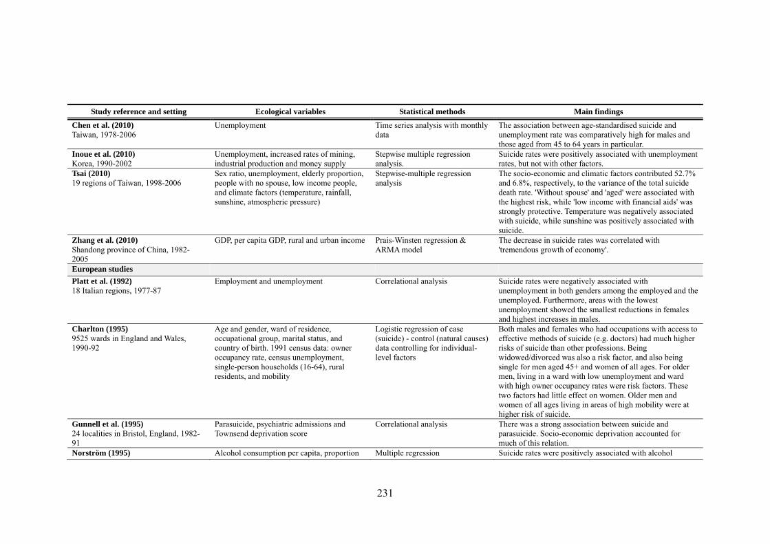
231

Study reference and setting Ecological variables Statistical methods Main findings

Chen et al. (2010) Taiwan, 1978-2006

Unemployment Time series analysis with monthly data

The association between age-standardised suicide and unemployment rate was comparatively high for males and those aged from 45 to 64 years in particular.

Inoue et al. (2010) Korea, 1990-2002

Unemployment, increased rates of mining, industrial production and money supply

Stepwise multiple regression analysis.

Suicide rates were positively associated with unemployment rates, but not with other factors.

Tsai (2010) 19 regions of Taiwan, 1998-2006

Sex ratio, unemployment, elderly proportion, people with no spouse, low income people, and climate factors (temperature, rainfall, sunshine, atmospheric pressure)

Stepwise-multiple regression analysis

The socio-economic and climatic factors contributed 52.7% and 6.8%, respectively, to the variance of the total suicide death rate. 'Without spouse' and 'aged' were associated with the highest risk, while 'low income with financial aids' was strongly protective. Temperature was negatively associated with suicide, while sunshine was positively associated with suicide.

Zhang et al. (2010) Shandong province of China, 1982-2005

GDP, per capita GDP, rural and urban income Prais-Winsten regression & ARMA model

The decrease in suicide rates was correlated with 'tremendous growth of economy'.

European studies

Platt et al. (1992) 18 Italian regions, 1977-87

Employment and unemployment Correlational analysis Suicide rates were negatively associated with unemployment in both genders among the employed and the unemployed. Furthermore, areas with the lowest unemployment showed the smallest reductions in females and highest increases in males.

Charlton (1995) 9525 wards in England and Wales, 1990-92

Age and gender, ward of residence, occupational group, marital status, and country of birth. 1991 census data: owner occupancy rate, census unemployment, single-person households (16-64), rural residents, and mobility

Logistic regression of case (suicide) - control (natural causes) data controlling for individual-level factors

Both males and females who had occupations with access to effective methods of suicide (e.g. doctors) had much higher risks of suicide than other professions. Being widowed/divorced was also a risk factor, and also being single for men aged 45+ and women of all ages. For older men, living in a ward with low unemployment and ward with high owner occupancy rates were risk factors. These two factors had little effect on women. Older men and women of all ages living in areas of high mobility were at higher risk of suicide.

Gunnell et al. (1995) 24 localities in Bristol, England, 1982-91

Parasuicide, psychiatric admissions and Townsend deprivation score

Correlational analysis There was a strong association between suicide and parasuicide. Socio-economic deprivation accounted for much of this relation.

Norström (1995) Alcohol consumption per capita, proportion Multiple regression Suicide rates were positively associated with alcohol

232

Study reference and setting Ecological variables Statistical methods Main findings

24 Swedish counties, 1963-65 divorced, religiosity index, unemployment and urbanisation

consumption and religiosity.

Congdon (1996a) 758 electoral wards in Greater London, 1990-92

Townsend deprivation index and social fragmentation score (termed ‘anomie score’) - combining levels of unmarried adults, single-person privately renting households and population turnover

Negative Binomial regression at borough level and non-parametric Poisson mixture model at ward level

A substantial variation in suicide rates across areas. Area deprivation was strongly associated with suicide rates.

Congdon (1996b) 758 electoral wards in Greater London, 1990-92

Psychiatric morbidity and 1991 census data for calculation of Townsend deprivation index and social fragmentation score - as described in Congdon (1996a)

Correlational analysis and non-parametric Poisson mixture - with varying intercepts and regression coefficients.

Male suicide rates were similarly associated with social fragmentation score and deprivation, while female suicide rates were more strongly associated with social fragmentation. Evidence for contextual effects of these associations according to geographical setting.

Ferrada-Noli (1996) 1 poorest and 1 richest county in Sweden, 1990

Comparison of suicide rates in the poorest and richest county

Descriptive analysis Higher suicide rates in the poorest county of Sweden and lower suicide rates in the richest county.

Saunderson and Langford (1996) Local Authority Districts, 1989-92

Unemployed population, single-person (below pensionable age) households, low social class, agricultural employment and Asian ethnic origin

Multiple regression Single-person households was the strongest predictor of both suicide and undetermined deaths in both genders, but stronger in females. In males, low social class and agricultural employment were better associated with suicide than undetermined deaths whereas the opposite was found for unemployment and Asian ethnicity.

Congdon (1997) 758 electoral wards in Greater London, 1990-92

1991 census data: Townsend deprivation index and social fragmentation score

Poisson regression with spatially structured and unstructured random effects fitted by MCMC methods in BUGS.

Male suicide was more strongly associated with deprivation than social fragmentation, but the opposite was observed for female.

Ferrada-Noli (1997c) 10 poorest and 10 richest municipalities of Sweden, 1990

Average income, older people in need of municipal social assistance, elderly living in municipality-managed service-homes

Chi-square test The relative frequency of suicide was 1.6 times greater for Swedes from the low-income municipalities than for those from the high-income ones. The group of municipalities with the highest suicide rate had a significantly higher proportion of older people in need of municipal social assistance at home and also a higher proportion of elderly living in municipality-managed 'service homes'.

Ferrada-Noli (1997b) 24 counties in Sweden, 1980

Average county income, county social care expenditure

Correlational analysis The counties with the highest suicide rates were found to have the highest percentage of people in the lowest income class and also the highest percentage of households

233

Study reference and setting Ecological variables Statistical methods Main findings

admitting social help.

Ferrada-Noli (1997a) Psychiatric catchment areas of the Karolinska Hospital in Stockholm, Sweden, 1990-1994.

Health indicators (life expectancy and early retirement) and socio-economic indicators (occupation intensity, dwellings by size of dwelling, home ownership, average income of the employed, public or municipal expenditure on education). Population density

Tabular and graphical analyses The area with a higher proportion of suicides had also a higher proportion of individuals who retired early, lower life expectancy at birth, higher unemployment, lower level of income, less public expenditure for education, less proportion of home ownership, and persons bound to one-room dwellings.

Marusic (1998) 60 communes in Slovenia, 1985-94

Depression, alcohol-related psychiatric morbidity, divorce and unemployment rates, average income per capita, criminal offence and homicide rates, Catholic/non-religious and hours of sunshine

Multiple linear regression and principal component analysis.

Higher suicide rate was most consistently associated with higher prevalence of alcohol psychosis (except for the youngest age group) and percentage Catholics (except for the oldest age group). No association was found for depression, unemployment and divorce.

Neeleman (1998) 11 provinces in the Netherlands, 1985-94

Nationwide survey indices of religiousness including church membership and attendance controlling for unemployment, education and rurality

Population weighted multiple regression rates

Suicide rate was negatively associated with levels of religiosity even after adjusting for socio-demographic variables. The association varied by age, with the weakest effect in the younger age-group.

Crawford and Prince (1999) 364 county districts in England, 1979-85 and 1986-92 (men aged 15-44 only)

1981 to 1991 changes in rates of single residents, being married, being unemployed, and people with no access to a car/van

One-Way Analysis of Variance and multiple linear regression

Areas with the lowest increase in suicide rates were those with the smallest rise in the proportion of people living alone, the greater increase in unemployment and highest levels of social deprivation.

Gunnell et al. (1999) England and Wales, 1921-1995

Unemployment Cochrane-Orcutt regression Unemployment was positively associated with suicide rates in both genders (15-44) and all ranges of males (15-24, 25-34, 35-44) and young females (15-24).

Hintikka et al. (1999) Finland, 1985-1995

Unemployment, GDP, divorce, mean alcohol consumption

Cochrane-Orcutt regression Suicide mortality in both genders increased during an economic upswing from 1985 to 1990, and decreased during an economic recession from 1990 to 1995. Suicide mortality was not associated with unemployment or divorce rates, but associated with mean alcohol consumption (male only).

Lester and Surault (1999) 95 French Departments, 1970

Marriage, divorce and birth rates Multiple linear regression Suicide rate was positively associated with marriage rates and negatively associated with divorce rates.

Neeleman and Wessely (1999) 109 electoral wards in South London, 1991-1993

Proportion of ethnic minorities adjusting for Jarman UPA score

Poisson regression with random effects

Minority suicide rates were higher in areas where minority groups were smaller even after adjusting for age, sex and deprivation.

Preti and Miotto (1999a) Social indicators including: marriage, Stepwise multiple regression. Suicide rate was positively associated with indicators of

234

Study reference and setting Ecological variables Statistical methods Main findings

20 Italian regions, 1992 separation and divorce rates and economic indicators including GDP per capita, employment and consumer rates as well as infant mortality, crime rates, social security and entertainment expenditure

wealth and social disintegration in both sexes, particularly for females. It was negatively associated with unemployment. Expenditure on welfare was the best predictor of suicide in both genders.

Preti and Miotto (1999b) Italy, 1982-1994

Employment and unemployment Correlational analysis Suicide rates among the unemployed were constantly higher than those among the employed, particularly for men.

Whitley et al. (1999) 633 parliamentary constituencies in Britain, 1981-92

Mean and change in Townsend deprivation score, social fragmentation score - as described in (Congdon, 1996a) - and abstention from voting based on 1981 and 1991 census

Population weighted multiple linear regression of suicide rates and change in suicide rates between 1981-1985 and 1986-1992

Suicide rate was more strongly associated with social fragmentation than deprivation.

Congdon (2000) 33 boroughs in London, 1979-94 in eight 2-year periods

1981 and 1991 census data for calculation of Townsend deprivation index and social fragmentation score - as described in Congdon (1996a)

Poisson regression with temporal and spatial (structured) random effects fitted by MCMC methods in BUGS

While associations with the social fragmentations were stronger than associations with deprivation, the effect of deprivation in explaining suicide variation seemed to be growing across time.

Rancans et al. (2001) Latvia, 1980-98

GDP, unemployment, first episode alcohol psychosis

Graphical analyses The sudden drop in GDP, the rapid increase in first-time alcohol psychosis and the percentage of people unemployed did not correspond strictly with the trend of suicide mortality.

Hawton et al. (2001) 103 electoral wards in Oxfordshire, 1985-95

Townsend deprivation index and social fragmentation score - as described above in Congdon (1996a)

Population weighted multiple linear regression

Suicide rate was most strongly associated with socio-economic deprivation, particularly in men. Association attenuated after adjusting for social fragmentation.

Smith et al. (2001) 633 parliamentary constituencies in the UK, 1981-92

Townsend deprivation index and social fragmentation score - as described above in Congdon (1996a)

Correlational analysis Social fragmentation was more strongly associated with suicide, while deprivation was more strongly associated with all- and other-cause mortality.

Bartlett et al. (2002) 95 Health Authorities in England, 1993-94

Mean and prevalence of elevated General Health Questionnaire (GHQ) and mean stress scores controlling for Jarman UPA socre

Weighted (by population or number of GHQ observations) multiple linear regression.

Deprivation was strongly associated with suicide, but not GHQ.

Gunnell et al. (2003) England and Wales, 1950-1998

Unemployment, divorce, motherhood, social fragmentation, female labour force participation, alcohol misuse, drug abuse, levels of religious belief/church attendance, levels of detection and treatment of mental illness, changes in availability/lethality of

Cochrane-Orcutt regression The factors most consistently associated with an increase in young male suicide were a rise in divorce, a decline in marriage, and an increase in income inequality. These changes had little effect on suicide in young females. In older people, declines in suicide were associated with increases in GDP, the size of female workforce, marriage

235

Study reference and setting Ecological variables Statistical methods Main findings

favoured methods of suicide and the prescribing antidepressants.

Middleton et al. (2003) 9264 electoral wards in England and Wales, 1981-83 and 1991-93 (15-44 years old)

Population density and population potential as rurality indicators adjusting for changes in social fragmentation score, Townsend deprivation and unemployment between two periods

Negative Binomial regression People living in areas remote from the main centres of population seemed to be at the great risk of suicide, particularly for females.

Evans et al. (2004) 34 electoral wards in Bristol, 1991-92

Social fragmentation score - as described in Congdon (1996a) - Townsend deprivation index and psychiatric admission rates

Negative Binomial regression An association between suicide and social fragmentation appeared to be independent of socio-economic deprivation or psychiatric admissions. Psychiatric admissions were more strongly related to levels of socio-economic deprivation.

Middleton et al. (2004) 9264 electoral wards in England and Wales, 1991-93

Social fragmentation score - as described in Congdon (1996a) - and Townsend deprivation index (aggregate scores and individual components) and other area characteristics including levels of cirrhosis mortality and population density

Negative Binomial regression Indicators of social fragmentation were most consistently associated with suicide and persisted even after adjusting for the other area characteristics. Associations were weaker in the older age-group.

Lucey et al. (2005) Ireland, 1968-2000

GDP, unemployment, female labour force participation rate, alcohol expenditure, marriage rate, percent births outside of marriage, and crime rate

Time-trend analyses Significant associations between suicide rates (total, male and female) and socio-economic variables, but they disappeared when the first-differenced data were used except for crime rates. Positive association between female suicide rates and crime rates.

Rezaeian et al. (2006) Local authorities and electoral wards of England, respectively, suicides in North West Government Office Region during 1996-98

Income and employment indices of deprivation

A hierarchical Poisson or negative binomial model

There was a positive association between suicide rates and level of deprivations at ward-level, but not at local authority level.

Rezaeian et al. (2007) London boroughs, 1996-1998 National Confidential Inquiry into Suicide and Homicide by People with Mental Illness

The hot spots index of deprivation Log-linear negative binomial regression model

The rate of suicide decreased with decreasing deprivation as indicated by the 'hot spots' index, particularly for males 30-49.

Barstad (2008) Norway, 1948-2004

Social integration variables (rates of unemployment, divorce, marriage, fertility, and separation), alcohol consumption (potential confounder), economic variables

Box-Jenkins approach to time-series analysis

Separation had a greater impact than divorce on suicide rates for both genders. Marriage and unemployment were negatively associated with male suicide rates. Both increasing alcohol consumption and fewer marriages were

236

Study reference and setting Ecological variables Statistical methods Main findings

(GNP per 1000 inhabitants, public/social assistance per 1000 inhabitants)

suggested to be the factors affecting the soaring suicide rate for young men since 1970

Altinanahtar and Halicioglu (2009) Turkey, 1974-2007

Per capita income, divorce rate, urbanisation, liquidation

Auto-Regressive Distributed Lag (ARDL) time series analysis

The urbanisation had the highest impact on suicides, followed by per capita real income and liquidation.

Magnusson and Makinen (2010) 290 municipalities in Sweden, average suicide rate during 2002-04.

Income, education, unemployment levels and divorce rates

OLS regression The overall and female suicide rates were negatively associated with income, while the effect on male suicide rates was not statistically significant.

North American studies

Hasselback et al. (1991) 261 Canadian census divisions, 1989-86

Rates for all causes of mortality, mortality rate from cirrhosis, homicide, 5-19 years old proportion, average family income, single parent families, unemployment, living in rural areas, over 15 with less than grade 9 education, divorced, separated, Catholics, no religious affiliation, native ancestry, ethnic origin, French as mother tongue, immigrated, blue collar workers, sex ratio, population density

Correlational analysis and stepwise multiple regression

Suicide rate was positively associated with all-cause mortality, proportion of no religious affiliation, Francophone, Native people and immigrants. It was inversely associated with unemployment, average family income, social mobility, young population and population density.

Lester (1991) 48 states in the US, 1980

37 variables factor analysed into levels of urbanisation/wealth, unemployment, Roman Catholicism and social disintegration

Factor analysis and correlational analysis in urban and rural areas separately

Social disintegration was most strongly associated with both urban and rural suicide rates. Rural suicides were also higher in more urbanised states.

Trovato (1992) 9 Canadian provinces, 1971 and 1981

Married females labour force participation controlling for divorce rates, no religious affiliation and unemployment

Multiple log-linear regression of sex-specific suicide counts controlling for age

Married female force participation was positively associated in 1971 but negatively associated with 1981 with suicide in both genders.

Lester (1995) 48 states in the US, 1959-61

Birth, marriage, divorce and unemployment rates, median age, family income, latitude and longitude, place of birth

Correlational analysis Social area characteristics were more strongly associated with suicide rates of people born out-of-state rather than those born in-state (i.e. the association was significant only for the subgroup of people migrating to the states from far away or from abroad).

Zimmerman (1995) 50 states in the US, 1960, 1970, 1980, 1985, 1990 and 1995

Public welfare spending controlling for sex ratio, racial composition, divorce rates, unemployment, population density and population change

Multiple linear regression in each period separately

Suicide rate was most strongly associated with divorce rate and negatively associated with public spending. It was not associated with unemployment.

Burr et al. (1997) 209 Standard Metropolitan Statistical

Female labour force participation controlling for divorce rate, single-person households,

Multiple linear regression Suicide rate was most strongly associated with divorce rate in both genders. It was negatively associated with female

237

Study reference and setting Ecological variables Statistical methods Main findings

Areas in the US, 1970 and 1980 population density, mobility, average family income, Catholic church membership

labour force participation after adjusting for other factors in both genders in 1980. It was not associated with unemployment.

Burr et al. (1999) US metropolitan areas in 1980, Black male suicides

Social integration/regulation (marital disruption/black female-headed households, church membership, socio-economic component), Racial inequality (occupation/income differentiation), Controls (black male population, urban population, region), Interaction (SES level and racial inequality)

Negative binomial regression for black male suicide counts

The risk of black male suicide was higher in areas where occupational and income inequalities between blacks and whites were greater. Positive associations between suicide rates and marital disruption and black female-headed households.

Lester (2001) 48 states in the US, 1990

Gross state product, population size and proportion urban, divorce rate, interstate migration and female labour force participation

Multiple linear regression Suicide rate was negatively associated with gross state product only in white males. Positive associations with suicide rates were found for sociological determinants, especially divorce, in all groups.

Baller and Richardson (2002) 3,060 counties in the US, 1989-91 and 83 French Departments 1872-76

Social integration measured as residential stability (born outside department in France, same address five years earlier in the US), marital stability (divorce rates) and religiosity, controlled for income, young age, fertility and population size in France and income, ethnicity, median age and population density in the US

Spatial lag/error models Suicide rate was negatively associated with social integration in both settings. Spatial lag model fitted better (except in western states). Suicide clustered geographically even after taking into account clustering of social integration factors, which they termed, ‘imitation effect’.

Kunce and Anderson (2002) 51 US states over 11 years, 1985-95

10 census variables including unemployment rates, median household income, divorce rates, living alone households, young population, Christian affiliation and ethnicity

Generalised least squares regression with fixed and random area and time effects

Other than single-person households, the other socio-economic variables were not associated with variation in suicide rates across states after controlling for latent area and time effects.

Zimmerman (2002) 50 states in the US, 1960, 1970, 1980, 1985, 1990 and 1995

Public welfare spending controlling for sex ratio, racial composition, divorce rates, unemployment, population density and population change

Multiple linear regression in each period separately

Suicide rate was most strongly associated with divorce rate and negatively associated with public spending. It was not associated with unemployment.

Minoiu and Andres (2008) US states, 1982-1997

Income, migration, unemployment, population density, mountain, divorce, GINI index, health expenditure, welfare expenditure, time

Fixed-effects model The share of health and welfare in total public spending were strong predictors of suicide rates. Suicide rates were higher in states with higher divorce rates, but average income level, income inequality and unemployment did not

238

Study reference and setting Ecological variables Statistical methods Main findings

have a robust impact on suicides.

Kubrin and Wadsworth (2009) US cities, 2000, young white and black males

Race-specific measures of percent male joblessness, median family income, percent poverty, residential mobility, racial segregation, percent single-female households with children under 18 years, people with 25+ and at least a high school education, firearm suicides (gun availability), and racial inequality (unemployment, joblessness, education, and poverty)

Principal factor analysis and negative binomial regression

For both young blacks and whites (males), disadvantage was most strongly associated with suicide rates. Cities with higher levels of poverty, joblessness, and female-headed households with children, and lower levels of high school graduates and median family income, had more young black and young white male suicides. When gun availability was added to the model, the association between disadvantage and black male suicide rates disappeared.

Australian studies

Morrell et al. (1993) Australia, 1907-1990

Unemployment Autoregressive integrated moving average (ARIMA) techniques

Female suicide rates were generally stable throughout the period, while male suicide rates showed sharp fluctuations with the peaks coinciding with times of high unemployment. The association between the two for 15-24 year old males was comparatively high for the period, 1966-1990.

Krupinski et al. (1994) 11 labour force regions in Victoria, Australia, 1983-89

Unemployment rates and urban-rural classification

Correlational analysis Male suicides were higher in rural areas. Unemployment rates were positively associated with male suicide rates only.

Burnley (1994) New South Wales, Australia and statistical local areas in Sydney, 1985-91

Occupation, marital status Correlational analysis Never-married and divorced male manual workers were particularly at risk of committing suicide. Never-married and divorced women had elevated suicide levels.

Burnley (1995) New South Wales, Australia and statistical local areas in Sydney, 1985-91

Occupation, marital status Correlational analysis ‘Not currently married male manual workers’ were particularly at risk.

Cantor et al. (1995) Small areas of Queensland in Australia, average suicide rates during 1990-1992

Socio-economic index for economic disadvantage (low income, low education, high unemployment), and economic resources (income and expenditure of families, rent and home ownership etc.)

Correlational analysis Suicide rates were positively correlated with socio-economic disadvantage, and negatively associated with the proportion of families on high income, who owned their homes and who had large houses. Suicide rates of people with 55+ were least influenced by these factors. For females, only the most disadvantaged areas had higher suicide rates.

239

Study reference and setting Ecological variables Statistical methods Main findings

Page et al. (2002) Australian local government areas, 1994-98

Three census-based indices of socio-economic status: Index of Relative socio-economic disadvantage average income and unemployment levels), Index of Economic Resources (income, home and vehicle ownership) and Index of Education and Occupation

Poisson regression adjusted for age, country of birth and rurality/ remoteness

Male suicide rates were positively associated with socio-economic disadvantage as measured by all three indicators. Female suicide rates were positively associated with economic resources but inversely with the index of education and occupation.

Qi et al. (2009) Small area of Queensland in Australia, average suicide rates during 1999-2003

Four indices: Index of Relative Socio-economic Advantage and Disadvantage, Index of Relative Socio-economic Disadvantage (i.e., low income, educational level, high unemployment, unskilled occupations), Index of Economic Resources (economic resources of residents and households), and Index of Education and Occupation. Indigenous population (%), unemployment, low income (%), low educational level (%), meteorological data (monthly rainfall, maximum temperature, minimum temperature)

Generalised estimating equation regression model with Poisson distribution, and semivariogram analysis for spatial regression

Maximum temperature, unemployment rate, the proportion of indigenous population and the proportion of population with low individual income were positively associated with suicides.

240

5.3. DATA AND METHODS

5.3.1. DATA

Suicide statistics (1980-2009) for Hong Kong, Japan and Singapore were taken

from the WHO mortality database which contains the number of deaths by

country, year, sex, age group, and cause of deaths (WHO, 2012). The data also

provide the population by country, year, sex and age group. While the WHO

mortality database included Korea, some years were missing. Consequently,

suicide statistics for 1983-2009 were taken from the Korean national statistics

online database (KOSIS), which provides suicide rates by five-year age groups.

The WHO mortality database does not include Taiwan. Both suicide and

population statistics for the years 1980-2009 were obtained directly from the

Department of Health of the Executive Yuan of Taiwan (2012).

The cause of death was coded in one of the four International Classification of

Disease (ICD) versions: ICD 7th, ICD 8th, ICD 9th, and ICD 10th versions.

Suicidal death was defined when the cause of death was coded as E963 or within

the range from E970 to E979 by the ICD 7th version, E950 to E959 by the ICD

8th or 9th versions, and X60 to X84 by the ICD 10th version.

Suicide rates, the number of suicide deaths per 100,000 population, were first

calculated for the following age groups in order to standardise the different age

structures across countries and over time: 15-20, 20-24, 25-29, 30-34, 35-39, 40-

44, 45-49, 50-54, 55-59, 60-64, 65-69, 70-74 and 75+. Age-standardised total

suicide rates were then derived through a direct standardisation method using the

241

WHO world standard population structure (see Table A5.1 in the Appendix),

which was based on the average world population structure for the period 2000-

2025 (Ahmad et al., 2001). Age-standardised suicide rates were also calculated

for males and females as well as specific age groups (15-24, 25-44, 45-64, and

65+).

Explanatory variables

In line with the theoretical frameworks of Hamermesh and Soss (1974), as well

as that of Durkheim (1897/2002), the present analysis focused on the impact of

economic change and social integration/fragmentation on suicide mortality. GDP

growth (International Monetary Fund, 2012) and unemployment rate

(International Monetary Fund, 2012) were employed as proxy indications of

economic change. Potential multicollinearity between GDP growth and

unemployment rate may, however, weaken their respective associations with

suicide rates. Rates of divorce, fertility and marriage, on the other hand, were

included as a proxy for social integration/fragmentation – an approach that is

commonly taken in the literature. The rates were obtained from the KOSIS

database for Korea (2012a), the Census and Statistics Department for Hong Kong

(2012), the Ministry of Health, Labour and Welfare (2011) (marriage and divorce

rates) and OECD Factbook 2010 (fertility rate) (OECD, 2010) for Japan, the

Singstat time series online data directory for Singapore (2011), and the DOH

Statistical Yearbook 2009 for Taiwan (2012). In order to account for the

differences in economic development between countries and across time, the

models also included a country-specific trend of per capita GDP, which was a

linear prediction of per capita GDP for each country (Heston et al., 2011).

242

The details of these variables are summarised in Table 5.4.

Table 5.4. Variables in the statistical models for suicide mortality

Definition Min Max Mean (SD)

Total Suicide rate Number of total suicides per 100,1000 population

8.9 35.3 17.2 (5.3)

Male suicide rate Number of male suicides per 100,1000 males

11.3 47.7 23.1 (8.3)

Female suicide rate Number of female suicides per 100,1000 females

5.7 24.7 11.7 (2.4)

Trend GDP Predicted trend of GDP per capita, based on GDP per capita at 2005 constant prices (PPP)

5801 47268 23617 (9066)

GDP growth Percent change in GDP, constant prices

-6.3 13.4 5.3 (4.0)

Unemployment Percent of the unemployed in total labour force

1.1 7.9 3.3 (1.4)

Divorce rate Number of divorce per 1000 population

0.4 3.5 1.6 (0.6)

Marriage rate Number of marriage per 1000 population

4.6 10.6 7.3 (1.3)

Fertility rate Number of children born to women aged 15-49

0.9 2.5 1.5 (0.3)

5.3.2. Econometric model

Panel data analysis

Panel data analysis was first carried out to investigate an association between

age-adjusted suicide rates and explanatory variables across five Asian countries

over the past 30 years (1980-2009). A fixed effects (FE) model was employed to

control for a fixed national culture of suicide and institutional practices that

might have influenced data collection. That is, the inclusion of FE, which is

conceptually identical to the inclusion of country dummy variables, adjusts for

the average differences across countries in any observable or unobservable

243

variables. The FE model thus relies on the variation within each country (i.e.

within-country variation), holding constant the average effects of each country

(i.e. between-country variation). An FE model can produce consistent estimates

even if the unobserved variables (or omitted factors) are correlated with the

regressors at the country level. A random effects (RE) model, on the other hand,

relies on both within- and between-country variation, and assumes that they are

not correlated. If this assumption holds, an FE model could be less efficient than

an RE model because the former loses degrees of freedom since an additional

number of (country) dummy variables are required. The Hausman test was

conducted to examine whether the coefficients estimated by the FE model

systematically differ from those by the RE model. If the test rejects the null

hypothesis, it indicates that failing to control for the country-specific FE would

provide biased estimates and thus the model should include the FE (Neumayer,

2003, pp.6). Otherwise, the results from both FE and RE models are likely to be

valid.

The statistical model specified below adopted the approach taken in a recent

European study that estimated the impact of unemployment on suicide mortality

(Stuckler et al., 2009):

tiii

k

jtjijti ettxS ,

1,, )(

(5.1)

where i is country and t is year, tiS , is the suicide rate at time t for country i, is

a constant term, tjix , is the value of regressor j (j=1,..,k), j is a parameter of

regressor j, is the average time trend of suicide rates, i is the country-specific

trend of suicide rates, i is the average country-fixed effects implicitly assumed

244

in the FE model, and ie denotes an error term. In the RE model, the country-

specific effects are assumed to be uncorrelated with the regressors, and thus can

be regarded as part of a composite error term tiiti e ,, .

The variables expressed in levels are, however, prone to generate spurious

relationships as they often exhibit a non-stationary property over time (ibid).

When the variables are trending, a regression of one on the other could produce a

high level of goodness of fit even if they are totally unrelated. Therefore, the

present analysis also examined an association between percentage changes in

suicide rates and the set of regressors13. Trend GDP, which is trend-stationary,

was nonetheless included as actual levels (instead of percentage change) to

control for differences in economic development across countries and over time.

This second model can be written formally as follows,

tiii

k

jtjijti ettxtrendGDPS ,

2,1, )(

(5.2)

Standard errors were also clustered by country to reflect the fact that countries

were not sampled independently and also to estimate unbiased standard errors in

the presence of serial correlation and heteroscedasticity across countries

(Stuckler et al., 2009). All analyses were repeated for age group-specific and

gender-specific suicide rates.

Time-series analysis

Country-specific time-series analyses were also carried out to complement the

13 Consistent with the study by Stuckler et al.(2009), unemployment and GDP growth were included as their first differences as they were already expressed in percentage.

245

panel data analyses and to address any country-specific associations between

suicide rates and the set of regressors. Cochrane-Orcutt estimation was employed

to adjust the linear model for serial correlation in the error term (Cochrane and

Orcutt, 1949).

The following model was first considered for each country, which is identical to

the panel data model above but without country and trend-specific terms:

t

k

jtjjt exS

1, (5.3)

The error term can be serially correlated over time as such that:

1||,1 ttt ee (5.4)

The Cochrane-Orcutt procedure then transforms the model as below,

ttj

k

jtjjtt xxSS

)()1( 1,

1,1 (5.5)

The model estimates the parameters at the minimum sum of squared residuals.

Country-specific time-series analyses were also conducted for percentage

changes in suicide rates and the set of regressors as follows,

ttj

k

jtjjtttt xxtrendGDPtrendGDPSS

)()()1( 1,

2,111

(5.6)

All analyses were repeated for age group-specific and gender-specific suicide

rates for each country.

Test for stationarity of variables

As explained above, the analysis considered variables in both levels and

246

percentage changes. However, if the variables contain stochastic trends, the

analyses are prone to produce spurious findings. Therefore, the presence of unit

root (i.e. non-stationary process) was tested for all variables (actual levels and

percentage change). The Dickey-Fuller (DF) test was employed for this purpose

on the time series data (i.e. each variable for each country) (Dickey and Fuller,

1979). Im, Pesaran, and Shin (2003) modified the DF test so that it (or the IPS

test) can be employed for the same purpose on the panel data. Of note, the IPS

test requires a balanced panel, and thus the test was implemented with the data

over the period 1983-2009 since suicide rates for Korea were available for 1983

onwards.

a. Dickey-fuller (DF) unit-root test

The DF test tests for a unit root in an autoregressive model (Dickey and Fuller,

1979). The following observation underlies the rationale of this test: (1) if a time-

series variable is stationary (or trend stationary), it has a tendency to return to a

constant (or deterministically trending) mean. This implies that large values will

tend to be followed by smaller values (negative changes) and small values will

tend to be followed by larger values (positive changes). The level of the series

will then be a significant predictor of next period’s change in the series, and that

will result in a negative coefficient; (2) On the other hand, if the series is

integrated (i.e. the presence of unit root), the current level of the series will not

have relevant information for predicting the next period’s change (e.g. random

walk).

This can formally be written as follows:

247

ttt eStS 1 (5.7)

where tS is the first difference in suicide rates at year=t (i.e. the change from

the previous year), is a constant term, is a deterministic time trend, 1tS is

the lagged level of suicide rates, is the coefficient of the lagged suicide rate,

and ie denotes an error term. The test is then carried out under the null

hypothesis that the variable contains a unit root (i.e. =0) against the alternative

hypothesis that the variable was generated by a stationary process, using the

following DF t-statistic:

)ˆ(

ˆ

SEt (5.8)

The present analysis tested the presence of a unit root in every variable (i.e., both

suicide rates and a set of regressors in both levels and percentage changes) with a

constant term only (i.e., drift) (i.e. =0). It was also tested with both drift and

deterministic time trend included.

b. Im, Pesaran and Shin (IPS) panel unit root tests

As one of the derivatives of the DF test, the IPS test can be used to test for the

presence of a unit root in a balanced panel (Im et al., 2003). It is also not as

restrictive as other types of panel unit root tests such as the Levin-Lin-Chu test

(Levin et al., 2002) since it allows for heterogeneous coefficients across panels.

The test first conducts separate (augmented) DF unit root tests for each panel as

follows:

titiiiiti eStS ,1,, (5.9)

248

It then assesses the null hypothesis of a unit-root in all cross-sectional series (i.e.

0i for all panels, i=1,…, N) against the alternative that at least one series is

stationary, using the DF t-statistics averaged across panels (

N

iit

Nt

1

1 ). If this

statistic is properly standardised, it asymptotically follows the standard normal

distribution.

As for the country-specific analyses, the presence of a unit root was tested for

every variable in a balanced panel (1983-2009) (i.e. both suicide rates and the set

of regressors in both levels and percentage changes) with a constant term only

(i.e. drift) (i.e. =0). It was also tested with both drift and deterministic time

trend included.

5.4. RESULTS

5.4.1. Visual inspection of suicide rates in five Asian countries

Figure 5.1 depicts the trend of age-adjusted overall suicide rates (per 100,000

population) over a 30-year period (1980-2009) in five Asian countries, Korea,

Hong Kong, Japan, Singapore and Taiwan. Korea exhibited the sharpest rise in

suicide rates amongst these countries. The rates, which started rising in the early

1990s, surpassed those of Japan in the early 2000s and have since remained the

highest in the region.

The trends of suicide rates were also charted by age groups within each gender

for further examination (Figure 5.2). Two observations were most apparent on

249

inspection. Relative to their counterparts in the other four Asian countries,

suicide rates in Korean females aged 25-44 years had an abrupt incline, doubling

from a rate of 12.3 in 2006 to 26.2 in 2009. This atypical trajectory was even

more outstanding for the Korean elderly. Amongst Korean men aged 65 and over,

suicide rates climbed steadily from being the lowest amongst their Asian

counterparts and deviated abruptly from the rest since the emergence of the

economic crisis in 1997/98, rising from a rate of 23.2 in 1983 to 66.8 in 1998,

eventually hitting 127.3 by 2009. A similar trajectory deviation was observed

amongst Korean women aged 65 and over, for whom suicide rates climbed from

8.5 in 1983 to 24.7 in 1998 and 50.0 by 2009. Across the four other Asian

countries, the average suicide rate in this group of elderly men actually fell from

56.7 (SD: 7.0) in 1980 to 38.6 (SD: 7.3) in 2009. Similarly, the average suicide

rate in this group of elderly women actually fell from 42.5 (SD: 9.2) in 1980 to

19.8 (SD: 2.3) in 2009.

Figure 5.1. Total suicide rates (per 100,000 population)

250

Figure 5.2. Suicide rates by gender and age groups

j. Female suicide rates (65+)

a. Male suicide rates (all age)

c. Male suicide rates (15-24) d. Female suicide rates (15-24)

e. Male suicide rates (25-44) f. Female suicide rates (25-44)

g. Male suicide rates (45-64) h. Female suicide rates (45-64)

i. Male suicide rates (65+)

b. Female suicide rates (all age)

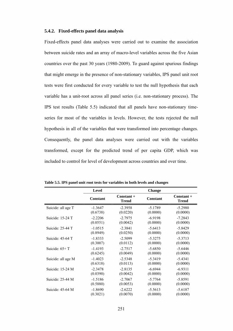
251

5.4.2. Fixed-effects panel data analysis

Fixed-effects panel data analyses were carried out to examine the association

between suicide rates and an array of macro-level variables across the five Asian

countries over the past 30 years (1980-2009). To guard against spurious findings

that might emerge in the presence of non-stationary variables, IPS panel unit root

tests were first conducted for every variable to test the null hypothesis that each

variable has a unit-root across all panel series (i.e. non-stationary process). The

IPS test results (Table 5.5) indicated that all panels have non-stationary time-

series for most of the variables in levels. However, the tests rejected the null

hypothesis in all of the variables that were transformed into percentage changes.

Consequently, the panel data analyses were carried out with the variables

transformed, except for the predicted trend of per capita GDP, which was

included to control for level of development across countries and over time.

Table 5.5. IPS panel unit root tests for variables in both levels and changes

Level Change

Constant Constant +

Trend Constant

Constant + Trend

Suicide: all age T -1.3647 (0.6738)

-2.3958 (0.0220)

-5.1789 (0.0000)

-5.2980 (0.0000)

Suicide: 15-24 T -2.2206 (0.0551)

-2.7975 (0.0042)

-6.9198 (0.0000)

-7.2843 (0.0000)

Suicide: 25-44 T -1.0515 (0.8949)

-2.3841 (0.0250)

-5.6413 (0.0000)

-5.8429 (0.0000)

Suicide: 45-64 T -1.8333 (0.3007)

-2.5099 (0.0112)

-5.3275 (0.0000)

-5.3713 (0.0000)

Suicide: 65+ T -1.4193 (0.6245)

-2.7517 (0.0049)

-5.6850 (0.0000)

-5.6446 (0.0000)

Suicide: all age M -1.4023 (0.6318)

-2.5348 (0.0113)

-5.3419 (0.0000)

-5.4341 (0.0000)

Suicide: 15-24 M -2.3478 (0.0390)

-2.8135 (0.0042)

-6.6944 (0.0000)

-6.9311 (0.0000)

Suicide: 25-44 M -1.5186 (0.5880)

-2.7067 (0.0053)

-5.7764 (0.0000)

-5.8591 (0.0000)

Suicide: 45-64 M -1.8690 (0.3021)

-2.6222 (0.0070)

-5.5613 (0.0000)

-5.6187 (0.0000)

252

Suicide: 65+ M -2.0386 (0.1622)

-2.9584 (0.0016)

-5.7178 (0.0000)

-5.7166 (0.0000)

Suicide: all age F -1.4932 (0.5969)

-2.2927 (0.0478)

-5.3777 (0.0000)

-5.5779 (0.0000)

Suicide: 15-24 F -2.8209 (0.0089)

-3.3867 (0.0002)

-7.3837 (0.0000)

-7.9883 (0.0000)

Suicide: 25-44 F -1.0014 (0.9318)

-2.1230 (0.1114)

-5.8337 (0.0000)

-6.3512 (0.0000)

Suicide: 45-64 F -1.9964 (0.2257)

-2.7477 (0.0040)

-5.5018 (0.0000)

-5.5717 (0.0000)

Suicide: 65+ F -1.1615 (0.8163)

-2.7731 (0.0047)

-5.8696 (0.0000)

-5.7806 (0.0000)

Trend per capita GDP†

0.0612 (1.0000)

- - -

Economic growth -2.9706 (0.0010)

-4.2996 (0.0000)

-6.6356 (0.0000)

-6.6042 (0.0000)

Unemployment -1.4219 (0.6325)

-1.9115 (0.1426)

-3.7650 (0.0000)

-3.8227 (0.0000)

Divorce rate -0.9870 (0.8965)

-1.7321 (0.3637)

-4.3491 (0.0000)

-4.6298 (0.0000)

Marriage rate -1.4719 (0.5192)

-2.4320 (0.0174)

-6.0804 (0.0000)

-6.0330 (0.0000)

Fertility rate -2.3372 (0.0370)

-2.2950 (0.0726)

-5.0931 (0.0000)

-5.3544 (0.0000)

Note: The values indicate t-bar statistics with p-values. It tests the null hypothesis of the existence of unit-root in all panels against the alternative that at least once series is stationary. †Trend per capita GDP is a predicted linear trend for per capita GDP. Its first differences are thus perfectly constant over time, disabling the tests with de-trending.

Panel data analyses investigated the association between changes in age-adjusted

suicide rates (as well as age group-specific suicide rates) and a set of macro-level

variables, holding constant the average effects of each country (i.e. fixed effects).

The results were presented for overall suicide rates (Table 5.6), male suicide rates

(Table 5.7) and female suicide rates (Table 5.8). The results of random-effects

models are also available in the Appendix (Table A5.2 – Table A5.4). Hausman

tests suggested no systematic differences between the two (see Table A5.2-Table

A5.4 in the Appendix). As the tests indicated, the fixed-effects estimation results

were largely similar to the random-effects estimation results. Of note, both

estimations provided low levels of R2, which is a typical problem when variables

are included in changes or first differences, rather than in levels (Stuckler et al.,

253

2009).

The fixed-effects (as well as the random-effects) results generally indicated a

negative association between suicide rates and economic growth. A 1% drop in

economic growth was associated with a 0.98% rise in age-adjusted overall

suicide rates (p=0.017). For men, the association with economic growth was

significant at the 5% level in age groups 25-44, 45-64 and 65+, while for women

the effect was significant in age group 15-24 only (significant in age group 25-44

at the 10% level). The random effects estimations, however, showed significant

associations across most age groups in both genders, except for males aged

between 15-24 (significant at the 10% level) and females aged 65+.

Table 5.6. Fixed-effect panel data analyses for change (%) in total suicide rates

Total 15-24 25-44 45-64 65+

Trend GDP -0.00

(0.00)** 0.00

(0.00)** -0.00

(0.00)*** 0.00 (0.00)

-0.00 (0.00)***

∆Economic growth -0.98

(0.25)** -1.31

(0.60)* -0.83

(0.19)** -0.82

(0.18)** -0.96

(0.39)*

∆Unemployment 2.30 (2.21) 1.42 (2.12) 1.72 (2.23) 4.66 (3.18) 0.48 (1.53)

∆Divorce 0.07 (0.15) -0.11 (0.15) 0.24 (0.14) 0.03 (0.21) 0.04 (0.15)

∆Marriage -0.13 (0.24) -0.26 (0.40) 0.13 (0.14) -0.20 (0.22) -0.24 (0.28)

∆Fertility -0.06 (0.21) 0.10 (0.44) -0.20 (0.27) -0.05 (0.10) -0.03 (0.29)

Country FE Yes Yes Yes Yes Yes

Country trends Yes Yes Yes Yes Yes

R2 0.1638 0.0813 0.1058 0.1512 0.1191

Asterisks indicate a statistical significance at 1% (***), 5% (**), and 10% (*). Note: year trend was dropped due to collinearity.

254

Table 5.7. Fixed-effects panel data analyses for change (%) in male suicide rates

Total 15-24 25-44 45-64 65+

Trend GDP -0.00

(0.00)** 0.00

(0.00)*** -0.00 (0.00) -0.00 (0.00)

-0.00 (0.00)***

∆Economic growth -1.02 (0.27) -1.69 (0.96) -0.91

(0.30)** -0.75

(0.15)*** -0.93

(0.30)**

∆Unemployment 3.71 (2.50) -0.83 (3.54) 2.80 (2.36) 6.75 (4.65) 1.98 (1.05)

∆Divorce 0.15 (0.14) 0.21 (0.10) 0.38 (0.15)* 0.10 (0.20) 0.04 (0.20)

∆Marriage -0.09 (0.24) 0.07 (0.48) 0.11 (0.25) -0.38 (0.36) -0.10 (0.18)

∆Fertility -0.01 (0.30) -0.49 (0.45) -0.01 (0.31) -0.21 (0.13) 0.20 (0.47)

Country FE Yes Yes Yes Yes Yes

Country trends Yes Yes Yes Yes Yes

R2 0.1713 0.1003 0.1344 0.1584 0.0754

Asterisks indicate a statistical significance at 1% (***), 5% (**), and 10% (*). Note: year trend was dropped due to collinearity.

Table 5.8. Fixed-effects panel data analyses for change (%) in female suicide rates

Total 15-24 25-44 45-64 65+

Trend GDP -0.00

(0.00)*** 0.00

(0.00)*** -0.00

(0.00)*** -0.00 (0.00) 0.00 (0.00)*

∆Economic growth -0.88

(0.23)** -1.06

(0.28)** -0.77

(0.31)* -0.88 (0.43) -0.93 (0.59)

∆Unemployment -0.20 (1.58) 2.80 (1.24)* -0.91 (2.27) 0.56 (1.78) -0.78 (1.66)

∆Divorce -0.08 (0.15) -0.54

(0.20)* -0.02 (0.12) -0.15 (0.39) 0.06 (0.22)

∆Marriage -0.18 (0.24) -0.75 (0.47) 0.12 (0.18) 0.21 (0.14) -0.36 (0.42)

∆Fertility -0.07 (0.09) 0.86 (0.65) -0.46 (0.29) 0.18 (0.22) -0.31 (0.20)

Country FE Yes Yes Yes Yes Yes

Country trends Yes Yes Yes Yes Yes

R2 0.1286 0.0715 0.0604 0.0443 0.0706

Asterisks indicate a statistical significance at 1% (***), 5% (**), and 10% (*). Note: year trend was dropped due to collinearity.

5.4.3. Results of country-specific analysis

In light of the atypical trend of suicide rates in Korea, time-series analysis was

also repeated for each country separately to complement earlier findings on the

influence of macro-level variables. The DF time-series unit root tests also

255

indicated the presence of non-stationary properties in most of the variables in

levels, but again rejected the null hypothesis of the non-stationarity in all of the

variables that were transformed into percentage changes, except for

unemployment rate in Japan (Table 5.9 for Korea; Table A5.5 – Table A5.8 in the

Appendix for the rest of the countries).

Table 5.9. DF time-series unit root tests for variables in both levels and changes: Korea

Level Change

Constant Constant +

Trend Constant

Constant + Trend

Suicide: all age T 0.406 (0.9817) -2.076 (0.5594) -4.772 (0.0001) -4.960 (0.0002)

Suicide: 15-24 T -1.619 (0.4731) -2.120 (0.5351) -6.732 (0.0000) -7.482 (0.0000)

Suicide: 25-44 T 0.255 (0.9752) -1.947 (0.6298) -5.487 (0.0000) -5.817 (0.0000)

Suicide: 45-64 T 0.012 (0.9595) -2.352 (0.4055) -4.634 (0.0001) -4.707 (0.0007)

Suicide: 65+ T 0.336 (0.9789) -1.745 (0.7306) -3.775 (0.0032) -3.722 (0.0210)

Suicide: all age M -0.047 (0.9544) -2.309 (0.4290) -4.622 (0.0001) -4.706 (0.0007)

Suicide: 15-24 M -2.657 (0.0818) -2.083 (0.5553) -5.386 (0.0000) -5.808 (0.0000)

Suicide: 25-44 M -0.687 (0.8502) -2.609 (0.2758) -5.086 (0.0000) -5.153 (0.0001)

Suicide: 45-64 M -0.306 (0.9246) -2.508 (0.3242) -4.941 (0.0000) -4.996 (0.0002)

Suicide: 65+ M 0.141 (0.9687) -1.795 (0.7070) -3.644 (0.0050) -3.577 (0.0319)

Suicide: all age F 1.145 (0.9956) -1.388 (0.864) -5.478 (0.0000) -6.003 (0.0000)

Suicide: 15-24 F -0.836 (0.8082) -2.625 (0.2686) -8.190 (0.0000) -9.143 (0.0000)

Suicide: 25-44 F 1.340 (0.9968) -0.632 (0.9773) -6.324 (0.0000) -7.399 (0.0000)

Suicide: 45-64 F 0.812 (0.9918) -1.740 (0.7328) -4.636 (0.0001) -4.715 (0.0007)

Suicide: 65+ F 0.279 (0.9764) -1.794 (0.7078) -4.683 (0.0001) -4.599 (0.0010)

Trend per capita GDP -0.063 (0.9530) - - -

Economic growth -4.221 (0.0006) -6.078 (0.0000) -8.025 (0.0000) -8.005 (0.0000)

Unemployment -2.669 (0.0795) -2.607 (0.2769) -4.510 (0.0002) -4.443 (0.0019)

Divorce rate -1.020 (0.7459) -1.209 (0.9086) -4.268 (0.0005) -4.649 (0.0009)

Marriage rate -1.080 (0.7229) -1.899 (0.6554) -4.681 (0.0001) -4.617 (0.0010)

Fertility rate -4.638 (0.0001) -3.763 (0.0185) -3.616 (0.0055) -3.688 (0.0232)

Note: The values indicate DF t-statistics with p-values. It tests the null hypothesis of the existence of unit-root against the alternative hypothesis that the variable was generated by a stationary process. †Trend per capita GDP is a predicted linear trend for per capita GDP. Its first difference is thus perfectly constant over time, disabling the tests with de-trending.

The results of time-series analyses for age-adjusted suicide rates as well as age

group-specific suicide rates (total, males and females) in Korea are presented in

Table 5.10 – 5.12 (see Tables A5.9 – Table A5.12 in the Appendix for the results

256

for other countries). In general, a change in divorce rates was most consistently

associated with a change in suicide rates across age groups and genders, except

for the trend GDP that was included to control for level of development.

Specifically, a 1% increase in divorce rates was associated with a 0.64% rise in

total suicide rates (p=0.025). The effect was greater for people aged 65 and over.

It was associated with a 0.90% increase in males (p=0.012) and a 0.86% in

females (p=0.022) who were aged 65 and over. The impact of divorce was,

however, observed only in limited age groups in other countries, mostly working

age groups (25-44 and 45-64) in Japan and Taiwan.

For Korea, the effect of economic growth was significant only at a 10% level in

working age males (25-44 and 45-64). More specifically, a 1% decline in GDP

growth was associated with a 1.11% rise in suicide rates in males aged between

45-64 years old (p=0.056). The effect of unemployment was also significant only

for this group (45-64) – every 1% increase in unemployment was associated with

a 6.85% rise in suicide rates (p=0.019). The impact of unemployment was also

noted for this group only in Hong Kong (at a 5% level) and Taiwan (at a 10%

level).

Change in marriage rates generally had a positive association with suicide rates

in age groups 15-24 and 65+. More specifically, a 1% rise in marriage rates was

associated with a 1.19% rise in suicide rates in males (p=0.096) and a 2.40% rise

in females (p=0.002) aged between 15-24 years old. It was also associated with a

1.01% rise in elderly males (+65) (p=0.096). A similar relationship was also

observed for Taiwanese males in 25-44 years old.

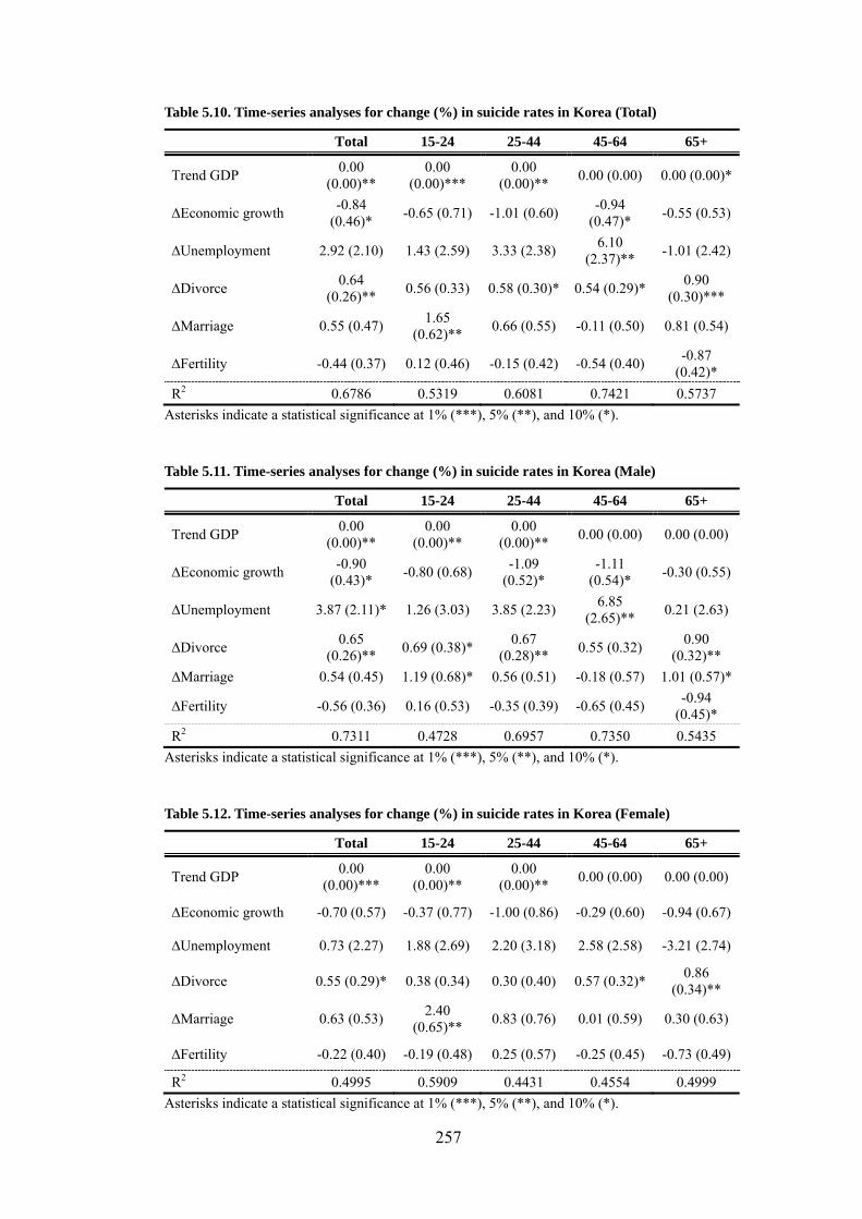
257

Table 5.10. Time-series analyses for change (%) in suicide rates in Korea (Total)

Total 15-24 25-44 45-64 65+

Trend GDP 0.00

(0.00)** 0.00

(0.00)*** 0.00

(0.00)** 0.00 (0.00) 0.00 (0.00)*

∆Economic growth -0.84

(0.46)* -0.65 (0.71) -1.01 (0.60)

-0.94 (0.47)*

-0.55 (0.53)

∆Unemployment 2.92 (2.10) 1.43 (2.59) 3.33 (2.38) 6.10

(2.37)** -1.01 (2.42)

∆Divorce 0.64

(0.26)** 0.56 (0.33) 0.58 (0.30)* 0.54 (0.29)*

0.90 (0.30)***

∆Marriage 0.55 (0.47) 1.65

(0.62)** 0.66 (0.55) -0.11 (0.50) 0.81 (0.54)

∆Fertility -0.44 (0.37) 0.12 (0.46) -0.15 (0.42) -0.54 (0.40) -0.87

(0.42)*

R2 0.6786 0.5319 0.6081 0.7421 0.5737

Asterisks indicate a statistical significance at 1% (***), 5% (**), and 10% (*).

Table 5.11. Time-series analyses for change (%) in suicide rates in Korea (Male)

Total 15-24 25-44 45-64 65+

Trend GDP 0.00

(0.00)** 0.00

(0.00)** 0.00

(0.00)** 0.00 (0.00) 0.00 (0.00)

∆Economic growth -0.90

(0.43)* -0.80 (0.68)

-1.09 (0.52)*

-1.11 (0.54)*

-0.30 (0.55)

∆Unemployment 3.87 (2.11)* 1.26 (3.03) 3.85 (2.23) 6.85

(2.65)** 0.21 (2.63)

∆Divorce 0.65

(0.26)** 0.69 (0.38)*

0.67 (0.28)**

0.55 (0.32) 0.90

(0.32)**

∆Marriage 0.54 (0.45) 1.19 (0.68)* 0.56 (0.51) -0.18 (0.57) 1.01 (0.57)*

∆Fertility -0.56 (0.36) 0.16 (0.53) -0.35 (0.39) -0.65 (0.45) -0.94

(0.45)*

R2 0.7311 0.4728 0.6957 0.7350 0.5435

Asterisks indicate a statistical significance at 1% (***), 5% (**), and 10% (*).

Table 5.12. Time-series analyses for change (%) in suicide rates in Korea (Female)

Total 15-24 25-44 45-64 65+

Trend GDP 0.00

(0.00)*** 0.00

(0.00)** 0.00

(0.00)** 0.00 (0.00) 0.00 (0.00)

∆Economic growth -0.70 (0.57) -0.37 (0.77) -1.00 (0.86) -0.29 (0.60) -0.94 (0.67)

∆Unemployment 0.73 (2.27) 1.88 (2.69) 2.20 (3.18) 2.58 (2.58) -3.21 (2.74)

∆Divorce 0.55 (0.29)* 0.38 (0.34) 0.30 (0.40) 0.57 (0.32)* 0.86

(0.34)**

∆Marriage 0.63 (0.53) 2.40

(0.65)** 0.83 (0.76) 0.01 (0.59) 0.30 (0.63)

∆Fertility -0.22 (0.40) -0.19 (0.48) 0.25 (0.57) -0.25 (0.45) -0.73 (0.49)

R2 0.4995 0.5909 0.4431 0.4554 0.4999

Asterisks indicate a statistical significance at 1% (***), 5% (**), and 10% (*).

258

5.5. DISCUSSION

The present analysis has brought to light a sharp increase in suicide rates in

Korea that is different from the experience over the same period in Hong Kong,

Japan, Singapore, and Taiwan - countries which are closely related in terms of

geography as well as culture. This atypical trend was most apparent for people

aged 65 and over, with suicide rates amongst Korean elderly men climbing from

23.2 in 1983 to 127.3 in 2009. Amongst Korean elderly women, suicide rates

increased from 8.5 to 50.0 over the same period. This trend is particularly

disturbing in light of the relatively stable or gradually declining suicide rates that

have been observed in other Asian countries. The analyses based on three

decades (1980-2009) of panel data from the five Asian countries generally point

to a link between economic growth and suicide rates. Specifically, a 1% drop in

GDP growth is associated with a 0.98% rise in age-adjusted overall suicide rates.

Country-specific time series analyses that were conducted for Korea further

suggest that low levels of social integration, as indicated by rising divorce rates,

may also have a role in rising suicide rates.

5.5.1. Suicide amongst the elderly in contemporary Korea

According to the economic theory of suicide suggested by Hamermesh and Soss

(1974), the suicide rate rises with age because ageing is associated with a

decrease in level of utility, driven by multiple losses such as health, status,

income, autonomy, roles and relations (Waern et al., 2003). This hypothesis is

fairly in line with what have been actually seen in most of industrialised

countries (Shah and De, 1998; Gunnell et al., 2003; Yip, 2008). However, a

259

recent cross-national study involving 54 countries found that suicide rates have

been declining amongst older people over the past decade (Shah et al., 2008),

implying a weakening link between ageing and disutility, plausibly due to an

improvement in the quality of life of older people in the most recent decade.

Evidence for a link between ageing and disutility is similarly lacking in the

present analysis for the Asian countries, with the exception of Korea.

The atypical trend in Korea implies that some aspects of modern Korean society

continue to strengthen and/or maintain the association between ageing and

disutility. The country-specific time-series analysis for Korea showed a relatively

consistent association between divorce and suicide rates across different age

groups – this finding was again unique to Korea. The association was the

strongest for people aged 65 and over. Specifically, a 1% increase in divorce

rates was associated with a 0.90% increase in suicide rates in elderly men, and a

0.86% increase in elderly women. In contrast, the association with divorce rates

was observed only for a few age groups in the other Asian countries, mostly

amongst working age groups (aged 25-44 and 45-64) in Japan and Taiwan. While

the ecological nature of the present analysis did not permit a straightforward

interpretation of the link between divorce and suicide rates, the former has been

commonly employed in the literature as an indication of the level of social

integration/fragmentation. With this caveat, the present findings support the

hypothesis that declining social integration (or increasing social fragmentation)

may be one of the driving forces for rising suicide rates in Korea, particularly

amongst the elderly. While experiencing social isolation and loss is not

uncommon in old age, these negative life events may be more debilitating in a

260

society where the climate of weakening social integration/fragmentation is no

longer able to sustain the family and social support networks that would have

buffered the elderly in the past. Furthermore, without sufficient social protection

policies, the elderly in Korea may also have less of a safety net against relative

and absolute poverty in the first place.

In Asia, elderly people have traditionally been cared for by their children within

the extended family. Such family support in Korea has greatly weakened as the

proportion of elderly people living with their children has declined from over

80% in 1981 to 29% by 2008 (OECD, 2011b). This figure includes elderly

people living with unmarried children, who may still require financial support

from their parents. Consistent with this trend, the proportion of Korean elderly

people living alone rose from 8.9% in 1990 to 32% in 2005 (The Ministry of

Health and Welfare, 2009). Such a transition from family-based care to a model

of social care for the elderly in Korea has left a substantial number facing

financial hardship amidst its unbalanced pace of development. This is reflected in

public spending for old-age benefits which stood at 1.7% of the 2007 GDP in

Korea, just a quarter of the OECD average (OECD, 2011b). With the National

Pension Scheme (NPS) introduced only in 1988, most pensioners still receive

partial pensions. In 2005, more than 45% of people aged 65 and over were thus

in relative poverty with incomes below one-half of median household income,

the highest proportion amongst OECD countries (ibid). Even though the Korean

government introduced two major programmes (the Basic Old-age Pension

system and Long Term Care Insurance) in 2008 in a response to the growing

elderly population, the benefits are still very limited compared to other OECD

261

countries.

Compounding such economic strain on the elderly in Korea is the social stigma

associated with being cared for in nursing home or long-term care facilities. This

prospect is perceived as disgraceful abandonment by the family and often as a

final resort in face of financial hardship and medical problems. A recent study

showed that the overall proportion of Korean elderly with clinically significant

depressive symptoms was 37.5% (Shin et al., 2012), and that the prevalence of

depression is expected to be greater in people living in such facilities (Jeong,

2005). Policy efforts aimed at strengthening the social safety net for the elderly

in Korea would need to tackle such societal attitudes to have any chance of being

effective.

5.5.2. Economic growth, unemployment and suicide rates

The present analysis also sheds light on the differential associations between

social changes and suicide rates at various stages over a person’s life course. In

particular, the associations between suicide rates and unemployment and

economic growth were most salient amongst middle-aged men in Korea. A 1%

increase in unemployment was associated with a 6.85% rise in suicide rates

amongst males between 45-64 years old. Similarly, a 1% decrease in economic

growth was associated with a 1.11% rise in suicide rates in this group although it

was significant only at a 10% level (p=0.056). These associations suggest that the

segment of the Korean population that is most susceptible to the negative impact

of economic downturn is middle-aged men. A similar pattern was also observed

for Hong Kong and Taiwan. While a 1% increase in unemployment was

262

associated with a 10.17% for this group in Japan, it did not reach statistical

significance.

Notably, while these findings are consistent with previous studies from Taiwan

(Chan et al., 2007; Chen et al., 2010) and Japan (Yamasaki et al., 2005), studies

from Australia (Morrell et al., 1993) and New Zealand (Blakely et al., 2003)

reported stronger associations between unemployment and suicide rates amongst

younger males (15-24/18-24 years old). This disparity in age group may in part

reflect socio-cultural differences between Asian and Western societies. In Asian

countries like Korea, it is common for young people to depend on their parents

until they have securely established a career (Chen et al., 2010). Such societal

norms mean that the financial burden of the family is much more likely to fall on

the middle-aged male members. The burden could be even more severe in

countries like Korea, where financial support for the unemployed is relatively

limited (OECD, 2011c). Although employment insurance, which was introduced

in 1995, provides unemployment benefits and opportunities of job trainings,

around 40% of employees are not registered for employment insurance in Korea

and thus not eligible for such benefits (Kim, 2010). Considering that employment

losses are often concentrated on unskilled workers who are likely to have no

employment insurance cover (OECD, 2011a), unskilled middle-aged male

workers potentially constitute the group that is most at-risk of both financial

strain and associated psychological distress in event of employment loss in Korea.

The burden of unemployment could also be compounded by an intimate link

between occupational status and people’s sense of identity and self-worth,

263

thereby further exacerbating the psychological distress in the case of such events

(Jahoda, 1981; Anderson et al., 2007). In the aftermath of the economic crisis in

1997/98, it was not uncommon for middle-aged men to keep news of their

employment loss undisclosed even to their families, preferring instead to

commute as usual and spend their time in other places such as parks or on trains

(Watts, 1998). Such reports reflect the non-trivial social and psychological

impact of the economic crisis/unemployment on middle-aged men in Korean

society. In face of such firmly entrenched societal norms and perceptions, policy

efforts aimed at ameliorating the economic adversity faced by middle-aged men

may also need to target interventions at the employment culture. A majority of

Korean firms set their mandatory retirement age at below 60 as recommended by

law. This means that the average employment tenure in Korea peaks at the age of

45-49, compared to the later age of 55-64 in most other OECD countries (OECD,

2011b). The enforcement of such an early retirement age, motivated in part to

minimize the costs incurred by the culture of seniority-based wages, leaves many

middle-aged and older workers in low-paid jobs, as they lack the productivity

and skills to cope with the rapidly changing needs of industry. Economic reforms

may require policy attention in the domain of employment laws, together with

stronger social protection and expanded social safety net for the unemployed.

5.5.3. Limitations

Several limitations should be noted in the present analysis when assessing the

policy implications. Firstly, this analysis relied on aggregate-level population

data, and thus the findings cannot be directly translated into interpretations about

individuals within the population. Secondly, while divorce rate is often employed

264

in the literature as a proxy for the level of social integration/fragmentation in a

given society, it is potentially problematic as revealed by the present analysis in

which marriage rates, a conceptually similar indicator, had a counter-intuitive

association with suicide rates. Thirdly while the present analysis considered key

indicators of socio-economic changes, the scope of explanation remains limited

in light of the complex and multifactorial causes of suicide (Gunnell et al., 2003).

Finally, the reliability of suicide statistics is likely to differ across countries.

However, as the present study focused on the changes in suicide rates within

each country, reliability differences between countries are not likely to pose a

major concern for the present analyses. Nonetheless, changes in levels of

reporting of suicide could have affected the temporal trends of suicide rates. For

instance, the social stigma toward suicide could have been more severe in the

past, possibly leading to a higher level of under-reporting (Lee et al., 2009). The

temporal trends of suicide rates thus could in part be explained by an

improvement in levels of reporting, although it is not clear whether changes in

levels of reporting would systematically differ by country.

5.6. CONCLUSIONS AND POLICY IMPLICATIONS

The present findings indicate that the phenomenon of rising suicide rates,

particularly amongst the elderly, is unique to Korea, and that the suicide

epidemic in contemporary Korea has social origins as argued by Durkheim.

Different age groups within the population are likely to require policy

interventions that target culturally-relevant attitudes and/or economic practices.

For the elderly in Korea, there is a need to strengthen methods of assisting family

support as well as formulating models of social care that are financially-

265

sustainable and culturally-sensitive. For middle-aged men in Korea, reforming

nationwide employment practices with regard to skills, training and retirement

may afford substantial social protection for them as well as those who depend on

them. In addition, increasing vigilance in a form of employment-related risk

assessment may provide valuable leads for timely intervention. The need for

further empirical research in this field remains ever more urgent in light of the

current economic climate worldwide.

266

CHAPTER 6: POLICY IMPLICATIONS AND CONCLUSIONS

Tackling persistent health inequalities between socio-economic groups has

surfaced prominently in the policy agenda worldwide. Korea is no exception. The

‘New Health Plan 2010’, established in 2005, aims to reduce health inequality

and ultimately improve overall quality of life of the nation. In Korea, the issue of

health inequality has steadily gained attention with widening income inequality

and increasing social polarisation following the economic crisis in the late 1990s.

However, this issue has remained poorly understood in the domain of mental

health, despite rapidly rising suicide rates and depression over the past decade in

Korea. As a first step, the thesis set out to provide a comprehensive overview and

analysis of health inequality in the domain of mental health, particularly for

depression and suicidal behaviour, in contemporary Korea.

The key findings or issues that emerged from the literature review and empirical

analyses are discussed here under the following headings:

• Summary of empirical findings and literature review

• Study limitations

• Implications for policy and further research

• Concluding remarks

6.1. SUMMARY OF EMPIRICAL FINDINGS

6.1.1. Income-related inequalities in mental health (Chapter 2)

This thesis first examined the trend of income-related inequalities in depression,

suicidal ideation and suicide attempts over a 10-year period (1998-2007)

267

following the country’s major economic crisis in 1997/98, using four waves of

the nationally representative household survey data. The concentration index (CI)

approach was employed to quantify the extent of income-related inequalities.

These were then decomposed to reveal the respective contributions of socio-

economic determinants.

The analyses revealed the existence of persistent pro-rich inequalities in the

prevalence of depression, suicidal ideation and suicide attempts over the 10-year

period following the economic crisis (i.e. poorer groups are doing worse). The

magnitude of the CIs was found to have doubled in all three instances, although

they exhibited different trends over this period. For depression, inequality

increased sharply between 1998 (CI: -0.126) and 2001 (CI: -0.278), and

remained relatively stable thereafter. Similarly, inequality in the prevalence of

suicidal ideation increased over time, but at a more gradual rate. In the case of

suicide attempts, inequality actually decreased between 1998 (CI: -0.221) and

2001 (CI: -0.175), but surged between 2005 (CI: -0.179) and 2007 (CI: -0.400).

The contrasting inequality trends for depression and suicide attempts over 1998-

2001 may in part be explained by a different time-lag impact of the economic

crisis. Amidst massive restructuring and tight austerity measures brought forth by

the IMF intervention, there was a rapid rise in both the unemployment rate and

income inequality in 1998. The social turmoil, which would have

disproportionately affected less privileged segments of the population, coincided

with a surge in suicide rates from 13.1 per 100,000 in 1997 to 18.4 in 1998

(KOSIS, 2012b). The higher level of income-related inequality in the prevalence

268

of suicide attempts in 1998, compared to 2001, may be a reflection of an acute

and potent impact of the economic crisis. The onset of depression, on the other

hand, is likely to involve a chronic course of symptoms prior to clinical diagnosis,

which is itself associated with considerable variation in the time since onset. The

rise in income-related inequality for depression from 1998 to 2001, in contrast to

the decline in inequality for suicide attempts, may therefore be a reflection of a

different time lag effect of the economic crisis on depression and suicide

attempts.

Despite these initial observations, a longer time perspective (1998-2007) has

revealed that pro-rich inequalities have doubled over the ten years since the

economic crisis, with an increasingly prominent income-gradient across all three

health outcomes, suicide attempts in particular. In addition, the CIs in the present

analysis indicate that the magnitude of inequality might be greater in mental

health than for general health. Based on the same data set as the one analysed in

this thesis, Shin and Kim (2007) reported CIs of -0.0116 for 1998, -0.0179 for

2001 and -0.0278 for 2005 in their assessment of income-related inequality in

self-reported general health. While their study also showed pro-rich inequality in

general health, the magnitudes were notably smaller than those found in the

present analyses.

The total inequalities (CIs) in the prevalence of depression and suicidal

behaviour were also decomposed into the contributions of other determinants.

The analysis generally indicated that income made the greatest contribution

toward inequality in all three health outcomes, followed by educational

269

attainment and employment status, although the magnitude of their respective

contributions varied across the years and the outcomes. In particular, the gross

contribution of income in the CI for suicide attempt in 2007 (-0.415) was

outstanding, with a strong effect on its prevalence (elasticity: -4.388).

6.1.2. Relationship between regional level income inequality and mental

health (Chapter 3)

Having elucidated the extent and trend of income-related inequality in population

mental health in Korea over the decade following the economic crisis, the next

empirical investigation of the thesis set out to examine whether income

inequality has a detrimental effect on population health, independent of a

person’s absolute level of income in Korea. Three theoretical frameworks have

been predominant in the literature for explaining the mechanisms underlying the

link between income inequality and health: (1) psychological distresses from

social comparison; (2) erosion of social capital; and (3) underinvestment in social

infrastructure (the neo-material interpretation). Much of the evidence supporting

these hypotheses has been based on cross-national or US studies. While the link

between income inequality and population health has been less well-established

in other countries, some recent evidence has emerged from studies in Asian

countries, notably Japan and China (Pei and Rodriguez, 2006; Kondo et al.,

2008; Ichida et al., 2009; Oshio and Kobayashi, 2009; 2010). In contributing

empirical findings from the Korean context, the present study is also a timely

investigation of an issue that is in urgent need of policy attention.

The second empirical investigation examined the relationship between regional-

270

level income inequality and mental health, using 2005 nationally representative

survey data. The outcomes included HRQoL, suicidal ideation and stress as

surrogate indicators of mental health. The association with (self-rated) general

health was also examined for comparative purposes. The Gini coefficient was

employed to measure regional-level income inequality. As the Gini coefficient

cannot differentiate between types of income distribution, the Generalised

Entropy (GE) indices with different sensitivity parameters were also employed to

check the robustness of the results. A series of regressions with different levels of

adjustments and outcomes were carried out but at a single level, rather than

multi-levels, because the survey structure of the KHANES could not be

appropriately taken into account by current multi-level modelling techniques.

The findings set out in Chapter 3 suggest that regional- level income inequality is

not an important determinant of population health in Korea. Instead, the variation

in health across regions may be largely attributable to the composition of

residents’ individual-level socio-economic and demographic characteristics. For

instance, although income inequality was correlated with HRQoL and self-rated

poor health at regional level, the associations disappeared once the analysis

adjusted for demographic characteristics. Despite the importance of

‘psychological stresses’ as a possible mechanism underlying the relation between

income inequality and health, suicidal ideation and psychological stress were not

correlated with regional-level income inequality, even before the adjustment for

individual-level factors.

The findings reveal that the absolute level of a person’s income is one of the key

271

determinants of individual health in Korea. In addition, level of health was also

found to be associated with other demographic and socio-economic factors. In

general, being female, being older, having a disturbed marriage, living in a

metropolitan area, having a lower level of educational attainment, and not having

regular full-time employment (e.g. unemployment) were associated with poorer

health outcomes. Of note, non-regular employment exhibited an equally strong

association as unemployment in the case of suicidal ideation. An exception was,

however, found for stress – a higher level of stress was associated with being

younger and having regular full-time employment. Somewhat notable was also

the observation that most of the associations between health and individual-level

factors (particularly age) attenuated once the analysis adjusted for underlying

health status (i.e. “objective poor health”) in the sensitivity analyses, implying

that medical conditions play a substantial role in population mental health (e.g.

suicidal ideation).

6.1.3. Geographical variation in suicide rates and area deprivation

(Chapter 4)

This thesis has also paid special attention to suicidal mortality in Korea in face of

the rapidly rising suicide rates and substantial variation in the rates observed

across regions within the country (Chapters 4 and 5). In light of the variation in

regional economic development within Korea, examining the geographical

distribution of suicide rates may also help to shed light on the link between

socio-economic inequality and population mental health.

Chapter 4 hence focused on the spatial patterning of age-standardised suicide

272

rates across small areas (district level) in Korea and the relationship between the

geographical distribution of age-standardised suicide rates and area deprivation,

using 2005 population census data and 2004-2006 mortality data. The

relationship was examined using a spatial lag model, since there was evidence of

spatial autocorrelation in the distribution of suicide rates across 250 districts of

Korea. In addition, the model included other area-level explanatory variables,

such as proportion of welfare budget, population density, and rates of divorce,

fertility and marriage. The present analysis adapted the index of area deprivation

available in a recent government report, which modified existing deprivation

indices such as the Townsend or the Carstairs Index to better reflect the Korean

context (Shin et al., 2009).

The present findings elucidated the spatial patterns of age-standardised suicide

rates in Korea, highlighting substantial geographical variations across districts.

The spatial mapping showed the concentration of high suicide rates in non-

metropolitan/rural areas in Korea such as Gangwon-do and Chungcheongnam-do.

The results of the spatial lag model suggested that area deprivation may have an

important role in shaping the geographical distribution of suicide in

contemporary Korea, particularly for male suicide rates. Compared to the least

deprived areas (1st quintile), there were about 12-13 more male suicide cases (per

100,000 males) in highly deprived areas (4th and 5th quintiles). Considering the

fact that the average OECD suicide rate in 2005 was approximately 12 per

100,000 population (OECD, 2011d), the impact of area deprivation on suicide in

Korea deserves policy attention.

273

In addition to area deprivation, population density, which was employed as a

proxy measure of the rurality of an area, also showed a positive association with

suicide rates. While material deprivation of rural areas (i.e. the lack of material

and infrastructural resources at both individual and area levels) was likely to be

accounted for by the level of area deprivation, the ecological association between

population density and suicide rates, independent of area deprivation, draws

attention to the potential influence of other aspects of rurality. These aspects may

include social isolation (or limited social networks) and the stigma associated

with mental health problems, as they are more likely to be severe in rural areas.

The present analysis also found an association between suicide rates and divorce

and fertility rates. Suicide rates were negatively associated with fertility rates and

positively associated with divorce rates, but these associations were significant

only for males.

6.1.4. Rising suicide rates and potential socio-economic contributors

(Chapter 5)

The rapidly rising trend of suicide rates after the economic crisis in 1997/98 is

particularly disturbing given the declining suicide rates observed in most other

OECD countries over the same period. While suicide is often construed as a

purely individual decision and act of self-destruction, substantial variation in

suicide rates across countries and their temporal trends may be the products of

societal influences on individuals or of how individual behaviour may be

conditioned by the nature of the society to which individuals belong. This issue is

probably best observed by Durkheim (Durkheim, 1897/2002), who was among

the first to articulate that suicide, although an individual act on the surface, rests

274

not only upon psychosocial foundations, but also upon the influence of ‘social

dynamics’. He paid particular attention to the role of social integration and

regulation on suicide, arguing that individuals’ decisions as to whether or not to

commit suicide are heavily influenced by the extent of their integration into

society and the degree of social regulation. Durkheim’s theoretical paradigm was

notably extended by Hamermesh and Soss (1974) who formulated an economic

theory of suicide by applying the utility maximisation framework on suicide.

Hamermesh and Soss defined utility as a function of permanent income and a

person’s current age, and predicted that (1) since an individual’s utility is likely

to increase with income, a rise in the permanent income is likely to reduce risk of

suicide; and (2) since expected lifetime utility is likely to decrease as age

increases, other things being equal, risk of suicide is likely to increase with age.

Most empirical work on suicide in the literature has been carried out by and large

within the framework of Durkheim’s and Hamermesh and Soss’ theory, and thus

focused on the economy and/or social integration/regulation. Despite recent

research that has been generated by burgeoning policy concerns over rising

suicide rates in Korea, considerable gaps remain in terms of the quality and scope

of empirical knowledge.

The final empirical investigation set out to examine an array of macro-level

societal factors that might have contributed to the rising suicide trend. It first

examined whether the rising trend of suicide rates was unique to Korea, or

ubiquitous across five Asian countries/regions that were geographically and

culturally similar (i.e. Korea, Hong Kong, Japan, Singapore and Taiwan). Both

fixed-effect panel data and country-specific time series analyses were employed

275

to investigate the impact of economic change and social integration/regulation on

suicide using WHO mortality data and national statistics (1980-2009).

The present analysis brought to light a steep incline in suicide rates in Korea, a

trend that was atypical of Hong Kong, Japan, Singapore, and Taiwan. This

observation was most apparent for people aged 65 and over, with suicide rates

(per 100,000 population) amongst Korean elderly men climbing from 23.2 in

1983 to 127.3 in 2009. Amongst Korean elderly women, suicide rates increased

from 8.5 to 50.0 over the same period. This trend is particularly disturbing in

light of the relatively stable or gradually declining suicide rates that have been

observed in their Asian counterparts. The analyses based on three decades (1980-

2009) of panel data from five Asian countries generally pointed to a link between

economic growth and suicide rates. Specifically, a 1% drop in GDP growth was

associated with a 0.98% rise in age-adjusted overall suicide rates. Country-

specific time-series analyses that were conducted for Korea further suggested

that low levels of social integration, as indicated by rising divorce rates, may also

have a role in rising suicide rates, particularly for the elderly. A transition from a

traditional family-based care to a model of social care for the elderly, amidst

weakening social integration and social ties, has left a substantial number facing

financial hardship due to the unbalanced pace of development, as reflected in the

public spending for old-age benefits which stood at 1.7% of the 2007 GDP in

Korea, just a quarter of the OECD average (OECD, 2011b). In addition, the

present findings also highlight the impact of unemployment across middle-aged

men in Korea. A 1% increase in unemployment was associated with a 6.85% rise

in suicide rates amongst males between 45-64 years old. Similarly, a 1% decrease

276

in economic growth was associated with a 1.11% rise in suicide rates in this

group although it was significant only at a 10% level (p=0.056). These

associations suggest that the section of the Korean population that is most

susceptible to the negative impact of economic downturn is middle-aged men.

6.2. STUDY LIMITATIONS

A number of limitations should be taken into account when interpreting the

results of the research set out in this thesis. While they were discussed in the

respective chapters, the main issues are again highlighted in this section.

Firstly, all of the analyses in this thesis are based on cross-sectional survey data

and/or aggregate-level population data. This precludes causal inference, a

problem shared with almost all studies of health inequalities. In addition, the

findings based on aggregate-level data cannot be directly translated into

interpretations about individuals in the population. Given the rarity of suicide

deaths, however, they are often the primary means to investigate socio-economic

determinants of suicide, particularly when the aim of the analysis is to

understand the social context of suicide. Furthermore, both cross-sectional and

aggregate-level data can provide some early evidence in an area where there is

currently no good source of representative panel data for mental health in Korea.

Secondly, regional-level income inequality in Chapter 3 was calculated using the

KHANES study, which was not designed to provide fully accurate details of

income. While the survey question asked about ‘total’ income, it was not clear

whether the income was before or after tax. Given that the re-distribution of

277

income through tax is relatively small in Korea, however, this issue may not be

overly problematic for the present analysis. What may be of greater concern is

the under-reporting of people’s income, particularly amongst the high income

earners who are self-employed. Such under-reporting may be more pronounced

in an official income survey, which forms the basis of income data for national

official statistics, including (national-level) income inequality. Further research

should employ official income inequality measures with ‘net’ income when such

data at regional-level become available.

Thirdly, the analyses with the KHANES data were based on self-reported data,

which are potentially subject to both recall bias and social desirability bias.

While recall bias in reporting a formal diagnosis of depression or suicidal

behaviour is very unlikely, social desirability can lead to underreporting due to

the stigma attached to mental illness. In addition, access to care is likely to vary

by socio-economic status. Since the KHANES study measured ‘doctor-diagnosed

depression’, depressed individuals in lower income groups might have been

under-represented in the survey due to potential barriers like financial difficulties

in seeking professional help. It is therefore plausible that the actual income-

related inequality in the prevalence of depression may be greater.

Finally, although the suicide analyses considered key indicators of socio-

economic changes, the scope of explanation remains fairly limited in light of the

complex and multifactorial causes of suicide. In addition, while rates of divorce,

marriage and fertility are commonly employed in the literature as a proxy for

level of social integration/fragmentation, their interpretations would differ across

278

societies. The interpretations could also be heavily influenced by economic

cycles. There is thus a need to develop more robust social indicators.

6.3. IMPLICATIONS FOR POLICY AND FURTHER RESEARCH

6.3.1. Policy implications and recommendation

This section discusses the policy implications of the empirical findings and

makes recommendations to tackle gaps in policy research pertaining to

population mental health, taking into account the limitations of the data and

methods.

(1) Income poverty and health inequality

Three main findings have emerged in this thesis in relation to income-related

inequality in the domain of mental health in Korea:

A strong association between income poverty and mental health, which

may be potentially greater than in other countries

A potential impact of economic crisis on mental health, which is not

universal across countries

A worsening trend of income-related inequality in mental health

While a review of the international literature (Chapter 2) revealed growing

evidence pointing to the existence of socio-economic inequalities in mental

health, the magnitudes were generally smaller than in the present findings for

Korea. For instance, a recent UK study reported a CI of -0.10572 for neurotic

disorder (Mangalore et al., 2007), and a Spanish study also reported a similar CI

for depression (CI= -0.1551) (Costa-Font and Gill, 2008). The magnitude of pro-

279

rich inequality in depression was similar for Korea in 1998 (CI=-0.126), but this

had doubled by 2007 (CI=-0.287).

The impact of economic crisis on suicidal behaviour is not universal across

countries (Stuckler et al., 2009). A Finnish study found no increase in the number

of suicides during the economic recession of the early 1990s (Hintikka et al.,

1999), while a larger European study by Stuckler et al. (2009) showed an

association between rapid rises in unemployment during economic downturns

and short-term increases in suicide amongst working-age men and women. These

latter findings resonate with those found for Korea in the present thesis. Of

import, Stuckler et al.’s study also reported that the adverse effects of economic

downturn were mitigated by active investment in labour market programmes.

Notably, Korea has one of the lowest levels of public social expenditure.

Although it increased from 2.83% of GDP in 1990 to 9.56% in 2008 (KOSIS,

2011f), this was in part due to the ageing population, rather than more benefits

and/or broader population coverage. The present findings thus highlight a critical

need for expanded social protection policies to strengthen resilience against the

debilitating impact of economic crises, which can bring about both acute (as in

suicide trends) as well as enduring decline in population mental health.

Concomitant with an average 4-5% economic growth over the past decade, the

worsening trend of pro-rich inequalities in mental health, as well as the rapidly

rising suicide rates, also highlights a need for broad-based long-term policy

directions to address wider societal dynamics in Korea. Under a neo-liberal

socio-political ideology over the past decade following the IMF intervention,

280

government policies have led to greater market concentration and greater labour

flexibility, which led to greater job insecurity and widened income

inequality/social polarisation during this period. Such social changes underlie an

increasing sense of relative deprivation and frustration in the populace,

particularly amongst those at the bottom of the social ladder. In addition to

expanded social protection for the poor and vulnerable, great efforts should also

be made to foster a fairer and more balanced society, which would help to

improve population mental health.

(2) Employment status and mental health

This thesis also reaffirms the potential detrimental impacts of tenuous

employment status on mental health, with the following four plausible

implications in Korea:

negative impact of unemployment on mental health

greater health impact of unemployment on middle-aged men

tremendous distress from non-regular employment, and

high levels of occupational stress.

Being unemployed was strongly associated with worse HRQoL, suicidal ideation

and self-reported poor health (Chapter 3). Of import, the association between

unemployment and suicide rates was most salient amongst middle-aged men

(Chapter 5). These findings highlight a need for programmes that can strengthen

employability of the work force at large and also buffer the financial burden of

unemployment, particularly amongst middle-aged workers. These include

creating more jobs and providing trainings for the unemployed in new skills,

281

while providing a basic financial support for the unemployed. In addition, policy

interventions could also target the corporate climate of employment in Korea,

such as regulation on the mandatory retirement age, which would have some

implications for the unemployment of middle-aged/older workers. Currently, a

majority of Korean firms implement a mandatory retirement age of below 60, as

recommended by law. This means that the average employment tenure in Korea

peaks at the age of 45-49, compared to a later age of 55-64 in most other OECD

countries (OECD, 2011b). The enforcement of such an early retirement age

leaves many middle-aged and older workers, who are often the primary

breadwinner for the family, either in unemployment or low-paid jobs as they lack

the productivity and skills to cope with the rapidly changing needs of industry.

Methods of effecting a much-needed change in such a climate are likely to be

possible only at the national policy level.

Employability poses a further concern as non-regular employment was found to

exhibit an equally strong association with suicidal ideation as unemployment

(Chapter 3). This link raises an issue that goes beyond income poverty, namely

employment uncertainty. Since the massive neoliberal restructuring that took

place after the 1997/98 economic crisis, the proportion of non-regular workers

rose dramatically from 26.8% in 2001, peaking at 37% in 2004 and stood at

33.3% in the latest 2010 figures (Office of the president, 2007; KOSIS, 2011d).

Concomitant with this development, the wage gap between non-regular and

regular employment has also widened considerably. While the wage of non-

regular workers was 65% of that of regular workers in 2004, this became 55% in

2010 (KOSIS, 2011a). Such disparities are likely to have contributed to growing

282

income inequality, which in turn is associated with the steady rise in income-

related inequalities in population mental health (including suicidal ideation) that

was noted in earlier findings (Chapter 2). Great efforts should thus be exerted to

enforce non-discriminatory treatment of non-regular workers and also more

effectively to cover them by the social insurance system.

While unemployment was consistently associated with poorer mental health,

regular full-time (as well as non-regular) employment was associated with higher

stress levels. The latter may be a reflection of the occupational stress engendered

by a rigid hierarchical culture in the workforce (Shim et al., 2008). In Korea,

every individual in a work-place is explicitly assigned a particular rank according

to age and status, and encouraged to respect the directives of their superiors even

if they seem ‘exploitive’ and ‘unfair’. Any perceived non-abidance would have

negative implications for a person’s career prospects within the organisation.

Those in regular employment are often expected to make self-sacrifices as a sign

of commitment, resulting in long working hours, unpaid overtime and shorter

periods of leave than they are entitled to (OECD, 2011b). As a result, Korea has

the longest working hours amongst OECD countries (OECD, 2010), which may

in part explain Korea’s lowest fertility rate amongst them given the lack of time

and financial resources for child care (OECD, 2010). Any worker-oriented or

workplace-oriented approaches (e.g. providing consultations) will provide short-

term effects only, and a broader societal approach is required to change such a

work environment (e.g. regulation of the maximum working hours) in order to

reduce occupational stress and subsequently improve labour productivity.

283

(4) Elderly suicide rates

The analysis in Chapter 5 results reveal that the trend of rising suicide rates in

Korea is unique amongst her Asian neighbours. Of note, the suicide rate in the

elderly increased from 23.2 in 1983 to 127.3 in 2009 for males, and from 8.5 in

1983 to 50.0 in 2009 for females. This trend is particularly disturbing in light of

the relatively stable or gradually declining suicide rates in the elderly in Japan,

Hong Kong, Singapore, and Taiwan. Country-specific time series analyses that

were conducted for Korea suggest that low levels of social integration, as

indicated by rising divorce rates, may in part have a role in rising suicide rates.

While experiencing social isolation and loss is not uncommon in old age, these

negative life events may be more debilitating in a society where the climate of

weakening social integration is unable to sustain the family and social support

networks that would have buffered the elderly. The proportion of elderly living

together with their children has in fact declined dramatically from over 80% in

1981 to 29% by 2008 (OECD, 2011b). Conversely, the proportion of Korean

elderly living alone rose from 8.9% in 1990 to 32% in 2005 (The Ministry of

Health and Welfare, 2009). These trends signal a decline in the tradition in which

the elderly are cared for by their children within the extended family.

The pace of development of emerging models of social care, on the other hand,

has lagged behind those of other OECD countries. Public spending for old-age

benefits in Korea stood at 1.7% of the 2007 GDP, just a quarter of the OECD

average (OECD, 2011b). Total spending on long-term care was 0.3% of the GDP

in 2008, constituting only one-fifth of the OECD average (ibid). With a relative

lack of social protection policies, Korea stands out as one of the few OECD

284

countries in which older people face a greater risk of being in poverty than the

rest of the population. In 2005, more than 45% of people aged 65 and over were

in relative poverty with incomes below one-half of median household income,

the highest proportion among OECD countries (ibid).

The transition from family-based care to a model of social care for the elderly in

Korea is further affected by the social stigma associated with being cared for in

nursing home or long-term care facilities. This prospect is often perceived as

disgraceful abandonment by the family and thus as a final resort in face of

financial hardship and medical problems. A recent study showed that the overall

proportion of Korean elderly with clinically significant depressive symptoms was

37.5% (Shin et al., 2012), and that the prevalence of depression is potentially

greater in people living in care facilities (Jeong, 2005).

There are currently four main social protection programmes for the elderly in

Korea: (1) the National Pension Scheme (NPS) (introduced in 1988); (2) the

Basic Livelihood Security programme (population-based) (2000); (3) the Basic

Old-age Pension system (2008); and (4) the Long Term Care Insurance (LTCI)

(2008). Given their short history and low-cost designs, however, the safety net is

still very limited compared to other OECD countries. Policy interventions to

bolster social protection for the elderly could stand to make considerable gains in

arresting the sharp rise in elderly suicide rates that is unique to Korea. The link

between social integration and suicide rates deserves further empirical

investigation, so that mediating factors that are amenable to policy actions can be

identified. As the transition from traditional family-based care to emerging

285

models of social care is likely to gather momentum with an ageing population,

policy oversight of the economic sustainability of social care models would also

need to address the potential repercussions of societal attitudes regarding the

perceived burden of the elderly and their abandonment among the elderly.

(4) Area deprivation and suicide

The findings in Chapter 4 highlighted the concentrations of high suicide rates in

non-metropolitan/rural areas in Korea such as Gangwon-do and

Chungcheongnam-do, and suggest that area deprivation may have an important

role in explaining the geographical distribution of suicide. This finding suggests

that suicide rates in Korea may in part be tied to regional differences in economic

development. While the relative contributions of compositional and contextual

effects remains unclear, prioritising development in relatively more deprived

areas would potentially minimise resource barriers (e.g. job opportunities, access

to amenities and services, adequate transport, and good quality housing) that can

impede local/regional policy actions aimed at addressing compositional issues

(i.e. higher suicides rates due to an area/region having a larger proportion of

residents with low socio-economic status). Since such area-based approaches

focus on a body with clear responsibility (i.e. local authority) and a greater

relevance for local residents, programmes and services can be more effectively

tailored to local needs and also more effectively delivered to local residents.

6.3.2. Further research

Health inequality is a subject that is poorly understood in the domain of mental

health in Korea. While this thesis set out to provide a comprehensive overview of

286

health inequality in this domain, the research was confined to selective areas only.

This section thus discusses and recommends some further research that has not

been covered in this thesis in order to fill the gap in the literature and promote

evidence-based policy making in the mental health arena in Korea.

(1) Mental health and mental health care

This thesis mainly focused on depression and suicidal behaviour. Further

research should also examine other psychiatric morbidities to provide a more

comprehensive picture of health inequality in the domain of mental health.

Mental health survey data are therefore a prerequisite to facilitate further

research in this area. One of the important data sources might be the Korean

Epidemiologic Catchments Area (KECA) surveys that have been carried out

every five years since 2001 (Cho et al., 2011) – the implementation of these

surveys is based on the ‘Mental Health Act’ enacted in 1995. While the main

purpose of KECA is to provide information on the epidemiology of psychiatric

disorders in Korea, the data could also be used for health inequality research. The

availability of these data to the public is crucial for mental health research and

evidence-based policy making. In addition, as inequality research in mental

health crosses different fields such as psychiatry, psychology, social policy and

economics, an interdisciplinary approach would be imperative for formulating

research frameworks and methodologies to yield robust findings and policy-

relevant insights. The KECA data also include questions about the use of mental

health services such as the history of psychiatric services and treatment. Mental

health care is another important area that should be paid particular attention to. It

would be of policy relevance to see whether the distribution of services is

287

primarily shaped by a person’s mental health need or socio-economic status.

(2) Help seeking behaviour and service availability

In a similar vein, it is also important to investigate how individual resources, as

well as service availability, influence help-seeking behaviour for mental health

problems. In Korea, only about 15.3% of people with psychiatric disorders were

found to have sought help from professionals in 2011 (Cho et al., 2011). The low

level of help seeking may be primarily due to two factors - stigma and/or the

failure to identify or articulate a problem. Financial difficulty is likely to be

another barrier to access to services, amongst the poor in particular. From the

policy perspective, it would be of importance to recognise what factors

contribute to help seeking behaviour and also to what extent help seeking can

mitigate inequality in mental health and mental health care.

In addition, there is a need to investigate whether the provision of services

influences the prevalence of mental illness. A recent UK study (While et al.,

2012) provided evidence of a link between aspects of the provision of mental

health services and suicide rates in both cross-sectional and before-and-after

observational studies. Types of mental health services should, however, be

carefully selected to minimise the risk of a spurious relationship between the two.

For instance, the number of psychiatric beds, which is often used as a proxy of

mental health service provision, is unlikely to provide useful information in

Korea, since large-size psychiatric hospitals are mostly placed in under-

developed sub-urban or rural areas. Research should therefore investigate the

quality of provision of mental health services and how they shape the distribution

288

of mental illness.

(3) Income inequality and population health

While the present thesis found little evidence to support a link between regional-

level income inequality and population health, its findings do not constitute

conclusive evidence of the absence of a deleterious impact of income inequality

on population health. They instead suggest that region as a unit of analysis in

testing for the income inequality hypothesis may not be relevant in Korea, and

that the effects of income inequality may operate at a larger area unit, such as the

national level. This hypothesis is particularly supported by the arguments

espoused by ‘neo-materialists’, who argue that it is not income itself that confers

negative effects on health, but the socio-cultural structure of the society. They

further argue that societies with greater income inequality are likely to be those

that also underinvest in public goods (e.g. education and health services), putting

the population at higher risk of negative health outcomes via negative exposure

and resource limitations. In this view, it is natural that regional-level inequality

has little impact on health in Korea, since the regions do not have sufficient

autonomy to shape the nature of public infrastructure such as education, health

services, and social welfare. This also implies that only national-level income

inequality may exert a viable impact on health. Further research is therefore

warranted to examine the relationship between national-level income inequality

and population health, when sufficient time-series data become available.

Similarly, there are three related issues that deserve further investigation. Firstly,

it would be of interest to see whether the pattern of actual income inequality

289

corresponds to that of perceived income inequality across regions and over time.

Perceived income inequality is particularly important in the ‘psychological

explanation’ since an individual’s perceived position in a society is one of the key

determinants of health in the argument. Secondly, there is growing emphasis on

the role of social capital in health literature. The erosion of social capital is one

of the possible pathways that underlie the link between income inequality and

health. It would be of policy relevance to examine both the geographical

distribution and temporal trends of social capital, and whether they are related to

income inequality and/or population health in Korea, although it will be one of

the greatest challenges to accurately measure levels of social capital.

(4) Mental health of the minorities

The number of foreigners in Korea has increased over the past decade due to the

rise in the number of (manual) foreign workers, marriage immigrants and

overseas students. In 1998, they comprised only 0.7% of the total population in

Korea (Korea Immigration Service, 2010). The proportion, however, increased to

2.5% with a total number of 1,261,415 in 2010. This figure includes long-term

(1,002,742), short-term (258,673) and illegal immigrants (168,515). The total

number of immigrants would be slightly greater if it included people who

acquired Korean citizenships.

A substantial proportion of foreign workers and marriage immigrants are from

low-income countries, with their influx mainly driven by the avoidance of

manual work and marriage to rural males amongst Koreans (Kim, 2009). Living

standards of these immigrants are likely to be low, and discrimination against

290

them could be particularly severe in countries like Korea that are predominantly

monocultural. There is thus a need to pay more attention to this minority group.

As the first step, it is crucial to ensure that these individuals are captured in

nation-wide health and social surveys. This could help to promote agenda-setting

and evidence-based policy making for this minority.

6.4. CONCLUDING REMARKS

This thesis has aimed to shed light on the socio-economic inequalities in

mental health and their determinants in Korea.

Persistent pro-rich inequality was found in the prevalence of depression,

suicidal ideation and suicide attempts over the past ten years following

the economic crisis in 1997/98. The inequalities measured (i.e.

concentration indices) doubled in each outcome over the past ten years.

Little evidence was found to support a link between regional-level

income inequality and population health (i.e. HRQoL, suicidal ideation,

psychological stress, and self-reported health). The variation in health

across regions was largely attributable to the composition of residents’

individual socio-economic and demographic characteristics.

The results of the spatial lag model suggested that area deprivation may

have an important role in shaping the geographical distribution of suicide

in contemporary Korea, particularly for male suicide rates.

The analysis also demonstrated a sharp increase in suicide rates in Korea,

a trend that was atypical of Hong Kong, Japan, Singapore, and Taiwan –

countries which are closely related in terms of geography as well as

culture. This observation was most apparent for people aged 65 and over.

291

The results of panel data and time-series data analyses generally

suggested that low levels of social integration and economic adversity

may in part explain the atypical suicide trend in Korea.

Overall, the findings imply the need for expanded social protection

policies for vulnerable populations and for a strengthening of the mental

health safety net.

292

REFERENCES

AGERBO, E. 2005. Effect of psychiatric illness and labour market status on

suicide: a healthy worker effect? Journal of Epidemiology & Community

Health, 59, 598-602.

AHERN, J. & GALEA, S. 2006. Social context and depression after a disaster:

the role of income inequality. Journal of Epidemiology & Community

Health, 60, 766-70.

AHMAD, O., BOSCHI-PINTO, C., LOPEZ, A. D., MURRAY, C. J. L.,

LOZANO, R. & INOUE, M. 2001. Age standardization of rates: a new

WHO standard, Geneva, World Health Organization.

AHN, B. C., ENGELHARDT, K. & JOUNG, H. 2010. Income-related health

inequalities in Korea. Asia Pac J Public Health, 22, 32-41.

AIHARA, H. & IKI, M. 2003. An ecological study of the relations between the

recent high suicide rates and economic and demographic factors in Japan.

Journal of Epidemiology, 13, 56-61.

AJDACIC-GROSS, V., WEISS, M. G., RING, M., HEPP, U., BOPP, M.,

GUTZWILLER, F. & ROSSLER, W. 2008. Methods of suicide:

international suicide patterns derived from the WHO mortality database.

Bulletin of the World Health Organization, 86, 726-32.

ALONSO, J., ANGERMEYER, M. C., BERNERT, S., BRUFFAERTS, R.,

BRUGHA, T. S., BRYSON, H., DE GIROLAMO, G., GRAAF, R.,

DEMYTTENAERE, K., GASQUET, I., HARO, J. M., KATZ, S. J.,

KESSLER, R. C., KOVESS, V., LEPINE, J. P., ORMEL, J., POLIDORI,

G., RUSSO, L. J., VILAGUT, G., ALMANSA, J., ARBABZADEH-

BOUCHEZ, S., AUTONELL, J., BERNAL, M., BUIST-BOUWMAN, M.

293

A., CODONY, M., DOMINGO-SALVANY, A., FERRER, M., JOO, S. S.,

MARTINEZ-ALONSO, M., MATSCHINGER, H., MAZZI, F.,

MORGAN, Z., MOROSINI, P., PALACIN, C., ROMERA, B., TAUB, N.

& VOLLEBERGH, W. A. 2004. Prevalence of mental disorders in

Europe: results from the European Study of the Epidemiology of Mental

Disorders (ESEMeD) project. Acta Psychiatrica Scandinavica,

Supplementum, 21-7.

ALTINANAHTAR, A. & HALICIOGLU, F. 2009. A dynamic econometric

model of suicides in Turkey. The Journal of Socio-Economics, 38, 903-

907.

ANDERSEN, I., THIELEN, K., NYGAARD, E. & DIDERICHSEN, F. 2009.

Social inequality in the prevalence of depressive disorders. Journal of

Epidemiology & Community Health, 63, 575-81.

ANDERSON, R., WYNNE, R. & MCDAID, D. 2007. Chapter Twelve: Housing

and employment. In: KNAPP, M., MCDAID, D., MOSSIALOS, E. &

THORNICROFT, G. (eds.) Mental health policy and practice across

Europe. The future direction of mental health care. Berkshire: Open

University Press. European Observatory on Health Systems and Policies

Series.

ANDRES, A. R. 2004. Determinants of self-reported mental health using the

British household panel survey. The Journal of Mental Health Policy &

Economics, 7, 99-106.

ANDRES, A. R. 2005. Income Inequality, Unemployment, and Suicide: A Panel

Data Analysis of 15 European Countries. Applied Economics, 37, 439-

451.

294

ANSELIN, L. 1988. Lagrange Multiplier Test Diagnostics for Spatial

Dependence and Spatial Heterogeneity. Geographical Analysis, 20, 1-17.

ANSELIN, L. & FLORAX, R. (eds.) 1995. New Directions in Spatial

Econometrics, Berlin Springer.

ARAYA, R., DUNSTAN, F., PLAYLE, R., THOMAS, H., PALMER, S. &

LEWIS, G. 2006. Perceptions of social capital and the built environment

and mental health. Social Science & Medicine, 62, 3072-83.

ATKINSON, A. B., RAINWATER, L. & SMEEDING, T. M. 1995. Income

distribution in OECD countries: evidence from the Luxembourg income

study Paris, OECD.

AUGER, N., ZANG, G. & DANIEL, M. 2009. Community-level income

inequality and mortality in Quebec, Canada. Public Health, 123, 438-43.

BABONES, S. J. 2008. Income inequality and population health: correlation and

causality. Social Science & Medicine, 66, 1614-26.

BACK, J. H. & LEE, Y. 2011. Gender differences in the association between

socioeconomic status (SES) and depressive symptoms in older adults.

Archives of gerontology and geriatrics, 52, e140-e144.

BACKLUND, E., ROWE, G., LYNCH, J., WOLFSON, M. C., KAPLAN, G. A.

& SORLIE, P. D. 2007. Income inequality and mortality: a multilevel

prospective study of 521 248 individuals in 50 US states. International

Journal of Epidemiology, 36, 590-6.

BAE, J. Y. 2006. The Study on Mental Health of Korean Adolescents. J Korean

Psychiatr Ment Health Nurs Acad Soc, 15, 308-317.

BAHK, J., HAN, Y. J. & KIM, S. S. 2007. Health Inequity among Waged

Workers by Employment Status. J Prev Med Public Health, 40, 388-396.

295

BAILEY, N., FLINT, J., GOODLAD, R., SHUCKSMITH, M., FITZPATRICK, S.

& PRYCE, G. 2003. Measuring Deprivation in Scotland: Developing a

Long-term Strategy (Final report). Scotland: Scottish Executive Central

Statistics Unit.

BALINO, T. & UBIDE, A. 1999. The Korean Financial Crisis of 1997 - A

Strategy of Financial Sector Reform. (Working Paper N.28). IMF.

BALLER, R. D. & RICHARDSON, K. K. 2002. Social Integration, Imitation,

and the Geographic Patterning of Suicide. American Sociological Review,

67, 873-888.

BARRACLOUGH, B., BUNCH, J., NELSON, B. & SAINSBURY, P. 1974. A

Hundred Cases of Suicide: Clinical Aspects. The British Journal of

Psychiatry, 125, 355-373.

BARSTAD, A. 2008. Explaining Changing Suicide Rates in Norway 1948-2004:

The Role of Social Integration. Social Indicators Research, 87, 47-64.

BARTLETT, C. J., GUNNELL, D., HARRISON, G. & MOORE, L. 2002.

Neurotic symptoms, stress, or deprivation: which is most closely

associated with incidence of suicide? An ecological study of English

Health Authorities. Psychol Med, 32, 1131-6.

BEARD, J. R., CERDA, M., BLANEY, S., AHERN, J., VLAHOV, D. &

GALEA, S. 2009. Neighborhood characteristics and change in depressive

symptoms among older residents of New York City. American Journal of

Public Health, 99, 1308-14.

BECKFIELD, J. 2004. Does income inequality harm health? New cross-national

evidence. Journal of Health & Social Behavior, 45, 231-48.

BEN-SHLOMO, Y., WHITE, I. & MCKEIGUE, P. M. 1992. Prediction of

296

general practice workload from census based social deprivation scores. J

Epidemiol Community Health, 46, 532-6.

BERKMAN, L. F., GLASS, T., BRISSETTE, I. & SEEMAN, T. E. 2000. From

social integration to health: Durkheim in the new millennium. Social

Science & Medicine, 51, 843-57.

BERTOLOTE, J. M. & FLEISCHMANN, A. 2002. Suicide and psychiatric

diagnosis: a worldwide perspective. World Psychiatry, 1, 181-5.

BERTOLOTE, J. M., FLEISCHMANN, A., BUTCHART, A. & BESBELLI, N.

2006. Suicide, suicide attempts and pesticides: a major hidden public

health problem. Bulletin of the World Health Organization, 84, 260.

BIJL, R. V., RAVELLI, A. & VAN ZESSEN, G. 1998. Prevalence of psychiatric

disorder in the general population: results of The Netherlands Mental

Health Survey and Incidence Study (NEMESIS). Social Psychiatry &

Psychiatric Epidemiology, 33, 587-95.

BLAKELY, T. A., COLLINGS, S. C. D. & ATKINSON, J. 2003. Unemployment

and suicide. Evidence for a causal association?[see comment]. Journal of

Epidemiology & Community Health, 57, 594-600.

BLAKELY, T. A., KENNEDY, B. P., GLASS, R. & KAWACHI, I. 2000. What is

the lag time between income inequality and health status? Journal of

Epidemiology & Community Health, 54, 318-9.

BLAKELY, T. A., LOCHNER, K. & KAWACHI, I. 2002. Metropolitan area

income inequality and self-rated health--a multi-level study. Social

Science & Medicine, 54, 65-77.

BLOMGREN, J., MARTIKAINEN, P., MAKELA, P. & VALKONEN, T. 2004.

The effects of regional characteristics on alcohol-related mortality-a

297

register-based multilevel analysis of 1.1 million men. Soc Sci Med, 58,

2523-35.

BONES ROCHA, K., PEREZ, K., RODRIGUEZ-SANZ, M., BORRELL, C. &

OBIOLS, J. E. 2010. Prevalence of mental health problems and their

association with socioeconomic, work and health variables: Findings

from the Spain National Health Survey. Psicothema, 22, 389-95.

BROOKS, R. 1996. EuroQol: the current state of play. Health Policy, 37, 53-72.

BROWN, S. C., MASON, C. A., SPOKANE, A. R., CRUZA-GUET, M. C.,

LOPEZ, B. & SZAPOCZNIK, J. 2009. The relationship of neighborhood

climate to perceived social support and mental health in older Hispanic

immigrants in Miami, Florida. J Aging Health, 21, 431-59.

BURNLEY, I. H. 1994. Differential and spatial aspects of suicide mortality in

New South Wales and Sydney, 1980 to 1991. Aust J Public Health, 18,

293-304.

BURNLEY, I. H. 1995. Socioeconomic and spatial differentials in mortality and

means of committing suicide in New South Wales, Australia, 1985-91.

Soc Sci Med, 41, 687-98.

BURR, J. A., HARTMAN, J. T. & MATTESON, D. W. 1999. Black Suicide in

U.S. Metropolitan Areas: An Examination of the Racial Inequality and

Social Integration-Regulation Hypotheses. Social Forces, 77, 1049-81.

BURR, J. A., MCCALL, P. L. & POWELL-GRINER, E. 1997. Female Labor

Force Participation and Suicide. Social Science, 1997, 1847-1859.

CANTOR, C. H., SLATER, P. J. & NAJMAN, J. M. 1995. Socioeconomic

indices and suicide rate in Queensland. Australian Journal of Public

Health, 19, 417-20.

298

CARLSON, P. 2005. Relatively poor, absolutely ill? A study of regional income

inequality in Russia and its possible health consequences. Journal of

Epidemiology & Community Health, 59, 389-94.

CARSTAIRS, V. & MORRIS, R. 1991. Deprivation and health in Scotland,

Aberdeen, Aberdeen University Press.

CAVANAGH, J. T., CARSON, A. J., SHARPE, M. & LAWRIE, S. M. 2003.

Psychological autopsy studies of suicide: a systematic review. Psychol

Med, 33, 395-405.

CENSUS AND STATISTICS DEPARTMENT 2012. Vital Events (available

upon request). In: DEMOGRAPHIC STATISTICS DEPARTMENT (ed.).

Hong Kong.

CENTRAL & LOCAL INFORMATION PARTNERSHIP. 2002. Measuring

Deprivation [Online]. Central & Local Information Partnership.

Available: http://www.clip.local.gov.uk/lgv/aio/39171 (accessed on 22

JAN 2012).

CHAE, E. H. & LEE, H. Y. 2006. The Study on Health Status and Health-welfare

Need of the Aged in Rural Community. Journal of the Korean

Gerontological Society, 26, 681-700.

CHAIX, B., LEYLAND, A. H., SABEL, C. E., CHAUVIN, P., RASTAM, L.,

KRISTERSSON, H. & MERLO, J. 2006. Spatial clustering of mental

disorders and associated characteristics of the neighbourhood context in

Malmo, Sweden, in 2001. J Epidemiol Community Health, 60, 427-35.

CHAN, W. S. C., YIP, P. S. F., WONG, P. W. C. & CHEN, E. Y. H. 2007. Suicide

and unemployment: what are the missing links? Archives of Suicide

Research, 11, 327-35.

299

CHANG, S.-S., GUNNELL, D., STERNE, J. A. C., LU, T.-H. & CHENG, A. T.

A. 2009. Was the economic crisis 1997-1998 responsible for rising

suicide rates in East/Southeast Asia? A time-trend analysis for Japan,

Hong Kong, South Korea, Taiwan, Singapore and Thailand. Social

Science & Medicine, 68, 1322-31.

CHANG, S. S., STERNE, J. A., WHEELER, B. W., LU, T. H., LIN, J. J. &

GUNNELL, D. 2011. Geography of suicide in Taiwan: spatial patterning

and socioeconomic correlates. Health & Place, 17, 641-50.

CHANG, S. S., STERNE, J. A. C., HUANG, W. C., CHUANG, H. L. &

GUNNELL, D. 2010. Association of secular trends in unemployment

with suicide in Taiwan, 1959-2007: a time-series analysis. Public Health,

124, 49-54.

CHANG, W. C. 2002. The meaning and goals of equity in health. J Epidemiol

Community Health, 56, 488-491.

CHARLTON, J. 1995. Trends and patterns in suicide in England and Wales.

International Journal of Epidemiology, 24 Suppl 1, S45-52.

CHEN, V. C.-H., CHOU, J.-Y., LAI, T.-J. & LEE, C. T.-C. 2010. Suicide and

unemployment rate in Taiwan, a population-based study, 1978-2006.

Social Psychiatry & Psychiatric Epidemiology, 45, 447-52.

CHENG, A. T. A., HAWTON, K., LEE, C. T. C. & CHEN, T. H. H. 2007. The

influence of media reporting of the suicide of a celebrity on suicide rates:

a population-based study. International Journal of Epidemiology, 36,

1229-34.

CHENG, H. F. & LESTER, D. 2006. The economy and suicide in Japan, 1985-

2000. Perceptual & Motor Skills, 102, 338.

300

CHIANG, T. 1999. Economic transition and changing relation between income

inequality and mortality in Taiwan: regression analysis. BMJ, 319, 1162-5.

CHO, H. J. 1997. Mortality Differentials of Government Officers and Private

School Teachers by Social Stratification in Korea. PhD thesis, Seoul

National University.

CHO, M. J., HA, Y. S., HAN, K. J., PARK, S. A., SONG, M. S., KIM, Y. I., LEE,

G. H., KIM, H. K., KIM, C. Y. & HONG, J. P. 1999. Depressive

Symptoms in a Korean Rural Sample–Risk Factor and Factor Structure. J

Korean Neuropsychiatr Assoc, 38, 266-277.

CHO, M. J., HAHM, B. J., HONG, J. P., LEE, D. W., LEE, J. Y., JEONG, I. W. &

ET AL. 2006. The Epidemiological Survey of Psychiatric Illnesses in

Korea 2006. Seoul National University.

CHO, M. J., KIM, J. K., JEON, H. J., SUH, T., CHUNG, I. W., HONG, J. P.,

BAE, J. N., LEE, D. W., PARK, J. I., CHO, S. J., LEE, C. K. & HAHM,

B. J. 2007. Lifetime and 12-month prevalence of DSM-IV psychiatric

disorders among Korean adults. Journal of Nervous & Mental Disease,

195, 203-10.

CHO, M. J., NAM, J. J. & SUH, G. H. 1998. Prevalence of symptoms of

depression in a nationwide sample of Korean adults. Psychiatry Research,

81, 341-352.

CHO, M. J., SEONG, S. J., SHIN, S. Y., KIM, J. S., JEON, S. B., KIM, M. J. &

THE RESEARCH GROUP 2011. The Epidemiological Survey of Mental

Disorders in Korea 2011. Seoul National University.

CHO, S. J., JEON, H. J., KIM, M. J., KIM, J. K., KIM, U.-S., LYOO, I. K. &

CHO, M. J. 2001. Prevalence and Correlates of Depressive Symptoms

301

among the Adolescents in an Urban Area in Korea. J Korean

Neuropsychiatr Assoc, 40, 627-639.

CHOI, M. H., CHEONG, K. S., CHO, B. M., HWANG, I. K., KIM, C. H., KIM,

M. H., HWANG, S. S., LIM, J. H. & YOON, T. H. 2011. Deprivation and

mortality at the town level in Busan, Korea: an ecological study. J Prev

Med Public Health, 44, 242-8.

CHUANG, H. L. & HUANG, W. C. 1996. A reexamination of "sociological and

economic theories of suicide: a comparison of the U.S.A. and

Taiwan".[comment]. Social Science & Medicine, 43, 421-3.

CHUNG, H. K. 1990. The study on the impact of community-level characteristics

on the mortality level [dissertation]. Korea: Seoul National University.

CIFUENTES, M., SEMBAJWE, G., TAK, S., GORE, R., KRIEBEL, D. &

PUNNETT, L. 2008. The association of major depressive episodes with

income inequality and the human development index. Social Science &

Medicine, 67, 529-39.

CLIFF, A. D. & ORD, J. K. 1972. Testing for Spatial Autocorrelation Among

Regression Residuals. Geographical Analysis, 4, 267-284.

CLIFF, A. D. & ORD, J. K. 1981. Spatial Processes: Models & Applications,

London, Pion Limited.

COBURN, D. 2000. Income inequality, social cohesion and the health status of

populations: the role of neo-liberalism. Social Science & Medicine, 51,

135-46.

COCHRANE, D. & ORCUTT, G. H. 1949. Application of least squares

regression to relationships containing autocorrelated error terms. Journal

of the American Statistical Association, 44, 32-61.

302

COLLIER, P. 1998. Social Capital and Poverty. Washington, D.C.: The World

Bank.

CONGDON, P. 1996a. The epidemiology of suicide in London. Journal of the

Royal Statistical Society. Series A, 159, 515-533.

CONGDON, P. 1996b. Suicide and Parasuicide in London: A Small-area Study.

Urban Studies, 33, 137-158.

CONGDON, P. 1997. Bayesian models for spatial incidence: a case study of

suicide using the BUGS program. Health & Place, 3, 229-247.

CONGDON, P. 2000. Monitoring Suicide Mortality: A Bayesian Approach.

European Journal of Population, 16, 251-284.

COSTA-FONT, J. & GILL, J. 2008. Would Socio-Economic Inequalities in

Depression Fade Away with Income Transfers? Journal of Happiness

Studies, 9, 539-558.

CRAIG, N. 2005. Exploring the generalisability of the association between

income inequality and self-assessed health. Social Science & Medicine,

60, 2477-88.

CRAWFORD, M. J. & PRINCE, M. 1999. Increasing rates of suicide in young

men in England during the 1980s: the importance of social context. Social

Science & Medicine, 49, 1419-23.

CROMBIE, I. K. 1990. Can changes in the unemployment rates explain the

recent changes in suicide rates in developed countries? International

Journal of Epidemiology, 19, 412-6.

CUTRIGHT, P. & FERNQUIST, R. M. 2000. Effects of societal intergration,

period, region, and culture of suicide on male age-specific suicide rates:

20 developed countries, 1955-1989. Soc Sci Res, 29, 148-72.

303

CUTRIGHT, P. & FERNQUIST, R. M. 2004. The culture of suicide through

societal integration and religion: 1996-1998 gender-specific suicide rates

in 50 American states. Arch Suicide Res, 8, 271-85.

DAHL, E., IVAR ELSTAD, J., HOFOSS, D. & MARTIN-MOLLARD, M. 2006.

For whom is income inequality most harmful? A multi-level analysis of

income inequality and mortality in Norway. Social Science & Medicine,

63, 2562-74.

DALY, M. C., DUNCAN, G. J., KAPLAN, G. A. & LYNCH, J. W. 1998. Macro-

to-micro links in the relation between income inequality and mortality.

Milbank Quarterly, 76, 315-39.

DE MAIO, F. G. 2007. Income inequality measures. Journal of Epidemiology &

Community Health, 61, 849-52.

DE MAIO, F. G. 2008. Ecological analysis of the health effects of income

inequality in Argentina. Public Health, 122, 487-96.

DEATON, A. & LUBOTSKY, D. 2003. Mortality, inequality and race in

American cities and states. Social Science & Medicine, 56, 1139-53.

DEPARTMENT FOR COMMUNITIES AND LOCAL GOVERNMENT. 2011.

The English Indices of Deprivation 2010 [Online]. Available:

http://www.communities.gov.uk/documents/statistics/pdf/1870718.pdf

(accessed on 10 JAN 2012).

DEPARTMENT OF HEALTH EXECUTIVE YUAN ROC (TAIWAN) 2012.

Statistical Yearbook of the Republic of China 2009 (Edited 2010)

(available upon request). Taiwan.

DEPARTMENT OF HEALTH OF THE EXECUTIVE YUAN R.O.C (TAIWAN).

2012. Health Statistics [Online]. Available:

304

http://www.doh.gov.tw/CHT2006/DM/DM2_2.aspx?now_fod_list_no=95

10&class_no=440&level_no=1 (accessed on 05 FEB 2012).

DETR 2000. Indices of deprivation 2000. London: Department of the

Environment, Transport and the Regions.

DICKEY, D. A. & FULLER, W. A. 1979. Distribution of the Estimators for

Autoregressive Time Series with a Unit Root. Journal of the American

Statistical Association, 74, 427-431.

DISNEY, R., EMMERSON, C. & WAKEFIELD, M. 2006. Ill health and

retirement in Britain: a panel data-based analysis. J Health Econ, 25, 621-

49.

DOHRENWEND, B. P. 1980. Mental health in the United States:

Epidemiological estimates, New York, Praeger.

DONGA ECONOMY. 2011. Total manufacturing sales by the top 10 companies

in Korea [Online]. Seoul. Available:

http://economy.donga.com/3/all/20110817/39583836/1 (accessed on 17

AUG 2011).

DORLING, D., MITCHELL, R. & PEARCE, J. 2007. The global impact of

income inequality on health by age: an observational study. BMJ, 335,

873.

DRUKKER, M., FERON, F. J. M. & VAN OS, J. 2004. Income inequality at

neighbourhood level and quality of life--a contextual analysis. Social

Psychiatry & Psychiatric Epidemiology, 39, 457-63.

DRUKKER, M., KRABBENDAM, L., DRIESSEN, G. & VAN OS, J. 2006.

Social disadvantage and schizophrenia. A combined neighbourhood and

individual-level analysis. Social Psychiatry & Psychiatric Epidemiology,

305

41, 595-604.

DRUKKER, M. & VAN OS, J. 2003. Mediators of neighbourhood

socioeconomic deprivation and quality of life. Soc Psychiatry Psychiatr

Epidemiol, 38, 698-706.

DUNCAN, C., JONES, K. & MOON, G. 1995. Psychiatric morbidity: a

multilevel approach to regional variations in the UK. J Epidemiol

Community Health, 49, 290-5.

DURKHEIM, E. 1897/2002. Suicide - a study in sociology, London Routledge.

EDDLESTON, M. & PHILLIPS, M. R. 2004. Self poisoning with pesticides.

BMJ, 328, 42-4.

ELLAWAY, A., MACINTYRE, S. & KEARNS, A. 2001. Perceptions of Place

and Health in Socially Contrasting Neighbourhoods Urban Studies 38,

2299-2316.

ELLISON, G. T. 1999. Income inequality, social trust, and self-reported health

status in high-income countries. Annals of the New York Academy of

Sciences, 896, 325-8.

EUROQOL GROUP 1990. EuroQol-a new facility for the measurement of

health-related quality of life. The EuroQol Group. Health Policy, 16, 199-

208.

EVANS, J., MIDDLETON, N. & GUNNELL, D. 2004. Social fragmentation,

severe mental illness and suicide. Social Psychiatry & Psychiatric

Epidemiology, 39, 165-70.

FARIS, R. E. L. & DUNHAM, W. W. 1939. Mental disorders in urban areas,

Chicago, University of Chicago Press.

FERNQUIST, R. M. 2001. Attitudes Toward the Unification of Western Europe

306

and Cross-National Suicide Rates: Eight European Countries, 1973–1990.

Suicide and Life-Threatening Behavior, 31, 333-341.

FERNQUIST, R. M. 2003a. Does the Level of Divorce or Religiosity Make a

Difference? Cross-National Suicide Rates in 21 Developed Countries,

1955-1994. Archives of Suicide Research, 7, 265-277.

FERNQUIST, R. M. 2003b. Perceived income inequality and suicide rates in

Central/Eastern European countries and Western countries, 1990-1993.

Death Studies, 27, 63-80.

FERNQUIST, R. M. & CUTRIGHT, P. 1998. Societal integration and age-

standardized suicide rates in 21 developed countries, 1955-1989. Soc Sci

Res, 27, 109-27.

FERRADA-NOLI, M. 1996. Social psychological vs socioeconomic hypotheses

on the epidemiology of suicide: an empirical study. Psychological

Reports, 79, 707-10.

FERRADA-NOLI, M. 1997a. Health and socioeconomic indicators in

psychiatric catchment areas with divergent suicide rates. Psychological

Reports, 81, 611-9.

FERRADA-NOLI, M. 1997b. Social psychological indicators associated with the

suicide rate: replying to the socioeconomic hypothesis. Psychological

Reports, 80, 315-22.

FERRADA-NOLI, M. 1997c. Social psychological variables in populations

contrasted by income and suicide rate: Durkheim revisited. Psychological

Reports, 81, 307-16.

FERRETTI, F. & COLUCCIA, A. 2009. Socio-economic factors and suicide

rates in European Union countries. Legal Medicine, 11 Suppl 1, S92-4.

307

FISCELLA, K. & FRANKS, P. 1997. Poverty or income inequality as predictor

of mortality: longitudinal cohort study. BMJ, 314, 1724-7.

FISCELLA, K. & FRANKS, P. 2000. Individual income, income inequality,

health, and mortality: what are the relationships? Health Services

Research, 35, 307-18.

FITZSIMON, N., SHIELY, F., CORRADINO, D., FRIEL, S. & KELLEHER, C.

C. 2007. Predictors of self-reported poor mental health at area level in

Ireland: a multilevel analysis of deprivation and social capital indicators.

Irish Medical Journal, 100, suppl 49-52.

FLORAX, R. & VAN DER VLIST, A. 2003. Spatial Econometric Data Analysis:

moving beyond traditional models. International Regional Science

Review, 26, 223-243.

FLORAX, R. J. G. M., FOLMER, H. & REY, S. J. 2003. Specification searches

in spatial econometrics: the relevance of Hendry's methodology,.

Regional Science and Urban Economics, 33, 557-579.

FONE, D., DUNSTAN, F., LLOYD, K., WILLIAMS, G., WATKINS, J. &

PALMER, S. 2007a. Does social cohesion modify the association

between area income deprivation and mental health? A multilevel

analysis. Int J Epidemiol, 36, 338-45.

FONE, D., DUNSTAN, F., WILLIAMS, G., LLOYD, K. & PALMER, S. 2007b.

Places, people and mental health: a multilevel analysis of economic

inactivity. Soc Sci Med, 64, 633-45.

FONE, D. L. & DUNSTAN, F. 2006. Mental health, places and people: a

multilevel analysis of economic inactivity and social deprivation. Health

& Place, 12, 332-44.

308

FONE, D. L., LLOYD, K. & DUNSTAN, F. D. 2007c. Measuring the

neighbourhood using UK benefits data: a multilevel analysis of mental

health status. BMC Public Health, 7, 69.

FRANZINI, L., RIBBLE, J. & SPEARS, W. 2001. The effects of income

inequality and income level on mortality vary by population size in Texas

counties. Journal of Health & Social Behavior, 42, 373-87.

FRITZELL, J. & LUNDBERG, O. 2005. Fighting inequalities in health and

income: one important road to welfare and social development. In:

KANGAS, O. & PALME, J. (eds.) Social policy and economic

development in the Nordic countries. New York: Palgrave Macmillan.

FRYERS, T., MELZER, D. & JENKINS, R. 2003. Social inequalities and the

common mental disorders: a systematic review of the evidence. Social

Psychiatry & Psychiatric Epidemiology, 38, 229-37.

FUCHS, V. 1974. Some economic aspects of mortality in developed countries.

In: PERLMAN, M. (ed.) The economics of health and medical care. New

York: Wiley.

GALE, C. R., DENNISON, E. M., COOPER, C. & SAYER, A. A. 2011.

Neighbourhood environment and positive mental health in older people:

The Hertfordshire Cohort Study. Health & Place, 17, 867-74.

GALEA, S., AHERN, J., NANDI, A., TRACY, M., BEARD, J. & VLAHOV, D.

2007. Urban neighborhood poverty and the incidence of depression in a

population-based cohort study. Ann Epidemiol, 17, 171-9.

GEARY, R. C. 1954. The contiguity ratio and statistical mapping. The

Incorporated Statistician, 5, 115-145.

GEODA. 2011. OpenGeoDa 1.0 (released on 10/10/11) [Online]. Available:

309

http://geodacenter.asu.edu/ (accessed on 10 JAN 2012).

GERDTHAM, U.-G. & JOHANNESSON, M. 2004. Absolute Income, Relative

Income, Income Inequality, and Mortality. Journal of Human Resources,

XXXIX, 228-247.

GOULD, M. S., GREENBERG, T., VELTING, D. M. & SHAFFER, D. 2003.

Youth suicide risk and preventive interventions: a review of the past 10

years. J Am Acad Child Adolesc Psychiatry, 42, 386-405.

GRAVELLE, H. 1998. How Much of the Relation Between Population Mortality

and Unequal Distribution of Income is a Statistical Artefact? British

Medical Journal, 316, 382-385.

GU, Y. M., XU, F. Z., YANG, T. Z. & LI, L. 2010. A multilevel analysis on the

association between socioeconomic status and psychiatric disorders.

Zhonghua Liu Xing Bing Xue Za Zhi, 31, 171-174.

GUNNELL, D., LOPATATZIDIS, A., DORLING, D., WEHNER, H.,

SOUTHALL, H. & FRANKEL, S. 1999. Suicide and unemployment in

young people. Analysis of trends in England and Wales, 1921-1995.

British Journal of Psychiatry, 175, 263-70.

GUNNELL, D., MIDDLETON, N., WHITLEY, E., DORLING, D. & FRANKEL,

S. 2003. Why are suicide rates rising in young men but falling in the

elderly?-- a time-series analysis of trends in England and Wales 1950-

1998. Social Science & Medicine, 57, 595-611.

GUNNELL, D., SHEPHERD, M. & EVANS, M. 2000. Are recent increases in

deliberate self-harm associated with changes in socio-economic

conditions? An ecological analysis of patterns of deliberate self-harm in

bristol 1972-3 and 1995-6. Psychological Medicine, 30, 1197-203.

310

GUNNELL, D. J., PETERS, T. J., KAMMERLING, R. M. & BROOKS, J. 1995.

Relation between parasuicide, suicide, psychiatric admissions, and

socioeconomic deprivation. BMJ, 311, 226-30.

HAMERMESH, D. S. & SOSS, N. M. 1974. An Economic Theory of Suicide.

Journal of Political Economy, 82, 83-98.

HARPHAM, T., GRANT, E. & RODRIGUEZ, C. 2004. Mental health and social

capital in Cali, Colombia. Social Science & Medicine, 58, 2267-77.

HARRIS, E. C. & BARRACLOUGH, B. 1997. Suicide as an outcome for mental

disorders. A meta-analysis. British Journal of Psychiatry, 170, 205-28.

HARRISS, L. & HAWTON, K. 2011. Deliberate self-harm in rural and urban

regions: a comparative study of prevalence and patient characteristics.

Social Science & Medicine, 73, 274-81.

HASSELBACK, P., LEE, K. I., MAO, Y., NICHOL, R. & WIGLE, D. T. 1991.

The relationship of suicide rates to sociodemographic factors in Canadian

census divisions. Canadian Journal of Psychiatry - Revue Canadienne de

Psychiatrie, 36, 655-9.

HAWTON, K., HARRISS, L., HODDER, K., SIMKIN, S. & GUNNELL, D.

2001. The influence of the economic and social environment on

deliberate self-harm and suicide: an ecological and person-based study.

Psychological Medicine, 31, 827-36.

HENDERSON, C., LIU, X., DIEZ ROUX, A. V., LINK, B. G. & HASIN, D.

2004. The effects of US state income inequality and alcohol policies on

symptoms of depression and alcohol dependence. Social Science &

Medicine, 58, 565-75.

HENRIKSSON, G., ALLEBECK, P., WEITOFT, G. R. & THELLE, D. 2007. Are

311

manual workers at higher risk of death than non-manual employees when

living in Swedish municipalities with higher income inequality?

European Journal of Public Health, 17, 139-44.

HESTON, A., SUMMERS, R. & ATEN, B. 2011. Penn World Table Version 7.0

[Online]. Center for International Comparisons of Production, Income

and Prices at the University of Pennsylvania (May 2011) Available:

http://pwt.econ.upenn.edu/php_site/pwt70/pwt70_form.php (accessed on

10 JAN 2012).

HILDEBRAND, V. & VAN KERM, P. 2009. Income inequality and self-rated

health status: evidence from the European Community Household Panel.

Demography, 46, 805-25.

HINTIKKA, J., SAARINEN, P. I. & VIINAMAKI, H. 1999. Suicide mortality in

Finland during an economic cycle, 1985-1995. Scandinavian Journal of

Public Health, 27, 85-8.

HONG, J., KNAPP, M. & MCGUIRE, A. 2011. Income-related Inequalities in

the Prevalence of Depression and Suicidal Behaviour: a 10-year trend

following economic crisis. World Psychiatry, 10, 40-44.

HOYER, G. & LUND, E. 1993. Suicide among women related to number of

children in marriage. Arch Gen Psychiatry, 50, 134-7.

HUANG, W.-C. 1996. Religion, culture, economic and sociological correlates of

suicide rates: a cross-national analysis. Applied Economics Letters, 3,

779-782.

HUDSON, C. G. 1988. Socioeconomic status and mental illness: Implications of

the research for policy and practice. Journal of Sociology and Social

Welfare, 15, 27-54.

312

HUYNH, M., PARKER, J. D., HARPER, S., PAMUK, E. & SCHOENDORF, K.

C. 2005. Contextual effect of income inequality on birth outcomes.

International Journal of Epidemiology, 34, 888-95.

ICHIDA, Y., KONDO, K., HIRAI, H., HANIBUCHI, T., YOSHIKAWA, G. &

MURATA, C. 2009. Social capital, income inequality and self-rated

health in Chita peninsula, Japan: a multilevel analysis of older people in

25 communities. Social Science & Medicine, 69, 489-99.

IM, K. S., PESARAN, M. H. & SHIN, Y. 2003. Testing for Unit Roots in

Heterogeneous Panels Journal of Econometrics, 115, 53-74.

INNAMORATI, M., TAMBURELLO, A., LESTER, D., AMORE, M., GIRARDI,

P., TATARELLI, R. & POMPILI, M. 2010. Inequalities in suicide rates in

the European Union's elderly: trends and impact of macro-socioeconomic

factors between 1980 and 2006. Canadian Journal of Psychiatry - Revue

Canadienne de Psychiatrie, 55, 229-38.

INOUE, K., NISHIMURA, Y., NISHIDA, A., FUKUNAGA, T., MASAKI, M.,

FUJITA, Y., NATA, M., OKAZAKI, Y. & ONO, Y. 2010. Relationships

between suicide and three economic factors in South Korea. Legal

Medicine, 12, 100-1.

INOUE, K., TANII, H., KAIYA, H., ABE, S., NISHIMURA, Y., MASAKI, M.,

OKAZAKI, Y., NATA, M. & FUKUNAGA, T. 2007. The correlation

between unemployment and suicide rates in Japan between 1978 and

2004. Legal Medicine, 9, 139-42.

INTERNATIONAL MONETARY FUND. 2012. World Economic Outlook

Database [Online]. IMF. Available:

http://www.imf.org/external/ns/cs.aspx?id=28 (accessed on 10 JAN 2012).

313

JAHODA, M. 1981. Work employment and unemployment: values theories and

approaches in social research. American Psychologist, 36, 184-91.

JANG, S. M., KIM, S. U., JANG, H. S., SUH, T. W. & CHO, M. J. 2002.

Prevalence and Correlates of Alcohol Dependence among Industrial

Workers in One Urban Area. J Korean Assoc Soc Psychiatry, 7, 50-60.

JARMAN, B. 1983. Identification of underprivileged areas. Br Med J (Clin Res

Ed), 286, 1705-9.

JARMAN, B. 1984. Underprivileged areas: validation and distribution of scores.

Br Med J (Clin Res Ed), 289, 1587-92.

JASSO, G. 1999. How much injustice is there in the world? Two new justice

indexes. American Sociological Review, 64, 133-168.

JEN, M. H., JONES, K. & JOHNSTON, R. 2009. Global variations in health:

evaluating Wilkinson's income inequality hypothesis using the World

Values Survey. Social Science & Medicine, 68, 643-53.

JEONG, B.-G., JUNG, K.-Y., KIM, J.-Y., MOON, O.-R., LEE, Y.-H., HONG, Y.-

S. & YOON, T.-H. 2006. The relationship between regional material

deprivation and the standardized mortality ratio of the community

residents aged 15-64 in Korea. Journal of Preventive Medicine & Public

Health / Yebang Uihakhoe Chi, 39, 46-52.

JEONG, D. S. 2005. Pathway analysis for the causes of depression amongst the

elderly living in institutions. Journal of the Korean Gerontological

Society, 25, 75-90.

JOHANSSON, S. E. & SUNDQUIST, J. 1997. Unemployment is an important

risk factor for suicide in contemporary Sweden: an 11-year follow-up

study of a cross-sectional sample of 37,789 people. Public Health, 111,

314

41-5.

JONES, A. M., RICE, N., D'UVA, T. B. & BALIA, S. 2007. Applied Health

Economics, Oxon, Routledge.

JONES, A. M., RICE, N. & ROBERTS, J. 2010. Sick of work or too sick to

work? Evidence on self-reported health shocks and early retirement from

the BHPS. Economic Modelling, 27, 866-880.

JUNG-CHOI, K., KHANG, Y. H. & CHO, H. J. 2011. Socioeconomic

differentials in cause-specific mortality among 1.4 million South Korean

public servants and their dependents. J Epidemiol Community Health, 65,

632-8.

JUNG, Y., CHO, Y.-T. & OH, J.-W. 2007. Differential Effects of Family Income

on Self-rated Health by Age: Analysis of Seoul Citizens Health Indicators

Survey 2001, 2005. Korean J Prev Med, 40, 381-387.

JUNGEILGES, J. & KIRCHGÄSSNER, G. 2002. Economic welfare, civil liberty,

and suicide: an empirical investigation. Journal of Socio-Economics, 31,

215-231.

KAHN, R. S., WISE, P. H., KENNEDY, B. P. & KAWACHI, I. 2000. State

income inequality, household income, and maternal mental and physical

health: cross sectional national survey. BMJ, 321, 1311-5.

KAKAWANI, N., WAGSTAFF, A. & VAN DOORSLAER, E. 1997. Socio-

economic inequalities in health: measurement, computation and statistical

inference. Journal of Econometrics, 77, 87-103.

KAPLAN, G. A., PAMUK, E. R., LYNCH, J. W., COHEN, R. D. & BALFOUR,

J. L. 1996. Inequality in income and mortality in the United States:

analysis of mortality and potential pathways. BMJ, 312, 999-1003.

315

KAPUR, N. & APPLEBY, L. 2008. Suicide and self-harm. In: MURRAY, R.,

KENDELR, K., MCGUFFIN, P., WESSELY, S. & CASTLE, D. (eds.)

Essential Psychiatry. 4th ed. (pp.451-475). Cambridge: Cambridge

University Press.

KARLSSON, M., NILSSON, T., LYTTKENS, C. H. & LEESON, G. 2010.

Income inequality and health: importance of a cross-country perspective.

Social Science & Medicine, 70, 875-85.

KAWACHI, I. & KENNEDY, B. P. 1997. The relationship of income inequality

to mortality: does the choice of indicator matter? Social Science &

Medicine, 45, 1121-7.

KAWACHI, I. & KENNEDY, B. P. 1999. Income inequality and health:

pathways and mechanisms. Health Services Research, 34, 215-27.

KAWACHI, I., KENNEDY, B. P., LOCHNER, K. & PROTHROW-STITH, D.

1997. Social capital, income inequality, and mortality. American Journal

of Public Health, 87, 1491-8.

KELLY, B. D., DAVOREN, M., MHAOL, X00E, IN, A. N., X00ED, BREEN, E.

G. & CASEY, P. 2009. Social capital and suicide in 11 European

countries: an ecological analysis. Social Psychiatry & Psychiatric

Epidemiology, 44, 971-7.

KENNEDY, B. P., KAWACHI, I., GLASS, R. & PROTHROW-STITH, D. 1998.

Income distribution, socioeconomic status, and self rated health in the

United States: multilevel analysis. BMJ, 317, 917-21.

KENNEDY, B. P., KAWACHI, I. & PROTHROW-STITH, D. 1996. Income

distribution and mortality: cross sectional ecological study of the Robin

Hood index in the United States. BMJ, 312, 1004-7.

316

KESSLER, R. C., BERGLUND, P., DEMLER, O., JIN, R., KORETZ, D.,

MERIKANGAS, K. R., RUSH, A. J., WALTERS, E. E. & WANG, P. S.

2003. The epidemiology of major depressive disorder: results from the

National Comorbidity Survey Replication (NCS-R). JAMA, 289, 3095-

105.

KESSLER, R. C., MCGONAGLE, K. A., ZHAO, S., NELSON, C. B., HUGHES,

M., ESHLEMAN, S., WITTCHEN, H. U. & KENDLER, K. S. 1994.

Lifetime and 12-month prevalence of DSM-III-R psychiatric disorders in

the United States. Results from the National Comorbidity Survey. Arch

Gen Psychiatry, 51, 8-19.

KHANG, Y. H. 2005a. Lifecourse Approaches to Socioeconomic Health

Inequalities Korean J Prev Med, 38, 267-275.

KHANG, Y. H. 2005b. Relationship of childhood socioeconomic position with

adult mortality in South Korea. Proceedings of the 6th Academic Meeting

of Korea Labor & Income Panel Study (KLIPS). Seoul: Korea Labor

Institute.

KHANG, Y. H. & KIM, H. R. 2006. Socioeconomic Mortality Inequality in

Korea: Mortality Follow-up of the 1998 National Health and Nutrition

Examination Survey(NHANES) Data Korean J Prev Med, 39, 115-122.

KHANG, Y. H., LEE, S. I., LEE, M. S. & JO, M. W. 2004a. Socioeconomic

mortality inequalities in Korea labor & income panel study. Korean J

Health Policy Adm, 14, 1-20.

KHANG, Y. H., LYNCH, J. W. & KAPLAN, G. A. 2004b. Health inequalities in

Korea: age- and sex-specific educational differences in the 10 leading

causes of death. Int J Epidemiol, 33, 299-308.

317

KHANG, Y. H., LYNCH, J. W., YUN, S. & LEE, S. I. 2004c. Trends in

socioeconomic health inequalities in Korea: use of mortality and

morbidity measures. J Epidemiol Community Health, 58, 308-314.

KHANG, Y. H., YUN, S. C., HWANG, Y. A., LEE, M. S., LEE, S. I., JO, M. W.

& LEE, M. J. 2005. Changes in Mortality Inequality in Relation to the

South Korean Economic Crisis: Use of Area-based Socioeconomic

Position Korean J Prev Med, 38, 359-365.

KIM, A. E. 2009. Global migration and South Korea: foreign workers, foreign

brides and the making of a multicultural society. Ethnic and Racial

Studies, 32, 70-92.

KIM, H. J. & RUGER, J. P. 2010. Socioeconomic disparities in behavioral risk

factors and health outcomes by gender in the Republic of Korea. BMC

Public Health, 10, 195.

KIM, H. R. 2005. The Relationship of Socioeconomic Position and Health

Behaviors with Morbidity in Seoul, Korea. Health Social Welfare Review,

25, 3-35.

KIM, J. 2007. The Relationship between Socioeconomic Status and Health in

Korea - Focusing on Age Variations. Korean Journal of Sociology, 41,

127-153.

KIM, J. M., SHIN, I. S., YOON, J. S. & STEWART, R. 2002a. Prevalence and

correlates of late-life depression compared between urban and rural

populations in Korea. International Journal of Geriatric Psychiatry, 17,

409-15.

KIM, K. H., LEE, K. H., LEE, S. M., LEE, S. Y., LEE, Y. S., LIM, K. R.,

CHANG, J. E., CHO, S. W., CHOI, E. H., CHUNG, S. T., JIN, E. & SON,

318

M. 2007a. The proportional mortality ratios of specific-cause mortality by

occupation and education among men aged 20-64 in Korea (1993-2004).

J Prev Med Public Health, 40, 7-15.

KIM, K. S., JANG, G. H., CHAE, J. H., BAHK, W. M., LEE, C. T., LEW, T. Y.,

PAIK, I. H., BANG, S. K., LEE, S. P., JUN, T. Y., HAN, S. I., CHOI, B.

M. & GO, H. J. 1999. Results of 1998 Korean Depression Screening Day

and Sociodemographic Characteristics of Participants. J Korean

Neuropsychiatr Assoc, 38, 1006-1015.

KIM, M.-H., JUNG-CHOI, K., JUN, H.-J. & KAWACHI, I. 2010.

Socioeconomic inequalities in suicidal ideation, parasuicides, and

completed suicides in South Korea. Social Science & Medicine, 70, 1254-

61.

KIM, M. D., HONG, S. C., LEE, C. I., KWAK, Y. S., SHIN, T. K., JANG, Y. H.,

OH, E. H., LEE, J. W., JEON, B. H. & HWANG, S. E. 2007b. Prevalence

of depression and correlates of depressive symptoms for residents in the

urban part of Jeju Island, Korea. Int J Soc Psychiatry, 53, 123-34.

KIM, M. H., SUBRAMANIAN, S. V., KAWACHI, I. & KIM, C. Y. 2007c.

Association between childhood fatal injuries and socioeconomic position

at individual and area levels: a multilevel study. J Epidemiol Community

Health, 61, 135-40.

KIM, S. 2010. Korea Unemployment Insurance in the 1998 Asian Financial

Crisis and Adjustments in the 2008 Global Financial Crisis. ADBI

Working Paper No. 214. Tokyo: Asian Development Bank Institute.

KIM, S. W., BAE, A., JANG, C.-Y., KIM, M. K. & AN, J. H. 2002b. A Study on

Mental Health States of the Urban and Rural Residents. J Korean Assoc

319

Soc Psychiatry, 7, 34-42.

KIM, T. H. 1990. Mortality Transition in KoreaL 1960-1980. Seoul: Seoul

National University: The Population and Development Studies Center.

KIM, Y. M. & KIM, M. H. 2007. Health Inequalities in Korea: Current

Conditions and Implications. Korean J Prev Med, 40, 431-438.

KONDO, N., KAWACHI, I., SUBRAMANIAN, S. V., TAKEDA, Y. &

YAMAGATA, Z. 2008. Do social comparisons explain the association

between income inequality and health?: Relative deprivation and

perceived health among male and female Japanese individuals. Social

Science & Medicine, 67, 982-7.

KONDO, N., SEMBAJWE, G., KAWACHI, I., VAN DAM, R. M.,

SUBRAMANIAN, S. V. & YAMAGATA, Z. 2009. Income inequality,

mortality, and self rated health: meta-analysis of multilevel studies. BMJ,

339, b4471.

KONG, K. A., KHANG, Y. H., CHA, E. S., MOON, E. K., LEE, Y. H. & LEE, W.

J. 2010. Childhood cancer mortality and socioeconomic position in South

Korea: a national population-based birth cohort study. Cancer Causes

Control, 21, 1559-67.

KONG, M.-K. & LEE, H.-K. 2001. Income-related inequalities in health: some

evidence from Korean panel data. Applied Economics Letters, 8, 239-242.

KOO, J. & COX, W. M. 2008. An economic interpretation of suicide cycles in

Japan. Contemporary Economic Policy, 26, 162-174.

KOREA IMMIGRATION SERVICE 2010. The number of foreigners (1998-

2010). e-National Indicators.

KOREA NATIONAL STATISTICAL OFFICE 2005. 3. Area and Administrative

320

Unit by City, County and District (pp.106-111)

(http://kosis.kr/ups/ups_01List01.jsp?pubcode=DT). 2005 Korean

Statistics Yearbook Daejeon: Korea National Statistical Office.

KOSIS 2009a. KOSIS Data for Gini Coefficient (1990-2008). Daejeon: Korea

National Statistical Office

KOSIS 2009b. KOSIS Data for Unemployment Rate (1990-2008). Daejeon:

Korea National Statistical Office

KOSIS 2011a. Average monthly wage by type of employment status (2004.08 -

2011.03). Daejeon: Korea National Statistical Office

KOSIS 2011b. KOSIS Data for Causes of Death by Region (2000-2009).

Daejeon: Korea National Statistical Office

KOSIS 2011c. KOSIS Data for Social Network (2011 Social Survey). Daejeon:

Korea National Statistical Office.

KOSIS 2011d. Size of non-regular workers by region and gender. Daejeon:

Korea National Statistical Office

KOSIS 2011e. Social expenditure by type of benefits as a share of GDP (%).

Daejeon: Korea National Statistical Office

KOSIS 2011f. Total social expenditure as a share of GDP (%) (1990-2009).

Daejeon: Korea National Statistical Office

KOSIS 2012a. Korean Statistical Information Service (kosis.kr). Daejeon: Korea

National Statistical Office.

KOSIS 2012b. KOSIS Data for Causes of Death (1983-2010). Daejeon: Korea

National Statistical Office

KPOSOWA, A. J. 2001. Unemployment and suicide: a cohort analysis of social

factors predicting suicide in the US National Longitudinal Mortality

321

Study. Psychological Medicine, 31, 127-38.

KRAVDAL, Ø. 2008. Does income inequality really influence individual

mortality? Results from a 'fixed-effects analysis' where constant

unobserved municipality characteristics are controlled. Demographic

Research, 18, 205-232.

KRUPINSKI, J., TILLER, J. W., BURROWS, G. D. & HALLENSTEIN, H.

1994. Youth suicide in Victoria: a retrospective study. Medical Journal of

Australia, 160, 113-6.

KUBRIN, C. E. & WADSWORTH, T. 2009. Explaining Suicide among Blacks

and Whites: How Socio-Economic Factors and Gun Availability Affect

Race-Specific Suicide Rates. Social Science Quarterly, 90, 1203-1227.

KUNCE, M. & ANDERSON, A. L. 2002. The Impact of Socioeconomic Factors

on State Suicide Rates: A Methodological Note. Urban Studies, 39, 155-

162.

KWON, T. H. 1986. The Trends and Patterns of Mortality and Health in the

Republic of Korea (Asian Population Studies Series No. 76). Bankok:

Economic and Social Commission for Asia and the Pacific.

LAAKSONEN, E., MARTIKAINEN, P., LALLUKKA, T., LAHELMA, E.,

FERRIE, J., RAHKONEN, O., MARMOT, M. & HEAD, J. 2009.

Economic difficulties and common mental disorders among Finnish and

British white-collar employees: the contribution of social and behavioural

factors. Journal of Epidemiology & Community Health, 63, 439-46.

LAPORTE, A. & FERGUSON, B. S. 2003. Income inequality and mortality:

time series evidence from Canada. Health Policy, 66, 107-17.

LEE, J. S. 2001. Rural Area People's Mental Health Relating Factor. J Korean

322

Psychiatr Ment Health Nurs Acad Soc, 10, 220-228.

LEE, J. Y., KIM, J. K., HAHM, B. J., HONG, J. P., KIM, S. U., KIM, J. H.,

PARK, J. I., CHUNG, I. W. & CHO, M. J. 2004. Prevalence and

Correlates of Depressive Disorders. J Korean Assoc Soc Psychiatry, 9,

48-55.

LEE, K. O. & YOON, H. S. 2001. Relationship between Inequalities in Health

and Inequalities in Socioeconomic Status. The Journal of Korean

Community Nursing, 12, 609-619.

LEE, M. S. 2005. Health Inequalities Among Korean Adults. The Korean

Journal of Sociology, 39, 183-209.

LEE, M. S., AHN, Y. O., LEE, M. J., KIM, D. H., BAE, J. M., SHIN, M. H.,

HONG, H. G. & KIM, D. S. 2003. Overall mortality and related lifestyle

factors among Seoul male cohort. Korean J Health Promot Dis Prev, 3,

253-263.

LEE, W. Y., KHANG, Y.-H., NOH, M., RYU, J.-I., SON, M. & HONG, Y.-P.

2009. Trends in educational differentials in suicide mortality between

1993-2006 in Korea. Yonsei Medical Journal, 50, 482-92.

LEENAARS, A. A., YANG, B. & LESTER, D. 1993. The effect of domestic and

economic stress on suicide rates in Canada and the United States. Journal

of Clinical Psychology, 49, 918-21.

LEONG, F. T. L., LEACH, M. M., YEH, C. & CHOU, E. 2007. Suicide among

Asian Americans: What do we know? What do we know? Death Studies,

31, 417-434.

LESTER, B. Y. 2001. Learnings from Durkheim and beyond: the economy and

suicide. Suicide Life Threat Behav, 31, 15-31.

323

LESTER, D. 1986. Relation of Income Inequality to Suicide and Homicide Rates.

The Journal of Social Psychology, 127, 101-102.

LESTER, D. 1991. The etiology of suicide and homicide in urban and rural

America. Journal of Rural Community Psychology, 12, 15-27.

LESTER, D. 1995. Explaining regional differences in suicide rates. Social

Science & Medicine, 40, 719-21.

LESTER, D. & ABE, K. 1998. The suicide rate by each method in Japan: A test

of Durkheim's theory of suicide. Archives of Suicide Research, 4.

LESTER, D., MOTOHASHI, Y. & YANG, B. 1992. The impact of the economy

on suicide and homicide rates in Japan and the United States.

International Journal of Social Psychiatry, 38, 314-7.

LESTER, D. & SURAULT, P. 1999. Domestic social integration and suicide in

France. Psychological Reports, 85, 856.

LESTER, D. & YANG, B. 1997. The economy and suicide. Economic

perspectives on suicide., New York, Nova Science Publishers, Inc.

LEVIN, A., LIN, C. F. & CHU, C. S. J. 2002. Unit root tests in panel data:

Asymptotic and finite-sample properties. Journal of Econometrics, 108,

1-24.

LEWIS, G., BEBBINGTON, P., BRUGHA, T., FARRELL, M., GILL, B.,

JENKINS, R. & MELTZER, H. 2003. Socio-economic status, standard of

living, and neurotic disorder. International Review of Psychiatry, 15, 91-6.

LEWIS, G. & BOOTH, M. 1992. Regional differences in mental health in Great

Britain. J Epidemiol Community Health, 46, 608-11.

LEWIS, G. & SLOGGETT, A. 1998. Suicide, deprivation, and unemployment:

record linkage study. BMJ, 317, 1283-6.

324

LOCHNER, K., PAMUK, E., MAKUC, D., KENNEDY, B. P. & KAWACHI, I.

2001. State-level income inequality and individual mortality risk: a

prospective, multilevel study. American Journal of Public Health, 91,

385-91.

LOFORS, J., RAMIREZ-LEON, V. & SUNDQUIST, K. 2006. Neighbourhood

income and anxiety: a study based on random samples of the Swedish

population. European Journal of Public Health, 16, 633-9.

LOPEZ, R. 2004. Income inequality and self-rated health in US metropolitan

areas: a multi-level analysis.[Erratum appears in Soc Sci Med. 2005

Nov;61(10):2267]. Social Science & Medicine, 59, 2409-19.

LORANT, V., DELIEGE, D., EATON, W., ROBERT, A., PHILIPPOT, P. &

ANSSEAU, M. 2003. Socioeconomic inequalities in depression: a meta-

analysis. American Journal of Epidemiology, 157, 98-112.

LORGELLY, P. K. & LINDLEY, J. 2008. What is the relationship between

income inequality and health? Evidence from the BHPS. Health

Economics, 17, 249-65.

LUCEY, S., X00E, CORCORAN, P., KEELEY, H. S., BROPHY, J.,

ARENSMAN, E. & PERRY, I. J. 2005. Socioeconomic change and

suicide: a time-series study from the Republic of Ireland. Crisis: Journal

of Crisis Intervention & Suicide, 26, 90-4.

LUNDIN, A. & HEMMINGSSON, T. 2009. Unemployment and suicide. Lancet,

374, 270-1.

LUOMA, J. B. & PEARSON, J. L. 2002. Suicide and marital status in the United

States, 1991-1996: is widowhood a risk factor? American Journal of

Public Health, 92, 1518-22.

325

LYNCH, J., HARPER, S., KAPLAN, G. A. & DAVEY SMITH, G. 2005.

Associations between income inequality and mortality among US states:

the importance of time period and source of income data. American

Journal of Public Health, 95, 1424-30.

LYNCH, J., SMITH, G. D., HARPER, S. & HILLEMEIER, M. 2004a. Is income

inequality a determinant of population health? Part 2. U.S. National and

regional trends in income inequality and age- and cause-specific mortality.

Milbank Quarterly, 82, 355-400.

LYNCH, J. W. & KAPLAN, G. A. (eds.) 2000. Socioeconomic Position, New

York: Oxford University Press.

LYNCH, J. W., KAPLAN, G. A., PAMUK, E. R., COHEN, R. D., HECK, K. E.,

BALFOUR, J. L. & YEN, I. H. 1998. Income inequality and mortality in

metropolitan areas of the United States. American Journal of Public

Health, 88, 1074-80.

LYNCH, J. W., SMITH, G. D., HARPER, S., HILLEMEIER, M., ROSS, N.,

KAPLAN, G. A. & WOLFSON, M. 2004b. Is income inequality a

determinant of population health? Part 1. A systematic review. Milbank

Quarterly, 82, 5-99.

LYNCH, J. W., SMITH, G. D., KAPLAN, G. A. & HOUSE, J. S. 2000. Income

inequality and mortality: importance to health of individual income,

psychosocial environment, or material conditions. BMJ, 320, 1200-1204.

MAAG, T. 2008. Economic Correlates of Suicide Rates in OECD Countries.

KOF Working papers 08-207, KOF Swiss Economic Institute, ETH

Zurich.

MACINKO, J. A., SHI, L., STARFIELD, B. & WULU, J. T., JR. 2003. Income

326

inequality and health: a critical review of the literature. Medical Care

Research & Review, 60, 407-52.

MACINKO, J. A. & STARFIELD, B. 2002. Annotated bibliography on equity in

health, 1980-2001. Int J Equity Health, 1, 1-20.

MACINTYRE, S., ELLAWAY, A. & CUMMINS, S. 2002. Place effects on

health: how can we conceptualise, operationalise and measure them? Soc

Sci Med, 55, 125-39.

MAGNUSSON, S. & MAKINEN, I. H. 2010. Sweden: income and suicide.

Psychol Rep, 107, 157-62.

MAKI, N. & MARTIKAINEN, P. 2009. The role of socioeconomic indicators on

non-alcohol and alcohol-associated suicide mortality among women in

Finland. A register-based follow-up study of 12 million person-years.

Social Science & Medicine, 68, 2161-9.

MÄKINEN, I. 1997. Are there social correlates to suicide? Social Science &

Medicine, 44, 1919-29.

MANGALORE, R. & KNAPP, M. 2011. Income-related inequalities in common

mental disorders among ethnic minorities in England. Social Psychiatry

& Psychiatric Epidemiology.

MANGALORE, R., KNAPP, M. & JENKINS, R. 2007. Income-related

inequality in mental health in Britain: the concentration index approach.

Psychological Medicine, 37, 1037-45.

MANN, J. J., APTER, A., BERTOLOTE, J., BEAUTRAIS, A., CURRIER, D.,

HAAS, A., HEGERL, U., LONNQVIST, J., MALONE, K., MARUSIC,

A., MEHLUM, L., PATTON, G., PHILLIPS, M., RUTZ, W., RIHMER,

Z., SCHMIDTKE, A., SHAFFER, D., SILVERMAN, M., TAKAHASHI,

327

Y., VARNIK, A., WASSERMAN, D., YIP, P. & HENDIN, H. 2005.

Suicide prevention strategies: a systematic review. JAMA, 294, 2064-74.

MANSYUR, C., AMICK, B. C., HARRIST, R. B. & FRANZINI, L. 2008. Social

capital, income inequality, and self-rated health in 45 countries. Social

Science & Medicine, 66, 43-56.

MARIS, R. W. 2002. Suicide. Lancet, 360, 319-26.

MARMOT, M. & WILKINSON, R. G. 2001. Psychosocial and material

pathways in the relation between income and health: a response to Lynch

et al. BMJ, 322, 1233-6.

MARMOT, M. G. & WILKINSON, R. G. 2005. Social Determinants of Health,

Oxford, Oxford University Press.

MARSON, S. M. & POWELL, R. M. 2011. Suicide among elders: a

Durkheimian proposal. International Journal of Ageing and Later Life, 6,

59-79.

MARTIKAINEN, P., MAKI, N. & BLOMGREN, J. 2004. The Effects of Area

and Individual Social Characteristics on Suicide Risk: A Multilevel Study

of Relative Contribution and Effect Modification. European Journal of

Population, 20, 323-350.

MARTIN, D., BRIGHAM, P. & BARNETT, S. 2000. The (mis)representation of

rural deprivation. Environment and Planning A, 32, 735-751.

MARUSIC, A. 1998. Suicide mortality in Slovenia: regional variation. Crisis:

Journal of Crisis Intervention & Suicide, 19, 159-66.

MATERIA, E., CACCIANI, L., BUGARINI, G., CESARONI, G., DAVOLI, M.,

MIRALE, M. P., VERGINE, L., BAGLIO, G., SIMEONE, G. &

PERUCCI, C. A. 2005. Income inequality and mortality in Italy.

328

European Journal of Public Health, 15, 411-7.

MCCULLOCH, A. 2001. Ward-level deprivation and individual social and

economic outcomes in the British Household Panel Survey. Environment

and Planning, 33, 667-684.

MCLAUGHLIN, D. K. & STOKES, C. S. 2002. Income inequality and mortality

in US counties: does minority racial concentration matter? American

Journal of Public Health, 92, 99-104.

MCLEOD, C. B., LAVIS, J. N., MUSTARD, C. A. & STODDART, G. L. 2003.

Income inequality, household income, and health status in Canada: a

prospective cohort study. American Journal of Public Health, 93, 1287-

93.

MELCHIOR, M., CHASTANG, J. F., LECLERC, A., RIBET, C. & ROUILLON,

F. 2010. Low socioeconomic position and depression persistence:

longitudinal results from the GAZEL cohort study. Psychiatry Res, 177,

92-6.

MELLOR, J. M. & MILYO, J. 2001a. Reexamining the evidence of an ecological

association between income inequality and health. Journal of Health

Politics, Policy & Law, 26, 487-522.

MELLOR, J. M. & MILYO, J. 2003. Is exposure to income inequality a public

health concern? Lagged effects of income inequality on individual and

population health. Health Services Research, 38, 137-51.

MELLOR, J. M. & MILYO, J. D. 2001b. Income inequality and health. Journal

of Policy Analysis & Management, 20, 151-5.

MIDDLETON, N., GUNNELL, D., FRANKEL, S., WHITLEY, E. & DORLING,

D. 2003. Urban-rural differences in suicide trends in young adults:

329

England and Wales, 1981-1998. Social Science & Medicine, 57, 1183-94.

MIDDLETON, N., STERNE, J. A. & GUNNELL, D. J. 2008. An atlas of suicide

mortality: England and Wales, 1988-1994. Health & Place, 14, 492-506.

MIDDLETON, N., WHITLEY, E., FRANKEL, S., DORLING, D., STERNE, J.

& GUNNELL, D. 2004. Suicide risk in small areas in England and Wales,

1991-1993. Social Psychiatry & Psychiatric Epidemiology, 39, 45-52.

MILLER, J. R., PIPER, T. M., AHERN, J., TRACY, M., TARDIFF, K. J.,

VLAHOV, D. & GALEA, S. 2005. Income inequality and risk of suicide

in New York City neighborhoods: a multilevel case-control study. Suicide

& Life-Threatening Behavior, 35, 448-59.

MINISTR OF HEALTH LABOUR AND WELFARE 2011. Vital statistics

(available upon request). In: STATISTICS AND INFORMATION

DEPARTMENT (ed.).

MINISTRY OF HEALTH AND WELFARE & KOREA INSTITUTE FOR

HEALTH AND SOCIAL AFFAIRS 2005. Establish of New Health Plan

2010.

MINOIU, C. & ANDRES, A. R. 2008. The effect of public spending on suicide:

Evidence from U.S. state data. The Journal of Socio-Economics, 37, 237-

261.

MITLETTON, N. 2004. An investigation into the spatial epidemiology of suicide

in England and Wales. degree of Doctor of Philosophy (PhD), University

of Bristol.

MORAN, P. A. P. 1950. Notes on Continuous Stochastic Phenomena. Biometrika,

37, 17–23.

MORRELL, S., TAYLOR, R., QUINE, S. & KERR, C. 1993. Suicide and

330

unemployment in Australia 1907-1990. Social Science & Medicine, 36,

749-56.

MOS'CICKI, E. K. 1995. Epidemiology of suicide. International Psychogeriatics,

7, 137-148.

MOSCONE, F. & KNAPP, M. 2005. Exploring the spatial pattern of mental

health expenditure. The Journal of Mental Health Policy & Economics, 8,

205-17.

MOTOHASHI, Y. 1991. Effects of socioeconomic factors on secular trends in

suicide in Japan, 1953-86. Journal of Biosocial Science, 23, 221-7.

MULLER, A. 2002. Education, income inequality, and mortality: a multiple

regression analysis. BMJ, 324, 23-5.

MUNTANER, C. & LYNCH, J. 1999. Income inequality, social cohesion, and

class relations: a critique of Wilkinson's neo-Durkheimian research

program. International Journal of Health Services, 29, 59-81.

MUNTANER, C., LYNCH, J. & OATES, G. L. 1999. The social class

determinants of income inequality and social cohesion. International

Journal of Health Services, 29, 699-732.

MURAMATSU, N. 2003. County-level income inequality and depression among

older Americans. Health Services Research, 38, 1863-83.

NAM, H. S., KIM, K. Y., KWON, S. S., KOH, K. W. & KIND, P. 2007. EQ-5D

Korean Valuation Study Using Time Trade of Method (Korean), Seoul,

Korea Centers for Disease Control and Prevention.

NEELEMAN, J. 1998. Regional suicide rates in the Netherlands: does religion

still play a role? International Journal of Epidemiology, 27, 466-72.

NEELEMAN, J., HALPERN, D., LEON, D. & LEWIS, G. 1997. Tolerance of

331

suicide, religion and suicide rates: an ecological and individual study in

19 Western countries. Psychological Medicine, 27, 1165-71.

NEELEMAN, J. & LEWIS, G. 1999. Suicide, religion, and socioeconomic

conditions. An ecological study in 26 countries, 1990. J Epidemiol

Community Health, 53, 204-10.

NEELEMAN, J. & WESSELY, S. 1999. Ethnic minority suicide: a small area

geographical study in south London. Psychol Med, 29, 429-36.

NEUMAYER, E. 2003. Are Socioeconomic Factors Valid Determinants of

Suicide? Controlling for National Cultures of Suicide with Fixed-Effects

Estimation Cross-Cultural Research, 37, 307-329.

NEWEY, W. K. & WEST, K. D. 1994. Automatic Lag Selection in Covariance

Matrix Estimation. Review of Economic Studies, 61, 631–654.

NISHIMURA, M., TERAO, T., SOEDA, S., NAKAMURA, J., IWATA, N. &

SAKAMOTO, K. 2004. Suicide and occupation: further supportive

evidence for their relevance. Progress in Neuro-Psychopharmacology &

Biological Psychiatry, 28, 83-7.

NOCK, M. K., BORGES, G., BROMET, E. J., CHA, C. B., KESSLER, R. C. &

LEE, S. 2008. Suicide and suicidal behavior. Epidemiologic Reviews, 30,

133-54.

NORSTRÖM, T. 1995. The impact of alcohol, divorce, and unemployment on

suicide: a multilevel analysis. Social Forces, 74, 293-314.

O'DONNELL, O., VAN DOORSLAER, E., WAGSTAFF, A. & LINDELOW, M.

2007. Analyzing Health Equity Using Household Survey Data. A Guide to

Techniques and Their Implementation, Washington, D.C., The World

Bank.

332

O'REILLY, D., ROSATO, M., CONNOLLY, S. & CARDWELL, C. 2008. Area

factors and suicide: 5-year follow-up of the Northern Ireland population.

British Journal of Psychiatry, 192, 106-11.

OECD 2008. Growing Unequal?: Income Distribution and Poverty in OECD

Countries, Paris, OECD.

OECD 2010. OECD Factbook 2010: Economic, Environmental and Social

Statistics. OECD.

OECD. 2011a. Employment Outlook 2011 - How does Korea compare?

(http://www.oecd.org/korea/48684056.pdf). OECD Publishing.

OECD 2011b. A framework for growth and social cohesion in Korea (June 2011).

OECD.

OECD 2011c. OECD Employment Outlook 2011

(http://dx.doi.org/10.1787/empl-outlook-2011-en). OECD Publishing.

OECD 2011d. OECD Health Data 2011. OECD.

OECD 2011e. OECD Social Expenditure Statistics [OECD iLibrary]. OECD.

OECD 2012. OECD Urban Policy Reviews, Korea 2012. OECD Publishing.

OFFICE OF THE PRESIDENT 2007. The Republic of Korea, as it stands [있는

그대로, 대한민국], Seoul, Knowledge Smith.

OSHIO, T. & KOBAYASHI, M. 2009. Income inequality, area-level poverty,

perceived aversion to inequality, and self-rated health in Japan. Social

Science & Medicine, 69, 317-26.

OSHIO, T. & KOBAYASHI, M. 2010. Income inequality, perceived happiness,

and self-rated health: evidence from nationwide surveys in Japan. Social

Science & Medicine, 70, 1358-66.

OSLER, M., PRESCOTT, E., GRONBAEK, M., CHRISTENSEN, U., DUE, P.

333

& ENGHOLM, G. 2002. Income inequality, individual income, and

mortality in Danish adults: analysis of pooled data from two cohort

studies. BMJ, 324, 13-6.

OTSU, A., ARAKI, S., SAKAI, R., YOKOYAMA, K. & SCOTT VOORHEES,

A. 2004. Effects of urbanization, economic development, and migration

of workers on suicide mortality in Japan. Social Science & Medicine, 58,

1137-46.

OTSU, A., CHINAMI, M., MORGENTHALE, S., KANEKO, Y., FUJITA, D. &

SHIRAKAWA, T. 2006. Correlations for number of sunspots,

unemployment rate, and suicide mortality in Japan. Perceptual & Motor

Skills, 102, 603-8.

PAGE, A., MORRELL, S. & TAYLOR, R. 2002. Suicide differentials in

Australian males and females by various measures of socio-economic

status, 1994-98. Australian & New Zealand Journal of Public Health, 26,

318-24.

PAMPEL, F. C. 1998. National Context, Social Change, and Sex Differences in

Suicide Rates. American Sociological Review, 63, 744-758.

PARK, B. C. B. & LESTER, D. 2008. South Korea. In: YIP, P. S. F. (ed.) Suicide

in Asia. Causes and Prevention. Hong Kong: Hong Kong University

Press.

PARK, H. J. & LEE, J. H. 2010. The Effect of Socioeconomic Status, Oral

Health Consciousness and Behaviors on the Periodontal-health

Disparities among Korean Adults. Korean Journal of Health Education

and Promotion, 27, 61-69.

PARK, J. S., LEE, J. Y. & KIM, S. D. 2003. A study for effects of economic

334

growth rate and unemployment rate to suicide rate in Korea. Korean J

Prev Med, 36, 85-91.

PARK, Y., KIM, M.-H., KWON, S. & SHIN, Y.-J. 2009. The Association

Between Public Social Expenditure and Suicides: Evidence from OECD

Countries. J Prev Med Public Health, 42, 123-129.

PEI, X. & RODRIGUEZ, E. 2006. Provincial income inequality and self-

reported health status in China during 1991-7. Journal of Epidemiology &

Community Health, 60, 1065-9.

PHILLIPS, M. R., LIU, H. & ZHANG, Y. 1999. Suicide and social change in

China. Culture, Medicine & Psychiatry, 23, 25-50.

PHILLIPS, M. R., YANG, G., ZHANG, Y., WANG, L., JI, H. & ZHOU, M. 2002.

Risk factors for suicide in China: a national case-control psychological

autopsy study. Lancet, 360, 1728-36.

PICKETT, K. E. & PEARL, M. 2001. Multilevel analyses of neighbourhood

socioeconomic context and health outcomes: a critical review. J

Epidemiol Community Health, 55, 111-22.

PLATT, S. 1984. Unemployment and suicidal behaviour: a review of the

literature. Soc Sci Med, 19, 93-115.

PLATT, S. & HAWTON, K. 2000. Suicidal behaviour and the labour market. In:

HAWTON, K. & VAN HEERINGEN, K. (eds.) The International

Handbook of Suicide and Attempted Suicide (pp.309-383). Chichester:

John Wiley & Sons, Ltd.

PLATT, S., MICCIOLO, R. & TANSELLA, M. 1992. Suicide and

unemployment in Italy: description, analysis and interpretation of recent

trends. Social Science & Medicine, 34, 1191-201.

335

PRESTON, S. H. 1975. The changing relation between mortality and level of

economic development. Population Studies, 29, 231–248.

PRETI, A. & MIOTTO, P. 1999a. Social and economic influence on suicide: A

study of the situation in Italy. Archives of Suicide Research, 5, 141-156.

PRETI, A. & MIOTTO, P. 1999b. Suicide and unemployment in Italy, 1982-1994.

Journal of Epidemiology & Community Health, 53, 694-701.

PRITCHARD, C. 1990. Suicide, unemployment and gender variations in the

Western world 1964-1986. Are women in Anglo-phone countries

protected from suicide? Social Psychiatry & Psychiatric Epidemiology,

25, 73-80.

PRITCHARD, C. 1992. Is there a link between suicide in young men and

unemployment? A comparison of the UK with other European

Community Countries. British Journal of Psychiatry, 160, 750-6.

PROPPER, C., JONES, K., BOLSTER, A., BURGESS, S., JOHNSTON, R. &

SARKER, R. 2005. Local neighbourhood and mental health: evidence

from the UK. Soc Sci Med, 61, 2065-83.

PUTNAM, R. D. 1993. Making democracy work. Civic traditions in modern Italy,

Princeton, Princeton University Press.

QI, X., TONG, S. & HU, W. 2009. Preliminary spatiotemporal analysis of the

association between socio-environmental factors and suicide.

Environmental Health: A Global Access Science Source, 8, 46.

QIN, P., AGERBO, E. & MORTENSEN, P. B. 2003. Suicide risk in relation to

socioeconomic, demographic, psychiatric, and familial factors: a national

register-based study of all suicides in Denmark, 1981-1997. American

Journal of Psychiatry, 160, 765-72.

336

RAM, R. 2005. Income inequality, poverty, and population health: evidence from

recent data for the United States. Social Science & Medicine, 61, 2568-76.

RANCANS, E., SALANDER RENBERG, E. & JACOBSSON, L. 2001. Major

demographic, social and economic factors associated to suicide rates in

Latvia 1980-98. Acta Psychiatrica Scandinavica, 103, 275-81.

REIJNEVELD, S. A., BRUGMAN, E., VERHULST, F. C. & VERLOOVE-

VANHORICK, S. P. 2005. Area deprivation and child psychosocial

problems--a national cross-sectional study among school-aged children.

Social Psychiatry & Psychiatric Epidemiology, 40, 18-23.

REIJNEVELD, S. A. & SCHENE, A. H. 1998. Higher prevalence of mental

disorders in socioeconomically deprived urban areas in The Netherlands:

community or personal disadvantage? J Epidemiol Community Health, 52,

2-7.

REYGADAS, L. 2006. Latin America: persistent inequality and recent

transformations. In: HERSHBERG, E. & ROSEN, F. (eds.) Latin America

after neoliberalism: turning the tide in the 21st Century? New York: The

New Press.

REZAEIAN, M., DUNN, G., ST LEGER, S. & APPLEBY, L. 2006. Ecological

association between suicide rates and indices of deprivation in the north

west region of England: the importance of the size of the administrative

unit. Journal of Epidemiology & Community Health, 60, 956-61.

REZAEIAN, M., DUNN, G., ST LEGER, S. & APPLEBY, L. 2007. Do hot spots

of deprivation predict the rates of suicide within London boroughs?

Health & Place, 13, 886-93.

RODGERS, G. B. 1979. Income and Inequality as Determinants of Mortality: An

337

International Cross-Section Analysis. Population Studies, 33, 343-351.

ROH, M. S., JEON, H. J., LEE, H. W., LEE, H. J., HAN, S. K. & HAHM, B. J.

2006. Depressive Disorders among the College Students：Prevalence,

Risk Factors, Suicidal Behaviors and Dysfunctions. J Korean

Neuropsychiatr Assoc, 45, 432-437.

RONZIO, C. R., PAMUK, E. & SQUIRES, G. D. 2004. The politics of

preventable deaths: local spending, income inequality, and premature

mortality in US cities. Journal of Epidemiology & Community Health, 58,

175-9.

ROSS, C. E. 2000. Neighborhood disadvantage and Adult Depression. Journal of

Health and Social Behavior, 41, 177-187.

ROSS, N. A., DORLING, D., DUNN, J. R., HENRIKSSON, G., GLOVER, J.,

LYNCH, J. & WEITOFT, G. R. 2005. Metropolitan income inequality and

working-age mortality: a cross-sectional analysis using comparable data

from five countries. Journal of Urban Health, 82, 101-10.

ROSS, N. A. & WOLFSON, M. C. 1999. Income inequality and mortality in

Canada and the United States. An analysis of provinces/states. Annals of

the New York Academy of Sciences, 896, 338-40.

ROSS, N. A., WOLFSON, M. C., DUNN, J. R., BERTHELOT, J. M., KAPLAN,

G. A. & LYNCH, J. W. 2000. Relation between income inequality and

mortality in Canada and in the United States: cross sectional assessment

using census data and vital statistics. BMJ, 320, 898-902.

SALMOND, C., CRAMPTON, P. & ATKINSON, J. 2007. NZDep2006 Index of

Deprivation (August 2007). Wellington: Department of Public Health,

Univeristy of Otago.

338

SANMARTIN, C., ROSS, N. A., TREMBLAY, S., WOLFSON, M., DUNN, J. R.

& LYNCH, J. 2003. Labour market income inequality and mortality in

North American metropolitan areas. Journal of Epidemiology &

Community Health, 57, 792-7.

SAREEN, J., AFIFI, T. O., MCMILLAN, K. A. & ASMUNDSON, G. J. 2011.

Relationship between household income and mental disorders: findings

from a population-based longitudinal study. Arch Gen Psychiatry, 68,

419-27.

SAUNDERSON, T. R. & LANGFORD, I. H. 1996. A study of the geographical

distribution of suicide rates in England and Wales 1989-92 using

empirical bayes estimates. Social Science & Medicine, 43, 489-502.

SCOTTISH GOVERNMENT 2009. Scottish Index of Multiple Deprivation.

2009 General Report

(http://www.scotland.gov.uk/Resource/Doc/933/0115249.pdf). In:

OFFICE OF THE CHIEF STATISTICIAN (ed.).

SGIS. 2011. Statistical Geographic Information Service: SHP and related files

for administrative geographical units [Online]. Daejeon: Korean National

Statistics Office. Available: http://sgis.kostat.go.kr/ (accessed on 20 OCT

2011).

SHAH, A. 2009. The relationship between elderly suicide rates and the human

development index: a cross-national study of secondary data from the

World Health Organization and the United Nations. International

Psychogeriatrics, 21, 69-77.

SHAH, A. 2010. A replication of the relationship between elderly suicide rates

and the human development index in a cross-national study. International

339

Psychogeriatrics, 22, 727-32.

SHAH, A., BHAT, R., MACKENZIE, S. & KOEN, C. 2008. Elderly suicide

rates: cross-national comparisons of trends over a 10-year period.

International Psychogeriatrics, 20, 673-86.

SHAH, A. K. & DE, T. 1998. Suicide and the elderly. International Journal of

Psychiatry in Clinical Practice, 2, 3-17.

SHEKHAR, S. & XIONG, H. (eds.) 2008. Encyclopedia of GIS, New York:

Springer.

SHI, L., MACINKO, J., STARFIELD, B., WULU, J., REGAN, J. & POLITZER,

R. 2003a. The relationship between primary care, income inequality, and

mortality in US States, 1980-1995. Journal of the American Board of

Family Practice, 16, 412-22.

SHI, L., MACINKO, J., STARFIELD, B., XU, J. & POLITZER, R. 2003b.

Primary care, income inequality, and stroke mortality in the United

States: a longitudinal analysis, 1985-1995. Stroke, 34, 1958-64.

SHI, L. & STARFIELD, B. 2000. Primary care, income inequality, and self-rated

health in the United States: a mixed-level analysis. International Journal

of Health Services, 30, 541-55.

SHI, L. & STARFIELD, B. 2001. The effect of primary care physician supply

and income inequality on mortality among blacks and whites in US

metropolitan areas. American Journal of Public Health, 91, 1246-50.

SHI, L., STARFIELD, B., KENNEDY, B. & KAWACHI, I. 1999. Income

inequality, primary care, and health indicators. Journal of Family

Practice, 48, 275-84.

SHIBUYA, K., HASHIMOTO, H. & YANO, E. 2002. Individual income, income

340

distribution, and self rated health in Japan: cross sectional analysis of

nationally representative sample. BMJ, 324, 16-9.

SHIM, T. Y.-J., KIM, M.-S. & MARTIN, J. N. 2008. Changing Korea:

Understanding Culture and Communication, New York, Peter Lang.

SHIN, H. & KIM, D. 2007. Health and utilization inequalities. In: KOREAN

INSTITUTE FOR HEALTH AND SOCIAL AFFAIRS (ed.) In-depth

Analyses of the Third National Health and Nutrition Examination Survey:

The Health Interview and Health Behavior Survey Part.

SHIN, H. & KIM, D. 2008. Health Inequality Measurement in Korea Using

EuroQol-5 Dimension Valuation Weights. J Prev Med Public Health, 41,

165-172.

SHIN, H. Y., LEE, H., SHIN, I. S., KIM, J. M., KIM, S. W., YANG, S. J. &

YOON, J. S. 2005. Prevalence and Correlates of Depressive Symptoms

among Community-Dwelling Low Income Elderly. J Korean

Neuropsychiatr Assoc, 44, 629-634.

SHIN, J. H., DO, Y. K., MASELKO, J., BROUWER, R. J., SONG, S. W. &

OSTBYE, T. 2012. Predictors of and health services utilization related to

depressive symptoms among elderly Koreans. Soc Sci Med, 75, 179-85.

SHIN, Y. J., YOON, T. H., KIM, M. H. & THE RESEARCH GROUP 2009.

Health promotion strategies and programmes development for health

inequalities alleviation. Seoul: Industry-University Cooperation

Foundation Hanyang University.

SILVER, E., MULVEY, E. P. & SWANSON, J. W. 2002. Neighborhood

structural characteristics and mental disorder: Faris and Dunham revisited.

Social Science & Medicine, 55, 1457-70.

341

SINGSTAT 2011. Singstat time series online data directory for Singapore:

Demographics.

SKAPINAKIS, P., LEWIS, G., ARAYA, R., JONES, K. & WILLIAMS, G. 2005.

Mental health inequalities in Wales, UK: multi-level investigation of the

effect of area deprivation. British Journal of Psychiatry, 186, 417-22.

SMITH, G. D., WHITLEY, E., DORLING, D. & GUNNELL, D. 2001. Area

based measures of social and economic circumstances: cause specific

mortality patterns depend on the choice of index. J Epidemiol Community

Health, 55, 149-50.

SOHLER, N. L., ARNO, P. S., CHANG, C. J., FANG, J. & SCHECHTER, C.

2003. Income inequality and infant mortality in New York City. Journal

of Urban Health, 80, 650-7.

SOHN, A., KIM, T.-K., RYU, E., OH, G.-J. & AHN, D.-H. 2010. Mental Health

and Stress by Socio-Demographic Characteristics among Seoul Citizens.

Korean Journal of Health Education and Promotion, 27, 71-80.

SON, M. 2001. Occupational Class and Health: The Differentials in Mortality,

Morbidity and Workplace Injury Rates by Occupation, Education, Income

and Working Conditions in Korea PhD thesis, London School of Hygiene

and Tropical Medicine.

SON, M. 2002a. The Relationship of Social Class and Health Behaviors with

Morbidity in Korea. Korean J Prev Med, 35, 57-64.

SON, M. 2002b. The relationships of occupational class, educational level and

deprivation with mortality in Korea. Korean J Prev Med, 35, 76-82.

SON, M., CHOI, Y.-J., KONG, J.-O., CHOI, J., JIN, E., JUNG, S.-T. & PARK,

S.-J. 2006. The Effects of the Parents' Social Class on Infant and Child

342

Death among 1995-2004 Birth Cohort in Korea J Prev Med Public Health,

39, 469-476.

SONG, D.-H. & RYU, B.-S. 1992. Agricultural Policies and Structural

Adjustment (pp.138-74). In: CORBO, V. & SUH, S.-M. (eds.) Structural

Adjustment in a Newly Industralized Country: The Korean Experience.

Baltimore, MD, and London: Johns Hopkins University Press for the

World Bank.

SONG, Y. M. & BYEON, J. J. 2000. Excess mortality from avoidable and non-

avoidable causes in men of low socioeconomic status: A prospective

study in Korea. J Epidemiol Community Health, 54, 166-172.

STACK, S. 2000a. Suicide: a 15-year review of the sociological literature. Part I:

cultural and economic factors. Suicide & Life-Threatening Behavior, 30,

145-62.

STACK, S. 2000b. Suicide: a 15-year review of the sociological literature. Part

II: modernization and social integration perspectives. Suicide Life Threat

Behav, 30, 163-76.

STANISTREET, D., SCOTT-SAMUEL, A. & BELLIS, M. A. 1999. Income

inequality and mortality in England. Journal of Public Health Medicine,

21, 205-7.

STATACORP 2007. Stata Statistical Software: Release 10, College Station,

StataCorp LP.

STATACORP 2009. Stata Statistical Software: Release 11, College Station, TX,

StataCorp LP.

STUCKLER, D., BASU, S., SUHRCKE, M., COUTTS, A. & MCKEE, M. 2009.

The public health effect of economic crises and alternative policy

343

responses in Europe: an empirical analysis. Lancet, 374, 315-23.

STURM, R. & GRESENZ, C. R. 2002. Relations of income inequality and

family income to chronic medical conditions and mental health disorders:

national survey.[see comment]. BMJ, 324, 20-3.

SUBRAMANIAN, S. V., DELGADO, I., JADUE, L., VEGA, J. & KAWACHI, I.

2003. Income inequality and health: multilevel analysis of Chilean

communities. Journal of Epidemiology & Community Health, 57, 844-8.

SUBRAMANIAN, S. V. & KAWACHI, I. 2004. Income inequality and health:

what have we learned so far? Epidemiologic Reviews, 26, 78-91.

SUBRAMANIAN, S. V. & KAWACHI, I. 2006. Whose health is affected by

income inequality? A multilevel interaction analysis of contemporaneous

and lagged effects of state income inequality on individual self-rated

health in the United States. Health & Place, 12, 141-56.

SUH, S.-M. 1992. The Economy in Historical Perspective (pp.6-34). In: CORBO,

V. & SUH, S.-M. (eds.) Structural Adjustment in a Newly Industralized

Country: The Korean Experience. Baltimore, MD, and London: Johns

Hopkins University Press for the World Bank.

SUNDQUIST, K. & AHLEN, H. 2006. Neighbourhood income and mental

health: a multilevel follow-up study of psychiatric hospital admissions

among 4.5 million women and men. Health & Place, 12, 594-602.

THE MINISTRY OF HEALTH AND WELFARE 2009. Family composition

amongst the elderly (65+) (1990-2005). e-National Indicators.

THEIL, H. 1967. Economics and Information Theory, Chicago, Rand McNally

and Company.

TOBLER, W. 1970. A computer movie simulating urban growth in the Detroit

344

region. Economic Geography, 46, 2340240.

TOWNSEND, P. 1979. Poverty in the United Kingdom: a survey of household

resources and standards of living, London, Penguin.

TOWNSEND, P. 1987. Deprivation. Journal of Social Policy 16, 125-46.

TOWNSEND, P., PHILLIMORE, P. & BEATTIE, A. 1988. Health and

deprivation: Inequality and the North, London Croom Helm.

TROVATO, F. 1992. A Durkheimian analysis of youth suicide: Canada, 1971 and

1981. Suicide & Life-Threatening Behavior, 22, 413-27.

TSAI, J.-F. 2010. Socioeconomic factors outweigh climate in the regional

difference of suicide death rate in Taiwan. Psychiatry Research, 179, 212-

6.

UNITED NATIONS DEVELOPMENT PROGRAMME 2008. Human

Development Report 2007/2008.

UNNITHAN, N. P. & WHITT, H. P. 1992. Inequality, economic development

and lethal violence: Across-national analysis of suicide and homicide.

International Journal of Comparative Sociology, 33, 182-195.

UTSEY, S. O., HOOK, J. N. & STANARD, P. 2007. A re-examination of cultural

factors that mitigate risk and promote resilience in relation to African

American suicide: a review of the literature and recommendations for

future research. Death Stud, 31, 399-416.

VAN DOORSLAER, E. & KOOLMAN, X. 2004. Explaining the differences in

income-related health inequalities across European countries. Health

Economics, 13, 609-28.

VAN DOORSLAER, E., KOOLMAN, X. & MASSERIA, C. 2004. Equity in the

delivery of inpatient care in the European Union: A pooled analysis,

345

Equity Project III, Working Paper 13, 2004. Department of Health Policy

and Management, Erasmus University, Rotterdam.

VAN DOORSLAER, E., WAGSTAFF, A., BLEICHRODT, H., CALONGE, S.,

GERDTHAM, U. G., GERFIN, M., GEURTS, J., GROSS, L.,

HAKKINEN, U., LEU, R. E., O'DONNELL, O., PROPPER, C.,

PUFFER, F., RODRIGUEZ, M., SUNDBERG, G. & WINKELHAKE, O.

1997. Income-related inequalities in health: some international

comparisons. Journal of Health Economics, 16, 93-112.

VIJAYAKUMAR, L. 2004. Suicide prevention: the urgent need in developing

countries. World Psychiatry, 3, 158-9.

WAERN, M., RUBENOWITZ, E. & WILHELMSON, K. 2003. Predictors of

suicide in the old elderly. Gerontology, 49, 328-34.

WAGSTAFF, A., VAN DOORSLAER, E. & WATANABE, N. 2003. On

decomposing the causes of health sector inequalities with an application

to malnutrition inequalities in Vietnam. Journal of Econometrics, 112,

207-223.

WAINWRIGHT, N. W. J. & SURTEES, P. G. 2003. Places, people, and their

physical and mental functional health. J Epidemiol Community Health, 58,

333-339.

WALTERS, K., BREEZE, E., WILKINSON, P., PRICE, G. M., BULPITT, C. J.

& FLETCHER, A. 2004. Local area deprivation and urban-rural

differences in anxiety and depression among people older than 75 years in

Britain. American Journal of Public Health, 94, 1768-74.

WATTS, J. 1998. Suicide rate rises as South Korea's economy falters. Lancet,

352, 1365.

346

WEICH, S., HOLT, G., TWIGG, L., JONES, K. & LEWIS, G. 2003a. Geographic

variation in the prevalence of common mental disorders in Britain: a

multilevel investigation. Am J Epidemiol, 157, 730-7.

WEICH, S. & LEWIS, G. 1998. Material standard of living, social class, and the

prevalence of the common mental disorders in Great Britain. J Epidemiol

Community Health, 52, 8-14.

WEICH, S., LEWIS, G. & JENKINS, S. P. 2001. Income inequality and the

prevalence of common mental disorders in Britain.[see comment]. British

Journal of Psychiatry, 178, 222-7.

WEICH, S., LEWIS, G. & JENKINS, S. P. 2002. Income inequality and self

rated health in Britain. Journal of Epidemiology & Community Health, 56,

436-41.

WEICH, S., TWIGG, L., HOLT, G., LEWIS, G. & JONES, K. 2003b. Contextual

risk factors for the common mental disorders in Britain: a multilevel

investigation of the effects of place. J Epidemiol Community Health, 57,

616-21.

WELSH GOVERNMENT 2011. The Welsh index of Multiple Deprivation 2011

(http://wales.gov.uk/docs/statistics/2011/110831wimd11summaryen.pdf).

In: STATISTICAL DIRECTORATE (ed.). Welsh Government.

WHILE, D., BICKLEY, H., ROSCOE, A., WINDFUHR, K., RAHMAN, S.,

SHAW, J., APPLEBY, L. & KAPUR, N. 2012. Implementation of mental

health service recommendations in England and Wales and suicide rates,

1997-2006: a cross-sectional and before-and-after observational study.

Lancet, 379, 1005-12.

WHITLEY, E., GUNNELL, D., DORLING, D. & SMITH, G. D. 1999.

347

Ecological study of social fragmentation, poverty, and suicide. BMJ, 319,

1034-7.

WHO. 2012. WHO Statistical Information System (WHOSIS) - Age-standardized

mortality rates by cause (per 100 000 population) (Last updated: 24

November 2011) [Online]. Available:

http://www.who.int/whosis/mort/download/en/ (accessed on 05 DEC

2011).

WILDMAN, J. 2003. Income related inequalities in mental health in Great

Britain: analysing the causes of health inequality over time. Journal of

Health Economics, 22, 295-312.

WILKINSON, R. G. 1992. Income distribution and life expectancy. BMJ, 304,

165-8.

WILKINSON, R. G. 1996. Unhealthy societies: the afflictions of inequality,

London, Routledge.

WILKINSON, R. G. 1999. Health, hierarchy, and social anxiety. Ann N Y Acad

Sci, 896, 48-63.

WILKINSON, R. G. & PICKETT, K. E. 2006. Income inequality and population

health: a review and explanation of the evidence. Social Science &

Medicine, 62, 1768-84.

WILKINSON, R. G. & PICKETT, K. E. 2008. Income inequality and

socioeconomic gradients in mortality. American Journal of Public Health,

98, 699-704.

WINDFUHR, K. & KAPUR, N. 2011. CHAPTER TWO: International

Handbook of Suicide Prevention. Research, Policy and Practice. In:

O'CONNOR, R. C., PLATT, S. & GORDON, J. (eds.) International

348

Handbook of Suicide Prevention. Research, Policy and Practice. West

Sussex: Wiley-Blackwell.

WOLFSON, M., KAPLAN, G., LYNCH, J., ROSS, N. & BACKLUND, E. 1999.

Relation between income inequality and mortality: empirical

demonstration. BMJ, 319, 953-5.

WONG, I. O., COWLING, B. J., LO, S. V. & LEUNG, G. M. 2009. A multilevel

analysis of the effects of neighbourhood income inequality on individual

self-rated health in Hong Kong. Soc Sci Med, 68, 124-32.

WORLD BANK 1997. Health, nutrition and population sector strategy,

Washington DC, World Bank.

WORLD BANK. 2010. GNI per capita, PPP (current international $) [Online].

Available: http://data.worldbank.org/indicator/NY.GNP.PCAP.PP.CD.

WORLD HEALTH ORGANIZATION 2000. The World Health Report 2000:

health systems: improving performance. Geneva, Switzerland: World

Health Organization,

http://www.who.int/whr2001/2001/archives/2000/en/index.htm.

WORLD HEALTH ORGANIZATION 2008. Closing the gap in a generation.

Geneva: World Health Organization.

XI, G., MCDOWELL, I., NAIR, R. & SPASOFF, R. 2005. Income inequality and

health in Ontario: a multilevel analysis. Canadian Journal of Public

Health, Revue Canadienne de Sante Publique. 96, 206-11.

YAMASAKI, A., ARAKI, S., SAKAI, R., YOKOYAMA, K. & VOORHEES, A.

S. 2008. Suicide mortality of young, middle-aged and elderly males and

females in Japan for the years 1953-96: time series analysis for the effects

of unemployment, female labour force, young and aged population,

349

primary industry and population density.[Erratum appears in Ind Health.

2009 Jul;47(3):343-4]. Industrial Health, 46, 541-9.

YAMASAKI, A., SAKAI, R. & SHIRAKAWA, T. 2005. Low income,

unemployment, and suicide mortality rates for middle-age persons in

Japan. Psychological Reports, 96, 337-48.

YANG, B., LESTER, D. & YANG, C. H. 1992. Sociological and economic

theories of suicide: a comparison of the U.S.A. and Taiwan. Soc Sci Med,

34, 333-4.

YEH, J.-Y., XIRASAGAR, S., LIU, T.-C., LI, C.-Y. & LIN, H.-C. 2008. Does

marital status predict the odds of suicidal death in taiwan? A seven-year

population-based study. Suicide & Life-Threatening Behavior, 38, 302-10.

YING, Y.-H. & CHANG, K. 2009. A study of suicide and socioeconomic factors.

Suicide & Life-Threatening Behavior, 39, 214-26.

YIP, P. S. F. (ed.) 2008. Suicide in Asia. Causes and Prevention, Hong Kong:

Hong Kong University Press.

YOON, T. H. 2003. The relationship between social class distribution and

mortality Korean J Health Policy Adm, 13, 99-114.

ZHANG, J., MA, J., JIA, C., SUN, J., GUO, X., XU, A. & LI, W. 2010.

Economic growth and suicide rate changes: a case in China from 1982 to

2005. European Psychiatry: the Journal of the Association of European

Psychiatrists, 25, 159-63.

ZHENG, H. 2009. Rising U.S. income inequality, gender and individual self-

rated health, 1972-2004. Social Science & Medicine, 69, 1333-42.

ZIMMERMAN, F. J. & BELL, J. F. 2006. Income inequality and physical and

mental health: testing associations consistent with proposed causal

350

pathways. J Epidemiol Community Health, 60, 513-21.

ZIMMERMAN, F. J. & KATON, W. 2005. Socioeconomic status, depression

disparities, and financial strain: what lies behind the income-depression

relationship? Health Economics, 14, 1197-215.

ZIMMERMAN, S. L. 1995. Psychache in context:states'spending for public

welfare and their suicide rates. Journal of Nervous & Mental Disease,

183, 425-34.

ZIMMERMAN, S. L. 2002. States' spending for public welfare and their suicide

rates, 1960 to 1995: what is the problem?[comment]. Journal of Nervous

& Mental Disease, 190, 349-60.

351

APPENDICES TO CHAPTER 2

Table A2. 1. Characteristics of the study sample (unweighted)

Variables 1998

(N=27,745) 2001

(N=27,413) 2005

(N=25,487) 2007

(N=3,335)

Gender

Male 47.2% 47.1% 46.6% 42.7%

Female 52.8% 52.9% 53.4% 57.3%

Age group

19-34 33.8% 33.2% 29.1% 22.3%

35-49 32.9% 35.1% 34.0% 30.8%

50-64 21.3% 19.7% 22.2% 23.6%

65≥ 12.0% 12.1% 14.6% 23.3%

Marital status

Single 18.1% 19.5% 19.6% 10.4%

Married 70.9% 69.4% 67.6% 73.8%

Widowed 9.4% 8.5% 9.0% 10.9%

Divorced/separated 1.6% 2.6% 3.9% 4.9%

Equalised income 69.9 (52.4) 98.1 (65.9) 130.5 (87.6) 126.1 (94.7)

Educational qualification

Elementary school 27.9% 21.4% 21.9% 31.7%

Middle school 13.4% 12.1% 11.3% 10.8%

High school 35.3% 36.6% 34.1% 32.9%

University 23.4% 29.9% 32.7% 24.6%

Employment status

Employed 43.3% 47.1% 42.3% 40.5%

Non-regular/Temporary 16.4% 11.6% 17.3% 12.8%

Unemployed 16.6% 15.5% 16.5% 3.8%

Economically inactive 23.7% 25.8% 23.9% 42.9%

Urbanicity

Urban 64.8% 79.1% 80.4% 71.5%

Rural 35.2% 20.9% 19.6% 28.5%

Psychopathologies

Depression 0.3% 0.3% - 1.1%

Suicidal ideationa 25.0% 18.7% 19.4% 17.5%

Suicide attempta 1.1% 0.9% 0.6% 1.1% a The analysis on suicidal behaviour was based on a subset of the KHANES data (Health Awareness and Behaviour data) (N=8,991 for 1998, N=8,072 for 2001, N=7,802 for 2005, and N=3,335 for 2007)

352

Table A2. 2. Decomposition of CI in the prevalence of depression in 2001

Variables Elasticities CIs Contributions Contribution percentages

Male 35-49 0.101 0.124 0.013 -4.511

Male 50-64 -0.011 -0.036 0.000 -0.146

Male 65≥ -0.035 -0.410 0.014 -5.183

Female 19-34 -0.036 0.098 -0.004 1.261

Female 35-49 0.124 0.110 0.014 -4.907

Female 50-64 0.257 -0.178 -0.046 16.428

Female 65≥ -0.074 -0.399 0.030 -10.626

Married -0.257 0.040 -0.010 3.663

Widowed 0.028 -0.350 -0.010 3.498

Divorced/separated 0.039 -0.284 -0.011 3.998

(Logged) equalised income

-1.869 0.078 -0.146 52.399

Middle school -0.028 -0.141 0.004 -1.402

High school -0.277 0.034 -0.009 3.380

University -0.239 0.280 -0.067 23.971

Unemployed 0.172 -0.358 -0.062 22.191

Non-regular/temporary 0.011 -0.172 -0.002 0.654

Economically inactive 0.184 0.005 0.001 -0.331

Urban 0.276 0.057 0.016 -5.656

‘Residuals’ -0.004 1.317

Total -0.278 100

Reference group: male 19-34, single, less than middle school, employed, rural residents CI: Concentration Index Table A2. 3. Decomposition of CI in the prevalence of depression in 1998

Variables Elasticities CIs Contributions Contribution percentages

Male 35-49 0.122 0.082 0.010 -7.940

Male 50-64 0.021 -0.049 -0.001 0.831

Male 65≥ 0.002 -0.399 -0.001 0.522

Female 19-34 0.158 0.098 0.015 -12.266

Female 35-49 0.264 0.072 0.019 -15.178

Female 50-64 0.383 -0.175 -0.067 53.083

Female 65≥ 0.078 -0.350 -0.027 21.643

Married -0.234 0.027 -0.006 5.055

Widowed -0.141 -0.280 0.040 -31.324

Divorced/separated -0.005 -0.235 0.001 -1.000

(Logged) equalised income

-1.018 0.087 -0.089 70.518

Middle school 0.070 -0.109 -0.008 6.019

High school 0.026 0.057 0.001 -1.151

University 0.018 0.277 0.005 -4.040

Unemployed 0.147 -0.309 -0.046 36.100

353

Non-regular/temporary -0.008 -0.127 0.001 -0.828

Economically inactive 0.071 -0.004 0.000 0.213

Urban -0.239 0.069 -0.016 13.068

‘Residuals’ 0.042 -33.327

Total -0.126 100

Reference group: male 19-34, single, less than middle school, employed, rural residents CI: Concentration Index Table A2. 4. Decomposition of CI in the prevalence of suicidal ideation in 2005

Variables Elasticities CIs Contributions Contribution percentages

Male 35-49 0.047 0.128 0.006 -2.851

Male 50-64 0.025 -0.008 0.000 0.095

Male 65≥ 0.012 -0.452 -0.006 2.655

Female 19-34 0.080 0.093 0.007 -3.495

Female 35-49 0.077 0.111 0.009 -4.013

Female 50-64 0.065 -0.144 -0.009 4.392

Female 65≥ 0.045 -0.500 -0.022 10.585

Married -0.022 0.037 -0.001 0.392

Widowed 0.020 -0.371 -0.007 3.514

Divorced/separated 0.026 -0.300 -0.008 3.700

(Logged) equalised income

-1.445 0.079 -0.114 53.916

Middle school 0.000 -0.127 0.000 -0.013

High school -0.075 0.000 0.000 -0.010

University -0.133 0.243 -0.032 15.258

Unemployed 0.039 -0.378 -0.015 6.917

Non-regular/temporary 0.052 -0.146 -0.008 3.590

Economically inactive 0.015 -0.016 0.000 0.118

Urban 0.140 0.045 0.006 -2.982

‘Residuals’ -0.017 8.233

Total -0.212 100

Reference group: male 19-34, single, less than middle school, employed, rural residents CI: Concentration Index Table A2. 5. Decomposition of CI in the prevalence of suicidal ideation in 2001

Variables Elasticities CIs Contributions Contribution percentages

Male 35-49 0.028 0.124 0.003 -2.160

Male 50-64 0.003 -0.036 0.000 0.065

Male 65≥ 0.003 -0.410 -0.001 0.712

Female 19-34 0.104 0.098 0.010 -6.480

Female 35-49 0.083 0.110 0.009 -5.723

Female 50-64 0.055 -0.178 -0.010 6.184

Female 65≥ 0.016 -0.399 -0.006 3.940

354

Married -0.141 0.040 -0.006 3.539

Widowed 0.016 -0.350 -0.006 3.536

Divorced/separated 0.008 -0.284 -0.002 1.492

(Logged) equalised income

-1.605 0.078 -0.125 79.019

Middle school -0.026 -0.141 0.004 -2.269

High school -0.112 0.034 -0.004 2.400

University -0.112 0.280 -0.031 19.732

Unemployed 0.031 -0.358 -0.011 6.988

Non-regular/temporary 0.016 -0.172 -0.003 1.687

Economically inactive -0.030 0.005 0.000 0.094

Urban 0.094 0.057 0.005 -3.373

‘Residuals’ 0.015 -9.383

Total -0.159 100

Reference group: male 19-34, single, less than middle school, employed, rural residents CI: Concentration Index Table A2. 6. Decomposition of CI in the prevalence of suicidal ideation in 1998

Variables Elasticities CIs Contributions Contribution percentages

Male 35-49 0.012 0.082 0.001 -0.688

Male 50-64 -0.003 -0.049 0.000 -0.123

Male 65≥ -0.005 -0.399 0.002 -1.477

Female 19-34 0.093 0.098 0.009 -6.596

Female 35-49 0.061 0.072 0.004 -3.187

Female 50-64 0.020 -0.175 -0.004 2.575

Female 65≥ 0.017 -0.350 -0.006 4.183

Married -0.108 0.027 -0.003 2.124

Widowed -0.003 -0.280 0.001 -0.657

Divorced/separated 0.007 -0.235 -0.002 1.184

(Logged) equalised income

-1.089 0.087 -0.095 68.814

Middle school -0.024 -0.109 0.003 -1.858

High school -0.073 0.057 -0.004 2.983

University -0.097 0.277 -0.027 19.374

Unemployed 0.038 -0.309 -0.012 8.530

Non-regular/temporary 0.022 -0.127 -0.003 1.995

Economically inactive -0.001 -0.004 0.000 -0.003

Urban -0.048 0.069 -0.003 2.369

‘Residuals’ -0.001 0.457

Total -0.138 100

Reference group: male 19-34, single, less than middle school, employed, rural residents CI: Concentration Index

355

Table A2. 7. Decomposition of CI in the prevalence of suicide attempts in 2005

Variables Elasticities CIs Contributions Contribution percentages

Male 35-49 0.347 0.128 0.044 -24.847

Male 50-64 0.020 -0.008 0.000 0.089

Male 65≥ -0.026 -0.452 0.012 -6.547

Female 19-34 0.195 0.093 0.018 -10.180

Female 35-49 -0.010 0.111 -0.001 0.604

Female 50-64 -0.065 -0.144 0.009 -5.211

Female 65≥ -0.040 -0.500 0.020 -11.124

Married -0.389 0.037 -0.014 8.109

Widowed -0.114 -0.371 0.042 -23.617

Divorced/separated 0.048 -0.300 -0.014 8.061

(Logged) equalised income

-0.708 0.079 -0.056 31.410

Middle school 0.044 -0.127 -0.006 3.098

High school 0.085 0.000 0.000 0.014

University -0.458 0.243 -0.111 62.245

Unemployed 0.209 -0.378 -0.079 44.168

Non-regular/temporary 0.077 -0.146 -0.011 6.319

Economically inactive 0.036 -0.016 -0.001 0.330

Urban -0.514 0.045 -0.023 13.015

‘Residuals’ -0.007 4.064

Total -0.179 100

Reference group: male 19-34, single, less than middle school, employed, rural residents CI: Concentration Index Table A2. 8. Decomposition of CI in the prevalence of suicide attempts in 2001

Variables Elasticities CIs Contributions Contribution percentages

Male 35-49 0.077 0.124 0.010 -5.437

Male 50-64 -0.055 -0.036 0.002 -1.136

Male 65≥ -0.043 -0.410 0.018 -10.159

Female 19-34 -0.052 0.098 -0.005 2.929

Female 35-49 -0.022 0.110 -0.002 1.401

Female 50-64 -0.038 -0.178 0.007 -3.870

Female 65≥ -0.051 -0.399 0.020 -11.643

Married -0.639 0.040 -0.025 14.490

Widowed -0.144 -0.350 0.050 -28.653

Divorced/separated -0.032 -0.284 0.009 -5.197

(Logged) equalised income

-1.318 0.078 -0.103 58.687

Middle school -0.051 -0.141 0.007 -4.127

High school -0.099 0.034 -0.003 1.918

University -0.247 0.280 -0.069 39.402

Unemployed 0.135 -0.358 -0.048 27.586

356

Non-regular/temporary 0.055 -0.172 -0.009 5.375

Economically inactive 0.054 0.005 0.000 -0.154

Urban -0.217 0.057 -0.012 7.055

‘Residuals’ -0.020 11.533

Total -0.175 100

Reference group: male 19-34, single, less than middle school, employed, rural residents CI: Concentration Index Table A2. 9. Decomposition of CI in the prevalence of suicide attempts in 1998

Variables Elasticities CIs Contributions Contribution percentages

Male 35-49 0.050 0.082 0.004 -1.883

Male 50-64 -0.036 -0.049 0.002 -0.794

Male 65≥ -0.038 -0.399 0.015 -6.861

Female 19-34 0.119 0.098 0.012 -5.296

Female 35-49 0.009 0.072 0.001 -0.305

Female 50-64 -0.108 -0.175 0.019 -8.549

Female 65≥ -0.066 -0.350 0.023 -10.527

Married 0.021 0.027 0.001 -0.255

Widowed -0.049 -0.280 0.014 -6.239

Divorced/separated 0.048 -0.235 -0.011 5.097

(Logged) equalised income

-1.636 0.087 -0.143 64.860

Middle school 0.045 -0.109 -0.005 2.229

High school -0.272 0.057 -0.015 6.987

University -0.253 0.277 -0.070 31.727

Unemployed 0.073 -0.309 -0.022 10.195

Non-regular/temporary 0.061 -0.127 -0.008 3.493

Economically inactive 0.153 -0.004 -0.001 0.262

Urban -0.113 0.069 -0.008 3.533

‘Residuals’ -0.027 12.327

Total -0.221 100

Reference group: male 19-34, single, less than middle school, employed, rural residents CI: Concentration Index

357

APPENDICES TO CHAPTER 3

CHAPTER 3 Table A3. 1. Proportion of people with chronic conditions over the past 12 months

List of conditions Proportion

Gastric cancer 0.21% Liver cancer 0.07% Colon cancer 0.09% Breast cancer 0.16% Cervical cancer 0.10% Lung cancer 0.04% Other cancer 1 0.33% Other cancer 2 0.00% Arthritis 14.70% Osteoarthritis 13.04% Rheumatoid arthritis 2.11% Osteoporosis 4.13% Disc hernia 6.23% Diabetes 4.99% Thyroid disorder 1.28% Anaemia 7.13% Gastric/duodenal ulcer 2.28% Chronic hepatitis 0.80% Liver cirrhosis 0.23% Hypertension 12.74% Hyperlipidaemia 2.49% Stroke 1.41% Angina/MI 1.62% Tuberculosis 0.25% Lung tuberculosis 0.23% Asthma 2.02% Chronic obstructive pulmonary disease 1.39% Chronic paranasal sinusitis 2.29% Bronchiectasis 0.16% Allergic rhinitis 9.43% Chronic otitis media 3.26% Cavity 1.52% Periodontal problem 28.75% Temporomandibular joint disorder 14.63% Atopic dermatitis 0.86% Kidney failure 9.18% Incontinence 0.44%

358

Table A3. 2. Results of the ordered probit regression for self-rated health

List of conditions Coefficients Standard error

Gastric cancer 1.11 0.19 Liver cancer 1.64 0.19 Colon cancer 0.81 0.30 Breast cancer 0.75 0.27 Cervical cancer 0.59 0.21 Lung cancer 2.45 0.29 Other cancer 1 1.08 0.15 Other cancer 2 10.28 0.15 Arthritis 0.45 0.14 Osteoarthritis 0.18 0.14 Rheumatoid arthritis 0.21 0.12 Osteoporosis 0.44 0.04 Disc hernia 0.53 0.03 Diabetes 0.63 0.03 Thyroid disorder 0.47 0.07 Anaemia 0.38 0.03 Gastric/duodenal ulcer 0.52 0.05 Chronic hepatitis 0.57 0.08 Liver cirrhosis 1.01 0.16 Hypertension 0.45 0.02 Hyperlipidaemia 0.10 0.05 Stroke 1.28 0.08 Angina/MI 0.60 0.07 Tuberculosis 0.88 0.94 Lung tuberculosis -0.07 0.95 Asthma 0.47 0.06 Chronic obstructive pulmonary disease 0.46 0.07 Chronic paranasal sinusitis 0.16 0.05 Bronchiectasis 0.51 0.15 Allergic rhinitis 0.06 0.03 Chronic otitis media 0.44 0.05 Cavity 0.17 0.06 Periodontal problem 0.11 0.02 Temporomandibular joint disorder 0.30 0.02 Atopic dermatitis 0.10 0.07 Kidney failure 0.10 0.03 Incontinence 0.64 0.15

Note: Self-rated health was based on self-report of the current health status of the respondents (‘excellent’ (=1), ‘good’, ‘fair’, ‘poor’ or ‘very poor’ (=5)).

359

APPENDICES TO CHAPTER 4

Table A4. 1. 2005 population structure in Korea

Age group Total population (N) Weights

15-24 years old 6,940,353 0.17650

25-44 years old 17,092,212 0.43468

45-64 years old 11,064,058 0.28138

65 years old and over 4,224,735 0.10744

Total 39,321,358 1

Table A4. 2. Proportion of people with help available

Region Help available when

sick Help available when

depressed

Seoul (capital) 76.4% 81.5%

Busan (m) 73.4% 79.6%

Daegu (m) 74.6% 80.9%

Incheon (m) 73.9% 78.9%

Gwangju (m) 77.4% 82.1%

Daejeon (m) 75.0% 79.5%

Ulsan (m) 73.2% 79.1%

Gyeonggi-do 77.0% 83.2%

Gangwon-do 70.8% 77.2%

Chungcheongbuk-do 71.6% 79.3%

Chungcheongnam-do 75.2% 79.0%

Jeollabuk-do 80.9% 79.8%

Jeollanam-do 80.4% 82.4%

Gyeongsangbuk-do 74.2% 80.8%

Gyeongsangnam-do 75.1% 78.5%

Jeju-do 87.7% 84.5%

Whole country 75.9% 81.0%

(m): Metropolitan areas Note: The figures show the proportion of people who reported having someone from whom they could seek help when they were sick or depressed (Source: the 2011 Social Survey) (KOSIS, 2011c).

360

APPENDICES TO CHAPTER 5

Table A5. 1. Standard population age structure

Age group WHO world

standarda Weightsb

15-19 8.47% 0.1146

20-24 8.22% 0.1113

25-29 7.93% 0.1073

30-34 7.61% 0.1030

35-39 7.15% 0.0968

40-44 6.59% 0.0892

45-49 6.04% 0.0818

50-54 5.37% 0.0727

55-59 4.55% 0.0616

60-64 3.72% 0.0504

65-69 2.96% 0.0401

70-74 2.21% 0.0299

75+ 3.07% 0.0414

Total 73.89% 1

a. It refers to percentage of each age group in the whole population including the age group 0-14. b. It refers to proportion of each age group in the population with ≥ 15 years old. These values were used to calculate age-standardised suicide rates.

Table A5. 2. Random-effects panel data analyses for change (%) in total suicide rates

Total 15-24 25-44 45-64 65+

Trend GDP 0.00 (0.00) 0.00 (0.00) 0.00 (0.00) 0.00

(0.00)** -0.00

(0.00)**

∆Economic growth -0.99

(0.25)*** -1.31

(0.60)** -0.85

(0.19)*** -0.83

(0.19)*** -0.98

(0.39)**

∆Unemployment 2.24 (2.29) 1.23 (2.06) 1.59 (2.34) 4.69 (3.22) 0.43 (1.60)

∆Divorce 0.06 (0.15) -0.09 (0.14) 0.23 (0.14) 0.02 (0.21) 0.03 (0.15)

∆Marriage -0.12 (0.24) -0.28 (0.39) 0.13 (0.14) -0.19 (0.22) -0.23 (0.28)

∆Fertility -0.04 (0.21) 0.09 (0.46) -0.17 (0.28) -0.03 (0.10) -0.01 (0.29)

Country RE Yes Yes Yes Yes Yes

Country trends Yes Yes Yes Yes Yes

R2 0.1886 0.0995 0.1349 0.1656 0.1356

Hausman statistic 0.94 0.86 1.49 0.44 0.74

Hausman p-value 0.9673 0.9732 0.9148 0.9943 0.9807

Asterisks indicate a statistical significance at 1% (***), 5% (**), and 10% (*). Note: year trend was dropped due to collinearity.

361

Table A5. 3. Random-effects panel data analyses for change (%) in male suicide rates

Total 15-24 25-44 45-64 65+

Trend GDP 0.00 (0.00) 0.00 (0.00) 0.00 (0.00) 0.00 (0.00)* -0.00 (0.00)

∆Economic growth -1.03

(0.27)*** -1.69

(0.97)* -0.91

(0.30)*** -0.77

(0.15)*** -0.94

(0.30)***

∆Unemployment 3.66 (2.60) -0.99 (3.56) 2.74 (2.46) 6.75 (4.76) 1.87 (1.11)*

∆Divorce 0.14 (0.14) 0.21

(0.10)** 0.36

(0.14)*** 0.08 (0.20) 0.05 (0.20)

∆Marriage -0.09 (0.24) 0.05 (0.48) 0.11 (0.24) -0.36 (0.35) -0.10 (0.18)

∆Fertility 0.02 (0.31) -0.47 (0.47) 0.02 (0.31) -0.18 (0.13) 0.21 (0.46)

Country RE Yes Yes Yes Yes Yes

Country trends Yes Yes Yes Yes Yes

R2 0.1985 0.1236 0.1527 0.1855 0.0853

Hausman statistic 0.98 0.96 0.79 0.98 0.40

Hausman p-value 0.9644 0.9656 0.9776 0.9639 0.9953

Asterisks indicate a statistical significance at 1% (***), 5% (**), and 10% (*). Note: year trend was dropped due to collinearity.

Table A5. 4. Random-effects panel data analyses for change (%) in female suicide rates

Total 15-24 25-44 45-64 65+

Trend GDP 0.00 (0.00) 0.00 (0.00) 0.00 (0.00) 0.00 (0.00) -0.00

(0.00)*

∆Economic growth -0.89

(0.23)*** -1.03

(0.28)*** -0.79

(0.30)*** -0.89

(0.43)** -0.95 (0.60)

∆Unemployment -0.29 (1.63) 2.57

(1.00)** -1.16 (2.44) 0.45 (1.77) -0.72 (1.73)

∆Divorce -0.08 (0.16) -0.48

(0.18)*** -0.02 (0.13) -0.14 (0.39) 0.03 (0.22)

∆Marriage -0.17 (0.24) -0.79 (0.48) 0.11 (0.18) 0.20 (0.13) -0.34 (0.42)

∆Fertility -0.06 (0.10) 0.79 (0.64) -0.42 (0.29) 0.18 (0.21) -0.28 (0.18)

Country RE Yes Yes Yes Yes Yes

Country trends Yes Yes Yes Yes Yes

R2 0.1429 0.1014 0.0852 0.0516 0.1193

Hausman statistic 0.60 1.35 2.08 0.26 0.88

Hausman p-value 0.9881 0.9292 0.8382 0.9984 0.9719

Asterisks indicate a statistical significance at 1% (***), 5% (**), and 10% (*). Note: year trend was dropped due to collinearity.

362

Table A5. 5. DF unit root tests for variables in both levels and changes: Hong Kong

Level Change

Constant Constant +

Trend Constant

Constant + Trend

Suicide: all age T -3.655 (0.0048) -4.146 (0.0054) -5.671 (0.0000) -5.553 (0.0000)

Suicide: 15-24 T -2.854 (0.0510) -4.564 (0.0012) -8.757 (0.0000) -8.607 (0.0000)

Suicide: 25-44 T -2.267 (0.1830) -3.171 (0.0904) -5.772 (0.0000) -5.653 (0.0000)

Suicide: 45-64 T -4.175 (0.0007) -4.250 (0.0038) -5.880 (0.0000) -5.764 (0.0000)

Suicide: 65+ T -4.292 (0.0005) -4.594 (0.0011) -6.722 (0.0000) -6.602 (0.0000)

Suicide: all age M -2.537 (0.1066) -3.680 (0.0237) -5.676 (0.0000) -5.557 (0.0000)

Suicide: 15-24 M -2.099 (0.2449) -3.820 (0.0156) -7.177 (0.0000) -7.053 (0.0000)

Suicide: 25-44 M -1.713 (0.4243) -2.734 (0.2223) -6.031 (0.0000) -5.901 (0.0000)

Suicide: 45-64 M -3.567 (0.0064) -3.977 (0.0095) -5.715 (0.0000) -5.604 (0.0000)

Suicide: 65+ M -4.239 (0.0006) -4.135 (0.0056) -6.759 (0.0000) -6.696 (0.0000)

Suicide: all age F -4.891 (0.0000) -4.698 (0.0007) -5.991 (0.0000) -5.867 (0.0000)

Suicide: 15-24 F -5.698 (0.0000) -6.473 (0.0000) -9.470 (0.0000) -9.337 (0.0000)

Suicide: 25-44 F -3.485 (0.0084) -4.075 (0.0069) -5.951 (0.0000) -5.834 (0.0000)

Suicide: 45-64 F -4.653 (0.0001) -4.634 (0.0009) -6.311 (0.0000) -6.195 (0.0000)

Suicide: 65+ F -3.770 (0.0032) -4.939 (0.0003) -6.475 (0.0000) -6.341 (0.0000)

Trend GDP -0.422 (0.9064) - - -

Economic growth -3.980 (0.0015) -4.387 (0.0023) -6.677 (0.0000) -6.544 (0.0000)

Unemployment -1.338 (0.6117) -1.890 (0.6598) -4.108 (0.0009) -4.047 (0.0075)

Divorce -0.668 (0.8548) -3.446 (0.0456) -7.271 (0.0000) -8.491 (0.0000)

Marriage -2.090 (0.2485) -1.409 (0.8583) -6.580 (0.0000) -7.009 (0.0000)

Fertility -3.825 (0.0027) -1.896 (0.6565) -4.218 (0.0000) -4.770 (0.0000)

Note: The values indicate DF t-statistics with p-values. It tests the null hypothesis of the existence of unit-root against the alternative hypothesis that the variable was generated by a stationary process. †Trend per capita GDP is a predicted linear trend for per capita GDP. Its first difference is thus perfectly constant over time, disabling the tests with de-trending.

Table A5. 6. DF unit root tests for variables in both levels and changes: Japan

Level Change

Constant Constant +

Trend Constant

Constant + Trend

Suicide: all age T -1.391 (0.5866) -1.709 (0.7470) -4.949 (0.0000) -4.872 (0.0003)

Suicide: 15-24 T -0.844 (0.8059) -1.907 (0.6512) -5.747 (0.0000) -5.960 (0.0000)

Suicide: 25-44 T -0.586 (0.8741) -1.415 (0.8566) -4.798 (0.0001) -4.856 (0.0004)

Suicide: 45-64 T -1.757 (0.4021) -1.869 (0.6706) -4.693 (0.0001) -4.630 (0.0009)

Suicide: 65+ T -1.330 (0.6155) -2.089 (0.5524) -5.208 (0.0000) -5.102 (0.0001)

Suicide: all age M -1.250 (0.6517) -1.723 (0.7407) -4.791 (0.0001) -4.704 (0.0007)

Suicide: 15-24 M -0.818 (0.8136) -1.789 (0.7098) -5.487 (0.0000) -5.739 (0.0000)

Suicide: 25-44 M -0.746 (0.8344) -1.531 (0.8184) -4.753 (0.0001) -4.741 (0.0006)

Suicide: 45-64 M -1.596 (0.4855) -1.792 (0.7088) -4.591 (0.0001) -4.529 (0.0014)

Suicide: 65+ M -1.797 (0.3818) -2.181 (0.5005) -5.214 (0.0000) -5.113 (0.0001)

Suicide: all age F -2.002 (0.2858) -1.650 (0.7723) -5.225 (0.0000) -5.199 (0.0001)

Suicide: 15-24 F -1.205 (0.6715) -2.223 (0.4770) -6.518 (0.0000) -6.579 (0.0000)

363

Suicide: 25-44 F -0.615 (0.8675) -1.273 (0.8943) -5.068 (0.0000) -5.442 (0.0000)

Suicide: 45-64 F -1.696 (0.4330) -2.199 (0.4907) -5.021 (0.0000) -4.955 (0.0002)

Suicide: 65+ F -1.203 (0.6724) -2.085 (0.5543) -5.449 (0.0000) -5.342 (0.0000)

Trend GDP 0.404 (0.9816) - - -

Economic growth -1.010 (0.7496) -2.318 (0.4243) -4.327 (0.0004) -4.402 (0.0022)

Unemployment -0.587 (0.8739) -1.444 (0.8477) -2.003 (0.2852) -1.838 (0.6863)

Divorce -1.367 (0.5981) -0.336 (0.9887) -2.899 (0.0455) -2.954 (0.1455)

Marriage -1.692 (0.4350) -1.784 (0.7126) -5.011 (0.0000) -4.893 (0.0003)

Fertility -1.214 (0.6676) -0.383 (0.9874) -5.269 (0.0000) -5.455 (0.0000)

Note: The values indicate DF t-statistics with p-values. It tests the null hypothesis of the existence of unit-root against the alternative hypothesis that the variable was generated by a stationary process. †Trend per capita GDP is a predicted linear trend for per capita GDP. Its first difference is thus perfectly constant over time, disabling the tests with de-trending.

Table A5. 7. DF unit root tests for variables in both levels and changes: Singapore

Level Change

Constant Constant +

Trend Constant

Constant + Trend

Suicide: all age T -2.461 (0.1253) -3.567 (0.0328) -7.637 (0.0000) -7.765 (0.0000)

Suicide: 15-24 T -3.656 (0.0048) -4.248 (0.0038) -9.052 (0.0000) -8.880 (0.0000)

Suicide: 25-44 T -2.507 (0.1139) -3.260 (0.0730) -8.491 (0.0000) -8.607 (0.0000)

Suicide: 45-64 T -4.427 (0.0003) -4.374 (0.0024) -7.522 (0.0000) -7.325 (0.0000)

Suicide: 65+ T -1.907 (0.3286) -4.194 (0.0046) -8.525 (0.0000) -8.789 (0.0000)

Suicide: all age M -3.273 (0.0161) -4.068 (0.0070) -8.399 (0.0000) -8.564 (0.0000)

Suicide: 15-24 M -4.460 (0.0002) -4.627 (0.0009) -9.669 (0.0000) -9.479 (0.0000)

Suicide: 25-44 M -3.947 (0.0017) -4.213 (0.0043) -7.933 (0.0000) -7.833 (0.0000)

Suicide: 45-64 M -5.307 (0.0000) -5.209 (0.0001) -8.699 (0.0000) -8.530 (0.0000)

Suicide: 65+ M -2.626 (0.0877) -4.507 (0.0015) -8.781 (0.0000) -8.883 (0.0000)

Suicide: all age F -2.025 (0.2758) -3.379 (0.0543) -7.246 (0.0000) -7.247 (0.0000)

Suicide: 15-24 F -3.719 (0.0038) -4.543 (0.0013) -7.227 (0.0000) -7.249 (0.0000)

Suicide: 25-44 F -1.953 (0.3076) -2.959 (0.1440) -7.769 (0.0000) -7.967 (0.0000)

Suicide: 45-64 F -3.654 (0.0048) -3.653 (0.0256) -5.546 (0.0000) -5.447 (0.0000)

Suicide: 65+ F -2.175 (0.2153) -4.767 (0.0005) -8.155 (0.0000) -7.996 (0.0000)

Trend GDP -0.294 (0.9264) - - -

Economic growth -3.695 (0.0042) -3.955 (0.0102) -6.567 (0.0000) -6.454 (0.0000)

Unemployment -2.095 (0.2467) -1.752 (0.7273) -6.008 (0.0000) -6.227 (0.0000)

Divorce -1.169 (0.6868) -3.594 (0.0304) -5.781 (0.0000) -5.744 (0.0000)

Marriage -1.557 (0.5053) -4.223 (0.0041) -7.934 (0.0000) -7.836 (0.0000)

Fertility -1.253 (0.6502) -2.416 (0.3710) -5.852 (0.0000) -5.790 (0.0000)

Note: The values indicate DF t-statistics with p-values. It tests the null hypothesis of the existence of unit-root against the alternative hypothesis that the variable was generated by a stationary process. †Trend per capita GDP is a predicted linear trend for per capita GDP. Its first difference is thus perfectly constant over time, disabling the tests with de-trending.

364

Table A5. 8. DF unit root tests for variables in both levels and changes: Taiwan

Level Change

Constant Constant +

Trend Constant

Constant + Trend

Suicide: all age T -0.787 (0.8230) -0.960 (0.9493) -3.677 (0.0044) -3.952 (0.0103)

Suicide: 15-24 T -1.659 (0.4522) -1.015 (0.9421) -4.937 (0.0000) -5.360 (0.0000)

Suicide: 25-44 T -0.447 (0.9020) -1.253 (0.8991) -3.825 (0.0027) -4.116 (0.0060)

Suicide: 45-64 T -0.641 (0.8614) -1.018 (0.9416) -4.219 (0.0006) -4.492 (0.0016)

Suicide: 65+ T -1.193 (0.6765) -1.416 (0.8561) -4.569 (0.0001) -4.545 (0.0013)

Suicide: all age M -0.657 (0.8577) -1.097 (0.9295) -3.971 (0.0016) -4.154 (0.0052)

Suicide: 15-24 M -1.656 (0.4537) -1.539 (0.8155) -5.698 (0.0000) -5.672 (0.0000)

Suicide: 25-44 M -0.630 (0.8641) -1.461 (0.8420) -5.070 (0.0000) -5.287 (0.0001)

Suicide: 45-64 M -0.459 (0.8998) -1.153 (0.9197) -4.329 (0.0004) -4.530 (0.0013)

Suicide: 65+ M -1.401 (0.5820) -1.410 (0.8580) -4.459 (0.0002) -4.422 (0.0020)

Suicide: all age F -1.171 (0.6858) -0.851 (0.9611) -3.883 (0.0022) -4.323 (0.0029)

Suicide: 15-24 F -1.886 (0.3389) -1.103 (0.9286) -6.911 (0.0000) -8.369 (0.0000)

Suicide: 25-44 F -0.851 (0.8037) -1.228 (0.9045) -4.755 (0.0001) -5.293 (0.0001)

Suicide: 45-64 F -1.369 (0.5968) -1.281 (0.8924) -5.537 (0.0000) -5.742 (0.0000)

Suicide: 65+ F -1.374 (0.5944) -1.836 (0.6871) -6.719 (0.0000) -6.648 (0.0000)

Trend GDP 0.334 (0.9789) - - -

Economic growth -3.130 (0.0244) -4.713 (0.0007) -8.640 (0.0000) -8.691 (0.0000)

Unemployment -0.227 (0.9352) -1.323 (0.8822) -2.876 (0.0482) -2.853 (0.1780)

Divorce -1.090 (0.7192) -0.541 (0.9817) -3.174 (0.0216) -3.492 (0.0402)

Marriage -1.895 (0.3346) -3.428 (0.0478) -7.470 (0.0000) -7.255 (0.0000)

Fertility -1.581 (0.4933) -2.562 (0.2979) -6.252 (0.0000) -6.130 (0.0000)

Note: The values indicate DF t-statistics with p-values. It tests the null hypothesis of the existence of unit-root against the alternative hypothesis that the variable was generated by a stationary process. †Trend per capita GDP is a predicted linear trend for per capita GDP. Its first difference is thus perfectly constant over time, disabling the tests with de-trending.

Table A5. 9. Time-series analyses for change (%) in suicide rates in Hong Kong

Total 15-24 25-44 45-64 65+

Total

Trend GDP 0.00 (0.00) 0.00 (0.00) 0.00 (0.00) 0.00 (0.00) 0.00 (0.00)

∆Economic growth -0.77 (0.56) -0.56 (0.86) -0.68 (0.77) -0.66 (0.62) -0.19 (0.85)

∆Unemployment 3.44 (2.98) 2.47 (3.98) 1.51 (3.97) 8.26

(3.30)** 1.16 (4.26)

∆Divorce -0.26 (0.25) -0.53 (0.41) 0.10 (0.35) -0.38 (0.28) -0.29 (0.39)

∆Marriage -0.04 (0.31) -0.15 (0.50) 0.05 (0.43) -0.04 (0.35) -0.02 (0.48)

∆Fertility -0.59 (0.63) -1.20 (0.85) -1.46 (0.85) 0.21 (0.70) -0.74 (0.91)

Male

Trend GDP 0.00 (0.00) 0.00 (0.00) 0.00 (0.00) 0.00 (0.00) 0.00 (0.00)

∆Economic growth -0.78 (0.57) -0.9 (0.96) -0.30 (0.79) -0.66 (0.69) -0.14 (1.08)

∆Unemployment 5.66 (2.99)* 3.07 (4.59) 2.96 (3.93) 13.57

(3.51)*** 1.83 (5.23)

∆Divorce -0.10 (0.26) -0.16 (0.45) 0.19 (0.37) -0.44 (0.31) 0.17 (0.50)

∆Marriage -0.12 (0.32) 0.80 (0.55) -0.22 (0.45) -0.08 (0.38) -0.03 (0.61)

365

∆Fertility -0.71 (0.64) -1.72

(0.99)* -1.40 (0.84) -0.53 (0.75) -0.66 (1.12)

Female

Trend GDP 0.00 (0.00) 0.00 (0.00) 0.00 (0.00) 0.00 (0.00) 0.00 (0.00)

∆Economic growth -0.83 (0.63) -0.23 (1.16) -1.60 (1.02) -0.37 (1.05) 0.15 (0.71)

∆Unemployment -0.13 (3.43) 1.20 (5.32) -0.47 (5.41) -1.17 (5.63) 0.65 (3.60)

∆Divorce -0.51 (0.28) -0.93 (0.56) -0.31 (0.45) -0.23 (0.47) -0.59

(0.32)*

∆Marriage 0.14 (0.35) -1.42

(0.68)** 0.55 (0.57) 0.23 (0.59) 0.14 (0.40)

∆Fertility -0.28 (0.72) -0.52 (1.14) -1.67 (1.15) 1.24 (1.19) -0.94 (0.77)

Asterisks indicate a statistical significance at 1% (***), 5% (**), and 10% (*).

Table A5. 10. Time-series analyses for change (%) in suicide rates in Japan

Total 15-24 25-44 45-64 65+

Total

Trend GDP 0.00 (0.00) 0.00 (0.00) 0.00 (0.00) 0.00 (0.00) 0.00 (0.00)

∆Economic growth -0.95 (0.84) -2.17

(1.22)* -0.99 (0.82) -0.90 (0.92) -0.84 (0.78)

∆Unemployment 5.84 (5.14) 1.68 (7.80) 4.80 (5.03) 8.49 (5.54) 2.06 (4.85)

∆Divorce 0.52 (0.34) 0.59 (0.51) 0.62 (0.33)* 0.71 (0.37)* 0.27 (0.32)

∆Marriage -0.60 (0.61) 0.13 (0.85) -0.62 (0.59) -1.01 (0.69) -0.48 (0.55)

∆Fertility 0.37 (0.69) 1.12 (0.97) 0.06 (0.67) 0.71 (0.76) 0.40 (0.63)

Male

Trend GDP 0.00 (0.00) 0.00 (0.00) 0.00 (0.00) 0.00 (0.00) 0.00 (0.00)

∆Economic growth -1.03 (0.93) -2.07

(1.20)* -0.94 (0.88) -1.09 (1.06) -0.86 (0.87)

∆Unemployment 7.63 (5.66) 3.24 (7.53) 6.82 (5.39) 10.17 (6.41) 2.14 (5.33)

∆Divorce 0.69 (0.38)* 0.56 (0.50) 0.72 (0.36)* 0.95

(0.43)** 0.48 (0.35)

∆Marriage -0.68 (0.68) 0.06 (0.84) -0.77 (0.64) -1.05 (0.79) -0.83 (0.62)

∆Fertility 0.53 (0.76) 1.17 (0.96) 0.16 (0.72) 0.99 (0.88) 0.44 (0.70)

Female

Trend GDP 0.00 (0.00) 0.00 (0.00) 0.00 (0.00) 0.00 (0.00) 0.00 (0.00)

∆Economic growth -1.30

(0.74)* -1.01 (1.40)

-1.88 (0.81)**

-0.53 (0.68) -0.71 (0.74)

∆Unemployment 0.58 (4.88) 1.82 (8.44) -2.20 (5.50) 3.45 (4.16) 1.78 (4.54)

∆Divorce 0.22 (0.32) 0.31 (0.57) 0.39 (0.36) 0.10 (0.28) 0.01 (0.30)

∆Marriage 0.15 (0.49) -1.21 (1.05) 0.38 (0.52) -0.65 (0.50) -0.35 (0.53)

∆Fertility 0.17 (0.57) 0.00 (1.17) 0.02 (0.60) 0.17 (0.56) 0.55 (0.60)

Asterisks indicate a statistical significance at 1% (***), 5% (**), and 10% (*).

366

Table A5. 11. Time-series analyses for change (%) in suicide rates in Singapore

Total 15-24 25-44 45-64 65+

Total

Trend GDP 0.00 (0.00) 0.00 (0.00) 0.00 (0.00) 0.00 (0.00) 0.00 (0.00)

∆Economic growth -1.14 (0.66) -2.97

(1.14)** -0.99 (0.71) -0.40 (0.94) -1.45 (0.86)

∆Unemployment -2.17 (3.94) 4.04 (6.75) -4.37 (4.20) -4.73 (5.62) -1.54 (5.11)

∆Divorce -0.31 (0.34) -0.65 (0.57) -0.26 (0.36) -0.37 (0.49) -0.17 (0.44)

∆Marriage -0.81 (0.61) -2.41

(1.14)** -0.37 (0.70) -0.27 (0.85) -1.14 (0.80)

∆Fertility 0.53 (0.53) 2.54

(0.99)** 0.16 (0.61) -0.07 (0.74) 0.73 (0.70)

Male

Trend GDP 0.00 (0.00) 0.00 (0.00) 0.00 (0.00) 0.00 (0.00) 0.00 (0.00)

∆Economic growth -1.19 (0.72) -3.58 (1.28) -1.90

(0.82)** 0.06 (1.18) -0.65 (1.11)

∆Unemployment -2.09 (4.28) -8.26 (7.34) -3.25 (4.56) -3.01 (6.40) -3.99 (6.14)

∆Divorce -0.33 (0.37) 0.18 (0.63) -0.36 (0.39) 0.02 (0.56) -0.73 (0.53)

∆Marriage -0.62 (0.68) -1.79 (1.28) -0.15 (0.75) -1.14 (1.02) -0.29 (1.01)

∆Fertility 0.66 (0.59) 1.76 (1.14) 0.78 (0.67) 0.17 (0.93) 0.60 (0.91)

Female

Trend GDP 0.00 (0.00) 0.00 (0.00) 0.00 (0.00) 0.00 (0.00) 0.00 (0.00)

∆Economic growth -1.04 (0.77) -3.68 (2.41) 0.03 (0.99) -1.90 (1.43) -1.83 (1.33)

∆Unemployment -1.08 (4.56) 8.61 (14.34) -10.40

(5.86)** -3.44 (8.59) 1.21 (7.94)

∆Divorce -0.40 (0.40) -1.68 (1.23) 0.13 (0.50) -1.30 (0.77) 0.25 (0.69)

∆Marriage -1.20

(0.69)* -3.11 (2.32) -0.57 (0.97) 1.21 (1.23) -1.95 (1.23)

∆Fertility 0.41 (0.60) 4.10 (2.02)* -0.43 (0.84) -0.34 (1.07) 0.57 (1.07)

Asterisks indicate a statistical significance at 1% (***), 5% (**), and 10% (*).

Table A5. 12. Time-series analyses for change (%) in suicide rates in Taiwan

Total 15-24 25-44 45-64 65+

Total

Trend GDP 0.00 (0.00) 0.00

(0.00)** 0.00 (0.00)* 0.00 (0.00) 0.00 (0.00)

∆Economic growth -0.11 (0.42) 0.42 (0.71) 0.14 (0.55) 0.05 (0.63) -0.47 (0.46)

∆Unemployment 3.40 (3.61) 3.68 (4.12) 0.36 (4.65) 5.70 (4.56) 2.53 (3.78)

∆Divorce 0.41 (0.44) 0.78 (0.45) 0.85 (0.56) 0.59 (0.52) 0.02 (0.45)

∆Marriage 0.37 (0.15) 0.12 (0.25) 0.51

(0.20)** 0.28 0.22) 0.26 (0.16)

∆Fertility -0.19 (0.24) -0.74

(0.36)** -0.43 (0.31) -0.10 (0.34) -0.09 (0.26)

Male

Trend GDP 0.00 (0.00) 0.00 (0.00) 0.00 (0.00) 0.00 (0.00) 0.00 (0.00)

∆Economic growth -0.04 (0.44) 0.85 (0.88) 0.20 (0.81) 0.39 (0.70) -0.98

(0.51)*

367

∆Unemployment 6.04 (3.83) 3.70 (4.76) 2.88 (6.14) 9.14 (5.08)* 2.17 (4.30)

∆Divorce 0.46 (0.47) 0.79 (0.51) 1.25 (0.72)* 0.33 (0.58) -0.09 (0.52)

∆Marriage 0.50

(0.16)** 0.23 (0.31)

0.70 (0.29)**

0.33 (0.25) 0.30 (0.18)

∆Fertility -0.24 (0.25) -1.10

(0.43)** -0.33 (0.44) -0.22 (0.38) -0.27 (0.28)

Female

Trend GDP 0.00

(0.00)** 0.00

(0.00)*** 0.00 (0.00)

0.00 (0.00)**

0.00 (0.00)

∆Economic growth -0.20 (0.52) -0.05 (1.15) 0.04 (0.74) -0.73 (0.76) 0.39 (0.80)

∆Unemployment -1.00 (3.90) 2.75 (5.57) -3.48 (4.78) -2.20 (4.75) 5.15 (4.64)

∆Divorce 0.54 (0.45) 0.82 (0.58) 0.36 (0.53) 1.17

(0.53)** 0.61 (0.51)

∆Marriage 0.12 (0.18) -0.40 (0.42) 0.00 (0.26) 0.13 (0.27) 0.14 (0.28)

∆Fertility -0.16 (0.28) -0.20 (0.56) -0.67

(0.38)* -0.01 (0.39) -0.07 (0.40)

Asterisks indicate a statistical significance at 1% (***), 5% (**), and 10% (*).