Doppler Short Course 2009 slides

IEEE Ultrasonics Symposium 2009 Rome, Sept. 20-23

Short Course 6A: Estimation and Imaging of Blood Flow Velocity Hans Torp and Lasse Løvstakken Department of Circulation and Medical Imaging Norwegian University of Science and Technology Trondheim, Norway

Web-page: http://folk.ntnu.no/lovstakk/dopplershortcourse2009 (contains supporting literature and Matlab demonstrations)

E-mail: Hans.Torp(at)ntnu.no, Lasse.Lovstakken(at)ntnu.no

Course summary: This course provides a basic understanding of the physical principles and signal processing methods for estimation of blood flow velocity. The course begins with an overview of currently used techniques for velocity estimation using pulsed- and continuous-wave Doppler, and color flow imaging. Fundamental challenges related to data acquisition will be presented. Further, statistical models for the received signal as well as commonly used velocity estimators will be developed. The suppression of clutter from slowly moving targets is central to all processing schemes and will be given special attention. Finally, and introduction to advanced topics such as adaptive clutter filtering and 2-D / 3-D vector velocity estimation techniques will be given. Principles and practical limitations will be discussed, and potential clinical applications will be shown.

Course outline Lecture 1 – Basic principles of Doppler ultrasound

• General introduction to course • Clinical motivation for velocity measurements with

ultrasound and a short Doppler history lesson • CW-Doppler measurements • Random signal model and spectrum analysis • PW-Doppler measurements

Lecture 2 – Color flow imaging • Clinical motivation and short history lesson • Data acquisition in CFI • Mean (axial) velocity estimation in CFI • Clutter filtering in CFI • Display techniques in CFI

Lecture 3 – Advanced topics, trade-offs and limitations • Limitations of conventional Doppler / CFI techniques • Patient safety aspects • Advanced axial velocity estimators • Adaptive clutter filtering

Lecture 4 – Future directions • 2D vector velocity estimation • High frame rate CFI • Real-time 3-D CFI

1

1

H. Torp and L. Lovstakken - Doppler short course ’09 - Part I:

Doppler Short Course Doppler Short Course ‘‘0909Estimation and imaging of blood flow velocity

Part I: Basic principles

2009 Ultrasonics Symposium, Rome, ItalyHans Torp and Lasse Løvstakken

Department of Circulation and Medical ImagingNorwegian University of Science and Technology

2


Why measure and visualize blood flow?

• Measure blood supply to an organ

• Angiography without contrast agent

• Measure pressure drop through an stenotic valve

• …….

2

3


Course outline• Lecture 1: Basic Doppler techniques (Torp)

– Basic principles of Doppler ultrasound– PW- and CW-Doppler

• Lecture 2: Color flow imaging (Løvstakken)– Data acquisition– Velocity estimation– Clutter filtering– Display techniques

• Lecture 3: Advanced topics (Løvstakken/Torp)– Limitations of conventional techniques– Patient safety issues– Advanced velocity estimators– Adaptive clutter filtering

• Lecture 4: Future directions (Løvstakken)– Vector-velocity estimation– High frame rate imaging– Real-time 3-D CFI

4


Course objectives

• Review and understanding of basic principles ofultrasound Doppler imaging

• Emphasis on signal models and -processing

• Clinical examples in cardiology and vascularimaging

3

5


Lecture 1 outline

• Principles and applications of continuous-wave (CW) Doppler

• Random signal model and spectrum analysis

• Pulsed-wave (PW) Doppler

• Time shift versus Doppler shift

6


Red blood cells are hardly visible in the ultrasound image

Carotid artery with calcified plaque

Red blood cell

1.5-

2µm

7.5µm

V=80µm

4

7


High frequency / low acoustic noise Blood visible

13 MHz epicardial probe, left ventricle450 frames/sec

Real-time Slow motion 10%

10 cm5.0 m/sec1 cm50 cm/sec1 mm5 cm/sec

Displacement50 frames/sec

Blood Velocity

5000 fr/sec

500 fr/sec

50 fr/sec

MinimumFrame rate

For high velocity jet flow, e.g. in heart valve deseasesFrame rate ~ 5000 is requiredto observe and measure velocity

High frame-rate required to see the motion

8


Cristoph Ballot demonstrated the Doppler effect for sound waves (1845)

Doppler shift: fd = fo v/c

The Doppler effect

Christian Andreas Doppler (1803 - 1853)Described the Dopplereffect to light waves

5

9


Doppler speed control

motorsykkel_0001.wmv

0 5 0 1 0 0 1 5 0 2 0 00

5 0

1 0 0

1 5 0

2 0 0

2 5 0

3 0 0

f r e k v e n s [ H z ]

Dopplershift: +/- 9.55 Hz ~ +/- 6.8 %Motor bike speed: 340[m/s] * 6.8/100 *3.6 = 83.3 km/hSpeed limit = 80 km/h

Frequency before pass by: 130.85 HzFrequency after pass by: 150.80 Hz

Frequency analysis of sound

10


Doppler shift from moving blood

Ultrasound probe

Dopplershiftfd = fo v/c

+ fo v/c= 2 fo v/c

v

6

11


Continuous wave Doppler

ø

Single transducerPW

Double transducerCW

ø

transmit

recieve

Velocity profile, v

Artery

Range cell

Observation region in overlap of beams

Signal from all scattererswithin the ultrasound beam included in the received signal

12


Blood velocity calculated from measured Doppler-shift

fd : Dopplershiftfo : transmitted frequencyv : blood velocityθ : beam angle c : speed of sound in blood (1540 m/s )

0d

2f vcos( )fc

θ=

d

0

c fv2f cos( )

⋅=

θ

7

13


Signal processing for CW Doppler

fo frequencyfo+fd0 frequencyfd0

Amplitude demodulation

Satumora, Japan, 1957

Amplitudedemodulation

Complex DemodulationSeparate positive and negative Doppler shift

5 6 7 8 9 10

x 10-4

-2

-1

0

1

2x 10

-4

5 6 7 8 9 10

x 10-4

4

5

6

7

8x 10

-5

0 0.1 0.2 0.3 0.4 0.5 0.6 0.7 0.8 0.9 1

x 10-3

-10

-5

0

5x 10

-5

14


Normal relaxation

Delayed relaxation

Doppler blood flow meter (Pedof 1976)

Blood velocity Mitral inflow

8

15


V1 V2

A1 A2

V1 * A1 = V2 * A2% reduction A1 - A2 = V2 - V1

A1 V2

Example:

5x velocitycorresponds to

80% stenose

Area reduction depends only on the velocity V2/V1; independent of diameter and angle

Continuity of flow to assess stenosis

16


V1 V2

P1 P2

Pressure drop (gradient) : P1 - P3 = 4 V2 2

P3

Example: 80% aortic-stenosisV1= 1 m/s V2 = 5 m/s pressure-gradient 4*5*5 = 100 mmHg

Normal aortic pressure 120 mmHg corresponds to220 mmHg ventricular pressure!

Reduction in blood pressure in a stenotic artery

Bernouli’s equation describes pressure drop due to increase in kinetic energy

9

17


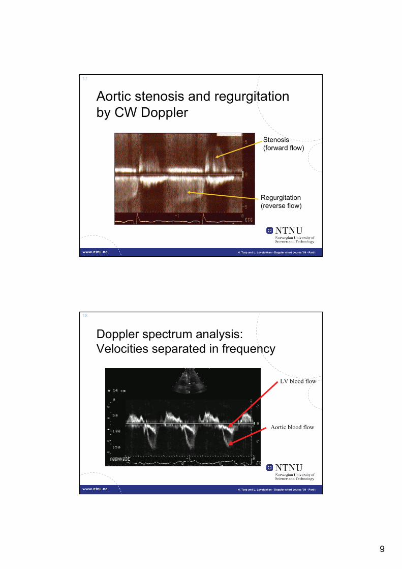
Stenosis(forward flow)

Regurgitation(reverse flow)

Aortic stenosis and regurgitationby CW Doppler

18


Doppler spectrum analysis:Velocities separated in frequency

LV blood flow

Aortic blood flow

10

19


Lecture 1 outline

• Principles and applications of CW Doppler


• Pulsed wave Doppler


20


a)

b)

Signal from a large number of red blood cells add up to a Gaussian random process

11

21


ω

G (ω)e

Power spectrum of the Doppler signal represents the distribution of velocities within the blood vessel

22


frequ

ency

time

spec

tral a

mpl

itude

Doppler spectrum

time

12

23


{ }

0)()(:

average)(ensemblevalueexpectedi

)(*)(matrixCovariance

21vector signal

,T

1 1

=⋅

−

⋅==

=

=−−−−

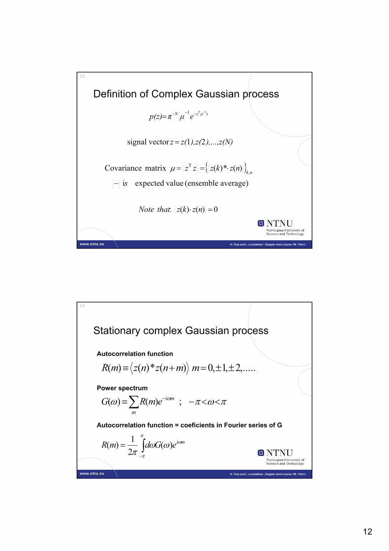
nzkzthatNote

s

nzkzzz

),...,z(N)),z(z(z

eμπp(z)

nk

zμzN T

μ

Definition of Complex Gaussian process

24


πωπω ω <<−≡∑ − ;)()(m

miemRGPower spectrum

Autocorrelation function

,......2,1,0)(*)()( ±±=+≡ mmnznzmR

∫−

=π

π

ωωωπ

mieGdmR )(21)(

Autocorrelation function = coeficients in Fourier series of G

Stationary complex Gaussian process

13

25


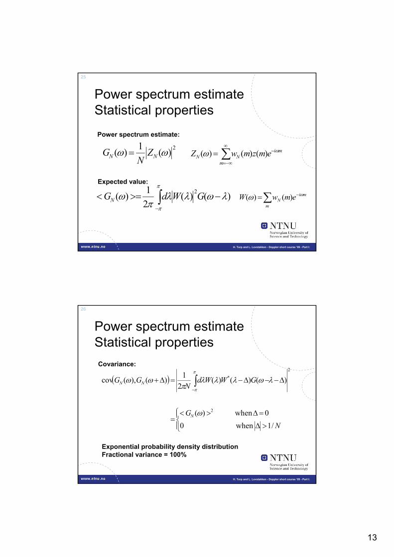
)()(21)( 2 λωλλπ

ωπ

π

−>=< ∫−

GWdGN ∑ −=m

miN emwW ωω )()(

Expected value:

∑∞

−∞=

−=m

miNN emzmwZ ωω )()()(

2)(1)( ωω NN ZN

G =

Power spectrum estimate:

Power spectrum estimateStatistical properties

26


( )

⎪⎩

⎪⎨⎧

>Δ

=Δ><=

Δ−−Δ−=Δ+ ∫−

NG

GWWdN

GG

N

NN

/1 when 00 when )(

)()()(2

1)(),(cov

2

2

*

ω

λωλλλπ

ωωπ

π

Covariance:

Power spectrum estimateStatistical properties

Exponential probability density distributionFractional variance = 100%

14

27


Clutter noise in spectral Doppler

Rectangular window Hamming window High pass filter

Interfering sidelobes from clutter signal

28


Frequency resolution versus temporal resolution

Window length 64 Window length 16

Time-bandwidth product: Δfd *ΔT = 1

15

29


Properties of power spectrum estimate

• Fractional variance = 1 independent of the window form and size

• GN(ω1) and GN(ω2) are uncorrelated when |ω1-ω2| > 1/N

• Increasing window length N gives better frequency resolution, but no decrease in variance

• Smooth window functions give lower side lobe level, but wider main lobe than the rectangular window

• Decrease in variance can be obtained by averaging spectral estimates from different data segments.

30


Lecture 1 outline





16

31


Continous Wave Doppler

ø

Single transducerPW

Double transducerCW

ø

transmit

recieve

Velocity profile, v

Artery

Range cell


Signal from all scattererswithin the ultrasound beam

Pulsed Wave Doppler

Signal from a limited sample volume

ø

Single transducerPW

Double transducerCW

ø

transmit

recieve

Velocity profile, v

Artery

Range cell


Satumora, Japan, 1957 Perroneau, Baker, Wells 1967-69

Sample volume length= cT/2

T = pulse length

32


Thermal noise

2D signal model PW DopplerPulse no1 2 .. … N

2D Fouriertransform

Doppler shift frequency [kHz

Ultr

asou

nd p

ulse

freq

uenc

y [M

Hz]

Doppler shift frequency [kHz

Pow

er

Signal from one range

Fast

tim

e

Slow time

Blood

Clutter

17

33


2D signal modelRF versus base band

Doppler shift frequency [kHz]

Blood signalClutter

Ultrasound frequency [MHz]

Doppler frequency [kHz]

Remove negative ultrasoundFrequencies by Hilbert transformor complex demodulation

•• SkewedSkewed clutterclutter filter (signal filter (signal adaptive filter) adaptive filter) cancan be be implementedimplemented withwith 1D 1D filteringfiltering

•• AxialAxial sampling sampling frequencyfrequencyreducedreduced by a by a factorfactor > 4> 4

34


Aliasing in PW Doppler

Doppler shift frequency-PRF PRF

Real signal

PRF-PRF

Complex signal

Doppler shift frequency

PRF/2

18

35


Aliasing in PW DopplerExample: Subclavian Artery

Velocity waveform restoredby stacking

36


Aliasing PW versus CW DopplerExample: Aourtic valve leakage jet

PW Doppler CW Doppler

19

37


Summary PW Doppler• Complex demodulation give direction information of

blood flow

• PW Doppler suffers from aliasing in many cardiacapplications

• Aliasing can be restored by baseline shift, or stacking, if bandwidth is limited

38


Lecture 1 outline





20

39


Is Pulsed wave Doppler based onDoppler shift or time shift?

J.A.Jensen: Estimation of blood velocities using Ultrasound

40


Continuous wave DopplerDoppler shift or time shift?

Transmitted wave

Received wave

frequency

. Reflector movingConstant speed

z(t) = z0 - v*t

tau= 2*z0/c

21

41


Pulsed wave DopplerDoppler shift or time shift?

T=1/prfT=(1-2*v/c)/prf

Transmitted wave

Received wave

frequency

df=prf

42


22

43


Doppler Short Course Doppler Short Course ‘‘0909Estimation and imaging blood flow velocity

Part II: Color Flow Imaging



44


Lecture outline• General introduction to color flow imaging

– Examples of clinical use, and a brief history lesson

• Data acquisition strategies– Acquiring the temporal sequence of samples

• Velocity estimation techniques– Estimation of Doppler signal parameters

• Clutter filtering– Attenuation of interfering signal from stationary tissue

• Display strategies in CFI

23

45


General introduction to CFI

46


Color flow imaging• Displays a color coded map of the axial blood velocity in a 2-D

or 3-D region of interest• Used in a wide range of diagnostic contexts in today's hospitals

3-D CFI of a mitral regurgitation jet2-D CFI of a carotid bifurcation

24

47


Clinical examplesMitral valve regurgitation jet Atrial septum defect shunt flow

48


More clinical examplesThyroid nodule vascularizationCarotid artery stenosis

25

49


A brief history lesson• Technology and research progressed from single-

range gate to multi-range gated Doppler, and further to 2-D Doppler imaging

Image source: J. Woo, A short History of the development of Ultrasound in Obstetrics and Gynecology, http://www.ob-ultrasound.net/history.html

Single-range gate Multi-range gate 2-D Doppler

1 2 3

1

2

3

50


A brief history lesson• Real-time CFI was first commercially available in the mid-eighties

– Aloka (1985, Japan), Toshiba (1985, Japan), Quantum (1986, US), Vingmed (1986, Norway)

Aloka SSD-880CW Vingmed CFM-700Quantum QAD-1

Source: J. Woo, A short History of the development of Ultrasound in Obstetrics and Gynecology, http://www.ob-ultrasound.net/history.html

26

51


A brief history lesson• However, real-time processing and display of color-Doppler

images in weather RADAR was available ten years earlier (!)

Source: G. R. Gray et al, Real-time color-Doppler RADAR display, Bulletin of the American Meteorological Society, vol. 56(6), 1975

Storm signs Insect signs

52


CFI acquisition and processing

27

53


CFI processing chainProcessing chain of conventional CFI

Data acquisition Clutter filtering Parameterestimation Display

• CFI data acquisition– Scanning operation and pulse sequence

• Clutter filtering (wall filtering)– Attenuating interfering signal from stationary tissue

• Doppler parameter estimation– Estimation of Doppler power, mean-frequency, and bandwidth

• Display– Color encoding of Doppler parameters

54


Mechanical scanning+ No settling time for clutter filter - Low frame rate

scanning direction

time

Electronic packet scanning- Settling time for clutter filter+ Flexible PRF without loss in frame rate

Data acquisition in CFI

Electronic continuous scanning+ No settling time for clutter filter- High frame rate, but low PRF

scanning direction

time

scanning direction

time

Packet

28

55


Interleaved packet acquisition

Beam position1234

5678

9101112

13141516

17181920

21222324

Beam position1 2 34 5 67 8 9

10 11 12

13 14 1516 17 1819 20 2122 23 24

Packet size = 4PRFmax = PRFuser

Packet size = 4PRFmax = 3*PRFuser

No interleaving 3 x beam interleaving

• Overall frame rate increased by the interleave factor• Maximum PRF limited by image depth, multiple reflections, hardware• Especially important when imaging low-velocity flow, i.e. with a low

user chosen PRF such as peripheral vascular imaging

Bea

m s

eque

nce

Reference: R. H. Chesarek, Ultrasound imaging system for relatively low-velocity blood flow at relatively high frame rates. USA, Patent no. 4888694, Quantum Medical System, Inc., 1989.

56


Packet / ensemble size in CFI• Increasing the packet size in CFI will:

+ Lead to more efficient clutter filtering+ Lower the variance of the Doppler parameters– Reduce the overall frame rate dramatically– May lead to visible artificial lags of the flow field in the image from

one side of the image to the other

• How many samples are necessary?– Application dependent, typically 8-16 samples– Cardiac imaging (deep, high dynamics): packet size = 8-10– Vascular imaging (shallow, lower dynamics): packet size = 10-16– Abdominal imaging (deep, lower dynamics): packet size = 10-12

29

57


Signal-to-noise considerations

• Similar as for PW-Doppler: total SNR ~ 1/B, spectral SNR ~ 1/B2

• The received signal from blood is proportional to the length of the transmitted pulse (incoherent sum of burstlets)

– Increase the number of pulse cycles– Decrease the pulse center frequency

• The optimal receive filter is approximatively given by a rectangular filter with length equal to the emitted pulse

– Boxcar integrator over the pulse length

• Optimize TGC to achieve a constant noise floor throughout depth

Reference: K. Kristoffersen, Optimal receiver filtering in pulsed Doppler ultrasound blood velocity measurements, IEEE Trans. Ultrason., Ferroelec., and Freq. Contr., vol. 33(1), pp. 51-58, Jan. 1986

Signal-to-noise is one of the most crucial design criteria in Doppler acquisition

58


CFI velocity estimation

30

59


Doppler signal model• The Doppler spectrum may consists of three components, clutter c,

blood b, and thermal noise n

• Typical clutter/signal level: 20 – 80 dB• Signal from blood is characterized by a complex Gaussian process

0

Doppler velocity spectrum [m/s]

Pow

er [

dB] Clutter

Blood

Noise floor

x = c + n + b x = [x(1),…,x(N)]T

60


Doppler parameter estimation

P G( )d∞

−∞= ω ω∫

G( )d

G( )d

∞

−∞∞

−∞

ω⋅ ω ωω =

ω ω

∫∫

22rms

( ) G( )dB

G( )d

∞

−∞∞

−∞

ω−ω ⋅ ω ω=

ω ω

∫∫

Time (phase) domain approaches has several qualities– Less computationally expensive– Robust in low signal-to-noise ratios– Velocity range covering the full Nyquist spectrum width

Doppler parameter estimation in CFI has focused on the first three moments of the Doppler spectrum, which equals the mean power, mean frequency, and bandwidth (rms):

However: estimating the Doppler power spectrum and integrating is not a practical solution.

31

61


Time domain formulation

j1R( ) G( )e d2

∞ ωτ

−∞τ = ω ω

π ∫

jjR( ) G( )e d2

∞ ωτ

−∞τ = ω ω ω

π ∫2 j1R( ) G( )e d

2∞ ωτ

−∞

−τ = ω ω ω

π ∫

Derivatives with respect to tau gives:

Yields time-domain expressions for power, mean frequency, and bandwidth (rms):

R(0)jR(0)

ω = −2

2 R(0) R(0)BR(0) R(0)⎡ ⎤

= −⎢ ⎥⎣ ⎦

The Wiener-Khinchin formula relates the autocorrelation function and the power spectral density function:

P R(0)=

62


The autocorrelation method

[ ]PRFPRF

PRF PRF

(T ) (0) 1 arg R(T )T T

φ −φω ≅ =

[ ]R( ) A( )exp j ( )τ = τ φ τ

R(0)j (0)R(0)

ω = − = φ

Correlation function in polar form:

Yields the following mean frequency and bandwidth estimate:

However: Accurate estimates of the derivatives of the autocorrelation function can be difficult to achieve. Therefore an alternative formulation is used:

PRF2 PRF2 2

PRF PRF

R(T )A(T )A(0) 2 2B 1 1A(0) T A(0) T R(0)

⎡ ⎤⎡ ⎤= − ≈ − = −⎢ ⎥⎢ ⎥

⎣ ⎦ ⎣ ⎦

In other words: The power, mean frequency and bandwidth of the Doppler spectrum can be found using magnitude and phase estimates of the correlation function at lags 0 and 1 (TPRF)

Reference: C. Kasai, Real-Time Two-Dimensional Blood Flow Imaging Using an Autocorrelation Technique, IEEE Transactions on Sonics and Ultrasonics, vol. 32 pp. 458-464, 1985

32

63


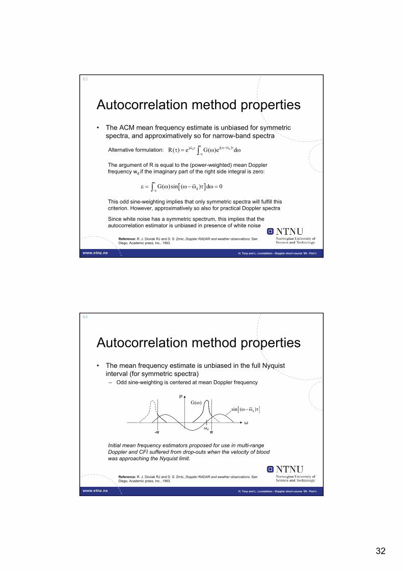
Autocorrelation method properties• The ACM mean frequency estimate is unbiased for symmetric

spectra, and approximatively so for narrow-band spectra( )dd jjR( ) e G( )e d

π ω−ω τω τ

−πτ = ω ω∫

[ ]dG( )sin ( ) d 0π

−πε = ω ω−ω τ ω =∫

Alternative formulation:

The argument of R is equal to the (power-weighted) mean Doppler frequency wd if the imaginary part of the right side integral is zero:

This odd sine-weighting implies that only symmetric spectra will fulfill this criterion. However, approximatively so also for practical Doppler spectra

Since white noise has a symmetric spectrum, this implies that the autocorrelation estimator is unbiased in presence of white noise

Reference: R. J. Doviak RJ and D. S. Zrnic, Doppler RADAR and weather observations. San Diego, Academic press, Inc., 1993.

64


Autocorrelation method properties• The mean frequency estimate is unbiased in the full Nyquist

interval (for symmetric spectra)– Odd sine-weighting is centered at mean Doppler frequency

Initial mean frequency estimators proposed for use in multi-range Doppler and CFI suffered from drop-outs when the velocity of blood was approaching the Nyquist limit.

ωdπ-π

[ ]dsin ( )ω−ω τG( )ω

ω

P

Reference: R. J. Doviak RJ and D. S. Zrnic, Doppler RADAR and weather observations. San Diego, Academic press, Inc., 1993.

33

65


Autocorrelation estimator properties

• The variance of the autocorrelation estimatorEstimate correlation function by averaging over packet

– The variance of the power estimate decreases with increasing bandwidth

– The variance of the mean frequency estimate increases with increasing bandwidth

2N2

k N

k1 Pˆvar(P) 1 R(k)N N BN=−

⎛ ⎞= − ≈⎜ ⎟

⎝ ⎠∑ P = signal power, B = signal bandwidth,

N = ensemble (packet) size

dBvar( )N

ω ∼

The variance of the autocorrelation estimates significantly improves by averaging the correlation estimates

66


Autocorrelation estimator properties

• Robust in low signal-to-noise environments– Superior to FFT-based method below ~15 dB, similar above ~15dB

• Computationally inexpensive– Ideally, in a noise free environment only two complex samples are

needed to estimate the mean frequency– In practice more samples are needed to 1) attenuate clutter, and 2)

reduce the variance of the correlation estimates

34

67


Cross-correlation method

• The velocity is proportional to the RF time shift between successive pulses

Received pulse 1Received pulse 2

Time

Am

plitu

de

PRI2vcos( )T2 zc c

θΔτ = =

max 12 sˆˆ arg max R (m) / Fτ =

SN 1

12 0 1 0 2 0k 0S

1R̂ (m,m ) r (m k)r (m k m)N

−

=

= + + +∑

maxz

PRI

ˆcv̂2 Tτ

=

τ

Reference: O. Bonnefous and P. Pesque, Time domain formulation of pulse-Doppler ultrasound and blood velocity estimation by cross correlation, Ultrasonic imaging vol. 8, pp. 73-85, 1986.

68


Properties of the cross-correlation method

• No aliasing under ideal circumstances– Signal decorrelation and lateral movement will limit this however

• Best performance for wide-band pulses– Higher resolution / lower penetration

• Axial sampling determines jitter error– Interpolation needed to find the true correlation maximum

• Time shift does not directly transfer to mean-velocity• Computationally expensive compared to

autocorrelation method

35

69


Narrow band Wide band

Autocorr.No averaging

Auto corr.1.6us averaging

Cross corr.1.6us averaging

Reference: Torp & al: Ultrasonic Symp. 93

Auto correlation vs. Cross correlation method

Example:In vivo Comparison of autocorrelation and cross-correlation for data from thehuman subclavian artery

The two methods areapproximatively equal for narrow-band pulses and withradial averaging

70


Clutter filtering

36

71


Clutter filtering• Clutter is signal from surrounding tissue due to beam side lobes

and reverberations– Can have 60-80 dB higher signal power than blood

• Blood typically has a higher velocity than tissue, i.e. higher Doppler shifts

– The two components can thus be separated by high-pass filtering the Doppler signal

0

Doppler velocity spectrum [m/s]

Pow

er [

dB] Clutter

Blood

Clutter filter

72


General clutter filter design• Clutter filters should have a high stop-band attenuation

(60-80 dB) to sufficiently attenuate clutter• Clutter filters should have a short transition region to

avoid removing signal from blood

• Several filter types have been used:– Finite impulse response (FIR) filters, Infinite impulse

response (IIR) filters, and polynomial regression filters

Normalized frequency

Stop-band

Transition region

Pass-band

Pow

er [d

B]

37

73


• The filter output y is the weighted sum of M past inputs x:

• Discard the first M output samples, where M is equal to the filter order

• Improved amplitude response when nonlinear phase is allowed

Example: Filter order M=5, packet size N=10

0 0.1 0.2 0.3 0.4 0.5-80

-60

-40

-20

0

Pow

er [d

B]


Linear phaseMinimum phase

M 1

k 0y(n) h(k)x(n k)−

== −∑

Finite impulse response (FIR) filters

Source: S. Bjærum et al, Clutter Filter Design for Ultrasound Color Flow Imaging, IEEE Trans. Ultrason., Ferroelec., and Freq. Contr., vol. 49(2), pp. 204-216, Feb. 2002

74


Linear or non-linear phase response

• Conventional color flow imaging algorithms are based on the correlation function of the filtered signal

• This means that it is safe to disregard the phase response when designing FIR clutter filters

• Without phase response constraints, an improved filter frequency response can be achieved for a given filter order

– Minimum-phase response filters have the smallest time delay and most asymmetric impulse response

(A linear transformation of the correlation function)

2 jmy x

1R (m) S ( ) H( ) e d2

πω

−π

= ω ω ωπ ∫Doppler spectrum Filter frequency response

Reference: S. Bjærum et al, Clutter Filter Design for Ultrasound Color Flow Imaging, IEEE Trans. Ultrason., Ferroelec., and Freq. Contr., vol. 49(2), pp. 204-216, Feb. 2002

38

75


Example: Chebyshev order M=4, packet size N=10

1. E. S. Chornoboy, Initialization for improved IIR filter response, IEEE Trans. Signal processing, vol. 40(3), March 1992

2. S. Bjærum et al, Clutter Filter Design for Ultrasound Color Flow Imaging, IEEE Trans. Ultrason., Ferroelec., and Freq. Contr., vol. 49(2), pp. 204-216, Feb. 2002

Infinite impulse response (IIR) filters

0 0.1 0.2 0.3 0.4 0.5-80

-60

-40

-20

0

Steady state

Step init.

Discard samples

Projection init


Pow

er [d

B]

• The filter output y is the weighted sum of past and current inputs x and past outputs y:

• Variations: Butterworth, Chebyshev, Elliptic• Filter initialization is critical to dampen the

transient response (recursive filter)• Chebyshev filter with projection initialization

preferred for color flow imaging applications

M M

k 1 k 0y(n) a(k)y(n k) b(k)x(n k)

= == − − + −∑ ∑

76


Projection matrix

• The clutter c is estimated as a least squares fitting of the signal x to a set of basis functions bk

– A projection operation from the complex vector space CN to the clutter subspace BK spanned by basis functions bk

• The clutter component is subtracted from the signal, which can formulated as a matrix operation

Regression filters

Signal space

Clutter space

b1

b2

xy

c

y = x - cb3

1. A. P. G. Hoeks et al. An efficient algorithm to remove low frequency signals in digital Doppler systems. Ultrasound Imaging, vol. 13, pp. 135-144, 1991

2. H. Torp, Clutter rejection filtering in Color Flow Imaging: a theoretical approach, IEEE Trans. Ultrason., Ferroelec., and Freq. Contr., vol. 44(2), pp. 417-424, Feb. 1997

( )M 1 Tk kk 0

y I b b x Ax− ∗=

= − =∑

K

B k kk 1

c proj (x) x, b b=

= =∑

39

77


Choice of basis functions• The choice of clutter basis functions has a large impact on

performance

0 0.1 0.2 0.3 0.4 0.5-80

-60

-40

-20

0


Pow

er [d

B]

Fourier basis:Example: N=10, clutter dim. K=3

jkn/Nk

1

Nb e , n 0,..., N 1= = −

Orthonormal and equally distributed in frequency

1. Discrete Fourier transform2. Set low frequency coefficients to zero3. Inverse Fourier transform

Analogy:

78


Legendre polynomial basis

b0 =

b1 =

b2 =

b3 =

…

• A set of orthonormal polynomials:

Pow

er [d

B]

+

+

+

+

0 0.1 0.2 0.3 0.4 0.5-80

-60

-40

-20

0

Normalized frequency( )M 1 T

k kk 0y I b b x Ax− ∗

== − =∑

Example: N=10, clutter dim. K=1-4

K

The Legendre polynomials can be generated through a Gram-Schmidt orthonormalization procedure on the polynomials xk, k=0,…,K

1

m n mn1

P (x)P (x)dx−

= δ∫

40

79


Why should clutter filters be linear?• No intermodulation between clutter and blood signal• Preservation of signal power from blood• Optimum detection (Neuman-Pearson test) includes a linear filter

y = Ax*

Filter matrix A Input vector x Output vector y

Linear clutter filter formulation

Any linear filter can be performed by a matrix multiplication of the N-dimensional signal vector x

This form includes all IIR filters with linear initialization, FIR filters, and regression filters

80


⎥⎥⎥⎥⎥⎥

⎦

⎤

⎢⎢⎢⎢⎢⎢

⎣

⎡

=

654321

654321

654321

654321

654321

0..00....00..0

bbbbbbbbbbbb

bbbbbbbbbbbb

bbbbbb

AFIR filter order M=5Packet size N=10Output samples N-M= 5

Increasing filter order + Improved clutter rejection

- Increased estimator variance

FIR filter matrix structure

41

81


Frequency response of linear filters

• The frequency response of linear filters is defined as the filter output for a single frequency complex sinusoid input

20

1H ( ) Ae ,N ωω = − π < ω< π j j(N 1) Te [1e ... e ]ω − ω

ω =

Note: The output of the filter is not in general a single frequency signal. This is only the case for FIR filters.

Note: Frequency response is only well-defined for complex signals

Reference: H. Torp, Clutter rejection filtering in Color Flow Imaging: a theoretical approach, IEEE Trans. Ultrason., Ferroelec., and Freq. Contr., vol. 44(2), pp. 417-424, Feb. 1997

82


CFI display algorithms

42

83


Power Doppler (Angio)Brightness ~ signal power

Color flowBrightness ~ signal powerHue ~ Velocity

Color flow ”Variance map”Hue & Brightness ~ VelocityGreen ~ signal bandwidth

Image example : Aortic regurgitation

Color mapping types

84


Tissue / flow arbitration

• B-mode and CFI image acquired separately due to the resolution / penetration requirements / comprimises in CFI and B-mode

• The two images are typically combined through a hard decision ofwhether to display a B-mode or color pixel Arbitration

• Post-processing is also needed in order to reduce the amount of flashing artifacts due to insufficient clutter attenuationThis decision is typically based on:

– Mean frequency and power before and after filtering– High power / low frequency (below filter cut-off) => tissue

43

85


Arbitration examples

Power-Doppler: Hard arbitration Power-Doppler: Soft arbitration

Example: Thyroid nodule vascularization

86


Topics not covered here• Advanced axial velocity estimators

– Techniques utilizing 2-D signal information

• Synthetic transmit aperture flow imaging– Lots of interesting aspects investigated

• Coded excitation in color flow imaging– When is it feasible?

• B-Flow imaging– Simultaneous acquisition of B-mode and flow images– Coded excitation to retain both resolution and penetration

• And more…

44

87


Doppler Short Course Doppler Short Course ‘‘0909Estimation and imaging blood flow velocityPart III: Advanced topics, trade-offs and limitations

2009 Ultrasonics Symposium, Rome, ItalyHans Torp, Lasse Løvstakken


88


Limitations of current Doppler / CFI techniques

45

89


Limitations of CFI

• Conventional methods suffer from several fundamental limitations that restrict its use in clinical practise

90


Data acquisition limitations

• Sufficient signal-to-noise ration vs. spatial resolution– The spatial resolution typically needs to be lowered compared to B-

mode to achieve a sufficient SNR– This leads to color blooming artifacts in CFI where the color image

smears into the B-mode image

• Frame rate vs. estimator quality vs. lateral sampling– The packet size and number of image lines is reduced in order to

achieve a sufficient frame rate for following the flow dynamics– In real-time 3-D CFI, frame rate is a particular challenge

46

91


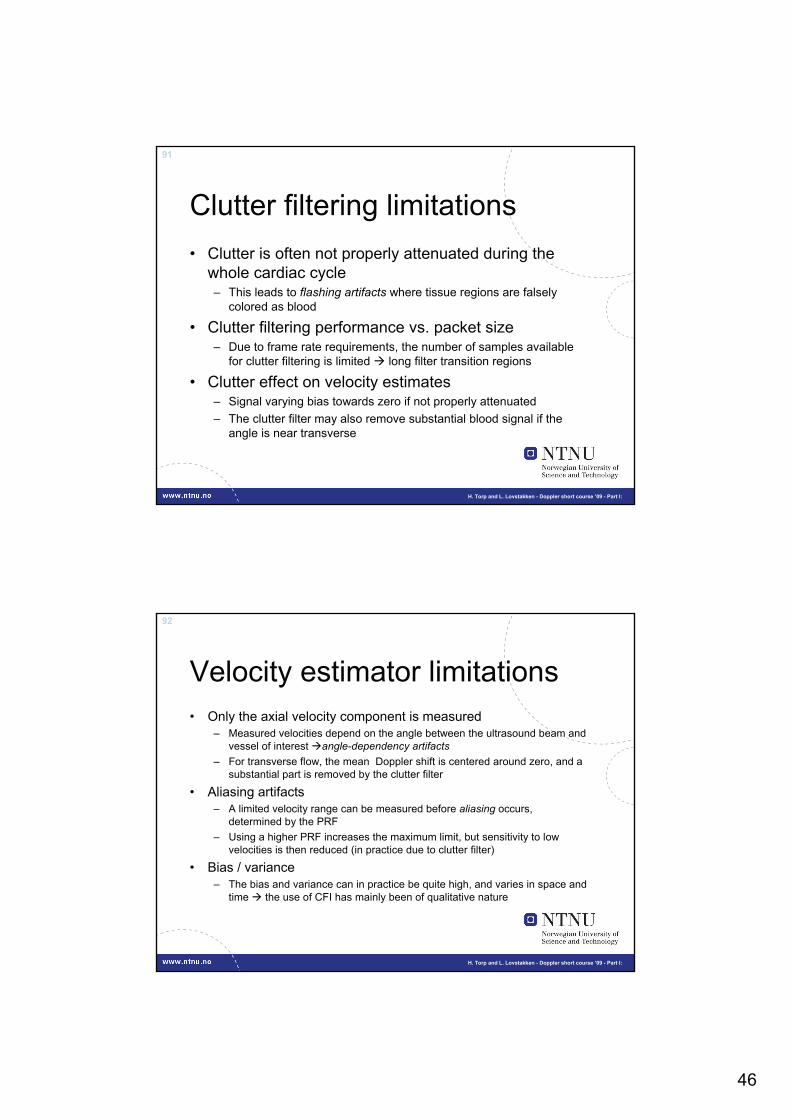
Clutter filtering limitations• Clutter is often not properly attenuated during the

whole cardiac cycle– This leads to flashing artifacts where tissue regions are falsely

colored as blood

• Clutter filtering performance vs. packet size– Due to frame rate requirements, the number of samples available

for clutter filtering is limited long filter transition regions

• Clutter effect on velocity estimates– Signal varying bias towards zero if not properly attenuated– The clutter filter may also remove substantial blood signal if the

angle is near transverse

92


Velocity estimator limitations• Only the axial velocity component is measured

– Measured velocities depend on the angle between the ultrasound beam and vessel of interest angle-dependency artifacts

– For transverse flow, the mean Doppler shift is centered around zero, and a substantial part is removed by the clutter filter

• Aliasing artifacts– A limited velocity range can be measured before aliasing occurs,

determined by the PRF– Using a higher PRF increases the maximum limit, but sensitivity to low

velocities is then reduced (in practice due to clutter filter)

• Bias / variance– The bias and variance can in practice be quite high, and varies in space and

time the use of CFI has mainly been of qualitative nature

47

93


Patient safety in Doppler imaging

94


Patient safety in Doppler imaging• Potential hazardous heating and mechanical effects restrict the allowed

acoustic output of ultrasonic imaging equipment• Acoustic output is restricted by one of the following:

– Mechanical index (MI), a measure of mechanical effects– Spatial peak temporal average intensity (Ispta), total output power, or

thermal index (TI)– Transducer surface temperature

• Heating effects are averaged for combinations of modes (duplex / triplex modes). Mechanical effects are determined by the modality withthe highest value.

The outcome: The sensitivity / penetration in Doppler modes may be severly punished from these restrictions

48

95


Mechanical effects• Mechanical effects are related to cavitation, i.e. the formation and collapse

of gas bubbles

Mechanical index:

Focal gain:

MI is measured at the axial point of maximum derated temporal averagedintensity (Ita)MI is effectively proportional to applied voltage, sqrt(f0), and inverse proportional to the F-number

r.3 sp

awf

p (z )MI

f=

a e e e 0foc

foc # #

D D D D fGR F F c

⋅= = =

λ λ ⋅(Coinciding az. an el. Foci)

Derated peak rarefactional pressure

Acoustic working frequency

96


Tissue heating• Heating occur in the tissue due to absorption, at a rate much

lower (~seconds) than the ultrasound frame rate• Spatial-peak temporal average intensity (Ispta):

• Proportional to the transmitted pulse energy• Proportional to the squared focal gain, Gfoc

• For scanned modes, the intensity contributions for overlapping beams are added

PRRT 2z

spta z0

p (t)I max PRR dtc⎡ ⎤

= ⋅⎢ ⎥ρ⎢ ⎥⎣ ⎦∫

49

97


Transducer surface heating• FDA regulations: The transducer surface may not exeed

43 deg. held towards the skin, or 50 deg. towards air

• For current transducer technology, surface heating is almost always higher than at the geometric focus1

It is typically the most limiting factor with regards to voltage / PRF / apertures

• The temperature rise for duplex and triplex modes (B-mode+CFI+PW-Doppler) is an average for a common time constant (frame rate / PRF)

Reference: 1 M. Curley, Soft Tissue Temperature Rise Caused by Scanned, Diagnostic Ultrasound, IEEE Trans., Ultrason., Ferroelect., and Freq. Contr., vol. 40(1), Jan 1993

98


Transducer surface heating• Empirical model of surface temperature:

eN

n nn 1

T(x) W T (x)=

Δ = ×Δ∑ Temperature increase for element n at position x alongthe surface

The number of times element n is fired

20 0

n n apPRF V (f ,B )T (x) g(x | x ,D , )

2⋅ ⋅β

Δ ⋅ αα

∼

Legend: PRF = pulse repitition frequency, V = voltage over element, α = measured thermalconductivity / efficiency parameter, β = measured pulse parameter, Dap=aperture width, xn=element x position

Reference: W.-S. Ohm et al, Prediction of Surface Temperature Rise of Ultrasonic Diagnostic Array Transducers, IEEE Trans., Ultrason., Ferroelect., and Freq. Contr., vol. 55(1), Jan 2008

Temperature rise is proportional to PRF, V2, g(aperture), pulse length, …

Different weighting factors, Wn. Top: PW-Doppler, bottom: scanned

Temperature rise ΔTn(x) for differenttransducer elements

50

99


PW-Doppler acoustics

• For a nonscanning situation, themaximum Ispta is close to the focal region

• The longer pulses typically used in PW-Doppler significantly increases heatingeffects

• For duplex operation (B-mode + PW-Doppler), surface temperature increase is mostly dominating

• For triplex operation (B-mode+CFI+PW-Doppler), Ispta or surface temperature willdominate

0 0.5 1 1.5 20

1000

2000

3000

4000

MI

Ispt

a03

[mW

/cm

2 ]

PW-Doppler: MI vs. Ispta.3 for varying pulse lengths

2.5 periods5 periods10 periodsFDA limits

Outcome: PW-Doppler is typically Ispta limited, exceptionsinclude very low PRFs, low frequencies, and narrow focusing

Setup: Linear array, f0 = 5MHz, FNtx = 2.5, txFocus 4 cm, PRF = 8kHz

2.5 periods

5 periods

10 periods

100


Color Flow Imaging acoustics• For a scanning situation, the maximum

Ispta is close to the surface• Similar characteristics for phased-array

(cardiac) probes as for linear array(vascular) probes

• Duplex operation adds heating effects from B-mode

• Generally surface temperature limited• MI limited only for short pulses, low

frequencies and PRFs, narrow focusingSetup: Linear array, f0 = 5MHz, FNtx = 2.5, txFocus 4 cm, PRF = 4kHz, 2 cm ROI width, 50 beams. NB: B-mode values not added

CFI is typically transducer surface temperature limited.Exceptions include very low PRFs, low frequencies, and narrow focusing

0 0.5 1 1.5 20

500

1000

1500

2000

MI

Ispt

a03

[mW

/cm

2 ]

CFI: MI vs. Ispta.3 for varying pulse lengths

2.5 periods5 periods10 periodsFDA limits

2.5 periods

5 periods

10 periods

51

101


Surface temperature comparison

• An example of surfacetemperature prediction for PW vs. CFI for the same aperture / tx-focus

• CFI generates a higher surfacetemperature then PW-Dopplerdue to:

– Aperture overlap during scanning, i.e. individual elements are excitedmore often,

– The imaging PRF is often higher in CFI than for PW-Doppler

0 0.5 1 1.5 20

5

10

15

20

25

30

MI

Tem

pera

ture

incr

ease

[deg

]

CFI: 2.5 periodsCFI: 5 periodsCFI: 10 periodsPW: 2.5 periodsPW: 5 periodsPW: 10 periods

Common setup: Linear array, f0 = 5MHz, FNtx = 2.5, txFocus 4 cm

CFI: PRF_img = 16kHz, PRF=4kHz, Np=12, 2 cm ROI width, 50 beams.

PW: PRF_PW = 8kHz, Np=64

NB: B-mode values not added

102


Patient safety summary• Transducer surface heating is currently the main limitation in CFI and B-

mode+PW-Doppler, while Ispta is the main limitation in CW- and PW-Doppler (without B-mode)

– MI limitations might occur for low PRFs, short pulses, and narrow focusing

• For an equal PRF, the temporally average transmitted energy is distributed over a larger spatial region for scanned modes than for PW-Doppler:

– Lowering overall tissue heating effects for scanned modes– Bringing the maximum temperature close to the transducer for scanned modes– Especially the case for 3-D imaging

• These rules of thumb apply to both linear array (vascular) as well as phased array (cardiac) imaging

52

103


Coded excitation in Doppler• Using non-linear phase-modulation can

increase the pulse length without reducingthe bandwidth, and may therfore be used to increase the amount of transmitted energy

• Deconvolution filtering on receive restoresthe phase to retain axial resolution

• The theoretical improvement in SNR is equalto the time-bandwidth product of thetransmitted waveform, TB.

– I.e., for a given bandwidth, doubling the pulse length by coding may theoretically double the SNR

Reference: T. Misaridis and J. A. Jensen, Use of Modulated Excitation Signals in Medical Ultrasound. Part I: Basic Concepts and Expected Benefits, IEEE Trans., Ultrason., Ferroelect., and Freq. Contr., vol. 52(2), Feb 2005

104


When is coded excitationapplicable in Doppler modes?• Codes are in general applicable only when MI-limited• As previously indicated, heating effects are typically

prominent and will severely limit the advantage ofcodes in Doppler modes

• Disregarding surface heating, a potential mighthowever exist for codes in CFI– More efficient transducer materials– Active cooling– Unfocused imaging (MI ~ Gfoc, Ispta ~ Gfoc

2, Gfoc= 1)

53

105


Advanced axial velocity estimators

106


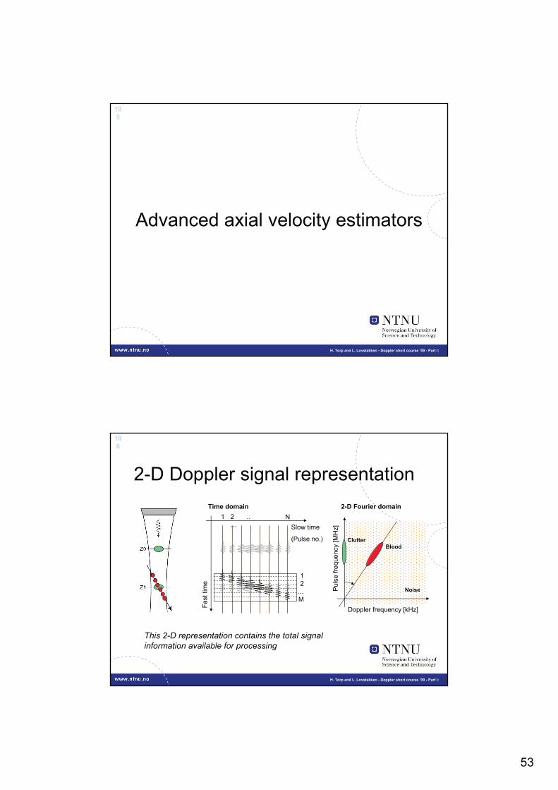
2-D Doppler signal representation

Doppler frequency [kHz]

Pul

se fr

eque

ncy

[MH

z]

2-D Fourier domain

ClutterBlood

Noise

1 2 .. …

N

12

…M

Fast

tim

e

Slow time

(Pulse no.)

Time domain

This 2-D representation contains the total signal information available for processing

54

107


�‚

Ultrasoundfrequency

Dop

pler

shift

Vessel wall signal

Blood signal

Receiver noise

�¹

�¤

Nyq

uist

rang

e

[kHz]

2.24

4.48

0

-2.242.5 5

[MHz]

2-D spectrum example

Estimated2D spectrum

Estimated1D spectrum

Theoretical2D spectrum

108


Velocity matched spectrum algorithm for PW-Doppler

Pulse no1 2 .. … N

Doppler shift frequency [kHz]

Ultr

asou

nd p

ulse

freq

uenc

y [M

Hz]

Velocity

Pow

er

55

109


Blood velocity spectrumSubclavian Artery

-100

-50

50

100

-100

-50

50

100

Conventional spectrum Velocity matched spectrum

110


Advanced velocity estimation in Color Flow Imaging• The autocorrelation approach is a a narrow-band

technique that only utilizes a portion of the signal information available

• Several wide-band velocity estimators have beenproposed, some examples:– Cross-correlation technique– 2-D spectral processing techniques– Wide-band maximum likelihood estimator

• These methods may outperform the ACM withregards to accuracy and aliasing limit

56

111


Disadvantages of wide-bandprocessing• Wide-band, i.e. short pulses are needed, which may

lead to SNR problems

• Decorrelation limits the practical velocity range thatmay be tracked beyond the Nyquist range

• Substantially increased computational load

112


Adaptive clutter filtering

57

113


Adaptive clutter filtering in CFI• An adaptive filter has a data

dependent response• Adapting the clutter filter to

clutter characteristics may:– Reduce flashing artifacts by more

effecively attenuating clutter– Remove less blood signal

throughout the cardiac cycle

• Especially relevant in:– Low-flow environments – Excessive tissue movement

environmentsExample: Flashing artifacts when imaging an healthy carotid artery and thyroid (low PRF)

114


The downmixing approachAlgorithm:• Estimate the main tissue Doppler frequency, ωt

• Downmix the signal with ωt prior to conventional clutter filtering

Reference: L. Thomas and A. Hall, An improved wall filter for flow imaging of low velocity flow, Proceedings of the IEEE Ultrasonics Symposium, 1994

58

115


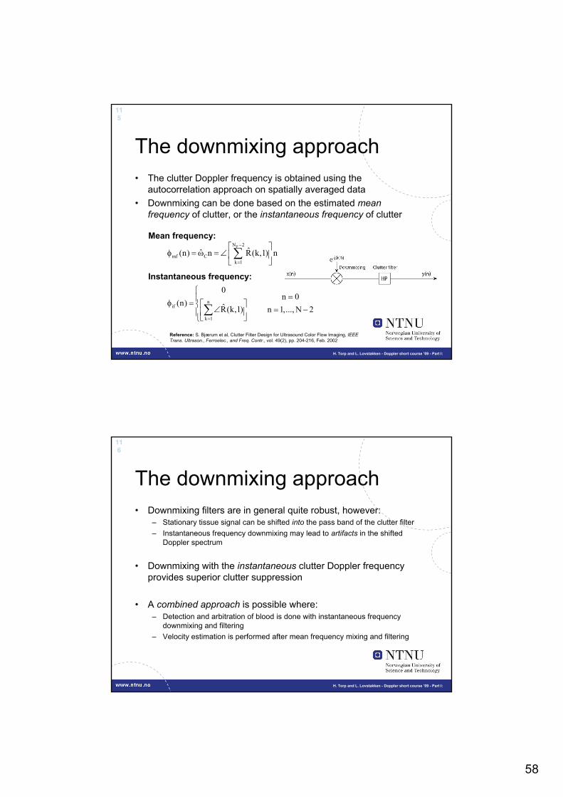
• The clutter Doppler frequency is obtained using the autocorrelation approach on spatially averaged data

• Downmixing can be done based on the estimated mean frequency of clutter, or the instantaneous frequency of clutter

The downmixing approach

nif

k 1

0n 0

(n)R̂(k,1) n 1,..., N 2

=

⎧=⎪φ = ⎡ ⎤⎨ ∠ = −⎢ ⎥⎪⎣ ⎦⎩

∑

PN 2

mf Ck 1

ˆˆ(n) n R(k,1) n−

=

⎡ ⎤φ = ω = ∠⎢ ⎥

⎣ ⎦∑

Mean frequency:

Instantaneous frequency:

Reference: S. Bjærum et al, Clutter Filter Design for Ultrasound Color Flow Imaging, IEEE Trans. Ultrason., Ferroelec., and Freq. Contr., vol. 49(2), pp. 204-216, Feb. 2002

116


The downmixing approach• Downmixing filters are in general quite robust, however:

– Stationary tissue signal can be shifted into the pass band of the clutter filter– Instantaneous frequency downmixing may lead to artifacts in the shifted

Doppler spectrum

• Downmixing with the instantaneous clutter Doppler frequency provides superior clutter suppression

• A combined approach is possible where:– Detection and arbitration of blood is done with instantaneous frequency

downmixing and filtering– Velocity estimation is performed after mean frequency mixing and filtering

59

117


The eigen-based conceptBackground• The clutter contribution to signal variation is different then from blood

Typically: The clutter component is more dominant (higher energy) and infers more low-frequency variation than blood

Filter principle• Principal component analysis (PCA) / the Karhunen Loeve

expansion (KLE) separates the main sources of variation• By selecting the modes of variation based on a priori knowledge of

clutter, a signal basis can be found and used to attenuate clutter

118


Eigen-based algorithm1. Estimate correlation matrix

Average in a spatial region

2. Signal decompositionEstimate eigenvectors and eigenvalues, i.e. the orthogonal signal basis functions in PCA

3. Identify clutter eigen-componentsBased on a priori assumptionsFor instance the most dominant in energy

4. Form filter matrix and filterRegression / projection filtering approach

60

119


The eigen-based formulas• Signal model consists of up to three independent components, clutter

c, noise n, and optionally blood b

• The signal correlation matrix is estimated by spatial averaging

• The clutter is represented by the orthonormal basis given by selectedeigenvectors of the signal correlation matrix

• Filtering is performed as for regression filters through projection

x c n b= + +

M Tx m mm 1

1R̂ x xM

∗=

= ∑

{ }D kNk k k lk 1

, k l

0, k lx e , E ∗

=

λ =

≠

⎧= γ γ γ = ⎨⎩

∑

cK Tk kk 1

P I e e∗=

= −∑

x c n bR R R R= + +

120


An eigen-spectrum example

Eigen-spectrum for 1) tissue+noise, and 2) tissue+blood+noise

Image example: Epicardial imaging of porcine myocardium at 14 MHz

Blood component

Eigen-spectrum is sorted on increasing eigenvector mean frequency

61

121


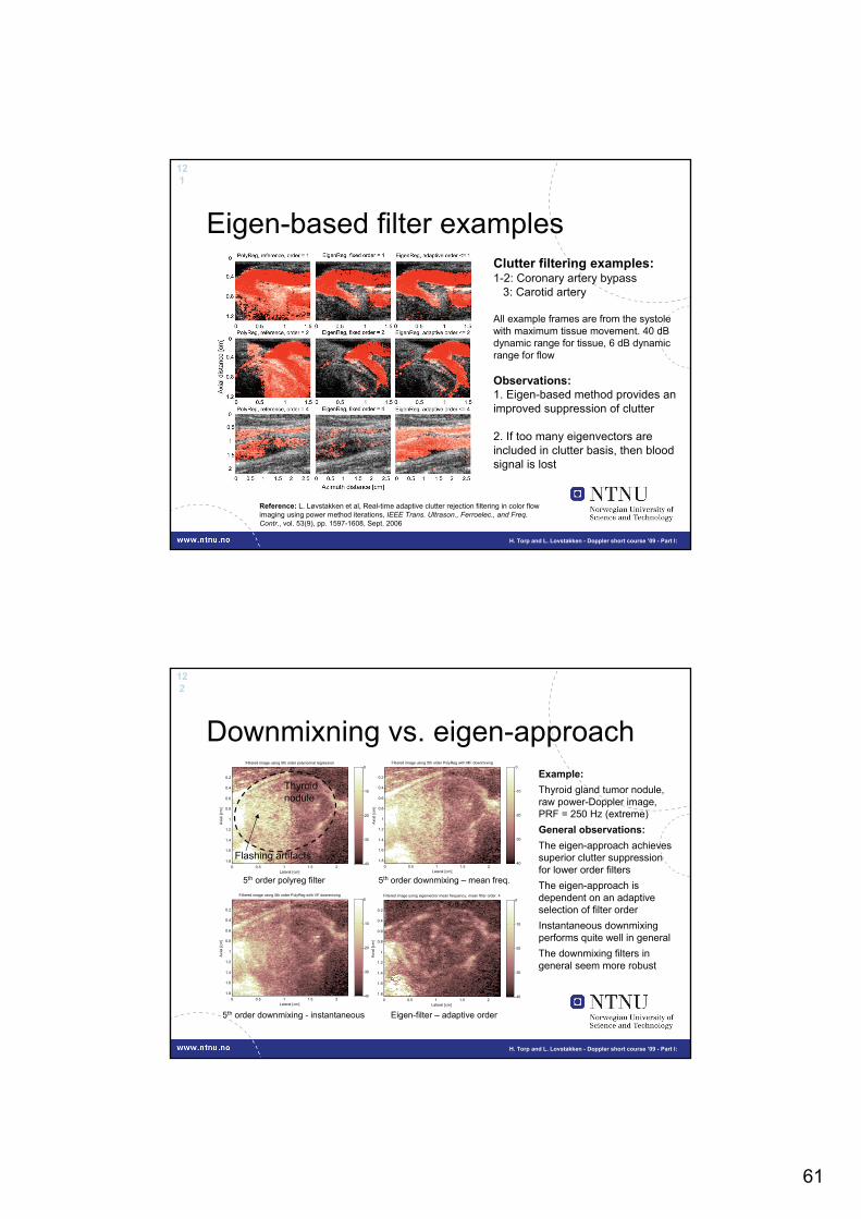
Eigen-based filter examplesClutter filtering examples:1-2: Coronary artery bypass

3: Carotid artery

All example frames are from the systole with maximum tissue movement. 40 dB dynamic range for tissue, 6 dB dynamicrange for flow

Observations:1. Eigen-based method provides an improved suppression of clutter

2. If too many eigenvectors areincluded in clutter basis, then bloodsignal is lost

Reference: L. Løvstakken et al, Real-time adaptive clutter rejection filtering in color flow imaging using power method iterations, IEEE Trans. Ultrason., Ferroelec., and Freq. Contr., vol. 53(9), pp. 1597-1608, Sept. 2006

122


Downmixning vs. eigen-approach

Lateral [cm]

Axi

al [c

m]

Filtered image using 5th order PolyReg with VF downmixing

0 0.5 1 1.5 2

0.2

0.4

0.6

0.8

1

1.2

1.4

1.6

1.8-40

-30

-20

-10

0

Lateral [cm]

Axi

al [c

m]

Filtered image using 5th order polynomial regression

0 0.5 1 1.5 2

0.2

0.4

0.6

0.8

1

1.2

1.4

1.6

1.8-40

-30

-20

-10

0

Lateral [cm]

Axi

al [c

m]

Filtered image using eigenvector mean frequency, mean filter order: 4

0 0.5 1 1.5 2

0.2

0.4

0.6

0.8

1

1.2

1.4

1.6

1.8-40

-30

-20

-10

0

Lateral [cm]

Axi

al [c

m]

Filtered image using 5th order PolyReg with MF downmixing

0 0.5 1 1.5 2

0.2

0.4

0.6

0.8

1

1.2

1.4

1.6

1.8-40

-30

-20

-10

0

Example:Thyroid gland tumor nodule, raw power-Doppler image, PRF = 250 Hz (extreme)General observations:The eigen-approach achieves superior clutter suppression for lower order filtersThe eigen-approach is dependent on an adaptive selection of filter orderInstantaneous downmixingperforms quite well in generalThe downmixing filters in general seem more robust

5th order downmixing - instantaneous

5th order downmixing – mean freq.

Eigen-filter – adaptive order

5th order polyreg filter

Thyroid nodule

Flashing artifacts

62

123


Comparison movies

4th order polyreg filter 4th order downmixing - instantaneous Eigen-filter – adaptive order

Example:Thyroid gland tumor nodule, raw power-Doppler image, PRF = 250 Hz (very low)

124


Summary – adaptive clutter filtering• Eigen-based filtering can provide superior clutter suppression for

low filter orders in regions with excessive tissue motion, however:– The filter order must be chosen adaptively for different regions of the

image for robust performance– Spatial averaging of the correlation matrix estimate smoothes the

resulting flow images

• Downmixing filtering can provide an improved suppression of clutter in general, however:– Stationary signal may be shifted into the pass band– Artifacts may appear in the Doppler spectrum when using a varying

(instantaneous) downmixing frequency

63

125


Doppler Short Course Doppler Short Course ‘‘0909Estimation and imaging of blood flow velocity

Part IV: Future directions



126


Lecture outline• 2-D vector velocity imaging of blood

– Vector-Doppler, speckle tracking, echo-PIV

• High frame rate Color Flow Imaging– Parallel beamforming, plane-wave imaging, synthetic aperture flow

imaging, multi-transmit CFI

• Real-time 3-D ultrasound applications– 3-D color flow imaging, high-PRF 3-D imaging of mitral valve

leakage

64

127


2-D velocity vector imaging

128


2-D blood vector velocity mapping

• Vector-Doppler techniques– Combine Doppler shift from spatially separated transmit / receive

apertures

• Speckle imaging / tracking techniques– Visualization of speckle pattern movement– Tracking of speckle pattern movement

• Transit-time broadening techniques– The bandwidth of the Doppler signal is related to the lateral velocity

component

• Synthetic aperture techniques– Beamforming and cross-correlation along arbitrary lines. Choosing

the direction of maximum correlation

65

129


Vector-Doppler techniques

• Compound Doppler techniques– Combine Doppler shift from several physically / electronically

separated transmit / receive apertures

• Lateral oscillation techniques– Common transmit aperture, spatially separated receive apertures

created electronically using “non-uniform” apodization functions– Transverse oscillation method (TO) (Jensen 1998)– Spatial quadrature method (SQ) (Anderson 1998)

130


Velocity components:

Vx = (λ/2) (f2 - f1)

Vz = (λ/2) (f2 + f1)

f2f2 + f1

f2 – f1

TX aperture Right RX ap.

f1

Left RX ap.

r2r1

US patent 93 Anne Hall, GE, Crossing beam Color flow imagingExpanding aperture

f1 : Doppler shift left aperture

f2 : Doppler shift right aperture

Compound Doppler methodwith common transmit beam

66

131


TX aperture Right RX aper.Left RX aper.

r2r1

reven = 0.5 (r1 + r2 )

rodd = -0.5 j ( r1 - r2 )

Reconstruction:r1 = reven + j roddr2 = reven - j rodd

Spatial quadrature technique

reven rodd

Reference: M. E. Anderson. Multi-dimensional velocity estimation with ultrasound using spatial quadrature. IEEE Trans., Ultrason., Ferroelect., and Freq. Contr., vol. 45(3), pp. 852-861, May 1998

An oscillation in the lateral field is created using a non-uniform receive apodization function (left/right receive)

The left / right receive apertures are separated using quadrature relations

132


Transverse oscillation techniqueAn oscillation in the lateral field is created using a non-uniform receive apodization function (left/right receive)

The left / right receive apertures are separated by sampling beams one quarter lateral wavelength apart

TX aperture Right RX aper.Left RX aper.

References:J. A. Jensen and P. Munk. A new method for estimation of velocity vectors. IEEE Trans., Ultrason., Ferroelect., and Freq. Contr., vol. 45(3), pp. 837-851, May 1998J. Udesen and J. A. Jensen. Investigation of Transverse Oscillation Method. IEEE Trans., Ultrason., Ferroelect., and Freq. Contr., vol. 53(5), pp. 959-971, May 2006

λlat / 4

reven rodd

67

133


10 20 30 40 50 600

0.2

0.4

0.6

0.8

1

1.2

Transducer element

Apo

disa

tion

mag

nitu

de

10 20 30 40 50 60

-150

-100

-50

0

50

100

150

Transducer element

Apo

disa

tion

phas

e [d

eg]

AevenAoddA2

AevenAoddA2

Compound Doppler vs TO comparison

• SNR-ratio analysis:TO method - 0.11 dB

• Mirror spectral energy: 29 dB• No significant velocity bias

when using autocorrelation method

Separation error

134


Summary of vector Doppler methods

• Spatial quadrature and compound Doppler areidentical methods

• Transverse oscillation method is approximatelyequal to compound Doppler method for smallapertures and narrowband pulses

• All three methods give approximatively equalperformance for typical aperture / pulse bandwidths

68

135


Blood speckle imaging• The speckle pattern from blood flow signal is isolated by high-

pass filtering the Doppler signal• The movement of this speckle pattern is correlated to the

movement of blood

Figure: B-mode image of carotis artery and corresponding filtered image showing the blood flow speckle pattern utilized in BFI

Blood flow echospeckle pattern

Tissue echospeckle pattern

136


• Speckle pattern images of moving blood is captured at a highframe rate, and is played back in slow motion

• The movement of the blood flow speckle pattern can then be visually tracked from image to image

Blood Flow ImagingSpeckle movement visualization

Figure: A visualizationof the speckle patternmovement from blood in a carotid bifurcation

Speckle images aresuperimposed ontoconventional Dopplerimages

Reference: L. Lovstakken et al. Blood Flow Imaging - A New Real-Time, 2-D Flow Imaging Technique. IEEE Trans., Ultrason., Ferroelect., and Freq. Contr., vol. 53(2), pp. 289-299, Feb 2006

69

137


BFI - signal processing

• High-pass filtering produce signal from blood– Time-invariant FIR filters preserve speckle pattern

similarities

• B-mode processing produces speckle images• Amplitude normalization

– Reduce signal power discontinuities between frames

• Combine with CFI– Modulate the parametric color images with speckle

pattern images– Interpolate color images in time to match the number

of speckle images

Acquisition

High PassFiltering

EnvelopeDetection

DynamicCompression

AmplitudeNormalization

CFI / PDProcessing

Mean powerEstimate

Display

Mean freq.Estimate

1. 2. 3. 4. 5. 9.

6. 7.

8.

Figure: Normalization needed to reducediscontinuties between image frames

Not normalized

Normalized

138


BFI example 1 – vascular imaging

Vascular imagingImaging of a stenosed carotid bifurcationLeft: Power Doppler + speckle, right: CFI + speckle

70

139


BFI example 2 – coronary bypass surgery

Intraoperative imaging in cardiothoracic surgeryImaging of a proximally occluded (snared) LIMA-LAD bypassanstomosis, using CFI (left) and BFI (right)

140


Speckle tracking of blood• Tracking speckle pattern between subsequent frames, speckle

displacement is given by best match

∑∑= =

++−=l

i

k

jn jiXjiXn

1 10 ),(),(),,( βαβαε

Sum of Absolute Differences (SAD):Block matching algorithm Real-time operation feasible (special purpose multimedia instructions)Displacement given for minimal SAD:εmin = (αm, βm)

nTzx

V mmn

22 )()( Δ+Δ=

βαzx

m

mn Δ

Δ=

βαϑ arctan

(α,β)

X0

Xn

G. E. Trahey et al. Angle Independent Ultrasonic Detection of Blood Flow. IEEE Trans., Biomed. Eng., vol. 34(12), pp. 965-967, Dec 1987

L. N. Bohs et al. Speckle tracking for multi-dimensional flow estimation. Ultrasonics, vol. 38, pp. 369–375, 2000

71

141


Speckle tracking challenges

• Speckle decorrelationThe speckle pattern decorrelates rapidly due to:a) Spatial and temporal velocity gradientsb) Non-laminar flowc) Out-of-plane movements

• Clutter filtering– Doppler-based high-pass filtering removes blood signal for near-

transversal flow– Reduces SNR, and influences the speckle appearence

142


Speckle tracking acquisition A very high frame rate is needed due to the rapid decorrelation• Interleaved / parallel beam acquisition

– Speckle region frame rate equal to the user chosen PRF– Two-way resolution / penetration– Time lag across image as in conventional color flow imaging

• Plane wave acquisition– Single unfocused transmit beam, all receive channels available– Continuous acquisition, processing from frame to frame– High overall frame-rate (~100 Hz), no time lags across image– Reduced resolution and penetration coded excitation

72

143


Plane wave emission• Unfocused transmit beam• Receive channel data

available• One speckle image for each

transmit pulse• 13 bit barker codes• Resolution ~ 1x1 mm• Frame-to-frame clutter filtering• Frame rate 100 Hz

J. Udesen et al, “Fast Blood Vector Velocity Imaging: Simulations and Preliminary in vivo Results”, Proceedings of IEEE UltrasonicsSymposium, New York 2007

144


Speckle tracking vs. vector-Doppler• By simulating ultrasound signals from realistic flow fields obtained using

computational fluid dynamics, experimental methods can be evaluated and compared statistically in a controlled manner

A. Swillens et al., Ultrasonics Symposium 2008, Beijing, China

Vector-Doppler

Speckle tracking

CFD reference

73

145


Speckle tracking vs. crossed-beamvector Doppler• Simulated data from a carotid artery bifurcation model (CFD)• Comparison movie for a clutter filtered example at 2kHz PRF

Speckle tracking Crossed-beam vector Doppler

A. Swillens et al. Oral presentation given at blood flow session Wednesday, 23. Aug.

146


Clutter filtering in 2-D velocity estimation

• Doppler-based clutter filtering will remove signal from blood as the beam-vessel angle approaches 90°

• Vector-Doppler– Signal drop-out for tx/rx aperture from one side

• Speckle tracking– Signal drop-out for near transversal flow– Remaining signal becomes band pass also laterally lateral

oscillations

One of the main challenges in 2-D velocity estimation

74

147


Clutter filtering effect on the speckle images• Axial and lateral object movement is equal to a rotation of the

system point spread function around the kz-ω and kx-ω axes in k-space

• Ideal clutter filter removes all signal below a threshold ω-plane• The remaining signal may become band-pass in both kz and kx

Remaining signal

K-space representation:

Threshold plane

FIR filtered, ~60 deg

FIR filtered, ~90 deg

148


Echo particle image velocimetry(Echo-PIV)• Tracking the movement of

small concentrations ofinjected contrast bubbles

• Avoids problems with clutterfiltering and low SNR

• Can be used to estimateflow-derived parameters such as wall shear rate

Reference: G.-R. Hong et al. Characterization and Quantification of Vortex Flow in the Human Left Ventricle by Contrast Echocardiography Using Vector Particle Image Velocimetry, JACC: Cardiovascular Imaging, Volume 1, Issue 6, November 2008

Example: Left ventricle flow patterns by Echo-PIV

75

149


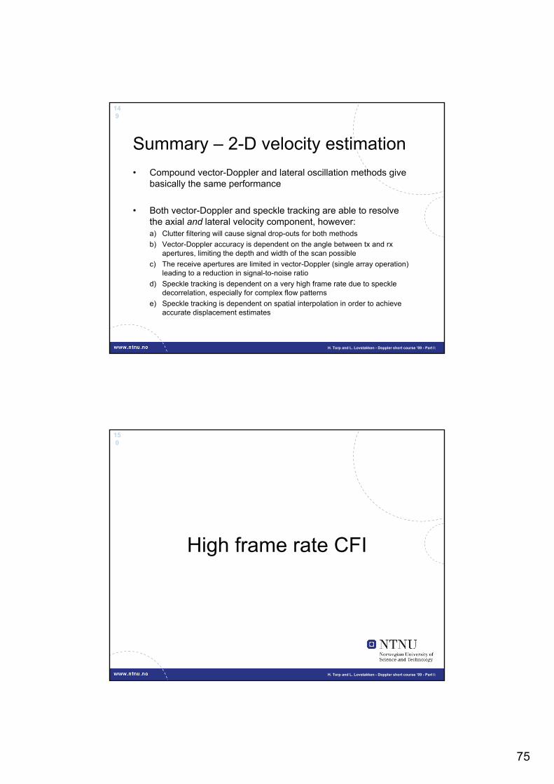
Summary – 2-D velocity estimation• Compound vector-Doppler and lateral oscillation methods give

basically the same performance

• Both vector-Doppler and speckle tracking are able to resolve the axial and lateral velocity component, however:a) Clutter filtering will cause signal drop-outs for both methodsb) Vector-Doppler accuracy is dependent on the angle between tx and rx

apertures, limiting the depth and width of the scan possiblec) The receive apertures are limited in vector-Doppler (single array operation)

leading to a reduction in signal-to-noise ratiod) Speckle tracking is dependent on a very high frame rate due to speckle

decorrelation, especially for complex flow patternse) Speckle tracking is dependent on spatial interpolation in order to achieve

accurate displacement estimates

150


High frame rate CFI

76

151


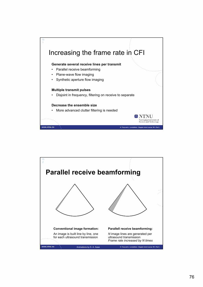
Increasing the frame rate in CFIGenerate several receive lines per transmit• Parallel receive beamforming• Plane-wave flow imaging• Synthetic aperture flow imaging

Multiple transmit pulses• Disjoint in frequency, filtering on receive to separate

Decrease the ensemble size• More advanced clutter filtering is needed

152


Parallel receive beamforming

Animations by S. A. Aase

Conventional image formation:An image is built line by line, onefor each ultrasound transmission

Parallell receive beamforming:N image lines are generated per ultrasound transmissionFrame rate increased by N times

77

153


Parallel receive beamforming

+ N image lines are generated per ultrasound transmission, i.e. frame rate increasesby N. Based on traditional focused beams on transmit.

- The curvature of focused transmit beams leads to a Doppler angle varyingacross the group of parallel receive beams

- For a large number of PRB the transmit aperture becomes very small

Reference: T. Hergum et al., Reducing Color Flow Artifacts caused by Parallel Beamforming, IEEE Trans. Ultrason., Ferrielect. And Freq. Contr. submitted, 2009

Find out more at the poster presentation by T. Hergum in the Beamforming session at this years conference

154


Plane-wave imagingPlane-waves are unfocused ultrasound beams, without curvature over a limited depth

One transmitted plane-wave can illuminate a large spatial region so that a high numberof parallel receive beams can be utilized

Due to the flat curvature, image artifactsnormally associated with parallel receivebeamforming for focused beams areavoided

Trade-off: A significant loss in transmittedpressure compared to focused beams

Unfocused pulse

Focused pulse

depth

depth

78

155


What is the difference?An illustration of the frame rate difference for the same amountof image lines (fully sampled). Playback is at 20% of real-time.

Equivalent to current high-endacquisition, 2x parallel beams

Plane wave imaging, 16x parallelbeams (both B-mode and CFI)

Image example:

Neonate heartwith an atrium-ventricularseptum defect. Parasternalcross-section.

More examples areshown at this yearsconference, Wednesday 23. Sept at the oral BloodFlow session

156


Synthetic apertureflow imaging• One emission results in a complete

image with low resolution and SNR• By combining several low-resolution

images a high-resolution image is produced

Pros and cons+ Continuous acquisition+ Flexible beamforming- SNR issues- Computational demands- Motion artifacts due to inadequate

compensation of movement for high-resolution images

Reference: S. I. Nikolov and J. A. Jensen, In-Vivo Synthetic Aperture Flow Imaging in Medical Ultrasound, IEEE Trans. Ultrason., Ferrielect. And Freq. Contr. vol. 50, no. 7, July 2008

79

157


Multiple transmit pulses

Reference: N. Odderhede et al, Multi-Frequency Encoding for Fast Color Flow or QuadroplexImaging, IEEE Trans. Ultrason., Ferrielect. And Freq. Contr. vol. 55, no. 4, April 2008

Pros and cons+ Increases the frame rate by N+ Conventional focused beams+ May be combined with parallel receive

beamforming- Varying estimator quality for different

frequency bands- Varying Nyquist velocity for each band- Varying SNR for each band

• Emit N wide-band transmit pulses simultaneously in different directions

• Filter signals from disjoint (narrow-band) frequencybands on receive

158


Real-time 3-D imaging

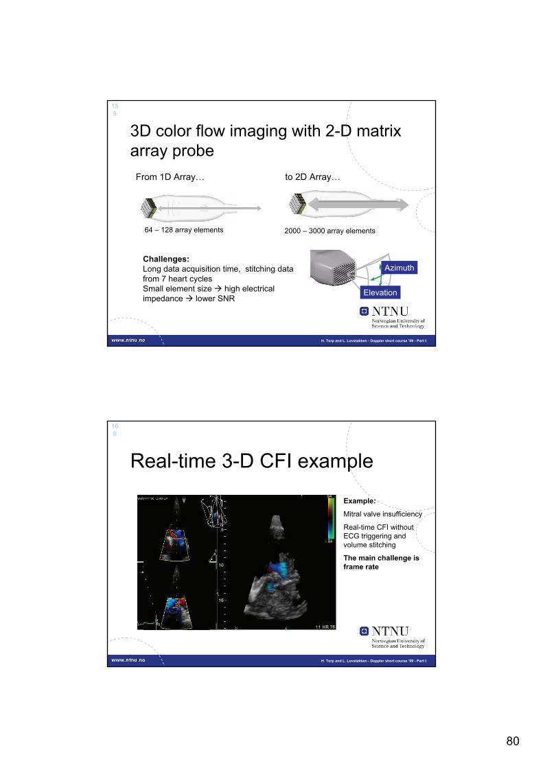
80

159


3D color flow imaging with 2-D matrixarray probe

Azimuth

Elevation

Challenges:Long data acquisition time, stitching data from 7 heart cyclesSmall element size high electricalimpedance lower SNR

64 – 128 array elements

From 1D Array… to 2D Array…

2000 – 3000 array elements

160


Real-time 3-D CFI example

Example:

Mitral valve insufficiency

Real-time CFI without ECG triggering and volume stitching

The main challenge is frame rate

81

161


Real-time 3-D CFI example

Example:


Real-time CFI without ECG triggering and volume stitching

6-slice view – notice the banana shaped leakage in the mitral valve indicated by the green color (increased Doppler bandwidth)

New information!

162


Estimation of Valvular regurgitationArea by 3D HPRF Doppler

T. Hergum, T. Skaug

Mitral valve 3-D beam pattern


Valvular regurgitant jet area can be quantified by isolating the Dopper signal power from the jet over the whole leakage area relative to a knownreference signal from the center of the jet (vena contracta)

82

163


In vitro results

0 10 20 30 400

5

10

15

20

25

30

35

40

45CSA estimation

True area [mm2]

Est

imat

ed a

rea

[mm

2 ]

Over-estimation for small areas

Under-estimation for large areas

Azimuth [mm]

Azi

mut

h [m

m]

In vitro vena contracta

-5 0 5

-6

-4

-2

0

2

4

60

5

10

15

20

25

30

164


In vivo - compared to MRI

Regurgitant volume (RV) = area * velocity-time-integral

• Vena contracta positiondetermined with PW Doppler.

• Jet power isolated withhigh pulse repetitionfrequency (HPRF).

• Acquire 3D HPRF data.• Obtains jet geometry,

cross sectional area,and regurgitant volume.

• Small leakagesoverestimated whencompared to MRI. This is expected due to thefinite beam width.

Look for the narrow bandwidth of vena contracta

83

165


Thanks for your attention!(We hope you enjoyed the show)

AcknowledgementsA. Støylen (NTNU), A. Heimdel (GE Vingmed), S. Bjærum (GE Vingmed), K. Kristoffersen (GE Vingmed), T. Hegrum (NTNU), J. Crosby (NTNU), F. Orderud (NTNU), J. Udesen (DTU), J. U. Voigt, S. A. Aase (NTNU), A. Swillens (UGent), P. Segers (UGent), and more…

166


Reference listTextbooks used for all lectures 1. Angelsen, B.A.J. and H. Torp, Ultrasound Imaging: Waves, Signals, and Signal

Processing. Vol. 2. 2000, Trondheim: Emantec AS.

2. Doviak, R.J. and D.S. Zrnic, Doppler RADAR and weather observations. Second edition ed. 1993, San Diego: Academic press, Inc.

3. Jensen, J.A., Estimation of Blood Velocities Using Ultrasound. 1996, New York: Cambridge University Press.

4. Cobbold, R.S.C., Foundations of Biomedical Ultrasound. 2007, New York: Oxford University Press, Inc.

84

167


Reference listPW-Doppler / Color flow imaging1. Kasai, C., et al., Real-Time Two-Dimensional Blood Flow Imaging Using an

Autocorrelation Technique. Sonics and Ultrasonics, IEEE Transactions on, 1985. 32(3): p. 458-464.

2. Bonnefous, O. and P. Pesque, Time domain formulation of pulse-Doppler ultrasound and blood velocity estimation by cross correlation. Ultrason Imaging, 1986. 8(2): p. 73-85.

3. Kristoffersen, K., Optimal receiver filtering in pulsed Doppler ultrasound blood velocity measurements. IEEE Trans Ultrason Ferroelectr Freq Control, 1986. 33(1): p. 51-8.

168


Reference listPW-Doppler / Color flow imaging1. Torp, H., K. Kristoffersen, and B.A.J. Angelsen, Autocorrelation techniques in

color flow imaging: signal model and statistical properties of the autocorrelation estimates. Ultrasonics, Ferroelectrics and Frequency Control, IEEE Transactions on, 1994. 41(5): p. 604-612.

2. Torp, H., X.M. Lai, and K. Kristoffersen. Comparison between cross-correlation and auto-correlation technique in color flow imaging. in UltrasonicsSymposium, 1993. Proceedings., IEEE 1993. 1993.

3. Torp, H. and K. Kristoffersen, Velocity matched spectrum analysis: a new method for suppressing velocity ambiguity in pulsed-wave Doppler. Ultrasound Med Biol, 1995. 21(7): p. 937-44.

85

169


Reference listClutter filtering1. Hoeks, A.P., et al., An efficient algorithm to remove low frequency Doppler

signals in digital Doppler systems. Ultrason Imaging, 1991. 13(2): p. 135-44.

2. Chornoboy, E.S., Initialization for improved IIR filter performance. Signal Processing, IEEE Transactions on, 1992. 40(3): p. 543-550.

3. Kadi, A.P. and T. Loupas, On the performance of regression and step-initialized IIR clutter filters for color Doppler systems in diagnostic medical ultrasound.Ultrasonics, Ferroelectrics and Frequency Control, IEEE Transactions on, 1995. 42(5): p. 927-937.

4. Torp, H., Clutter rejection filters in color flow imaging: a theoretical approach.IEEE Trans Ultrason Ferroelectr Freq Control, 1997. 44(2): p. 417-24.

5. Bjaerum, S. and H. Torp, Statistical evaluation of clutter filters in color flow imaging. Ultrasonics, 2000. 38(1-8): p. 376-80.

170


Reference listClutter filtering1. Bjaerum, S., H. Torp, and K. Kristoffersen, Clutter filter design for ultrasound

color flow imaging. IEEE Trans Ultrason Ferroelectr Freq Control, 2002. 49(2): p. 204-16.

2. Thomas, L. and A. Hall. An improved wall filter for flow imaging of low velocity flow. in Ultrasonics Symposium, 1994. Proceedings., 1994 IEEE. 1994.

3. Bjaerum, S., H. Torp, and K. Kristoffersen, Clutter filters adapted to tissue motion in ultrasound color flow imaging. IEEE Trans Ultrason Ferroelectr Freq Control, 2002. 49(6): p. 693-704

4. Lovstakken, L., et al., Real-time adaptive clutter rejection filtering in color flow imaging using power method iterations. IEEE Trans Ultrason Ferroelectr Freq Control, 2006. 53(9): p. 1597-608.

86

171


Reference list2-D flow velocity estimation1. Scabia, M., et al., A real-time two-dimensional pulsed-wave Doppler system.

Ultrasound Med Biol, 2000. 26(1): p. 121-31.

2. Dunmire, B., et al., Cross-beam vector Doppler ultrasound for angle-independent velocity measurements. Ultrasound Med Biol, 2000. 26(8): p. 1213-35.

3. Anderson, M.E., Multi-dimensional velocity estimation with ultrasound using spatial quadrature. IEEE Trans Ultrason Ferroelectr Freq Control, 1998. 45(3): p. 852-61.

4. Jensen, J.A. and P. Munk, A new method for estimation of velocity vectors. IEEE Trans Ultrason Ferroelectr Freq Control, 1998. 45(3): p. 837-51.

172


Reference list2-D flow velocity estimation1. Trahey, G.E., J.W. Allison, and O.T. von Ramm, Angle independent ultrasonic

detection of blood flow. IEEE Trans Biomed Eng, 1987. 34(12): p. 965-7.

2. Bohs, L.N., et al., A real time system for quantifying and displaying two-dimensional velocities using ultrasound. Ultrasound Med Biol, 1993. 19(9): p. 751-61.

3. Friemel, B.H., et al., Speckle decorrelation due to two-dimensional flow gradients. IEEE Trans Ultrason Ferroelectr Freq Control, 1998. 45(2): p. 317-27.

4. Bohs, L.N., et al., Speckle tracking for multi-dimensional flow estimation.Ultrasonics, 2000. 38(1-8): p. 369-75.

5. Lovstakken, L., et al., Blood flow imaging - A new real-time, 2-D flow imaging technique. IEEE Trans Ultrason Ferroelectr Freq Control, 2006. 53(2): p. 289-99.

87

173


Reference listHigh frame rate CFI1. T. Hergum et al., Reducing Color Flow Artifacts caused by Parallel

Beamforming, IEEE Trans. Ultrason., Ferrielect. And Freq. Contr. submitted, 2009

2. S. I. Nikolov and J. A. Jensen, In-Vivo Synthetic Aperture Flow Imaging in Medical Ultrasound, IEEE Trans. Ultrason., Ferrielect. And Freq. Contr. vol. 50, no. 7, July 2008

3. N. Odderhede et al, Multi-Frequency Encoding for Fast Color Flow or Quadroplex Imaging, IEEE Trans. Ultrason., Ferrielect. And Freq. Contr. vol. 55, no. 4, April 2008

Documents

Doppler Short Course 2009 slides