Dopamine, Inference, and Uncertainty

Samuel J. Gershman

Department of Psychology and Center for Brain Science, Harvard University

July 22, 2017

Abstract

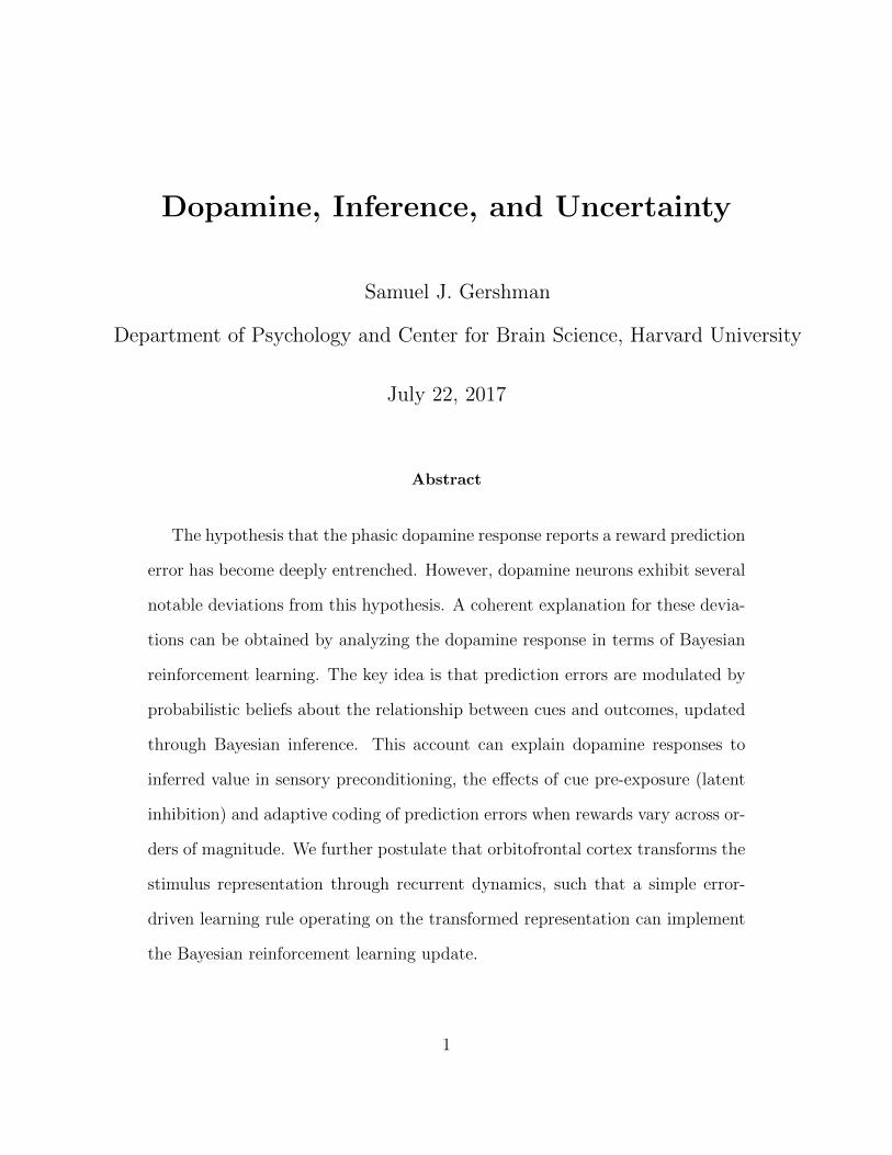
The hypothesis that the phasic dopamine response reports a reward prediction

error has become deeply entrenched. However, dopamine neurons exhibit several

notable deviations from this hypothesis. A coherent explanation for these devia-

tions can be obtained by analyzing the dopamine response in terms of Bayesian

reinforcement learning. The key idea is that prediction errors are modulated by

probabilistic beliefs about the relationship between cues and outcomes, updated

through Bayesian inference. This account can explain dopamine responses to

inferred value in sensory preconditioning, the effects of cue pre-exposure (latent

inhibition) and adaptive coding of prediction errors when rewards vary across or-

ders of magnitude. We further postulate that orbitofrontal cortex transforms the

stimulus representation through recurrent dynamics, such that a simple error-

driven learning rule operating on the transformed representation can implement

the Bayesian reinforcement learning update.

1

1 Introduction

The phasic firing of dopamine neurons in the midbrain has long been thought to report

a reward prediction error—the discrepancy between observed and expected reward—whose

purpose is to correct future reward predictions (Eshel et al., 2015; Glimcher, 2011; Montague

et al., 1996; Schultz et al., 1997). This hypothesis can explain many key properties of

dopamine, such as its sensitivity to the probability, magnitude and timing of reward, its

dynamics over the course of a trial, and its causal role in learning. Despite its success,

the prediction error hypothesis faces a number of puzzles. First, why do dopamine neurons

respond under some conditions, such as sensory preconditioning (Sadacca et al., 2016) and

latent inhibition (Young et al., 1993), where the prediction error should theoretically be

zero? Second, why do dopamine responses appear to rescale with the range or variance of

rewards (Tobler et al., 2005)? These phenomena appear to require a dramatic departure from

the normative foundations of reinforcement learning that originally motivated the prediction

error hypothesis (Sutton and Barto, 1998).

This paper provides a unified account of these phenomena, expanding the prediction error

hypothesis in a new direction while retaining its normative foundations. The first step is to

reconsider the computational problem being solved by the dopamine system: instead of com-

puting a single point estimate of expected future reward, the dopamine system recognizes its

own uncertainty by computing a probability distribution over expected future reward. This

probability distribution is updated dynamically using Bayesian inference, and the result-

ing learning equations retain the important features of earlier dopamine models. Crucially,

the Bayesian theory goes beyond earlier models by explaining why dopamine responses are

sensitive to sensory preconditioning, latent inhibition and reward variance.

The theory presented here was first developed to explain a broad range of associative learning

2

phenomena within a unifying framework (Gershman, 2015). We extend this theory further

by equipping it with a mechanism for updating beliefs about cue-specific volatility (i.e.,

how quickly associations between particular cues and outcomes change over time). This

mechanism harkens back to the classic Pearce-Hall theory of attention in associative learning

(Pearce and Hall, 1980; Pearce et al., 1982), as well as to more recent Bayesian incarnations

(Behrens et al., 2007; Mathys et al., 2011; Nassar et al., 2010; Yu and Dayan, 2005). As shown

below, volatility estimation is important for understanding the effect of reward variance on

the dopamine response.

2 Temporal difference learning

The prediction error hypothesis of dopamine was originally formalized by Montague et al.

(1996) in terms of the temporal difference (TD) learning algorithm (Sutton and Barto, 1998),

which posits an error signal of the form:

δt = rt + γVt+1 − Vt, (1)

where rt is the reward received at time t, γ ∈ [0, 1] is a discount factor that down-weights

distal rewards exponentially, and Vt is an estimate of the expected discounted future return

(or value):

Vt = E

[∑k=0

γkrt+k

]. (2)

By incrementally adjusting the parameters of the value function to minimize prediction er-

rors, TD learning gradually improves its estimates of future rewards. One common functional

form, both in machine learning and neurobiological applications, is linear function approxi-

3

mation, which approximates the value as a linear function of features xt: Vt = w>xt, where

w is a vector of weights, updated according to ∆w ∝ x>t δt.

In the complete serial compound (CSC) representation, each cue is broken down into a cas-

cade of temporal elements, such that each feature corresponds to a binary variable indicating

whether a stimulus is present or absent at a particular point in time. This allows the model to

generate temporally precise predictions, which have been systematically compared to phasic

dopamine signals. While the original work by Schultz et al. (1997) showed good agreement

between prediction errors and dopamine using the CSC, later work called into question its

adequacy (Daw et al., 2006; Gershman et al., 2014; Ludvig et al., 2008). Nonetheless, we

will adopt this representation for its simplicity, noting that our substantive conclusions are

unlikely to be changed with other temporal representations.

3 Reinforcement learning as Bayesian inference

The TD model is a point estimation algorithm, updating a single weight vector over time.

Gershman (2015) argued that associative learning is better modeled as Bayesian inference,

where a probability distribution over all possible weight vectors is updated over time. This

idea was originally explored by Dayan and colleagues (Dayan and Kakade, 2001; Dayan

et al., 2000) using a simple Bayesian extension of the Rescorla-Wagner model (the Kalman

filter). This model can explain retrospective revaluation phenomena like backward blocking

that posed notorious difficulties for classical models of associative learning (Miller et al.,

1995). Gershman (2015) illustrated the explanatory range of the Kalman filter by applying

it to numerous other phenomena. However, the Kalman filter is still fundamentally limited

by the fact that it is a trial-level model and hence cannot explain the effects of intra-trial

structure like the interstimulus interval or stimulus duration. It was precisely this structure

4

that motivated real-time frameworks like the TD model (Sutton and Barto, 1990).

The same logic that transforms Rescorla-Wagner into the Kalman filter can be applied to

transform the TD model into a Bayesian model (Geist and Pietquin, 2010). Gershman (2015)

showed how the resulting unified model (Kalman TD) can explain a range of phenomena

that neither the Kalman filter nor the TD model can explain in isolation. In this section, we

describe Kalman TD and its extension to incorporate volatility estimation. We then turn to

studies of the dopamine system, showing how the same model can provide a more complete

account of dopaminergic prediction errors.

3.1 Kalman temporal difference learning

To derive a Bayesian model, we first need to specify the data-generating process. In the

context of associative learning, this entails a prior probability distribution on the weight

vector, p(w0), a change process on the weights, p(wt|wt−1), and a reward distribution given

stimuli and weights, p(rt|wt,xt). Kalman TD assumes a linear-Gaussian dynamical system:

w0 ∼ N (0, σ2wI) (3)

wt ∼ N (wt−1,Q) (4)

rt ∼ N (w>t ht, σ2r), (5)

where I is the identity matrix, Q = diag(q1, . . . , qD) is a diagonal diffusion covariance matrix,

and ht = xt − γxt+1 is the discounted temporal derivative of the features. Intuitively, this

generative model assumes that weights change gradually and stochastically over time. Under

these assumptions, the value function can be expressed as a linear function of the features,

Vt = w>xt, just as in the linear function approximation architecture for TD (though in this

case the relationship is exact).

5

Given an observed sequence of feature vectors and rewards, Bayes’ rule stipulates how to

compute the posterior distribution over the weight vector:

p(wt|x1:t, r1:t) ∝ p(r1:t|wt,x1:t)p(wt). (6)

Under the generative assumptions described above, the Kalman filter can be used to update

the parameters of the posterior distribution in closed form. In particular, the posterior is

Gaussian with mean wt and covariance matrix Σt, updated according to:

wt+1 = wt + αtδt (7)

Σt+1 = Σt + Q− αtα>t

λt, (8)

where w0 = 0 is the initial weight vector (the prior mean), Σ0 = σ2wI is the initial (prior)

weight covariance matrix, αt = (Σt + Q)ht is a vector of learning rates, and

δt =δtλt

(9)

is the prediction error rescaled by the marginal variance

λt = h>t αt + σ2r , (10)

which encodes uncertainty about upcoming reward.

Like the original TD model, the Kalman TD model posits updating of weights by prediction

error, and the core empirical foundation of the TD model (see Glimcher, 2011) also applies to

Kalman TD. Unlike the original TD model, the learning rates change dynamically in Kalman

TD, a property important for explaining phenomena like latent inhibition, as discussed below.

In particular, learning rates increase with the posterior variance, reflecting the intuition

6

that new data should influence the posterior more when the agent is more uncertain. At

each timestep, the posterior variance increases due to unobserved stochastic changes in the

weights, but this increase may be compensated by reductions due to observed outcomes.

Another deviation from the original TD model is the fact that weight updates may not

be independent across cues; if there is non-zero covariance between cues, then observing

novel information about one cue will change beliefs about the other cue. This property is

instrumental to the explanation of various revaluation phenomena (Gershman, 2015), which

we explore below using the sensory preconditioning paradigm.

3.2 Volatility estimation

One unsatisfying, counterintuitive property of the Kalman TD model is that the learning

rates do not depend on the reward history. This means that the model will not be able to

capture changes in learning rate due to variability in the reward history. There is in fact

a considerable literature suggesting learning rate changes as a function of reward history,

though the precise nature of such changes is controversial (Le Pelley, 2004; Mitchell and

Le Pelley, 2010). For example, learning is slower when the cue was previously a reliable

predictor of reward (Hall and Pearce, 1979). Pearce and Hall (1980) interpreted this and

other findings as evidence that learning rate declines with cue-outcome reliability. They

formalized this idea by assuming that learning rate is proportional to the absolute prediction

error (see Roesch et al., 2012, for a review of the behavioral and neural evidence).

A similar mechanism can be derived from first principles within the Kalman TD framework.

We have so far assumed that the diffusion covariance matrix Q is known, but the diagonal

elements (diffusion variances) q1, . . . , qD can be estimated by maximum likelihood methods.

In particular, we can derive a stochastic gradient descent rule by differentiating the log-

7

likelihood with respect to the diffusion variances:

∆qd = ηh2tdδ2t − 1

λt, (11)

where η is a learning rate. This update rule exhibits the desired dependence of learning rate

on the unsigned prediction error (δ2), since learning rate for cue d increases monotonically

with qd.

3.3 Modeling details

We use the same parameters as in our earlier paper (Gershman, 2015): σ2w = 1, σ2

r = 1,

and γ = 0.98. The volatilities were initialized to qd = 0.01 and then updated using a meta-

learning rate of η = 0.1. Stimuli were modeled with a 4-time-step CSC representation and

an intertrial interval of 6 time-steps.

4 Applications to the dopamine system

We are now in a position to resolve the puzzles with which we started, focusing on two

empirical implications of the TD model. First, the model only updates the weights of present

cues, and hence cues that have not been paired directly with reward or with reward-predicting

cues should not elicit a dopamine response. This implication disagrees with findings from

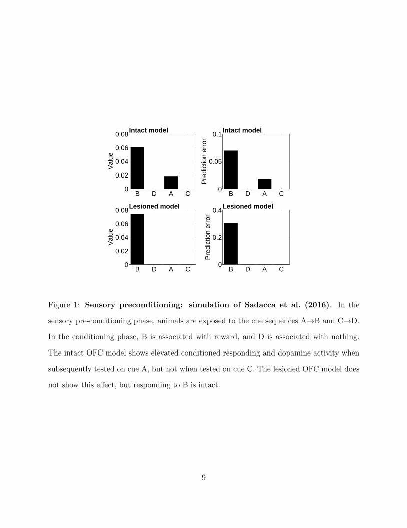
a sensory preconditioning procedure (Sadacca et al., 2016), where cue A is sequentially

paired with cue B and cue C is sequentially paired with cue D (Figure 1). If cue B is

subsequently paired with reward and cue D is paired with nothing, cue A comes to elicit

both a conditioned response and elevated dopamine activity compared to cue B. The TD

model predicts no dopamine response to either A or B. The Kalman TD model, in contrast,

8

B D A C0

0.02

0.04

0.06

0.08

Val

ue

Intact model

B D A C0

0.05

0.1

Pre

dict

ion

erro

r

Intact model

B D A C0

0.02

0.04

0.06

0.08

Val

ue

Lesioned model

B D A C0

0.2

0.4P

redi

ctio

n er

ror

Lesioned model

Figure 1: Sensory preconditioning: simulation of Sadacca et al. (2016). In the

sensory pre-conditioning phase, animals are exposed to the cue sequences A→B and C→D.

In the conditioning phase, B is associated with reward, and D is associated with nothing.

The intact OFC model shows elevated conditioned responding and dopamine activity when

subsequently tested on cue A, but not when tested on cue C. The lesioned OFC model does

not show this effect, but responding to B is intact.

9

1 2 3 4 50

0.02

0.04

0.06

0.08

0.1

0.12

Pre

dict

ion

erro

r

Trial

PreNoPre

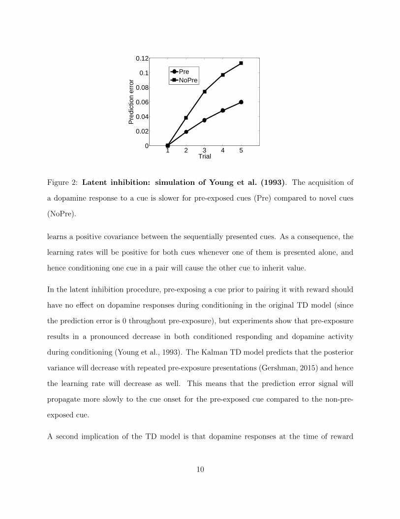
Figure 2: Latent inhibition: simulation of Young et al. (1993). The acquisition of

a dopamine response to a cue is slower for pre-exposed cues (Pre) compared to novel cues

(NoPre).

learns a positive covariance between the sequentially presented cues. As a consequence, the

learning rates will be positive for both cues whenever one of them is presented alone, and

hence conditioning one cue in a pair will cause the other cue to inherit value.

In the latent inhibition procedure, pre-exposing a cue prior to pairing it with reward should

have no effect on dopamine responses during conditioning in the original TD model (since

the prediction error is 0 throughout pre-exposure), but experiments show that pre-exposure

results in a pronounced decrease in both conditioned responding and dopamine activity

during conditioning (Young et al., 1993). The Kalman TD model predicts that the posterior

variance will decrease with repeated pre-exposure presentations (Gershman, 2015) and hence

the learning rate will decrease as well. This means that the prediction error signal will

propagate more slowly to the cue onset for the pre-exposed cue compared to the non-pre-

exposed cue.

A second implication of the TD model is that dopamine responses at the time of reward

10

should scale with reward magnitude. This implication disagrees with the work of (Tobler

et al., 2005), who paired different cues half the time with a cue-specific reward magnitude

(liquid volume) and half the time with no reward. Although dopamine neurons increased

their firing rate whenever reward was delivered, the size of this increase was essentially un-

changed across cues despite the reward magnitudes varying over an order of magnitude.

Tobler et al. (2005) interpreted this finding as evidence for a form of “adaptive coding,”

whereby dopamine neurons adjust their dynamic range to accommodate different distribu-

tions of prediction errors (see also Diederen and Schultz, 2015; Diederen et al., 2016, for

converging evidence from humans). Adaptive coding has been found throughout sensory ar-

eas as well as in reward-processing areas (Louie and Glimcher, 2012). While adaptive coding

can be motivated by information-theoretic arguments (Atick, 1992), the question is how to

reconcile this property with the TD model.

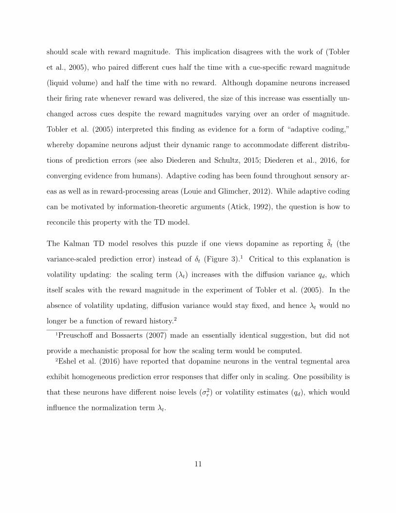
The Kalman TD model resolves this puzzle if one views dopamine as reporting δt (the

variance-scaled prediction error) instead of δt (Figure 3).1 Critical to this explanation is

volatility updating: the scaling term (λt) increases with the diffusion variance qd, which

itself scales with the reward magnitude in the experiment of Tobler et al. (2005). In the

absence of volatility updating, diffusion variance would stay fixed, and hence λt would no

longer be a function of reward history.2

1Preuschoff and Bossaerts (2007) made an essentially identical suggestion, but did not

provide a mechanistic proposal for how the scaling term would be computed.2Eshel et al. (2016) have reported that dopamine neurons in the ventral tegmental area

exhibit homogeneous prediction error responses that differ only in scaling. One possibility is

that these neurons have different noise levels (σ2r) or volatility estimates (qd), which would

influence the normalization term λt.

11

2 4 6 8 100

2

4

6

8

10

Pre

dict

ion

erro

r

Reward magnitude

NormalizedUnnormalized

Figure 3: Adaptive coding: simulation of Tobler et al. (2005). Each cue is associated

with a 50% chance of earning a fixed reward, and 50% chance of nothing. Dopamine neu-

rons show increased responding to the reward compared to nothing, but this increase does

not change across cues delivering different amounts of reward. This finding is inconsistent

with the standard TD prediction error account, but is consistent with the hypothesis that

prediction errors are divided by the posterior predictive variance.

12

5 Representational transformation in the orbitofrontal

cortex

Dayan and Kakade (2001) described a neural circuit that approximates the Kalman filter, but

did not explore its empirical implications. This section reconsiders the circuit implementation

applied to the Kalman TD model, and then discusses experimental data relevant to its neural

substrate.

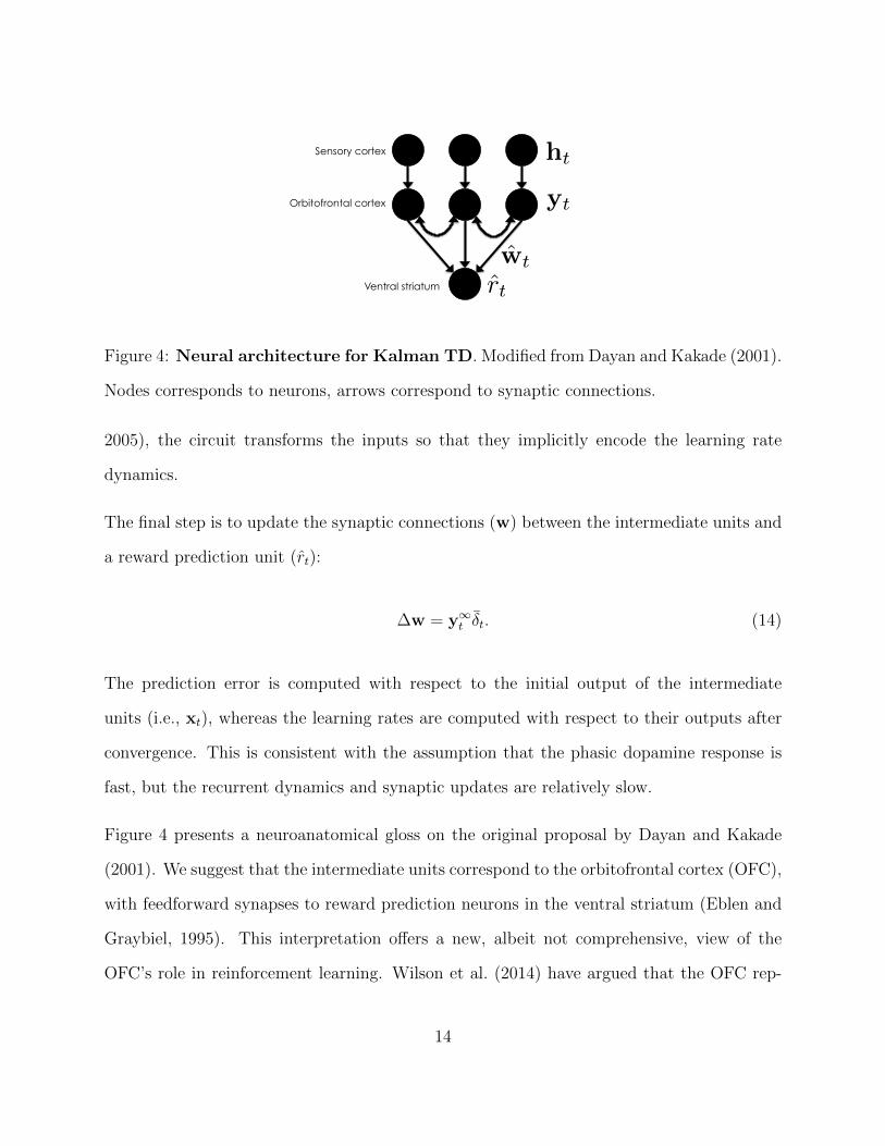
The network architecture is shown in Figure 4. The input units represent the discounted fea-

ture derivatives, ht, which are then passed through an identity mapping to the intermediate

units yt. The intermediate units are recurrently connected with a synaptic weight matrix B

and undergo linear dynamics given by:

τ yt = −yt + ht + Byt, (12)

where τ is a time constant. These dynamics will converge to y∞t = (I−B)−1ht, assuming the

inverse exists. The synaptic weight matrix is updated according to an anti-Hebbian learning

rule (Atick and Redlich, 1993; Goodall, 1960):

∆B ∝ −hty>t + I−B. (13)

If B is initialized to all zeros, this learning rule asymptotically satisfies (I−B)−1 = E[Σt]. It

follows that y∞t = E[αt] asymptotically. Thus, the intermediate units, in the limit of infinite

past experience and infinite computation time, approximate the learning rates required by

the Kalman filter. As noted by Dayan and Kakade (2001), the resulting outputs can be

viewed as decorrelated (whitened) versions of the inputs. Instead of modulating learning

rates over time (e.g., using neuromodulation; Doya, 2002; Nassar et al., 2012; Yu and Dayan,

13

ht

yt

wt

rt

Sensory cortex

Orbitofrontal cortex

Ventral striatum

Figure 4: Neural architecture for Kalman TD. Modified from Dayan and Kakade (2001).

Nodes corresponds to neurons, arrows correspond to synaptic connections.

2005), the circuit transforms the inputs so that they implicitly encode the learning rate

dynamics.

The final step is to update the synaptic connections (w) between the intermediate units and

a reward prediction unit (rt):

∆w = y∞t δt. (14)

The prediction error is computed with respect to the initial output of the intermediate

units (i.e., xt), whereas the learning rates are computed with respect to their outputs after

convergence. This is consistent with the assumption that the phasic dopamine response is

fast, but the recurrent dynamics and synaptic updates are relatively slow.

Figure 4 presents a neuroanatomical gloss on the original proposal by Dayan and Kakade

(2001). We suggest that the intermediate units correspond to the orbitofrontal cortex (OFC),

with feedforward synapses to reward prediction neurons in the ventral striatum (Eblen and

Graybiel, 1995). This interpretation offers a new, albeit not comprehensive, view of the

OFC’s role in reinforcement learning. Wilson et al. (2014) have argued that the OFC rep-

14

resents a “cognitive map” of task space, providing the state representation over which TD

learning operates. The circuit described above can be viewed as implementing one form of

state representation based on a whitening transform.

If this interpretation is correct, then OFC damage should be devastating for some kinds

of associative learning (namely, those that entail non-zero covariance between cues) while

leaving other kinds of learning intact (namely, those that entail uncorrelated cues). A par-

ticularly useful example of this dissociation comes from work by Jones et al. (2012), which

demonstrated that OFC lesions eliminate sensory preconditioning while leaving first-order

conditioning intact. This pattern is reproduced by the Kalman TD model if the intermedi-

ate units are “lesioned” such that no input transformation occurs (i.e., inputs are mapped

directly to rewards; Figure 1). In other words, the lesioned model is reduced to the original

TD model with fixed learning rates.

6 Discussion

The twin roles of Bayesian inference and reinforcement learning have a long history in animal

learning theory, but until recently these ideas were not unified into a single theory known

as Kalman TD (Gershman, 2015). In this paper, we applied the theory to several puz-

zling phenomena in the dopamine system: the sensitivity of dopamine neurons to posterior

variance (latent inhibition), covariance (sensory preconditioning) and posterior predictive

variance (adaptive coding). These phenomena could be explained by making two principled

modifications to the prediction error hypothesis of dopamine. First, the learning rate, which

drives updating of values, is vector-valued in Kalman TD, with the result that associative

weights for cues can be updated even when that cue is not present, provided it has non-zero

covariance with another cue. Furthermore, the learning rates can change over time, modu-

15

lated by the agent’s uncertainty. Second, Kalman TD posits that dopamine neurons report

a normalized prediction error, δt, such that greater uncertainty suppresses dopamine activity

(see also Preuschoff and Bossaerts, 2007).

How are the probabilistic computations of Kalman TD implemented in the brain? We

modified the proposal of Dayan and Kakade (2001), according to which recurrent dynam-

ics produce a transformation of the stimulus inputs that effectively whitens (decorrelates)

them. Standard error-driven learning rules operating on the decorrelated input are then

mathematically equivalent to the Kalman TD updates. One potential neural substrate for

this stimulus transformation is the OFC, a critical hub for state representation in RL (Wilson

et al., 2014). We showed that lesioning the OFC forces the network to fall back on a stan-

dard TD update (i.e., ignoring the covariance structure). This prevents the network from

exhibiting sensory preconditioning, as has been observed experimentally (Jones et al., 2012).

The idea that recurrent dynamics in OFC play an important role in stimulus representation

for reinforcement learning and reward expectation has also figured in earlier models (Deco

and Rolls, 2005; Frank and Claus, 2006).

Kalman TD is closely related to the hypothesis that dopaminergic prediction errors operate

over belief state representations. These representations arise when an agent has uncertainty

about the hidden state of the world. Bayes’ rule prescribes that this uncertainty be rep-

resented as a posterior distribution over states (the belief state), which can then feed into

standard TD learning mechanisms. Several authors have proposed that belief states could

explain some anomalous patterns of dopamine responses (Daw et al., 2006; Rao, 2010), and

experimental evidence has recently accumulated for this proposal (Lak et al., 2017; Stark-

weather et al., 2017; Takahashi et al., 2016). One way to understand Kalman TD is to think

of the weight vector as part of the hidden state. A similar conceptual move has been stud-

ied in computer science, in which the parameters of a Markov decision process are treated

16

as unknown, thereby transforming it into a partially observable Markov decision process

(Duff, 2002; Poupart et al., 2006). Kalman TD is a model-free counterpart to this idea,

treating the parameters of the function approximator as unknown. This view allows one to

contemplate more complex versions of the model proposed here, for example with nonlinear

function approximators or structure learning (Gershman et al., 2015), although inference

quickly becomes intractable in these cases.

A number of other authors have suggested that dopamine responses are related to Bayesian

inference in various ways. Friston and colleagues have developed a theory grounded in a vari-

ational approximation of Bayesian inference, whereby phasic dopamine reports changes in

the estimate of inverse variance (FitzGerald et al., 2015; Friston et al., 2012; Schwartenbeck

et al., 2014). This theory fits well with the modulatory effects of dopamine on downstream

circuits, but it is currently unclear to what extent this theoretical framework can account for

the body of empirical data on which the prediction error hypothesis of dopamine is based.

Other authors have suggested that dopamine is involved in specifying a prior probability

distribution (Costa et al., 2015) or influencing uncertainty representation in the striatum

(Mikhael and Bogacz, 2016). These different possibilities are not necessarily mutually exclu-

sive, but more research is necessary to bridge these varied roles of dopamine in probabilistic

computation.

Of particular relevance here is the finding that sustained dopamine activation during the

interstimulus interval of a Pavlovian conditioning task appears to code reward uncertainty,

with maximal activation to cues that are the least reliable predictors of upcoming reward

(Fiorillo et al., 2003). Although it has been argued that this finding may be an averaging

artifact (Niv et al., 2005), subsequent research has confirmed that uncertainty coding is a

distinct signal (Hart et al., 2015). This suggests that dopamine may convey multiple signals,

only some of which can be explained in terms of prediction errors as pursued here.

17

The Kalman TD model makes several new experimental predictions. First, it predicts that

a host of post-training manipulations, identified as problematic for traditional associative

learning (Gershman, 2015; Miller et al., 1995), should have systematic effects on dopamine

responses. For example, extinguishing the blocking cue in a blocking paradigm causes recov-

ery of responding to the blocked cue in a subsequent test (Blaisdell et al., 1999); the Kalman

TD model predicts that this extinction procedure should cause a positive dopaminergic re-

sponse to the blocked cue. Note that this prediction does not follow from the probabilistic

interpretation of dopamine in terms of changes in inverse variance (FitzGerald et al., 2015;

Friston et al., 2012; Schwartenbeck et al., 2014), which reflects beliefs about policies (whereas

we have restricted our attention to Pavlovian state values). A second prediction is that the

OFC should exhibit dynamic cue competition and facilitation (depending on the paradigm).

For example, in the sensory preconditioning paradigm (where facilitation prevails), neurons

selective for one cue should be correlated with the neurons selective for another cue, such that

presenting one cue will activate neurons selective for the other cue. By contrast, in a back-

ward blocking paradigm (where competition prevails), neurons selective for different cues

should be anti-correlated. Finally, OFC lesions in these same paradigms should eliminate

the sensitivity of dopamine neurons to post-training manipulations.

One general limitation of Kalman TD is that it imposes strenuous computational costs: for

D stimulus dimensions, a D ×D covariance matrix must be maintained and updated. This

representation thus does not scale well to high-dimensional spaces, but there are a number of

ways the cost can be reduced. In many real-world domains, the intrinsic dimensionality of the

state space is lower than the dimensionality of the ambient stimulus space. This suggests that

a dimensionality reduction step could be combined with Kalman TD so that the covariance

matrix is defined over a low-dimensional state space. Several lines of evidence suggest that

this is indeed what the brain does. First, cortical inputs into the striatum are massively

convergent, with an order of magnitude reduction in the number of neurons from cortex to

18

striatum (Zheng and Wilson, 2002). Bar-Gad et al. (2003) have argued that this anatomical

organization is well-suited for reinforcement-driven dimensionality reduction. Second, the

evidence that dopamine reward prediction errors exhibit signatures of belief states (Lak

et al., 2017; Starkweather et al., 2017; Takahashi et al., 2016) is consistent with the view

that value functions are defined over low-dimensional hidden states. Third, there are many

behavioral phenomena that suggest animals are learning about hidden states (Courville

et al., 2006; Gershman et al., 2015). Computational models of hidden state inference could

be productively combined with Kalman TD in future work.

The theory presented here does not pretend to be a complete account of dopamine; there

remain numerous anomalies that will keep RL theorists busy for a long time (Dayan and

Niv, 2008). The contribution of this work is to chart a new avenue for thinking about the

function of dopamine in probabilistic terms, with the aim of building a bridge between RL

and Bayesian approaches to learning in the brain.

Acknowledgments

This research was supported by the NSF Collaborative Research in Computational Neuro-

science (CRCNS) Program Grant IIS-120 7833.

References

Atick, J. J. (1992). Could information theory provide an ecological theory of sensory pro-

cessing? Network: Computation in neural systems, 3:213–251.

Atick, J. J. and Redlich, A. N. (1993). Convergent algorithm for sensory receptive field

development. Neural Computation, 5:45–60.

19

Bar-Gad, I., Morris, G., and Bergman, H. (2003). Information processing, dimensionality

reduction and reinforcement learning in the basal ganglia. Progress in Neurobiology,

71:439–473.

Behrens, T. E., Woolrich, M. W., Walton, M. E., and Rushworth, M. F. (2007). Learning

the value of information in an uncertain world. Nature Neuroscience, 10:1214–1221.

Blaisdell, A. P., Gunther, L. M., and Miller, R. R. (1999). Recovery from blocking achieved

by extinguishing the blocking CS. Animal Learning & Behavior, 27:63–76.

Costa, V. D., Tran, V. L., Turchi, J., and Averbeck, B. B. (2015). Reversal learning and

dopamine: a Bayesian perspective. Journal of Neuroscience, 35:2407–2416.

Courville, A. C., Daw, N. D., and Touretzky, D. S. (2006). Bayesian theories of conditioning

in a changing world. Trends in Cognitive Sciences, 10:294–300.

Daw, N. D., Courville, A. C., and Touretzky, D. S. (2006). Representation and timing in

theories of the dopamine system. Neural Computation, 18:1637–1677.

Dayan, P. and Kakade, S. (2001). Explaining away in weight space. In Leen, T., Dietterich,

T., and Tresp, V., editors, Advances in Neural Information Processing Systems 13,

pages 451–457. MIT Press.

Dayan, P., Kakade, S., and Montague, P. R. (2000). Learning and selective attention. Nature

Neuroscience, 3:1218–1223.

Dayan, P. and Niv, Y. (2008). Reinforcement learning: the good, the bad and the ugly.

Current Opinion in Neurobiology, 18:185–196.

Deco, G. and Rolls, E. T. (2005). Synaptic and spiking dynamics underlying reward reversal

in the orbitofrontal cortex. Cerebral Cortex, 15:15–30.

Diederen, K. M. and Schultz, W. (2015). Scaling prediction errors to reward variability

benefits error-driven learning in humans. Journal of Neurophysiology, 114:1628–1640.

Diederen, K. M., Spencer, T., Vestergaard, M. D., Fletcher, P. C., and Schultz, W. (2016).

Adaptive prediction error coding in the human midbrain and striatum facilitates be-

20

havioral adaptation and learning efficiency. Neuron, 90:1127–1138.

Doya, K. (2002). Metalearning and neuromodulation. Neural Networks, 15:495–506.

Duff, M. O. (2002). Optimal Learning: Computational procedures for Bayes-adaptive Markov

decision processes. PhD thesis, University of Massachusetts Amherst.

Eblen, F. and Graybiel, A. M. (1995). Highly restricted origin of prefrontal cortical inputs

to striosomes in the macaque monkey. Journal of Neuroscience, 15:5999–6013.

Eshel, N., Bukwich, M., Rao, V., Hemmelder, V., Tian, J., and Uchida, N. (2015). Arithmetic

and local circuitry underlying dopamine prediction errors. Nature, 525:243–246.

Eshel, N., Tian, J., Bukwich, M., and Uchida, N. (2016). Dopamine neurons share common

response function for reward prediction error. Nature Neuroscience, 19:479–486.

Fiorillo, C. D., Tobler, P. N., and Schultz, W. (2003). Discrete coding of reward probability

and uncertainty by dopamine neurons. Science, 299:1898–1902.

FitzGerald, T. H., Dolan, R. J., and Friston, K. (2015). Dopamine, reward learning, and

active inference. Frontiers in Computational Neuroscience, 9.

Frank, M. J. and Claus, E. D. (2006). Anatomy of a decision: striato-orbitofrontal interac-

tions in reinforcement learning, decision making, and reversal. Psychological Review,

113:300–326.

Friston, K. J., Shiner, T., FitzGerald, T., Galea, J. M., Adams, R., Brown, H., Dolan, R. J.,

Moran, R., Stephan, K. E., and Bestmann, S. (2012). Dopamine, affordance and active

inference. PLoS Computational Biology, 8:e1002327.

Geist, M. and Pietquin, O. (2010). Kalman temporal differences. Journal of Artificial

Intelligence Research, 39:483–532.

Gershman, S. J. (2015). A unifying probabilistic view of associative learning. PLoS Compu-

tational Biology, 11:e1004567.

Gershman, S. J., Moustafa, A. A., and Ludvig, E. A. (2014). Time representation in reinforce-

ment learning models of the basal ganglia. Frontiers in Computational Neuroscience,

21

7.

Gershman, S. J., Norman, K. A., and Niv, Y. (2015). Discovering latent causes in reinforce-

ment learning. Current Opinion in Behavioral Sciences, 5:43–50.

Glimcher, P. W. (2011). Understanding dopamine and reinforcement learning: the dopamine

reward prediction error hypothesis. Proceedings of the National Academy of Sciences,

108(Supplement 3):15647–15654.

Goodall, M. (1960). Performance of a stochastic net. Nature, 185:557–558.

Hall, G. and Pearce, J. M. (1979). Latent inhibition of a CS during CS-US pairings. Journal

of Experimental Psychology: Animal Behavior Processes, 5:31–42.

Hart, A. S., Clark, J. J., and Phillips, P. E. (2015). Dynamic shaping of dopamine signals

during probabilistic Pavlovian conditioning. Neurobiology of Learning and Memory,

117:84–92.

Jones, J. L., Esber, G. R., McDannald, M. A., Gruber, A. J., Hernandez, A., Mirenzi, A.,

and Schoenbaum, G. (2012). Orbitofrontal cortex supports behavior and learning using

inferred but not cached values. Science, 338:953–956.

Lak, A., Nomoto, K., Keramati, M., Sakagami, M., and Kepecs, A. (2017). Midbrain

dopamine neurons signal belief in choice accuracy during a perceptual decision. Current

Biology, 27:821–832.

Le Pelley, M. E. (2004). The role of associative history in models of associative learning:

A selective review and a hybrid model. Quarterly Journal of Experimental Psychology

Section B, 57:193–243.

Louie, K. and Glimcher, P. W. (2012). Efficient coding and the neural representation of

value. Annals of the New York Academy of Sciences, 1251:13–32.

Ludvig, E. A., Sutton, R. S., and Kehoe, E. J. (2008). Stimulus representation and the timing

of reward-prediction errors in models of the dopamine system. Neural Computation,

20:3034–3054.

22

Mathys, C., Daunizeau, J., Friston, K. J., and Stephan, K. E. (2011). A Bayesian foundation

for individual learning under uncertainty. Frontiers in Human Neuroscience, 5.

Mikhael, J. G. and Bogacz, R. (2016). Learning reward uncertainty in the basal ganglia.

PLoS Computational Biology, 12:e1005062.

Miller, R. R., Barnet, R. C., and Grahame, N. J. (1995). Assessment of the Rescorla-Wagner

model. Psychological Bulletin, 117:363–386.

Mitchell, C. J. and Le Pelley, M. E. (2010). Attention and Associative Learning: From Brain

to Behaviour. Oxford University Press, USA.

Montague, P. R., Dayan, P., and Sejnowski, T. J. (1996). A framework for mesencephalic

dopamine systems based on predictive Hebbian learning. Journal of Neuroscience,

16:1936–1947.

Nassar, M. R., Rumsey, K. M., Wilson, R. C., Parikh, K., Heasly, B., and Gold, J. I.

(2012). Rational regulation of learning dynamics by pupil-linked arousal systems.

Nature Neuroscience, 15:1040–1046.

Nassar, M. R., Wilson, R. C., Heasly, B., and Gold, J. I. (2010). An approximately bayesian

delta-rule model explains the dynamics of belief updating in a changing environment.

The Journal of Neuroscience, 30:12366–12378.

Niv, Y., Duff, M. O., and Dayan, P. (2005). Dopamine, uncertainty and TD learning.

Behavioral and Brain Functions, 1:1–6.

Pearce, J. and Hall, G. (1980). A model for Pavlovian learning: Variations in the effectiveness

of conditioned but not of unconditioned stimuli. Psychological Review, 87:532–552.

Pearce, J., Kaye, H., and Hall, G. (1982). Predictive accuracy and stimulus associability:

Development of a model for Pavlovian learning. Quantitative analyses of behavior,

3:241–255.

Poupart, P., Vlassis, N., Hoey, J., and Regan, K. (2006). An analytic solution to discrete

Bayesian reinforcement learning. In Proceedings of the 23rd international conference

23

on Machine learning, pages 697–704. ACM.

Preuschoff, K. and Bossaerts, P. (2007). Adding prediction risk to the theory of reward

learning. Annals of the New York Academy of Sciences, 1104:135–146.

Rao, R. P. (2010). Decision making under uncertainty: a neural model based on partially

observable Markov decision processes. Frontiers in Computational Neuroscience, 4:146.

Roesch, M. R., Esber, G. R., Li, J., Daw, N. D., and Schoenbaum, G. (2012). Surprise!

neural correlates of pearce–hall and rescorla–wagner coexist within the brain. European

Journal of Neuroscience, 35:1190–1200.

Sadacca, B. F., Jones, J. L., and Schoenbaum, G. (2016). Midbrain dopamine neurons

compute inferred and cached value prediction errors in a common framework. Elife,

5:e13665.

Schultz, W., Dayan, P., and Montague, P. R. (1997). A neural substrate of prediction and

reward. Science, 275:1593–1599.

Schwartenbeck, P., FitzGerald, T. H., Mathys, C., Dolan, R., and Friston, K. (2014). The

dopaminergic midbrain encodes the expected certainty about desired outcomes. Cere-

bral Cortex, 25::3434–3445.

Starkweather, C. K., Babayan, B. M., Uchida, N., and Gershman, S. J. (2017). Dopamine re-

ward prediction errors reflect hidden-state inference across time. Nature Neuroscience,

20:581–589.

Sutton, R. and Barto, A. (1990). Time-derivative models of pavlovian reinforcement. In

Gabriel, M. and Moore, J., editors, Learning and Computational Neuroscience: Foun-

dations of Adaptive Networks, pages 497–537. MIT Press.

Sutton, R. S. and Barto, A. G. (1998). Reinforcement Learning: An Introduction. MIT

Press.

Takahashi, Y. K., Langdon, A. J., Niv, Y., and Schoenbaum, G. (2016). Temporal specificity

of reward prediction errors signaled by putative dopamine neurons in rat VTA depends

24

on ventral striatum. Neuron, 91:182–193.

Tobler, P. N., Fiorillo, C. D., and Schultz, W. (2005). Adaptive coding of reward value by

dopamine neurons. Science, 307:1642–1645.

Wilson, R. C., Takahashi, Y. K., Schoenbaum, G., and Niv, Y. (2014). Orbitofrontal cortex

as a cognitive map of task space. Neuron, 81:267–279.

Young, A., Joseph, M., and Gray, J. (1993). Latent inhibition of conditioned dopamine

release in rat nucleus accumbens. Neuroscience, 54:5–9.

Yu, A. J. and Dayan, P. (2005). Uncertainty, neuromodulation, and attention. Neuron,

46:681–692.

Zheng, T. and Wilson, C. (2002). Corticostriatal combinatorics: the implications of corti-

costriatal axonal arborizations. Journal of Neurophysiology, 87:1007–1017.

25