Embed Size (px)
Citation preview

Domain Flow
Dr. E. Theodore L. Omtzigt
Re-emergence of data flow
March 2008
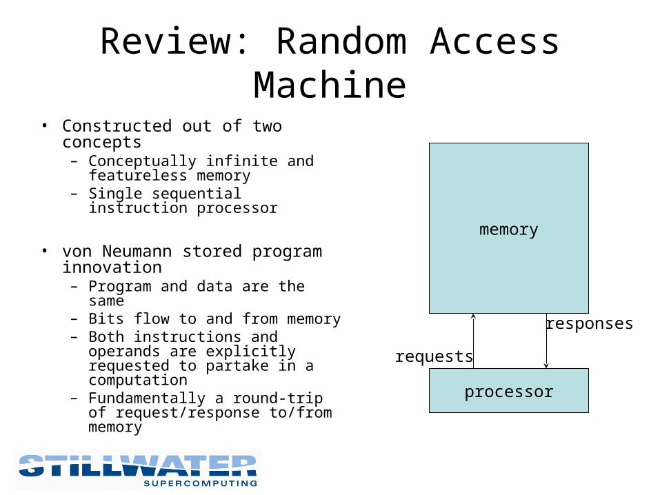
Review: Random Access Machine
• Constructed out of two concepts– Conceptually infinite and
featureless memory– Single sequential instruction
processor
• von Neumann stored program innovation– Program and data are the same– Bits flow to and from memory– Both instructions and operands
are explicitly requested to partake in a computation
– Fundamentally a round-trip of request/response to/from memory
memory
processor
requests
responses
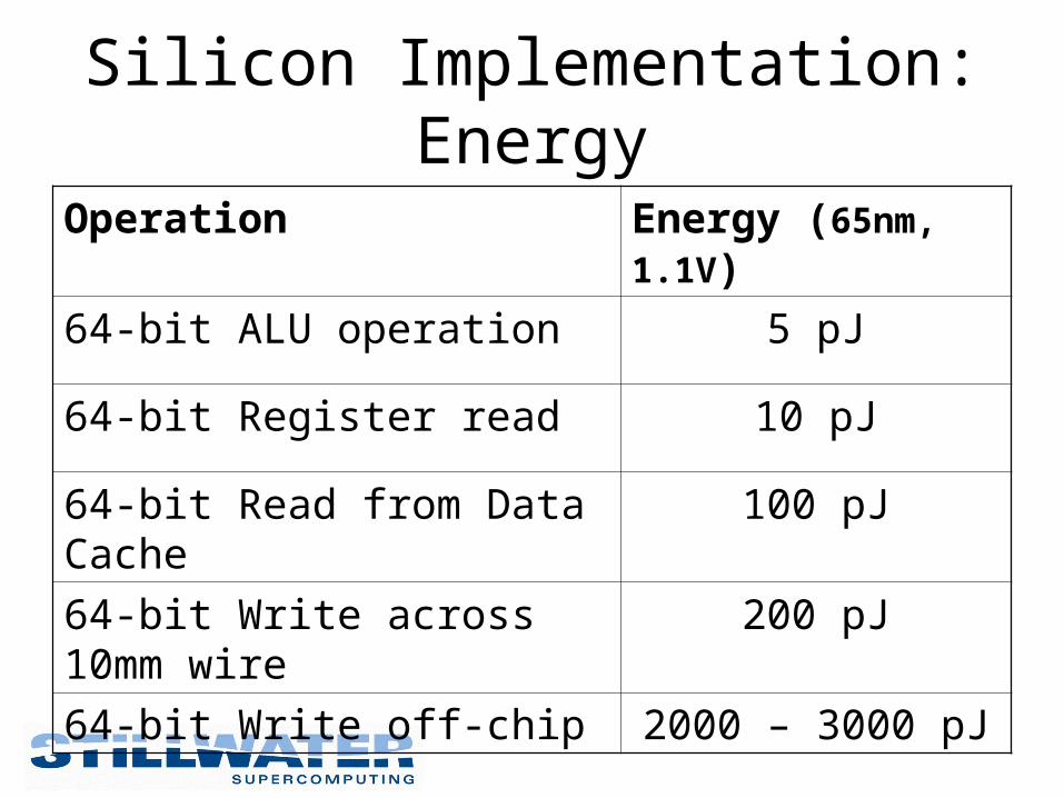
Silicon Implementation: Energy
Operation Energy (65nm, 1.1V)
64-bit ALU operation 5 pJ
64-bit Register read 10 pJ
64-bit Read from Data Cache 100 pJ
64-bit Write across 10mm wire
200 pJ
64-bit Write off-chip 2000 – 3000 pJ
Sequential vs Parallel Execution
• Sequential Execution– Request/reply cycle to flat memory– Large overhead to provision an operator
• fetch, decode, schedule, execute, write
– Not very energy efficient• Control uses 30 times the energy of a 64-bit MAC
– Can’t take advantage of structure
• Parallel Execution– Concurrent data movement
• No need for request/response cycles
– Can bake structure of the algorithm in the control strategy!• Order of magnitude better efficiency
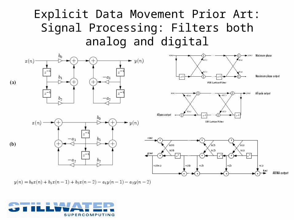
Explicit Data Movement Prior Art:Signal Processing: Filters both analog and digital

Explicit Data Movement Prior Art:Signal Processing: Amplifiers, conditioners, drivers, etc.

Signal Flow Graphs

Data Flow Graphs
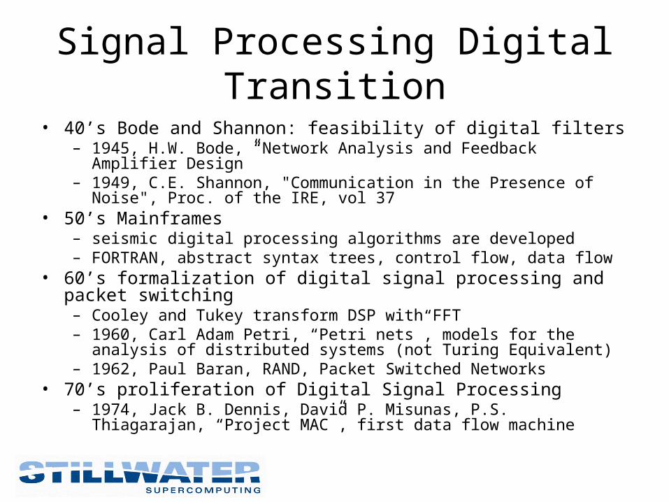
Signal Processing Digital Transition
• 40’s Bode and Shannon: feasibility of digital filters– 1945, H.W. Bode, “Network Analysis and Feedback Amplifier Design”– 1949, C.E. Shannon, "Communication in the Presence of Noise", Proc.
of the IRE, vol 37• 50’s Mainframes
– seismic digital processing algorithms are developed– FORTRAN, abstract syntax trees, control flow, data flow
• 60’s formalization of digital signal processing and packet switching– Cooley and Tukey transform DSP with FFT– 1960, Carl Adam Petri, “Petri nets”, models for the analysis of
distributed systems (not Turing Equivalent)– 1962, Paul Baran, RAND, Packet Switched Networks
• 70’s proliferation of Digital Signal Processing– 1974, Jack B. Dennis, David P. Misunas, P.S. Thiagarajan, “Project
MAC”, first data flow machine
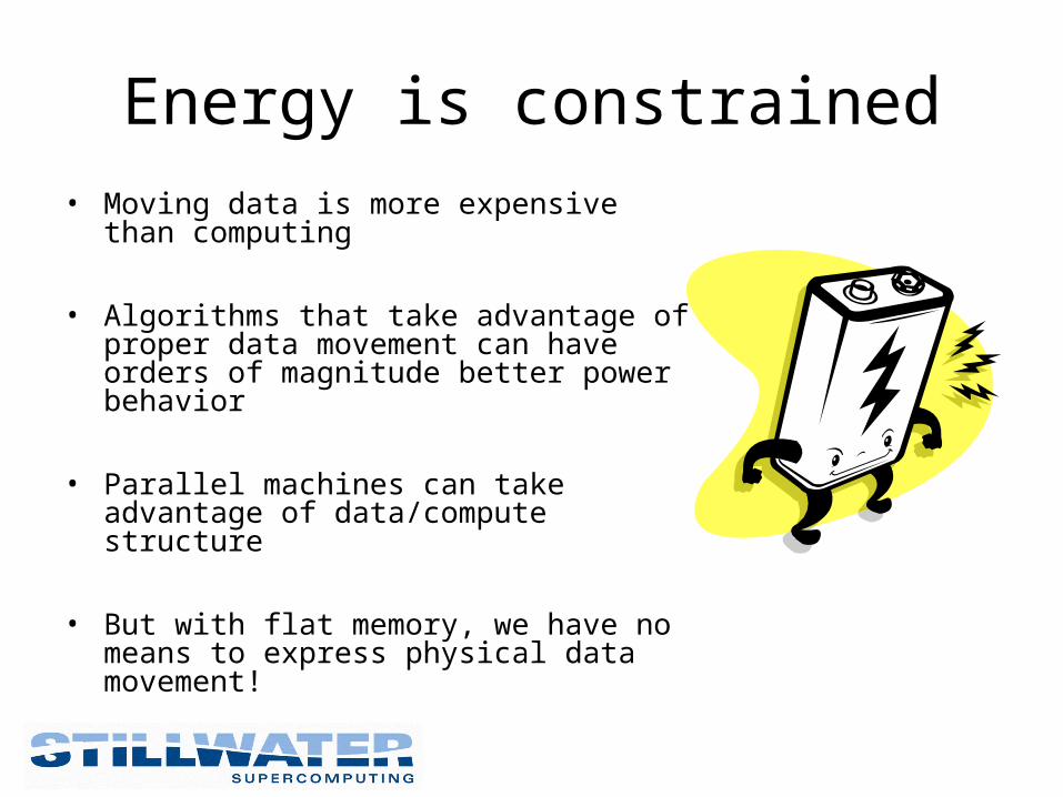
Energy is constrained• Moving data is more expensive than
computing
• Algorithms that take advantage of proper data movement can have orders of magnitude better power behavior
• Parallel machines can take advantage of data/compute structure
• But with flat memory, we have no means to express physical data movement!

Computational Space-time• Space-time affects structure of optimal algorithms
– Flat memory does not exist• GAS does not help writing energy efficient algorithms
– Architecture needs to quantify time and distance• Simplify architecture to allow software to be more efficient
• Space-time normalizes distance to time– Perfect for making communication delays explicit– Distance is proportional to energy spent– Minimizing data movement minimizes energy and is good for performance
• Introduce new programming model– Computational space-time captures distance/delay attributes of a machine– Cones of influence are the parts of the machine you can affect in one unit of time
• One unit of time is equal to the fundamental operation in the SFG/DFG• Think lattice filters

Cones of influence
Processor world line

Scalable Architecture• Chip process technology scaling
– Transistor and wire delays scale differently
• Uniform Architecture– Constant computation/communication
delays– Constant compute/communication
balance– Algorithm dynamics stay constant
• Scale down in process technology– Higher speed, lower power, lower cost
• Scale up in size: high throughput
• 3D/4D Orthonormal lattices– Represent uniform architecture– Design once, run optimally for ever– No need for retuning between processor
generations
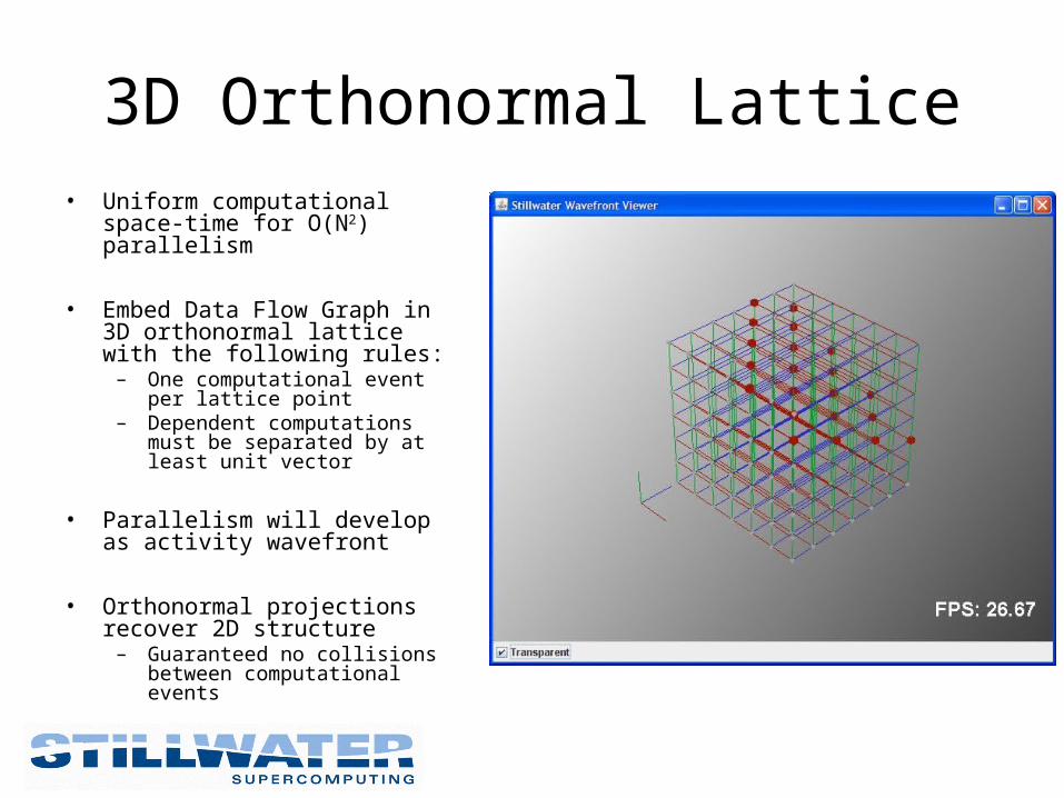
3D Orthonormal Lattice• Uniform computational space-time
for O(N2) parallelism
• Embed Data Flow Graph in 3D orthonormal lattice with the following rules:
– One computational event per lattice point
– Dependent computations must be separated by at least unit vector
• Parallelism will develop as activity wavefront
• Orthonormal projections recover 2D structure
– Guaranteed no collisions between computational events
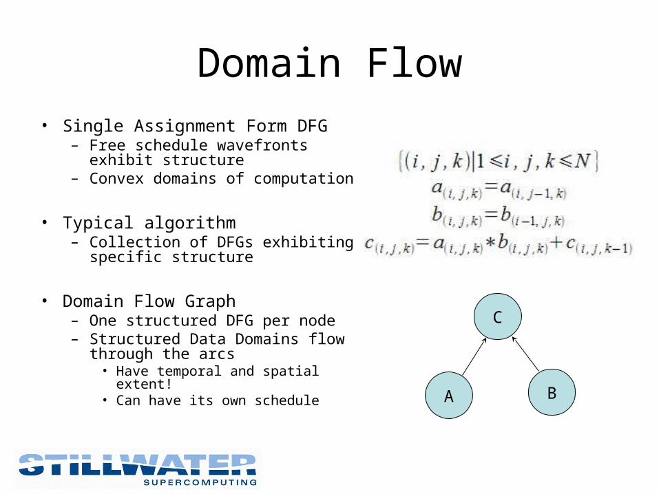
Domain Flow• Single Assignment Form DFG
– Free schedule wavefronts exhibit structure
– Convex domains of computation
• Typical algorithm– Collection of DFGs exhibiting
specific structure
• Domain Flow Graph– One structured DFG per node– Structured Data Domains flow
through the arcs• Have temporal and spatial extent!• Can have its own schedule
C
A B

High-Performance Computing
• Computational Science– genetics, proteomics, chemistry, physics, bioinformatics
• Product Engineering – aerospace, automotive, pharmaceuticals, digital content
creation, energy, process industry
• Business Analytics – BI, Risk Analysis, Trading Systems, Insurance
HPC has insatiable demand for high-fidelity computes
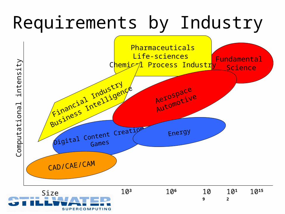
Fundamental Science
Size
Com
puta
tiona
l int
ensi
ty
103 109 1012
PharmaceuticalsLife-sciences
Chemical Process Industry
Digital Content Creation
Games
Financial Industry
Business Intelligence
1015106
Requirements by Industry
Aerospace
Automotive
CAD/CAE/CAM
Energy

Computational Science Needs
• Geometry and meshing– Roughly 1 Tops per million cells– Limited task level parallelism at 8-16 threads– High integer/control content, arbitrary precision floating
point– Multi-core CPU performance is paramount
• Solver– Roughly 1 GFlops per million cells per time step– Demand grows exponentially
• Need 10x compute power for doubling of resolution– Global schedules needed to hide memory latency– Fine-grained MIMD parallelism, high-fidelity floating
point and massive memory bandwidth are paramount• Visualization
– Roughly 50 MFlops per million pixels per frame– Demand grows polynomial– Low-fidelity floating point and massive memory
bandwidth are paramount

What are the pain points?• Computer models are limited by solver
– 80% of run-time is spent in solver– Efficiency on CPU and GPU is poor
• Typically less than 5% of peak performance
• Cost of computer clusters is too high– Millions of scientists and engineers are left out– No ecosystem of solutions can develop
• HPC does not connect with volume markets– No standard hardware and software systems– Fundamental algorithms are different– No economies of scale

Economic Forces on CPU Evolution• General Purpose Computing is inefficient
for HPC– Typically only 5% of peak performance
• CPUs favor integer and control operations– CSE needs Floating Point operations– FPU = Floating Point Unit– Typical CPU allocates less than 5% to FPU
• Die photo: Tiny blocks in top left and top right– Chip resources allocated for OS, database
and web server workloads, not CSE
• CPUs can only exploit limited parallelism through multi-core
– CSE needs 1000s of cores
• Volume design points limits I/O bandwidth– I/O Bandwidth is essential for HPC
Multi-core CPUs cannot deliver performance improvements needed for CSE innovation
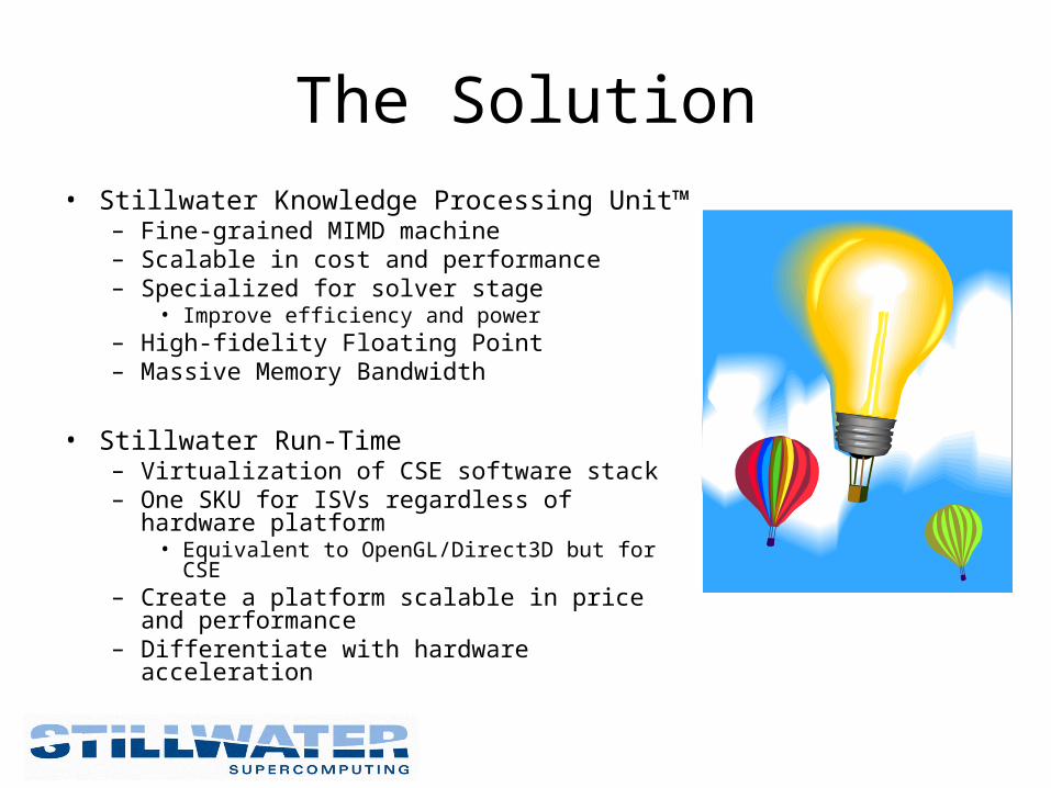
The Solution• Stillwater Knowledge Processing Unit™
– Fine-grained MIMD machine– Scalable in cost and performance– Specialized for solver stage
• Improve efficiency and power– High-fidelity Floating Point– Massive Memory Bandwidth
• Stillwater Run-Time– Virtualization of CSE software stack– One SKU for ISVs regardless of hardware
platform• Equivalent to OpenGL/Direct3D but for CSE
– Create a platform scalable in price and performance
– Differentiate with hardware acceleration

Stillwater Technology Roadmap
• Disclaimer: competitor performance is estimated based on current product or product announcements and historical performance improvements
Stillwater Performance scales better as compared to Competition
1600
2560
4096
0
500
1000
1500
2000
2500
3000
3500
4000
4500
2007 2008 2009 2010 2011
Year of Production
Peak
Perf
orm
ance
(G
flops/
sec)
Stillwater KPU Intel multi-core
IBM Cell NVIDIA Tesla
Stillwater T1
Stillwater T2
Stillwater T4

Stillwater Supercomputing Value Proposition
• Dramatically Reduce Cost of HPC: 10/10/10– 10T Flops/sec workstation for $10k by 2010– Expand the Computational Science and
Engineering (CSE) community
• Focus on CSE Opportunity– Computational demands grow exponentially– Efficiency is paramount– Large, important, and captive audience
• Enable Interactivity: iCSE– Interactivity improves productivity– Better for creativity and innovation– Exclusive solution for interactive science,
engineering, and BI applications

Acceleration is the only economic way to address submarkets
• Incur costs only for target market– Massive memory bandwidth– High-fidelity floating point– Fine-grained MIMD parallelism
• Leverage economies of scale for common components– PC hardware and software ecosystem
• Add value at reasonable cost– PC cost targets not Supercomputing
prices

• Product Introduction in 2H 2009– Stillwater T1 KPU
– 65nm/100 mm2
– 1.6T SP Flops/sec, 0.8 DP Flops/sec
• Board Level product– $500 PCI-Express Gen 2 AIC
– 1, 2, or 4 KPUs
– 2, 4, or 8 GBytes memory, GDDR 5
– 1, 2, or 4 TFlops/sec per AIC
• Follow on product in 2H 2010– Stillwater T2 KPU
– 55nm/100 mm2
– 2.56 TFlops/sec
• Board Level Product in 2010– First ever 10TFlops/sec AIC with 4 KPUs
Stillwater Supercomputing Products

End-user Solutions