Does Price Matter? Price and Non-Price Competition in the ...fmDoes Price Matter? Price and Non-Price Competition in the Airline Industry Philip G. Gayle∗ Kansas State University

Does Price Matter? Price and Non-PriceCompetition in the Airline Industry

Philip G. Gayle∗

Kansas State University

May 3, 2004

Abstract

This paper studies passengers’ choice behavior in air travel. Products are de-fined as a unique combination of airline and flight itinerary while markets aredefined as a directional round-trip air travel between an origin and a destina-tion city. A structural econometric model is used to investigate the relativeimportance of price (airfare) and non-price product characteristics in explainingpassengers’ choice of these differentiated products. The results suggest that, onaverage, prices may not be as important as we think in explaining passengers’choice behavior among alternative products. Non-price characteristics whichmay include convenience of flight schedules, frequent flyer programs, the qualityof in-flight service, among other things, seem to be much more important in ex-plaining passengers’ choice behavior. As such, the results have implications forthe focus of antitrust policies in the airline industry when assessing the impactof mergers, alliances, or other business decisions of airlines.

JEL Classification: L13, L93, C1, C2Keywords: Discrete Choice, Mixed Logit, Airlines, Hub and Spoke Network,Frequent Flyer Programs

∗Department of Economics, 327 Waters Hall, Kansas State University, Manhattan, KS, 66506,(785) 532-4581, Fax:(785) 532-6919, email: [email protected].

1 Introduction.

Probably two of the most important developments in the U.S. airline industry follow-

ing deregulation in 1978, were the airlines’ move to hub-and-spoke networks and their

increased sophistication in pricing and marketing their products [Borenstien(2004)].

The hub-and-spoke network has the effect of increasing the dominance of a few air-

lines in markets where these airlines have hubs in big cities [see Borenstein (1992)]. A

hub network allows airlines to offer change-of-plane service between airports for which

the hub is a convenient intermediate stop. As such, strategically establishing hubs

in various cities constitutes one aspect of non-price competition that exists between

airlines. Sophistication in marketing practices such as frequent flyer programs and

travel agent commission override programs1 are other examples of non-price aspects

of competition that serves to increase an airline’s dominance.

Despite the numerous non-price aspects of competition among airlines, the focus

of policy makers is often on the potential price effects that various business decisions

of airlines may have. Examples of airline business decisions that often concern policy

makers include mergers and code share alliances among airlines. One of the main

objectives of this paper is to emphasize the importance of controlling for the non-price

aspects of competition among airlines’ when assessing the price effects of business

strategies of these airlines. In fact, the relative importance that policy makers place

on the price effects of proposed or actual business strategies of airlines may even be

in question.

It is well known that in industries where products are not homogenous, compe-

tition among firms is not restricted to price.2 In fact, the non-price characteristics

of products may be just as important as price, if not more so, in explaining con-

sumers’ choice of particular products. As suggested above, the airline industry is

1Frequent flyer programs normally involve passengers’ ability to use accumulated miles traveledon an airline to qualify for discounts on tickets while travel agent commission override programsinvolve arrangements where agents are rewarded for directing a high proportion of their bookings tothe airline.

2See the chapter on product differentiation in Tirole (1988). In the tenth printing of the text,the relevant discussion is found in chapter 7.

1

one example of a differentiated product industry where firms compete on various

non-price characteristics of the products offered. For example, in addition to the fre-

quent flyer programs and the travel agent commission override programs mentioned

above, airlines may offer multiple itineraries3 within a given market, and various pro-

motional activities4 designed to steal customers from competitors. A frequent flyer

program is an example of loyalty-inducing marketing device that is intended to reduce

consumer’s sensitivity to price. Empirical studies by Nako (1992), Proussaloglou and

Koppelman (1995), and Suzuki et al. (2003) have shown that frequent flyer programs

significantly affect travelers’ choice of airlines. In the face of the non-price product

characteristics that may influence consumers’ choice of a product, which then drives

the multidimensional nature of competition in the airline industry, one may wonder

how important price is as a strategic variable for airlines.

Knowing potential passengers’ relative valuation of various product characteris-

tics must be at the heart of formulating effective business strategies. Acquiring this

information is confounded by the fact that passengers are heterogeneous, that is,

each passenger is likely to have a different valuation for each product characteristic.

As such, explicitly modeling potential passengers’ decision making process is crucial

in any attempt to estimate the relative importance of price in the multidimensional

nature of competition between airlines. Thanks to recent advances in economet-

ric estimation of demand for differentiated products, [Berry, Levinsohn, and Pakes

(1995) popularly referred to as BLP, Berry(1994), Nevo(2000)] consumer heterogene-

ity can explicitly be incorporated in a structural econometric model of consumer

decision making process. To my knowledge, except for Berry, Carnall, and Spiller

(1997) (henceforth BCS), there has not been any other attempt to explicitly model

passengers’ heterogeneity within a discrete choice econometric model of demand for

air travel. One crucial difference between the model in this paper and the BCS

model is that here, consumers’ heterogeneity (variation in taste) is allowed to vary

3Multiple times of departures and arrivals combined with variations in intermediate stops.4Advanced purchase of tickets, stopover deals etc.

2

with demographic information (such as income and age) drawn from each market,5

while in BCS, heterogeneity solely depends on an assumed parametric distribution of

taste.

The rest of the paper is organized as follows. The empirical model is presented

in section 2. There, I discuss how passengers’ heterogeneity is modeled, which has

implications for estimating the model. Section 3 discusses the estimation strategy

along with my identifying assumptions. I discuss characteristics of the data in section

4 and results are presented and discussed in section 5. Even though the analysis

in this paper focuses on a sample of U.S. domestic air travel markets, the research

methodology can easily be extended to international air travel. Concluding remarks

are made in section 6.

2 The Model.

In the model, a market is defined as a directional round-trip air travel between an

origin and a destination city. The assumption that markets are directional implies

that a round-trip air travel from Atlanta to Dallas is a distinct market than round-

trip air travel from Dallas to Atlanta. This allows characteristics of origin city to

affect demand [see BCS]. In what follows, markets are indexed by t .

A flight itinerary is defined as a specific sequence of airport stops in getting from

the origin to destination city. Products are defined as a unique combination of airline

and flight itinerary.6 For example, three separate products are (1) a non-stop round

trip from Atlanta to Dallas on Delta Airlines, (2) a round trip from Atlanta to Dallas

with one stop in Albuquerque on Delta Airlines, and (3) a non-stop round trip from

Atlanta to Dallas on American Airlines. Note that all three products are in the

same market. The airline specific component of the product definition is intended

5See Nevo(2000) for more on this approach.6Even though it is possible to further distinguish products by using a unique combination of price,

airline and flight itinerary as in BCS, I chose to use only airline and flight itinerary. The reason isthat observed product market shares, which I define subsequently, will be extremely small if productsare defined too narrowly. The empirical model becomes difficult to fit when product market sharesare extremely small.

3

to capture the fact that airlines differ in the service they offer. Airline services may

differ along several dimensions. For example, frequent flyer programs and the quality

of in-flight service often differ across airlines.

Let consumer i choose among J different products offered in market t by com-

peting airlines. The indirect utility that consumer i gets from consuming a product

in market t is given by

Uijt = dj + xjtβi − αipjt +4ξjt + εijt (1)

where dj are product fixed effects capturing characteristics of the products that are

the same across markets, xjt is a vector of observed product characteristics, βi is a

vector of consumer taste parameters (assumed random) for different product charac-

teristics, pjt is the price of product j , αi represents the marginal utility of price, 4ξjt

are differences in unobserved (by the econometrician) product characteristics since

dj is included in equation(1), and εijt represents the random component of utility

that is assumed independent and identically distributed across consumers, products

and markets. The product characteristics captured by dj may include, but not re-

stricted to, the quality of in-flight service, and frequent flyer programs offered by each

airline. 4ξjt is defined as differences in unobserved product characteristics because

4ξjt = ξjt− ξj , where ξjt represents unobserved product characteristics of product j

in market t, and ξj represents the portion of the unobserved product characteristics

of product j that is the same across all markets. By including dj in the model, I

have basically controlled for ξj [see Nevo(2000), Villas-Boas(2003)].7

Note that βi and αi are individual specific, implying that consumers have different

taste for each product characteristic. For example, consumers may differ on their

preference for a particular flight itinerary which may involve multiple stops. The

difference in preference may depend on the consumers’ age, opportunity cost of time

(income), and other unobservable (by the econometrician) taste components. Follow-

ing Nevo(2000), I assume that individual characteristics consist of two components:

7dj is captured by a set of airline dummies. The implications of including these dummies in themodel will become clearer in the estimation section where I discuss instrumental variables.

4

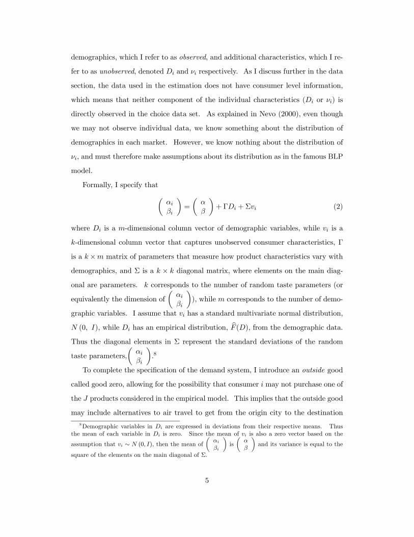
demographics, which I refer to as observed, and additional characteristics, which I re-

fer to as unobserved, denoted Di and νi respectively. As I discuss further in the data

section, the data used in the estimation does not have consumer level information,

which means that neither component of the individual characteristics (Di or νi) is

directly observed in the choice data set. As explained in Nevo (2000), even though

we may not observe individual data, we know something about the distribution of

demographics in each market. However, we know nothing about the distribution of

νi, and must therefore make assumptions about its distribution as in the famous BLP

model.

Formally, I specify thatµαiβi

¶=

µαβ

¶+ ΓDi +Σvi (2)

where Di is a m-dimensional column vector of demographic variables, while vi is a

k-dimensional column vector that captures unobserved consumer characteristics, Γ

is a k×m matrix of parameters that measure how product characteristics vary with

demographics, and Σ is a k × k diagonal matrix, where elements on the main diag-

onal are parameters. k corresponds to the number of random taste parameters (or

equivalently the dimension ofµ

αiβi

¶), while m corresponds to the number of demo-

graphic variables. I assume that vi has a standard multivariate normal distribution,

N (0, I), while Di has an empirical distribution, bF (D), from the demographic data.

Thus the diagonal elements in Σ represent the standard deviations of the random

taste parameters,µ

αiβi

¶.8

To complete the specification of the demand system, I introduce an outside good

called good zero, allowing for the possibility that consumer i may not purchase one of

the J products considered in the empirical model. This implies that the outside good

may include alternatives to air travel to get from the origin city to the destination

8Demographic variables in Di are expressed in deviations from their respective means. Thusthe mean of each variable in Di is zero. Since the mean of vi is also a zero vector based on the

assumption that vi ∼ N (0, I), then the mean ofµ

αiβi

¶isµ

αβ

¶and its variance is equal to the

square of the elements on the main diagonal of Σ.

5

city and back. These alternatives may include motor vehicle or train. As usual, the

mean utility level of the outside good, δ0t, is normalized to be a constant and equal

to zero, while the mean utility level of each of the J products, δjt, is given by

δjt = dj + xjtβ − αpjt +4ξjt (3)

Let θ = (Γ,Σ) be a vector of non-linear parameters. Further, let

µijt(xjt, pjt, νi, Di; θ) = [−pjt, xjt] (ΓDi +Σνi) (4)

Using equations (1) to (4) allows me to express the indirect utility from consuming

product j as

Uijt = δjt + µijt + εijt (5)

where µijt + εijt is a mean zero heteroskedastic deviation from the mean utility that

captures the effects of the random coefficients.

I assume that consumers purchase one unit of the product that gives the highest

utility. Based on the above, the vector (νi, Di, εi0t, ..., εiJt) describes the attributes

of a consumer. Formally, the set of individual attributes that lead to the choice of

product j can be written as

Ajt = {(νi, Di, εi0t, ..., εiJt) |Uijt ≥ Uilt ∀l = 0, 1, ..., J}

Thus Ajt represents the set of consumers who choose product j in market t. Re-

call that a product is defined as an itinerary-airline combination. For example, if

product j is a round-trip from Atlanta to Dallas with one stop in Albuquerque on

Delta Airlines, then Ajt defines the set of consumers choosing this itinerary-airline

combination rather than any other itinerary-airline combination in the Atlanta to

Dallas market. Formally, I can define the predicted (by the model) market share of

product j as

sjt(xjt, pjt; α, β, θ) =

ZAjt

dF (v,D, ε)

=

ZAjt

dF (v) d bF (D) dF (ε) (6)

6

where F (·) denotes the population distribution functions and F (v,D, ε) = F (v) bF (D)F (ε)is due to assumed independence of ν, D, and ε. If we assume that both D and ν are

fixed, thus implying that consumer heterogeneity enters only through the random

shock, and εijt is independent and identically distributed (i.i.d.) with an extreme

value type I density, then equation (6) becomes

sjt(xjt, pjt; α, β) =eδjt

eδ0t +JPl=1

eδlt

=eδjt

1 +JPl=1

eδlt

(7)

which is the standard multinomial logit model. If we relax the assumption that

both D and ν are fixed, while still assuming that εijt is i.i.d. type I extreme value,

equation (6) becomes

sjt(xjt, pjt; α, β, θ) =

Zeδjt+µijt

1 +JPl=1

eδlt+µijtd bF (D)dF (ν) (8)

Equation (8) corresponds to the random coefficients (or mixed logit) model that I use

in this paper. As is well known in the empirical industrial organization literature,

there is no closed form solution for equation (8) and thus it must be approximated

numerically using random draws from bF (D) and F (ν).

Recall that sjt(xjt, pjt; α, β, θ) in equation (8) is the predicted market share of

product j and therefore is not observed. Given a market size of measure M, which I

assume to be the size of the population in the origin city, observed market shares of

product j in market t is Sjt=qjM , where qj is the actual number of travel tickets sold

for a particular itinerary-airline combination called product j. The observed market

share for each product is computed analogously. The estimation strategy involves

choosing values of α, β and θ to minimize the distance between the predicted, sjt,

and observed, Sjt, market shares.

3 Estimation.

I use Nevo’s (2000) simulation based Generalized Methods of Moments (GMM) es-

timation algorithm. First, to numerically approximate equation (8), I took random

7

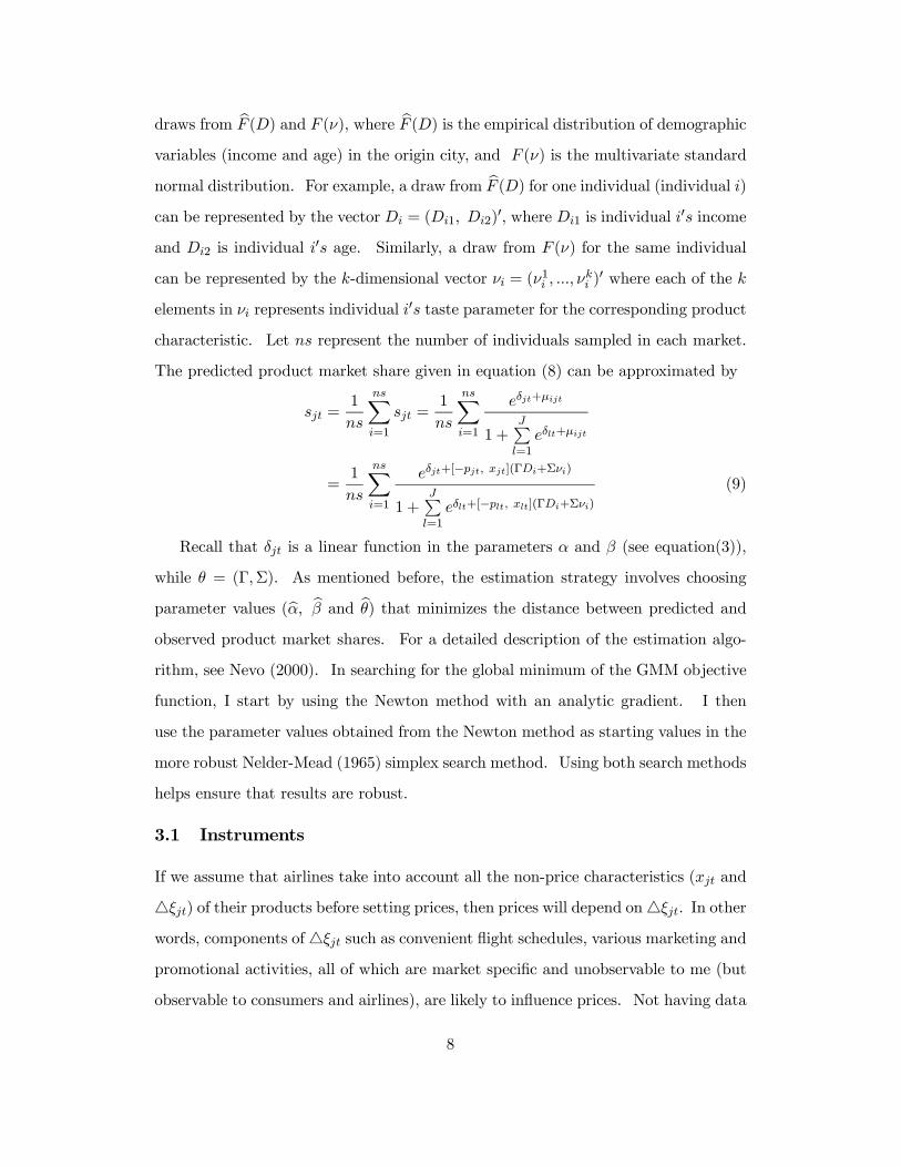
draws from bF (D) and F (ν), where bF (D) is the empirical distribution of demographicvariables (income and age) in the origin city, and F (ν) is the multivariate standard

normal distribution. For example, a draw from bF (D) for one individual (individual i)can be represented by the vector Di = (Di1, Di2)

0, where Di1 is individual i0s income

and Di2 is individual i0s age. Similarly, a draw from F (ν) for the same individual

can be represented by the k-dimensional vector νi = (ν1i , ..., νki )0 where each of the k

elements in νi represents individual i0s taste parameter for the corresponding product

characteristic. Let ns represent the number of individuals sampled in each market.

The predicted product market share given in equation (8) can be approximated by

sjt =1

ns

nsXi=1

sjt =1

ns

nsXi=1

eδjt+µijt

1 +JPl=1

eδlt+µijt

=1

ns

nsXi=1

eδjt+[−pjt, xjt](ΓDi+Σνi)

1 +JPl=1

eδlt+[−plt, xlt](ΓDi+Σνi)

(9)

Recall that δjt is a linear function in the parameters α and β (see equation(3)),

while θ = (Γ,Σ). As mentioned before, the estimation strategy involves choosing

parameter values (bα, bβ and bθ) that minimizes the distance between predicted andobserved product market shares. For a detailed description of the estimation algo-

rithm, see Nevo (2000). In searching for the global minimum of the GMM objective

function, I start by using the Newton method with an analytic gradient. I then

use the parameter values obtained from the Newton method as starting values in the

more robust Nelder-Mead (1965) simplex search method. Using both search methods

helps ensure that results are robust.

3.1 Instruments

If we assume that airlines take into account all the non-price characteristics (xjt and

4ξjt) of their products before setting prices, then prices will depend on4ξjt. In other

words, components of4ξjt such as convenient flight schedules, various marketing and

promotional activities, all of which are market specific and unobservable to me (but

observable to consumers and airlines), are likely to influence prices. Not having data

8

on 4ξjt implies that it is part of the error term in the demand model. As such, the

estimated coefficient on price will be inconsistent if appropriate instruments are not

found for prices. As is well known in econometrics, valid instruments must satisfy two

requirements. First, instruments must be uncorrelated with the residual, and second,

they must be correlated with the endogenous variable that needs to be instrumented

for. In other words, valid instruments must be uncorrelated with4ξjt but correlated

with pjt. I employ two sets of instruments in estimation which I describe below.

The first set of instruments that I use is described and used in Nevo(2000) and first

introduced by Hausman et al.(1994) and Hausman (1996). This set of instruments is

an attempt to exploit the panel structure of the data. Since I observe prices charged

by each airline in a cross section of markets, the identifying assumption made is that,

controlling for the component of the service that is constant across markets (embodied

in airline dummies), the market specific valuations of the products, 4ξjt = ξjt − ξj ,

are independent across markets. This implies that 4ξjt is uncorrelated with prices

in markets other than market t. If we couple this with the idea that prices charged

by an airline across markets have a common cost component that may be specific

to the airline, then each airlines’ prices ought to be correlated across markets. The

upshot of these arguments is that prices charged by an airline in different markets

can instrument for each other. The common cost component in an airline’s prices

could result from providing a similar general quality of service across all the markets

it serves. Of course, prices are also influenced by market specific factors, such as the

level of competition in a particular market, implying that in equilibrium, an airline’s

prices should not be identical across markets. In summary, I use average prices

charged by an airline in other markets to instrument for its prices in each market.

The second set of instruments I use is described in Villas-Boas (2003). Since

input prices are marginal cost shifters, they are also valid instruments for prices of

final products. The problem in using input prices as instruments in these discrete

choice models is that input prices do not vary across brands of the product, while

final goods prices vary across brands. For example, in applying the model to the

9

yogurt market [see Villas-Boas (2003)], the price of sugar, an input for yogurt, is the

same across all brands of yogurt. Similarly, in the case of the market for air travel,

the price per gallon of fuel is the same whether the product is a round trip non-stop

flight from Atlanta to Dallas on Delta or a round trip non-stop flight from Atlanta to

Dallas on American Airlines. Notwithstanding that input prices are the same across

brands of differentiated products, Villas-Boas argued that a change in input prices

may affect different brands in different ways since brands may differ in their relative

use of inputs. Thus Villas-Boas recommend using as instruments, the interaction

between input prices and brand dummies. This allows input prices to affect the final

price of each brand differently. Following Villas-Boas (2003), I use the interaction

of fuel prices with airline dummies as instruments for final ticket prices. Similar to

Villas-Boas’s argument, the idea is that a change in fuel price may affect each airline

differently, one reason being that airlines may offer different flight itineraries in a

market that require different amounts of fuel to service each itinerary. For example,

it is reasonable to assume that an itinerary for a non-stop flight from Atlanta to

Dallas requires different amounts of fuel compared to an itinerary from Atlanta to

Dallas with one stop in Albuquerque.

4 Data.

Data on the airline industry is drawn from the Origin and Destination Survey (DB1B),

which is a 10% sample of airline tickets from reporting carriers. The U.S. Bureau

of Transportation Statistics publishes this database along with other transportation

data via its TranStats website.9 The DB1B database includes such items as passen-

gers, fares, and distances for each directional market, as well as information about

whether the market was domestic or international. Distances flown vary within a

market because itineraries may involve multiple connecting flights to get from the

origin to the destination city. A market may therefore comprise several distinct

9For detail on air travel data published by U.S. Bureau of Transportation go tohttp://transtats.bts.gov/

10

routes or segments. As such, the data I use correspond to directional markets rather

than non-stop routes or segments of a market. For this research, I focus on the U.S.

domestic market in the first quarter of 2002.

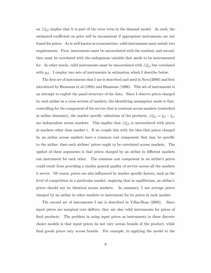
Summary statistics for the sample of air travel data are presented in table 1. The

first column lists the fifteen markets considered, while the second column gives the

number of observations (products) in each market. In the third column, I report the

percentage of products

Table 1 Summary Statistics

Market Observati-ons a

N=1462

Hub b

(%)

Mean Price ($)

Min Price ($)

Max Price ($)

Mean Distance (Miles)

Min Distance (Miles)

Max Distance (Miles)

Atlanta – Dallas 111 33.33 278.74 0 785 1112.54 731 1870 Atlanta - Newark 78 25.64 259.85 0 805 1107.03 745 1646 Atlanta - Los Angeles 181 30.94 361.82 0 2101 2491.46 1946 4158 Atlanta - Salt Lake City 160 35.00 333.92 0 1480 2271.18 1589 3763 Cincinnati - Atlanta 57 24.56 299.20 5 651 687.44 373 1105 Cincinnati - Los Angeles 62 32.26 291.75 0 1251 2349.42 1900 3383 Cincinnati - Salt Lake City 90 34.44 337.36 0 1654 2068.91 1449 3175 Dallas - Atlanta 137 31.39 303.92 0 1131 1179.53 731 1973 Dallas - Cincinnati 57 29.82 357.62 0 1183 1373.18 812 2432 Dallas - Newark 63 19.05 399.55 0 1622 1646.92 1372 2956 Houston - Cleveland 76 19.74 252.14 0 1538 1441.79 1091 2442 Houston - Newark 109 28.44 390.03 0 1280 1718.24 1400 3142 Minneapolis - Atlanta 55 3.64 240.33 0 838 1364.84 906 2096 Salt Lake City - Atlanta 151 31.13 364.26 0 1301 2293.79 1589 4684 Salt Lake City - Cincinnati 75 29.33 331.69 0 1681 2142.92 1449 3162

a Sample size of products (itinerary-airline combination) in the particular market. b The percentage of the sample of products for which the origin airport is a hub.

in the sample for which the origin airport is a hub. For example, the table shows

that of the 111 products in our sample for the Atlanta to Dallas market, Atlanta

is a hub for 33.33% of them (hub products).10 As mentioned in the introduction,

the hub-and-spoke network is one of the major developments in the airline industry

since deregulation. Hub products may offer more convenient flight schedules since

airlines normally fly to a wider range of destinations from their hub airport. As

such, the empirical model should capture this non-price component of products as

this is likely to influence passengers’ choice behavior among alternative products.

The fourth, fifth and sixth columns summarize data on airfares.11 We can see that,10Products offered by Delta airlines would be part of this 33.33% since Atlanta is a major hub

for Delta while products offered by American airlines in this market would not be included in the33.33% since Atlanta is not a hub for American.11Since each passenger may pay a different price/fare for a given itinerary-airline combination for

various reasons (advanced purchase of ticket, weekend stay over days etc.), I used the average pricepaid for a given itinerary-airline combination over the review period.

11

within a market, the minimum airfare for a ticket is zero dollars. These tickets are

likely associated with passengers using their accumulated frequent flyer miles to offset

ticket price.12 The seventh, eighth and ninth columns summarize data on distances

flown in each market.

Given that the ticket purchase data discussed above does not have passenger-

specific information, such as a passengers’ income or age, we use information on the

distribution of demographic data in the origin city to account for taste heterogeneity

in travel demand. As such, estimating equation (9) requires supplementing the ticket

purchase data with demographic data drawn from the origin city’s population in

each market.13 These demographic data are drawn from the 2001 and 2002 Current

Population Survey (CPS) published by the U.S. Bureau of Labor Statistics. Tables

2A and 2B summarize the demographic

12Unfortunately, the data does not contain information that allows me to distinguish betweentickets that were bought with frequent flyer miles. I can only observe the actual price paid for eachticket and conjecture that tickets with an unusually low price are either associated with frequent flyeror some other promotional program. In either case, I would not want to throw out these observationssince they may contain useful information about the non-price component of an airline’s products.As you will see in the results section, I use the empirical model to disentangle the price and non-priceproduct components that influence passengers’ choice behavior.13This non-parametric approach to model consumer heterogeniety is explained in more detail in

Nevo(2000).

12

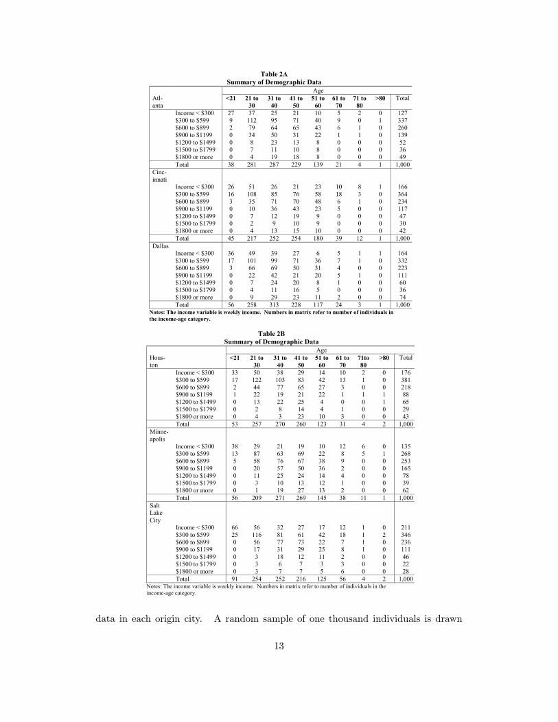
Table 2A Summary of Demographic Data

Age Atl- anta

<21 21 to 30

31 to 40

41 to 50

51 to 60

61 to 70

71 to 80

>80 Total

Income < $300 27 37 25 21 10 5 2 0 127 $300 to $599 9 112 95 71 40 9 0 1 337 $600 to $899 2 79 64 65 43 6 1 0 260 $900 to $1199 0 34 50 31 22 1 1 0 139 $1200 to $1499 0 8 23 13 8 0 0 0 52 $1500 to $1799 0 7 11 10 8 0 0 0 36 $1800 or more 0 4 19 18 8 0 0 0 49 Total 38 281 287 229 139 21 4 1 1,000 Cinc- innati

Income < $300 26 51 26 21 23 10 8 1 166 $300 to $599 16 108 85 76 58 18 3 0 364 $600 to $899 3 35 71 70 48 6 1 0 234 $900 to $1199 0 10 36 43 23 5 0 0 117 $1200 to $1499 0 7 12 19 9 0 0 0 47 $1500 to $1799 0 2 9 10 9 0 0 0 30 $1800 or more 0 4 13 15 10 0 0 0 42 Total 45 217 252 254 180 39 12 1 1,000 Dallas Income < $300 36 49 39 27 6 5 1 1 164 $300 to $599 17 101 99 71 36 7 1 0 332 $600 to $899 3 66 69 50 31 4 0 0 223 $900 to $1199 0 22 42 21 20 5 1 0 111 $1200 to $1499 0 7 24 20 8 1 0 0 60 $1500 to $1799 0 4 11 16 5 0 0 0 36 $1800 or more 0 9 29 23 11 2 0 0 74 Total 56 258 313 228 117 24 3 1 1,000

Notes: The income variable is weekly income. Numbers in matrix refer to number of individuals in the income-age category.

Table 2B Summary of Demographic Data

Age Hous- ton

<21 21 to 30

31 to 40

41 to 50

51 to 60

61 to 70

71to 80

>80 Total

Income < $300 33 50 38 29 14 10 2 0 176 $300 to $599 17 122 103 83 42 13 1 0 381 $600 to $899 2 44 77 65 27 3 0 0 218 $900 to $1199 1 22 19 21 22 1 1 1 88 $1200 to $1499 0 13 22 25 4 0 0 1 65 $1500 to $1799 0 2 8 14 4 1 0 0 29 $1800 or more 0 4 3 23 10 3 0 0 43 Total 53 257 270 260 123 31 4 2 1,000 Minne- apolis

Income < $300 38 29 21 19 10 12 6 0 135 $300 to $599 13 87 63 69 22 8 5 1 268 $600 to $899 5 58 76 67 38 9 0 0 253 $900 to $1199 0 20 57 50 36 2 0 0 165 $1200 to $1499 0 11 25 24 14 4 0 0 78 $1500 to $1799 0 3 10 13 12 1 0 0 39 $1800 or more 0 1 19 27 13 2 0 0 62 Total 56 209 271 269 145 38 11 1 1,000 Salt Lake City

Income < $300 66 56 32 27 17 12 1 0 211 $300 to $599 25 116 81 61 42 18 1 2 346 $600 to $899 0 56 77 73 22 7 1 0 236 $900 to $1199 0 17 31 29 25 8 1 0 111 $1200 to $1499 0 3 18 12 11 2 0 0 46 $1500 to $1799 0 3 6 7 3 3 0 0 22 $1800 or more 0 3 7 7 5 6 0 0 28 Total 91 254 252 216 125 56 4 2 1,000

Notes: The income variable is weekly income. Numbers in matrix refer to number of individuals in the income-age category.

data in each origin city. A random sample of one thousand individuals is drawn

13

from each origin city’s population. From the samples drawn, we can see that there

is some diversity within each city. For example, while the majority of the sample

between ages 21 and 40 have weekly income below $1,200, quite a few people in this

age group earn above $1,200 per week. Further, most individuals above the age of

60 have income below $1,200 per week. When faced with the same set of options,

it is likely that these distinct groups of potential passengers may make different

product choices. One reason is that they may have different tastes over prices and

flight schedule convenience. The empirical model is designed to account for such

passenger heterogeneity.

5 Results.

Recall that non-price product characteristics are captured by xjt and dj [see equation(1)],

where the researcher can observe variables in xjt but not dj . However, passengers and

airlines both observe xjt and dj . The variables in xjt are “Hub”, “Hub×Distance”,and “Distance×Market t”, all of which are explained below. dj are product fixed

effects capturing product characteristics that are the same across markets. As I

mentioned before, these unobserved product characteristics may include, but not re-

stricted to, the quality of in-flight service, and frequent flyer programs offered by

each airline. Including airline dummies in the estimation is sufficient to control for

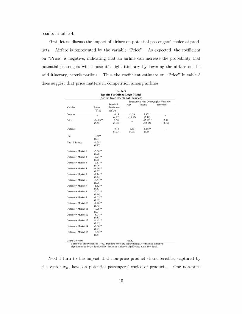
dj . First, I estimate the mixed logit model (equation (9)) using pjt and xjt as the

independent variables. These results are displayed in table 3.14 I then re-estimate

the model using pjt, xjt and a full set of airline dummies as independent variables.

The results when airline dummies are included in the estimation are displayed in

table 4. A comparison of the results across both tables has implications for the

importance of price competition after controlling for unobservable non-price product

characteristics. Results in table 3 are discussed first, then I compare and discuss the

14The coefficients in table 3 correspond to the parameters in equation(9) as follows. α is the coeffi-cient on “Price”. The parameter vector β corresponds to the coefficients on “Hub”, “Hub×Distance”,“Distance×Market t” for t = 1, 2, ..., 15. The parameters in the Σ matrix correspond to the coeffi-cients in the column labeled “Standard Deviations”. The parameters in the Γ matrix correspond tothe coefficients in the last three columns labeled, “Age”, “Income”, and “(Income)2”.

14

results in table 4.

First, let us discuss the impact of airfare on potential passengers’ choice of prod-

ucts. Airfare is represented by the variable “Price”. As expected, the coefficient

on “Price” is negative, indicating that an airline can increase the probability that

potential passengers will choose it’s flight itinerary by lowering the airfare on the

said itinerary, ceteris paribus. Thus the coefficient estimate on “Price” in table 3

does suggest that price matters in competition among airlines.

Table 3 Results For Mixed Logit Model

(Airline fixed effects not Included) Interactions with Demographic Variables:

Variable

Mean

)'( sβ

Standard Deviations

)'( sσ

Age Income (Income)2

Constant _ -0.13 (4.87)

-3.39 (10.52)

7.95** (2.18)

_

Price -14.83** (5.62)

2.50 (3.48)

_ -45.68** (22.52)

13.39 (14.19)

Distance _ -0.18 (1.32)

3.51 (4.00)

-8.18** (1.38)

_

Hub 1.30** (0.37)

Hub×Distance -0.28* (0.17)

Distance×Market 1

-3.66** (1.28)

Distance×Market 2 -3.24** (1.35)














GMM Objective

369.82

Number of observations is 1,462. Standard errors are in parentheses. ** indicates statistical significance at the 5% level, while * indicates statistical significance at the 10% level.

Next I turn to the impact that non-price product characteristics, captured by

the vector xjt, have on potential passengers’ choice of products. One non-price

15

characteristic that I do observe is whether or not the origin airport is a hub for the

airline offering the product. Two possible reasons why passengers are more likely

to choose itineraries offered by hub airlines are: (1) flight schedules offered by hub

airlines may be more convenient (less intermediate stops), (2) it is more likely that

passengers have frequent flyer membership with a hub airline.15 The variable “Hub”

is a dummy variable taking the value one if the product is offered by an airline that

has a hub at the origin airport and zero otherwise. The coefficient on “Hub” is

positive, indicating that potential passengers are more likely to choose itineraries

where the origin airport is a hub for the airline offering the itinerary. In other words,

airlines have a strategic advantage at their hub airports compared to their non-hub

competitors.

Another non-price characteristic that influences passengers’ choice of products is

the convenience of flight schedule embodied in the itinerary. I measure the conve-

nience of a schedule by the actual distance flown in getting from the origin to the

destination airport.16 The actual distance flown to get to a destination from a specific

origin may vary since itineraries do not always involve direct flights from the origin

to the destination. For example, in the market where Kansas City is the origin and

San Diego is the destination, an itinerary which has one intermediate stop in Chicago

involve flying a longer distance compared to an itinerary with one intermediate stop

in Phoenix. Note however that even though both itineraries involve one intermediate

stop, they may differ in terms of distance flown. I associate shorter distances with

more convenient schedules. A direct flight from Kansas City to San Diego would

involve the shortest possible distance in this market and thus interpreted as the most

convenient schedule in the said market. The variables in table 3 that capture this

15See Proussaloglou and Koppelman (1995), Schumann (1986).16Subject to the availability of detailed data, we may measure the convenience of flight schedules

in several ways. For example, information on departures and arrival times allows the researcher tocompute total layover time associated with each itinerary. A second alternative to measure scheduleconvenience is to use a count of the number of intermediate stops associated with each itinerary.Third, the researcher could use the actual distance flown on each itinerary in a given market. I optto use the actual distance flown as a measure of schedule convenience since it is arguably a superiormeasure compared to number of intermediate stops (see discussion in text) and I did not have dataon arrival and departure times for each itinerary which rules out using layover times.

16

measure of schedule convenience are the interactions between “Distance” and “Mar-

ket”. The variables “Market” are dummies taking the value one if the product is

in the relevant market and zero otherwise. The coefficients on the interactions be-

tween “Distance” and “Market” dummies are negative, indicating that within a given

market (origin-destination combination), passengers prefer to choose flight itineraries

that cover shorter distances, ceteris paribus.

The coefficient on the interaction between “Hub” and “Distance” also uncovers

an interesting result. This coefficient is negative, indicating that passengers are more

likely to choose hub products that have the shortest possible distance. Even more

important, it reveals that passengers are more sensitive to distance flown (schedule

convenience) for hub products compared to non-hub products. In other words, pas-

sengers may expect hub itineraries to involve shorter distances (be more convenient)

and thus hub itineraries involving longer distances (less convenient) are more heavily

penalized compared to non-hub itineraries with equivalently long distances.

It is well known that consumers are heterogenous with respect to their taste for

various characteristics of differentiated products. As such, diversity in tastes often

leads to diversity in products offered and purchased. Accounting for heterogeneity in

taste is at the heart of the mixed logit model [see BLP, Nevo(2000)]. Since consumers’

tastes are unobserved by the researcher, heterogeneity in tastes are often captured

by parametric assumptions along with non-parametric treatment of demographic in-

formation.17 Demographic information such as age and income are likely to be

correlated with taste and thus may explain consumers’ choice of differentiated prod-

ucts. Since air travel is a differentiated product industry, demographic information

may be able to explain the choices that potential passengers with a specific demo-

graphic profile may make. I now turn to the task of discussing how demographics

of potential passengers in the relevant market might influence their air travel choice

behavior.17Detail on how passengers’ heterogeniety is modeled in this paper is given in section 2. Specifically,

see equations (2), (4 ) and (8 ).

17

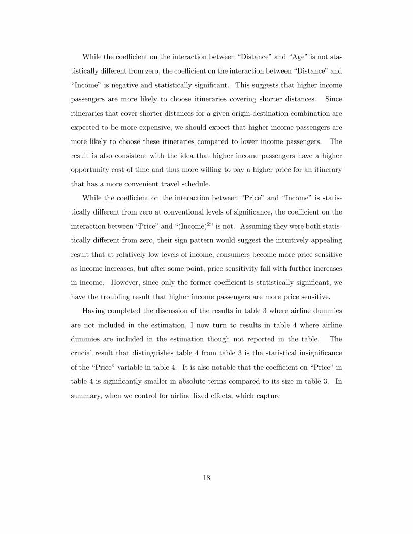
While the coefficient on the interaction between “Distance” and “Age” is not sta-

tistically different from zero, the coefficient on the interaction between “Distance” and

“Income” is negative and statistically significant. This suggests that higher income

passengers are more likely to choose itineraries covering shorter distances. Since

itineraries that cover shorter distances for a given origin-destination combination are

expected to be more expensive, we should expect that higher income passengers are

more likely to choose these itineraries compared to lower income passengers. The

result is also consistent with the idea that higher income passengers have a higher

opportunity cost of time and thus more willing to pay a higher price for an itinerary

that has a more convenient travel schedule.

While the coefficient on the interaction between “Price” and “Income” is statis-

tically different from zero at conventional levels of significance, the coefficient on the

interaction between “Price” and “(Income)2” is not. Assuming they were both statis-

tically different from zero, their sign pattern would suggest the intuitively appealing

result that at relatively low levels of income, consumers become more price sensitive

as income increases, but after some point, price sensitivity fall with further increases

in income. However, since only the former coefficient is statistically significant, we

have the troubling result that higher income passengers are more price sensitive.

Having completed the discussion of the results in table 3 where airline dummies

are not included in the estimation, I now turn to results in table 4 where airline

dummies are included in the estimation though not reported in the table. The

crucial result that distinguishes table 4 from table 3 is the statistical insignificance

of the “Price” variable in table 4. It is also notable that the coefficient on “Price” in

table 4 is significantly smaller in absolute terms compared to its size in table 3. In

summary, when we control for airline fixed effects, which capture

18

Table 4 Results For Mixed Logit Model (Airline fixed effects Included)

Interactions with Demographic Variables: Variable

Mean

)'( sβ

Standard Deviations

)'( sσ

Age Income (Income)2

Constant _ 0.08 (9.65)

1.16 (33.91)

4.55 (2.78)

_

Price -5.59 (25.31)

0.55 (6.64)

_ -15.37 (66.56)

-1.72 (23.91)

Distance _ 0.10 (2.05)

3.35 (9.08)

-1.65 (3.89)

_

Hub 0.86 (0.63)

Hub×Distance -0.48* (0.26)

Distance×Market 1

-1.00 (0.67)

Distance×Market 2 -0.68 (0.67)

Distance×Market 3 -1.13* (0.64)













GMM Objective

82.55

Number of observations is 1,462. Standard errors are in parentheses. ** indicates statistical significance at the 5% level, while * indicates statistical significance at the 10% level.

unobserved18 differences in full service packages across airlines, price becomes less

important in explaining passengers’ choice between flight itineraries offered by various

airlines. A chi-square test of the restriction between the models in tables 3 and

4 rejects the null hypothesis that the restriction is insignificant.19 This further

18Again, I want to emphasize that full service packages offered by airlines are most likely observedby or known to potential passengers before they choose among alternative products. However, theresearcher does not observe all the dimensions of the service offered by these airlines.19This chi-square test is atributed to Newey and West(1987). It posits that (n · qr − n · qur) d−→

χ2[J], where n is the sample size, qr is the value of the GMM objective for the restricted model,qur is the value of the GMM objective for the unrestricted model, and J is the number of pa-rameter restrictions. In this case J = 11 since there are eleven dummies, one for each airline.(n · qr − n · qur) = 419988.74 while the critical χ2 value at the 95% level of significance with elevendegrees of freedom is 19.68.

19

suggests that non-price characteristics of travel service offered by airlines are crucial

in explaining passengers’ choice of these services. It is also worth mentioning that

the observable non-price product characteristics still have some explanatory power,

even though somewhat reduced, after unobservable differences in full service packages

across airlines are controlled for.

6 Conclusion.

This paper illustrates the relative importance of price and non-price product char-

acteristics in influencing potential passengers choice of products offered by airlines.

The results suggest that, on average, prices may not be as important as we think in

explaining passengers choice behavior among alternative products. Non-price prod-

uct characteristics such as whether or not the product is offered by a hub airline,

convenience of flight schedules, and differences in other services offered by airlines

which may include quality of in-flight service and frequent flyer programs, are likely

to do a better job of explaining passengers choice behavior.

The findings have implications for applying antitrust policy to the airline industry

since these policies are often concerned with the potential price effect of proposed

business decisions of airlines such as mergers and alliances. If the objective of policies

is to improve or prevent the decline in welfare, then non-price product characteristics

of products offered by airlines seem to have a larger impact on welfare compared to

price. In other words, policy makers may want to focus on the impact that mergers,

alliances, or any other business decisions have on the non-price product characteristics

offered by airlines. For example, we may want to know how do mergers and alliances

affect the convenience of flight schedules offered,20 or the impact on the value of

20Richard (2003) did an excellent job estimating the impact of mergers on flight frequency. Heshows that airline mergers, while causing prices to increase, also leads to increases in flight frequencywhich may result in net increases in consumer surplus. Previous research almost exclusively focuson the price and resulting welfare effects of airline mergers [ see Borenstein (1990), Kim and Singal(1993), Werden et al. (1991), Brueckner et al. (1992), Morrison (1996)]. Papers by Brueckner(2001), Brueckner and Whalen (2000), and Bamberger et al. (2000) provide excellent analyses of theeffects of airline alliances on airfare.

20

frequent flyer programs to passengers.21 One direction that future research may

take is to assess the impact that mergers and alliances have on various non-price

product characteristics of products offered by airlines.

21Airline alliances often allow passengers to accumulate frequent flyer miles accross alliance part-ners. This is likely to improve the value of frequent flyer programs to passengers.

21

References[1] Bamberger, G., D. Carlton, L. Neuman (2000). “An Empirical Investigation of

the Competitive Effects of Domestic Airline Alliances,” NBER Working Paper#W8197.

[2] Berry, S., (1994). “Estimating Discrete-Choice Models of Product Differentia-tion,” RAND Journal of Economics, Vol. 25, 242-262.

[3] Berry, S., M. Carnall, and P. Spiller, (1997). “Airline Hubs: Cost, Markups andthe Implications of Customer Heterogeneity,” NBER working paper, No. 5561.

[4] Berry, S., Levinsohn, J., and A. Pakes. (1995). “Automobile Prices in MarketEquilibrium,” Econometrica, Vol. 63, 841-990.

[5] Borenstien, S. (2004). “Rapid Price Communication and Coordination: TheAirline Tariff Publishing Case,” in J. Kwoka and L. White, The Antitrust Rev-olution, fourth edition, Oxford University Press, 233-251.

[6] Borenstien, S. (1992). “The Evolution of U.S. Airline Competition,” Journal ofEconomic Perspectives, Vol. 6, 45-73.

[7] Borenstien, S. (1990). “Airline Mergers, Airport Dominance, and Market Power,”American Economic Review, Papers and Proceedings Vol. 80, 400-404.

[8] Brueckner, J. (2001). “The Economics of International Codesharing: An Analy-sis of Airline Alliances,” International Journal of Industrial Organization, Vol.19, 1475-1498.

[9] Brueckner, J. and W.T. Whalen (2000). “The Price Effects of InternationalAirline Alliances,” Journal of Law and Economics, Vol. XLIII, 503-545.

[10] Brueckner, J., N. Dyer, and P. Spiller (1992). “Fare determination in Airlinehub-and-spoke networks,” Rand Journal of Economics, Vol. 23, 309-333.

[11] Hausman, J., (1996). “Valuation of New Goods Under Perfect and ImperfectCompetition,” in T. Bresnahan and R. Gordon, eds., The Economics of NewGoods, Studies in Income and Wealth, Vol. 58, Chicago: National Bureau ofEconomic Research.

[12] Hausman, J., G. Leonard, and J.D. Zona, (1994). “Competitive Analysis withDifferentiated Products,” Annales d’Economie et de Statistique, 34, 159-180.

[13] Kim, E.H., and V. Singal, (1993). “Mergers and Market Power: Evidence fromthe Airline Industry,” American Economic Review, Vol. 83, 549-569.

[14] Morrison, S., (1996). “Airline Mergers: A Longer View,” Journal of TransportEconomics and Policy, Vol. 30, 237-250.

[15] Nako, S.M. (1992). “Frequent Flyer Programs and Business Travelers: An Em-pirical Investigation,” Logistics and Transportation Review 28(4), 395-414.

[16] Nelder, J. A., and R. Mead, (1965). “A Simplex Method for Function Minimiza-tion,” Computer Journal, Vol 7, 308-313.

[17] Nevo, A., (2000). “A Practitioner’s Guide to Estimation of Random CoefficientsLogit Models of Demand,” Journal of Economics and Management Strategy,9(4), 513-548.

22

[18] Newey, W., and K. West (1987). “Hypothesis Testing with Efficient Method ofMoments Estimation,” International Economic Review, Vol 28, 777-787.

[19] Proussaloglou, K., Koppelman, F. (1995). “Air Carrier Demand: An Analysis ofmarket Share Determinants,” Transportation, 22, 371-388.

[20] Richard, O., (2003). “Flight Frequency and Mergers in Airline Markets,” Inter-national Journal of Industrial Organization, Vol. 21, 907-922.

[21] Schumann, H., (1986). “Oligopolistic Nonlinear Pricing - A Study of TradingStamps and Airline Frequent Flyer Programs,” Unpublished Ph.D. Dissertation,Northwestern University.

[22] Suzuki, Y., Crum, M.R., Audino, M.J. (2003). “Airport Choice, Leakage, andExperience in Single-Airport Regions,” Journal of Transportation Engineering,forthcoming.

[23] Tirole, J., (1988). “The Theory of Industrial Organization,” The MIT Press.

[24] Villas-Boas, S., (2002). “Vertical Contracts Between Manufacturers and Retail-ers: An Empirical Analysis,” University of California, Berkeley, Manuscript.

[25] Werden, G., A. Joskow, and R. Johnson (1991). “The Effects of Mergers onPrice and Output: Two Case Studies from the Airline Industry,” Managerialand Decision Economics, Vol. 12, 341-352.

23

Documents

Does Price Matter? Price and Non-Price Competition in the ...fmDoes Price Matter? Price and Non-Price Competition in the Airline Industry Philip G. Gayle∗ Kansas State University