FEDERAL RESERVE BANK OF SAN FRANCISCO

WORKING PAPER SERIES

Working Paper 2008-16 http://www.frbsf.org/publications/economics/papers/2008/wp08-163bk.pdf

The views in this paper are solely the responsibility of the authors and should not be interpreted as reflecting the views of the Federal Reserve Bank of San Francisco or the Board of Governors of the Federal Reserve System.

The Adjustment of Global External Balances: Does

Partial Exchange Rate Pass-Through to Trade Prices Matter?

Christopher Gust

Federal Reserve Board

Sylvain Leduc Federal Reserve Bank of San Francisco

Nathan Sheets

Federal Reserve Board

June 2008

The Adjustment of Global External Balances: DoesPartial Exchange Rate Pass-Through to Trade Prices

Matter?∗

Christopher Gust†

Federal Reserve BoardSylvain Leduc

Federal Reserve Bank of San Francisco

Nathan SheetsFederal Reserve Board

June 2008

Abstract

This paper assesses whether partial exchange rate pass-through to trade priceshas important implications for the prospective adjustment of global external imbal-ances. To address this question, we develop and estimate an open-economy DGEmodel in which pass-through is incomplete due to the presence of local currencypricing, distribution services, and a variable demand elasticity that leads to fluctu-ations in optimal markups. We find that the overall magnitude of trade adjustmentis similar in a low and high pass-through world with more adjustment in a low pass-world occurring through a larger response of the exchange rate and terms of traderather than real trade flows.

Keywords: Exchange rate pass-through, Trade prices, Trade balance

JEL classification: F3, F41

∗The authors thank Chris Erceg, Joseph Gagnon, Luca Guerrieri, Dale Henderson, Karen Johnson, StevenKamin, Jaime Marquez, and Trevor Reeve for useful comments and suggestions. The views expressed in thispaper are solely the responsibility of the authors and should not be interpreted as reflecting the views of theBoard of Governors of the Federal Reserve System or of any other person associated with the Federal ReserveSystem.†Corresponding Author: Christopher Gust, Address: Federal Reserve Board, Mail Stop 42, Washington

DC, 20551, Telephone: 202-452-2383, Fax: 202-872-4926. Email addresses: christopher.gust@frb.gov andnathan.sheets@frb.gov.

1

1 Introduction

The U.S. current account deficit widened significantly over the past 15 years, reaching more

than 6 percent of GDP in 2006. This situation has raised concerns among policymakers about

how the deficit may unwind, with some observers arguing that the turnaround in the current

account deficit could be dramatic, triggering a large dollar depreciation and significant sectoral

adjustment along the way.1 Although the relative flexibility of U.S. labor markets and compet-

itiveness of the U.S. economy in general may help during the adjustment process, policymakers

worry that the presence of other frictions could hinder the adjustment of the trade balance.

One such often-mentioned friction is the well-documented lack of responsiveness of U.S.

import prices to movements in the exchange rate (i.e., low exchange rate pass-through). In

principle, low pass-through could considerably diminish the response of the trade balance to

shocks by muting the effects on trade prices. As a result, consumers would have less incentive

to alter their spending patterns, hampering the adjustment process. In this vein, Obstfeld and

Rogoff (2004) conjecture that, to engineer the necessary changes in relative prices, the dollar

depreciation consistent with eliminating the U.S. current account deficit would need to be much

larger in a world of low pass-through.

In this paper, we evaluate these arguments by examining the relationship between incom-

plete exchange rate pass-through to trade prices and the trade balance using a two-country,

DGE model. Our framework incorporates three complementary mechanisms that generate in-

complete pass-through to trade prices. First, pass through to import prices at the dock is low

because, as in Bergin and Feenstra (2001), Bouakez (2005), and Gust, Leduc, and Vigfusson

(2006), firms face a non-constant elasticity of demand, which leads to optimal markup varia-

tions that reduce the sensitivity of trade prices to changes in the exchange rate. Second, the

presence of nominal rigidities combined with local currency pricing also reduces the extent of

pass-through at the dock. Finally, following Burstein, Neves, and Rebelo (2003), we introduce

1 See, for example, Obstfeld and Rogoff (2000b), Edwards (2005), or Blanchard, Giavazzi, and Sa (2004). Fora more benign view, see Backus, Henriksen, Lambert, and Telmer (2006). For other explanations of the largeU.S. current account deficits, see Caballero, Fahri, and Gourinchas (2006), Engel and Rogers (2006), Faruqee,Laxton, Muir, and Pesenti (2005), and Mendoza, Quadrini, and Rios-Rull (2007).

1

a distribution sector intensive in local non-tradables to lower pass through to import prices at

the retail level. By estimating our model, we show that each of these mechanisms is important

in accounting for key features of U.S. data.

Our main finding is that the extent of pass-through does not significantly alter the response

of the nominal trade balance to shocks. In a low pass-through world, the sensitivity of the

real economy to changes in the exchange rate is muted, which inhibits external adjustment.

In addition, the response of the exchange rate to shocks is amplified in a low pass-through

environment, which helps engender more nominal adjustment. For our benchmark estimates,

we find that these two effects largely offset so that the nominal trade balance responds by

roughly the same magnitude in a low and high pass-through environment. However, the forces

underlying movements in the trade balance are very different with more adjustment in a low

pass-world occurring through a larger response of the exchange rate and terms of trade rather

than real trade flows.

We show that this result is not very sensitive to the relative importance of the three features

that account for low pass-through, but it does depend critically on the value of the elasticity

of substitution between home and foreign goods. Our benchmark estimate of this elasticity is

just below one, and we find that a low pass-through environment only inhibits nominal trade

adjustment when this elasticity is much higher in both the short and long-run. While such high

elasticities — in the range of 6 to 15 — are typically found in studies examining the response

of trade volumes to permanent tariff changes over long horizons, such high elasticities are more

difficult to justify over shorter horizons, as trade volumes appear relatively unresponsive to

trade prices at business cycle frequencies. We modify our benchmark model to incorporate

costs of adjusting imports as in Erceg, Guerrieri, and Gust (2006) or Engel and Wang (2007)

so that the model is consistent with both sets of evidence. In this case, as in the benchmark

model, the response of the nominal trade balance to shocks is roughly the same in the low and

high pass-through worlds.

All told, we view our results as providing some comfort that trade adjustment can still

occur even in economies facing relatively unresponsive trade prices, albeit via larger exchange

2

rate depreciation and terms of trade movements than higher trade volumes. Indeed, recent

evidence indicates that pass-through to U.S. import prices is well below unity and has been

declining. For instance, Marazzi and Sheets (2007) report that pass-through to “core” import

prices (i.e., excluding computers, semiconductors, and oil) fell from 50 percent in the 1970s and

1980s to roughly 20 percent during the past decade. Recent analyses by the BIS (2005) and

the IMF (2005) have found broadly similar results. Campa and Goldberg (2005) do not find a

decline in pass-through to import prices, but nevertheless conclude that it remains quite low

at approximately 40 percent.

The remainder of our paper is organized as follows. The next section presents our open-

economy model. We then describe our approach for estimating key model parameters and

present our main results. In doing so, we conduct extensive sensitivity analysis, showing that

our results are robust to different monetary policy rules and to variations in the relative impor-

tance of the three features that account for incomplete pass-through. Finally, we offer a brief

conclusion.

2 The Model

Our model consists of a home and a foreign economy. These two economies have isomorphic

structures so in our exposition we focus on describing only the domestic economy. The domestic

economy consists of households, producers of an aggregate tradable and non-tradable good,

and a government sector. Each country in effect produces both an aggregate tradable and

non-tradable good, although we adopt a monopolistically-competitive framework to rationalize

price stickiness of both non-tradable and tradable prices.

We introduce three mechanisms into the model to reduce the sensitivity of import prices to

changes in the exchange rate. First, we allow for a distribution sector as in Burstein, Neves,

and Rebelo (2003) that requires a significant non-tradable component and lowers the sensitivity

of retail import prices to exchange rate movements. Second, as in Betts and Devereux (1999),

we assume that trade prices are sticky in local currency terms. Finally, as in Gust, Leduc,

3

and Vigfusson (2006), we use Kimball (1995)-type demand curves so that a firm’s export price

depends on the prices of its competitors, giving rise to optimal markup variation that induces

incomplete pass-through.

2.1 Households

The utility function of the representative household in the home country is

Et

∞∑j=0

βj(C1−σ

t

1− σ− χ0L

1+χt+j

1 + χ), (1)

where Ct denotes consumption, and Lt denotes labor hours. The discount factor β satisfies 0 <

β < 1, and Et is the expectation operator conditional on information available at time t. A

household faces a flow budget constraint in period t which states that its expenditures and net

accumulation of financial assets must equal its disposable income:

PtCt + PtIt +

∫

s

ξt,t+1BDt+1 −BDt +etP

∗BtBFt+1

φbt

− etBFt = WtLt + RKtKt + Ωt − Tt. (2)

A household’s disposable income consists of its labor income (WtLt), income from renting capital

to firms (RKtKt), and an aliquot share of the profits of the firms located in the home country

(Ωt). Households also pay lump-sum taxes (Tt) and purchase consumption and investment (It)

at price, Pt. A household’s investment augments capital according to:

Kt+1 = (1− δ)Kt + It. (3)

We assume that a household can engage in frictionless trading of a complete set of contingent

claims with other domestic households. We denote ξt,t+1 as the price of an asset that pays one

unit of domestic currency in a particular state of nature at date t + 1, while BDt+1 represents

the quantity of such claims purchased by a household at time t.

While asset markets are complete within a country, we assume that trade in international

assets is restricted to a non-state contingent nominal bond. Accordingly, in equation (2), BFt+1

represents the quantity of a non-state contingent asset purchased at time t that pays one unit

of foreign currency in the subsequent period, and P ∗Bt is the foreign currency price of the bond.

4

We follow Turnovsky (1985) and assume there is an intermediation cost φbt paid by households

in the home country for purchases of foreign bonds, which is necessary to ensure that net foreign

assets are stationary in equilibrium.2 More specifically, the intermediation costs depend on the

ratio of economy-wide holdings of net foreign assets to nominal output and are given by:

φbt = exp

[−φb

(etB

AFt+1

PY tYt

)]. (4)

In every period t, a household maximizes the utility functional (1) with respect to consump-

tion, investment, the end-of-period capital stock, labor, holdings of domestic contingent claims,

and holdings of the international asset subject to its budget constraint (2) and the evolution of

capital (3). In doing so, a household takes as given prices and aggregate quantities such as the

aggregate net foreign asset position.

2.2 Final Good Production

The economy’s final good (At) is used for consumption, investment, and government consump-

tion. This final good is produced by perfectly competitive firms who purchase a non-traded

good, ANt, and traded good, ATt, at prices PNt and PRTt. (We use an “R” superscript to denote

the retail price of the traded good to distinguish it from its wholesale price PTt.) The final

good is produced via a CES aggregator:

At =

[φ

ρa1+ρa A

11+ρa

Nt + (1− φ)ρa

1+ρa A1

1+ρa

Tt

]1+ρa

, (5)

where φ and 1 − φ are the weights on the non-traded and traded goods and 1+ρa

ρadenotes the

constant elasticity between these goods.

A representative final goods producer sells its good to households and the government at

price Pt and chooses its purchases of non-traded and traded goods to maximize its profits:

max PtAt − PNtANt − PRTtATt, (6)

subject to equation (5).

2 This intermediation cost is asymmetric, as foreign households do not face these costs. Rather, they collectprofits on the monopoly rents associated with these intermediation costs. As discussed in Schmitt-Grohe andUribe (2003), this way of closing the model delivers similar dynamics to other alternative approaches.

5

2.3 Non-traded Good Production

The economy’s non-traded good is produced by perfectly competitive firms who combine a

continuum of differentiated products, ANt(i), i ∈ [0, 1], according to the demand aggregator,∫ 1

0DN(ANt(i))di = 1. We follow Dotsey and King (2005) and assume that the functional form

of the demand aggregator is given by:

∫ 1

0

DN(ANt(i))di =

∫ 1

0

1

(1− ν)γ

[(1− ν)

ANt(i)

ANt

+ ν

]γ

di− 1

(1− ν)γ+ 1. (7)

A representative non-traded goods producer chooses ANt and its purchases of differentiated

products to maximize profits:

max PNtANt −∫ 1

0

PNt(i)ANt(i)di, (8)

subject to equation (7) taking PNt and the prices of the differentiated goods, PNt(i), as given.

Profit maximization implies that the demand for non-traded good i is given by:

ANt(i) =

[1

1− ν

(PNt(i)

PNt

) 1γ−1

− ν

1 + ν

]ANt. (9)

In equation (9), PNt is a Dixit-Stiglitz price index:

PNt =

(∫ 1

0

PNt(i)γ

γ−1 di

) γ−1γ

, (10)

while the price of non-traded goods can be related to the prices of the differentiated goods via:

PNt =1

1− νPNt − ν

1− ν

∫ 1

0

PNt(i)di. (11)

From equation (9), it is clear that with ν 6= 0, the demand curve has a Dixit-Stiglitz component

as well as an additive linear term. The presence of this additive linear term gives rise to a

variable elasticity of substitution (VES) in which the elasticity depends on PNt(i) relative to

the price of a firm’s competitors, PNt. In particular, as in Kimball (1995), when ν > 0, the

demand elasticity can be expressed as an increasing function of a firm’s relative price. This

variable demand elasticity gives rise to complementarities in price setting and has proven useful

in the sticky price literature, because it reduces a firm’s incentive to change its price, improving

6

the ability of these models to account for inflation dynamics.3. Another attractive property

of this demand aggregator is that it nests Dixit-Stiglitz aggregator in which the elasticity of

demand is constant when ν = 0.

2.4 Traded Goods Production

The economy’s traded good is produced by perfectly competitive firms who combine a contin-

uum of domestically-produced differentiated products, AHt(i), i ∈ [0, 1], and imported goods,

AFt(i), i ∈ [0, 1], according to the demand aggregator:

∫ 1

0

DT (AHt(i), AFt(i))di =[V

1/ρHt + V

1/ρFt

]ρ

− 1

(1− ν)γ+ 1, (12)

where VHt is an aggregator of domestically-produced goods given by:

VHt =

∫ 1

0

(1− ω)ρ

(1− ν)γ

[(1− ν)

1− ω

AHt(i)

ATt

+ ν

]γ

di, (13)

and VFt is an aggregator of imported goods given by:

VFt =

∫ 1

0

ωρ

(1− ν)γ

[(1− ν)

ω

AFt(i)

ATt

+ ν

]γ

di. (14)

Our demand aggregator is similar to the one in Gust, Leduc, and Vigfusson (2006), who ex-

tend the Dotsey and King (2005) aggregator to an international environment.4 Similar to the

aggregator for non-traded goods, this aggregator also has a variable elasticity for ν 6= 0 and

a constant elasticity for ν = 0. The parameter ω can be thought of as indexing the share of

imports in traded goods production.

This aggregator allows the elasticity of substitution between a home and foreign good to

differ from the demand elasticity for two home goods. When ν = 0, this demand aggregator

simplifies to one used by Chari, Kehoe, and McGrattan (2002), whose aggregator can be thought

as the combination of a Dixit-Stiglitz and Armington aggregator. In equations (12)-(14), γ

influences the elasticity of substitution between two home brands. The elasticity of substitution

3 See, for example, Dotsey and King (2005), Eichenbaum and Fischer (2007) and Guerrieri, Gust, andLopez-Salido (2008).

4 See Gust, Leduc, and Vigfusson (2006) for a discussion of the properties of this demand aggregator.

7

between a home and a foreign good is influenced by both γ and ρ. This property gives the

model the flexibility to match empirical estimates of average, economy-wide markups and the

responsiveness of aggregate trade flows to relative price changes.

A representative traded goods producer chooses its purchases of differentiated imports and

domestically-produced goods as well as ATt to maximize its profits:

max PTtATt −∫ 1

0

PHt(i)AHt(i)di−∫ 1

0

PFt(i)AFt(i)di, (15)

subject to equations (12)-(14). In the above, PTt denotes the wholesale price of the traded good,

which differs from the retail price PRTt due to the presence of a perfectly competitive distribution

sector. More specifically, we follow Erceg and Levin (1996), Burstein, Neves, and Rebelo (2003),

and Corsetti, Dedola, and Leduc (2008a) by assuming that bringing one unit of the traded good

to the final goods producers requires η units of the non-traded good. Consequently, the retail

price of the traded good reflects a non-traded component, since:

PRTt = PTt + ηPNt. (16)

An important implication of this distribution sector is that exchange rate pass-through of retail

import prices will be lower than for wholesale import prices, since distribution services make

up an important component of the retail price.

Profit maximization by a representative traded goods producer implies that its demand for

import good i is given by:

AFt(i) = ω

[1

1− ν

(PFt(i)

PFt

) 1γ−1

(PFt

PTt

) ργ−ρ

− ν

1− ν

]ATt. (17)

In equation (17), PFt is the wholesale price index for imported goods given by:

PFt =

(∫ 1

0

PFt(i)γ

γ−1 di

) γ−1γ

, (18)

and PTt is price index consisting of the prices of a firm’s competitors satisfying:

PTt =[(1− ω)P

γγ−ρ

Ht + ωPγ

γ−ρ

Ft

] γ−ργ

, (19)

8

where PHt is a wholesale price index for domestic goods defined similarly to equation (18).

Similar to the demand curve for non-traded good, the demand for an imported good, equa-

tion (17) has an additive term that leads to an elasticity of demand for imported good i that

depends on PFt(i) relative to the prices of its competitors. When the absolute value of the de-

mand elasticity is increasing in a firm’s relative price, exchange rate pass-through to wholesale

import prices will be incomplete.

Profit maximization implies a similar expression for the demand of AHt(i) expressed as a

function of PHt(i), PTt, and PHt, the wholesale price index for domestically-produced goods. It

also implies that the wholesale price of the traded good paid to the traded goods producer is:

PTt =1

1− νPTt − ν

1− ν

[(1− ω)

∫ 1

0

PHt(i)di + ω

∫ 1

0

PFt(i)di

]. (20)

2.5 Intermediate Traded Goods Producers

The producer of traded good i is a monopolistically competitive firm, which sells its good to

producers of the aggregate traded good located at home and abroad. A producer utilizes capital

and labor to produce its good according to:

Yt(i) = ZTtKt(i)αLt(i)

1−α, (21)

where ZTt is a shock to the level of technology in the traded goods sector. Since capital and

labor are completely mobile within a country, all intermediate traded goods producers have

have identical marginal cost per unit of output, MCTt.

We consider two alternatives for a traded good firm’s price setting decisions. In the first

case, we assume that markets are segmented and a firm sets different prices at home and abroad

according to Calvo-style contracts. We follow Betts and Devereux (1999) among others and

specify the contract price in local currency terms, and call this first alternative local currency

pricing (LCP). In the second case, we assume that firms practice producer currency pricing.

9

2.5.1 Local Currency Pricing/Pricing to Market

For its domestic price setting decision, firm i faces the constant probability 1−θH of being able

to re-optimize its price, and we assume this probability is independent across time, firms, and

countries. In choosing its price for the domestic market, PHt(i), a traded goods firm maximizes:

Et

∞∑j=0

ψt+jθjH [PHt (i)−MCTt+j] AHt+j(i), (22)

taking ψt+j, MCTt+j, and its demand schedule as given. In the above, ψt+j is the stochastic

discount factor with steady state value, β.5 The first-order condition from this problem is:

Et

∞∑j=0

ψt+jθjH

[1−

(1− MCTt+j

PHt(i)

)εHt+j(i)

]AHt+j(i) = 0, (23)

where the elasticity of demand for traded good i in the domestic market is:

εHt(i) =1

1− γ

[1− ν

(PHt(i)

PHt

) 11−γ

(PHt

PTt

) ρρ−γ

]−1

. (24)

Domestic markup fluctuations for the traded good reflect the presence of nominal rigidities

and a variable demand elasticity. To separate out these two sources of markup fluctuations, it

is convenient to define the desired domestic markup (i.e. the markup in the absence of nominal

price rigidities) of a traded good firm as:

µHt(i) =εHt(i)

εHt(i)− 1=

[γ + ν(1− γ)pHt(i)

11−γ p

ργ−ρ

Tt

]−1

, (25)

where the lower case variables denote relative prices (i.e., pHt(i) = PHt(i)PHt

and pTt = PTt

PHt). For

ν > 0, the elasticity of demand increases when pHt(i) increases and as a result a firm will lower

its desired markup. In addition, a decrease in relative import prices pFt = PFt

PHtlowers pTt (see

equation 19), raising the elasticity of demand and inducing a firm to lower its desired markup.6

5 For convenience, we have suppressed all of the state indices. In the household problem, we define ξt,t+1

to be the price in period t of a claim that pays one unit of the home currency if the specified state occurs inperiod t + 1. The corresponding element of ψt,t+1 equals ξt,t+1 divided by the probability that the specifiedstate occurs.

6 This reasoning assumes that γ > 1 > ρ, which is true for our benchmark estimates. More specifically, werequire νρ(γ−1)

γ−ρ > 0 in the neighborhood of non-stochastic steady state for the pricing decisions to be strategiccomplements according to Woodford (2003), who defines pricing decisions to be strategic complements if anincrease in the prices charged for other goods increases a firm’s own optimal price.

10

Thus, a traded goods firm will change its desired price in response to changes in both domestic

and foreign competition.

The first-order approximation of equation (23) can be written as:

πHt = βEtπHt+1 + κH

[(1−Ψ)(MCTt − PHt) + Ψω

εT

εpFt

], (26)

where πHt is domestic traded goods price inflation expressed as a log deviation from steady state

and κH = (1−βθH)(1−θH)θH

. The composite parameter κH = (1−βθH)(1−θH)θH

influences the sensitivity

of inflation to marginal cost and depends on the degree of nominal rigidities.

The composite parameter Ψ reflects variations in desired markups associated with compe-

tition from other firms. It can be related to the parameters governing the demand curve for

good i via:

Ψ =νµ

1 + νµ. (27)

In the above, µ = 1γ+(1−γ)ν

denotes the economy’s steady state markup. A higher value of ν

increases Ψ, which implies that a firm’s desired price is less sensitive to marginal cost and more

sensitive to the prices of its competitors. Consequently, a higher value of ν is also associated

with reduced sensitivity of non-traded goods inflation to real marginal cost. The sensitivity

of domestic inflation to relative import prices also depends on the steady state elasticity of

substitution between home and foreign goods (εT = ρ(ρ−γ)(1−ν)

> 0) relative to the steady

state elasticity of two home brands (ε = 1(1−γ)(1−ν)

> 0). In particular, a lower elasticity of

substitution between home and foreign goods reduces the sensitivity of domestic traded goods

inflation to foreign competition. Moreover, the degree of trade openness (ω) also influences the

extent to which foreign competition influences domestic price inflation.

Under the assumption of LCP, domestic firms set prices for their goods in units of foreign

currency according to Calvo contracts with constant probability 1 − θ∗H of being able to re-

optimize their prices. Firm i sets its price, P ∗Ht(i), to maximize:

Et

∞∑j=0

ψt+jθ∗jH [et+jP

∗Ht (i)−MCTt+j] A

∗Ht+j(i), (28)

11

taking the exchange rate (et+j) denominated in units of home currency per units of foreign

currency, MCTt+j, and its demand schedule, A∗Ht+j(i), as given. (We use a “∗” to denote

foreign variables.) The first-order condition from this problem is:

Et

∞∑j=0

ψt+jθ∗jH

[1−

(1− MCTt+j

et+jP ∗Ht(i)

)ε∗Ht+j(i)

]et+jA

∗Ht+j(i) = 0, (29)

where the elasticity of demand for traded good i in the foreign market is:

ε∗Ht(i) =1

1− γ

[1− ν

(P ∗

Ht(i)

P ∗Ht

) 11−γ

(P ∗

Ht

P ∗Tt

) ρρ−γ

]−1

. (30)

Both the variable demand elasticity and the fact that prices are sticky in local currency terms

will influence the responsiveness of foreign import prices (P ∗Ht(i)) to movements in the exchange

rate. A first-order approximation of equation (29) yields:

π∗Ht = βEtπ∗Ht+1 + κ∗H

[(1−Ψ)(MCTt − et − P ∗

Ht) + Ψ(1− ω)εT

εp∗Ft

], (31)

where π∗Ht denotes foreign import price inflation expressed as a log deviation from steady state

and κ∗H =(1−βθ∗H)(1−θ∗H)

θ∗H. From this expression, we can see that the sensitivity of foreign import

prices to the exchange rate will be influenced by the degree of nominal rigidities through its

effect on κ∗H and the responsiveness of a domestic firm’s desired foreign price to the prices of

its competitors through its effect on Ψ. Since in the foreign market a domestic firm competes

with foreign tradable goods producers, foreign import price inflation depends on the price of

the foreign tradable good relative to the domestic tradable good (p∗Ft =P ∗Ft

P ∗Ht) Because a home

exporter does not want its price to deviate too far from its foreign competitors, an exporter

will reduce its desired markup in response to a shock that appreciates the exchange rate and

increases its marginal cost. In this way, pass-through of exchange-rate changes to import prices

can be incomplete even in the absence of nominal price rigidities.

A novel feature of either equations (26) or (31) is that they can be used to separately

identify variations in markups associated with nominal rigidities (i.e., θH , θ∗H) from variations

in markups associated with the variable demand elasiticity (i.e., Ψ). Unfortunately, achieving

such identification is not possible in closed economy models with both sticky prices and a

12

Kimball-type aggregator or in open-economy variants such as Bouakez (2005).7 This lack of

identification has made it difficult to estimate Kimball demand curves, and estimates such as in

Bouakez (2005) are derived by holding the Calvo price setting parameter constant. Instead, we

are able to jointly estimate these parameters, and in our empirical approach discussed below

do so for Ψ and θF , the Calvo price setting parameter for foreign exporters.8

2.5.2 Producer Currency Pricing

For our second alternative, we assume that a traded goods firm practices producer currency

pricing (PCP). In this case, a firm sets one price for its good for the world market, PHt(i),

in terms of their own currency. This price is set according to Calvo-style contracts with the

probability 1− θH of being able to re-optimize their price. Since the law of one price holds in

this case, a firm’s export price is given by

P ∗Ht(i) =

PHt(i)

et

. (32)

According to equation (32), holding domestic prices fixed, an exporter will change its price one-

for-one with a given percentage change in the exchange rate so that pass-through of exchange

rate changes to foreign import prices will be complete.

Under PCP, firm i sets it price, PHt(i), to maximize:

Et

∞∑j=0

ψt+jθjH [PHt (i)−MCTt+j]

(AHt+j(i) + A∗

Ht+j(i)), (33)

taking marginal cost as well as the home and foreign demand schedules as given. The first-order

condition from this problem is:

Et

∞∑j=0

ψt+jθjH

[(AHt+j(i) + A∗

Ht+j(i))− (34)

(1− MCTt+j

PHt(i)

) (εHt+j(i)AHt(i) + ε∗Ht+j(i)A

∗Ht+j(i)

)]= 0.

7 Our aggregator also has the attractive feature of implying similar behavior for the desired prices of inter-national goods as the game-theoretic models of Atkeson and Burstein (2005) and Bodnar, Dumas, and Marston(2002). See the appendix of Gust, Leduc, and Vigfusson (2006) for a discussion.

8 See, Guerrieri, Gust, and Lopez-Salido (2008), for an alternative application and estimation strategy thatexploits the fact that these two sources of markup variations can be separately identified via equation (26).

13

A first-order approximation of this equation yields:

πHt = βEtπHt+1 + κH

[(1−Ψ)(MCTt − PHt) + Ψω(1− ω)

εT

ε(pFt + p∗Ft))

]. (35)

2.6 Intermediate Non-Traded Goods Production

The producer of non-traded good i is a monopolistically competitive firm, which sells its good

to producers of the aggregate non-traded good. Firm i in the non-traded sector utilizes capital

and labor to produce its good according to:

YNt(i) = ZNtKt(i)αLt(i)

1−α, (36)

where ZNt is a shock to the level of technology in the non-traded sector. Intermediate good

firms purchase capital and labor from the economy’s households in perfectly competitive factor

markets, and we assume that capital and labor are completely mobile within a country. Thus,

all non-traded goods producers have identical marginal cost per unit of output, MCNt.

We assume that a non-traded firm sets its price according to Calvo-style contracts with

constant probability 1− θN of being able to re-optimize its price. In choosing its price, PNt(i),

a firm maximizes:

Et

∞∑j=0

ψt+jθjN [PNt (i)−MCNt+j] ANt+j(i), (37)

taking ψt+j, MCNt+j, and its demand schedule as given. The first-order condition from this

problem is:

Et

∞∑j=0

ψt+jθjN

[1−

(1− MCNt+j

PNt(i)

)εNt+j(i)

]ANt+j(i) = 0, (38)

where the elasticity of demand for non-traded good i is:

εNt(i) =1

1− γ

[1− ν

(PNt(i)

PNt

) 11−γ

]−1

. (39)

A first-order approximation of equation (38) yields:

πNt = βEtπNt+1 + κN(1−Ψ)(MCNt − PNt), (40)

where πNt is non-traded goods price inflation expressed as a log deviation from steady state and

MCNt−PNt represents real marginal cost in units of non-traded goods, and κN = (1−βθN )(1−θN )θN

.

14

2.7 The Government and Monetary Policy

Some of the final good is purchased by the government so that At can be interpreted as total

absorption:

At = Ct + It + Gt. (41)

We assume that government purchases (Gt) follow an exogenous, stochastic process and do not

directly affect the utility function of the representative household. The government’s budget

is balanced every period which implies that lump-sum taxes are equal to nominal government

purchases.9

We assume that monetary policy follows an interest rate rule:

it = γππt + γyyt, (42)

where the above variables are expressed in logarithmic deviation from steady state. Hence,

it denotes the (gross) quarterly nominal interest rate expressed as a log-deviation from steady

state, and πt = Pt

Pt−1is the quarterly rate of inflation. The interest rate rule also includes the log

deviation of output from potential output, where potential output is defined as the domestic

economy’s level of output in the absence of sticky prices.

3 Method of Moments Estimation

In this section we discuss our procedure for assigning values to the model’s parameters. Our

approach involves estimating key model parameters that influence exchange rate pass-through

and the trade balance using a generalized method of moments procedure, while calibrating

other parameters.

9 The assumption of a balanced budget is not restrictive given the Ricardian nature of the model, and theavailability of lump-sum taxes.

15

3.1 Calibrated Parameter Values

We solve our general equilibrium model by assigning numerical values to its parameters and

log-linearizing the equations around the steady state.10 For simplicity, we choose the model

parameters to be the same across countries so we only discuss the parameter values for the

home country.

We calibrate the model at a quarterly frequency by setting β = (1.03)−0.25 and δ = 0.025.

The utility function parameter χ is set to 1, which implies a Frisch labor supply elasticity of

1, while χ0 is chosen so that the steady state level of hours worked is normalized to unity. We

choose a small value for the financial intermediation cost, φb = 0.0001, which is necessary to

ensure that net foreign assets are stationary.

The Cobb-Douglas production function parameter α = 0.4 in both the traded and non-

traded sectors. We set the elasticity of substitution between traded and non-traded goods

(1+ρa

ρa) to be 0.74, based on the estimates of Mendoza (1991) for industrial countries. The

share parameter φ was set equal to 0.2, which implies that the non-traded good accounts for

58 percent of absorption, in line with U.S. data. Following Burstein, Neves, and Rebelo (2003),

we choose η = 1 so that the non-traded component of the retail price of the traded good is 50

percent. We set ω = 0.25 so that the economy’s import share is about 10 percent.

For the degree of nominal rigidities for non-tradable prices and domestic tradable prices at

home and abroad, we choose θN = θH = θ∗F = 0.75, which implies that these prices are re-

optimized once a year on average.11 These values are broadly consistent with the micro evidence

of Nakamura and Steinsson (2007), who find a median duration of non-sale prices of 8-11 months

using prices for both consumers and producer’s finished goods.12 For our benchmark results,

10 To obtain the reduced-form solution of the model, we use the numerical algorithm of Anderson and Moore(1985), which provides an efficient implementation of the method proposed by Blanchard and Kahn (1980).

11 Although these parameters are separately identifiable in our model, we choose not to estimate them.Instead, we exploit this feature of our model and jointly estimate Ψ with θF , the foreign exporter’s Calvopricing parameter, to keep the focus of the paper on international price-setting behavior in the model.

12 The findings of Nakamura and Steinsson (2007) are also in line with earlier micro studies surveyed in Taylor(1999). In contrast, Bils and Klenow (2004) find a much higher frequency of price adjustment using micro dataon consumer prices. The lower frequency of price changes in Nakamura and Steinsson (2007) largely reflectsthat they exclude temporary sales in measuring price changes, while Bils and Klenow (2004) include sales.

16

we assume that the a foreign exporter sets its price in local currency and a home exporter sets

its price in producer currency based on the empirical work of Gopinath and Rigobon (2006)

and Goldberg and Tille (2006) for the United States. In addition, in our results we compare

this setup to symmetric environments of local currency pricing and producer currency pricing.

For the monetary policy rule, following Taylor (1993), we set γπ = 1.5 and γy = 0.5/4.

Our solution algorithm also requires us to specify the evolutionary process of the shocks,

ZNt, ZTt, Gt, Z∗Nt, Z

∗Tt, G

∗t. To cut down on the number of shock processes that we need to

estimate, we assume that there is just one aggregate technology shock in each economy (i.e.,

Zt = ZNt = ZTt and Z∗t = Z∗

Nt = Z∗Tt). We specify that the technology and government

spending shocks in both countries follow a first-order autoregressive process with each shock in-

dependent from another. Thus, both the aggregate technology shock and government spending

shock are uncorrelated across countries.

For government spending, we set the autoregressive coefficient, ρg = 0.98, and the standard

deviation of the shock, σg = 0.016. These values are consistent with the regression estimates of

Erceg, Guerrieri, and Gust (2005), who use quarterly NIPA data on government consumption

and investment from 1958-2002. We set the steady state ratio of government spending to output

(g) in each economy to 0.18.

3.2 Estimation Procedure

We set the parameters for the technology shock, ρZ , and σZ , the average contract duration

of foreign export prices, θF , and the demand curve parameters ρ and ν as part of a moment

matching exercise. Our estimation procedure is to choose the vector of model parameters,

Γ = [θF , ν, ρ, σZ , ρZ ]′, to minimize:

(υt − f(Γ))V −1T (υt − f(Γ))′,

where υt is a vector of point estimates of moments from U.S. data and V −1T is a matrix whose

diagonal contains the (asymptotic) estimates of the underlying sampling variance for these

moments and off-diagonal elements are zero. We now describe our choice of moments.

17

Since the parameters θF and ν have important implications for the degree of exchange rate

pass-through to the home country’s import prices, we use a measure of pass-through to estimate

these parameters. To evaluate the sensitivity of import prices to exchange rate movements at

the dock, we use the following statistic:

β(pF , q) =ρ(pF , q)σpF

σq

,

where pF = PF

Pdenotes the relative import price of the home country, and q = eP ∗

Pis the real

exchange rate. This statistic takes into account the correlation between the two series ρ(pF , q)

as well as the volatility of import prices σpFrelative to exchange rate volatility σq and can be

derived as the estimate from a univariate least squares regression of the real exchange rate on

the relative import price. To separately identify variations in markups due to local currency

pricing (i.e., θF ) and variations due to the variable demand elasticity (i.e., ν), we compute

β(pF , q) at both a low and a high frequency. Intuitively, this more complete description of

pass-through dynamics allows us to identify these two sources of incomplete pass-through to

import prices at the dock, because over longer time horizons, the nominal rigidities become less

important for accounting for low exchange rate pass-through.

The first column of Table 1 reports β(pF , q) based on U.S. data at periodicities between 2

and 8 quarters (i.e., high frequencies) and between 20 and 40 quarters (i.e., low frequencies)

using the band pass filter of Baxter and King (1995).13 U.S. import prices are less sensitive

to real exchange rate movements at high frequencies than at low frequencies: βH(pF , q) = 0.29

at periodicities between 2 and 8 quarters and βL(pF , q) = 0.58 at periodicities between 20 and

40 quarters.14 (We use superscripts to denote the frequency of the statistic so that an “L”

indicates low frequencies, “H” indicates high frequencies, and “BC” indicates business cycle

frequencies.)

13 We use quarterly data over the sample period, 1973:Q1-2007:Q3. All of our data are from the U.S. NationalIncome and Product Accounts except for the real exchange rate. For this series, we use the Federal Reserve’sreal effective exchange rate. Our import price series excludes fuel prices, and we use the PCE deflator excludingfood and energy as our measure of consumer price inflation.

14 Our results that import prices are less sensitive in the short run than long run to the exchange rate isconsistent with a large empirical literature (e.g., Campa and Goldberg (2005) and Marazzi and Sheets (2007))that estimates pass-through to import prices at the dock.

18

Another relevant statistic that we use to estimate our model is:

β(π, q) =ρ(π, q)σπ

σq

,

where π denotes consumer price inflation. This statistic measures the sensitivity of consumer

price inflation to exchange rate movements and is influenced by θF and ν, which have important

effects on exchange rate pass-through to wholesale import prices. It is also influenced by η,

which determines the size of the distribution sector and affects the extent of pass-through to

retail import prices. The last entry in the first column of Table 2 shows that at business cycle

frequencies (i.e., periodicities of 8 to 32 quarters) β(π, q) is quite low, less than 2 percent,

consistent with the evidence presented in McCallum and Nelson (2000).

In our analysis, an important determinant of the response of the trade balance to shocks is

the steady state elasticity of substitution between home and foreign goods, εT , which in turn

influences the responsiveness of real trade flows to relative trade prices (i.e., the the trade price

elasticities). We estimate the demand curve parameter, ρ, which determines εT , based on the

moment, β(AF

A, pF ), where AF

Adenotes real imports scaled by real domestic absorption, At. This

statistic measures the responsiveness of real imports to changes in the relative price of imports,

while controlling for changes in activity (i.e., absorption). As is well known, there is a debate in

the empirical literature regarding the size of the trade price elasticity. Approaches emphasizing

the behavior of trade at business cycle frequencies tend to find relatively low estimates; studies

of trade reforms highlighting the response of trade over longer time spans typically find much

higher values.15 To estimate εT , we included β(AF

A, pF ) at only a relatively low frequency (i.e.,

periodicities between 20 and 40 quarters) in our estimation procedure, though we still use the

higher frequency moment to evaluate the model’s fit. The first column of Table 1 shows that

based on U.S. data βL(AF

A, pF ) = −0.61 for periodicities between 20 and 40 quarters, and this

statistic is even lower at a higher frequency.16

The remaining two parameters that we estimate are the standard deviation, σZ , and the

first-order autocorrelation, ρZ of the aggregate technology shock. To estimate these parameters,

15 For a discussion of the estimates of trade price elasticities, see Engel and Wang (2007) and Ruhl (2005)and the references therein.

16 We use NIPA data to apply standard chain-aggregation routines to construct the real absorption series.

19

we use the standard deviation of GDP, σBC(Y ), and the first-order autocorrelation of GDP,

ρBC(Y, Y−1), computed at business cycle frequencies. The values of these statistics are reported

in Table 2.

We condition our estimates on a value of the demand curve parameter γ that implies a

steady state markup of 20 percent (i.e., µ = 1.2). Since µ = εε−1

, the steady state elasticity of

substitution between home traded or non-traded goods in the economy (ε) is six. Finally, we

note that the three demand curve parameters, ρ, γ, ν, uniquely determine εT , µ, Ψ. In our

discussion, we focus on the estimates of εT , µ, Ψ, since they are more economically meaningful.

3.3 Estimated Parameters

Table 3 reports the results from our estimation procedure. Our estimated value of Ψ is 0.85,

which implies a demand elasticity that is far from constant (i.e., Ψ = 0) so that firms vary

their desired markups considerably in response to changes in competition. In particular, a firm

will raise its desired price only 0.15 percent in response to a 1 percent idiosyncratic change in

its marginal cost, holding all else equal, since it lowers its desired markup in order to keep its

desired price relatively constant compared to those of its competitors. Our estimate of Ψ is

higher than the 0.73 estimate of Guerrieri, Gust, and Lopez-Salido (2008) and 0.67 estimate

of Dossche, Heylen, and den Poel (2007), but considerably lower than the 0.96 estimate of

Bouakez (2005) and 0.98 calibrated value of Chari, Kehoe, and McGrattan (2000).17

We estimate θF = 0.5, which implies that foreign exporters re-optimize their prices every

two quarters on average. This estimate is lower than the 11 month average duration of price

changes for U.S. import prices found by Gopinath and Rigobon (2006). However, as discussed

below, our results regarding the relationship between the nominal trade balance and exchange

rate pass-through are robust to higher values of θF .

17 Our estimate of Ψ also has important implications for how much a firm’s demand elasticity varies. For ourestimated value of Ψ, a 2 percent increase in the desired price of good i reduces the relative demand for good iby 16 percent and 2.3 percent increase reduces demand by 19 percent. In contrast, the value of Ψ = 0.98 usedby Chari, Kehoe, and McGrattan (2000) implies that a 2 (2.3) percent increase in a firm’s price lead to a 78(100) percent fall in demand. Thus, relative to their calibration, our estimated demand curve appears quitereasonable.

20

The estimated value of the elasticity of substitution between home and foreign goods, εT is

0.8, which is similar to that estimated by Corsetti, Dedola, and Leduc (2008b) in a model with

distribution services. It is interesting to note that our estimate remains near unity even though

we used information at relatively long horizons (5 to 10 years) to estimate this parameter.

However, since estimates from the literature following permanent changes in tariffs are typically

much higher – ranging from 6 to 15 – we also consider the sensitivity of our results to higher

values for εT as well as allowing for an alternative specification in which the long-run elasticity

of substitution between home and foreign goods can differ from the short-run elasticity.

4 Results

In this section, we evaluate the empirical fit of our benchmark model and use it to examine

how the trade balance responds to different shocks in high and low pass-through environments.

We also examine the sensitivity of our results to different mechanisms for inducing incomplete

exchange rate pass-through to import prices, alternative monetary policy rules, and alternative

assumptions regarding the elasticity of substitution between home and foreign goods.

4.1 Empirical Fit of the Benchmark Economy

Table 1 presents some key trade statistics for the United States at high and low frequen-

cies and the corresponding predictions from our estimated model under the column labeled

“Benchmark”. The model matches the measure of pass-through, β(pF , q), at both low and high

frequencies. Our assumption that domestic exporters set prices in producer currency implies,

as in the data, that U.S. export prices denominated in dollars are insensitive to exchange rate

movements. (Alternatively, there is high pass-through of exchange rate changes to foreign-

denominated import prices of U.S. goods.) Our estimation procedure performs reasonably well

in matching the responsiveness of U.S. imports to changes in relative import prices at a low

frequency. At high frequency, the model predicts a higher point estimate for this moment,

though once one takes into account the sampling uncertainty in the data, the departure is not

21

large. Overall, we view our model as being consistent with some key empirical correlations of

trade prices and quantities.

We also report the business cycle properties of the benchmark model in Table 2, which shows

that the benchmark model accounts for roughly 45 percent of the volatility of the nominal

trade balance, even though in order to keep the analysis tractable we have abstracted from

the fact that trade is more intensive in durable than nondurable goods.18 In the benchmark

model, the terms of trade are also less volatile than the real exchange rate, reflecting in part

movements in the relative price of non-traded goods (see Corsetti, Dedola, and Leduc (2008b)

for a discussion). Moreover, a worsening of the terms of trade is associated with a depreciation

of the real exchange rate, an empirical feature emphasized by Obstfeld and Rogoff (2000a).

However, the correlation in the model is more pronounced than in the data. Finally, a standard

shortcoming of our benchmark model is the relatively low volatility of the real exchange rate,

which is only 1.6 times as volatile as output.

4.2 The Relationship Between Pass-Through and the Trade Balance

To what extent does a low pass-through environment affect the response of the nominal trade

balance to shocks hitting the economy? To address this question, we consider the effects of

various shocks on the trade balance for three alternatives assumptions that affect the degree

of exchange rate pass-through at the border. Our first alternative is the benchmark version of

the model in which pass-through is asymmetric: low import price pass-through in the home

country and high import price pass-through in the foreign country. This asymmetry reflects

that foreign exporters price to market and home exporters engage in producer currency pricing.

We compare this benchmark scenario to the case in which pass-through is low in both countries

labeled “Low ERPT”, as both home and foreign producers price to market, and to the case in

18 Introducing this feature would tend to increase the variability of trade variables in the model. See, Boileau(1999), Engel and Wang (2007) and Erceg, Guerrieri, and Gust (2008) for a discussion. Our results regarding therelationship between import price pass-through and the trade balance are robust to the trade specification usedin Erceg, Guerrieri, and Gust (2008) in which investment goods are more trade intensive than consumptiongoods. To keep the model’s pricing behavior relatively tractable, we choose to follow Backus, Kehoe, andKydland (1994) and work with our absorption-based trade specification in which the shares of imports in finalconsumption and investment goods are the same.

22

which pass-through is high in both countries labeled “High ERPT”, as both home and foreign

producers engage in producer currency pricing.

Before discussing the effects of various shocks on the trade balance for these scenarios, it

is helpful to first make a few comments about their empirical relevance. As shown in Table 1

under the column “Low ERPT” a symmetric framework of local currency pricing and pricing

to market implies that export prices are overly sensitive to movements in the real exchange rate

relative to the data. Moreover, as emphasized by Obstfeld and Rogoff (2000a) in their critique

of local currency pricing, Table 2 shows that an exchange rate depreciation is also associated

with a counterfactual terms of trade improvement in this case. Finally, in the scenario with

both home and foreign producers engaging in producer currency pricing (not shown), the model

implies that import prices are overly responsive to exchange rate movements. Although these

two cases do not match the data as well as our benchmark case, they are useful for illustrating

the differences that arise in an environment in which pass-through at the border is high as

opposed to low.

Figure 1 shows the effects of a decrease in home government spending on the nominal trade

balance for the benchmark scenario (the dotted blue line).19 A fall in government spending

directly lowers domestic absorption (i.e., Ct + It +Gt) as well as indirectly through investment,

as a decline in hours worked reduces the marginal product of capital. The real exchange rate

depreciates and the terms of trade deteriorate after the shock. Both the decline in absorption

and the real exchange rate depreciation contribute to improvements in the real and nominal

trade balance. Over a longer horizon, the real exchange rate begins to appreciate and both the

real and nominal trade balance gradually returns to their steady state values.

Figure 1 also shows the effects of the government spending shock for the “Low ERPT”

scenario (the solid black line) and the “High ERPT” (the dashed red line). The degree of

pass-through does not bring about substantial differences in the response of the nominal trade

balance. The largest difference between these two scenarios occurs initially, as the improvement

in the nominal trade (as a share of GDP) is 0.65 percentage point in the “High ERPT” scenario

19 To facilitate the comparison across different shocks, the shock has been scaled to deliver a 1 percentdepreciation of the real exchange rate 4 quarters after the shock in the “Low ERPT” scenario.

23

and 0.55 percentage point in the “Low ERPT”. Over longer horizons, the differences are smaller

and there is actually more adjustment in the low pass-through environment.

These small differences for the two extreme scenarios mainly reflect two opposing forces. On

the one hand, low pass-through tends to mute the sensitivity of the real economy and domestic

absorption to exchange rate changes. This effect is most visible initially in which there is a much

larger fall in absorption in the high pass-through scenario than in the low pass-through scenario.

This larger fall in absorption accounts for the greater initial trade balance improvement in the

“High ERPT” scenario. On the other hand, a low pass-through environment amplifies the real

exchange rate depreciation following the shock and this effect tends to contribute to greater

nominal adjustment, helping account for the slightly higher adjustment of the trade balance

over longer horizons in the low pass-through scenario.

Table 5 shows the response of the nominal trade balance to a monetary expansion and the

aggregate technology shock in addition to the government spending shock discussed earlier.20

The insensitivity of the trade balance to alternative pass-through assumptions does not appear

to be shock specific. While the monetary shock, for example, can induce very different real trade

responses in a low pass-through environment than a high pass-through environment, there is

very little difference in the response of the nominal trade balance for each of these shocks.

4.2.1 Comparison to Obstfeld and Rogoff (2004)

In a series of influential papers, Obstfeld and Rogoff (2000b) and Obstfeld and Rogoff (2004)

have argued that the turnaround of the U.S. trade deficit could have dramatic consequences

for the real exchange rate and the U.S. economy more broadly. Their analyses were based on

simple but fairly representative open-economy models in which there is full pass-through of

exchange rate changes to import prices. Although they never formal incorporate features into

their model consistent with incomplete pass-through, they conjecture that the size of the dollar

20 To facilitate the comparison across scenarios and different shocks, each shock has been scaled to deliver a 1percent depreciation of the real exchange rate 4 quarters after the shock in the “Low ERPT” scenarios. For themonetary shock, we add a shock to equation (42) that is a first-order autoregressive process with a coefficientequal to 0.8.

24

depreciation would be twice as large in an economy in which pass-through is only 50 percent.

Can we reconcile our results with this conjecture? Our results suggest that nominal ad-

justment in a low pass-through and high pass-through environment is similar for a given-sized

shock. Thus, to reduce the trade deficit by 1 percentage point, the magnitude of a particular

shock would be comparable in a high and low pass-through environment. However, the un-

derlying forces that bring about nominal adjustment are very different. In particular, a low

pass-through environment is associated with greater movements in the nominal exchange rate,

and thus, our results are broadly consistent with the OR conjecture. To see this, consider the

government spending shock in Table 5. In this case, for a 1 percentage point improvement in

the trade balance to occur after 4 quarters, the real exchange rate needs to depreciate slightly

more than 1 percent in the “High ERPT” scenario. In comparison, the real exchange rate must

depreciate about 2 percent in the “Low ERPT” scenario to induce the same amount of nominal

adjustment.

4.2.2 Sources of Pass-Through and External Adjustment

Our benchmark model encompasses two different sources that account for incomplete pass-

through at the dock: local currency pricing and a variable demand elasticity. Table 1 docu-

ments that abstracting from either variable demand elasticities (VES), shown by the column

labeled “LCP/CES Demand”, or from local currency pricing, shown by the column labeled “No

LCP/VES Demand”, implies that import price pass-through at both high and low frequencies

is too high high relative to observed pass-through.21 Still, a natural question to ask is whether

our results regarding the relationship between pass-through at the dock and the trade balance

is robust to alternative calibrations of these two sources of low pass-through. Table 6 shows

the trade balance response following a government spending shock for local currency pricing

with CES demand curves (labeled “LCP/CES Demand”) and no local currency pricing with

21 In these alternatives, we did not re-estimate the model. If, instead, we re-estimate the model in the“LCP/CES Demand” case, the average contract duration rises to 5 quarters. This re-estimated model is ableto match the high frequency responsiveness of import prices to the exchange rate but still implies too muchpass-through at lower frequencies.

25

VES demand curves (labeled “No LCP/VES Demand”). In addition, we also consider an al-

ternative with local currency pricing in which the average contract duration is four quarters

(labeled “4-qtr. LCP/VES Demand”) instead of two quarters to be consistent with the esti-

mates of Gopinath and Rigobon (2006). As shown there, the nominal trade balance response

in the “Low ERPT” scenario is roughly equivalent to the “High ERPT” scenario, regardless of

whether low pass-through is accounted for mainly by local currency pricing or variable demand

elasticities.

A third source of incomplete pass-through is the presence of distribution services intensive

in local goods, which mutes the responsiveness of the retail price of imports to exchange rate

changes. To highlight the role of distribution services, Table 6 allows us to compare the bench-

mark scenario (η = 1) to the case of a smaller distribution sector (η = 0.5).22 This comparison

suggests that lower pass-through to retail import prices via a larger distribution sector is as-

sociated with less trade adjustment than when there is the high pass-through to retail import

prices; however, the difference is small. For instance, the nominal trade balance in the bench-

mark case with low pass-through at the dock (labeled Benchmark - Low ERPT) increases 0.42

percentage point 4 quarters after a government spending shock, and 0.44 percentage point when

the distribution sector is smaller and pass-through to retail import prices is higher.

4.2.3 Decomposition of the Nominal Trade Balance

Our main finding is that the extent of pass-through does not significantly alter the response of

the nominal trade balance to shocks. However, the forces underlying nominal trade adjustment

can be very different in a high and low pass-through environment. To understand this result

better, it is instructive to use a first-order approximation to decompose the movements in the

nominal trade balance:

tbt = m(A∗

Ht − ˆtott − AFt

), (43)

22 In the experiment with η = 0.5, we increased φ so that the the economy’s trade share and relative size ofthe non-traded sector remained the same as in our benchmark.

26

where tbt is the ratio of the nominal trade balance to nominal output, and m denotes the steady

state ratio of nominal imports to nominal output. Also, ˆtott = pFt − p∗Ht − qt denotes the log

deviation of the terms of trade from steady state defined using p∗Ht, the home export price in

foreign currency units relative to the foreign consumer price deflator and qt, the real exchange

rate. We can express real imports as:

AFt = −εT pFt + At + ϕt, (44)

and define an analogous expression for real exports. In equation (44), ϕt = (εT − 1+ρa

ρa)pTt,

where pTt denotes the wholesale price of the traded good relative to the consumer price level

so that in general real imports directly reflect changes in the price of traded goods relative to

non-traded goods.

Substituting in the expressions for real exports, imports, and the terms of trade, movements

in the trade balance can be decomposed as:

tbt = m[εT (pFt − p∗Ht)− (pFt − p∗Ht − qt) + A∗

t − At + ϕt − ϕ∗t .]

(45)

Equation (45) highlights the critical role that the elasticity of substitution εT plays in our

analysis. For the benchmark version of our model, ϕt ≈ 0 and ϕ∗t ≈ 0 because εT ≈ 1+ρa

ρa.

Accordingly, changes in the relative price of tradables to non-tradables only have a small direct

impact on the nominal trade balance. More notably, with εT < 1, as implied by our benchmark

estimate, a given amount of real exchange rate depreciation will be associated with more trade

adjustment in the “Low ERPT” scenario than in the “High ERPT” scenario, holding domestic

and foreign absorption constant. This result reflects that low pass-through limits the increase

in pFt − p∗Ht associated with the depreciation, which translates into a smaller terms of trade

deterioration or even a terms of trade improvement if pass-through is low enough. With εT < 1,

the effect of low pass-through on movements in the terms of trade outweighs the effect that low

pass-through has on real trade adjustment via changes in relative prices, pFt − p∗Ht. If εT > 1,

however, the relative price effect on real trade dominates the terms of trade effect and we get

the opposite result: holding home and foreign absorption constant, a given real depreciation

would induce more adjustment in the “High ERPT” scenario.

27

4.3 Sensitivity to the Trade Price Elasticity

To illustrate the importance of εT , Figure 2 shows the effects of the government spending

shock for εT = 8. Such a value is within the range of estimates coming from studies of trade

liberalizations but well above our benchmark estimate. In this case, there is much less nominal

adjustment in the “Low ERPT” scenario than the “High ERPT” scenario, reflecting that

incomplete pass-through limits expenditure switching effects associated with movements in

relative trade prices and reduces the sensitivity of absorption to exchange rate changes. The

nominal trade balance rises about 1 percentage point on impact in the low pass-through world

compared to the 2.5 percentage points increase in the high pass-through world.

However, as shown in Table 1 under the column labeled “High Elasticity”, such a high

elasticity of substitution between home and foreign goods implies that real imports are overly

sensitive to movements in import prices both in the short and long run. Moreover, Table 2

shows that the volatility of the real exchange rate and terms of trade are much lower than for

the benchmark estimates and relative to the data.

To address the concerns, a number of authors such as Ruhl (2005) and Ramanarayanan

(2007) have developed micro-founded frictions that allow for a low substitutability of home

and foreign goods in the short run and high substitutability in the long run. To capture such

frictions, we follow Erceg, Guerrieri, and Gust (2006) and Engel and Wang (2007) and assume

that there are costs for adjusting imports. Since incorporating these adjustment costs with a

Kimball-type aggregator considerably complicates the analysis, we abstract from variations in

desired markups (i.e., ν = Ψ = 0) as a source of low pass-through to import prices and specify

that the aggregate traded good in the home economy is produced via:

ATt =[(1− ω)A

γρ

Ht + ω(ϕtAFt)γρ

] ργ

. (46)

In equation (46), AHt and AFt are themselves aggregates of the individual domestic and foreign

goods given by AHt =(∫ 1

0AHt(i)

γdi) 1

γand AFt =

(∫ 1

0AFt(i)

γdi) 1

γ. Also, ϕt is a quadratic

28

adjustment cost for changing the proportion of imported to domestic goods:

ϕt =

1− ϕ

2

(AFt

AHt

AFt−1

AHt−1

− 1

)2 . (47)

With this specification, the long-run elasticity of substitution between home and foreign goods

is given by εT = ρρ−γ

, while the elasticity of substitution in the short or medium run is influenced

by the adjustment cost parameter, ϕ.

To assess the implications of the model with adjustment costs, we chose ϕ, ρZ and σZ

to match the moments used to measure pass-through, the responsiveness of U.S. imports to

import prices, and output volatility and persistence. Since we abstract from the variable demand

elasticity, we increase the average contract duration of foreign export prices from our benchmark

estimate of 2 quarters (θF = 0.5) to 4 quarters (θF = 0.75). Finally, we set εT = 8 and choose

the remaining parameter values to be the same as in the benchmark case.

Tables 1 and 2 under the column labeled “Adjust. Cost” shows that this model fits the

data reasonably well. In particular, the model matches the responsiveness of U.S. imports to

import prices at both high and low frequencies and implies somewhat greater exchange rate

volatility than the benchmark case. The main shortcoming of the adjustment cost model is

that it implies too much pass-through at longer horizons, which is not surprising, since we have

abstracted from variations in desired markups.

Figure 3 shows the response of the trade balance to the government spending shock for the

model with adjustment costs on trade. The nominal trade balance is roughly the same in the

“Low ERPT” and “High ERPT” scenarios, reflecting that the adjustment costs imply a much

lower effective elasticity of substitution between home and foreign goods at relevant horizons

than εT = 8.

4.4 Sensitivity to the Monetary Policy Rule

Because the endogenous reaction of monetary policy can affect the transmission of shocks to the

real exchange rate, the terms of trade, and absorption, it can impact the response of the trade

balance in high and low pass-through environments. To assess the sensitivity of our results to

29

alternative monetary policy rules, we first consider an interest-rate rule that puts some weight

on exchange-rate stabilization. In this case, we modify the central bank’s policy rule as follows:

ıt = γππt + γyyt + γe∆et, (48)

where ∆et refers to the log-change of the nominal exchange rate. There is little evidence that

the Federal Reserve puts weight on the exchange rate in its reaction function. Still, Lubik and

Schorfheide (2007) find evidence that a number of central banks such as the Bank of Canada and

the Bank of England respond to exchange rate movements. We set γe = 0.5, which is somewhat

higher than their point estimates, and used our benchmark model to evaluate the sensitivity to

this change in the monetary policy rule. Table 7 shows that following a decrease in government

spending, the response of the nominal trade balance is similar in the “Low ERPT” and “High

ERPT” scenarios. More generally, Table 7 suggests that monetary policy is not the principle

driver of our main results. In particular, when we consider a world economy with flexible prices,

we continue to find little change in the responsiveness of the nominal trade balance for different

pass-through environments.

5 Conclusion

In this paper, we developed an open economy DGE model with incomplete exchange rate pass-

through to trade prices. We used this model to look intensively at the relationship between

exchange rate pass-through and external adjustment.

An important implication of a low pass-through world is that real economic variables —

including absorption and real exports and imports — tend to respond less to shocks. This

reflects the fact that with low pass-through foreign exporters absorb a portion of the shock into

their margins. This tends to attenuate adjustment of the nominal trade balance. However, the

exchange rate tends to move more in response to shocks in a low pass-through environment,

which induces greater nominal adjustment. For reasonable values of the elasticity of substitution

between home and foreign goods, these two effects offset, and the amount of nominal adjustment

30

is largely independent of the extent of exchange-rate pass-through. Thus, to reduce the trade

deficit by 1 percentage point, the magnitude of a particular shock would be comparable in a

high and low pass-through environment.

31

References

Anderson, G. and G. Moore (1985). A Linear Algebraic Procedure for Solving Linear PerfectForesight Models. Economic Letters 17, 247–52.

Atkeson, A. and A. Burstein (2005). Trade Costs, Pricing to Market, and InternationalRelative Prices. University of California at Los Angeles, mimeo.

Backus, D., E. Henriksen, F. Lambert, and C. Telmer (2006). Current Account Fact andFiction. New York University, mimeo.

Backus, D. K., P. J. Kehoe, and F. E. Kydland (1994). Dynamics of the Trade Balance andthe Terms of Trade: The J-Curve? American Economic Review 84, 84–103.

Baxter, M. and R. G. King (1995). Measuring Business-cycles: Approximate Band-PassFilters for Economic Time Series. National Bureau of Economic Research Working Paper5022.

Bergin, P. and R. Feenstra (2001). Pricing-to-Market, Staggered Contracts, and Real Ex-change Rate Persistence. Journal of International Economics 54, 333–59.

Betts, C. and M. Devereux (1999). The International Effects of Monetary and Fiscal Policyin a Two-Country Model. Discussion paper no. 99-10, University of British Columbia.

Bils, M. and P. Klenow (2004). Some Evidence on the Importance of Sticky Prices. Journalof Political Economy 112, 947–985.

BIS (2005). 75th Annual Report. Basel, Switzerland: Bank for International Settlements.

Blanchard, O., F. Giavazzi, and F. Sa (2004). The U.S. Current Account and the Dollar.National Bureau of Economic Research Working Paper 11137.

Blanchard, O. and C. Kahn (1980). The Solution of Linear Difference Models under RationalExpectations. Econometrica 48, 1305–1311.

Bodnar, G., B. Dumas, and R. Marston (2002). Pass Through and Exposure. Journal ofFinance 57, 199–231.

Boileau, M. (1999). Trade in Capital Goods and the Volatility of Net Exports and the Termsof Trade. Journal of International Economics 48, 347–365.

Bouakez, H. (2005). Nominal Rigidity, Desired Markup Variations, and Real Exchange RatePersistence. Journal of International Economics 66, 49–74.

Burstein, A. T., J. Neves, and S. Rebelo (2003). Distribution Costs and Real ExchangeRate Dynamics During Exchange-Rate-Based Stabilizations. Journal of Monetary Eco-nomics 50, 1189–1214.

Caballero, R. J., E. Fahri, and P.-O. Gourinchas (2006). An Equilibrium Model of “GlobalImbalances” and Low Interest Rates. National Bureau of Economic Research WorkingPaper 11996.

32

Campa, J. and L. Goldberg (2005). Exchange Rate Pass-Through into Import Prices. Reviewof Economics and Statistics 87, 679–690.

Chari, V. V., P. J. Kehoe, and E. R. McGrattan (2000). Sticky Price Models of the BusinessCycle: Can the Contract Multiplier Solve the Persistence Problem? Econometrica 68 (5),1151–1179.

Chari, V. V., P. J. Kehoe, and E. R. McGrattan (2002). Can Sticky Prices Generate Volatileand Persistent Real Exchange Rates? Review of Economic Studies 69, 533–563.

Corsetti, G., L. Dedola, and S. Leduc (2008a). DSGE Models of High Exchange-Rate Volatil-ity and Low Pass-Through. Forthcoming.

Corsetti, G., L. Dedola, and S. Leduc (2008b). International Risk Sharing and the Transmis-sion of Productivity Shocks. Review of Economic Studies 75, 443–473.

Dossche, M., F. Heylen, and D. V. den Poel (2007). The Kinked Demand Curve and PriceRigidity: Evidence from Scanner Data. Mimeo, National Bank of Belgium.

Dotsey, M. and R. King (2005). Implications of State-Dependent Pricing for Dynamic Macro-economic Models. Journal of Monetary Economics 52, 213–42.

Edwards, S. (2005). Is the U.S. Current Account Deficit Sustainable? And, If Not, HowCostly is Adjustment Likely to Be? National Bureau of Economic Research WorkingPaper 11541.

Eichenbaum, M. and J. D. Fischer (2007). Estimating the Frequency of Price Re-Optimizationin Calvo-style Models. Journal of Monetary Economics . Forthcoming.

Engel, C. and J. H. Rogers (2006). The US Current Account Deficit and the Expected Shareof World Output. Journal of Monetary Economics 53, 1063–1093.

Engel, C. and J. Wang (2007). International Trade in Durable Goods: Understanding Volatil-ity, Cyclicality, and Elasticities. Federal Reserve Bank of Dallas Globalization and Mon-etary Policy Institute Working Paper No. 3.

Erceg, C. J., L. Guerrieri, and C. Gust (2005). Can Long-Run Restrictions Identify Technol-ogy Shocks? Journal of the European Economic Association 3, 1237–78.

Erceg, C. J., L. Guerrieri, and C. Gust (2006). SIGMA: A New Open Economy Model forPolicy Analysis. Journal of International Central Banking 2 (1), 1–50.

Erceg, C. J., L. Guerrieri, and C. Gust (2008). Trade Adjustment and the Composition ofTrade. Journal of Economic Dynamics and Control forthcoming.

Erceg, C. J. and A. Levin (1996). Structures and the Dynamic Behavior of the Real ExchangeRate. Board of Governors of the Federal Reserve System, mimeo.

Faruqee, H., D. Laxton, D. Muir, and P. Pesenti (2005). Smooth Landing or Crash? Model-Based Scenarios of Global Current Account Rebalancing. National Bureau of EconomicResearch Working Paper 11583.

33

Goldberg, L. S. and C. Tille (2006). Vehicle Currency Use in International Trade. mimeo,Federal Reserve Bank of New York.

Gopinath, G. and R. Rigobon (2006). Sticky Borders. National Bureau of Economic ResearchWorking paper 12095.

Guerrieri, L., C. Gust, and D. Lopez-Salido (2008). International Competition and Infla-tion: A New Keynesian Perspective. Board of Governors of the Federal Reserve SystemInternational Finance Discussion Papers 918.

Gust, C., S. Leduc, and R. Vigfusson (2006). Trade Integration, Competition, and the Declinein Exchange Rate Pass-through. Board of Governors of the Federal Reserve System In-ternational Finance Discussion Papers 864.

IMF (2005). United States: Selected Issues. Washington, D.C.: International Monetary Fund.

Kimball, M. (1995). The Quantitative Analytics of the Neomonetarist Model. Journal ofMoney, Credit, and Banking 27, 1241–77.

Lubik, T. A. and F. Schorfheide (2007). Do Central Banks Respond to Exchange Rate Move-ments? A Structural Investigation. Journal of Monetary Economics 54, 1069–1087.

Marazzi, M. and N. Sheets (2007). Declining Exchange Rate Pass-Through to U.S. ImportPrices: The Potential Role of Global Factors. Journal of International Money and Fi-nance 26, 924–947.

McCallum, B. T. and E. Nelson (2000). Monetary Policy for an Open Economy: An Alterna-tive Framework with Optimizing Agents and Sticky Prices. Oxford Review of EconomicPolicy 16, 74–91.

Mendoza, E. (1991). Real Business Cycles in a Small Open Economy. American EconomicReview 81, 797–818.

Mendoza, E. G., V. Quadrini, and J.-V. Rios-Rull (2007). Financial Integration, FinancialDeepness, and Global Imbalances. National Bureau of Economic Research Working Paper12909.

Nakamura, E. and J. Steinsson (2007). Five Facts About Prices: A Reevaluation of MenuCost Models. Mimeo, Harvard University.

Obstfeld, M. and K. Rogoff (2000a). New Directions for Stochastic Open Economy Models.Journal of International Economics 50, 117–154.

Obstfeld, M. and K. Rogoff (2000b). Perspectives on OECD Capital Market Integration:Implications for U.S. Current Account Adjustment. In Global Economic Integration: Op-portunities and Challenges, pp. 169–208. Federal Reserve Bank of Kansas City.

Obstfeld, M. and K. Rogoff (2004). The Unsustainable US Current Account Position Revis-ited. National Bureau of Economic Research Working Paper No. 10869.

Ramanarayanan, A. (2007). International Trade Dynamics with Intermediate Inputs. FederalReserve Bank of Dallas, mimeo.

34

Ruhl, K. (2005). The Elasticity Puzzle in International Economics. University of Texas atAustin, mimeo.

Schmitt-Grohe, S. and M. Uribe (2003). Closing Small Open Economy Models. Journal ofInternational Economics 61, 163–185.

Taylor, J. (1993). Discretion versus policy rules in practice. Carnegie-Rochester ConferenceSeries on Public Policy 39, 195–214.

Taylor, J. B. (1999). Staggered Price and Wage Setting in Macroeconomics. In J. Taylor andM. Woodford (Eds.), Handbook of Macroeconomics, Volume 1 of Handbooks in EconomicsSeries. Elsevier Science B.V.

Turnovsky, S. (1985). Domestic and Foreign Disturbances in an Optimizing Model ofExchange-Rate Determination. Journal of International Money and Finance 4, 151–171.

Woodford, M. (2003). Interest & Prices: Foundations of a Theory of Monetary Policy. Prince-ton: Princeton University Press.

35

Table 1: Trade Statisticsa,b

No High Adjust.

Moments Data Benchmark Low ERPT CES LCP Elasticity Cost

High Frequency Moments:

βH(pF , q) 0.29 0.29 0.17 0.78 1.12 0.21 0.27

(0.05)

βH(p∗H , q) 0.08 -0.02 0.83 -0.09 -0.12 0.04 -0.03

(0.10)

βH(pF , AF

A) -0.28 -0.65 -0.66 -0.67 -0.67 -4.69 -0.18

(0.18)

Low Frequency Moments:

βL(pF , q) 0.58 0.58 0.54 1.08 0.71 0.36 0.80

(0.06)

βL(p∗H , q) 0.30 -0.02 0.47 -0.12 -0.03 0.23 -0.09

(0.12)

βL(pF , AF

A) -0.61 -0.62 -0.65 -0.67 -0.64 -2.08 -0.56

(0.21)

aEntries denote statistics based on U.S. data and different versions of our model at different frequencies. Thesuperscript “H” denotes the statistic at periodicities of 2 to 8 quarters, and the superscript “L” denotes thestatistic at periodicities of 20 to 40 quarters. Standard errors for the data are reported in parenthesis.bThe statistic β(y, x) denotes the correlation between x and y, ρ(y, x), multiplied by the standard deviation ofy relative to the standard deviation of x, σy

σx(i.e., β(y, x) = ρ(y, x)σy

σx.)

36

Table 2: Business Cycle Statisticsa,b

No High Adjust.

Moments Data Benchmark Low ERPT CES LCP Elasticity Cost

σY 1.31 1.31 1.31 1.35 1.59 1.42 1.31

(0.21)

σTB/Y 0.37 0.17 0.07 0.11 0.23 0.24 0.17

(0.03)

σC/σY 0.54 0.66 0.70 0.59 0.52 0.63 0.58

(0.12)

σI/σY 3.62 2.24 2.27 2.09 3.22 2.19 2.58

(0.68)

σq/σY 2.69 1.59 1.65 1.60 1.23 0.37 1.97

(0.61)

σTOT /σq 0.74 0.52 0.61 1.13 0.89 0.16 0.77

(0.14)

Correlations:

ρ(TOT, q) 0.34 0.91 -0.42 0.98 0.93 0.91 0.78

(0.19)

ρ(Y, Y−1) 0.94 0.90 0.91 0.90 0.87 0.90 0.90

(0.31)

β(π, q) 0.02 0.02 0.02 0.02 0.01 0.04 0.01

(0.01)

aEntries denote statistics based on U.S. data and different versions of our model at business cycle frequencies(i.e., periodicities between 6 and 32 quarters).bThe statistic β(y, x) denotes the correlation between x and y, ρ(y, x), multiplied by the standard deviation ofy relative to the standard deviation of x, σy

σx(i.e., β(y, x) = ρ(y, x)σy

σx.)

37

Table 3: Estimated Parameter Values∗

Ψ = 0.846 θF = 0.503

εT = 0.785 ρZ = 0.99

σZ = 0.012

∗Estimates imply a value of ρ = 0.77, ν = 4.60, and γ = 1.05given a calibrated value of µ = 1.2.

Table 4: Calibrated Parameter Values

β = (1.03)−0.25 δ = 0.025

χ = 1 µ = 1.2

φb = 0.0001 α = 0.4

1+ρa

ρa= 0.74 φ = 0.2

η = 1 ω = 0.25

θN = 0.75 θH = 0.75

γπ = 1.5 γY = 0.125

ρg = 0.98 σg = 0.016

g = 0.18 µ = 1.2

38

Table 5: Response of Trade Prices and Quantities for Alternative Shocksa,b

Real Real Terms Nominal Trade

Exchange Rate Absorption Trade of Trade (% of GDP)

Government Spending

Decrease

High ERPT 0.41 -2.93 3.95 0.50 0.36

Benchmark 0.66 -2.98 4.13 0.43 0.38

Low ERPT 1.00 -3.03 4.44 0.35 0.42

Monetary Expansion

High ERPT 0.58 1.41 -0.49 0.65 -0.12

Benchmark 0.64 1.54 -0.88 0.25 -0.12

Low ERPT 1.00 1.68 -2.44 -1.57 -0.09

Aggregate Technology

Increase

High ERPT 0.95 0.68 0.78 1.05 -0.03

Benchmark 0.97 0.71 0.43 0.60 -0.02

Low ERPT 1.00 0.75 0.00 0.05 -0.01

aEntries refer to the response of each variable after 4 quarters. All variables except the nominal trade balanceare expressed as a percent deviation from steady state. Real trade defined as the ratio of real exports to realimports. The nominal trade balance is expressed as a ratio to nominal output, and the units denotepercentage point deviation from steady state.bThe shock is calibrated to induce a 1 percent depreciation in the real exchange rate after 4 quarters in thebenchmark case of the Low ERPT scenario.cHigh ERPT refers to the scenario in which home and foreign producers practice producer currency pricing,and Low ERPT refers to the scenario in which home and foreign producers price to market.

39

Table 6: Response of Trade Balance to a Government Spending Shock under Alternative ERPTAssumptionsa,b

Real Real Terms Nominal Trade

Exchange Rate Absorption Trade of Trade (% of GDP)

Benchmark

High ERPT 0.41 -2.93 3.95 0.50 0.36

Low ERPT 1.00 -3.03 4.44 0.35 0.42

LCP/CES Demand

High ERPT 0.41 -2.79 3.80 0.51 0.34

Low ERPT 0.43 -2.81 3.89 0.58 0.34

No LCP/VES Demand

High ERPT 0.41 -2.93 3.95 0.50 0.36

Low ERPT 0.92 -2.83 4.15 0.58 0.37

4-Qtr. LCP/VES Demand

High ERPT 0.41 -2.93 3.95 0.50 0.36

Low ERPT 1.19 -2.88 3.71 -0.48 0.43

Smaller Distribution

High ERPT 0.67 -2.98 4.46 0.79 0.38

Low ERPT 1.15 -3.04 4.65 0.37 0.44

aEntries refer to the response of each variable after 4 quarters. All variables except the nominal trade balanceare expressed as a percent deviation from steady state. Real trade defined as the ratio of real exports to realimports. The nominal trade balance is expressed as a ratio to nominal output, and the units denotepercentage point deviation from steady state. bThe shock is calibrated to induce a 1 percent depreciation inthe real exchange rate after 4 quarters in the benchmark case of the Low ERPT scenario.cHigh ERPT refers to the scenario in which home and foreign producers practice producer currency pricing,and Low ERPT refers to the scenario in which home and foreign producers price to market.

40

Table 7: Response of Trade Balance to a Government Spending Shock under Alternative Mon-etary Policiesa,b

Real Real Terms Nominal Trade

Exchange Rate Absorption Trade of Trade (% of GDP)

Benchmark/Taylor Rule

High ERPT 0.15 -4.15 4.93 0.23 0.49

Low ERPT 1.00 -4.25 6.07 0.79 0.55

Rule with exchange rate

High ERPT 0.09 -4.00 4.54 0.15 0.45

Low ERPT 0.71 -4.03 5.09 0.27 0.50

Flexible Price Model

High ERPT 0.57 -3.93 5.08 0.52 0.47

Low ERPT 1.39 -3.96 5.74 0.65 0.53

aEntries refer to the response of each variable after 4 quarters. All variables except the nominal trade balanceare expressed as a percent deviation from steady state. Real trade defined as the ratio of real exports to realimports. The nominal trade balance is expressed as a ratio to nominal output, and the units denotepercentage point deviation from steady state.bThe shock is calibrated to induce a 1 percent depreciation in the real exchange rate after 4 quarters in thebenchmark case of the Low ERPT scenario.cHigh ERPT refers to the scenario in which home and foreign producers practice producer currency pricing,and Low ERPT refers to the scenario in which home and foreign producers price to market.

41

Figure 1: Response to a Decrease in Government Spending

(Deviation from Steady State)

5 10 15 20

−0.5

0

0.5

1

Per

cent

Quarters

Real Exchange Rate

Low ERPT/PTMHigh ERPT/PCPBenchmark

5 10 15 20

2

3

4

5

6

7

Per

cent

Quarters

Real Trade Balance

5 10 15 20−0.26

−0.24

−0.22

−0.2

−0.18

−0.16

−0.14

Per

cent

age

Poi

nts

Quarters

Real Interest Rate (Annualized)

5 10 15 20

−0.6

−0.4

−0.2

0

0.2

0.4

0.6

0.8

Per

cent

Quarters

Terms of Trade

5 10 15 20−4.5

−4

−3.5

−3

−2.5

−2

Per

cent

Quarters

Absorption

5 10 15 200.2

0.3

0.4

0.5

0.6

Per

cent

age

Poi

nts

Quarters

Trade Balance (Share of GDP)

42

Figure 2: Response to a Decrease in Government Spending

High Elasticity of Substitution Between Home and Foreign Goods(Deviation from Steady State)

5 10 15 20

0.5

1

1.5

2

Per

cent

Quarters

Real Exchange Rate

Low ERPT/PTMHigh ERPT/PCPBenchmark

5 10 15 20

5

10

15

20

25

Per

cent

Quarters

Real Trade Balance

5 10 15 20

−0.24

−0.22

−0.2

−0.18

−0.16

−0.14

−0.12

Per

cent

age

Poi

nts

Quarters

Real Interest Rate (Annualized)

5 10 15 20

−1.5

−1

−0.5

0

0.5

1

Per

cent

Quarters

Terms of Trade

5 10 15 20

−7

−6

−5

−4

−3

Per

cent

Quarters

Absorption

5 10 15 20

0.5

1

1.5

2

2.5

Per

cent

age

Poi

nts

Quarters

Trade Balance (Share of GDP)

43

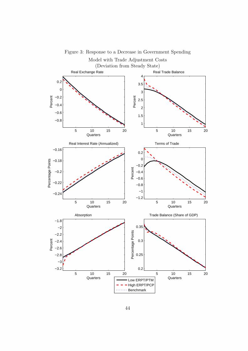
Figure 3: Response to a Decrease in Government Spending

Model with Trade Adjustment Costs(Deviation from Steady State)

5 10 15 20

−0.8

−0.6

−0.4

−0.2

0

0.2

Per

cent

Quarters

Real Exchange Rate

Low ERPT/PTMHigh ERPT/PCPBenchmark

5 10 15 20

1

1.5

2

2.5

3

3.5

4

Per

cent

Quarters

Real Trade Balance

5 10 15 20

−0.24

−0.22

−0.2

−0.18

−0.16

Per

cent

age

Poi

nts

Quarters

Real Interest Rate (Annualized)

5 10 15 20−1.2

−1

−0.8

−0.6

−0.4

−0.2

0

0.2

Per

cent

Quarters

Terms of Trade

5 10 15 20−3.2

−3

−2.8

−2.6

−2.4

−2.2

−2

−1.8

Per

cent

Quarters

Absorption

5 10 15 200.2

0.25

0.3

0.35

Per

cent

age

Poi

nts

Quarters

Trade Balance (Share of GDP)

44