Esen Erdogan-Ciftci, Eddy van Doorslaer and Ángel López-Nicolás

Does Declining Health Affect the Responsiveness of Retirement Decisions to Financial Incentives?

Discussion Paper 01/2011-005

1

Does declining health affect the responsiveness of retirement decisions to

financial incentives?

Esen Erdogan-Ciftci1 , Eddy van Doorslaer1,2 & Ángel López–Nicolás3

1 Erasmus School of Economics, Department of Applied Economics, Erasmus University Rotterdam, The Netherlands

2 Department of Health Policy and Management, Erasmus University, The Netherlands 3 Department of Economics, Universidad Politécnica de Cartagena, Cartagena, Spain.

Abstract

Both the impacts of financial incentives and health on transitions into retirement and inactivity by older workers have been studied extensively in a variety of contexts but far less is known about their interaction. Guided by the option value framework, we use Spanish data from the European Community Household Panel to compare the impact of the public pension system incentives on the retirement behaviour of workers who experienced health shocks and those who remained in good health. Our evidence suggests that the impact on retirement of forward-looking incentive measures such as the peak value is conditional on being in good health. These findings imply that many of the currently proposed and enacted pension reforms aimed at modifying financial incentives may only be effective for people in sufficiently good health.

Keywords: health, retirement, public pensions. JEL Classification: H55, I10, J26

Corresponding Author: Esen Erdogan-Ciftci Erasmus School of Economics, Erasmus University Rotterdam, PO Box 1738, 3000 DR Rotterdam, the Netherlands E-mail: erdoganc@ese.eur.nl Tel: +31-10-4088837, Fax: +31-10-4089141

Acknowledgements

This paper derives from the project “Health, Income and Work across the life cycle” funded by NETSPAR (Network for Studies on Pension, Aging and Retirement). We are grateful to Courtney van Houtven, Rob Euwals, Teresa Bago d’Uva and participants in meeting and seminars in Salamanca and Barcelona, and the Netspar Pension Workshop in The Hague, for valuable comments. Support from the Ministerio de Ciencia e Innovación through project ECO2008-06395-C05-04, co-funded by FEDER, and from Fundación Séneca through project 08646/PHCS/08 is also gratefully acknowledged.

2

1 Introduction

The relationship between health, financial incentives generated by social security systems and

labour market decisions of older workers is a salient topic of debate in OECD countries.

Decreasing mortality rates and a prolonged life expectancy have resulted in an ageing

population in general and an ageing workforce in particular. Despite substantial increases in

longevity, the labour force participation rates of the elderly have steadily fallen throughout the

twentieth century due to financial incentives encouraging early retirement and generous health

and disability insurance systems. Since these retirement arrangements seem no longer

sustainable, reforms such as capping early retirement schemes and raising the normal

retirement age have been adopted over the last decade (OECD, 2009). If increased survival

rates are associated with sufficient improvements in health during survival, then it is indeed

possible to sustain longer working lives. In this case, reforms targeting the extension of

working life through changes in financial incentives may be successful. However, workers

with poorer health may be less sensitive to such changes. This paper focuses on whether

individuals who differ in health characteristics react differently to financial incentives when

confronted with retirement decisions.

There is a body of international evidence on the importance of financial incentives and health

on retirement behaviour (Lindeboom, 2006a). However, only one paper, by Banks et al.

(2007), explicitly considers the conditionality of financial incentive effects on health status.

Examining financial incentives in the presence or absence of specific health problems for men

and women in the U.K using two waves of the English Longitudinal Survey on Aging

(ELSA), they find evidence suggesting that the (negative) impact of peak value accrual on the

odds of retirement is only significant for those without health problems. This prompts what

we will label a subordination hypothesis: financial incentives exert a stronger effect on the

chances of retirement for healthy workers. If health is poor, or in the presence of a health

shock, the financial incentives embodied in pension rules might be dampened. These financial

incentives might therefore be subordinated to health. We will discuss this hypothesis in the

context of the Option Value model (Stock and Wise, 1990; Coile and Gruber 2007) and

specify and estimate an empirical retirement model for Spain that allows us to evaluate its

merits.

3

We use data from the Spanish sample of older workers (50+) in the European Community

Household Panel (ECHP). The Spanish case is of particular interest for the purposes of this

research because in the considered period (a) the take up of private pensions was marginal,

and therefore pension wealth can be estimated from the labour market histories of workers by

simply applying the set of rules of the pay-as-you-go public system and (b) reforms enacted in

1997 introduced additional variation in pension rules. Moreover, the ECHP data contain

information that permits the construction of a health stock measure and changes therein. Our

health modeling takes into account recent insights from the literature, like the desirability of

using an indicator of health that reflects more than one dimension, as well as the need to

consider the effects of the initial health stock and its changes in order to avoid the potential

endogeneity of health in a labor outcomes equation.

The paper is organized as follows. In section 2 we review some of the recent literature on

health and retirement decisions in both the US and Europe. Section 3 discusses the interaction

of health shocks and financial incentives in the context of the Option Value model. Section 4

describes the data and our modeling strategy for financial incentives and health. Section 5

describes the econometric model and section 6 contains the discussion of its estimates. We

conclude with a discussion of the implications of our findings.

2 Health, financial incentives and retirement

The literature contains many studies about the effect of financial incentives on retirement,

among which the most well-known comparative work is reported in Gruber and Wise (2004)

which includes recent case studies for twelve countries. These applications typically find a

strong effect of financial incentives on retirement choices. For instance, in the case of Spain,

Jimenez-Martin et al. (2004)1 compute financial incentives from Social Security

administrative records and find that they exert a significant effect the probability of retirement

for private sector workers, but do not do so either for the self-employed nor public sector

workers. For Italy, Belloni and Alessi (2009) find that when employees become eligible for

pension benefits, the change in financial incentives they experience is so great that their

retirement probability increases by 30 percentage points.

1 Jimenez-Martin et al. (2004) provide a thorough description of the functioning and historical evolution of the Spanish Social Security system, from which we draw when describing and modelling the pension arrangements.

4

Surveys of early work that are on the relationship between health and retirement (e.g. Currie

and Madrian, 1999; Lindeboom, 2006a) do not discuss the conditionality of the effects of

financial incentives on health. The more recent literature has focused on the relative

importance of permanent or temporary health shocks versus a gradual deterioration of health

in retirement decisions (Bound et al. 1999; Disney et al. 2006; Hagan et al. 2008; Roberts et

al. 2010). A common finding in these studies is that changes in health play an important role

in retirement decisions, with stronger effects for the inactivity route, and that adverse health

shocks are important predictors of retirement. Lindeboom et al. (2006b) focus on the

relationship between the onset of a disabling condition and employment outcomes and

estimate that health shocks increase the likelihood of exit into the disability scheme by 138

per cent. Jiménez Martin et al. (2006) studied older Spanish workers’ labor force transitions

following a health/disability shock using cross-section data and found that the probability of

remaining in work decreases with both age and the severity of the shock, and that the

probability of remaining in employment varies substantially with the type of health condition

or disability. Another strand of the empirical literature has addressed the relative importance

of health versus financial incentives. Kerkhofs and Lindeboom (1999) investigate the effects

of health and financial incentives on three alternative exit routes in the Dutch labour market:

early retirement (ER), disability insurance (DI) and unemployment insurance (UI). They show

that health is the most important factor in explaining transitions into DI and UI schemes,

while financial incentives are dominant when explaining transitions into ER schemes. Other

papers that compare the effects of financial variables and subjective health status on

retirement are Bound (1991), Dwyer and Mitchell (1999) and McGarry (2004). They tend to

find that the effects of health are substantially stronger than those of financial incentives. In

their review article of mostly US studies, Lumsdaine and Mitchell (1999) conclude that the

impact of financial incentives on retirement is important, but can only explain half of the

observed variation in retirement rates in the US.

The studies cited above therefore suggest that the financial incentives embodied in the Social

Security rules are significant determinants of retirement. And so are poor health and health

shocks. Because health itself is obviously not directly a policy lever, the majority of policies

aimed at extending working lives focus on altering the set of pension rules - the so called

“parametric reforms” (OECD, 2009). Nonetheless, it is important to investigate whether

health might alter the effectiveness of financial incentives. That is, in addition to making

retirement more likely ceteris paribus, poor health or health shocks might dampen the

5

incentives created by such financial incentives and reforms therein. This contingency would

have interesting consequences, as it would imply that marginal reforms in pension rules will

have a limited effect on unhealthy workers. Conversely, health improvements will have not

only an independent effect on extending working lives, but they will also act through the

modification of financial incentive effects.

To the best of our knowledge, the sole study that has shed some light on this conjecture is by

Banks et al. (2007), who estimate a model for labour transitions for English workers between

age 50 and the State Pension Age in England. Their model includes measures of financial

incentives inspired by the option value model of Stock and Wise (1990), as well as different

measures of health. Interestingly, Banks et al (2007) find that peak value accrual –an

incentive measure capturing the cost of opportunity of retiring today in terms of foregone

future pension benefits- only exerts a significant effect on the likelihood of retirement for

those in good health.

In the following section we provide a discussion of how health shocks are likely to influence

the effect of the financial incentives embodied in the Option Value model of retirement. In

subsequent sections we will specify and estimate an econometric model that nests the

possibility that the effects on retirement of such financial effects vary with health.

3 Health shocks and retirement in the Option Value model

There is a considerable body of literature on the relationship between social security benefits

and labor force participation (for a review, see Coile and Gruber, 2007). For retirement, Stock

and Wise (1990) emphasized the trade off between the level of retirement benefits and the

entire future potential income and wealth stream from working. Their option value (OV)

model main insight is that retirement models should consider explicitly the utility difference

between retiring today and retiring at the date that optimizes utility.

Coile and Gruber (2007) have provided an empirical implementation of the OV model where

individuals compare the value of retiring immediately with the value of continuing work and

holding the option of retiring in the future. Individuals at work re-evaluate this comparison at

6

each period. For our purposes, we consider what the effects of health shocks and their

interactions with financial incentives are in the context of such a model.

Suppose individual i will receive wage income sY in year s as long as he continues to work.

If the individual retires in year s, he will receive retirement benefits sB . If we define R as the

year of retirement, and benefits as )(RBs , then the value of retiring at R is given by:

∑ ∑−

= =

−− +=1

))(()()(R

ts

T

Rs

s

ts

tss

ts

tst RBUYURV βρβρ (1)

where β is a subjective discount factor and ts

ρ is the probability of being alive at some

future date conditional on being alive today. Coile and Gruber (2007) assume that the

individual indirectly derives utility from real income while working, )( sYU = γsY and utility

from pension benefits received while retired γ)]([))(( RkBRBU ss = where k is a parameter

to account for disutility of labor and γ is a parameter of risk aversion. The OV model

assumes that in every period t, individuals compare the lifetime utility of retiring at time t

with the lifetime utility of retiring at a future “optimal” date, R*, the retirement date at which

lifetime utility is maximized. That is, the individual evaluates

T}1,...,{t R with)(max solves * R where; )(*)( +∈−= RVtVRVOV tttt (2)

Therefore, the OV at time t is:

∑∑ ∑=

−−

= =

−−

+=

T

ts

s

ts

ts

R

ts

T

Rs

s

ts

tss

ts

tst tkBRkBYOV γγ βρβρβρ γ))(( - *))(()(

1*

*

(3)

which equals labour income up to R*-1, plus benefits accruing from R* conditional on having

retired at R*, minus the benefits that would have accrued from the current period up to T if

retirement was chosen contemporaneously. If, for any future date R*, OV is still positive, the

individual will continue working. If not, he will retire. So, the higher the OV, the lower the

probability of retiring.

7

It is useful to rewrite Equation 3 as the sum of the following three summands:

∑∑∑−

=

−

=

−−

=

−

−+=

1*

*

1*

))(( -]))((*))([()(R

ts

s

ts

ts

T

Rs

ss

ts

ts

R

ts

s

ts

tst tkBtkBRkBYOV γγγ βρβρβρ γ

(4)

The first summand measures labour income until R*. Defining Pension wealth as the expected

present value of a worker’s stream of pension benefits at year t, should he retire at a given age

h2;

)),((),( hsBEthPWT

hs

t

ts

ts∑=

−= βρ (5)

where )h,s(BE t is the pension expected at age s ≥ h in case of retirement at age h. We can

easily see that the third summand is a measure of pension related financial incentives: i.e.

(lost) “pension wealth” from not retiring until R*.

The second summand in Equation 4 (between brackets) measures the “peak value” at R*.

Given PW, the peak value (PV) is defined as the maximum difference in PW between retiring

today and retiring at the age at which the expected value of the PW is maximized3:

RthPWPWPV thht ,...,1 },{max +=−= (6)

Equation 4 allows us to discuss the effects of income, growth of benefits, pension wealth and

health shocks in the context of the OV model. From this equation we can see that, ceteris

paribus, higher income will increase OVt and therefore make retirement less likely. The

second summand shows that the growth of benefits with a longer active life - as proxied by

the peak value - will raise OVt and make retirement less likely: the greater the difference

between brackets, the more likely that the OV expression is positive. Finally, the third

summand enters with a negative sign: the greater the lost pension wealth (as explained earlier,

the sum of benefits in the third summand is the pension wealth that would be obtained

between time t and R*), the lower OVt, and the more likely it is to retire at time t.

2 T is assumed to be 100 and the discount factor to be 0.95238 ( discount rate of 5 percent) in the empirical analysis. 3 In the computation of pension wealth,R is a mandatory retirement age (which does not exist in Spain), but we have assumed that R=70.

8

There are several ways through which a health shock can affect the individual’s evaluation of

future OVs. One is a direct effect on the future string of labour income, which may be

reduced if the shock affects productivity. But this is not our main concern here. We are

interested in the indirect effects that are channeled through the parameters that determine the

peak value and pension wealth. A second possible effect, for instance, is an increase in the

marginal disutility of labour by an increase in the parameter k in the model. A third effect is a

possible update (downward adjustment) of the survival probabilities tρ . Finally, a health

shock might also raise the time preference rate of the individual, and reduce the discount

factor β . In this sense, it would reduce the value of future consumption to the individual and

act in the same direction as the downward adjustment in survival probabilities.

First, consider the effect of a health shock on pension wealth (third summand in Equation 3).

A health shock increases the disutility of labor (k). An increase in k boosts the value of the

string of benefits and, via the effect of this summand, reduces future OVs. However, a health

shock may also result in a reduction in the survival probabilities or an increase in time

preference, and this will have a compensating effect. Therefore, the net effect of a health

shock, ceteris paribus, on pension wealth is indeterminate and we cannot expect a priori the

interaction of health shock with pension wealth to go in either direction.

There is also no a priori theoretical expectation on the sign of the interaction of health shocks

with the peak value. Through the second summand in Equation (4), the increase in k would

act in the direction of increasing future OVs (thereby reducing the chances of retirement),

while the decrease in survival probabilities acts in the opposite direction (increasing the

chances of retirement).

Notwithstanding the theoretical indeterminacy of the impact of a health shock on the effects

of peak value and pension wealth on the likelihood of retirement, the OV model suggests that

the effects of an increase in the disutility of labour are more likely to prevail in summands

corresponding to near future periods than in those corresponding to the distant future. This is

a consequence of the fact that survival probabilities and discount factors will in the limit drive

the summands towards zero, and even more so after a health shock. In consequence, while we

cannot rule out the possibility that a health shock alters the chances of retirement in the same

direction through its impact on peak value and pension wealth, it is a priori more likely that

9

such a coincidence, if it exists, manifests itself in a shock which makes pension wealth more

inciting to retirement and peak value less inciting to continue working rather than the opposite

(i.e. pension wealth less inciting to retirement and peak value more inciting to continue

working).

Whether and by how much health alters the effects of financial incentives created by pension

rules are therefore empirical questions, as far as the OV model can predict. A hypothesis of

subordination of financial incentives to health, stating that some or all of the effects of the

financial incentives embodied in pension rules might be dampened by poor health or health

shocks, is therefore plausible. Indeed the results of Banks et al. (2007) would seem to confirm

such a hypothesis for the case of the peak value. In the following sections we will investigate

this empirically using data from the Spanish labour market.

4 Data and variables

4.1 Data

Our data are taken from the public use files of the European Community Household Panel

(ECHP). The ECHP was designed and coordinated by Eurostat, the European Statistical

Office and consists of a longitudinal survey based on a standardised questionnaire that

involves annual interviewing of a representative panel of households and individuals 16 years

and older in each EU member state. It includes respondents’ demographic background,

employment status, income, health status, social transfers etc. We make use of all eight waves

available (1994-2001) for Spain. Self-reported labour market status is defined as ‘employed’

if the respondent is working full-time or part-time in paid employment, and ‘self-employed’ if

in self-employment or working in a family enterprise. Old-age retirement status is also based

on self-reports. In line with a number of other studies (e.g. Bound et al. 1999; Disney et al.

2006; Hagan et al. 2008), we also use two retirement definitions: (i) the narrowly defined

retirement status, corresponding to a self reported retirement and (ii) an extended definition

including, in addition, being reported as economically inactive and doing housework, but

excluding those reporting themselves as unemployed. Retirement is taken as an absorbing or

permanent state and any subsequent transitions back to work are ignored. We will refer to

10

these two labour outcomes as “standard retirement” and “extended retirement” throughout the

paper.

We apply the stock sample method (Lancaster, 1990) and follow all individuals who are in

employment (either employed or self employed) and in the age group 50-64 in the first wave,

over a period when they are at a risk of retiring. These individuals can stay in the labor force,

retire or be lost to follow up. Transitions into other states as well as attrition are summarized

in Table 1. The initial stock sample consists of 1449 employed individuals, 74% male, and

46.3. %, 32.9% and 20.7% in age groups 50-54, 55-59 and 60-64 respectively. The stock

sample gradually reduces to 347 by the eighth wave, while the number of self-reported retired

respondents increases from 42 in wave 2 to 302 in wave 8.

{Insert Table 1 here}

The main income variable used is the log of total household income. Other socio-

demographic variables used in the analysis include: house ownership, educational attainment

graded using the highest grade of education achieved on the 3 level ISCED scale - completed

third level secondary education; completed second stage of secondary education; completed

less than second stage of secondary education; a quadratic function of age; whether children

under 12 living in the household; and whether the individual is married. Names and

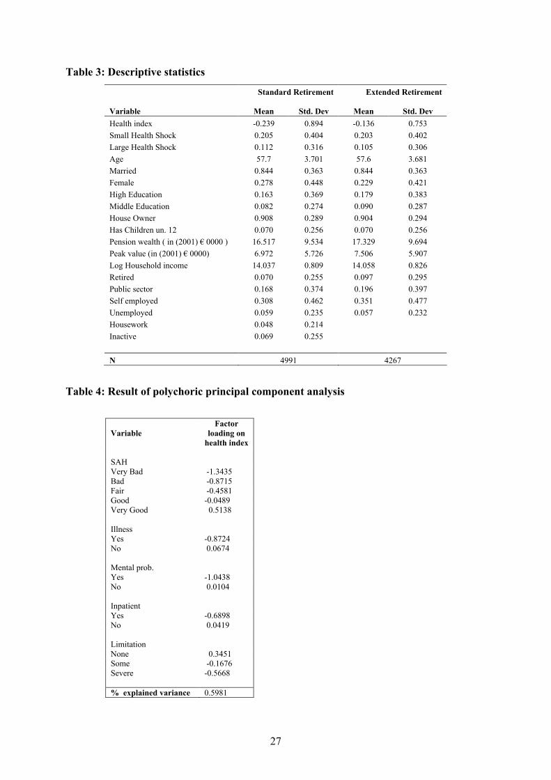
definitions of variables and their descriptives are presented in Tables 2 and 3 for the

estimation samples for both definitions of retirement.

{Insert Table 2 & Table 3 here}

4.2 Modelling pension incentives

Spain has a mandatory pay-as-you go public pension system run by the Social Security. For

the average Spanish person, receiving a pension usually means receiving a public pension, as

less than 1% percent of Spanish retirees draw more than 10% percent of their annual income

from a private pension plan. In addition, the Social Security system offers unemployment

benefits, disability benefits and some non-contributory benefits. We will focus on

contributory public pension benefits. These are not directly observable in the ECHP.

However, we are able to reconstruct them by exploiting information on individual labour

11

histories, upon which we apply the set of rules governing benefits, penalizations for early

retirement etc. The measures of pension wealth thus obtained incorporate variation from three

sources. First, there are several Social Security regimes, each with different rules. Secondly,

there is individual variation in the length and size of contributions to the corresponding

regime. Finally, in 1997, a year covered by our data set, there was a reform in pension rules

that affected some of the Social Security regimes. 4 While the first two sources of variation

cannot be considered strictly exogenous to retirement, the dependence of contemporaneous

pension wealth on decisions taken long ago (i.e. which Social Security regime) and on the

history of contributions over a relatively long period guarantee that pension wealth is

predetermined. The additional variation afforded by the 1997 reform can be considered

exogenous.

Public contributory pensions are provided by the following three programs in Spain: (1) the

“General Social Security Scheme” (Regimen General de la Seguridad Social, or RGSS) is the

“default” regime for private sector employees but it also covers the members of cooperative

firms, the employees of most public administrations other than the central governments and

all unemployed individuals complying with the minimum number of contributory years when

reaching 65; (2) the “Special Social Security Schemes” (Regimenes Especiales de la

Seguridad Social, or RESS) covers the self-employed and professionals plus some groups of

workers in certain occupations. The RESS includes five special schemes, but by far the largest

is the one for the self employed (RETA); and (3) the scheme for government employees

(Regimen de Clases Pasivas, or RCP) includes public servants employed by the central

government and its local branches.

For each of the defined pension schemes in the Spanish social security system, we compute

pension wealth and the peak value which, as defined in section 3, captures the trade off

between retiring today and working until a year with a higher PW. Retirement incentives

differ considerably across the three groups, as is illustrated for three prototypical individuals

in Figure 1 (Also see Appendix Part-2 for details on the estimation of pension incentives by

age). Figure 1 presents pension wealth profiles for a man who is fifty years old in 1994 and

has the following characteristics: a) Profile pwrgss50: affiliated to RGSS regime, has worked

since age 15, earns 12000 Euros a year, receives salary increases in line with inflation, has

4 The detailed description of this reform and changes in the rules which effects eligibility and amounts can be found in Appendix -Part 1.

12

normal retirement age at 65, but can retire at age 60 with a penalty (b) Profile pwreta50:

affiliated to RETA regime, same characteristics as the individual in Profile pwrgss50, (c)

Profile pwrgcp50: RCP regime, same characteristics as the other two profiles, but early

retirement is possible at age 60 without any penalty since he has been working more than 30

years.

{Insert Figure 1 here}

Before the age of 65 (age 60 for RCP), pension wealth increases because both the benefit base

and replacement rate are rising (while the total number of periods that the worker receives a

pension in the computation of pension wealth falls, the increase in benefit base and

replacement rate is sufficient to compensate for this decrease). However, after age 65, the

replacement rate is constant and although the benefit base is increasing, this does not suffice

to compensate for the decrease in the remaining expected life span. Moreover, additional

years of work add nothing to the expected pension amount and, as a result, pension wealth

after age 65 decreases. Whether or not pension wealth increases depends on whether the rise

in pension income from delaying retirement is sufficient to outweigh the fact that the pension

would be received for one fewer year. In all three schemes, individuals are financially

penalized for leaving prior to normal retirement age. There is typically no bonus for

remaining in the scheme beyond the normal retirement age.

The patterns of pension wealth for the RETA and RGSS schemes are very similar. The RCP

individual turns 60 in 2004, and has worked for more than 30 years, so he can retire with full

pension in 2004. As a result, his profile peaks at age 60. Pension wealth in the RCP scheme is

higher than in the private sector due to differing rules for civil servants. Their benefit base is

higher than in other regimes and the replacement rate increases irregularly with seniority.

While the rules are identical for RETA and the RGSS, their covered earnings are computed

differently. The pension wealth profile is higher for RETA than for RGSS, because the legal

minimum earnings in pension formulae applicable to RETA workers are higher than for

RGSS workers. This rule attempts to neutralise the tendency for self employed workers to

underreport their income.

In addition to the computed pension wealth and financial incentives measures, we created

three dummy variables indicating when the person could start drawing pension benefits:

13

“public pension entitled after two periods” indicates that the person will not be able to draw

pension benefits until at least two periods [ 0),2( & 0),( >+= hsBhsB ]; “public pension

entitled in next period” indicates that the respondent will be able to draw a pension from the

next year [ 0)h,1s(B & 0)h,s(B >+= ]; finally, the dummy variable “public pension

entitled this period” indicates the person is able to draw benefits currently or at some point

during the current year [ 0)h,s(B > ].

4.3 Measurement of health stock and health shocks

The relationship between observed and “true” measures of health has been a permanent

concern for researchers. For lack of more objective data on health, most previous studies have

used self-assessed health or other subjective reports of health limitations. This entails obvious

potential problems of accuracy, endogeneity and justification bias in retirement and labour

market transition models. Many recent studies have attempted to deal with these problems by

constructing an underlying “health stock” for each individual and tracking longitudinal

changes in this measure as a proxy for individual “health shocks”. (Bound et al. 1999, Disney

et al. 2006, Hagan et al. 2008, Roberts et al. 2010). The latent health measure is then obtained

as the predicted value of SAH, using supposedly more objective self-reported health

indicators related to specific medical conditions and functional limitations as predictors. This

is analogous to using the health indicators as instruments to ‘purge’ the measurement error

from the SAH variable. This, of course, implicitly assumes that (i) SAH is the true variable

belonging in the labor supply model and that (ii) the instruments can be legitimately excluded

from such equation. While these “instruments” can be argued to be more objective self-

reported measures of health than the usual five category SAH scale, it is not clear that they are

valid instruments, in the sense that they cannot be argued to be entirely free from justification

bias or measurement error themselves (Thomas and Frankenberg, 2002).

Our approach is based on the recognition that while some self reported variables might be

more objective than others, there is no single health variable in the ECHP (or any other

similar survey) that can be considered the true health variable belonging in a labour outcomes

model. All of these variables can only be considered indicators of true health, each capturing a

different dimension of underlying unobservable health. In this sense there is an argument for

not dismissing potentially useful information by opting for one or another variable as the

14

“right” one for the model. Therefore, we construct a single health indicator combining

information from all health related variables included in the ECHP. This indicator can be

thought of as a proxy variable for true unobservable health. Even if we were imperfectly

proxying true health, the magnitude of the bias on the other explanatory variables in the

retirement equation is smaller than if observed health were omitted. In addition, we still

obtain the right sign on the effect of health (Wooldridge, 2002). Nothing prevents this proxy,

of course, from being correlated with the error term in a labour transitions equation. In

particular, there could be justification bias (an unobservable preference for leisure might be

correlated with our index) or simultaneity bias. Fortunately, the longitudinal nature of our

dataset allows us to both address the issue of simultaneity (by using predetermined values for

health) and to model unobserved fixed effects.

The choice of health indicators from the ECHP consists of a set of self reported health

measures relating to limitation in daily activities, recent illness or mental problems and the

history of in-patient hospital episodes. The definitions of the five variables used in the

analysis are: (i) How do you rate your health in general? (SAH) (5 categories, very good to

very bad); (ii) Are you hampered in your daily activities by any physical or mental problem,

illness or disability? (3 categories; severely, to some extent, no); (iii) During the past two

weeks, have you had to cut down things you usually do about the house, at work or free time

because of illness or injury? (Yes/No); (iv) During the past two weeks, have you had to cut

down things you usually do about the house, at work or free time because of an emotional or

mental problem? (Yes/no); (v) During the past 12 months, have you stayed at least one night

in a hospital? (Yes/no).

Because these health indicators are measured on ordinal or binary scales, which violate the

standard multivariate normality assumptions, we use polychoric principal components

analysis (PCA).5 The resulting index of latent health is a linear combination of the observable

health-related variables. Table 4 presents the factor loadings of the observed variables used on

our synthetic indicator of good health. It can be seen that the index is mostly driven by the

“very poor” and “poor” categories of self-assessed health, by the “severe” category of health

limitations, by the reporting of an illness or a mental health problem, and by the reporting of

5 Kolenikov and Angeles (2004, 2009) used a Monte Carlo simulation to show that failure to control for discreteness in variables leads to significantly inferior results. The standard PCA approach, especially when dummy variables are constructed from ordinal variables, has lower explained variance than the polychoric approach.

15

an inpatient hospital episode. Most health variables contribute substantially to the constructed

health index, with the highest scores for self-reported health and mental health problems.

{Insert Table 4 here}

The identification of negative health shocks offers a convenient way to eliminate a potential

source of endogeneity bias caused by the correlation between individual-specific unobserved

characteristics and health when the decision to retire may be related to a “health shock” i.e. a

sudden sharp health deterioration (Disney et al., 2006). Our two measures of health shock are

based on the differences between two consecutive waves in an individual’s latent health index

value.6 We created two binary indicators: a “small health shock” for a decrement of less than

one standard deviation and a “large health shock” for a decrement of one or more standard

deviations. This is similar to the concept of an acute health shock as used by Riphahn (1999).

Table 5 shows that deterioration in health is accompanied by the occurrence of both types of

health shocks. Their prevalence increased across waves, occurring in 29.61 % of individual’s

in wave 2 and in 32.74 % in wave 8.

{Insert Table 5 here}

5 Models and estimation

Stock samples are sometimes used to estimate models of duration, because the start of the

observation period usually coincides with the start of some natural measure of time at risk. In

the case of transitions to retirement, this event can be interpreted as a “failure” in the jargon of

duration models.7 An advantage of the stock sampling approach with discrete time data, like

ours, is that retirement decisions can be modelled as the probability that an individual reports

“failure” in the next period. This method represents the transition to retirement as a discrete

time hazard model. Conditioning on stock sampling ―so that the time periods prior to

6 As a robustness check we also implemented the Bound (1991) and Kerkhofs and Lindeboom (1995) approaches to address issues associated with measurement error in SAH. This basically involves predicting SAH as a function of more ‘objective’ measures of health to define a latent health stock variable. We adopt an ordered probit (OP) and generalised order probit (GOP) model to allow for different thresholds when reporting SAH. Using these alternative health stock measures in the retirement models, we found the effects of health stock and health shocks to be very close in size and significance to our PCA based approach. 7 Recent examples with time discrete data include Disney et al. (2006), Hagan et al. (2008), and Roberts et al. (2010).

16

selection into the stock sample can be ignored― the estimation of our discrete time hazard

model is simplified and a binary outcome estimation method (retired versus not retired)

becomes appropriate.8

For each year, we create an indicator for transition into retirement (and extended retirement),

and estimate a random effects probit regression of this transition on a number of independent

variables, including the initial value of the health index in wave 1, health shocks, financial

incentives, age (in quadratic form), indicators for educational attainment and type of job,

labor earnings, and other individual characteristics. We condition on the initial value of the

health index to account for any other aspects of health potentially correlated with retirement

and/or unobserved effects as well as health shocks to ensure that all the health variables in the

retirement transition equation are predetermined. Formally, we adopt the following binary

outcome panel data model for the two definitions of retirement considered in this paper.

e otherwis , and if r r

,...,T,...,n , t iεβxηsµh)hh λαr

*

i,ti,t

i,tititiit i,t i

*

i,t

0 01

11(

11

1111

>=

==++++−+=

++

+++ (7)

where *1 ti,r + is the latent propensity for individual i to report retirement in the next year, ith is

the health stock and i1h is initial health stock in wave 1 , its is a vector containing peak value

and pension wealth, itx is a vector of predictors including socio-demographic and socio-

economic characteristics and iα is an individual specific, time-invariant random component.

itε is a time and individual-specific error term which is assumed to be normally distributed

and uncorrelated across individuals and waves. itε is assumed to be strictly exogenous; that

is, the itx , ith and its are uncorrelated with isε for all t and s.

A well-known limitation of the standard random effects model is that it assumes iα to be

uncorrelated with the explanatory variables. There are grounds to suspect that this assumption

may not hold in our case. For instance, the individual effect could be picking up a preference

for leisure, and we can expect this to be correlated with reported health indicators

8 Jenkins (1995) shows that in such cases models for binary dependent variables (like probit, logistic and complementary log-log) can be used to model discrete time hazard functions.

17

(justification bias). We address this limitation by parameterizing the individual effect as a

function of the time means of a subset of the regressors (Mundlak, 1978; Chamberlain, 1984;

Wooldridge, 2002). We implement this so-called Mundlak specification by parameterizing the

distribution of the individual effects as:

)N(0, x 2 i σα ~uu iii += (8)

where ix is the within individual mean or a combination of leads and lags of the regressors.

In terms of implementation, this simply has the effect of adding time means or lags and leads

to the set of explanatory variables. iu is assumed to be distributed )N(0, 2σ independent of

the x variables and the idiosyncratic error term itε . Substituting equation (8) into equation (7)

gives a model that maintains a random effects structure, in the sense that the composite error

term is the sum of an individual time-invariant term ( iu ) plus a pure white noise term ( itε ),

but where the maintained assumption of independence between the former and the regressors

is more reasonable.

To assess whether financial incentive effects for retirement differ when the worker has

suffered a health shock, we also introduce interaction terms between the health shocks and the

financial incentives variables. When dealing with non-linear models, the interpretation of ―

and inference on ― interaction terms require special attention (cf. Ai and Norton, 2003;

Mullahy, 2008)). First, the partial effect of an interaction term could be non-zero even if the

directly estimated coefficient of the interaction term is zero. Second, we cannot rely on

standard tests on the coefficients of the interaction term to test the statistical significance of

the interaction effect. Third, the interaction effect is conditional on the independent variables

and may have different signs for different values of the covariates. Therefore, to determine the

magnitude of the interaction effects, it is necessary to compute the cross derivative (for

continuous variables) or differences (for categorical ones). We used a bootstrapping

procedure to obtain standard errors for the interaction terms.

18

6 Results

Table 6 presents the marginal effect estimates for both definitions of retirement, standard and

extended. As explained earlier, our specification allows for correlated individual effects, the

latter specified as linear functions of within-individual means of observables, as proposed by

Mundlak. This specification was preferred over a standard random effects specification on the

basis of a test that rejects the null of joint insignificance of the terms in the non-stochastic part

of Equation 8 (labeled “Mundlak averages” in Table 6). Further tests suggested that these

terms should include the means of health shocks, pension wealth, labour status dummies,

household income and marital status.

Before examining the parameter estimates, it is useful to note that the unconditional

probability for retirement (extended retirement) is 6.4% (9.1%). Our results show that, as

expected, healthier workers are less likely to retire: the initial level of health shows a strong

and significant negative effect on the probability of retirement in both models. Indeed,

workers whose health stock is one standard deviation below the mean are 1% (2%) more

likely to enter into retirement (extended retirement). The health shock effects also differ

across the two definitions of retirement. Neither of the shocks - small or large - shows any

significant effect on standard retirement. For the extended definition of retirement, however,

the occurrence of a large health shock does significantly increase the probability of retiring by

about 6 percentage points.

{Insert Table 6 here}

We find the expected effects for our measures of financial incentives: a significant positive

effect for pension wealth and a significant negative effect for peak value. Greater expected

pension wealth increases the odds of retirement, while a financial reward to delaying

retirement, in the form of a higher benefit level, increases the chances of continuing to work.

Pension wealth can be interpreted as an income effect, which is consistent with the idea that

leisure is a normal good. Pension accruals (or their peak values) are sometimes interpreted as

“price effects”, as they reflect the relative cost, in terms of pension wealth, of not delaying

retirement, and our estimates show a significant effect in the expected direction. The size of

the impact is greater for pension wealth: while the elasticity of the odds of retirement with

respect to pension wealth is 2.68 (2.33 in the model for extended retirement), that with respect

19

to peak value is -0.272 (-0.518 in the model for extended retirement). Another way to express

the effect of these financial incentives is by considering the impact on the probability of

retirement of a hypothetical increase in pension wealth or peak value. For instance, 10,000 €

of additional pension wealth (about 6% of the average pension wealth in our sample) raises

the probability of retirement by 1% (1.2% in the model for extended retirement). An

equivalent increase in peak value (in this case amounting to 14% of the average peak value in

the sample) decreases the probability of retirement by 0.25% (0.63% in the model for

extended retirement).9

The two variables indicating the time of entitlement to a public pension are strongly

significant in the standard retirement model (amounting to an increase of 2.5% or 4.6% in the

odds of retirement for those who can start drawing benefits either in the current year or during

next year), but not in the extended retirement model. These results confirm that, even when

controlling for pension wealth, people closer to the age of being able to draw pension benefits

are more likely to retire than those who will not be able to draw such benefits for at least two

more years. This raises some interesting questions about the potential presence of liquidity

constraints (or illiquidity aversion).

For other covariates, we find that higher income reduces the likelihood of both types of

retirement. While this is consistent with the predictions of the OV model, as exposed earlier,

the effect is small in magnitude, as the elasticity with respect to household income is -0.14 (-

0.10 in the extended retirement model). The quadratic function of age we use shows that the

rise in the retirement probability increases with age10, for both measures of retirement. Ceteris

paribus, women are significantly more likely to leave the labor market (through the extended

retirement route)11. The exit likelihood also differs by type of job. The self-employed are less

likely to retire, ceteris paribus, whereas the unemployed are more likely to retire in

comparison to those employed. Public sector employees are less likely to retire than those in

the private sector. Being a house owner increases the probability of retirement in both models.

Married and individuals who have children are less likely to retire. All remaining covariates

9 Belloni and Alessie (2009), in the context of a comparable theoretical and empirical specification for the retirement decisions of Italian workers, find that increasing pension wealth by 10000 € would increase the odds of retirement by 0.095%. The corresponding figure for 10000 worth of extra peak value is a reduction of 1% in the probability of retirement. 10 We tested for a cubic polynomial in age in some specifications but the cubic term was never significant. 11 As a robustness check, we included interaction terms between female and financial incentives and health variables, but did not find any significant gender differences in retirement effects.

20

were insignificant in both retirement models. While the coefficients of the Mundlak averaged

terms capture the correlation between covariates and the individual unobserved effect, there is

no clear economic interpretation of their contribution.

We now focus on the interactions between health shocks and financial incentives. In

particular, we examine whether the effects of pension wealth and peak value differ between

workers in good health (i.e. who do not incur a health shock) and those in poor health (who do

incur a health shock). Starting with the standard retirement model, we find that the marginal

effects associated with the interaction of peak value with the occurrence of a large or a small

health shock (estimated at 0.0045 and 0.0035 respectively) fully counteract the stand-alone

marginal effects of peak value (estimated at -0.0025) on the retirement probability. This

means that the small (elasticity of -0.272) but significant negative effect of peak value on the

odds of retirement vanishes for workers who have endured a health shock. In the case of

extended retirement, we find that the elasticity of peak value is halved (from -0.518 to -0.222)

for those who experienced a small health shock. In contrast, the estimate for the interaction of

peak value with a large shock in this model is insignificant and has a smaller order of

magnitude.

In the case of the interaction of pension wealth with the occurrence of health shocks, we find

that small shocks increase by a statistically significant amount the average marginal effect of

pension wealth, although the size of such increase relative to the main effect is small,

especially in the case of standard retirement. The corresponding elasticity increases from 2.68

to 3.45 (2.33 to 2.86 in the model for extended retirement). On the other hand, larger health

shocks do not appear to exert a significant impact on the pension wealth marginal effects of

either model.

Overall we find evidence suggesting that health shocks do have an impact on the effects of the

financial incentives embodied in pension rules. Although these impacts are relatively small in

absolute value in the case of pension wealth, they contribute to reinforcing its main effect of

making retirement more likely. Moreover, health shocks have a relatively large impact on the

effects of peak value. In the case of standard retirement in particular, we find that the full

effect of peak value vanishes among workers who have endured a health shock, regardless of

whether it is a large or a small one. Our estimates therefore suggest that health shocks impact

on the effects of financial incentives in the same direction: exacerbating the positive effect of

21

pension wealth on the chances of retirement and dampening the negative effect of peak value

on the chances of retirement. This is consistent with the a priori expectation that we have

expressed in Section 3: despite the impossibility to predict the direction of the effects of

health shocks on the chances of retirement through their impact on peak value and pension

wealth, it is likely that a shock makes pension wealth more inciting to retirement and peak

value less inciting to continue working.

7 Conclusion and discussion

Our study investigates the role played by health shocks, the financial incentives generated by

pension schemes and their interaction in retirement decisions of older workers. In the context

of an empirical version of the Option Value model, we explore the effect of health shocks on

standard measures of financial incentives and pose a subordination hypothesis: the effects on

the probability of retirement of forward looking financial incentives differ according to

whether workers have suffered a health shock. Our theoretical discussion also suggests that ―

although other patterns for the impact of health shocks on such effects cannot be ruled out ―

it is likely that a shock makes pension wealth more inciting to retirement and peak value less

inciting to continue working.

We test these conjectures using data from the Spanish sample of the ECHP, with which we

estimate models for two definitions of retirement ―both old age standard retirement and an

extended definition including inactivity- using empirical measures of health stock, health

shocks, and financial incentives of the pension system. Our estimates show, in line with

existing studies, that the stock of health is an important predictor of retirement. Also in line

with theoretical predictions and existing estimates, we find that pension wealth increases the

chances of retirement (elasticities of 2.68 and 2.33 for standard and extended retirement

respectively) and peak value reduces the chances of retirement (elasticities of -0.272 and -

0.518).

Our results show support for our subordination hypothesis: health shocks make pension

wealth more inciting to retirement and peak value less inciting to continue working. While the

size of the impact on the elasticity of retirement with respect to pension wealth is small in

relative terms (a change from 2.68 to 3.45 in the model for standard retirement), health shocks

22

completely wipe out the effect of peak value. This finding is in line with the results in Banks

et al. (2007) who found the (negative) impact of peak value accrual on retirement to be

significant only for those without health problems.

Our results have some interesting implications for the recent reforms of public pensions in

Spain, where measures aimed at delaying retirement were enacted in 2007. These operate

primarily through increases in the pension accruals after age 65, the statutory age of

retirement for most workers. Under the new rules, employees that continue working beyond

the age of 65 will see the value of their state pension benefits increased by 2% per full year of

work up until the age of 70 years.12 But given the low elasticity of retirement to peak value

that we have estimated, it is expected that such measures will have little effect on delaying

retirement. Moreover, our results suggest that these measures will be completely ineffective

for workers who experience a health shock.

The poor state of public finances in Spain after the financial meltdown of the late 00’s is

prompting further reforms to the pension system. By early 2011, the government and the trade

unions are bargaining over the possibility of raising the statutory age of retirement to 67. Our

estimates suggest that such reform is likely to be more effective at delaying retirement, as one

of the strongest explanatory variables in our models is the possibility to start drawing pension

benefits.

To sum up, our findings highlight an important point: marginal changes to the financial

incentives in pension systems will achieve less in terms of keeping older workers at work if

these people are unable to respond to the incentives because of health problems. Therefore,

such policies are to be considered in conjunction with appropriate health policies to contribute

to the target of keeping older workers active for longer. This suggests that a potentially

fruitful avenue for delaying retirement decisions would be to minimize the direct costs of

working for individuals with some health deterioration. Technological advances that offer the

possibility to work flexible hours and/or work from home should be exploited to their

maximum potential in this sense. There is, finally, a positive message for the sustainability of

12 Also, if an employee has contributed to the pension scheme for 40 years by the time they reach the age of 65,

they will receive a higher annual increase of 3% of their benefits value (LEY 40/2007, de 4 de diciembre, de

medidas en materia de Seguridad Social).

23

the public pension system coming from the estimated effect of health. At face value our

results suggest that a better health level does, ceteris paribus, reduce the likelihood of

retirement. If technological progress and rising living conditions are to improve the average

level of health, we should, ceteris paribus again, expect a reduction in the odds of retirement

at any age. Of course, these gains –as far as sustainability is concerned- may be countered by

other factors. An increase in the value of leisure, perhaps induced by higher levels of income,

could well have larger effects than the likely effect of health improvement. We leave these

issues for the future research agenda.

8 References

Ai C. and Norton E.C. (2003). Interaction terms in logit and probit models. Economic Letters

80; 123-129.

Banks J., Emmerson C. and Tetlow G. (2007). Healthy retirement or unhealthy inactivity:

how important are financial incentives in explaining retirement? The Institute for Fiscal

Studies Working Paper. London.

Belloni M. and Alessie R. (2009). The importance of financial incentives on retirement

choices: New evidence for Italy. Labour Economics 16; 578–588.

Bound J. (1991). Self-reported versus Objective measures of Health in Retirement Models.

Journal of Human Resources 26; 106-138.

Bound J., Schoenbaum M., Stinebrickner T. and Waidman T. (1999). The Dynamic Effects of

health on the labour force transition of older workers. Labour Economics 6; 179-2002.

Chamberlain G. (1984). Panel data. In Handbook of Econometrics, Vol. 1, Griliches Z,

Intriligator MD (eds). North Holland, Amsterdam, 1247–1318.

Coile C. and Gruber J. (2007). Future Social Security Entitlements and the Retirement

Decision. The Review of Economics and Statistics 89(2); 234-246.

Currie J. and Madrian B. (1999). Health, Health Insurance and Labour Market in Handbook

of Labour Economics; Volume 3C, Amsterdam; New York and Oxford: Elsevier Science,

North Holland, 3309-3416.

Disney R., Emmerson C., and Wakefield M. (2006). Ill health and retirement in Britain: A

panel data-based analysis. Journal of Health Economics 25; 621-649.

Dwyer D.S. and Mitchell O.S. (1999). Health Problems as determinants of retirement: Are

self-rated measures endogenous? Journal of Health Economics 18; 173-193.

24

Gruber J. and Wise David A. (2004). Social Security Programs and Retirement around the

World: Micro-Estimation. The University of Chicago Press, Chicago, IL.

Hagan R., Jones A.M. and Rice N. (2008). Health shocks and the hazard rate of early

retirement in the ECHP. Swiss Journal of Economics and Statistics 144; 323-335.

Jenkins S.P. (1995). Easy estimation methods for discrete-time duration models. Oxford

Bulletin of Economics and Statistics 57(1); 129-138.

Jimenez Martin S., Boldrin M. and Peracchi F. (2004). Micro-modelling of Social Security

and Retirement in Spain", in Gruber, J. and Wise, D. Social Security Programs and

Retirement around the World: micro estimation. The University of Chicago Press, Chicago,

IL.

Jimenez Martin S., Labeaga J.M. and Vilaplana Prieto C. (2006). A sequential model of older

workers' labor force transitions after a health shock. Health Economics 15; 1033 - 1054.

Kerkhofs M. and Lindeboom M. (1995). Subjective Health Measures and State Dependent

Reporting Errors. Health Economics 4; 221-35.

Kerkhofs M. and Lindeboom M. (1999). Retirement, Financial Incentives and Health. Journal

of Labour Economics 6; 203-227.

Kolenikov S. and Angeles G. (2004). The Use of Discrete Data in Principal Component

Analysis with Applications to Socio-Economic Indices; CPC/MEASURE Working paper No:

04-85.

Kolenikov S. and Angeles G. (2009). Socioeconomic status measurement with discrete proxy

variables: Is principal component analysis a reliable answer? Review of Income and Wealth

55(1); 128 – 165.

Lancaster T. (1990). The econometric analysis of transition data. Cambridge: Cambridge

University Press.

Lindeboom M. (2006a). Health and work of older workers. In Elgar Companion to Health

Economics; Jones AM (ed). Edward Elgar: Aldershot.

Lindeboom M., Llena Nozal A. and van der Klaauw B. (2006b). Disability and Work: The

Role of Health Shocks and Childhood Circumstances. Tinbergen Institute Discussion Paper

No. 2006-039/3.

Lumsdaine R.L. and Mitchell O.S. (1999). New developments in the economic analysis of

retirement. In Handbook of Labor Economics; Vol 3. Ashenfelter O.C, Card D (eds).

Elsevier: Amsterdam.

McGarry K. (2004). Health and Retirement: Do changes in Health Affect Retirement

Expectations? Journal of Human Resources 39; 624-648.

25

Mullahy J. (2008). Interaction Effects. Working Paper, University of Wisconsin-Madison.

Mundlak Y. (1978). On the pooling of time series and cross-section data. Econometrica 46(1);

69–85.

OECD (2009). Pensions at a Glance: retirement-income systems in OECD Countries. Paris.

Riphahn R.T. (1999). Income and Employment Effects of Health Shocks. A Test Case for the

German Welfare State. Journal of Population Economics 12; 363–389.

Roberts J., Jones A.M. and Rice N. (2010). Sick of work or too sick to work? Evidence on

self reported health shocks and early retirement from the BHPS. Economic Modelling 27 (4);

866-880.

Thomas D. and Frankenberg E. (2002). The measurement and interpretation of health in

social surveys. In; Murray, C.J.L, J.A. Salomon, C.D. Mathers and A.D. Lopez (Eds.).

Summary measures of population health: concepts, ethics, measurement and applications,

World Health Organisation, Geneva. 387- 420.

Stock J. and Wise D. (1990). Pension, the option value of work and retirement. Econometrica,

(58) 5; 1151–1180.

Verbeek M. and Nijman T.E. (1992). Testing for selectivity bias in panel data models.

International Economic Review 33; 681-703.

Wooldridge J. (2002). Econometric Analysis of Cross Section and Panel Data. MIT Press:

Cambridge, MA.

26

Table 1: Labor market status by wave in stock sample

Wave Employed

Self-

employed Retired Unemployed Inactive Housework Attrition Total

1 937 512 1449

2 663 359 42 49 58 33 245 1204

3 544 310 121 71 46 36 321 1128

4 447 251 154 61 62 43 431 1018

5 352 225 201 53 62 40 516 933

6 288 200 233 38 82 41 567 882

7 240 183 262 24 74 41 625 824 8 197 150 302 20 90 35 655 794

Note: Verbeek and Nijman (1992) tests for attrition bias did not reject the null hypothesis of no attrition bias. Results can be obtained upon request. Table 2: Variable labels and definitions

Variable Description

Retired =1 if individual reports to be retired

Extended retired =1 if individual reports to be retired or inactive doing housework,0 o.w

Age minus 50 Age variable minus 50

Age minus 50 squared Square of age variable minus 50

Married =1 if married

Male =1 if male

High Education =1 if completed third level of secondary education

Middle Education =1 if completed second stage of secondary education

Low Education =1 if less than second stage of secondary education

House Owner =1 if respondent owns a house with/without mortgage

Children =1 if there are children under 12 in the household

Initial Health Stock Initial value of the health index in wave 1

Small Health Shock

Small acute health shock, binary dummy=1 if individual has <1 standard deviation increment in health index value between waves

Large Health Shock

Large acute health shock, binary dummy=1 if individual has >=1 standard deviation increment in health index value between waves

Pension Wealth Pension wealth computed (ten thousands of Euros)

Peak Value Peak Value

Household Income Total household income

Public pension entitled two periods later Dummy signalling B(s,h)==0 & B(s+2,h)>0

Public pension entitled next period Dummy signalling B(s,h)==0 & B(s+1,h)>0

Public pension entitled this period Dummy signalling B(s,h)>0

Public sector employee =1 if respondent’s sector of employment is a civil servant

Private Sector employee =1 if respondent’s sector of employment is within the private sector

Self-employed =1 if respondent is self-employed

Housework =1 if respondent is in housework category

Unemployed =1 if respondent is unemployed

Inactive =1 if respondent is inactive

27

Table 3: Descriptive statistics

Standard Retirement Extended Retirement

Variable Mean

Std. Dev Mean

Std. Dev

Health index -0.239 0.894 -0.136 0.753

Small Health Shock 0.205 0.404 0.203 0.402

Large Health Shock 0.112 0.316 0.105 0.306

Age 57.7 3.701 57.6 3.681

Married 0.844 0.363 0.844 0.363

Female 0.278 0.448 0.229 0.421

High Education 0.163 0.369 0.179 0.383

Middle Education 0.082 0.274 0.090 0.287

House Owner 0.908 0.289 0.904 0.294

Has Children un. 12 0.070 0.256 0.070 0.256

Pension wealth ( in (2001) € 0000 ) 16.517 9.534 17.329 9.694

Peak value (in (2001) € 0000) 6.972 5.726 7.506 5.907

Log Household income 14.037 0.809 14.058 0.826

Retired 0.070 0.255 0.097 0.295

Public sector 0.168 0.374 0.196 0.397

Self employed 0.308 0.462 0.351 0.477

Unemployed 0.059 0.235 0.057 0.232

Housework 0.048 0.214

Inactive 0.069 0.255

N 4991 4267

Table 4: Result of polychoric principal component analysis

Variable

Factor

loading on

health index

SAH

Very Bad -1.3435 Bad -0.8715 Fair -0.4581 Good -0.0489 Very Good 0.5138 Illness Yes -0.8724 No 0.0674

Mental prob. Yes -1.0438 No 0.0104

Inpatient Yes -0.6898 No 0.0419 Limitation None 0.3451 Some -0.1676 Severe -0.5668 % explained variance 0.5981

28

Table 5: Occurrence of small and large health shocks per wave

Health Shocks (decrements)

better or equal health

Somewhat lower

latent health

Much lower latent

health Total

Wave

2 839 (70.38) 231 (19.37) 122 (10.23) 1192

3 699 (67.93) 200 (19.43) 130 (12.63) 1,029

4 566 (65.89) 183 (21.30) 110 (12.80) 859

5 508 (69.97) 134 (18.45) 84 (11.57) 726

6 430 (66.46) 132 (20.40) 85 (13.13) 647

7 362 (66.42) 98 (17.98) 85 (15.59) 545

8 306 (67.25) 89 (19.56) 60 (13.18) 455 Notes: Number of observed health changes and % of total (in brackets.

29

Table 6: Results for the Random Effects Probit Model specification with Mundlak terms and

Peak Value

Notes: 1. Statistical significance at 1% level = ***, 5% = ** and 10% = *. Average partial (marginal) effects are reported for dummy (continuos) variables. 2. Pr >Chi2 (Mundlak) tests the joint significance of the included Mundlak (1978) time-averaged correction terms.3. We obtained cross partial derivatives to compute average partial effects for interactions and use bootstrapping to compute standard errors.

Standard Retirement Extended retirement

Partial

Effects S.E.

Partial

Effects S.E.

Initial health stock -0.0131*** 0.0027 -0.0283*** 0.0026 Small health shock 0.0025 0.0081 -0.0057 0.1000 Large health shock -0.0087 0.0088 0.0594 *** 0.0180 Pension wealth 0.0104*** 0.0026 0.0123 *** 0.0280 Peak value -0.0025 ** 0.0012 -0.0063 *** 0.0014 Small Shock *Pension Wealth 0.0030 * 0.0017 0.0028 ** 0.0021 Large Shock *Pension Wealth -0.0010 0.0016 0.0013 0.0036 Small Shock *Peak Value 0.0035 * 0.0021 0.0036* 0.0021 Large Shock *Peak Value 0.0045* 0.0025 -0.0008 0.0032 Log household income -0.0093** 0.0047 -0.0092** 0.0038 High education -0.0024 0.0098 -0.0020 0.0080 Middle education 0.0109 0.0106 -0.0009 0.0077 Female -0.0080 0.0068 0.0345*** 0.0073 Age minus 50 -0.0036 0.0041 -0.0096*** 0.0025 Age minus 50 squared 0.0011*** 0.0002 0.0014*** 0.0001 House owner 0.0239** 0.0120 0.0275*** 0.0092 Has children 0.0116 0.0117 -0.0205** 0.0075 Public pension entitled next period 0.0466*** 0.0103 -0.0088 0.0064 Public pension entitled this period 0.0242** 0.0100 -0.0113 0.0074 Public sector employee -0.0847*** 0.0079 -0.0233** 0.0102 Self-employed -0.0467*** 0.0105 0.0355** 0.0183 Unemployed 0.0980*** 0.0268 0.1944*** 0.0233 Housework 0.0085 0.0264 Married -0.0518** 0.0092 -0.0625*** 0.0111 Mundlak Averages Log household income -0.0014 0.0073 -0.0008 0.0059 Small health shock 0.0442*** 0.0143 0.0418*** 0.0130 Large health shock 0.0615*** 0.0158 0.0397*** 0.0157 Pension wealth -0.0146*** 0.0017 -0.0196*** 0.0013 Public sector employee 0.1416*** 0.0216 0.0578*** 0.0172 Self-employed -0.0034 0.0165 -0.0754*** 0.0159 Unemployed -0.0693** 0.0281 -0.1252*** 0.0231 Housework -0.1729*** 0.0349 Married 0.0989*** 0.0344 0.1133*** 0.0286 Nr of Observations 4991 4267 Log-Likelihood -863.74 -1041.69 Intra-class coeff. 0.393 0.316 Pr >Chi2 (Mundlak) 0.00 0.00

30

Figure 1: Pension wealth for stylized example, by pension scheme in 2001 euro13

50000

100000

150000200000

250000

300000

pension wealth (euro,2001)

1989 1994 1999 2004 2009 2014 2019

years

pwrgss50 pwreta50

pwrcp50

Notes: pwrgss50 -Pension Wealth Profile for an individual that belongs to the RGSS regime. pwreta50 - Pension Wealth

Profile for an individual that belongs to the RETA regime. pwrcp50 - Pension Wealth Profile for an individual that belongs to

the RCP regime.

13 Detailed descriptives of the pension wealth and incentive measures can be found in Appendix .

31

APPENDIX (not for publication)

Appendix 1: Estimation of pension wealth

Rules of the RGSS (General Social Security Regime)

The RGGS is a pure pay-as-you-go scheme. Contributions are a fixed proportion of covered earnings, defined as

total earnings, excluding payments for overtime work, between a floor and a ceiling that vary by broadly defined

professional categories. Entitlement to an old-age pension requires at least 15 years of contributions. As a

general rule, recipiency is conditional on having reached age 65 and is incompatible with income from any kind

of employment requiring affiliation to the Social Security system. Unless there are collective arrangements

which prescribe mandatory retirement, individuals may continue working after age 65.

Computation of Pensions

In the computation of the pension benefits, we were somewhat constrained by the information available in the

ECHP data (cf below). This forced us to make the following simplifying assumptions: (i) As data set covers

private sector employees, self-employed workers and government employees, we simply assume that agricultural

and domestic workers, sailors and coal miners also belong to the RGSS regime since the numbers of those

individuals in these occupations are small in our sample. (ii) We only observe for each individual the age of the

entry into the labor market and assume a continuous uninterrupted working career thereafter and compute

seniority as the difference between age and the age of entry in to the labor market (this may be a strong

assumption for females in our sample, but because of the minimum pension rules in Spain, for those who have

interrupted career this assumption should not generate measurement error) (iii) we assume that the individual’s

occupational status (whether private sector, self-employed or civil servant) does not change over time and

remains as it is in year 1994; (iv) we observe the actual earnings from employment and self-employment in the

ECHP. Contributions are a fixed proportion of “Covered earnings”, excluding payments from overtime work,

between a floor and a ceiling that vary by broadly defined professional categories. Thus, covered earnings are

computed by using the actual earnings (v) we only compute the retirement benefits in this study (not disability or

unemployment)

Earnings Projections

For the RGSS, first we divide the individuals into two groups: high skilled versus semi and non-skilled based on

the variable “Occupation in current job” in the ECHP. High skilled individuals belong to the following

occupations: Legislators, senior officials, Corporate managers, Managers of small enterprises, Physical,

mathematical and engineering science professionals, Life science and health professionals ,Teaching

professionals , Other professionals, Physical and engineering science professionals ,Life science and health

associate professionals, Teaching associate professionals ,Other associate professionals. Semi and non skilled

individuals are: Office clerks and Customer services clerks, Personal and protective services workers, Models,

salespersons and demonstrators, Skilled agricultural and fishery workers, Extraction and building trades

workers and Other craft and related trades workers, Metal, machinery and related trades workers and Precision,

handicraft, printing and related trades workers, Stationary-plant and related operators and Drivers and mobile-

plant operators, Machine operators and assemblers, Sales and services elementary occupations, Agricultural,

fishery and related laborers, Laborers in mining, construction, manufacturing and transport.

32

The specification of the model for earnings projection represents an essential step in the estimation of pension

wealth at the individual level. For the backwards projection of earnings (earnings before the year 1994), we have

used the following formula by assuming that individual earnings grow at the annual average growth rate of

aggregate earnings until 1994 (Spanish National Institute of Statistics).

)GrowthEarnings Rate of 1*( Earn Earn t t1t −=− (1)

Similarly, we projected (expected) earnings forward (i.e. after 2001) as follows:

) CPI1(* Earn Earn 1tt1t ++ += ∆ (2)

We have assumed zero real earnings growth (i.e. earnings growth equal to CPI growth) in the forward projection

of earnings.

Covered Earnings:

Covered earnings are defined as actual earnings only if they lie within a legally specified interval. In other

words, if actual earnings exceed (or fall below) the specified intervals, then covered earnings are set equal to the

upper (lower) value of the interval. The legal intervals vary by year and professional category. We have used the

following floor and ceiling categories in the computation of covered earnings: (i) Minimum earnings for the

RGSS; (ii) minimum earnings for self-employed (RETA) differentiated for individuals younger and older than

51; (iii) maximum earnings for two categories in RGSS, high skilled versus semi and non skilled workers; actual

earnings are replaced by the legal limits, if they are higher or lower. By this way, we obtain an estimate of the

covered earnings of each individual, in each regime.

Benefit Computation

In order to compute the yearly pension for our sample, we have to define the benefit base (base reguladora) in

the first step. Benefit base tBR is a weighted average of covered yearly earnings over a reference period that

consists of the last 8 years before retirement;

])I/I(W[125.0]W[125.0BR

2

1j

8

3j

jt2t jtjtt ∑ ∑= =

−−−− += (3)

where jtW − and jtI − are earnings and the consumer price index in the j-th year before retirement.

If the eligibility conditions are met, the individual who retires at age 65 receives the initial yearly pension tP :

tnt BRP α= , where nα is the replacement rate. It depends on the number of years of contribution “n” and on

the age of the retirees and equals :

>

<<+

<

=

35n if 1,

35,n15 if 15),-0.02(n0.6

15,n if 0,

nα , (4)

for age equal or larger than 65 until 1997.As of 1997, a pension reform was implemented as follows. From 1997

onwards, the number of reference years was increased by one every year until 2001, to reach a total of 15 years.

Moreover, the replacement rate rules were changed to the following:

>

<<+

<<+

<

=

35n if 1,

35,n25 if 25),-0.02(n0.8

25,n15 if 15),-0.03(n0.5

15,n if 0,

nα (5)

33

Early retirement

The normal retirement age in Spain is 65, but early retirement at the age of 60 is permitted as a general rule for

individuals that became affiliated to the Social Security System before 1967. However, a financial penalty is

incurred by those who retire early between the age of 60 and 65; the replacement rate is reduced by 8 percentage

points for each year under age 65. This means that the replacement rate rules for early retirees are as follows

depending on age and the year which the individual started working:

≥

<≤

<≤

<

=

65age if 1,

1967 before working startand 65age60 if 60),-0.08(age-1

1967 after working startand 65age60 if 0,

60,age if ,0

nα (6)

As of 1997, workers who retire after the age of 60 with forty or more contributive years are charged a penalty of

only 7 percent for each year under age 65.We have made the following assumption in the computation of

incentives before the age of 60. When a person stops working between 55 and 59, his/her pension is computed

considering earnings until that age, even if he/she starts receiving the pension at age 60.

Regime for Government Employees (RCP)

In this section we describe the main differences with the RGSS scheme. Public servants are divided into five

categories by their schooling level, age and skills.A. High skilled, high educated, older than 23 (for collage

graduates). B. High skilled, high educated, younger than 23 (for people holding certain kinds of college

diplomas). C. High skilled, middle educated (for high school graduates). D. Semi or non skilled, middle educated

(for junior high school diplomas). E. Semi or non skilled, low educated (for lower education levels). For each of

these categories, the budget law defines every year a theoretical SS wage (haber regulador) which is used to

compute the pension wealth.

The basic yearly pension of a civil servant is computed using the same formula as for the RGSS, tnt BRP α= ,

but the replacement rate for the RCP depends (approximately, since the number of years worked has changed

frequently over time) on the age and number of years on work as follows:

≥>

≥<<

≥<

<

=

60age and 30n if 1,

60age and 30n15 if n),-0.0366(35-(1,1 min

60 age and 15n if 0,

60age if 0,

nα (7)

The differences with respect to the general scheme are various. The entitlement to a pension requires at least

fifteen years of contributions, the replacement increases irregularly with seniority. RCP allows for early

retirement at age 60, without any penalty for public servants with at least 30 years of service. Unlike the general

scheme, the RCP imposes mandatory retirement age at age 65. The rules of the RCP scheme were not affected

by the 1997 reform.

Regime for the Self – Employed (RETA)

While the social security tax rate is the same for RGSS and RETA covered earnings are computed differently, as

the self-employed are essentially free to choose their covered earnings between a floor and a ceiling legislated

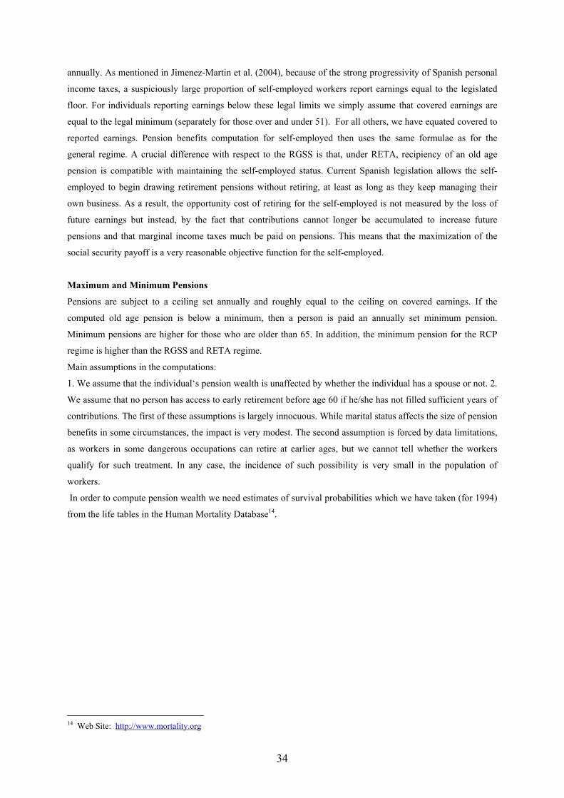
34

annually. As mentioned in Jimenez-Martin et al. (2004), because of the strong progressivity of Spanish personal

income taxes, a suspiciously large proportion of self-employed workers report earnings equal to the legislated

floor. For individuals reporting earnings below these legal limits we simply assume that covered earnings are

equal to the legal minimum (separately for those over and under 51). For all others, we have equated covered to

reported earnings. Pension benefits computation for self-employed then uses the same formulae as for the

general regime. A crucial difference with respect to the RGSS is that, under RETA, recipiency of an old age

pension is compatible with maintaining the self-employed status. Current Spanish legislation allows the self-

employed to begin drawing retirement pensions without retiring, at least as long as they keep managing their

own business. As a result, the opportunity cost of retiring for the self-employed is not measured by the loss of

future earnings but instead, by the fact that contributions cannot longer be accumulated to increase future

pensions and that marginal income taxes much be paid on pensions. This means that the maximization of the

social security payoff is a very reasonable objective function for the self-employed.

Maximum and Minimum Pensions

Pensions are subject to a ceiling set annually and roughly equal to the ceiling on covered earnings. If the

computed old age pension is below a minimum, then a person is paid an annually set minimum pension.

Minimum pensions are higher for those who are older than 65. In addition, the minimum pension for the RCP

regime is higher than the RGSS and RETA regime.

Main assumptions in the computations:

1. We assume that the individual‘s pension wealth is unaffected by whether the individual has a spouse or not. 2.

We assume that no person has access to early retirement before age 60 if he/she has not filled sufficient years of

contributions. The first of these assumptions is largely innocuous. While marital status affects the size of pension

benefits in some circumstances, the impact is very modest. The second assumption is forced by data limitations,

as workers in some dangerous occupations can retire at earlier ages, but we cannot tell whether the workers

qualify for such treatment. In any case, the incidence of such possibility is very small in the population of

workers.

In order to compute pension wealth we need estimates of survival probabilities which we have taken (for 1994)

from the life tables in the Human Mortality Database14.

14 Web Site: http://www.mortality.org

35

APPENDIX 2: Additional tables

Descriptives of pension wealth, accrual and peak value

Table A1 shows the median of pension wealth, accrual and peak value incentives, as well as the first and ninth

decile of accrual and peak values in our sample.

The median PW starts off at 138,185 Euros and peaks between 64 and 65 years of age at 159,009 Euros.

Remember that PW reaches its maximum value just at the age which the worker is allowed to retire (normal

retirement age). The median of pension wealth from age 57 to 60 decreases. Median of PW rises again after the

age of 60 until 65. A negative accrual can be interpreted as a tax on further labor force participation. The 10th

percentile of the accrual value is positive until age 60and turns negative above 60. Again this is consistent with

the fact that pension wealth cannot decrease by postponing retirement one year for ages under 60. The median

accrual is positive until age 65 and becomes negative after age 65: the increase in the pension for each additional

year is too weak to compensate the loss of one year of pension. The accrual after age 60 is negative in 10% of

the distribution. For those individuals, the implicit tax rate on continuing work can be higher; is these

individuals are also on low income, the effect on incentives for early retirement may be strong.

The median peak value and accrual value show similar profiles. However, from age 55 to 64, the median peak

value is much higher, reinforcing retention incentives in that age range.

Table A1: Pension Wealth, Accrual and Peak Value Incentive Measures for all regimes (in 2001 Euros)

Accrual

Value

Peak

Value

Age Obs Median PW P10 P50 P90 P10 P50 P90

55 551 138,185 3,667 7,446 17,323 12,934 62,885 161,880

56 578 139,800 3,593 7,906 18,374 17,784 61,763 153,644

57 625 132,891 3,505 7,172 16,628 15,282 57,679 144,002

58 591 130,839 3,411 6,914 15,847 14,581 53,135 137,008

59 550 126,569 3,276 6,684 16,544 12,102 51,420 128,990

60 512 120,014 -694 13,937 32,536 2,629 56,013 123,953

61 496 129,367 -1,373 12,258 30,770 897 41,390 101,909

62 437 137,101 411 11,581 33,015 895 32,058 81,165

63 397 150,824 -1,055 9,906 24,781 390 19,551 60,289

64 388 155,373 -1,294 7,853 22,390 -809 9,152 35,843

65 301 159,009 -6,410 -1,420 6,142 -6,217 -831 14,106

66 227 150,181 -8,032 -1,395 4,760 -8,032 -1,206 10,100

67 159 146,647 -7,058 -2,157 1,994 -7,058 -2,157 2,957

68 118 140,280 -5,658 -2,814 502 -5,658 -2,814 502

69 75 122,982 -6,195 -2,566 455 -6,195 -2,566 455