Does Contract Enforcement Limit the Distribution of Bargaining Power? AnExperimental Study

Selected Paper No. 302

Paula Cordero SalasEconomics, Finance and Legal Studies, University of Alabama.

Contact information: Tel.:+1 205-348-5633; 361 Stadium Drive, 250 Alston Hall,Tuscaloosa, AL 35487-0224.

Email address: pcordero@cba.ua.edu.

Selected Paper prepared for presentation at the Agricultural & AppliedEconomics Association’s 2012 AAEA Annual Meeting, Seattle, Washington,August 12-14, 2012

Copyright 2012 by Paula Cordero Salas. All rights reserved. Readers may make verba-tim copies of this document for non-commercial purposes by any means, provided thiscopyright notice appears on all such copies.

1

Does Contract Enforcement Limit the Distribution of Bargaining

Power? An Experimental Study ∗†(Preliminary: do not cite without permission.)

Comments welcome

Paula Cordero Salas‡

May 31, 2012

Abstract

In more consolidated markets where asymmetric bargaining power leaves one party with smallcontract rents, policies that attempt to balance bargaining power may be implemented. The eco-nomic effects of such policies depend on the degree of legal enforcement. This paper examineshow redistributing bargaining power among sellers and buyers affects long-term relationships whenthird party enforcement is partially and fully absent. I implement an experimental design thatadjusts the bargaining power of sellers and the enforceability of the contract. I find that bargainingincreases the use of efficiency wage contracts when partial enforcement is available. When enforce-ment is absent, bargaining has a negative effect on cooperation if it is actually exercised but it doesnot deter trade and does not affect the overall level of efficiency. However, contract enforcementlimits the exercise of bargaining power. Sellers get higher rents if bargaining is implemented whencontracts are partially enforceable. Regardless of the distribution of bargaining power sellers get ahigher share of the surplus when partial enforcement is in place. These results provide insight foreconomic policy into the consequences of shifting bargaining power in market settings characterizedby informal institutions.

Key words: contracts, incomplete enforcement, bargaining, experiments, distribution, institutions.JEL Codes: D86, K12, L14, O12, Q13.

∗I thank Brian Roe, Steven Wu, Jack Schieffer, John Kagel, Tim Cason, Paul Healy, Kevin Pflum and theExperimental Economics Work group at Purdue University for very useful comments and discussion.†Acknowledgments: This project was supported by the National Research Initiative of the Cooperative State

Research, Education and Extension Service, USDA, Grants #2008 − 35400 − 18701 and #2005 − 35400 − 15963 andthe Farm Income Enhancement Program at Ohio State University, and also by the OSU Graduate Schools AlumniGrants for Graduate Research and Scholarship.‡University of Alabama Tel.:+1 205-348-5633. Email address: pcordero@cba.ua.edu. Postal address: 361 Stadium

Drive, 250 Alston Hall, Tuscaloosa, AL 35487-0224.

2

1 Introduction

The ability of parties to enforce agreements is key for efficient performance and economic develop-

ment. In developing countries, where legal enforcement is weak, parties often use informal incentives

and good faith to self-enforce agreements. However, the existence of asymmetric bargaining power

among parties that operate in more consolidated markets has risen concerns about the distribution

of the contract rents, especially when formal contract enforcement is incomplete (Lee, 2002; Mac-

Donald et al., 2004; the Democratic Staff, 2004). This is particularly true in the agricultural sector,

in which verification of product attributes may be very costly and some dimensions of performance

such as timing of delivery or contract renewal policies are not explicitly included in contracts. Some

agricultural contracts often specify a payment formula which includes a base price and adjustments

from it in the form of premiums and discounts which depend on the observed product character-

istics. This contract structure endows buyers with a higher discretionary power to adjust final

payments and leave farmers with lower contract rents. Even in developed countries, farmers have

complained about the unfairness in agricultural contracts (Lee et al., 2008; Love and Burton, 1999;

MacDonald et al., 2004; Wu, 2006).

In this context, policies that attempt to balance bargaining power have been discussed and

sometimes implemented with little knowledge about their consequences on self-enforcing contracts.1

Past literature have looked bargaining and relational contracts in separate settings. In fact, litera-

ture regarding the effect of bargainining on relational contracting is scarse. This paper fills this gap

by examining new experimental evidence on how redistributing bargaining power among sellers and

buyers affects long-term relationship, efficiency and surplus distribution when third party enforce-

ment is partially and fully absent. I find that bargaining does not improve overall social efficiency

or increase the sellers’ contract rents as bargaining introduces a new source of inefficiency. Fur-

themore, the implementation of only partial enforcement results in a pareto improvement outcome

relative to the implementation of bargaining with partial or fully incomplete enforcement: overall

social surplus is higher and sellers and buyers share the surplus more equally. These results provide

1For example the Agricultural Fair Practices Act in 1967, the Producer Protection Act in 2000 and the 2010 PatientProtection and Affordable Care Act (PPACA) in the U.S. and the Australian Trade Practices Act in Australia.

3

insight into the economic consequences of shifting bargaining power in relational contracting and

provide some guidance to draw policies that attempt to improve bargaining conditions of weaker

parties when they trade in market settings characterized by informal institutions.

I implement an novel experimental design that adjusts the bargaining power of sellers (agents)

and the enforceability of the contract. In the main treatments, sellers may counteroffer after

rejecting a buyers’ first offer while contract enforcement is partially or fully absent. In the control

treatments, sellers only accept or reject buyers’ first offers. If parties agree on a contract, they

trade one unit of a good which quality is not contractible, and parties have the latitute to decide

if they comply with the quality and compensation in the contract or if they deviate by choosing

lower quality provision and payments.

I find that the possibility of bargaining has positive impact in the overall rate of cooperation

and does not deter trade when formal enforcement is absent; however, when sellers actually exercise

their bargaining power cooperation decreases because buyers behave opportunistically as their

payoffs shrink. Enforcement does not change the level of cooperation but it improves social surplus

by increasing the number of trades relative to when bargaining is not in place (decreases efficiency

loss due to loss trade). Bargaining increases the level of quality traded when enforcement is fully

absent, but the gains of trade from such higher quality are eroded by the use of bargaining power

(increases efficiency loss due to bargaining). When contract enforcement is partial, bargaining does

not affect the level of quality traded or the number of trades, but the exercise of bargaining power

taxes the social surplus generated resulting in a lowering surplus to distribute.

Contract enforcement limits the exercise of sellers’ bargaining power. Sellers reject more of

the buyers’ offers and use counteroffers more in the presence of partial contract enforcement than

when contract enforcement was fully absent. The evidence shows that enforcement supports sellers’

exercise of bargaining power. In fact, bargaining did not increase the overall sellers’ payoffs or share

of overall surplus regardless of the enforcement level. Bargaining was only effective in increasing

sellers’ share of surplus and payoffs for completed transactions and when partial enforcement was

in place. In contrast, enforcement has a positive and significant effect on overall sellers’ rents.

When partial enforcement is in place, bargaining affects contract structure by increasing the

4

size of the price and lowering the size of the bonus included in the contract. As consequence con-

tracts take the form of efficiency wage contracts when bargaining and enforcement are implemented.

From a policy perspective, if the goal is to increase the contract rents for the weaker party

through an improvement of her bargaining position, the evidence in this paper suggests that a policy

to shift bargaining power needs to be coupled with the implementation of formal enforcement of at

least of an up-front payment. However, the social planner can minimize the efficiency loss due to

bargaining and still achieve a more egalitarian distribution of the surplus if only formal enforcement

is implemented.

Related Literature. This paper related to existing literature on relational contracts and bar-

gaining. On one hand, literature has looked at market interactions and the existence of relational

contracts under different enforcement conditions. Brown et al. (2004) (hereto referred to as BFF)

use experimental economics to show how the absence of third-party enforceability impacts the

nature of market interactions including the initiation of contracts, formation of long-term relation-

ships, contract terms and how all these affect efficiency and the distribution of the surplus generated

by trading. The experiment simulates firm-worker relationships and they implement three different

treatments to test the endogenous emergence of long-term relationships.

Wu and Roe (2007b) (hereto referred to as WRb) also use experimental economics to examine

how the nature and efficiency of trade differs across different relational contracting environments.

WRb’s model is based on a buyer-seller relationship and use the same design and implement

two treatments from BFF. Additionally, they implement two incomplete contracting treatments

in which buyers can adjust prices ex post. Both of these papers examine cooperation and long-

term relationships under different contract enforcement regimes. However, they maintain constant

bargaining power across treatments. In essence firms (buyers) make take-it-or-leave-it offers that

workers (sellers) accept or reject (ultimatum game). In contrast, the experimental design of this

paper varies the bargaining power exogenously across treatments. In the main treatments subjects

play a bargaining game to agree on contract terms. In addition, treatments with an ultimatum

game are also implemented and are used as control treatments. Furthermore, the experiment here

differs from previous contracting experiments in the implementation of an infinite repeated game

5

while only finite repeated games have been previously implemented.

On the other hand, bargaining has been examine in laboratory setting by using a variety

of games including ultimatum and alternating offer games. Examples of this literature are Ochs

and Roth (1989) Guth et al. (1982), Prasnikar and Roth (1992), Roth and Murnighan (1982) and

Kagel et al. (1996). This experimental evidence indicates that in games where participants have

symmetric payoffs and full information the first mover obtains a medium return of the 60% of the

total surplus or less. However, it is not clear how subjects respond in a more complex environment

in which they have to split the surplus generated through a gift exchange game.

In contrast to this research, the papers cited do not implement the bargaining game in a

contracting context in which there is enforcement variability. In fact, literature regarding the effect

of shifting bargaining power on relational contracting under diverse enforcement regimes is scarce.

This paper contributes to the literature by testing the hypothesis derived from a theoretical model

( Cordero Salas (2011)) where bargaining power is shifted in the context of self-enforcing, relational

contract theory and by implementing a new experimental design in which an alternating offer game

is jointly implemented with a gift exchange game.

The structure of the paper is as follows. Section two develops briefly the model. Section

three describes the experimental design and procedures. Section four forward the predictions and

hypothesis. Section five presents the results and section six concludes.

2 Relational Contracting Model with Bargaining

I briefly outline the relational contracting model with bargaining (Cordero Salas (2011)). Assume

a buyer and a seller have the opportunity to trade one unit of a good of quality qt ∈ Q = [q, q] at

dates t = 0, 1, 2, 3 . . .. Quality is observable by both parties but it is not enforceable by a neutral

third party. Payments may or may not be enforceable depending on the enforcement regime. At

the beginning of each period t, the buyer and the seller are aware of the enforcement regime and

engage in a Nash bargaining process over the profit-sharing rule included in the contract. A contract

includes a total compensation defined as Pt(qt) = pt + Dt(qt) and consists of a base payment, pt,

and a contingent-payment, Dt(qt). The base payment is not enforceable when contract enforcement

6

is fully incomplete but it is enforceable if partial enforcement is implemented. In contrast, the

contingent payment always depends on unverifiable quality, therefore it is never contractible. A

negative Dt = d(qt) is a discount and is used as a punishment or for deviations from the buyer

when pt is not contractible. A positive Dt = b(qt) is a bonus and is used to reward high quality. 2

If parties agree on a contract in the bargaining phase, they move into the trading phase and

make independent decisions about quality and payments. The seller chooses the quality qt ∈ Q

to deliver and incurs a cost ct(qt), where c′(.) > 0, c′′(.) ≥ 0, and c(q) = 0. The seller’s profit

per trading round is Ut = Pt(qt) − ct(qt). The seller’s quality provision generates a direct benefit

for the buyer, Rt(qt), where R′(.) > 0, R′′(.) ≤ 0, and R(q) = 0. The buyer chooses whether to

pay bt(qt) and, in the fully incomplete enforcement regime, pt. The buyer’s profit for the trading

round is given by πt = Rt(qt) − Pt(qt). It is also assumed that R′(.) > c′(.) ∀ q ∈ Q, so that it is

socially efficient and Pareto optimal to trade q = q, since q maximizes the total surplus defined by

S(qt) = R(qt)− c(qt). This sequence of events repeats in each period t (figure ?? illustrates a single

stage of the repeated game).

If disagreement occurs while parties bargain, they receive zero payoffs. If either party decides

to opt out of the bargaining process trade does not occur, the game ends and both parties receive

fixed payoffs: u for the seller and π for the buyer. These fixed payoffs are assumed to be less

attractive than trading, and any breakdown in trade represents a socially inefficient outcome.

Assume that s = u + π and the net social surplus is S(qt) − s, where S(qt) − s > 0 ∀ q ∈ (q, q],

and S(q) > S(q) ≥ 0. Parties bargain over the surplus and each party’s share through the contract

needs to satisfy the individual rational constraint (IRC) for the seller, U = P (q)− c(q) ≥ u and for

the buyer, π = R(q)− P (q) ≥ π.

As parties bargain over the contract terms, the optimal contract reflects how the surplus is

split depending on the bargaining power that each party exercises in the bargaining process. The

bargaining outcomes are derived from an application of the asymmetric Nash bargaining solution

2Most papers in relational contracts—e.g. Levin (2003)—assume that the decision to use the contingent paymentbelongs to the buyer if the adjustment is positive (bonus) and to the seller if it is negative (deduction). In this model,the decision belongs only to the buyer, as this case mimics supply agricultural contracts where all payments are madeex post depending on quality delivered. Furthermore, Iskow and Sexton (1992) find that fruit and vegetable growersoften complain about payments made well after delivery, which supports the assumption about the base payment inthe fully incomplete case in this paper.

7

(ANBS) with outside options where β represents the bargaining power of the seller. As a result,

the optimal contract, satisfies Ut(y∗i ) = βS(q) and πt(y

∗i ) = (1 − β)S(q) where βS(q) ≥ u and

(1− β)S(q) ≥ π respectively such that the IRCs are satisfied.

Parties interact repeatedly and care about the stream of payments where the common dis-

count factor is δ ∈ (0, 1]; parties support future trade contingent on the satisfactory performance of

present trade. The parties cooperate if the history of play in all periods has been cooperation, and

break-off trade forever if any deviation is observed (as assumed in Levin (2003)). Additionally, each

period is played following a Nash equilibrium, parties use stationary contracts and repetition allows

players to self-enforce the contract and maintain a Subgame Perfect Nash Equilibrium (SPNE).

When contracts are fully unenforceable, neither the quality nor the base price pt or the

bonus are enforceable. Since parties can deviate from the contract without a formal penalty, the

optimal contract must additionally satisfy a dynamic incentive compatibility constraint (DICC) for

each party such that it insures the parties get more gains from honoring the contract than from

reneging. The contract also has to satisfy both IRCs and bargaining outcomes. The DICC are

given by p+b(q)−c(q)1−δ ≥ p+d(qt)− c(q) + δ

1−δu for the seller and R(q)−p−b(q)1−δ ≥ R(q)−p−d(q) + δ

1−δπ

for the buyer, where the left hand side are the gains from cooperation and the right hand side

represents the gains from deviation respectively. Note that the most profitable deviation for the

seller is to supply q, but in this case the buyer after observing quality delivered, sets the total

payment to zero by imposing dt(qt) = −pt. By the same token, the most profitable deviation for

the buyer is to pay nothing.

Given the IRCs, the bargaining outcomes and the DICCs when contract enforcement is fully

incomplete, an optimal stationary with a total compensation of P (q) = c(q) + βS(q), implements

the optimal level of quality, q, if the parties have a discount factor

δ > δ̂IE ≡c(q) + βS(q)

R(q)− π.

This implies that self-enforcing constraints the effective bargaining power the seller can ex-

ercise. In equilibrium, the seller can only exercise a bargaining power β < β̂ ≡ δR(q)−δπ−c(q)S(q)

and continue the relationship. Then, the compensation scheme is characterized by: b(q) − d(q) ≥

8

c(q) − δ1−δ (βS(q) − u) and p = −d(q) + βS(q)−δu

1−δ . In this case, there is little to say about the

structure of the incentive provision since the base price is indeterminate because it also contains

the value of the discount. Intuitively, this reflects the enforcement incompleteness as the base price

is inversely related to the buyer’s latitude to adjust the total payment to zero and that the total

payment is all contingent on performance.

Proposition 1. Cooperation and full efficiency depend on the exercise of the seller’s bargaining

power. Cooperation and full efficiency is the equilibrium outcome if βS(q) = u and δ > δ̂IE ≡c(q)+uR(q)−π , or if β ≤ β̂. If β > β̂ trade breaks down causing an efficiency loss.

Proposition 2. Self-enforcing constraints the effective bargaining power the seller can exercise and

the rents she can get.

If partial enforcement is implemented, the total payment includes pt, which is now con-

tractible, and bt(qt) that the buyer promises to pay as long as the seller does not shirk. The

optimal contract also needs to satisfy the parties’ DICC. In this case, the seller cooperates if only

if p+b(q)−c(q)1−δ ≥ p− c(q)+ δ

1−δu. Note that the most profitable deviation for the seller is to supply q,

but in this case the buyer after observing the quality, will not pay the bonus. On the other hand,

a buyer cooperates if and only if R(q)−p−b(q)1−δ ≥ R(q)− p+ δ

1−δπ. The most profitable deviation for

the buyer is to withhold the bonus.

Given the IRCs, the bargaining outcomes and the DICCs, when contracts are partially en-

forceable, an optimal stationary contract with a total payment of P (q) = c(q) +βS(q), implements

the optimal level of quality, q, if the parties have a discount factor

δ > δ̂PE ≡c(q)

R(q)− u− π,

and the compensation scheme is characterized by: b(q) = c(q)− δ1−δ (βS(q)− u) and p = βS(q)−δu

1−δ .

Note that as the seller’s bargaining power increases, the contract takes the form of efficiency wages

and not contingent performance payments to induce the seller’s performance.

Proposition 3. If the base payment is enforced and δ > δ̂PE ≡ c(q)R(q)−u−π , cooperation and full

efficiency is the equilibrium outcome regardless of the distribution of bargaining power.

9

Proposition 4. The seller can exercise full bargaining power and receive rents accordingly. The

efficient self-enforcing contract takes the form of a bonus contract when the seller’s bargaining power

is low and takes the form of an efficiency wage contract when the seller’s bargaining power is high.

3 Experimental Design

I implement a variation of the repeated labor market experimental design of Brown et al. (2004) and

the repeated supply market experiments of Wu and Roe (2007a,b). I modify the basic experimental

platform to test the model predictions and examine how bargaining power affects the formation

of long-term relationships and market outcomes. The supergame consists of an infinite market

interaction between sellers and buyers in contrast to the finite games implemented by Brown et

al. (2004) and Wu and Roe (2007a,b). Buyers and sellers use contracts to establish the terms of

trade for one unit of a good. In the first treatment, which I call no contract enforcement with

no bargaining (NN), I implement an ultimatum game in which the buyer makes take-it-or-leave it

offers to the seller and the seller, upon acceptance, may choose any feasible quality irrespective of

the contractually agreed upon level. The buyer could also choose any feasible level of price and

bonus, therefore the buyer has the latitude to adjust the total payment to zero. That is, the total

payment is discretionary and contingent on quality delivered. In the second treatment, which I

call no contract enforcement with bargaining (NB), I allow sellers to counteroffer the buyer one

time after he has made the first offer (implements an alternating offer game with two offers). The

buyer could also adjust the total payment to zero. In the third and fourth treatments, which I

call the partial contract enforcement condition with no bargaining (PN) and the partial contract

enforcement condition with bargaining (PB), I implement the ultimatum game and the alternating

offer game as in the NN and NB conditions respectively, but in these two treatments the price is

exogenously enforced by the computer while all other variables in the contract are not enforced.

Then, the buyer could also choose any feasible (non-negative) level of bonus. Figure 1 summarizes

the treatments.

In each treatment, subjects were exogenously matched into pairs of one buyer and one seller

that interacted anonymously through the computer network. A random termination rule was

10

Treatments  

Contracting with no enforcement and no

bargaining (NN)

Contracting with no enforcement and with

bargaining (NB)

Contracting with partial enforcement and no

bargaining (PN)

Contracting with partial enforcement and bargaining (PB)

Parameters Feasible quality Feasible price and bonus

v=10, c=5

v=10, c=5

v=10, c=5 v=10, c=5

Contract terms determination

Buyers make take-it-or leave-it offers

Sellers can counteroffer; alternating offer game with

two offers.

Buyers make take-it-or leave-it offers

Sellers can counteroffer; alternating offer game with

two offers.

Exogenously enforced contract terms

None None Price Price

Termination rule implemented

Predictions: rational money maximizes

Self-enforcement sustainable in every period ( needed for cooperation) Profit buyer=45 Profit seller=5

Self-enforcement sustainable in every period if sellers exercise low bargaining power ( ) Profit buyer=20 Profit seller=30

Self-enforcement sustainable in every period ( needed for cooperation) Profit buyer=45 Profit seller=5

Self-enforcement sustainable in every period ( needed for cooperation) Profit buyer=5 Profit seller=45

q ! (1,10)p,b! (0,100)

q ! (1,10) q ! (1,10) q ! (1,10)p,b! (0,100) p,b! (0,100)p,b! (0,100)

! = 4 5

! =1120

P = 55;q =10.

! = 4 5! = 4 5! = 4 5

P = 80;q =10.! = 0.6

! =1019

p =10;b = 45;q =10.

! =1019

p = 95;b = 0;q =10.

Figure 1: Summary of treatment conditions

implemented such that subject pairs played for an infinite number of periods. Subjects knew that

they would keep trading with the same partner for an additional period with a 4/5 probability. This

commonly known probability of continuation controlled for subjects’ belief about the possibility of

future interaction. Then, each pair expected to play together for 5 periods.3

The stage game in all treatments has two sub phases: a negotiation phase and a trading

phase. Figure 2 summarizes the sequence of action in the stage game. In the negotiation phase

of the treatments with no bargaining, each buyer makes a take-it-or-leave-it- contract offer to

his matched seller. The seller decides to accept or reject the contract. If the seller accepts, the

pair moves to the trading phase. If the seller rejects, the pair does not trade in that period. In

contrast, in the treatments with bargaining, if the seller rejects the offer, she can offer a contract

(counteroffer) to the matched buyer. In this case, the buyer gets to accept or reject. If the buyer

accepts, the pair moves to the trading phase where the traded good gives lower benefits to the

parties if they have traded through counteroffers. If the buyer rejects, the pair does not trade in

that period. Each proposed contract included a level of quality, a price and a bonus. The set of

allowable qualities is {1, 2, . . . , 10} and the set of allowable prices and bonus is {0, 1, 2, 3, . . . , 100}.

The trading phase consists in two phases: quality determination and payment determination.

Because quality is discretionary in all treatments, the quality determination sub phase was the same

for all treatments and sellers could choose any quality from 1 to 10. The payment determination

sub phase differs from the partial enforcement (PE) to the no enforcement (NE) treatments. In

the PE treatments, the price is binding and the computer ensures that the price specified in the

3The expected number of periods of a game with a continuation probability of δ is equal to T = 11−δ

. Therefore,with δ = 4/5 the expected number of periods each pair interacts equals 5.

11

contract is paid, which ranges between 0 and 100. In the NE treatments the computer does not

enforce the price such that the buyer can chose to pay a different price than the one in the contract;

in both treatments buyers can choose any bonus ranging from 0 to 100 after observing the quality.

Therefore, a buyer in the NE treatments can adjust the total payment to zero while in the PE

treatments a buyer has to pay the contracted price. Once all decisions are made, payments are

made and each party receives payoffs.

Terms of the contract

including : (p, b(q), q)

Payments

are madeIn all

treatments,

seller chooses Q

that may differ

from contract

If PE computer

enforces fixed

payment and buyer

may choose a

different

performance

payment

If NE buyer

may adjust

payment to

zero

If PN or NN

buyers make

take-it-or-leave-

it offers.

Phase 1: Negotiation Phase 2: Trading

Sub phase 1: Quality Determination Sub phase 2 : Price Determination

If PB or NB

buyers make

offers and

seller may

counteroffers

If contract

go to next

phase

Figure 2: Stage game by phases for all treatments

The stage game payoffs in the no bargaining treatments (PN and NN) for the buyer, πNBB ,

and seller, πNBS , are given by

πNBB =

10Q− p− b(Q) if contract was concluded

0 if contract was not concluded

πNBS =

p+ b(Q)− 5Q if contract was concluded

5 if contract was not concluded

In the bargaining treatments (PB and NB), the discount factor in the alternating offer game

with two offers is included in the payoff functions, β = 0.9. It reflects the cost of delay trade for the

player who makes a counteroffer (seller). If a buyer accepts a counteroffer, he receive discounted

profits by 0.1. The payoffs are given by :

12

πBB =

10Q− p− b(Q) if contract was concluded with a first offer

(0.1)(10Q− p− b(Q)) if contract was concluded under a counteroffer

0 if contract was not concluded

πBS =

p+ b(Q)− 5Q if contract was concluded with a first offer

0.9(p+ b(Q)− 5Q) if contract was concluded under a counteroffer

5 if contract was not concluded

The cost for all sellers was 5Q. If subjects did not trade, the seller got 5 points and the

buyer 0. All buyers and sellers in the same treatments face the same payoff parameters in all

experimental sessions. Payoff functions, the cost schedule and the termination rule were common

knowledge. However, only the pair of traders involved in each transaction were informed about the

actual payoffs and quality level delivered. Therefore, parties could only build a reputation with the

partner with whom they were trading.

At the end of each trading period, each participant is informed about the contract (p, b(q), q)

he had concluded, the actual quality delivered, q, the payment made, his own payment, as well as

about his trading partner’s payoff.

3.1 Procedures

Session were run at the Experimental Economics Laboratory at the Ohio State University using

undergraduate student from a variety of majors recruited via E-mail. Table 1 summarizes informa-

tion about the 17 experimental sessions that have been held. At check in subjects were assigned

a random ID number to preserve anonymity. Each subject was randomly assigned to a networked

computer and was told that they will participate in a computerized trading experiment. The ex-

periments were programmed using the Z-TREE software (Fischbacher, 1999) and took place on

networked computers. At the beginning of the experiment participants were randomly assigned to

13

the role of either a buyer or a seller. These roles were fixed for the duration of the session. Each

subject had an identification number for the role (IDR), e.g. buyer 1, seller 5 which was also fixed

during each contracting game allowing subjects to keep track of trading partners. Each buyer was

paired randomly with a seller. Each pair played an uncertain number of trading games. There were

R = T ∗N/2 trades per game, where N is the number of subjects participating in the session and

T is the number of periods played in each game.

One single treatment was run in each experimental session and a different group of subjects

participated in each session. Each experiment consisted of a trial unpaid game, two surveys, a

control questionnaire and the paid treatment. The treatment was run one to six times, where

the number of times depended on the results of the random termination rule and the time left

after each termination. Each time subjects were matched with a different partner and they played

together until the continuation rule indicated. All sessions lasted between one and half and two

hours depending on the random termination rule.

Instructions for the main treatment were read aloud for both buyers and sellers and each

subject was given a printed copy for reference. When instructions were read, subjects did not

know whether they had been assigned to be buyers or sellers. In addition, subjects answered a

computerized control questionnaire formulated to test understanding of the treatment. In order

to help the subjects to understand the game structure, the questionnaire contained hypothetical

situations in the game from the perspective of both roles, buyers and sellers, and the correct answers

were provided afterwards. The trading game did not start until all subjects understood the game.

To further ensure that all subjects understood the game, after completing the control questionnaire,

subjects were assigned randomly to be sellers or buyers, and participated in two practice rounds.

The practice rounds were identical to normal rounds with the exception that no money was earned.

Practice rounds had the purpose of familiarizing subjects with the computer controls and screens.

Subjects were not able to see actual choices or payments in order to avoid possible deception.

Once the practice periods were over, the real periods of the game started. Each subject

received a $5 balance in their account (250 experimental points). Because of the random termination

rule, some experiments were longer than others and if the experiment ended prior to the allotted

14

time for the evening’s session, then additional games were played until the allotted time expired.

For each new game, subjects were matched with a different partner, avoiding any possibility of

contagion effects across treatments.

Once all games were over, subjects were asked to complete an exit survey while experimenters

determined payouts. Finally, subjects were paid privately. The subjects earned a show-up fee

plus additional earnings that were proportional to the points earned during the experiment. The

exchange rate was 50 experimental points per $1 which ensured that subjects had incentives to

increase their points earnings. Subjects earned an average of $16.61 with a maximum $32 and a

minimum of $6.

4 Predictions and Hypothesis

The socially efficient level of quality is Q = 10 because marginal revenue (10) is greater than

marginal cost (5) for all quality levels. The efficient level of quality maximizes the social surplus

at 50. Participants are assumed to be self-interested, risk-neutral utility maximizers and that this

is common knowledge. The degree of cooperation in each treatment is defined as the proportion of

subject pairs that honor the the contract, the seller supplying the contracted quality and the buyer

paying the contracted payment. The acceptance rate reflects the willingness to trade. I denote q

as the requested quality and q∗ as the delivered quality.

4.1 Treatment 1: No enforcement, no bargaining (NN)

When contract enforcement is absent and no bargaining takes place, the ongoing interaction sustains

the efficient outcome for discount factors equal to or greater than δNE = c(q)+uR(q)−π = 5Q+5

10Q = 0.55.

Then, cooperation is sustainable and efficiency is reached in every period for the probability of

continuation used in the experiments, δ = 4/5. The predictions are summarized as follows.

Prediction 1. The buyer offers a contract (P (q), q) = (55, 10) and the seller accepts.

Prediction 2. In each period, the efficient outcome is sustained, actual quality equals 10 and

surplus equals 50. The equilibrium payoffs are (πB, πS) = (45, 5) for the buyer.

15

Prediction 3. Cooperation is observed in every period.

This treatment is conductive to cooperation under the assumptions of the model because for

any quality greater than one, the gains from cooperation are greater than the gains from deviation

for both parties. For any given quality level, the ICCs reduce to p + b(q) ≥ 5Q + 4 for the seller,

and 10Q ≥ p + b(q) for the buyer. For example, if parties trade at a quality level of 2, the buyer

pays P (q) = 15 (as the seller’s IRC binds) and the payoffs are (πB, πS) = (5, 5), which satisfies

incentive compatibility. The minimum discount factor that would sustain cooperation when the

traded quality is 2, is 3/5, which is lower than the termination rule used. Then, even for low quality

levels, cooperation is the dominant strategy.

4.2 Treatment 2: No enforcement, with bargaining (NB)

The second treatment, NB, is identical to the NN treatment with the exception that sellers can ex-

ercise bargaining power by using counteroffers. In this treatment, cooperation sustains the efficient

outcome if δNE ≥ c(q)+βS(q)R(q)−π = 5Q+0.5∗5Q

10Q = 0.95. The continuation probability of δ = 4/5 used does

not sustain cooperation if the sellers exercise all their bargaining power, in which case, the buyer’s

dynamic incentive compatibility constraint is not satisfied 10Q−9.5Q0.2 ≥ 10Q + 0 ⇒ 0.5Q ≥ 2Q.

Then, for any given quality, the buyer gets a higher payoff by deviating.

Self-enforcement limits the sellers’ exercise of bargaining power in this treatment, but if sellers

exercises less bargaining power, the efficient outcome can be sustained by increasing the buyers’

stage payoff from cooperating. That is the seller claims less of the surplus by accepting a lower

payment. The buyer’s self-enforcing constraint sets the maximum bargaining power the seller can

exercise without the buyer reneging, 10Q−5Q−β5Q0.2 ≥ 10Q ⇒ 3/5 ≤ β. If the seller only exercises a

bargaining power equivalent to 0.6 cooperation is sustained and the efficient outcome is achievable.

Prediction 4. If the sellers exercise all available bargaining power the efficient outcome is not

sustained. The buyers take short term profits and deviation is observed in every period.

Prediction 5. If sellers exercise bargaining power of 0.6 or less, the efficient outcome is sustain-

able, actual quality equals 10 and the surplus equals 50. The seller accepts the equilibrium contract

(P (q), q) = (80, 10) and the equilibrium payoffs are (πB, πS) = (20, 30).

16

Prediction 6. Cooperation is observed in every period if sellers exercise β ≤ 0.6.

This treatment is less conductive to cooperation, when compared to the NN treatment.

Subjects in the role of sellers can use counteroffers to increase their payoffs and claim most of

the surplus. Moving from payoffs (πB, πS) = (2Q, 3Q) to any distribution that gives less profit to

the buyer and more to the seller, triggers deviation from the buyers. Then, the set of contracts for

which cooperation is the dominant strategy is smaller. Furthermore, the possibility of counteroffer

introduces an additional source of inefficiency because bargaining is costly and the surplus available

for the parties shrinks. Consequently, this treatment is less conductive to efficiency but sellers

ambiguously get higher payoffs.

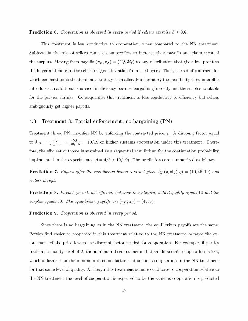
4.3 Treatment 3: Partial enforcement, no bargaining (PN)

Treatment three, PN, modifies NN by enforcing the contracted price, p. A discount factor equal

to δPE = c(q)R(q)−u = 5Q

10Q−5 = 10/19 or higher sustains cooperation under this treatment. There-

fore, the efficient outcome is sustained as a sequential equilibrium for the continuation probability

implemented in the experiments, (δ = 4/5 > 10/19). The predictions are summarized as follows.

Prediction 7. Buyers offer the equilibrium bonus contract given by (p, b(q), q) = (10, 45, 10) and

sellers accept.

Prediction 8. In each period, the efficient outcome is sustained, actual quality equals 10 and the

surplus equals 50. The equilibrium payoffs are (πB, πS) = (45, 5).

Prediction 9. Cooperation is observed in every period.

Since there is no bargaining as in the NN treatment, the equilibrium payoffs are the same.

Parties find easier to cooperate in this treatment relative to the NN treatment because the en-

forcement of the price lowers the discount factor needed for cooperation. For example, if parties

trade at a quality level of 2, the minimum discount factor that would sustain cooperation is 2/3,

which is lower than the minimum discount factor that sustains cooperation in the NN treatment

for that same level of quality. Although this treatment is more conducive to cooperation relative to

the NN treatment the level of cooperation is expected to be the same as cooperation is predicted

17

be observed in every period given the parameters used in the experiment. Because no bargaining

takes place and partial enforcement is available, high efficiency is more likely than in the NN and

NB treatments.

4.4 Treatment 4: Partial enforcement, with bargaining (PB)

The fourth treatment, PB, alters NN by enforcing the contracted price, p, and allowing sellers

to make counteroffers. Cooperation is also sustainable for discount factors greater than or equal

to δPE = c(q)R(q)−u = 10/19. Therefore, the efficient outcome is sustained given the continuation

probability of 4/5 implemented. The predictions are summarized as follow.

Prediction 10. Buyers offer the equilibrium efficiency wage contract (p, b(q), q) = (95, 0, 10) and

sellers accept.

Prediction 11. In each period, the efficient outcome is sustained, actual quality equals 10 and the

surplus equals 50. The equilibrium payoffs are (πB, πS) = (5, 45).

Prediction 12. Cooperation is observed in every period.

Although the discount factor that sustains cooperation is lower for any given quality in this

treatment relative to NN, subjects are expected to cooperate at the same level because cooperation

is predicted to be observed in every period. The presence of formal enforcement contributes to

increase trade outcomes but because of the possibility of bargaining this treatment is ambiguously

more conducive to efficiency relative to the NN treatment while sellers are able to exercise higher

bargaining power due to the presence of formal enforcement, and as a consequence reach higher

payoffs.

4.5 Hypotheses

Following the prediction of the theoretical I summarize the testable hypotheses with respect to

efficiency, surplus distribution and cooperation.

Hypothesis 1. Bargaining increases the rejection of buyers’ offers (NN vs. NB, PN vs. PB) and

decreases trade when enforcement is absent (NB vs. NN).

18

Hypothesis 2. Bargaining decreases cooperation when contract enforcement is absent (NB vs.

NN) while enforcement does not change the level of cooperation (PN = PB vs. NN).

Hypothesis 3. Overall social surplus should follow PN ≥ PB ≥ NN ≥ NB.

Hypothesis 4. Contract enforcement limits the sellers’ exercise of bargaining power (NB vs PB).

Sellers’ rents and surplus share follow PB > NB > PN ≥ NN . Sellers’ rent are close to reserva-

tion payoffs and their surplus share is close to zero in the NN and PN treatments.

Hypothesis 5. The use of efficiency wage contracts increases with the increase of seller’s bargain-

ing power (PB vs. PN).

5 Results

The general results are summarized in figure 3 and figure 4 . Figure 3 summarizes predictions and

mean results for efficiency outcomes and distribution of surplus for all exchanges that resulted in

trade (circles) and all pairs including non-trades (triangles). Figure 3 shows the same results in

terms of medians. The axis correspond to seller (horizontal) and buyer (vertical) payoffs respec-

tively. The solid line represents the efficient frontier which contains all possible combinations of

surplus when full efficiency is achieved (q=10 and surplus=50) while the dotted line is a 45 degree

line indicating an equal share of surplus for different levels of efficiency. Note that the flat portion

of the frontier from point (5, 45) to point (0, 45) corresponds to the outside option of the seller.

The diamond-shaped markers represent the predictions by treatment ((45, 5) for PB, (30, 20) for

NB and (5, 45) for PN and NN). The circles represent outcomes for only completed contracts and

the triangles for all offers. Then, the former includes only efficiency losses due to bargaining while

the latter also includes efficiency losses due to no trade. Arrows show the NN treatment outcomes,

which is the benchmark treatment.

Bargaining increases the level of quality traded but it does not improve overall social surplus

because the efficiency gains from higher quality are eroded by the exercise of bargaining. Bargaining

does not increase overall sellers’ payoffs either but increases cooperation and decreases the relative

spread of payoffs between buyers and sellers when they completed the transactions. In contrast,

19

enforcement has a positive effect on overall efficiency by increasing the number of trades when

bargaining was absent and by avoiding loss due bargaining when it was a possibility. Furthermore,

enforcement had a positive effect on sellers’ payments. But when only partial enforcement was

implemented (without bargaining, PB), subjects achieved a higher overall social surplus and the

distribution was more even among sellers and buyers as shown in figures 3 4.

In the next sections I analyze with more detail the evidence for each hypothesis. Table 2

presents the summary statistics by treatment. The unit of analysis is a pair per period. There were

1493 possible trades, of which 934 resulted in exchange. There were 1669 contracts proposed (1450

offers, 219 counteroffers). The appendix defines each of the variables in table 2. In addition, table 3

presents the averages by treatment for the variables of interest and the non-parametric analysis for

key pair-wise treatment differences. The significance is measured by the p-values of the two-sided

Mann-Whitney tests using each partnership-period as an independent observation. I examine the

results in more detail by using hypothesis tests and regression analyses in the following sections and

account for potential clustering of unobservables at the partnership level. I also control for learning

effects and difference in played periods according to the random termination rule (the appendix

also includes this analysis).

5.1 The effect of bargaining on trade

The opportunity to counteroffer gives sellers the possibility to trade after rejecting first offers

under different terms of trade conditional to buyers acceptance. I compare the acceptance rate

for contracts offered by buyers across treatments within the same enforcement condition. The

acceptance rate reflects the parties’ willingness to engage in a trading relationship and cooperate

under given terms of trade. Table 3 shows that the acceptance rate of buyers’ offers in the NN

and PN treatments are higher than in the NB and PB treatments (significant at the 10% and

1% level respectively). This evidence supports the idea that bargaining impacts negatively the

acceptance of buyers’ offers, however, a probit model estimating the probability of accepting the

contract through first offers does not confirm that the introduction of only bargaining decreases

the acceptance rate (table 4). Although the coefficient for the bargaining dummy is negative, it

20

is not statistically significant, even when other determinants of the acceptance rate are included

(terms of contracts in the offers).4 However, enforcement has a positive effect while the bargaining-

enforcement combination has a significant negative effect on the acceptance of first contracts. The

results support the non-parametric analysis.

Although bargaining has a negative effect on the acceptance of buyers’ offers, the evidence

suggests that bargaining does not affect the realization of trade within the enforcement conditions.

This result suggests that bargaining does not deters trade but it is used to negotiate over the terms

of trade. Furthermore, contract enforcement has a positive impact on overall trade but is only

significant when there is not opportunity to bargain. When enforcement is in place, sellers are able

to secure the price regardless of the decisions made in the trading phase. Therefore, sellers have

more control over their payoffs and are more willing to accept contracts when the price is enforced.

Result 1. Bargaining has a negative effect on the acceptance rate of buyer’s offers and it is stronger

when partial enforcement is in place. However, it does not deters trade but serves as a negotiation

mechanism regardless of the enforcement conditions. Enforcement increases significantly the number

of trades when bargaining is not in place.

5.2 The effect of bargaining on cooperation

Once parties agree on a contract, cooperation is defined as both parties meeting their obligations

according to the agreed contract. Table 3 shows that cooperation is significantly higher in the NB

treatment than in the other treatments. These results contradict hypothesis 2 because as sellers

exercise bargaining power in the NB treatment, trade was predicted to break down more often. The

result is consistent with the idea that subjects use informal incentives to maintain a relationship and

cooperate as the literature has shown (for example Brown et al. (2004); Wu and Roe (2007a,b).

However, the cooperation rate may differ depending if contracts were reached through offers or

counteroffers.

When trade takes place through first offers, the level of cooperation is even higher in the

NB treatment relative to the other treatments and cooperation levels are the same if trade takes

4This is also true when I also include in the regression the counteroffers.

21

place through counteroffers regardless of the enforcement (NB vs. PB). But when enforcement is

absent, cooperation is lower if contracts are reached through counteroffers while it is the same when

partial enforcement is in place (cooperation rate if offer vs. if counteroffer, p− value = 0.0081 and

p−value = 0.5791 respectively). This evidence suggests that while the possibility of bargaining in-

creases overall cooperation when enforcement is absent, the actual exercise of bargaining decreases

cooperation. When a seller counteroffers, the buyer’s profit shrinks and this triggers his opportunis-

tic behavior. As his per period payoffs shrink by the bargaining factor, the buyer tries to maximize

his short-term payments by given the seller a lower payment. Furthermore, some sellers knowing

this may also choose to deviate and supply a lower quality than what promised. This results in a

lower cooperation rate.

On the other hand, enforcement and the combination of bargaining-enforcement does not

change impact the cooperation rate as the levels of cooperation achieved in the NN, PN and PB

treatments are not different from each other.

Result 2. The possibility of bargaining increases overall cooperation when contract enforcement is

absent but the actual exercise of bargaining power lowers the cooperation rate by triggering oppor-

tunistic behavior. Enforcement does not change the level of cooperation.

5.3 The effect of bargaining on efficiency

Efficiency loss occurs when trading takes place at a lower quality levels than the optimal, when

parties do not trade (loss in trade) and when parties use bargaining (loss due bargaining). When all

efficiency loss is taken in account, bargaining has no effect on efficiency when enforcement is fully

absent. The non-parametric analysis in table 3 shows that the overall surplus generated in the NB

treatment is no different than the overall surplus in the NN treatment (p-value=0.5025). However,

bargaining has a negative effect on overall social surplus when partial enforcement is in place (p-

value=0.0350). Enforcement increases overall efficiency but if it is couple with bargaining does not

change the overall surplus available relative to NN. Although enforcement increases welfare, the

resulting surplus is not different than the surplus available when bargaining is in place and contract

enforcement in absent (NB vs. PN). The econometric analysis in table 5 supports partially the

22

non-parametric analysis. The dependent variable is the overall social surplus and the estimation

(columns 4 and 5) includes as explanatory variables the presence of bargaining (dummy taking a

value of one if bargaining was in place and 0 otherwise) and enforcement (dummy takes a value of

one if enforcement was in place and 0 otherwise) as well as an interaction term. Controls for the

length of the relationship, buyer’s and seller’s previous earnings and period dummies are included.

The constant term represents the NN treatment in which no bargaining and no enforcement are in

place. None of the treatment coefficient have any significance over the NN treatment on the overall

surplus.

The results over overall efficiency may be result from the the different kind of efficiency loss.

When efficiency loss due the use of bargaining and due to loss trade are excluded from the analysis,

efficiency in the NB treatment is significantly higher than in all other treatments as shown in the

non-parametric analysis in table 3 (social surplus no loss). Furthermore, the econometric analysis

in table 6 confirms the non-parametric analysis for only completed contracts. The coefficient for

bargaining is significant and positive for actual quality and social surplus (columns 1, 2 and 3).

Subjects that completed trades in the NB treatment used informal incentives to trade at higher

levels of quality which generated the highest level of surplus. However, the high level of quality

traded in the NB erodes with the loss in efficiency due to loss trade and the use of bargaining

(compared to results on overall social efficiency). In addition, bargaining does not affect the levels

of quality delivered when partial enforcement in place.

When social surplus only includes the efficiency loss due to bargaining, the social surplus is no

different between the NN, NB and PN treatments (social surplus loss bargaining). The econometric

analysis confirms this result (columns 4 and 5 in table 6). The gains from trading higher quality

achieved in the NB treatment are lost due to the use of bargaining. Furthermore, the use of

bargaining significantly lower the social surplus when partial enforcement is in place, although the

econometric analysis does not confirm this result.

When only loss in efficiency due to loss trade is accounted for (including pairs that of-

fer/counteroffer but did not trade), the social surplus was also greater in the NB and PN treat-

ments than NN. Bargaining did not deter trade as found before, and even more subjects were able

23

to trade at higher levels quality by negotiating over the terms of trade. Enforcement also decreased

the efficiency loss due no trade. However, bargaining did not affect the levels of efficiency loss due

to no trade when partial enforcement was available.

Result 3. Enforcement weakly improves overall social surplus while bargaining does not have any

impact on it when contract enforcement was absent. Bargaining weakly deacreases overall social

surplus when partial enforcement is available. Although bargaining increases the level of quality

traded when enforcement is absent, the use of bargaining erodes this efficiency gains. Enforcement

improves the overall social suplus by decreasing the loss in trade when enforcement is absent.

5.4 The effect of bargaining on surplus distribution

Bargaining does not increases overall sellers’ rents regardless of the enforcement level. The average

sellers’ payoffs were not different from each other in the NN and NB treatments and in the PB

and PN treatments as shown in table 3 (p-values= 0.2602 and 0.5511 respectively). On the other

hand, enforcement has a significant positive effect on sellers’ rents. The payoffs for sellers in the

partial enforcement treatments were significantly higher than in its correspondent no enforcement

treatments (NB vs. PB, p-value=0.0158, and NN vs. PN, p-value=0.0002). The average overall

seller’s share of the surplus also confirms this results. Sellers captured a higher share of the surplus

when partial enforcement was available and bargaining did not have any effect on it. The results

follow from the fact the median values for sellers’ payoffs and share of surplus are the same within

each enforcement treatment. The median sellers’ payoff and share were 0 in the NN and NB

treatments. The median sellers’ payoff was 10 in both PB and PN treatments while the seller’s

share was 0.40 and 0.39 respectively (table 2).

In the case of the buyers’ payoffs, the results were consistent with the seller’s payoffs when

comparing NB with NN and NB with PB. The buyers’ rents were not different among NB and NN

treatments and were lower in PB than in NB. However, when comparing the buyer’s payoffs in NN

with PN and in PN with PB, the results differ from the seller’s payoffs results. The buyer’s payoffs

in the PB treatment were significantly lower than in the PN treatment while the seller’s payoffs

were the same. The traded quality was the same across PB and PN but the available surplus after

24

bargaining (including only loss due bargaining) and the overall social surplus were significantly

lower in the PB treatment. The loss in efficiency due to bargaining was passed to the buyers in the

form of lower rents.

In the NN and PN treatments, the buyer’s payoffs were the same while the sellers’ payoffs

were higher in the PN than in the NN treatment. When bargaining is absent, the enforcement

of the price increased the number of trades as the acceptance rate shows. As a consequence, the

subjects in the PN treatment were able to reach higher overall efficiency by trading more. This

gains translated to higher payoffs for sellers while buyers earned the same rents.

For only completed exchanges, bargaining does not affect sellers’ payoff or surplus share

when contract enforcement is absent. However, in the partial enforcement treatments, sellers

obtained significant higher payoffs and share of surplus if bargaining was available (PB vs. PN).

The social surplus and the buyers’ payoffs were significantly lower in the PB treatment than in the

PN treatment. This means that when contract enforcement was partial sellers were able to exercise

their bargaining power and accrue higher payoffs.

Enforcement has a significant effect on the sellers’ share of surplus regardless of the bargaining

power distribution. Although, sellers’ payoffs were not different between the NB and PB treatments

for completed trades, sellers’ share of surplus was significantly higher. Then, formal enforcement

reinforced the sellers’ ability to exercise bargaining power.

Even though the sellers’ payoffs are not different among NB and NN, the payoffs’ relative

spread is significantly smaller in the NB than in the NN. The latter result suggests that bargaining

does not increase the seller share of the surplus in the NB but it does decrease the difference

between seller and buyer payoffs. Bargaining also reduces the difference in payments in the PB

treatment relative to PN. Furthermore, the payoffs’ relative spread is significantly lower in the PB

than in the NB treatment. Perhaps sellers were more timid in using aggressive counteroffers in

the NB treatment because of fear of opportunistic behavior by the buyers. Table 2 presents the

percentage of first offers acceptance and the use of counteroffers per treatment. Sellers rejected

more offers in the PB treatment than in the NB treatment. Sellers use counteroffers in only in 24%

and 37% of the possible interactions in the NB and PB treatments respectively, while in 51% and

25

79 % of the times that sellers rejected an offer, they couteroffered in the NB and PB treatments

respectively. This supports the idea that sellers did not exercise much of their bargaining power

because formal enforcement was absent. Then, the lack of enforcement may have an important

effect on how surplus is distributed: a transfer of bargaining power to the seller when formal

contract enforcement is non-existent does not achieve the objective of a greater seller share of the

surplus. The lack of formal enforcement limits the exercise of sellers’ bargaining power.

Although on the equilibrium path buyers should offer the equilibrium offer from the alternat-

ing offer game, in the experiment the use of counteroffers reflects the exercise of sellers’ bargaining

power. Table 4 also presents the results of a probit model estimating the probability of the use

of counteroffers. This regression only includes data from bargaining treatments. The constant

coefficient which represents the presence of bargaining in combination with no enforcement (NB

treatment) is negative confirming that no enforcement decreases the use of counteroffers when bar-

gaining is in place. The enforcement dummy has a significant positive effect on the probability of

using counteroffers. Even though the coefficient is less significant once the terms of contracts in the

offers are taken in account, these results give additional evidence that contract enforcement limits

the sellers’ exercise of bargaining power.

One possibility is that subjects may learn throughout the experiment and move toward the

equilibrium offer. In the bargaining game, the proposer makes an equilibrium offer such that it

gives the receiver the same expected payoff as if the receiver were to counteroffer. One learning

trajectory might be that subjects use counteroffers more often in the first periods and decrease

their use as the offer approaches the equilibrium offer. Figure 5 shows that the percentage of pairs

per period that used counteroffers decreases over time while the sellers’ potential average profits

derived from first offers5 increase over time. These trends suggest that over time buyers offered a

potentially higher payoff to the seller so that she does not use the counteroffer. Because of these

more attractive gains from trade, sellers used counteroffers in a decreasing fashion. In this way,

bargaining power affects the distribution of surplus.

Note that even though the use of counteroffers declines from early periods to later periods,

5The potential profits are scaled to a range between zero and one by dividing potential profits by 100, so thatthey can be plotted in the same graph as the percentage of pairs that used counteroffers.

26

more than 10% of the pairs use counteroffers in all periods in both bargaining treatments. In each

period, more subjects used counteroffers in the PB treatment than in the NB treatment which

supports the evidence that contract enforcement constrained sellers in the use of bargaining power.

In addition, table 7 presents the econometric results for completed exchanges. The dependent

variables are the seller payoffs, the raw seller share and the spread in payoffs. If the introduction of

bargaining is improving seller payoffs and share of surplus, then the coefficient on the bargaining

dummies should be positive in the payoffs and share regressions while it should be negative in the

spread in payoffs estimation. I run an OLS regression for each measure’s dependent variable and

report robust standard errors adjusted for clustering on pair. The regressions show that the intro-

duction of bargaining has a positive impact on seller payoffs and share when contract enforcement

is absent. However, the coefficient is only statistically significant in the robust regressions for all

variables and in the median regression for both the seller share and spread in payoffs. The results

are consistent with the idea that for sellers in pairs that cooperate (stay close to the median), bar-

gaining significantly increases their payoffs and share of the surplus. However, if sellers are in pairs

that often deviate, then bargaining does not increases significantly their distributional outcomes

when contracts are not enforceable.

Finally, in the no bargaining treatments the buyer is predicted to capture the entire surplus,

leaving the seller with only her reservation payoff in each period. A Wilcoxon test rejects the

hypothesis that seller payoffs are equal to the outside option of 5 in the NN and PN treatments

(p = 0.0000 for both). Sellers got higher payoffs in the PN and NN treatments that what was

predicted by the model.

Result 4. Contract enforcement limits the exercise of sellers’ bargaining power. Bargaining does

not increase the overall sellers’ payoffs or share of overall surplus regardless of the enforcement level

while enforcement has a positive and significant effect. For completed exchanges, enforcement also

increased sellers’ share of surplus and bargaining was effective in increasing sellers’ payoffs when

partial enforcement was in place. Sellers got higher payoffs in the NN and PN than reservation

payoffs.

27

5.5 The effect of bargaining on contract structure

Bargaining has a significant effect on contract structure. Table 3 gives evidence that contracts

used in the PB treatment are structured with higher prices and lower bonuses than the contracts

used in the PN treatment. The contracted price is significantly greater and the contracted bonus is

significantly smaller in PB than in PN. Furthermore, table 8 gives additional evidence supporting

these results. Columns one and two present tobit models for price and bonus respectively. Bar-

gaining has a significantly positive effect on contracted price while it has a negative effect on the

size of the bonus (although it is not significant). These results support the hypotheses that the

inclusion of bargaining affects how contracts are structured. When bargaining is in place contracts

take the form of efficiency wage contracts by including higher prices and lower bonuses, while in

the absence of bargaining, contracts are structured with smaller prices and higher bonuses in the

form of performance contracts.

Result 5. Bargaining affects contract structure by increasing the size of the price and lowering the

size of the bonus. Then, prices are greater in the PB condition than in the PN condition, and the

opposite is true for the bonus.

6 Summary results and conclusion

Policies that attempt to balance bargaining power have been discussed with the objective of in-

creasing contract rents for the weaker parties in more consolidated markets. The level of contract

enforcement may impact the effectiveness of such policies. This paper implemented economic ex-

periments to examine how redistributing bargaining power affects long-term relationships when

third party enforcement is partially and fully absent.

The experimental evidence supports most hypothesis derived from the theoretical model while

some results contrast with the predictions. When looking at mean outcomes (figure 3), subjects

achieved a lower level of efficiency in all treatments than what was predicted by the model. However,

the results give an idea of what would be the result from implementing bargaining and enforcement

measures when none of them exist in the first place. When only efficiency loss due to bargaining

28

is accounted for, the introduction of the bargaining-enforcement combined improves social surplus

and improves the sellers’ rents. When all efficiency loss due to bargaining and loss trade is taken

in account, implementing bargaining and partial enforcement (PB) does not improve efficiency but

gives the seller significantly higher payoffs. If only bargaining is implemented (NB), efficiency is

not improved and the distribution does not change. When only enforcement is implemented (PN),

there is an improvement on efficiency and parties share available surplus more equally.

When considering the median outcomes (figure 4) and only the efficiency loss from bargaining,

subjects achieved higher efficiency and equal distribution of surplus with only the introduction of

bargaining (NB), while introducing both bargaining and enforcement did not change efficiency (PB).

The introduction of enforcement alone does not change efficiency levels nor the surplus distribution.

If I consider also the efficiency loss due to no trade, the introduction of only bargaining reduced

efficiency while seller median payoffs remain at zero. The implementation of either enforcement

or the enforcement-bargaining combination results in higher efficiency, however it is greater if only

enforcement is introduced. In fact, sellers get exactly the same payoffs with either PB or PN but

buyers get higher payoffs when only enforcement is implemented (PN). Then, the introduction of

only enforcement results in a Pareto improvement with respect to all other treatments.

Consequently, if a social planner’s objective is to improve efficiency (social surplus) when

contract enforcement is incomplete, the results give evidence that implementing bargaining increases

the level of quality traded but not the overall efficiency level if contract enforcement is lacking. This

is because the loss of efficiency due to bargaining. If the social planner’s goal is to improve the

bargaining position of the weaker party so that she achieves a higher share of the surplus, then

shifting bargaining power needs to be complemented by the implementation of formal enforcement

of at least the base price. However, the social planner can achieve a more egalitarian distribution

of the surplus and minimize the efficiency loss from bargaining and no trade by only implementing

more formal enforcement.

29

0

5

10

15

20

25

30

35

40

45

50

0 10 20 30 40 50

Bu

yer

Pay

off

s

Seller payoffs

NB NN PB PN Linear (Frontier)

All offers Only completed contracts Predictions

NN

NN

NN

PN

PN

PN

NB

NB

NB

NB

PB

PB

PB

PB

Figure 3: Social surplus by treatment: Predictions and observed outcomes (means)

30

0

5

10

15

20

25

30

35

40

45

50

0 10 20 30 40 50

Bu

yer

Pay

off

s

Seller Payoffs

NB NN PB PN Linear (Frontier)

All offers Only completed contracts Predictions

PB

PB

PB

PN

PN

PN

NN

NN

NN

NB

NB NB

Figure 4: Social surplus by treatment: Predictions and observed outcomes (medians)

31

Session Treatment (Date) Number of Number of Number of Total numberSubjects games pairs of periods

1 NEBP (09 27 10) 6 3 9 112 NENBP (09 29 10) 6 3 9 133 PEBP (10 05 10) 8 1 4 94 PENBP (10 11 10) 8 1 4 165 NEBP (10 12 10) 12 3 18 106 PEBP (10 13 10) 10 5 25 167 NEBP (10 26 10) 10 5 25 188 NENBP (10 26 10) 10 5 25 199 PENBP (10 28 10) 8 3 12 2510 NENBP (11 02 10) 10 5 246 2211 PEBP (11 02 10) 10 5 25 2012 PENBP (11 03 10) 8 4 16 1813 NEBP (11 03 10) 12 3 18 1714 PEBP (11 09 10) 12 3 18 1415 PENBP (11 09 10) 12 4 24 2216 PEBP (11 10 10) 12 2 12 1917 NENBP (11 10 10) 14 4 28 26Total 168 56 296 295Average 9.88 3.29 17.41 17.35

Table 1: Experimental sessions

32

NB NN PB PNAll possible interactionsPossible trades 285 426 414 368Offer fraction 0.98 0.97 0.98 0.95Acceptance rate fraction 0.53 0.60 0.53 0.69Counteroffer fraction 0.24 na 0.37 naCounteroffer after rejection fraction 0.51 na 0.79 naCounteroffer acceptance rate 0.40 na 0.34 naNumber of pairs 70 86 84 56Av. Length of relationship 4.04 4.94 4.96 6.52Pairs used offer, fraction 1 0.99 0.94 1Pairs used counteroffer, fraction 0.50 na 0.73 naPairs contracted by offer, fraction 0.80 0.86 0.95 0.96Pairs contracted by counteroffer, fraction 0.63 na 0.56 naAv. proposed quality 8.37 7.81 7.14 7.44Av. proposed payment 62.82 60.70 56.28 55.37Av. proposed quality (offers) 8.59 7.81 7.23 7.44Av. proposed payment (offers) 61.71 60.70 55.88 55.37Av. proposed quality (counteroffers) 7.46 na 6.89 naAv. proposed payment counteroffers 67.45 na 57.38 naMedian sellers’ payoff 0 0 10 10Median sellers’ share 0 0 0.4 0.39Completed exchanges, N 176 249 266 243Av. contracted quality 8.57 8 7.71 7.79Av. actual quality 7.51 6.41 6.05 6.33

Av. contractual payment 66.64 61.71 60.49 57.94Av. actual payment 49.94 44.57 48.77 46.58Av. buyer’s payoffs 20.90 19.57 9.63 16.75Av. seller’s payoffs 12.39 12.50 18.15 14.91Median seller’s payoffs 20 15 18 15Av. Surplus (no loss) 37.53 32.07 30.26 31.67Av. surplus (loss bargaining) 33.29 27.79Overall seller’s share 0.24 0.54 1.19 0.84Overall seller’s share (median) 0.50 0.43 0.61 0.50Seller’s share if offer 0.31 0.54 1.30 0.84Seller’s share if counteroffer -0.16 na 0.75 naTruc. Seller’s share 0.43 0.38 0.64 0.50Payoffs relative spread 0.16 0.30 -0.97 -0.60Cooperation rate 0.49 0.36 0.38 0.41Cooperation rate if offer 0.54 0.36 0.39 0.41Cooperation rate if counteroffer 0.26 na 0.35 naTreatment EffectsBargaining Yes No Yes NoEnforcement None None p p

Table 2: Summary data

33

Mea

ns

Man

n-W

hit

ney

(p-v

alu

es)

Ove

rall

effec

tsN

BN

NP

BP

NN

Bvs.

NN

NB

vs.

PB

NN

vs.

PN

PB

vs.

PN

NN

vs.

PB

Off

erA

ccep

tan

cera

tefr

acti

on0.

53

0.6

00.5

20.6

90.0

647*

0.8

701

0.0

086**

<0.

000***

0.0

261**

Acc

epta

nce

rate

frac

tion

give

nb

arga

inin

g0.

63

0.6

00.6

50.6

90.4

963

0.5

019

0.0

086**

0.2

343

0.1

337

Av.

Over

all

soci

alsu

rplu

s(a

lllo

ss)

20.9

219.3

318.1

621.9

90.5

025

0.3

191

0.0

350**

0.0

102**

0.7

506

Av.

Soci

alsu

rplu

s(l

oss

trad

e)23

.59

19.3

319.7

821.9

90.0

209**

0.0

694*

0.0

350**

0.1

229

0.4

935

Av.

Over

all

bu

yer’

sp

ayoff

s(a

lllo

ss)

13.1

311.8

06.3

011.6

30.5

745

<0.

000***

0.9

357

<0.

000∗∗∗

<0.

000∗∗∗

Av.

Over

all

sell

er’s

pay

offs

(all

loss

)7.

79

7.5

411.8

610.3

50.2

602

0.0

158**

0.0

002***

0.5

511

<0.0

00***

Ove

rall

sell

er’s

shar

e(a

lllo

ss)

0.16

0.3

30.8

60.5

90.2

950

<0.

000***

<0.

000***

0.1

977

<0.

000***

Com

ple

ted

exch

ange

sA

v.

contr

acte

dqu

alit

y8.

57

87.7

17.7

90.0

044***

0.0

005***

0.6

90

0.8

341

0.5

822

Av.

contr

acte

dp

rice

na

na

39.6

331.5

9na

na

na

<0.0

00***

na

Av.

contr

acte

db

onu

sn

an

a20.8

726.3

5n

an

ana

<0.0

00***

na

Av.

actu

alqu

alit

y7.

51

6.4

16.0

56.3

30.0

005***

<0.0

00***

0.8

089

0.3

201

0.2

301

Av.

contr

actu

alp

aym

ent

66.6

461.7

160.4

957.9

40.0

013***

0.0

001***

0.1

115

0.3

934

0.4

059

Av.

actu

alp

aym

ent

49.9

444.5

748.7

746.5

80.0

310**

0.0

918*

0.6

360

0.3

991

0.2

141

Av.

Soci

alsu

rplu

s(n

olo

ss)

37.5

332.0

730.2

631.6

70.0

005***

<0.0

00***

0.8

089

0.3

201

0.2

301

Av.

Soci

alsu

rplu

s(l

oss

bar

gain

ing)

33.2

932.0

727.7

931.6

70.1

363

0.0

001***

0.8

089

0.0

070**

0.0

029**

Av.

bu

yer

’sp

ayoff

s(l

oss

bar

gain

ing)

20.9

019

.57

9.6

316.7

50.2

292

<0.0

00***

0.0

551*

<0.0

00***

<0.0

00***

Av.

sell

er’s

pay

offs

(los

sb

arga

inin

g)12

.39

12.5

018.1

514.9

10.1

030

0.4

935

0.0

874*

0.0

918*

0.0

011***

Ove

rall

sell

er’s

shar

e(l

oss

bar

gain

ing)

0.26

0.5

41.3

10.8

40.1

407

<0.0

00***

<0.0

00***

0.0

036***

<0.0

00***

Pay

offs

rela

tive

spre

ad(l

oss

bar

gain

ing)

0.16

0.3

0-0

.97

-0.6

0<

0.0

00***

<0.0

00***

<0.0

00***

<0.0

00***

<0.0

00***

Coop

erat

ion

rate

0.49

0.3

60.3

80.4

10.0

063**

0.0

172**

0.2

952

0.5

230

0.6

686

Coop

erat

ion

rate

ifoff

er0.

54

0.3

60.3

90.4

10.0

006***

0.0

050**

0.2

952

06703

0.5

586

Coop

erat

ion

rate

ifco

unte

roff

er0.

26

na

0.3

5n

an

a0.4

338

na

na

na

Tre

atm

ent

Eff

ects

Bar

gain

ing

Yes

No

Yes

No

En

forc

emen

tN

on

eN

on

ep

pN

ote

s:M

edia

nva

lues

for

over

all

seller

share

and

seller

pay

off

sare

inta

ble

2fo

rre

fere

nce

.

Tab

le3:

Hyp

oth

esis

test

for

trea

tmen

teff

ects

34

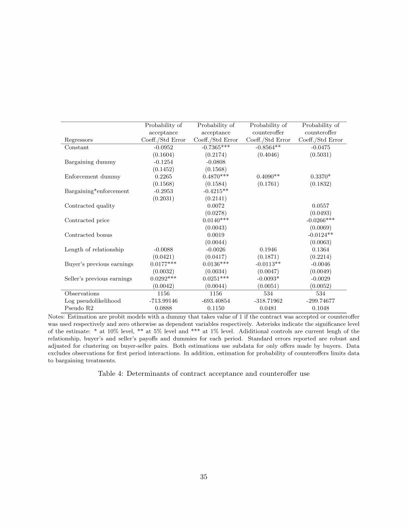
Probability of Probability of Probability of Probability ofacceptance acceptance counteroffer counteroffer

Regressors Coeff./Std Error Coeff./Std Error Coeff./Std Error Coeff./Std Error

Constant -0.0952 -0.7365*** -0.8564** -0.0475(0.1604) (0.2174) (0.4046) (0.5031)

Bargaining dummy -0.1254 -0.0808(0.1452) (0.1568)

Enforcement dummy 0.2265 0.4870*** 0.4090** 0.3370*(0.1568) (0.1584) (0.1761) (0.1832)

Bargaining*enforcement -0.2953 -0.4215**(0.2031) (0.2141)

Contracted quality 0.0072 0.0557(0.0278) (0.0493)

Contracted price 0.0140*** -0.0266***(0.0043) (0.0069)

Contracted bonus 0.0019 -0.0124**(0.0044) (0.0063)

Length of relationship -0.0088 -0.0026 0.1946 0.1364(0.0421) (0.0417) (0.1871) (0.2214)

Buyer’s previous earnings 0.0177*** 0.0136*** -0.0113** -0.0046(0.0032) (0.0034) (0.0047) (0.0049)

Seller’s previous earnings 0.0292*** 0.0251*** -0.0093* -0.0029(0.0042) (0.0044) (0.0051) (0.0052)

Observations 1156 1156 534 534Log pseudolikelihood -713.99146 -693.40854 -318.71962 -299.74677Pseudo R2 0.0888 0.1150 0.0481 0.1048

Notes: Estimation are probit models with a dummy that takes value of 1 if the contract was accepted or counterofferwas used respectively and zero otherwise as dependent variables respectively. Asterisks indicate the significance levelof the estimate: * at 10% level, ** at 5% level and *** at 1% level. Adiditional controls are current lengh of therelationship, buyer’s and seller’s payoffs and dummies for each period. Standard errors reported are robust andadjusted for clustering on buyer-seller pairs. Both estimations use subdata for only offers made by buyers. Dataexcludes observations for first period interactions. In addition, estimation for probability of counteroffers limits datato bargaining treatments.

Table 4: Determinants of contract acceptance and counteroffer use

35

Act

ual

Qu

alit

yS

oci

alS

urp

lus

Soci

alS

urp

lus

Soci

alS

urp

lus

Soci

alS

urp

lus

(los

str

ade)

(los

str

ade)

(ove

rall

loss

)(o

vera

lllo

ss)

Reg

ress

ors

Coeff

./S

tdE

rror

Coeff

./S

tdE

rror

Coeff

./S

tdE

rror

Coeff

./S

tdE

rror

Coeff

./S

tdE

rror

Con

stan

t-0

.403

519

.668

2***

7.87

99**

*18

.839

0***

7.29

24**

*(0

.636

4)(2

.166

6)(2

.003

)(2

.164

8)(2

.039

3)B

arg

ain

ing

du

mm

y1.

1337

*3.

9009

4.31

70**

1.28

442.

4791

(0.6

094)

(3.0

396)

(1.9

034)

(3.0

622)

(1.8

803)

En

forc

emen

td

um

my

0.49

242.

1623

0.49

532.

1387

0.50

25(0

.632

3)(3

.591

7)(2

.059

8)(3

.591

4)(2

.096

0)B

arg

ain

ing*e

nfo

rcem

ent

-1.3

136

-5.8

880

-4.8

275*

-4.8

664

-4.3

497

(0.8

308)

(4.4

912)

(2.7

237)

(4.4

654)

(2.6

641)

Len

gth

of

rela

tion

ship

0.11

451.

0631

0.56

250.

9995

0.52

34(0

.151

4)(0

.809

0)(0

.437

6)(0

.805

7)(0

.440

7)B

uye

r’s

pre

vio

us

earn

ings

0.12

50**

*0.

4831

***

0.47

04**

*(0

.013

8)(0

.049

6)(0

.049

8)S

elle

r’s

pre

vio

us

earn

ings

0.1

880*

**0.

7098

***

0.72

24**

*(0

.016

3)(0

.062

4)(0

.063

8)S

igm

a4.9

223*

**(0

.208

1)

Ob

serv

atio

ns

1156

1450

1156

1450

1156

Log

pse

ud

oli

keli

hood

-255

9.59

R-s

qu

ared

0.02

430.

2909

0.01

990.

2814

Note

s:T

he

esti

mati

on

for

act

ual

quality

isa

tobit

model

.T

her

ew

ere

421

left

-cen

sore

dobse

rvati

ons

at

0.

Est

imati

ons

for

soci

al

and

pri

vate

surp

lus

are

OL

Sw

ith

addit

ional

contr

ols

for

part

y’s

his

tory

inco

lum

ns

thre

eand

five,

whic

huse

data

rest

rict

edto

inte

ract

ions

aft

erp

erio

done.

Ast

eris

ks

indic

ate

the

signifi

cance

level

of

the

esti

mate

:*

at

10%

level

,**

at

5%

level

and

***

at

1%

level

.A

ddit

ional

contr

ols

incl

uded

dum

my

vari

able

sfo

r

each

per

iod.

Sta

ndard

erro

rsre

port

edare

robust

and

adju

sted

for

clust

erin

gon

buyer

-sel

ler

pair

s.A

llre

gre

ssio

ns

incl

ude

all

contr

act

soff

ered

.

Tab

le5:

Act

ual

qu

alit

y,so

cial

surp

lus

and

pri

vate

surp

lus

esti

mat

es(a

lloff

ers)

36

Act

ual

Qu

alit

yS

oci

alS

urp

lus

Soci

alS

urp

lus

Soci

alS

urp

lus

Soci

alS

urp

lus

(no

effici

ency

loss

)(n

oeffi

cien

cylo

ss)

(los

sb

arga

inin

g)(l

oss

bar

gain

ing)

Reg

ress

ors

Coeff

./S

tdE

rror

Coeff

./S

tdE

rror

Coeff

./S

tdE

rror

Coeff

./S

tdE

rror

Coeff

./S

tdE

rror

Con

stan

t3.0

463*

**30

.756

2***

18.7

183*

**29

.608

8***

17.9

190*

**(0

.135

6)(2

.062

8)(2

.136

1)(2

.100

3)(2

.190

1)B

arg

ain

ing

du

mm

y1.

3165

***

5.61

09**

6.06

55**

*1.

3165

3.06

12(0

.446

8)(2

.673

4)(2

.047

4)(2

.903

4)(2

.159

3)E

nfo

rcem

ent

du

mm

y-0

.410

8-0

.876

8-1

.753

6-0

.979

5-1

.799

7(0

.448

0)(3

.239

6)(2

.209

8)(3

.229

2)(2

.230

2)B

arg

ain

ing*e

nfo

rcem

ent

-1.0

840

-6.4

244

-4.6

811

-4.6

411

-3.8

662

(0.6

551)

(4.0

226)

(2.9

286)

(4.1

235)

(2.9

190)

Len

gth

of

rela

tion

ship

0.12

05**

*1.

3554

***

0.57

28**

*1.

2720

***

0.52

18**

*(0

.046

7)(0

.428

6)(0

.215

4)(0

.428

9)(0

.220

9)B

uye

r’s

pre

vio

us

earn

ings

0.10

03**

*0.

4546

***

0.43

90**

*(0

.011

2)(0

.048

8)(0

.051

6)S

elle

r’s

pre

vio

us

earn

ings

0.1

130*

**0.

5086

***

0.51

27**

*(0

.013

0)(0

.056

3)(0

.006

22)

Sig

ma

3.0

463*

**(0

.135

6)

Ob

serv

atio

ns

735

934

735

934

735

Log

pse

ud

oli

keli

hood

-1709

.236

3R

-squ

ared

0.04

410.

3361

0.03

380.

3041

Note

s:T

he

esti

mati

on

for

act

ual

quality

isa

tobit

model

.T

her

ew

ere

108

left

-cen

sore

dobse

rvati

ons

at

1.

Est

imati

ons

for

soci

al

and

pri

vate

surp

lus

are

OL

Sw

ith

addit

ional

contr

ols

for

part

y’s

his

tory

inco

lum

ns

thre

eand

five,

whic

huse

data

rest

rict

edto

inte

ract

ions

aft

erp

erio

done.

Ast

eris

ks

indic

ate

the

signifi

cance

level

of

the

esti

mate

:*

at

10%

level

,**

at

5%

level

and

***

at

1%

level

.A

ddit

ional

contr

ols

incl

uded

dum

my

vari

able

sfo

r

each

per

iod.

Sta

ndard

erro

rsre

port

edare

robust

and

adju

sted

for

clust

erin

gon

buyer

-sel

ler

pair

s.A

llre

gre

ssio

ns

incl

ude

only

com

ple

ted

contr

act

s.

Tab

le6:

Act

ual

qu

alit

y,so

cial

surp

lus

and

pri

vate

surp

lus

esti

mat

es

37

Sel

ler

payoff

sS

elle

rsh

are

Sp

read

inp

ayoff

sO

LS

Rob

ust

reg.

OL

SR

ob

ust

reg.

Qu

anti

le(5

0)

Qu

anti

le(9

0)

OL

SR

ob

ust

reg.

Qu

anti

le(5

0)

Qu

anti

le(9

0)

Reg

ress

ors

Coeff

./C

oeff

./C

oeff

./C

oeff

./C

oeff

./C

oeff

./C

oeff

./C

oeff

./C

oeff

.C

oeff

.S

tdE

rror

Std

Err

or

Std

Err

or

Std

Err

or

Std

Err

or

Std

Err

or

Std

Err

or

Std

Err

or

Std

Err

or

Std

Err

or

Con

stant

2.2

943

-3.1

721***

1.3

907***

0.4

666***

0.5

420***

4.2

034

***

-2.0

347***

0.0

312

-0.2

063***

3.0

419***

(2.6

694)

(0.9

277)

(0.3

365)

(0.0

376)

(0.0

234)

(0.0

709)

(0.6

687)

(0.0

759)

(0.0

293)

(0.2

027)

Barg

ain

ing

du

mm

y1.1

232

3.4

486***

0.0

014

0.1

442***

0.0

387**

0.0

133

-0.3

233

-0.3

070***

-0.1

352***

-0.2

368

(2.3

729)

(0.7

823)

(0.1

803)

(0.0

317)

(0.0

194)

(0.0

553)

(0.3

465)

(0.0

640)

(0.0

244)

(0.1

693)

En

forc

emen

td

um

my

2.1

148

2.4

420***

0.3

450**

0.0

410

0.0

387**

0.0

163

-0.6

897**

-0.0

815

-0.1

352***

-1.2

664***

(1.6

653)

(0.6

846)

(0.1

677)

(0.0

278)

(0.0

170)

(0.0

502)

(0.3

413)

(0.0

560)

(0.0

215)

(0.1

347)

Barg

ain

ing*en

forc

emen

t3.6

011

-0.7

058

0.3

063

0.0

492

0.0

924***

0.1

692**

-0.3

004

-0.0

817

-0.0

979***

-0.1

461

(2.5

486)

(1.0

160)

(0.2

247)

(0.0

412)

(0.0

253)

(0.0

753)

(0.4

353)

(0.0

832)

(0.0

318)

(0.2

185)

Act

ual

qu

ality

0.6

810***

2.1

524***

-0.1

718***

-0.0

145***

-0.0

206***

-0.3

696***

0.3

539***

0.0

310***

0.0

571***

-0.0

407**

(0.2

549)

(0.0

870)

(0.0

314)

(0.0

035)

(0.0

022)

(0.0

092)

(0.0

624)

(0.0

071)

(0.0

027)

(0.0

191)

Bu

yer

pre

vio

us

earn

ings

0.0

573

0.0

712***

-0.0

002

0.0

002

-0.0

022***

-0.0

074***

0.0

029

-0.0

004

0.0

058***

-0.0

111*

(0.0

560)

(0.0

182)

(0.0

049)

(0.0

007)

(0.0

005)

(0.0

017)

(0.0

098)

(0.0

015)

(0.0

006)

(0.0

059)

Sel

ler

pre

vio

us

earn

ings

0.3

710***

0.0

851***

0.0

217***

0.0

027***

0.0

075***

0.0

100***

-0.0

407***

-0.0

048***

-0.0

151***

-0.0

226***

(0.0

724)

(0.0

206)

(0.0

062)

(0.0

008)

(0.0

005)

(0.0

018)

(0.0

124)

(0.0

017)

(0.0

006)

(0.0

058)

Len

gth

of

rela

tion

ship

0.0

612

-0.0

710

0.0

225

-0.0

004

-0.0

029

0.0

000

-0.0

551

0.0

000

0.0

018

0.0

000

(0.1

926)

(0.2

131)

(0.0

212)

(0.0

086)

(0.0

053)

(0.0

124)

(0.0

435)

(0.0

174)

(0.0

068)

(0.0

258)

Ob

serv

ati

on

s735

735

735

735

735

735

735

735

735

735

R-s

qu

are

d0.1

659

0.1

544

0.1

603

Pse

ud

oR

20.0

223

0.2

543

0.0

237

0.1

757

Note

s:C

olu

mns

one,

thre

eand

seven

are

OL

Ses

tim

ati

ons

wit

hse

ller

’spay

off

,se

ller

’ssh

are

and

pay

off

spre

ad

as

dep

enden

tva

riable

sre

spec

tivel

y.C

olu

mns

two,fo

ur

and

eight

are

robust

regre

ssio

ns

for

the

sam

edep

enden

tva

riable

s.C

olu

mns

five,

six,nin

eand

ten

are

med

ian

and

90

per

centi

lere

gre

ssio

ns

resp

ecti

vel

y.A

ster

isks

indic

ate

the

signifi

cance

level

of

the

esti

mate

:*

at

10%

level

,**

at

5%

level

and

***

at

1%

level

.A

ddit

ional

contr

ols

are

quality

level

del

iver

ed,

the

curr

ent

lengh

of

the

rela

tionsh

ip,

buyer

and

seller

pay

off

sand

dum

mie

sfo

rea

chp

erio

d(n

ot

incl

uded

inoutp

ut)

.Sta

ndard

erro

rsre

port

edare

robust

and

adju

sted

for

clust

erin

gon

buyer

-sel

ler

pair

sfo

rth

eO

LS

esti

mati

ons.

Tab

le7:

Dis

trib

uti

onal

outc

omes

38

0

0.1

0.2

0.3

0.4

0.5

0.6

1 2 3 4 5 6 7 8 9 10 11 12

Proportion counteroffers PB Proportion counteroffers NB

Potential profits (scale)_NB Potential profits (scale)_PB

Period

Figure 5: Number of counteroffers and potential sellers’ profits in offers

39

Contracted Price Contracted BonusRegressors Coeff./Std Error Coeff./Std Error

Constant 20.1102*** 26.7579***(2.8792) (3.0905)

Bargaining dummy 10.2022*** -5.1524(2.8023) (3.2583)

Length of relationship 1.0240* -1.1720*(0.5811) (0.6580)

Buyer previous earnings 0.3931*** 0.0740(0.0925) (0.1053)

Seller previous earnings 0.4701*** -0.0226(0.0955) (0.0882)

p3 -4.9348** 3.7702(2.1578) (2.4724)

p4 -5.5992** 1.3222(2.3906) (2.4458)

p5 -5.2252 5.4539(3.6098) (4.0222)

p6 -12.3600*** 9.6626**(4.2306) (4.6904)

p7 -9.6331* 9.6618(5.5954) (6.5043)

p8 -15.4979** 21.8971**(6.0232) (9.0065)

pl -12.9785* 12.6187(6.7161) (8.7038)

Sigma 16.4522*** 18.3279***(0.9842) (1.3839)

Observations 411 411Log pseudolikelihood -1725.3486 -1731.1145Pseudo R2 0.0311 0.0066

Notes: The estimations are tobit models and used observations from period 2 and above. Total pay-

ment regression used data from all treatments and had 34 left-censored observations at 0; price and

bonus regressions used data only from partial enforcement treatments and have 3 and 149 left-censored

observations at 0 respectively. Asterisks indicate the significance level of the estimate: * at 10% level,

** at 5% level and *** at 1% level. Standard errors reported are robust and adjusted for clustering on

buyer-seller pairs. Additional controls include period dummies in which pl is a dummy for period 9 and

above.

Table 8: Bargaining effect in contract structure

40

Appendix

This appendix presents technical details about the experimental design. Each treatment was run

in four sessions except the PB treatment, which was run in five sessions.

Matching procedure: Subjects were matched into pairs by using a rotation matching scheme.

In each session, subjects were randomly divided into two groups: buyers and sellers. In each match,

every buyer was paired with a seller and subjects were not paired with each other more than once.

Moreover, the pairing was done in such a way that the decisions made by one subject in one

match could not affect them in any future match interactions. These features were explained to

the participants. Because subjects were matched with each other only once, the total number of

possible matches per session is N/2, where N is the number of subjects attending a session.

Infinitely repeated games: In each treatment, a random termination rule was used to induce

infinitely repeated games. The probability of continuation used was δ = 4/5, which was the same

for all treatments. In each trading period the supergame is expected to go on for 5 additional

periods.7 This was done at the end of each trading period by having the computer draw a number

between 0 and 1, using a uniform distribution. The supergame terminated if the computer draw was

0.81 or higher. This randomization mechanism generates a infinitely repeated game because there

is always a possibility of interacting with the same subject in the next round. The probability of

continuation allows us to control for the subjects’ beliefs regarding the probability of continuation

as subjects played a game with an uncertain number of trading periods. Because of the random

termination rule, each supergame may have a different number of periods but all supergames have

the same expected duration of five rounds. Then, each experimental session may be formed of one

long-duration supergame or various short-duration supergames of the same treatment with different

partners depending on the random termination rule. The number drawn by the computer serves as

a public randomization device as in all sessions all participants observe the same drawn number.

Stage game payoffs: The stage game payoffs differ among bargaining and no bargaining

treatments. In the bargaining treatments, I include in the payoff functions the parameter β from the

7The expected number of periods of a game with a continuation probability of δ is equal to T = 11−δ

. Therefore,with δ = 4/5 the expected number of periods each pair interacts equals 5.

41

theroretical model. The parameter reflects the bargaining power which in the traditional alternating

offer game is the cost of delaying trade. In the experiments it serves as a way to transfer bargaining

power between players by not only giving the opportunity to the seller to counteroffer but also by

inflicting an asymmetric cost of delay for parties.

Implementation of the bargaining: To implement the difference in bargaining power in the

experiment, the design included two different conditions. In the first condition the buyer made

a take-it-or-leave-it offer to the seller who could only accept or reject – in essence an ultimatum

game. In the second condition, the seller was able to make a counteroffer if he or she rejected the

buyer’s offer–an alternating offer game with two offers and an asymmetric cost for delaying trade

for each party.

Subjects’ total earnings: All payoffs were in points. At the end of each session, the points

earned by each subject were converted into dollars at the exchange rate of 50 points= $1. Subjects

were paid privately the equivalent of points earned plus the money resulting from a pre-experimental

gamble that the subjects had the option to play by using their show-up fee of $8. Note the resolution

of this gamble did not occur until the end of the session.

Order of treatments: Subjects could participate in only one session and each subject played

only a single treatment. Therefore, there was no possibility of spillover effects from one treatment

to another.

Throughout the pre-experimental activities subjects neither received feedback about their

decisions nor information about other subjects’ decisions. They were not informed about their own

payoffs until the end of the experiment. Subjects were informed about these procedures, and they

were also aware that their decisions in the pre-experimental activities were completely independent

of the trading game.

Summary statistics. Offer fraction shows the proportion of possible interactions in which a

buyer made an offer. Acceptance rate fraction shows the proportion of those offers accepted by

the seller. Counteroffer fraction shows the proportion of all possible interactions that resulted in a

counteroffer and Counteroffer after rejection fraction shows the proportion of rejected offers that

were followed by a counteroffer. Counteroffer acceptance rate shows the proportion of those coun-

42

teroffers accepted by buyers. Number of pairs shows the number of distinct subjects pairs. Average

length of the relationship shows how many periods each pair interacted. Pairs used offer, fraction

and Pairs used counteroffer, fraction show the proportion of pairs that used offers and counteroffers

respectively while Pairs contracted by offer, fraction and Pairs contracted by counteroffer, fraction

show the proportion of pairs that agreed on a contract by using offers or counteroffers respectively.

Av. proposed quality and Av. proposed payment show the average for all contracts that were pro-

posed regardless if they were accepted or not. Av. proposed quality (offers, Av. proposed payment

(offers), Av. proposed quality (counteroffers) and Av. proposed payment (counteroffers) show the

average regardless of acceptance or rejection but for contracts proposed as offer and as counteroffers

respectively.

The remaining variables in Table 2 are restricted to the actual contracts that were accepted

including offers and counteroffers. Average contracted quality and Average contracted payment

show the averages specified in the accepted offers and counteroffers, while Average actual quality

and Average actual payment show the averages actual delivered by both the seller and buyer

respectively. Average buyer payoffs and Average seller payoffs and Median seller payoffs are the

average and median seller earnings in points per period. Overall seller share and Overall seller share

(median) show the mean and median proportion of the private surplus (sum of parties’ payoffs)

captured by the seller including all contracts respectively, while Seller share if offer and Seller

share if counteroffer show the proportion of the surplus captured by the seller when the contract

was reached by an offer or counteroffer respectively. Trunc. seller share is similar to overall seller

share but it truncates the ratio of payoffs to total available private surplus to the unit interval. In

this case, if the payoff of either party is negative, the share is set to 0 and the other party’s share

is set to one. Payoffs relative spread presents another way of looking at surplus distribution. It is

the ratio of the spread between buyers’ and sellers’ payoffs to the total available private surplus.

Finally, the Cooperation rate shows the overall average cooperation which is defined as pairs that

act according to the contract while Cooperation rate if offer and Cooperation rate if counteroffer

show the average cooperation when the contract was achieved through an offer and counteroffer

respectively.

43

NB NN PB PN

4.04a 4.94a,b 4.96b,c 6.52c

Notes: Different letter superscripts in-

dicate that numbers are statistically

distinct.

Table 9: Average number of periods per match

Tests for effects Because the experiments mimic the infinite repetition of the theoretical

model, the realized durations varied considerably and subjects play games with different lengths.

The number of played rounds may impact subject’s decisions. A Mann-Whitney tests give evidence

that the number of periods played per match is significantly different between some treatments

(Table 9 presents the average number of periods per match). Therefore, I control for the length of

the relationship in the econometric analysis.

In addition, because subjects may learn throughout the experiment, subjects’ behavior may

be substantially different from the theoretical equilibrium in earlier periods, but, over time sub-

jects adjust their choices and converge to the theoretical equilibrium. As a consequence potential

differences across treatments may be due to learning effects, especially between those that have

significantly different length.

To explore if this is an issue, I test for learning effects across games, for each treatment and

early and later periods across treatments. First, I compare subjects’ decisions across the games

played in each single session across treatments.8 I find a significant difference in the mean values

of the most relevant variables between some of the games (superscripts in table 10 ). This evidence

suggests that subjects’ early behavior differs somewhat from later behavior.

Furthermore, subjects became more familiar with the incentive structure of the indefinite

repetition across games in the same sessions. Figure 6 shows the learning trend in cooperation

between games across treatments. Participants increase cooperation from the first two games to

the later games. Even though cooperation is lower in game 5, it is not statistically different than

cooperation in game 4. However, the difference in cooperation among games is significant at 5%

level (Kruskal-Wallis test).

8Because of the use of a random termination rule, one or more games were played in each session. Then, the gamenumber represents the order in which the game was played in a session (first, second, third, etc.).

44

Variable Game 1 Game 2 Game 3 Game 4 Game 5N=934 n=252 n=200 n=246 n=161 n=75

Av. contracted quality 7.53a 7.58a,b 8.37c 8.58c,d 7.89b,c,d

Av. actual quality 6.08a 5.53a,b 6.89c 7.68d 6.63c,d

Av. contractual payment 58.09a 59.05a,b 63.83c 63.88c,d 64.43c,d

Av. actual payment 44.33a 40.34a,b 49.75c 55.21d 50.84c,d

Av. seller’s payoffs 13.89a 12.46a,b 15.17a,c 16.77c,d 17.66c,d

Av. buyer’s payoffs 15.02a 13.66a,b 17.34a,c 21.38d 12.78b,c

Cooperation rate 0.36a 0.32a,b 0.44a,c 0.53c,d 0.40b,c,d

Av. Surplus 30.40a 27.63a,b 34.47c 38.42d 33.13c,d

Private Av. Surplus 28.91a 26.11 32.51b 38.15 30.43a,b

Notes: Numbers within a row with different letter superscripts are statistically distinct according

to pairwise Mann-Whitney tests. Differences among games are statistically significant at 1% or 5%

levels .

Table 10: Mean values per game across treatments

When I test for learning effects within each individual treatment, I find that the no enforce-

ment treatments present some significant increasing differences among games for desired quality,

actual quality, desired total payment, cooperation and surplus. This evidence suggests that the

small learning trend observed in the overall analysis is driven by the no enforcement treatments,

especially by the NN treatment where learning trends are significant at the 1% level for almost

all variables. I also compare the means of the variables of interest among early and later periods

across treatments and for each treatment. The analysis gives evidence of learning trends in sub-

ject behavior. As in the previous analysis, the presence of learning effects is stronger in the NE

treatments than in the PE treatments. Therefore, I control for learning effects in the econometric

analyses.

A final consideration is the difference in the number of periods played among games. In the

NB treatment the longest game had 9 periods while in the NN, PB and PN treatments the longest

game had 17, 12 and 20 periods respectively. I test for potential differences among treatments

because of the presence of longer games. By using the pooled data for all treatments, I find a sig-

nificant difference in the total payment (MW test p=0.0410), sellers’ profits (MW test p=0.0604)

and cooperation (MW test p=0.0102). When I analyze the differences among sessions for indi-

vidual treatments, I only find significant differences in the NN treatment. Therefore, I include all

45

0.36

0.32

0.44

0.44

0.40

.2.3

.4.5

.6M

ean

coop

erat

ion

rate

1 2 3 4 5Game number

Cooperation (mean) Confidence interval

Figure 6: Average cooperation across games in all treatments

observations in the analysis and I control for potential differences due to longer games by including

dummy variables for each period.

46

References

Brown, M., A. Falk, and E. Fehr, “Relational Contracts and the Nature of Market Interac-tions,” Econometrica, 2004, 72, 747–780.

Fischbacher, U., “Z-Tree: Experimental Software,” Technical Report, University of Zurich. 1999.

Guth, Werner, Rolf Schmittberger, and Bernd Schwarze, “An experimental analysis ofultimatum bargaining,” Journal of Economic Behavior & Organization, 1982, 3(4), 367–388.

Iskow, J. and R. Sexton, “Bargaining Associations in Grower-Processor Markets for Fruits andVegetables,” Technical Report, Department of Agricultural Economics, University of California,Davis 1992.

Kagel, John H., Chung Kim, and Donald Moser, “Fairness in Ultimatum Games withAsymmetric Information and Asymmetric Payoffs,” Games and Economic Behavior, 1996, 13(1), 100–110.

Lee, Jason, “Are Health Insurance Premiums Higher for Small Firms?,” Technical Report, TheRobert Wood Johnson Foundation 2002.

Lee, Myoungki, Seteven Y. Wu, and Maoyong Fan, “Balancing Grower Protection AgainstAgency Concerns: An Economic Analysis of Contract Termination Damages,” Journal of Agri-cultural and Reciurces Economics, 2008, 33(2), 154–168.

Levin, J., “Relational Incentive Contracts,” American Economic Review, 2003, 93, 835–847.

Love, H.Alan and Diana M. Burton, “A Strategic Rationale for Captive Supplies,” Journalof Agricultural and Resource Economics, 1999, 24(1), 1–18.

MacDonald, James, Janet Perry, Mary Ahearn, David Banker, William Chanbers,Carolyn Dimitri, Nigel Key, Kenneth Nelson, and Southard Leland, “Contracts, Mar-kets, and Prices: Organizing the Production and Use of Agricultural Commodities,” TechnicalReport, USDA 2004.

Ochs, J. and A. Roth, “An Experimental Study of Sequential Bargaining,” American EconomicReview, 1989, 79, 355 – 384.

Prasnikar, Vesna and Alvin E Roth, “Considerations of Fairness and Strategy: ExperimentalData from Sequential Games,” The Quarterly Journal of Economics, 1992, 107(3), 865–88.

Roth, Alvin E and J Keith Murnighan, “The Role of Information in Bargaining: An Experi-mental Study,” Econometrica, 1982, 50(5), 1123–42.

Salas, Paula Cordero, “The Role of Bargaining Power in Agricultural Contracts,” Available atSSRN: http://ssrn.com/abstract=1344550, 2011.

the Democratic Staff, “Economic Concentration and Structural Change In the Food and Agri-culture Sector: Trends, Consequences and Policy Options,” Technical Report, Technical Report,Committee on Agriculture, Nutrition, and Forestry United States Senate. 2004.

47

Wu, S. Y. and B. Roe, “Contract Enforcement, Social Efficiency, and Distribution: SomeExperimental Evidence,” American Journal of Agricultural Economics, 2007, 89, 243–258.

and , “Discretionary Latitude and Relational Contracting,” Technical Report, IZA DiscussionPaper No. 2879 Available at SSRN: http://ssrn.com/abstract=999376 2007.

Wu, S.Y., “Contract theory and agricultural policy analysis: a discussion and survey of recentdevelopments,” Australian Journal of Agricultural and Resource Economics, 2006, 50, 490–509.

48