Documentos de Trabajo N.º 1020

I.T. INVESTMENT AND INTANGIBLES: EVIDENCE FROM BANKS

Alfredo Martín-Oliver and Vicente Salas-Fumás

Documentos de Trabajo N.º 1020

2010

I.T. INVESTMENT AND INTANGIBLES: EVIDENCE FROM BANKS

I.T. INVESTMENT AND INTANGIBLES: EVIDENCE FROM BANKS (*)

Alfredo Martín-Oliver (**)

BANCO DE ESPAÑA

Vicente Salas-Fumás

UNIVERSIDAD DE ZARAGOZA

(*) This paper is the sole responsibility of its authors and the views represented here do not necessarily reflect those of the Banco de España. Any errors are entirely the authors’ own responsibility. We thank three anonymous referees for their comments to a previous version of the paper. V. Salas-Fumás acknowledges the financial support from project SEJ 2007-67895-C04-04.

(**) Address for correspondence: Alfredo Martín-Oliver; c/Alcalá, 48, 28014 Madrid, Spain. Tlf: + 34 91 338 6178; Fax: + 34 91 338 6102; e-mail: [email protected].

Documentos de Trabajo. N.º 1020

2010

The Working Paper Series seeks to disseminate original research in economics and finance. All papers have been anonymously refereed. By publishing these papers, the Banco de España aims to contribute to economic analysis and, in particular, to knowledge of the Spanish economy and its international environment. The opinions and analyses in the Working Paper Series are the responsibility of the authors and, therefore, do not necessarily coincide with those of the Banco de España or the Eurosystem. The Banco de España disseminates its main reports and most of its publications via the INTERNET at the following website: http://www.bde.es. Reproduction for educational and non-commercial purposes is permitted provided that the source is acknowledged. © BANCO DE ESPAÑA, Madrid, 2010 ISSN: 0213-2710 (print) ISSN: 1579-8666 (on line) Depósito legal: M. 30124-2010 Unidad de Publicaciones, Banco de España

Abstract

This paper models the investment behaviour of a multi-asset firm with market power that

accumulates valuable intangible assets to complement the IT capital. The investment model

is estimated using data from Spanish banks on assets of different nature: material (branches,

financial), immaterial (advertising and IT) and intangible (training of workers). The paper

estimates that the representative bank spends five additional Euros per Euro invested in

IT-related assets in complementary intangible assets or, equivalently, intangibles amount

to approximately 10% of the economic value of the representative bank. The remaining

economic value is distributed between 28% from rents attributed to market power, and 62%

to the cost of market-purchased assets.

Keywords: multi-asset firm; investment; intangible assets; banks.

JEL: G21; D92

BANCO DE ESPAÑA 9 DOCUMENTO DE TRABAJO N.º 1020

1 Introduction

Intangible assets have received increasing recognition as sources of the economic value of

individual firms [Lev (2001); Brynjolfsson, Hitt and Yang (2002); Hulten and Hao (2008)] and as

sources of countries’ economic growth [Buiges, Jacquemin, Marchipont (2000); Corrado,

Haltiwanger, Sichel (2005); Corrado, Hulten and Sichel (2009); Marrano, Haskel and Wallis

(2009), Fukao et al. (2009)]. Assets identified as intangibles are not homogenous, and their

measurement raises controversies. Most often, intangibles refer to immaterial assets, such as

those resulting from R&D, advertising and information technology (IT) expenditures. However,

intangible assets are also defined, in a more restrictive way, as the assets that firms build

up internally as a sub-product of their regular activities, such as production of goods and/or

investment in market-purchased assets. Examples of the latter are the “organizational capital” of

Prescott and Visscher (1980) and the “organization capital” of Brynjolfsson, Hitt and Yang (2002)

and Lev and Radhakrishnan (2005).1 Both immaterial and intangible assets are most often

registered as expenses of the year by conventional accounting practices, even though these

expenditures increase future consumption opportunities and they could be justified being

accounted as investments [Blair and Wallman (2001); Corrado, Hulten and Sichel (2009);

Corrado, Haltiwanger and Sichel (2005)].

Different approaches have aimed to obtain a measure of the unreported intangible

assets of firms, though they present several caveats. The approach of measuring the amount of

intangible assets as the difference between market and book value of the firm [Hall (2001) and

Villalonga (2004)] does not separate the cost of investment in the assets and the economic value

that those assets contribute to create (economic rents).2 The use of expenditures reported in

separate lines of the income statement to obtain estimates of the stock of intangibles [a practice

going back to Griliches (1981)], common in macro-economic analysis [Corrado, Hulten and

Sichel (2009); Marrano, Haskel and Wallis (2009), Fukao et al. (2009)], abstracts from the ex-ante

investment decision process of the firms, and does not make an explicit distinction between

market-purchased assets and assets resulting from production and/or investment activities, such

as organization capital. Oliner, Sichel and Stiroh (2007) use the model proposed by Basu, Oulton

and Srinivasan (2003) to obtain estimates of intangible capital related to IT. In this model, the IT

capital and the intangibles are complementary assets that are combined to generate flows

services used as inputs of the production function of the firm. Assuming that firms choose the

mix of IT and intangibles in an efficient way, the growth of the (invisible) stock of intangibles can

be estimated as a function of the growth of the (observable) IT capital. Nonetheless, the model

does not explicitly link intangibles with the outcome of adjustment costs, nor does it consider the

possibility of market power of banks. Finally, hedonic-price approaches to measuring the value of

intangible assets [Cockburn and Griliches (1988), Hall (1993)] estimate the marginal contribution

of each asset to the value of the firm, tangible and intangible, but do not separate the estimated

marginal contribution in purchase costs, adjustment costs (that may turn into organization

capital) and contribution in the form of rents, from market power.

1. Lev and Radhakrishnan (2005) and Cummins (2004) say that the word intangibles should be used only to refer to built-in

intangibles, such as organization capital. In this paper, we make a distinction between immaterial (advertising, and IT

purchased in the market) and intangibles.

2. Another problem is that the market price of the shares of firms may be affected by bubbles, and other possible

inefficiencies, causing a deviation between the market and the fundamental value of the firm.


This paper proposes an ex-ante decision model of the investment behaviour of a multi-

asset firm that provides a comprehensive approach to the valuation of the firm and of all its

invested assets. The results of the model are empirically applied to data from Spanish banks for

the period 1984-2003, to obtain estimates of the value of the stock of intangible assets built in

the process of investing in IT capital. Recent research on the so-called “IT revolution” and “new

economy” has called attention to how advances in IT opened the way to new work processes,

new job definitions and new management functions in firms of all economic sectors. The new

business models lowered the costs of the old activities and allowed firms to implement new ones

[Brynjolfsson, Hitt and Yang (2002)]. In this paper, we have grouped all these capabilities,

resulting from investment and use of IT-related assets, under the “organizational capital” of the

firm. Therefore, our approach to the measurement of intangibles makes an explicit distinction

between market-purchased immaterial assets (advertising and IT capital) and intangibles that are

internally generated as a sub-product during the process of making IT capital fully productive.

With the data available for each bank on expenditures in training workers, we obtain estimates of

the part of the adjustment costs that become intangible assets. These intangible assets are a

part of the human capital that enables workers to use computers more efficiently [Bresnahan,

Brynjolfsson and Hitt (2002)]. Finally, we split the value of intangibles into their cost of

accumulation, and the value of the rents from market-power that these intangibles may generate.

The theoretical model is drawn from the theory of investment of a multi-asset firm that

maximizes its economic value subject to adjustment costs of growth [Wildasin (1984); Hayashi

and Inoue (1991); Brynjolfsson and Yang (1999); Bond and Cummins (2000)]. We extend the

basic model in two ways: i) firms have market power; and ii) the intangible assets that firms build

in the process of making IT capital productive (organizational capital) contribute positively to the

profits of the firm.3 Bond and Cummins (2000) modelled and estimated the investment equation

for the multi-asset firm, but assumed perfect competition and do not explicitly relate adjustment

cost from IT assets accumulation with the outcome in the form of organizational capital.

Brynjolfsson and Yang (1999) and Cummins (2004) link the adjustment costs from IT investment

with built-in intangibles, but they model the valuation equation of the firm (not the investment

equation, as we do in this paper), they assume perfect competition, and they do not make

explicit the contribution of the built-in intangibles to profits.

In the empirical application, the paper uses estimates of the stock of several

market-purchased assets valued at replacement cost: material assets (branches and equipment),

immaterial assets (advertising and IT capital), financial assets, and human capital (from training).

The theory predicts that, if the adjustment costs (such as the costs of training workers to use

computers) turn into valuable intangible assets, then the estimated adjustment cost of investing

in IT capital will be decreasing with the marginal economic value of these intangibles. The other

prediction (related to the extensions of the investment model) states that banks with market

power will invest at a lower rate than banks with no market power. The empirical estimations of

the investment equation for the multi-asset bank do a good job in explaining the value-

maximizing investment behaviour of Spanish banks. The empirical results confirm that human

capital from training workers is an intangible asset built in the process of investing in IT that

contributes to the economic value of the bank. Finally, the results also confirm that banks have

market power, especially in the deposits market. The assets that seem to contribute to market

3. Market power can be interpreted as a hidden cost of growth, since it implies that as firms expand capacity they will lower

future revenues of output from current capacity, since they will have to lower the price as a way to increase demand. This

cost has been considered in single-asset investment models based on Euler’s equations [Schiantarelly and Georgoutsos

(1990), Bond and Meghir (1994)].


power are advertising capital and (marginally) intangibles (no evidence is found of a contribution

for IT, physical or financial assets).4

To our knowledge, this is the first application of the multi-asset Tobin’s q investment

model to banks, and also the first to study in depth the process of IT investment and intangibles

in the banking industry. The distinct feature of the banking firm in the model is that the

investment in financial assets, which is one of the explanatory variables of the investment

equation, can be used to infer possible restraints on the banks in satisfying their requirements of

regulatory capital. The empirical analysis finds no evidence of such restraints, probably because

the time period considered in this study has been relatively favourable in terms of macro-

economic conditions, and banks have been able to meet their solvency requirements without

major difficulty.

The rest of the paper is organized as follows. In Section 2, we present the derivation

and interpretation of the investment function for the multi-asset bank. In Section 3, we present

the description of the database, the results of the empirical estimation of the investment equation

using data from Spanish banks, and a discussion of the results. The conclusion summarizes the

main results of the paper.

4. Besides the debate on whether IT investment turns into intangible assets or not [see for example the different views on this

issue by Brynjolfsson, Hitt and Yang (2002) and Cummins (2004), there is another debate on whether IT-related assets give a

competitive advantage to firms, so that investment in IT turns into economic rents [Bharadwaj, Bharadwaj and Konsynski

(1999)] or not [Carr 2003)]. See Beccalli (2007) for an empirical analysis of the relationship between IT investment and the

profitability of banks, using accounting data.


2 The investment model

2.1 Hypotheses

We consider a bank that issues equity to finance the assets needed to produce and deliver

banking services, and also to satisfy the minimum regulatory equity requirements.

The economically optimal volume of equity on the liability side of the balance sheet of the bank

will then be equal to the sum of the stocks of physical assets, IT-related assets, advertising

capital (operating assets of the bank), and the stock of financial assets, all on the asset side of

the balance sheet. We do not model the choice of the capital ratio of the bank, but consider that

banks’ equity always satisfies the minimum capital requirements set by regulation. From these

assumptions, we can focus on the optimal decisions concerning resources that are the

counterpart to the equity on the asset side of the balance sheet, including the financial assets. In

this section, we formulate the model that determines the investment equation for a general firm

with N different assets, assuming that the firm has market power, and that there is one asset for

which adjustment costs turn into valuable intangible assets (organizational capital).

In each time period, the firm/bank decides how much to invest in each type of N different

market-purchased capital goods, It = (I1t, I2t,…,INt). The firm holds a stock of capital services at the

beginning of the period t, Kt-1=(K1t-1,…,KNt-1) that changes over time as the result of new

investments and of the depreciation of old ones,

0and M 1,....,jfor 1 ,1,, sIKK stjstjjstj (1)

where j is the depreciation rate of capital asset j.

To make fully productive the new invested assets, the firm has to incur adjustment costs.

Let C(.) be the adjustment cost function that is assumed separable in the adjustment costs of

each of the assets in which the firm invests,

jjj

j

jjj

jjjjss Ka

K

IbpIKCIKC

2

2,),( (2)

where bj is a positive (cost) parameter and aj is the stationary investment rate for which

adjustment costs are zero (in general equal to the depreciation rate), and pj is the market

purchase price of one unit of asset j. The adjustment cost function is defined in Euros of new

investments that do not turn into capital stock of the respective productive asset.5

The new assumption introduced in the paper is that the adjustment costs incurred

in certain investments are accumulated into a valuable intangible asset (valuable

because it positively affects the cash flow of the firm). In the paper, sub-index k identifies

the assets whose investments imply building complementary intangible assets. In the empirical

analysis, k will be limited to IT capital and the associated intangibles are, among others, those

accumulated in the form of human capital from training workers in the use of computers, and

related assets. Let Mk be the stock of intangible assets resulting from expenditures in the form of

5. Although it would be realistic to assume a non-separable adjustment cost function, for simplicity, we maintain the

assumption of separable adjustment cost functions.


adjustment costs associated with the market- purchased asset k. The stock Mk will vary over

time as the net result of depreciation and the flow of new intangibles from current expenses in

adjustment costs, Ck:

)(1 1, tktkkkt CfMxM (3)

where xk is the depreciation rate of the intangible assets and f (Ckt) is the flow of intangibles

produced with the adjustment costs incurred in period t, which in turn depends on Ik and Kk [from

equation (2)] We assume that f ( ) increases with the expenditures in adjustment costs, Ck.

Let (Ks, Mks, Is, es) be the net cash flow of the firm in period s as a function of the stock

Ks and the investment flow Is of the assets in the period, and of the random productivity shock es,

once the non-capital inputs used in the production, for example labour, are optimized. The stock

of intangible asset M enters the cash flow function because it is assumed to be a valuable asset.

The cash flow function has three separate components: gross revenues from operations,

adjustment costs, and the outlay from current market-purchased assets:

j

jsjssssksssskss IpIKCeMKReIMK ,,,,,,

Gross revenue R(.) is in turn equal to the price times the quantity of product sold, R(.) = p

(Q (Ks,Mks)) Q(Ks,Mks), where price is non-increasing with the quantity sold (i.e. firms can have

market power); pjs is the current market purchase price of one unit of capital asset j, and C(.) is

given by (2).

The economic value of the firm in period t, Vt, will be equal to the present value of

expected future cash flows,

tssskss

tstt eIMKEV ,,, (4)

where Et is the expectations operator, conditional on the information available at the beginning of

period t, and ts is the discount factor.

The optimization problem of the firm is to choose I, K and M such that (4) is maximized

subject to (1), (2) and (3). The detailed solution to this problem is presented in Appendix A. Here,

we focus on the two equations that result from the optimization:

sts

stsktkt

jjtjtjtt KQKQpMzIKV

)(1

(5.1)

'Ijtjtjt Cp if j≠k

'''IktCktIktktkt CfzCp

k if j=k

(5.2)

where jt and zkt are the Lagrange multipliers for constraints (2) and (3), respectively, and C’Ijt

is the marginal adjustment cost for the investment flow in asset j [derivative with respect to

investment flow of the adjustment cost function (2)].


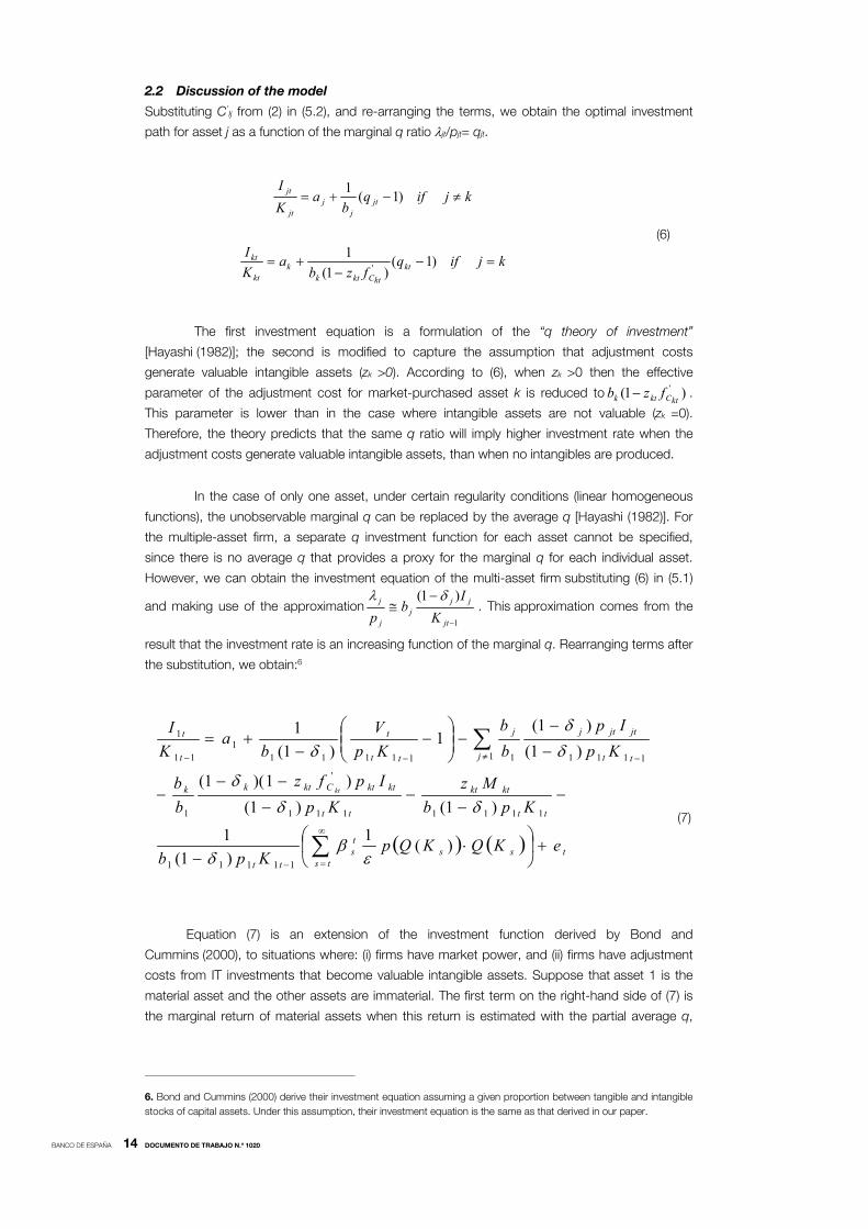
2.2 Discussion of the model

Substituting C’Ij from (2) in (5.2), and re-arranging the terms, we obtain the optimal investment

path for asset j as a function of the marginal q ratio jt/pjt= qjt.

kjifqb

aK

Ijt

jj

jt

jt )1(1

kjifqfzb

aK

Ikt

ktCktkk

kt

kt

)1()1(

1'

(6)

The first investment equation is a formulation of the “q theory of investment”

[Hayashi (1982)]; the second is modified to capture the assumption that adjustment costs

generate valuable intangible assets (zk >0). According to (6), when zk >0 then the effective

parameter of the adjustment cost for market-purchased asset k is reduced to )1( 'ktCktk fzb .

This parameter is lower than in the case where intangible assets are not valuable (zk =0).

Therefore, the theory predicts that the same q ratio will imply higher investment rate when the

adjustment costs generate valuable intangible assets, than when no intangibles are produced.

In the case of only one asset, under certain regularity conditions (linear homogeneous

functions), the unobservable marginal q can be replaced by the average q [Hayashi (1982)]. For

the multiple-asset firm, a separate q investment function for each asset cannot be specified,

since there is no average q that provides a proxy for the marginal q for each individual asset.

However, we can obtain the investment equation of the multi-asset firm substituting (6) in (5.1)

and making use of the approximation1

)1(

jt

jjj

j

j

K

Ib

p

. This approximation comes from the

result that the investment rate is an increasing function of the marginal q. Rearranging terms after

the substitution, we obtain:6

tsts

sts

tt

tt

ktkt

tt

ktktCktkk

j tt

jtjtjj

tt

t

t

t

eKQKQpKpb

Kpb

Mz

Kp

Ipfz

b

b

Kp

Ip

b

b

Kp

V

ba

K

I

kt

)(1)1(1

)1()1()1)(1(

)1()1(

1)1(

1

11111

1111111

'

1

1 11111111111

11

1

(7)

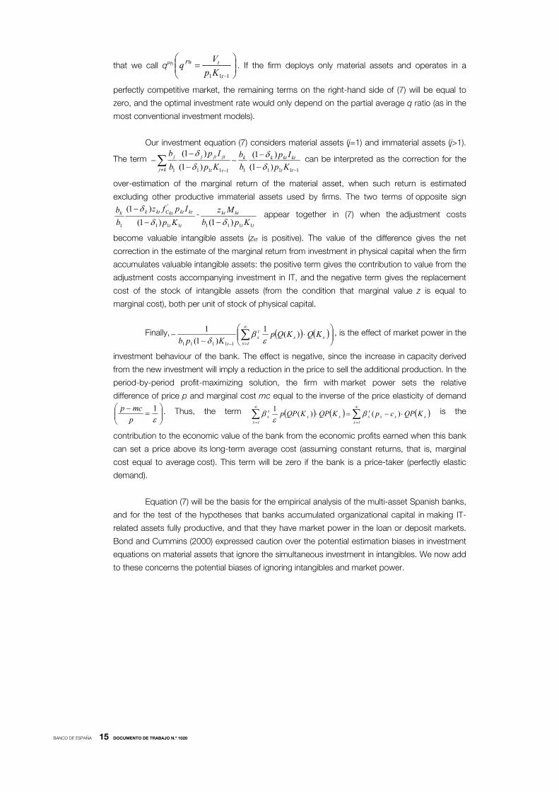
Equation (7) is an extension of the investment function derived by Bond and

Cummins (2000), to situations where: (i) firms have market power, and (ii) firms have adjustment

costs from IT investments that become valuable intangible assets. Suppose that asset 1 is the

material asset and the other assets are immaterial. The first term on the right-hand side of (7) is

the marginal return of material assets when this return is estimated with the partial average q,

6. Bond and Cummins (2000) derive their investment equation assuming a given proportion between tangible and intangible

stocks of capital assets. Under this assumption, their investment equation is the same as that derived in our paper.


that we call qPh

111 t

tPh

Kp

Vq . If the firm deploys only material assets and operates in a

perfectly competitive market, the remaining terms on the right-hand side of (7) will be equal to

zero, and the optimal investment rate would only depend on the partial average q ratio (as in the

most conventional investment models).

Our investment equation (7) considers material assets (j=1) and immaterial assets (j>1).

The term 1111111111 )1(

)1()1()1(

tt

ktktkk

kj tt

jtjtjj

Kp

Ip

b

b

Kp

Ip

b

b

can be interpreted as the correction for the

over-estimation of the marginal return of the material asset, when such return is estimated

excluding other productive immaterial assets used by firms. The two terms of opposite sign

tt

ktktktCktkk

Kp

Ipfz

b

b

111

'

1 )1()1(

-

tt

ktkt

Kpb

Mz

1111 )1( appear together in (7) when the adjustment costs

become valuable intangible assets (zkt is positive). The value of the difference gives the net

correction in the estimate of the marginal return from investment in physical capital when the firm

accumulates valuable intangible assets: the positive term gives the contribution to value from the

adjustment costs accompanying investment in IT, and the negative term gives the replacement

cost of the stock of intangible assets (from the condition that marginal value z is equal to

marginal cost), both per unit of stock of physical capital.

Finally,

s

tss

ts

t

KQKQpKpb

)(1)1(

1

11111

, is the effect of market power in the

investment behaviour of the bank. The effect is negative, since the increase in capacity derived

from the new investment will imply a reduction in the price to sell the additional production. In the

period-by-period profit-maximizing solution, the firm with market power sets the relative

difference of price p and marginal cost mc equal to the inverse of the price elasticity of demand

1

p

mcp . Thus, the term sts

sstss

tss

ts KQPcpKQPKQPp

)()(1

is the

contribution to the economic value of the bank from the economic profits earned when this bank

can set a price above its long-term average cost (assuming constant returns, that is, marginal

cost equal to average cost). This term will be zero if the bank is a price-taker (perfectly elastic

demand).

Equation (7) will be the basis for the empirical analysis of the multi-asset Spanish banks,

and for the test of the hypotheses that banks accumulated organizational capital in making IT-

related assets fully productive, and that they have market power in the loan or deposit markets.

Bond and Cummins (2000) expressed caution over the potential estimation biases in investment

equations on material assets that ignore the simultaneous investment in intangibles. We now add

to these concerns the potential biases of ignoring intangibles and market power.


3 Application to the Spanish banking industry

3.1 Database

Data on Spanish commercial and savings banks, from 1984 to 2003, are collected from

proprietary information provided by banks to the Banco de España (balance sheets, income

statements and complementary notes) at the non-consolidated level. The banks in the sample

represent 89.25% of the total banking assets in Spain in 2003 (the remainder are credit

cooperatives and branches of foreign banks). The number of banks in the sample changes over

time, from 160 in 1984 to 90 in 2003, because of mergers and acquisitions; the average number

of observations per bank is 13.23. The paper treats the banks that result from a merger as new

entities. We obtain estimates of the investment flow and capital stock of four main types of asset:

Physical (KPh), Information Technology (KIT), Advertising (KAD) and Financial (KFE). Physical capital

includes buildings (mainly branches) and durable assets.7 IT capital is set equal to the sum of the

assets reported in the balance sheet under the heading of information technology, plus the

capitalization of annual expenditures in IT reported in the income statement.8 Financial assets is

the counterpart, on the asset side of the balance sheet, of bank equity remaining after financing

the assets used in production and sales [Equity-(Physical + IT + Advertising)]. Regulatory

requirements for the minimum capital ratio for banks explain that this difference is positive under

normal conditions. Banks in the sample also report individual data on expenditures on training

workers, which is used to calculate the stock of intangible capital in the form of human capital

from training (KHK). The stocks of each of the assets are valued at current replacement cost, as

described in Appendix B.

In Spain, the banking industry has been unregulated for a long period of time. In line with

previous studies [Martín-Oliver and Salas-Fumás (2008)], we assume that Spanish commercial

and savings banks operate in a monopolistic competition framework with product differentiation.

As banks can have market power on loan markets, deposit markets, or both, we collect

individual bank data of the interest paid to deposits, ID, and of the gross profit margins in loans,

GLP (interest on loans minus opportunity cost of loans at the interbank interest rate) for the

estimation of the revenues in the investment equation. For loans, we use the gross margin, rather

than total interest payments, in order to avoid double-counting, since interest paid in deposits is

one component of the cost of loans.

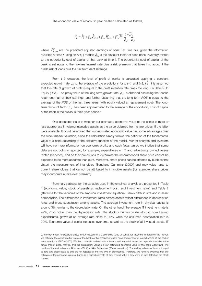
The (fundamental) economic value of the bank will be set equal to the present value of

the predicted future earnings, discounted at the cost of capital of the bank. We follow

the approach of Abel and Blanchard (1986) and forecast the future earnings of each bank

using an ARIMA econometric model. Earnings data are obtained from accounting earnings after

adjustment for differences in criteria between costs and investments:

cost treplacemen at assets immaterial and material

of onDepreciati Economic Estimated-onAmortizati Accounting

esExpenditur ITesExpenditur gAdvertisinEarnings AccountingEarnings Adjusted

7. Banks both rent and own their branches, so the replacement cost of physical assets has been calculated after having

homogenized all banks as if they owned all the branches they have. We are able to do this because we know the owned and

rented branches for each bank in the sample.

8. This paper does not explicitly distinguish between “hardware” and “software” when referring to IT capital and all IT assets

are named immaterial assets, because of data limitations. For example, we do not know the detailed components of IT

expenditures reported in the income statement of banks.


The economic value of a bank i in year t is then calculated as follows,

itit

itti

ti

ttiti

ttiti

titit PPPPV

1ˆˆˆˆ 3

,2,2,1,,

where t

stiP ,ˆ are the predicted adjusted earnings of bank i at time t+s, given the information

available at time t using an AR(2) model; ti, is the discount factor of each bank, inversely related

to the opportunity cost of capital of that bank at time t. The opportunity cost of capital of the

bank is set equal to the risk-free interest rate plus a risk premium that takes into account the

credit risk of loans plus the risk from debt leverage.

From t+3 onwards, the level of profit of banks is calculated applying a constant

expected growth rate i to the average of the predictions for t, t+1 and t+2,tiP . It is assumed

that this rate of growth of profit is equal to the profit retention rate times the long-run Return On

Equity (ROE). The proxy value of the long-term growth rate it is obtained assuming that banks

retain one half of their earnings, and further assuming that the long-term ROE is equal to the

average of the ROE of the last three years (with equity valued at replacement cost). The long-

term discount factor it has been approximated to the average of the opportunity cost of capital

of the bank in the previous three-year period.9

One debatable issue is whether our estimated economic value of the banks is more or

less appropriate in valuing intangible assets as the value obtained from share prices, if the latter

were available. It could be argued that our estimated economic value has some advantages over

the stock market valuation, since the calculation simply follows the definition of the fundamental

value of a bank according to the objective function of the model. Market analysts and investors

will have no more information on economic profits and cash flows tan do we (notice that some

data are not publicly reported; for example, expenditures on IT and advertising, owned versus

rented branches), and so their projections to determine the recommended share price cannot be

expected to be more accurate than ours. Moreover, share prices can be affected by bubbles that

distort the measurement of intangibles [Bond and Cummins (2000)] and may value rents to

current shareholders that cannot be attributed to intangible assets (for example, share prices

may incorporate a take-over premium).

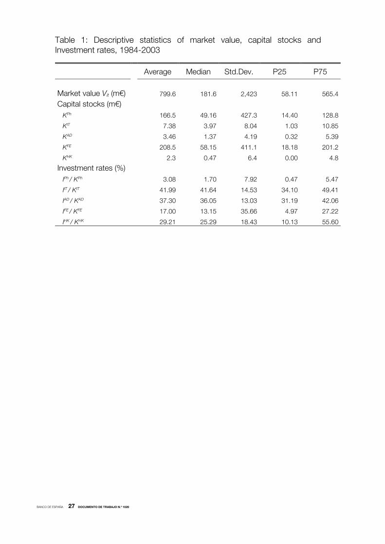
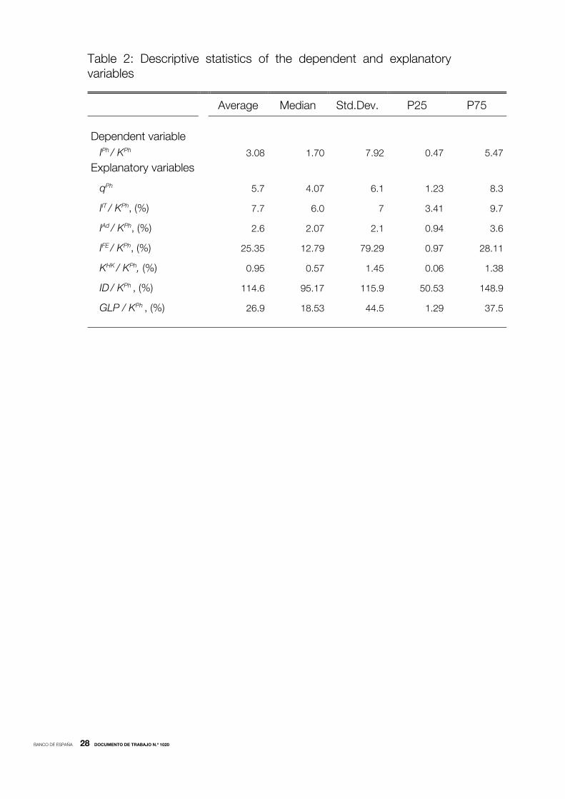
Summary statistics for the variables used in the empirical analysis are presented in Table

1 (economic value, stock of assets at replacement cost, and investment rates) and Table 2

(statistics for the variables of the empirical investment equation). Banks differ in size and in asset

composition. The differences in investment rates across assets reflect differences in depreciation

rates and cross-substitution among assets. The average investment rate in physical capital is

around 3%, similar to the depreciation rate. On the other hand, the average IT investment rate is

42%, 7 pp higher than the depreciation rate. The stock of human capital at cost, from training

expenditures, grows at an average rate close to 30%, while the assumed depreciation rate is

20%. Economic value of banks increases over time, as well as the stock of all invested assets. IT

9. In order to test for possible biases in our measure of the economic value of banks, for those banks listed on the market,

we estimate the actual market value of the bank as the product of share price and number of issued shares at the end of

each year (from 1987 to 2003). We then postulate and estimate a linear equation model, where the dependent variable is the

actual market price, Market, and the explanatory variable is our estimated economic value of the bank, Econvalue. The

results of the estimation are EconvalueMarket 09.183.79 (204 observations). The null hypothesis of intercept equal

to zero and slope equal to one are not rejected at the 5% level of significance. Therefore, we have no evidence that our

estimate of the economic value of banks is a biased estimate of their market value if they were, in fact, listed on the stock

market.


and advertising capital at constant prices increase during all the sample years, while physical

capital per worker increases only until 1996 and then begins a negative trend that persists until

2003. In 2003, the estimated stock of IT capital per worker at constant prices is 6.3 times what it

was in 1984, while Physical capital per worker in 2003 is 1.5 times what it was in 1984.

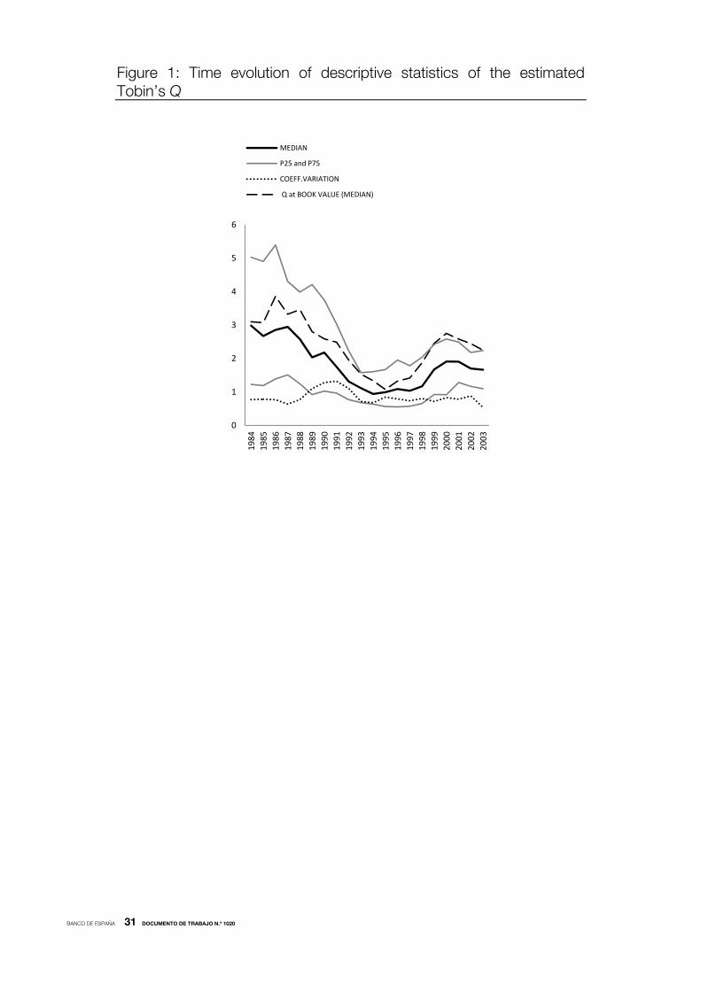
Figure 1 shows the time evolution of descriptive statistics for the q ratio, calculated as

the ratio between discounted adjusted cash flows and the assets of banks at replacement costs.

The median q ratio of the banks in the sample is close to 3 in 1984 and falls to 0.94 in 1994.

Since then, it rises again, but remains at values lower than 2. Increasing competition in the latter

part of the period (coinciding with the full liberalization of the banking sector, and with Spain

joining the Euro zone) squeezed economic profits. The coefficient of variation (standard deviation

divided by mean) also decrease over time, indicating convergence in the estimated q across

banks. For comparative purposes, Figure 1 also shows the median of the q ratio calculated with

raw accounting data (profits and book-reported assets). The median of the accounting-based q

ratio always overestimates the median of the q ratio with adjusted cash flows and assets at

replacement cost.

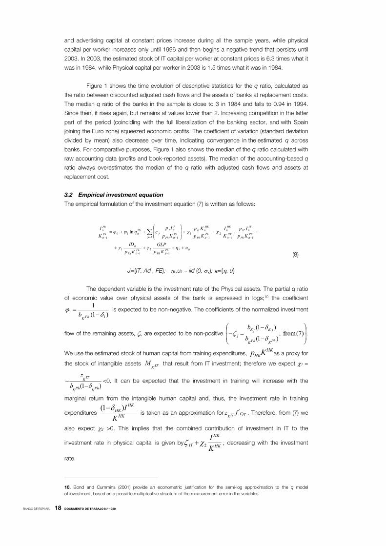
3.2 Empirical investment equation

The empirical formulation of the investment equation (7) is written as follows:

itiPhitPh

PhitPh

it

PhitPh

ITitIT

HKit

HKit

PhitPh

HKitH

JjPhitPh

jitj

jPhitPh

it

Phit

uKp

GLP

Kp

ID

Kp

Ip

K

I

Kp

Kp

Kp

Ipq

K

I

12

11

112

11

110

1

ln

J={IT, Ad , FE}; i ,uit ~ iid (0, ); ={, u}

(8)

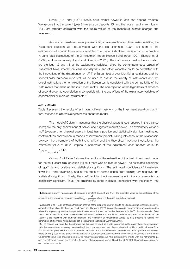
The dependent variable is the investment rate of the Physical assets. The partial q ratio

of economic value over physical assets of the bank is expressed in logs;10 the coefficient

)1(1

11

PhK

b is expected to be non-negative. The coefficients of the normalized investment

flow of the remaining assets, j, are expected to be non-positive

(7) from

)1(

)1( ,

PhKPhK

jKjK

j b

b

.

We use the estimated stock of human capital from training expenditures, HK

HKKp as a proxy for

the stock of intangible assets ITKM that result from IT investment; therefore we expect 1 =

)1( PhKPhK

ITK

b

z

<0. It can be expected that the investment in training will increase with the

marginal return from the intangible human capital and, thus, the investment rate in training

expenditures HK

HKHK

K

I)1( is taken as an approximation for ITCITK

fz '. Therefore, from (7) we

also expect 2 >0. This implies that the combined contribution of investment in IT to the

investment rate in physical capital is given byHK

HK

IT K

I2 , decreasing with the investment

rate.

10. Bond and Cummins (2001) provide an econometric justification for the semi-log approximation to the q model

of investment, based on a possible multiplicative structure of the measurement error in the variables.


Finally, 1 <0 and 2 <0 if banks have market power in loan and deposit markets.

We assume that the current (year t) interests on deposits, ID, and the gross margins from loans,

GLP, are strongly correlated with the future values of the respective interest charges and

revenues.11

As data on investment rates present a large cross-section and time-series variation, the

investment equation will be estimated with the first-differenced GMM estimator; all the

estimations will contain time-dummy variables. The use of first-differences is a common practice

in panel data estimations of the Q investment model [Hayashi and Inoue (1991); Blundell et al.

(1992); and, more recently, Bond and Cummins (2001)]. The instruments used in the estimation

are the lags t-2 and t-3 of the explanatory variables, since the contemporaneous values of

investment flows, interest on loans and deposits, and other variables, could be correlated with

the innovations of the disturbance term.12 The Sargan test of over-identifying restrictions and the

second-order autocorrelation test will be used to assess the validity of instruments and the

overall estimation: the non-rejection of the Sargan test is consistent with the compatibility of the

instruments that make up the instrument matrix. The non-rejection of the hypothesis of absence

of second-order autocorrelation is compatible with the use of lags of the explanatory variables of

second order or more as instruments.13

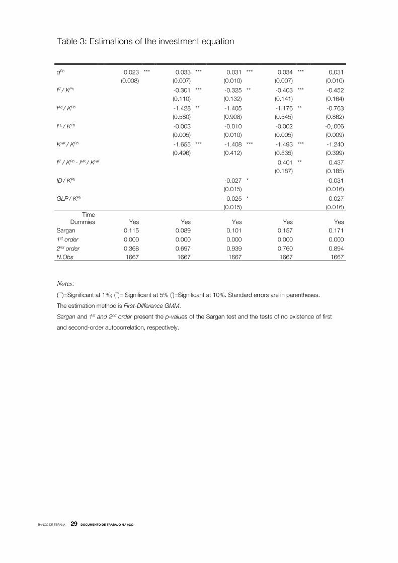
3.3 Results

Table 3 presents the results of estimating different versions of the investment equation that, in

turn, respond to alternative hypotheses about the model.

The model of Column 1 assumes that the physical assets (those reported in the balance

sheet) are the only capital input of banks, and it ignores market power. The explanatory variable

lnqPh (average q for physical assets in logs) has a positive and statistically significant estimated

coefficient, as conventional q models of investment predict. Taking into account the relationship

between the parameters of both the empirical and the theoretical investment equations, the

estimated value of 0.023 implies a parameter of the adjustment cost function equal to

8.44)1(

1

1

PhK

b .

Column 2 of Table 3 shows the results of the estimation of the basic investment model

for the multi-asset firm [equation (8)] as if there was no market power. The estimated coefficient

of Phqln is also positive and statistically significant. The estimated coefficients of investment

flows in IT and advertising, and of the stock of human capital from training, are negative and

statistically significant. Finally, the coefficient for the investment rate in financial assets is not

statistically significant. Thus, the empirical evidence indicates (consistent with the theory) that

11. Suppose a growth rate on sales of zero and a constant discount rate <1. The predicted value for the coefficient of the

revenues in the investment equation would be

)1(1

where is the price elasticity of demand.

12. Blundell et al. (1992) contains a thorough analysis of the proper number of lags to be used as suitable instruments in the

q investment equation. On the other hand, Bond and Cummins (2001) discuss the potential econometric problems in models

where the explanatory variable has persistent measurement errors, as can be the case with the Tobin’s q calculated from

stock market valuations, when these market valuations deviate from the firm’s fundamental value. Our estimates of the

Tobin’s q are obtained with earnings forecasts and estimates of fundamental values, so it is possible to identify the

parameters of the model with a suitable set of instruments [Bond and Cummins (2001)].

13. The second lag would be the minimum lag that can be used as a valid instrument in the case where the explanatory

variables are contemporaneously correlated with the disturbance term, and the equation is first-differenced to eliminate firm-

specific effects, provided that there is no serial correlation in the first-differenced residuals uit.. Although the measurement

errors of the q used in this paper are not related to persistent deviations between stock market valuations and the firm’s

fundamental value (see previous footnote), for robustness purposes we have estimated the model with the instruments qt-3

and qt-4 instead of qt-2 and qt-3, to control for potential measurement errors [Blundell et al. (1992)]. The results are similar for

each set of instruments.


banks face positive adjustment costs when they expand the stock of material, IT, and advertising

capital. However, the hypothesis that adjustment costs for financial assets are equal to zero

cannot be rejected, which suggests that Spanish banks were able to respond smoothly to the

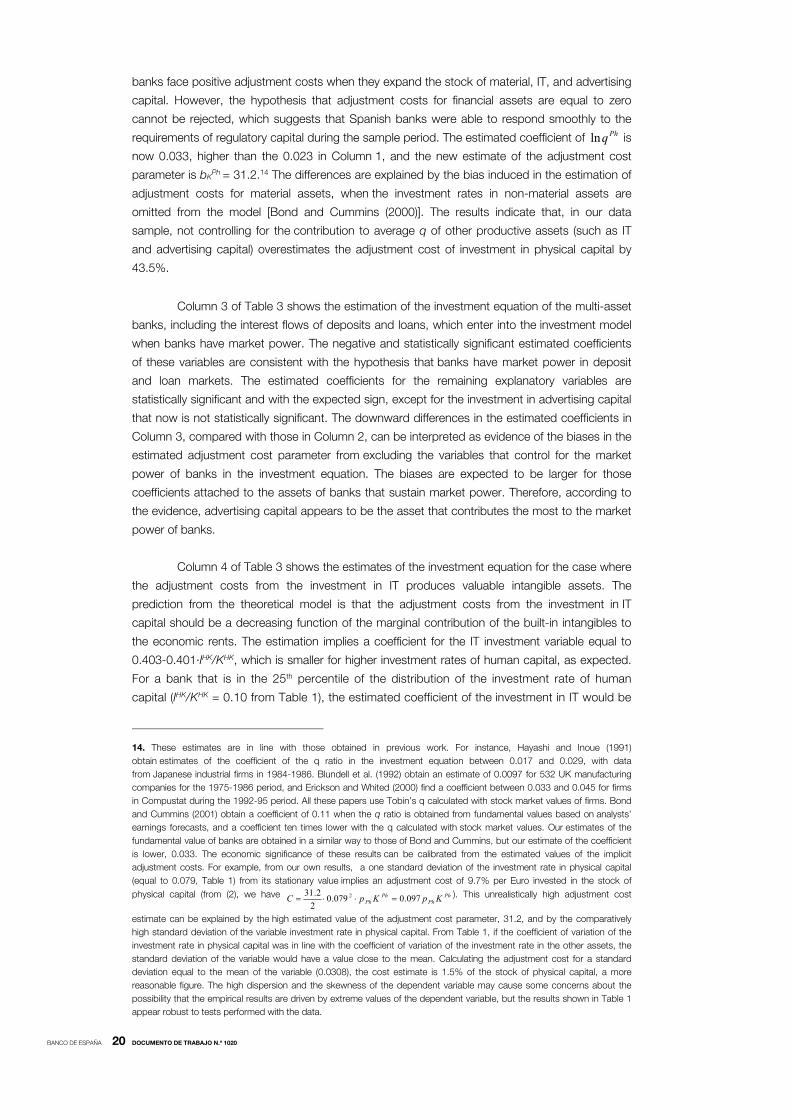
requirements of regulatory capital during the sample period. The estimated coefficient of Phqln is

now 0.033, higher than the 0.023 in Column 1, and the new estimate of the adjustment cost

parameter is bKPh

= 31.2.14 The differences are explained by the bias induced in the estimation of

adjustment costs for material assets, when the investment rates in non-material assets are

omitted from the model [Bond and Cummins (2000)]. The results indicate that, in our data

sample, not controlling for the contribution to average q of other productive assets (such as IT

and advertising capital) overestimates the adjustment cost of investment in physical capital by

43.5%.

Column 3 of Table 3 shows the estimation of the investment equation of the multi-asset

banks, including the interest flows of deposits and loans, which enter into the investment model

when banks have market power. The negative and statistically significant estimated coefficients

of these variables are consistent with the hypothesis that banks have market power in deposit

and loan markets. The estimated coefficients for the remaining explanatory variables are

statistically significant and with the expected sign, except for the investment in advertising capital

that now is not statistically significant. The downward differences in the estimated coefficients in

Column 3, compared with those in Column 2, can be interpreted as evidence of the biases in the

estimated adjustment cost parameter from excluding the variables that control for the market

power of banks in the investment equation. The biases are expected to be larger for those

coefficients attached to the assets of banks that sustain market power. Therefore, according to

the evidence, advertising capital appears to be the asset that contributes the most to the market

power of banks.

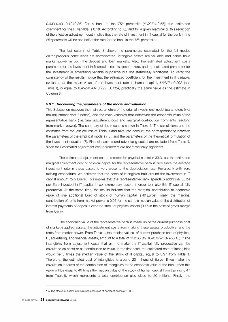
Column 4 of Table 3 shows the estimates of the investment equation for the case where

the adjustment costs from the investment in IT produces valuable intangible assets. The

prediction from the theoretical model is that the adjustment costs from the investment in IT

capital should be a decreasing function of the marginal contribution of the built-in intangibles to

the economic rents. The estimation implies a coefficient for the IT investment variable equal to

0.403-0.401·IHK/KHK, which is smaller for higher investment rates of human capital, as expected.

For a bank that is in the 25th percentile of the distribution of the investment rate of human

capital (IHK/KHK = 0.10 from Table 1), the estimated coefficient of the investment in IT would be

14. These estimates are in line with those obtained in previous work. For instance, Hayashi and Inoue (1991)

obtain estimates of the coefficient of the q ratio in the investment equation between 0.017 and 0.029, with data

from Japanese industrial firms in 1984-1986. Blundell et al. (1992) obtain an estimate of 0.0097 for 532 UK manufacturing

companies for the 1975-1986 period, and Erickson and Whited (2000) find a coefficient between 0.033 and 0.045 for firms

in Compustat during the 1992-95 period. All these papers use Tobin’s q calculated with stock market values of firms. Bond

and Cummins (2001) obtain a coefficient of 0.11 when the q ratio is obtained from fundamental values based on analysts’

earnings forecasts, and a coefficient ten times lower with the q calculated with stock market values. Our estimates of the

fundamental value of banks are obtained in a similar way to those of Bond and Cummins, but our estimate of the coefficient

is lower, 0.033. The economic significance of these results can be calibrated from the estimated values of the implicit

adjustment costs. For example, from our own results, a one standard deviation of the investment rate in physical capital

(equal to 0.079, Table 1) from its stationary value implies an adjustment cost of 9.7% per Euro invested in the stock of

physical capital (from (2), we have PhPh

PhPh KpKpC 097.0079.0

22.31 2 ). This unrealistically high adjustment cost

estimate can be explained by the high estimated value of the adjustment cost parameter, 31.2, and by the comparatively

high standard deviation of the variable investment rate in physical capital. From Table 1, if the coefficient of variation of the

investment rate in physical capital was in line with the coefficient of variation of the investment rate in the other assets, the

standard deviation of the variable would have a value close to the mean. Calculating the adjustment cost for a standard

deviation equal to the mean of the variable (0.0308), the cost estimate is 1.5% of the stock of physical capital, a more

reasonable figure. The high dispersion and the skewness of the dependent variable may cause some concerns about the

possibility that the empirical results are driven by extreme values of the dependent variable, but the results shown in Table 1

appear robust to tests performed with the data.


0.403-0.401·0.10=0.36. For a bank in the 75th percentile (IHK/KHK = 0.55), the estimated

coefficient for the IT variable is 0.18. According to (6), and for a given marginal q, this reduction

of the effective adjustment cost implies that the rate of investment in IT capital for the bank in the

25th percentile will be one half of the rate for the bank in the 75th percentile.

The last column of Table 3 shows the parameters estimated for the full model.

All the previous conclusions are corroborated: intangible assets are valuable and banks have

market power in both the deposit and loan markets. Also, the estimated adjustment costs

parameter for the investment in financial assets is close to zero, and the estimated parameter for

the investment in advertising variable is positive but not statistically significant. To verify the

consistency of the results, notice that the estimated coefficient for the investment in IT variable,

evaluated at the mean value of the investment rate in human capital, IHK/KHK = 0.292 (see

Table 1), is equal to 0.452-0.437·0.292 = 0.324, practically the same value as the estimate in

Column 3.

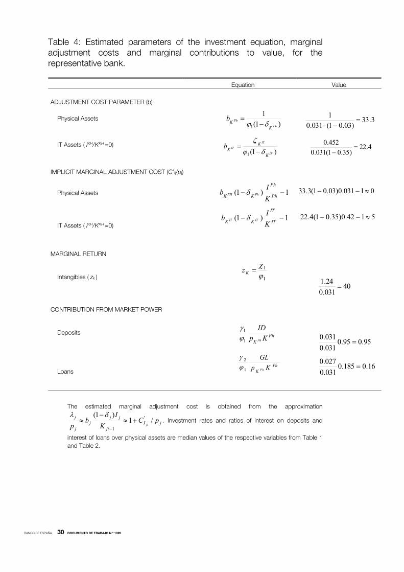
3.3.1 Recovering the parameters of the model and valuation

This Subsection recovers the main parameters of the original investment model (parameters bj of

the adjustment cost function), and the main variables that determine the economic value of the

representative bank (marginal adjustment cost and marginal contribution from rents resulting

from market power). The summary of the results is shown in Table 4. The calculations use the

estimates from the last column of Table 3 and take into account the correspondence between

the parameters of the empirical model in (8), and the parameters of the theoretical formulation of

the investment equation (7). Financial assets and advertising capital are excluded from Table 4,

since their estimated adjustment cost parameters are not statistically significant.

The estimated adjustment cost parameter for physical capital is 33.3, but the estimated

marginal adjustment cost of physical capital for the representative bank is zero since the average

investment rate in these assets is very close to the depreciation rate. For a bank with zero

training expenditure, we estimate that the costs of intangibles built around the investment in IT

capital amount to 5 Euros. This implies that the representative bank spends 5 additional Euros

per Euro invested in IT capital in complementary assets in order to make this IT capital fully

productive. At the same time, the results indicate that the marginal contribution to economic

value of one additional Euro of stock of human capital is 40 Euros. Finally, the marginal

contribution of rents from market power is 0.95 for the sample median value of the distribution of

interest payments of deposits over the stock of physical assets (0.16 in the case of gross margin

from loans).

The economic value of the representative bank is made up of the current purchase cost

of market-supplied assets, the adjustment costs from making these assets productive, and the

rents from market power. From Table 1, the median values of current purchase cost of physical,

IT, advertising, and financial assets, amount to a total of 112.65 (49.16+3.97+1.37+58.15).15 The

intangibles from adjustment costs that aim to make the IT capital fully productive can be

calculated as costs or as contribution to value. In the first case, the estimated cost of intangibles

would be 5 times the median value of the stock of IT capital, equal to 3.97 from Table 1.

Therefore, the estimated cost of intangibles is around 20 millions of Euros. If we make the

calculation in terms of the contribution of intangibles to the economic value of the bank, then this

value will be equal to 40 times the median value of the stock of human capital from training (0.47

from Table1), which represents a total contribution also close to 20 millions. Finally, the

15. The stocks of assets are in millions of Euros at constant prices of 1983.


contribution to market value of rents from market power are equal to the marginal contribution

times the median of the stock of physical capital (equal to 49.16 from Table 1). That is, a

contribution of 0.95·49.16=46.7 for deposits, and of 0.16·49.16 = 7.8 for loans, or a total

contribution of 54.5. With all these calculations, the estimated total economic value of this

representative bank would be 112.65+20+54.5 = 187.15, slightly above the median economic

value, from the sample data, of 181.6 (Table 1).


4 Conclusions and implications

Spanish banks invested heavily in IT during the period 1984 to 2003. On average, the stock of IT

capital per worker increased in this period from 2.9 to 21.1 thousands of constant Euros. This

paper provides evidence of the high investment in intangible assets that was carried out at the

same time as the investment in IT. According to our estimates, the average bank in the sample

has spent five additional Euros in intangible assets per Euro paid in market-purchased computers

and related assets. This implies that the replacement cost of the built-in intangibles represents

over 10% of the economic value of the bank, and around 40% of the replacement cost of

physical assets for the median values of the variables in the sample data. Expenditures in training

workers are part of these adjustment costs and the resulting human capital is part of the

intangible assets of the firm, though there will be other intangibles that are invisible to us. The

median replacement cost of the human capital from training is around 2.5% (0.47/20) of the

estimated replacement cost of intangibles from IT. Brynjolfsson, Hitt and Yang (2002) estimate

that, in their sample of non-financial firms, each dollar invested in IT required 12 additional dollars

of expenditure in intangibles. Compared to their findings, our sample of Spanish banks built a

lower stock of organization capital, though the estimation procedure is also different, and

comparisons of actual figures must be made with caution. We find no evidence of contribution to

the economic value of banks from adjustment costs attributed to investment in physical,

advertising, and financial assets. The finding that banks adjust the stock of financial assets

(equity minus material and immaterial assets at replacement cost) at no appreciable adjustment

cost suggests that banks did not face restrictions in meeting their economic capital requirements

under changing economic conditions.

We also find that rents from market power contribute to the economic value of the

representative bank: for the median values of the assets at replacement costs, the rents from

market power amount to around 28% of the economic value of the bank. The empirical evidence

suggests that advertising capital and, to a minor extent, physical capital and intangibles, can

explain part of the market power of banks. The rest would result from attributes specific to each

bank not captured by the explanatory variables of the model. Neither IT-related assets, nor

financial capital, appear to be determinants of banks’ economic rents. As a consequence, our

empirical evidence supports the view that investment in IT does not necessarily lead to a

competitive advantage for the bank.

This paper has several implications for research on the economic valuation of firms.

Assuming efficient capital markets, the market value of a listed firm is equal to the present value

of the expected future cash flows, discounted at the proper risk-adjusted discount factor

(fundamental value). The theory presented in this paper indicates that, if the assets invested by

the firm satisfy the value-maximization conditions, then the market value is expected to be equal

to the sum of the replacement cost of all the productive assets, plus the rents from market

power. The productive assets include material, immaterial, and intangibles, according to the

definitions for each class of assets used in this paper. If the rents from market power are zero,

and the replacement costs of the stock of material and immaterial assets are properly estimated,

the replacement cost of intangibles can be estimated by the difference between the market value

and the replacement costs of material and immaterial assets. However, if the firm has market

power (positive economic rents), this difference cannot be assimilated to the contribution of

intangibles to economic value (replacement costs plus attributed economic rents), since all

banks’ economic rents do not necessarily originate from intangible assets.


The investment equation of the multi-asset firm is directly related to the economic value

of the bank under rational, value-maximizing behaviour. The estimated adjustment costs from

this equation, if any, will be part of the economic value of the firm in addition to the market

purchase cost of the respective asset. The adjustment costs can then give an estimate of the

replacement cost of the built-in intangibles (if any), as we show in this paper. The lesson to be

drawn from our research is that one has to be careful of possible errors due to double-counting.

For example, expenses for training workers on how to use computers are part of the adjustment

costs attributed to investment in IT. If we calculate the cost of intangibles from the marginal

adjustment cost of investment in IT, as the model suggests, we do not need to add the direct

cost of intangibles, even if we could estimate them. In our analysis, the estimated stock of human

capital from training at replacement cost (0.47 for the median bank) should not be included in the

calculation of the replacement cost of all the productive assets, since it is already included in the

estimated replacement cost of all the intangibles associated with investments in IT. What our

calculations indicate is that the cost of human capital from training workers is only a minor part of

all the costs incurred in making the IT assets fully productive, but the actual nature of the

remaining intangibles is unknown to us at this point in our research.

Future research on the economic valuation and investment behaviour of the Spanish

banks would benefit of a more disaggregated database on IT capital, and more precise

estimates of the quality-adjusted price index of the IT capital. It would also be of interest to

compare the results obtained in this paper with those obtained with stock market valuations of

the equity of the banks. The number of listed banks in Spain is reduced and therefore it will be

difficult to replicate our analysis only with banks from this country, but the number of banks could

be expanded with listed banks from other countries.


REFERENCES

ABEL, A. B., and O. BLANCHARD (1986). “The present value of profits and cyclical movements in investment”,

Econometrica, 54, 2, pp. 249-273.

BASU, S., J. FERNAL, N. OULTON and S. SIRINIVASAN (2003). The case of missing productivity growth, or does IT explain

why productivity accelerated in the US but not in the UK?, NBER Macro Annual, also available as HIER Discussion Paper

2921.

BHARADWAJ, S., S. G. BHARADWAJ and B. R. KONSYNSKI (1999). “Information technology effects on firm performance

as measured by Tobin’s q”, Management Science, 45, 7, pp. 1008-1024.

BECALLI, E. (2007). “Does IT investment improve bank performance? Evidence from Europe?”, Journal of Banking and

Finance, 31, 7, pp. 2205-2230.

BLAIR, M., and S. WALLMAN (2001). Unseen Wealth: Report of the Brookings Task Force on Intangibles, Brookings

Institution Press, Washington DC.

BLUNDELL, R., S. BOND, M. DEVEREUX and F. SCHIANTARELLI (1992). “Investment and Tobin’s q: Evidence from

company panel data”, Journal of Econometrics, 51, pp. 233-258.

BOND, S., and J. CUMMINS (2000). “The stock market and investment in the new economy: Some tangible facts and

intangible fictions”, Brookings Papers, pp. 61-124.

― (2001). Noisy share prices and the Q model of Investment, IFS, Working Paper 01/22.

BOND, S., and C. MEGHIR (1994). “Dynamic investment models and the firm’s financial policy”, Review of Economic

Studies, 61, pp. 197-222.

BRESNAHAN, T., E. BRYNJOLFSSON and L. HITT (2002). “Information technology, workplace organization and the demand

for skilled labor: Firm level evidence”, Quarterly Journal of Economics, 117, pp. 339-376.

BRYNJOLFSSON, E., L. HITT and S. YANG (2002). “Intangible assets: Computers and organization capital”, Brookings

Papers on Economic Activity, pp. 137-181.

BRYNJOLFSSON, E., and S. YANG (1999). “The intangible costs and benefits of computer investment: Evidence from

financial markets”, Atlanta, Georgia: Proceedings of the International Conference on Information Systems.

BUIGES, P., A. JACQUEMIN and J. F. MARCHIPONT (eds.) (2000). Competitiveness and the Value of Intangible Assets,

Edward Elgar, Mass.

CARR, N. (2003). “IT Doesn’t Matter”, Harvard Business Review, 81, pp. 41-50.

COCKBURN, I., and Z. GRILICHES (1988). “Industry Effects and Appropriability Measures in the Stock Market’s Valuation of

R&D and Patents”, American Economic Review, 78, pp. 419-23.

CORRADO, C., J. HALTIWANGER and D. SICHEL (eds.) (2005). Measuring Capital in the New Economy, NBER Studies in

Income and Wealth, The University of Chicago Press: Chicago.

CORRADO C., C. HULTEN and D. SICHEL (2009). “Intangible Capital and Economic Growth”, Review of Income and

Wealth, 55, pp. 661-685.

CUMMINS, J. (2004). A new approach to the valuation of intangible capital, NBER Working Papers, No. 9924.

ERICKSON, T., and T. WHITED (2000). “Measurement Error and the Relationship between Investment and q”, Journal of

Political Economy, 108, pp. 1027-1057.

FUKAO, K., T. MIYAGAWA, K. MUKAI and Y. SHINODA (2009). “Intangible Investment in Japan: Measurement and

Contribution to Economic Growth”, Review of Income and Wealth, 55, pp. 717-736.

GRILICHES, Z. (1981). “Market value, R&D and patents, Economic Letters, 7, pp. 183-187.

HALL, B. (1993). “The Stock market valuation of R&D investment during the 1980s”, American Economic Review, 83,

pp. 259-264.

HALL, R. (2001). “The stock market and capital accumulation”, American Economic Review, 91, 6, pp. 1185-1202.

HAYASHI, F. (1982). “Tobin’s marginal q and average q: A neoclassical interpretation”, Econometrica, 50, pp. 213-224.

HAYASHI, F., and T. INOUE (1991). “The relation between firm growth and Q with multiple capital goods: Theory and

evidence from panel data on Japanese firms”, Econometrica, Vol. 59, 3, pp. 731-753.

HIRSCHEY, M., and J. WEYGANDT (1985). “Amortization policy for advertising and research and development

expenditures”, Journal of Accounting Research, Vol. 23, pp. 326-335.

HULTEN, CH., and X. HAO (2008). What is a company really worth? Intangible capital and the “market to book” value puzzle,

NBER Working Papers, No. 14548.

LEV, B. (2001). Intangibles: Management, measurement, and reporting, Brookings Institution Press, Washington, DC.

LEV, B., and S. RADHAKRISHNAN (2005). “The measurement of firm specific organizational capital”, in C. Corrado,

J. Haltiwanger and D. Sichel (eds.), Measuring capital in the new economy, Studies in Income and Wealth, Vol. 65,

The University of Chicago Press, Chicago, pp. 73-99.

LICHTENBERG, F. (1995). “The output contribution of computer equipment and personnel: a firm level analysis”, Journal of

Economics of Innovation and New Technology, 3, pp. 201-217.

MARRANO, M. G., J. HASKEL and G. WALLIS (2009). “What happened to the knowledge economy? ICT, Intangible

Investment, and Britain’s Productivity”, Review of Income and Wealth, 55, pp. 686-716.

MARTÍN-OLIVER, A., and V. SALAS-FUMÁS (2008). “The Output and Profit Contribution of Information Technology and

Advertising Investments in Banks”, Journal of Financial Intermediation, Vol. 17, pp. 229-255.

MARTÍN-OLIVER, A., V. SALAS-FUMÁS and J. SAURINA (2007). Measurement of Capital Stock and Input Services of

Spanish Banks”, Working Paper No. 0711, Banco de España.


MAS, M., and J. QUESADA (2005). Las nuevas tecnologías y el crecimiento económico en España, Fundación BBVA,

Madrid.

OLINER, S., D. SICHEL and K. STIROH (2007). “Explaining a Productive Decade”, Brookings Papers on Economic Activity,

1, pp. 81-152.

PRESCOTT, E., and M. VISSCHER (1980). “Organization capital”, Journal of Political Economy, 88, 3, pp. 446-461.

SCHIANTARELLY, F., and D. GEORGOUTSOS (1990). “Imperfect competition, Tobin’s q and investment: Evidence from

aggregate UK data”, European Economic Review, 34, pp. 1061-1078.

VILLALONGA, B. (2004). “Intangible resources, Tobin’s q and sustainability of performance differences”, Journal of

Economic Behaviour and Organization, 54, pp. 205-230.

WILDASIN, D. (1984). “The q Theory of Investment with Many Capital Goods”, The American Economic Review, 74, pp. 203-

210.


Table 1: Descriptive statistics of market value, capital stocks and Investment rates, 1984-2003

Average Median Std.Dev. P25 P75

Market value Vit (m€) 799.6 181.6 2,423 58.11 565.4

Capital stocks (m€)

KPh 166.5 49.16 427.3 14.40 128.8

KIT 7.38 3.97 8.04 1.03 10.85

KAD 3.46 1.37 4.19 0.32 5.39

KFE 208.5 58.15 411.1 18.18 201.2

KHK 2.3 0.47 6.4 0.00 4.8

Investment rates (%)

IPh / KPh 3.08 1.70 7.92 0.47 5.47

IIT / KIT 41.99 41.64 14.53 34.10 49.41

IAD / KAD 37.30 36.05 13.03 31.19 42.06

IFE / KFE 17.00 13.15 35.66 4.97 27.22

IHK / KHK 29.21 25.29 18.43 10.13 55.60


Table 2: Descriptive statistics of the dependent and explanatory variables

Average Median Std.Dev. P25 P75

Dependent variable

IPh / KPh 3.08 1.70 7.92 0.47 5.47

Explanatory variables

qPh 5.7 4.07 6.1 1.23 8.3

IIT / KPh, (%) 7.7 6.0 7 3.41 9.7

IAd / KPh, (%) 2.6 2.07 2.1 0.94 3.6

IFE / KPh, (%) 25.35 12.79 79.29 0.97 28.11

KHK / KPh, (%) 0.95 0.57 1.45 0.06 1.38

ID / KPh , (%) 114.6 95.17 115.9 50.53 148.9

GLP / KPh , (%) 26.9 18.53 44.5 1.29 37.5


Table 3: Estimations of the investment equation

qPh 0.023 *** 0.033 *** 0.031 *** 0.034 *** 0,031

(0.008) (0.007) (0.010) (0.007) (0.010)

IIT / KPh -0.301 *** -0.325 ** -0.403 *** -0.452

(0.110) (0.132) (0.141) (0.164)

IAd / KPh -1.428 ** -1.405 -1.176 ** -0.763

(0.580) (0.908) (0.545) (0.862)

IFE / KPh -0.003 -0.010 -0.002 -0,.006

(0.005) (0.010) (0.005) (0.009)

KHK / KPh -1.655 *** -1.408 *** -1.493 *** -1.240

(0.496) (0.412) (0.535) (0.399)

IIT / KPh ∙ IHK / KHK 0.401 ** 0.437

(0.187) (0.185)

ID / KPh -0.027 * -0.031

(0.015) (0.016)

GLP / KPh -0.025 * -0.027

(0.015) (0.016)

Time

Dummies Yes Yes Yes Yes Yes

Sargan 0.115 0.089 0.101 0.157 0.171

1st order 0.000 0.000 0.000 0.000 0.000

2nd order 0.368 0.697 0.939 0.760 0.894

N.Obs 1667 1667 1667 1667 1667

Notes:

(***)=Significant at 1%; (**)= Significant at 5% (*)=Significant at 10%. Standard errors are in parentheses.

The estimation method is First-Difference GMM.

Sargan and 1st and 2nd order present the p-values of the Sargan test and the tests of no existence of first

and second-order autocorrelation, respectively.


Table 4: Estimated parameters of the investment equation, marginal adjustment costs and marginal contributions to value, for the representative bank.

Equation Value

ADJUSTMENT COST PARAMETER (b)

Physical Assets

IT Assets ( IKH/KKH =0)

IMPLICIT MARGINAL ADJUSTMENT COST (C’Ij/pj)

Physical Assets

IT Assets ( IKH/KKH =0)

MARGINAL RETURN

Intangibles ( zk )

CONTRIBUTION FROM MARKET POWER

Deposits

Loans

The estimated marginal adjustment cost is obtained from the approximation

jIjt

jjj

j

j pCK

Ib

p jt/1

)1( '

1

. Investment rates and ratios of interest on deposits and

interest of loans over physical assets are median values of the respective variables from Table 1

and Table 2.

)1(1 IT

IT

IT

K

KK

b

4.22)35.01(031.0

452.0

1)1( Ph

Ph

KK K

Ib PhPH

1)1( IT

IT

KK K

Ib ITIT 5142.0)35.01(4.22

40031.024.1

1

1

Kz

PhK

Kp

ID

Ph1

1

95.095.0031.0031.0

PhK

Kp

GL

Ph1

2

16.0185.0031.0027.0

)1(1

1 Ph

Ph

KK

b

3.33)03.01(031.0

1

01031.0)03.01(3.33


Figure 1: Time evolution of descriptive statistics of the estimated Tobin’s Q

0

1

2

3

4

5

6

1984

1985

1986

1987

1988

1989

1990

1991

1992

1993

1994

1995

1996

1997

1998

1999

2000

2001

2002

2003

MEDIAN

P25 and P75

COEFF.VARIATION

Q at BOOK VALUE (MEDIAN)


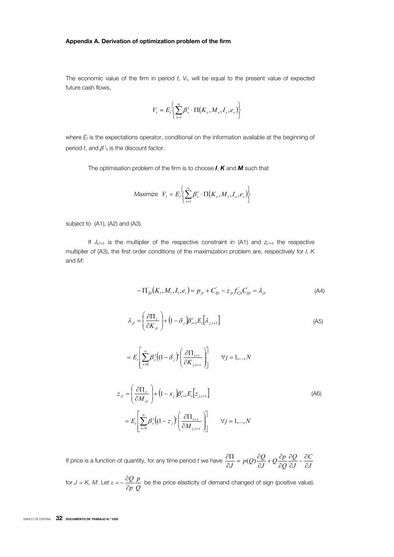
Appendix A. Derivation of optimization problem of the firm

The economic value of the firm in period t, Vt, will be equal to the present value of expected

future cash flows,

tsssss

tstt eIMKEV ,,,

where Et is the expectations operator, conditional on the information available at the beginning of

period t, and ts is the discount factor.

The optimisation problem of the firm is to choose I, K and M such that

Maximize

tsssss

tstt eIMKEV ,,,

subject to (A1), (A2) and (A3).

If j,t+s is the multiplier of the respective constraint in (A1) and zj,t+s the respective

multiplier of (A3), the first order conditions of the maximization problem are, respectively for I, K

and M:

jtIjtCjtjtIjtjtttttIjt CfzCpeIMK '''' ,,, (A4)

1,11

tjtttj

jt

tjt E

K (A5)

NjK

Es stj

stsj

tst ,...,11(

0 ,

1,11

tjtttj

jt

tjt zEx

Mz (A6)

NjM

zEs stj

stsj

tst ,...,11(

0 ,

If price is a function of quantity, for any time period t we have J

C

J

Q

Q

pQ

J

QQp

J

)(

for J = K, M. Let ε =Q

p

p

Q

be the price elasticity of demand changed of sign (positive value).


If Q=F(K,M) is linear homogeneous in K and M then,

.)(1)(j

j jjj

jj

j j K

CKQQpQQp

MM

KK

(A7)

Since C ( ) does not depend on M. Multiplying both sides of (A5) by Kj and adding and

subtracting jtjt I we have

jttjtttjjtjtjtjtjt

jt

tjtjt KEIIK

KK 1,11

Making use of (A4) and arranging the terms,

jttjtttjjt

jt

tjt

jt

tjtjtjt KEI

IK

KIK 1,11)(

Repeating the exercise with Mj in (A6),

jttjtttjjt

jt

tjtjt MzExM

MMz 1,11

Since the adjustment cost function tC ( ) in (A2) is also linear homogeneous in K and I,

summing over all j and taking into account (A7) we have,

jttjt

ttj j

j jttjtttjtttj j jtjtjtjtjt

MzEx

KEQQpMzIK

1,1

1,1

)1(

1)(1)(

Solving recursively,

tsts

tsttttts

tsjtj jtj jtjtjt VEQQpMzIK

)()(1)(

0

Finally, the economic value at the optimal solution is equal to,

sts

stsj jtjt

M

jjtjtjtt KQKQpMzIKV

)(1

(A8)

The investment model in the main text follows from (A8), (A4), (A5) and (A6) for the

particular case where only one asset, IT, generates intangible assets as a result of adjustment

costs.


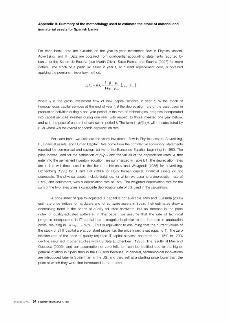
Appendix B. Summary of the methodology used to estimate the stock of material and

immaterial assets for Spanish banks

For each bank, data are available on the year-by-year investment flow in Physical assets,

Advertising, and IT. Data are obtained from confidential accounting statements reported by

banks to the Banco de España [see Martín-Oliver, Salas-Fumás and Saurina (2007) for more

details]. The stock of a particular asset in year t, at current replacement cost, is obtained

applying the permanent inventory method:

1111

1

ttt

ttttt Kp

p

pIpKp

where It is the gross investment flow of new capital services in year t; Kt the stock of

homogeneous capital services at the end of year t; the depreciation rate of the asset used in

production activities during a one-year period; the rate of technological progress incorporated

into capital services invested during one year, with respect to those invested one year before,

and pt is the price of one unit of services in period t. The term (1-)/(1+) will be substituted by

(1-) where is the overall economic depreciation rate.

For each bank, we estimate the yearly investment flow in Physical assets, Advertising,

IT, Financial assets, and Human Capital. Data come from the confidential accounting statements

reported by commercial and savings banks to the Banco de España, beginning in 1980. The

price indices used for the estimation of pt/pt-1 and the values of the depreciation rates, , that

enter into the permanent inventory equation, are summarized in Table B1. The depreciation rates

are in line with those used in the literature: Hirschey and Weygandt (1985) for advertising,

Litchenberg (1995) for IT and Hall (1993) for R&D/ human capital. Financial assets do not

depreciate. The physical assets include buildings, for which we assume a depreciation rate of

2.5%, and equipment, with a depreciation rate of 15%. The weighted depreciation rate for the

sum of the two rates gives a composite depreciation rate of 3% used in the calculation.

A price index of quality-adjusted IT capital is not available. Mas and Quesada (2005)

estimate price indices for hardware and for software assets in Spain; their estimates show a

decreasing trend in the prices of quality-adjusted hardware, but an increase in the price

index of quality-adjusted software. In this paper, we assume that the rate of technical

progress incorporated in IT capital has a magnitude similar to the increase in production

costs, resulting in 1/(1+ ) = pt/pt-1. This is equivalent to assuming that the current values of

the stock of all IT capital are at constant prices (i.e. the price index is set equal to 1). The zero

inflation rate of the price of quality-adjusted IT capital services contrasts the -15% to -20%

decline assumed in other studies with US data [Litchenberg (1995)]. The results of Mas and

Quesada (2005), and our assumption of zero inflation, can be justified due to the higher

general inflation in Spain than in the US, and because, in general, technological innovations

are introduced later in Spain than in the US, and they sell at a starting price lower than the

price at which they were first introduced in the market.


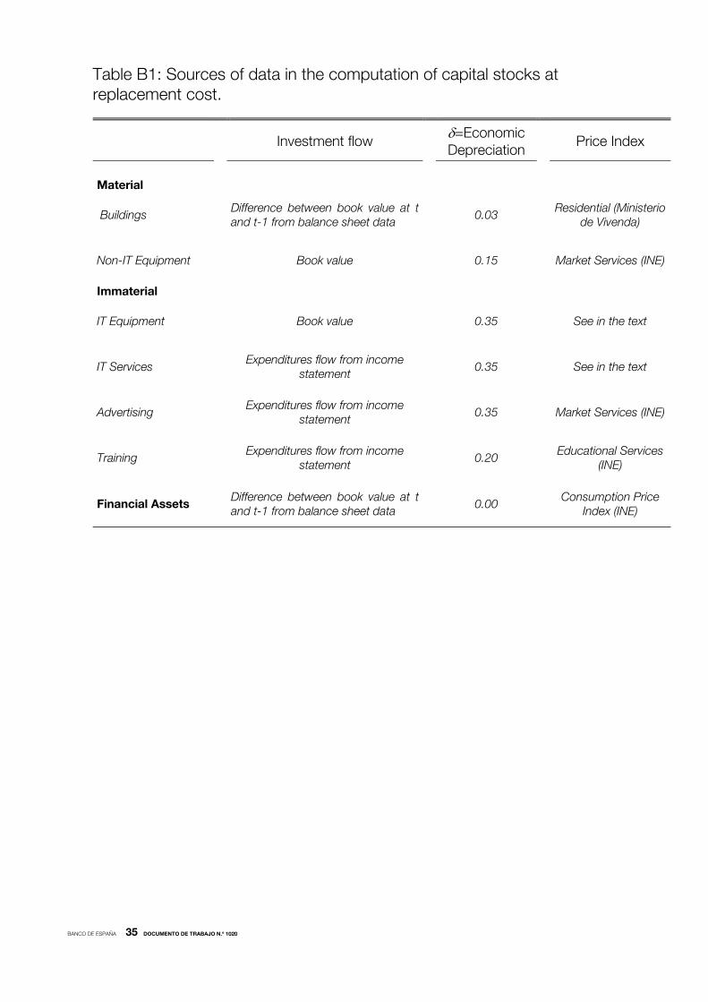
Table B1: Sources of data in the computation of capital stocks at replacement cost.

Investment flow

=Economic Depreciation Price Index

Material

Buildings

Difference between book value at t and t-1 from balance sheet data

0.03

Residential (Ministerio

de Vivenda)

Non-IT Equipment

Book value

0.15

Market Services (INE)

Immaterial

IT Equipment

Book value

0.35

See in the text

IT Services

Expenditures flow from income statement

0.35

See in the text

Advertising


0.35

Market Services (INE)

Training


0.20

Educational Services

(INE)

Financial Assets

Difference between book value at t and t-1 from balance sheet data

0.00

Consumption Price

Index (INE)

BANCO DE ESPAÑA PUBLICATIONS

WORKING PAPERS1

0901 PRAVEEN KUJAL AND JUAN RUIZ: International trade policy towards monopoly and oligopoly.

0902 CATIA BATISTA, AITOR LACUESTA AND PEDRO VICENTE: Micro evidence of the brain gain hypothesis: The case of Cape

Verde.

0903 MARGARITA RUBIO: Fixed and variable-rate mortgages, business cycles and monetary policy.

0904 MARIO IZQUIERDO, AITOR LACUESTA AND RAQUEL VEGAS: Assimilation of immigrants in Spain: A longitudinal analysis.

0905 ÁNGEL ESTRADA: The mark-ups in the Spanish economy: international comparison and recent evolution.

0906 RICARDO GIMENO AND JOSÉ MANUEL MARQUÉS: Extraction of financial market expectations about inflation and interest

rates from a liquid market.

0907 LAURA HOSPIDO: Job changes and individual-job specific wage dynamics.

0908 M.a DE LOS LLANOS MATEA AND JUAN S. MORA-SANGUINETTI: Developments in retail trade regulation in Spain and their

macroeconomic implications. (The original Spanish version has the same number.)

0909 JAVIER MENCÍA AND ENRIQUE SENTANA: Multivariate location-scale mixtures of normals and mean-variance-

skewness portfolio allocation.

0910 ALICIA GARCÍA-HERRERO, SERGIO GAVILÁ AND DANIEL SANTABÁRBARA: What explains the low profitability of

Chinese banks?

0911 JAVIER MENCÍA: Assessing the risk-return trade-off in loans portfolios.

0912 MAXIMO CAMACHO AND GABRIEL PEREZ-QUIROS: Ñ-STING: España Short Term Indicator of Growth.

0913 RAQUEL VEGAS, ISABEL ARGIMÓN, MARTA BOTELLA AND CLARA I. GONZÁLEZ: Retirement behaviour and

retirement incentives in Spain.

0914 FEDERICO CINGANO, MARCO LEONARDI, JULIÁN MESSINA AND GIOVANNI PICA: The effect of employment

protection legislation and financial market imperfections on investment: Evidence from a firm-level panel of EU

countries.

0915 JOSÉ MANUEL CAMPA AND IGNACIO HERNANDO: Cash, access to credit, and value creation in M&As.

0916 MARGARITA RUBIO: Housing market heterogeneity in a monetary union.

0917 MAXIMO CAMACHO, GABRIEL PEREZ-QUIROS AND HUGO RODRÍGUEZ MENDIZÁBAL: High-growth Recoveries,

Inventories and the Great Moderation.

0918 KAI CHRISTOFFEL, JAMES COSTAIN, GREGORY DE WALQUE, KEITH KUESTER, TOBIAS LINZERT, STEPHEN

MILLARD AND OLIVIER PIERRARD: Wage, inflation and employment dynamics with labour market matching.

0919 JESÚS VÁZQUEZ, RAMÓN MARÍA-DOLORES AND JUAN-MIGUEL LONDOÑO: On the informational role of term

structure in the U.S. monetary policy rule.

0920 PALOMA LÓPEZ-GARCÍA AND SERGIO PUENTE: What makes a high-growth firm? A probit analysis using Spanish

firm-level data.

0921 FABIO CANOVA, MATTEO CICCARELLI AND EVA ORTEGA: Do institutional changes affect business cycles?

Evidence from Europe.

0922 GALO NUÑO: Technology, convergence and business cycles.

0923 FRANCISCO DE CASTRO AND JOSÉ LUIS FERNÁNDEZ: The relationship between public and private saving in

Spain: does Ricardian equivalence hold?

0924 GONZALO FERNÁNDEZ-DE-CÓRDOBA, JAVIER J. PÉREZ AND JOSÉ L. TORRES: Public and private sector wages

interactions in a general equilibrium model.

0925 ÁNGEL ESTRADA AND JOSÉ MANUEL MONTERO: R&D investment and endogenous growth: a SVAR approach.

0926 JUANA ALEDO, FERNANDO GARCÍA-MARTÍNEZ AND JUAN M. MARÍN DIAZARAQUE: Firm-specific factors

influencing the selection of accounting options provided by the IFRS: Empirical evidence from Spanish market.

0927 JAVIER ANDRÉS, SAMUEL HURTADO, EVA ORTEGA AND CARLOS THOMAS: Spain in the euro: a general

equilibrium analysis.

0928 MAX GILLMAN AND ANTON NAKOV: Monetary effects on nominal oil prices.

0929

0930

JAVIER MENCÍA AND ENRIQUE SENTANA: Distributional tests in multivariate dynamic models with Normal and

Student t innovations.

JOAN PAREDES, PABLO BURRIEL, FRANCISCO DE CASTRO, DANIEL GARROTE, ESTHER GORDO AND JAVIER

J. PÉREZ: Fiscal policy shocks in the euro area and the US: an empirical assessment.

1. Previously published Working Papers are listed in the Banco de España publications catalogue.

0931 TERESA LEAL, DIEGO J. PEDREGAL AND JAVIER J. PÉREZ: Short-term monitoring of the Spanish Government

balance with mixed-frequencies models.

0932 ANTON NAKOV AND GALO NUÑO: Oilgopoly: a general equilibrium model of the oil-macroeconomy nexus.

0933 TERESA LEAL AND JAVIER J. PÉREZ: Análisis de las desviaciones presupuestarias aplicado al caso del presupuesto

del Estado.

0934 JAVIER J. PÉREZ AND A. JESÚS SÁNCHEZ: Is there a signalling role for public wages? Evidence for the euro area

based on macro data.

0935

1001

JOAN PAREDES, DIEGO J. PEDREGAL AND JAVIER J. PÉREZ: A quarterly fiscal database for the euro area based

on intra-annual fiscal information.

JAVIER ANDRÉS, ÓSCAR ARCE AND CARLOS THOMAS: Banking competition, collateral constraints and optimal

monetary policy.

1002 CRISTINA BARCELÓ AND ERNESTO VILLANUEVA: The response of household wealth to the risk of losing the job:

evidence from differences in firing costs.

1003

1004

ALEXANDER KARAIVANOV, SONIA RUANO, JESÚS SAURINA AND ROBERT TOWNSEND: No bank, one bank,

several banks: does it matter for investment?

GABRIEL PEREZ-QUIROS AND HUGO RODRÍGUEZ MENDIZÁBAL: Asymmetric standing facilities: an unexploited

monetary policy tool.

1005

1006

1007

1008

GABRIEL JIMÉNEZ, JOSE A. LOPEZ AND JESÚS SAURINA: How does competition impact bank

risk-taking?

GIUSEPPE BERTOLA, AURELIJUS DABUSINSKAS, MARCO HOEBERICHTS, MARIO IZQUIERDO, CLAUDIA

KWAPIL, JEREMI MONTORNÈS AND DANIEL RADOWSKI: Price, wage and employment response to shocks:

evidence from the WDN Survey.

JAVIER MENCÍA: Testing non-linear dependence in the Hedge Fund industry.

ALFREDO MARTÍN-OLIVER: From proximity to distant banking: Spanish banks in the EMU.

1009 GALO NUÑO: Optimal research and development expenditure: a general equilibrium approach.

1010

1011

1012

1013

1014

1015

LUIS J. ÁLVAREZ AND PABLO BURRIEL: Is a Calvo price setting model consistent with micro price data?

JENS HAGENDORFF, IGNACIO HERNANDO, MARÍA J. NIETO AND LARRY D. WALL: What do premiums paid for

bank M&As reflect? The case of the European Union.

DAVID DE ANTONIO LIEDO: General equilibrium restrictions for dynamic factor models.

JAMES COSTAIN, JUAN F. JIMENO AND CARLOS THOMAS: Employment fluctuations in a dual labor market.

LUIS M. VICEIRA Y RICARDO GIMENO: The euro as a reserve currency for global investors.

PALOMA LÓPEZ-GARCÍA AND JOSÉ MANUEL MONTERO: Understanding the Spanish business innovation gap:

The role of spillovers and firms' absorptive capacity.

1016

1017

1018

1019

1020

AITOR LACUESTA AND SERGIO PUENTE: El efecto del ciclo económico en las entradas y salidas de inmigrantes

en España.

REBEKKA CHRISTOPOULOU, JUAN F. JIMENO AND ANA LAMO: Changes in the wage structure in EU countries.

THOMAS BREUER, MARTIN JANDAČKA, JAVIER MENCÍA AND MARTIN SUMMER: A systematic approach to

multi-period stress testing of portfolio credit risk.

LUIS J. ÁLVAREZ AND PABLO BURRIEL: Micro-based estimates of heterogeneous pricing rules: The United States

vs. the euro area.

ALFREDO MARTÍN-OLIVER AND VICENTE SALAS-FUMÁS: I.T. investment and intangibles: Evidence from banks.

Unidad de Publicaciones Alcalá, 522; 28027 Madrid

Telephone +34 91 338 6363. Fax +34 91 998 6488 E-mail: [email protected]

www.bde.es

Documents

Documentos de Trabajo N.º 1020