Embed Size (px)
Citation preview

Documentation of the PLplot plotting software i
Documentation of the PLplot plotting software

Documentation of the PLplot plotting software ii
Copyright © 1994 Maurice J. LeBrun, Geoffrey FurnishCopyright © 2000-2005 Rafael LaboissièreCopyright © 2000-2016 Alan W. IrwinCopyright © 2001-2003 Joao CardosoCopyright © 2004 Andrew RoachCopyright © 2004-2013 Andrew RossCopyright © 2004-2016 Arjen MarkusCopyright © 2005 Thomas J. DuckCopyright © 2005-2010 Hazen BabcockCopyright © 2008 Werner SmekalCopyright © 2008-2016 Jerry BauckCopyright © 2009-2014 Hezekiah M. CartyCopyright © 2014-2015 Phil RosenbergCopyright © 2015 Jim Dishaw
Redistribution and use in source (XML DocBook) and “compiled” forms (HTML, PDF, PostScript, DVI, TeXinfo and so forth)with or without modification, are permitted provided that the following conditions are met:
1. Redistributions of source code (XMLDocBook) must retain the above copyright notice, this list of conditions and the followingdisclaimer as the first lines of this file unmodified.
2. Redistributions in compiled form (transformed to other DTDs, converted to HTML, PDF, PostScript, and other formats) mustreproduce the above copyright notice, this list of conditions and the following disclaimer in the documentation and/or othermaterials provided with the distribution.
Important: THIS DOCUMENTATION IS PROVIDED BY THE PLPLOT PROJECT “AS IS” AND ANY EXPRESS OR IM-PLIED WARRANTIES, INCLUDING, BUT NOT LIMITED TO, THE IMPLIED WARRANTIES OF MERCHANTABILITYAND FITNESS FOR A PARTICULAR PURPOSE ARE DISCLAIMED. IN NO EVENT SHALL THE PLPLOT PROJECTBE LIABLE FORANYDIRECT, INDIRECT, INCIDENTAL, SPECIAL, EXEMPLARY, OR CONSEQUENTIAL DAMAGES(INCLUDING, BUTNOTLIMITEDTO, PROCUREMENTOF SUBSTITUTEGOODSOR SERVICES; LOSSOFUSE, DATA,ORPROFITS; ORBUSINESS INTERRUPTION)HOWEVERCAUSEDANDONANYTHEORYOFLIABILITY,WHETHERIN CONTRACT, STRICT LIABILITY, OR TORT (INCLUDING NEGLIGENCE OR OTHERWISE) ARISING IN ANYWAYOUT OF THE USE OF THIS DOCUMENTATION, EVEN IF ADVISED OF THE POSSIBILITY OF SUCH DAMAGE.Release version: 5.15.0Release date: 2019-06-01

Documentation of the PLplot plotting software iii
COLLABORATORS
TITLE :
Documentation of the PLplot plotting soft-ware
ACTION NAME DATE SIGNATURE
WRITTEN BY Maurice J. LeBrunand GeoffreyFurnish
June 1, 2019
REVISION HISTORY
NUMBER DATE DESCRIPTION NAME

Documentation of the PLplot plotting software iv
Contents
I Introduction 1
1 Introduction 21.1 The PLplot plotting software . . . . . . . . . . . . . . . . . . . . . . . . . . . . . . . . . . . . . . . . . . . . . 21.2 Feature Summary . . . . . . . . . . . . . . . . . . . . . . . . . . . . . . . . . . . . . . . . . . . . . . . . . . . 3
1.2.1 Cross Platform . . . . . . . . . . . . . . . . . . . . . . . . . . . . . . . . . . . . . . . . . . . . . . . . 31.2.2 Language Bindings . . . . . . . . . . . . . . . . . . . . . . . . . . . . . . . . . . . . . . . . . . . . . . 31.2.3 Output File Formats . . . . . . . . . . . . . . . . . . . . . . . . . . . . . . . . . . . . . . . . . . . . . 31.2.4 Interactive Platforms . . . . . . . . . . . . . . . . . . . . . . . . . . . . . . . . . . . . . . . . . . . . . 4
1.3 Obtaining Access to PLplot . . . . . . . . . . . . . . . . . . . . . . . . . . . . . . . . . . . . . . . . . . . . . . 41.4 Configure, build, and install PLplot from source . . . . . . . . . . . . . . . . . . . . . . . . . . . . . . . . . . . 41.5 PLplot Copyright Licensing . . . . . . . . . . . . . . . . . . . . . . . . . . . . . . . . . . . . . . . . . . . . . . 51.6 Credits . . . . . . . . . . . . . . . . . . . . . . . . . . . . . . . . . . . . . . . . . . . . . . . . . . . . . . . . . 5
II Programming 6
2 Simple Use of PLplot 72.1 Plotting a Simple Graph . . . . . . . . . . . . . . . . . . . . . . . . . . . . . . . . . . . . . . . . . . . . . . . . 72.2 Initializing PLplot . . . . . . . . . . . . . . . . . . . . . . . . . . . . . . . . . . . . . . . . . . . . . . . . . . . 72.3 Defining Plot Scales and Axes . . . . . . . . . . . . . . . . . . . . . . . . . . . . . . . . . . . . . . . . . . . . . 82.4 Labelling the Graph . . . . . . . . . . . . . . . . . . . . . . . . . . . . . . . . . . . . . . . . . . . . . . . . . . 82.5 Drawing the Graph . . . . . . . . . . . . . . . . . . . . . . . . . . . . . . . . . . . . . . . . . . . . . . . . . . 8
2.5.1 Drawing Points . . . . . . . . . . . . . . . . . . . . . . . . . . . . . . . . . . . . . . . . . . . . . . . . 82.5.2 Drawing Lines or Curves . . . . . . . . . . . . . . . . . . . . . . . . . . . . . . . . . . . . . . . . . . . 82.5.3 Writing Text on a Graph . . . . . . . . . . . . . . . . . . . . . . . . . . . . . . . . . . . . . . . . . . . 92.5.4 Area Fills . . . . . . . . . . . . . . . . . . . . . . . . . . . . . . . . . . . . . . . . . . . . . . . . . . . 92.5.5 More Complex Graphs . . . . . . . . . . . . . . . . . . . . . . . . . . . . . . . . . . . . . . . . . . . . 9
2.6 Finishing Up . . . . . . . . . . . . . . . . . . . . . . . . . . . . . . . . . . . . . . . . . . . . . . . . . . . . . . 92.7 In Case of Error . . . . . . . . . . . . . . . . . . . . . . . . . . . . . . . . . . . . . . . . . . . . . . . . . . . . 9

Documentation of the PLplot plotting software v
3 Advanced Use of PLplot 103.1 Command Line Arguments . . . . . . . . . . . . . . . . . . . . . . . . . . . . . . . . . . . . . . . . . . . . . . 103.2 Devices . . . . . . . . . . . . . . . . . . . . . . . . . . . . . . . . . . . . . . . . . . . . . . . . . . . . . . . . 11
3.2.1 Driver Functions . . . . . . . . . . . . . . . . . . . . . . . . . . . . . . . . . . . . . . . . . . . . . . . 113.2.2 Family File Output . . . . . . . . . . . . . . . . . . . . . . . . . . . . . . . . . . . . . . . . . . . . . . 133.2.3 Specifying the Output Device . . . . . . . . . . . . . . . . . . . . . . . . . . . . . . . . . . . . . . . . . 14
3.3 Adding FreeType Library Support to Bitmap Drivers . . . . . . . . . . . . . . . . . . . . . . . . . . . . . . . . . 153.4 View Surfaces, (Sub-)Pages, Viewports and Windows . . . . . . . . . . . . . . . . . . . . . . . . . . . . . . . . 15
3.4.1 Defining the Viewport . . . . . . . . . . . . . . . . . . . . . . . . . . . . . . . . . . . . . . . . . . . . 153.4.2 Defining the Window . . . . . . . . . . . . . . . . . . . . . . . . . . . . . . . . . . . . . . . . . . . . . 163.4.3 Annotating the Viewport . . . . . . . . . . . . . . . . . . . . . . . . . . . . . . . . . . . . . . . . . . . 163.4.4 Setting up a Standard Window . . . . . . . . . . . . . . . . . . . . . . . . . . . . . . . . . . . . . . . . 17
3.5 Setting Line Attributes . . . . . . . . . . . . . . . . . . . . . . . . . . . . . . . . . . . . . . . . . . . . . . . . 173.6 Setting the Area Fill Pattern . . . . . . . . . . . . . . . . . . . . . . . . . . . . . . . . . . . . . . . . . . . . . . 173.7 Setting Color . . . . . . . . . . . . . . . . . . . . . . . . . . . . . . . . . . . . . . . . . . . . . . . . . . . . . 17
3.7.1 Color Map0 . . . . . . . . . . . . . . . . . . . . . . . . . . . . . . . . . . . . . . . . . . . . . . . . . . 183.7.2 Color Map1 . . . . . . . . . . . . . . . . . . . . . . . . . . . . . . . . . . . . . . . . . . . . . . . . . . 18
3.8 Setting Character Attributes . . . . . . . . . . . . . . . . . . . . . . . . . . . . . . . . . . . . . . . . . . . . . . 193.8.1 Hershey font system . . . . . . . . . . . . . . . . . . . . . . . . . . . . . . . . . . . . . . . . . . . . . . 193.8.2 Unicode font system . . . . . . . . . . . . . . . . . . . . . . . . . . . . . . . . . . . . . . . . . . . . . 20
3.8.2.1 The ps device driver . . . . . . . . . . . . . . . . . . . . . . . . . . . . . . . . . . . . . . . . 203.8.2.2 The gd and wingcc device drivers . . . . . . . . . . . . . . . . . . . . . . . . . . . . . . . . . 203.8.2.3 The svg device driver . . . . . . . . . . . . . . . . . . . . . . . . . . . . . . . . . . . . . . . . 213.8.2.4 The psttf, cairo, qt, and wxwidgets device drivers . . . . . . . . . . . . . . . . . . . . . . . . . 22
3.8.3 FCI . . . . . . . . . . . . . . . . . . . . . . . . . . . . . . . . . . . . . . . . . . . . . . . . . . . . . . 223.8.4 Escape sequences in text . . . . . . . . . . . . . . . . . . . . . . . . . . . . . . . . . . . . . . . . . . . 223.8.5 Character size adjustment . . . . . . . . . . . . . . . . . . . . . . . . . . . . . . . . . . . . . . . . . . . 24
3.9 Three-dimensional Plots . . . . . . . . . . . . . . . . . . . . . . . . . . . . . . . . . . . . . . . . . . . . . . . . 243.9.1 Surface Plots . . . . . . . . . . . . . . . . . . . . . . . . . . . . . . . . . . . . . . . . . . . . . . . . . 243.9.2 Contour Plots . . . . . . . . . . . . . . . . . . . . . . . . . . . . . . . . . . . . . . . . . . . . . . . . . 243.9.3 Shade plots . . . . . . . . . . . . . . . . . . . . . . . . . . . . . . . . . . . . . . . . . . . . . . . . . . 253.9.4 Image plots . . . . . . . . . . . . . . . . . . . . . . . . . . . . . . . . . . . . . . . . . . . . . . . . . . 253.9.5 Vector plots . . . . . . . . . . . . . . . . . . . . . . . . . . . . . . . . . . . . . . . . . . . . . . . . . . 25
3.10 Legends and color bars . . . . . . . . . . . . . . . . . . . . . . . . . . . . . . . . . . . . . . . . . . . . . . . . 25
4 Deploying programs that use PLplot 26

Documentation of the PLplot plotting software vi
5 Drivers which implement file devices 295.1 The qt driver . . . . . . . . . . . . . . . . . . . . . . . . . . . . . . . . . . . . . . . . . . . . . . . . . . . . . . 295.2 The cairo driver . . . . . . . . . . . . . . . . . . . . . . . . . . . . . . . . . . . . . . . . . . . . . . . . . . . . 295.3 The svg driver . . . . . . . . . . . . . . . . . . . . . . . . . . . . . . . . . . . . . . . . . . . . . . . . . . . . . 295.4 The ps driver . . . . . . . . . . . . . . . . . . . . . . . . . . . . . . . . . . . . . . . . . . . . . . . . . . . . . 295.5 The psttf driver . . . . . . . . . . . . . . . . . . . . . . . . . . . . . . . . . . . . . . . . . . . . . . . . . . . . 305.6 The pdf driver . . . . . . . . . . . . . . . . . . . . . . . . . . . . . . . . . . . . . . . . . . . . . . . . . . . . . 305.7 The gd driver . . . . . . . . . . . . . . . . . . . . . . . . . . . . . . . . . . . . . . . . . . . . . . . . . . . . . 305.8 The pstex driver . . . . . . . . . . . . . . . . . . . . . . . . . . . . . . . . . . . . . . . . . . . . . . . . . . . . 31
6 Drivers which implement interactive devices 326.1 The qt driver . . . . . . . . . . . . . . . . . . . . . . . . . . . . . . . . . . . . . . . . . . . . . . . . . . . . . . 326.2 The cairo driver . . . . . . . . . . . . . . . . . . . . . . . . . . . . . . . . . . . . . . . . . . . . . . . . . . . . 326.3 The xwin driver . . . . . . . . . . . . . . . . . . . . . . . . . . . . . . . . . . . . . . . . . . . . . . . . . . . . 326.4 The tk driver . . . . . . . . . . . . . . . . . . . . . . . . . . . . . . . . . . . . . . . . . . . . . . . . . . . . . . 336.5 The aqt driver . . . . . . . . . . . . . . . . . . . . . . . . . . . . . . . . . . . . . . . . . . . . . . . . . . . . . 336.6 The wxwidgets driver . . . . . . . . . . . . . . . . . . . . . . . . . . . . . . . . . . . . . . . . . . . . . . . . . 33
6.6.1 wxWidgets Driver Basics . . . . . . . . . . . . . . . . . . . . . . . . . . . . . . . . . . . . . . . . . . . 33
III Supported computer languages 34
7 C Language 35
8 Ada Language 408.1 Overview . . . . . . . . . . . . . . . . . . . . . . . . . . . . . . . . . . . . . . . . . . . . . . . . . . . . . . . 408.2 The Bindings . . . . . . . . . . . . . . . . . . . . . . . . . . . . . . . . . . . . . . . . . . . . . . . . . . . . . 40
8.2.1 Thin Binding . . . . . . . . . . . . . . . . . . . . . . . . . . . . . . . . . . . . . . . . . . . . . . . . . 408.2.2 The Thick Bindings . . . . . . . . . . . . . . . . . . . . . . . . . . . . . . . . . . . . . . . . . . . . . . 418.2.3 Standard Thick Binding Using Enhanced Names . . . . . . . . . . . . . . . . . . . . . . . . . . . . . . . 418.2.4 Thick Binding Using Traditional Names . . . . . . . . . . . . . . . . . . . . . . . . . . . . . . . . . . . 42
8.3 The Examples . . . . . . . . . . . . . . . . . . . . . . . . . . . . . . . . . . . . . . . . . . . . . . . . . . . . . 428.4 Obtaining the Software . . . . . . . . . . . . . . . . . . . . . . . . . . . . . . . . . . . . . . . . . . . . . . . . 42
8.4.1 Obtaining an Ada compiler . . . . . . . . . . . . . . . . . . . . . . . . . . . . . . . . . . . . . . . . . . 428.4.2 Download and install PLplot . . . . . . . . . . . . . . . . . . . . . . . . . . . . . . . . . . . . . . . . . 428.4.3 The Ada bindings to PLplot . . . . . . . . . . . . . . . . . . . . . . . . . . . . . . . . . . . . . . . . . . 42
8.5 How to use the Ada bindings . . . . . . . . . . . . . . . . . . . . . . . . . . . . . . . . . . . . . . . . . . . . . 438.5.1 Ada 95 versus Ada 2005 . . . . . . . . . . . . . . . . . . . . . . . . . . . . . . . . . . . . . . . . . . . 438.5.2 GNAT versus non-GNAT . . . . . . . . . . . . . . . . . . . . . . . . . . . . . . . . . . . . . . . . . . . 438.5.3 Sample command line project . . . . . . . . . . . . . . . . . . . . . . . . . . . . . . . . . . . . . . . . . 43
8.6 Unique Features of the Ada bindings . . . . . . . . . . . . . . . . . . . . . . . . . . . . . . . . . . . . . . . . . 44

Documentation of the PLplot plotting software vii
8.6.1 High-level features for simplified plotting . . . . . . . . . . . . . . . . . . . . . . . . . . . . . . . . . . . 448.6.1.1 Foreground-background control . . . . . . . . . . . . . . . . . . . . . . . . . . . . . . . . . . 44
8.6.1.1.1 Draw_On_Black, Draw_On_White . . . . . . . . . . . . . . . . . . . . . . . . . . . 448.6.1.2 Simple Plotters . . . . . . . . . . . . . . . . . . . . . . . . . . . . . . . . . . . . . . . . . . . 45
8.6.1.2.1 Multiplot_Pairs . . . . . . . . . . . . . . . . . . . . . . . . . . . . . . . . . . . . . 458.6.1.2.2 Simple_Plot . . . . . . . . . . . . . . . . . . . . . . . . . . . . . . . . . . . . . . . 458.6.1.2.3 Simple_Plot_Log_X . . . . . . . . . . . . . . . . . . . . . . . . . . . . . . . . . . . 458.6.1.2.4 Simple_Plot_Log_Y . . . . . . . . . . . . . . . . . . . . . . . . . . . . . . . . . . . 458.6.1.2.5 Simple_Plot_Log_XY . . . . . . . . . . . . . . . . . . . . . . . . . . . . . . . . . . 458.6.1.2.6 Simple_Plot_Pairs . . . . . . . . . . . . . . . . . . . . . . . . . . . . . . . . . . . . 458.6.1.2.7 Single_Plot . . . . . . . . . . . . . . . . . . . . . . . . . . . . . . . . . . . . . . . 458.6.1.2.8 Simple_Contour . . . . . . . . . . . . . . . . . . . . . . . . . . . . . . . . . . . . . 458.6.1.2.9 Simple_Mesh_3D . . . . . . . . . . . . . . . . . . . . . . . . . . . . . . . . . . . . 458.6.1.2.10 Simple_Surface_3D . . . . . . . . . . . . . . . . . . . . . . . . . . . . . . . . . . . 45
8.6.1.3 Simple color map manipulations . . . . . . . . . . . . . . . . . . . . . . . . . . . . . . . . . . 468.6.2 Integer Options Given Ada Names . . . . . . . . . . . . . . . . . . . . . . . . . . . . . . . . . . . . . . 468.6.3 One-offs . . . . . . . . . . . . . . . . . . . . . . . . . . . . . . . . . . . . . . . . . . . . . . . . . . . . 48
8.7 Parts That Retain a C Flavor . . . . . . . . . . . . . . . . . . . . . . . . . . . . . . . . . . . . . . . . . . . . . 488.7.1 Map-drawing . . . . . . . . . . . . . . . . . . . . . . . . . . . . . . . . . . . . . . . . . . . . . . . . . 48
8.8 Known Variances . . . . . . . . . . . . . . . . . . . . . . . . . . . . . . . . . . . . . . . . . . . . . . . . . . . 488.8.1 Documentation . . . . . . . . . . . . . . . . . . . . . . . . . . . . . . . . . . . . . . . . . . . . . . . . 488.8.2 API . . . . . . . . . . . . . . . . . . . . . . . . . . . . . . . . . . . . . . . . . . . . . . . . . . . . . . 49
8.9 Compilation notes . . . . . . . . . . . . . . . . . . . . . . . . . . . . . . . . . . . . . . . . . . . . . . . . . . . 498.9.1 Ada 95 Versus Ada 2005 . . . . . . . . . . . . . . . . . . . . . . . . . . . . . . . . . . . . . . . . . . . 498.9.2 GNAT Dependence . . . . . . . . . . . . . . . . . . . . . . . . . . . . . . . . . . . . . . . . . . . . . . 498.9.3 PLplot_Auxiliary . . . . . . . . . . . . . . . . . . . . . . . . . . . . . . . . . . . . . . . . . . . . . . . 49
8.10 Notes for Apple Macintosh OS X users . . . . . . . . . . . . . . . . . . . . . . . . . . . . . . . . . . . . . . . . 498.10.1 Using Apple’s Xcode IDE . . . . . . . . . . . . . . . . . . . . . . . . . . . . . . . . . . . . . . . . . . . 498.10.2 AquaTerm . . . . . . . . . . . . . . . . . . . . . . . . . . . . . . . . . . . . . . . . . . . . . . . . . . . 508.10.3 X11 . . . . . . . . . . . . . . . . . . . . . . . . . . . . . . . . . . . . . . . . . . . . . . . . . . . . . . 508.10.4 GNAT for OS X . . . . . . . . . . . . . . . . . . . . . . . . . . . . . . . . . . . . . . . . . . . . . . . 50
9 A C++ Interface for PLplot 519.1 Motivation for the C++ Interface . . . . . . . . . . . . . . . . . . . . . . . . . . . . . . . . . . . . . . . . . . . 519.2 Design of the PLplot C++ Interface . . . . . . . . . . . . . . . . . . . . . . . . . . . . . . . . . . . . . . . . . . 52
9.2.1 Stream/Object Identity . . . . . . . . . . . . . . . . . . . . . . . . . . . . . . . . . . . . . . . . . . . . 529.2.2 Namespace Management . . . . . . . . . . . . . . . . . . . . . . . . . . . . . . . . . . . . . . . . . . . 529.2.3 Abstraction of Data Layout . . . . . . . . . . . . . . . . . . . . . . . . . . . . . . . . . . . . . . . . . . 529.2.4 Callbacks and Shades . . . . . . . . . . . . . . . . . . . . . . . . . . . . . . . . . . . . . . . . . . . . . 539.2.5 Collapsing the API . . . . . . . . . . . . . . . . . . . . . . . . . . . . . . . . . . . . . . . . . . . . . . 53
9.3 Specializing the PLplot C++ Interface . . . . . . . . . . . . . . . . . . . . . . . . . . . . . . . . . . . . . . . . 539.4 Status of the C++ Interface . . . . . . . . . . . . . . . . . . . . . . . . . . . . . . . . . . . . . . . . . . . . . . 54

Documentation of the PLplot plotting software viii
10 Fortran Language 55
11 OCaml Language 6011.1 Overview . . . . . . . . . . . . . . . . . . . . . . . . . . . . . . . . . . . . . . . . . . . . . . . . . . . . . . . 6011.2 The Bindings . . . . . . . . . . . . . . . . . . . . . . . . . . . . . . . . . . . . . . . . . . . . . . . . . . . . . 60
11.2.1 Core Binding . . . . . . . . . . . . . . . . . . . . . . . . . . . . . . . . . . . . . . . . . . . . . . . . . 6011.2.2 OCaml-specific variations to the core PLplot API . . . . . . . . . . . . . . . . . . . . . . . . . . . . . . 6111.2.3 OCaml high level 2D plotting API . . . . . . . . . . . . . . . . . . . . . . . . . . . . . . . . . . . . . . 61
11.3 The Examples . . . . . . . . . . . . . . . . . . . . . . . . . . . . . . . . . . . . . . . . . . . . . . . . . . . . . 6111.4 Obtaining the Software . . . . . . . . . . . . . . . . . . . . . . . . . . . . . . . . . . . . . . . . . . . . . . . . 61
11.4.1 Obtaining the OCaml compiler . . . . . . . . . . . . . . . . . . . . . . . . . . . . . . . . . . . . . . . . 6111.5 How to use the OCaml bindings . . . . . . . . . . . . . . . . . . . . . . . . . . . . . . . . . . . . . . . . . . . . 61
11.5.1 How to setup findlib for use with the OCaml bindings . . . . . . . . . . . . . . . . . . . . . . . . . . . . 6111.5.2 Sample command line project (core API) . . . . . . . . . . . . . . . . . . . . . . . . . . . . . . . . . . . 6211.5.3 Sample command line project (OCaml-specific API) . . . . . . . . . . . . . . . . . . . . . . . . . . . . . 6211.5.4 Sample toplevel project . . . . . . . . . . . . . . . . . . . . . . . . . . . . . . . . . . . . . . . . . . . . 63
11.6 Known Issues . . . . . . . . . . . . . . . . . . . . . . . . . . . . . . . . . . . . . . . . . . . . . . . . . . . . . 63
12 Using PLplot from Python 64
13 Using PLplot from Tcl 6513.1 Motivation for the Tcl Interface to PLplot . . . . . . . . . . . . . . . . . . . . . . . . . . . . . . . . . . . . . . . 6513.2 Overview of the Tcl Language Binding . . . . . . . . . . . . . . . . . . . . . . . . . . . . . . . . . . . . . . . . 6613.3 The PLplot Tcl Matrix Extension . . . . . . . . . . . . . . . . . . . . . . . . . . . . . . . . . . . . . . . . . . . 68
13.3.1 Using Tcl Matrices from Tcl . . . . . . . . . . . . . . . . . . . . . . . . . . . . . . . . . . . . . . . . . 6813.3.2 Using Tcl Matrices from C . . . . . . . . . . . . . . . . . . . . . . . . . . . . . . . . . . . . . . . . . . 7213.3.3 Using Tcl Matrices from C++ . . . . . . . . . . . . . . . . . . . . . . . . . . . . . . . . . . . . . . . . . 7213.3.4 Extending the Tcl Matrix facility . . . . . . . . . . . . . . . . . . . . . . . . . . . . . . . . . . . . . . . 73
13.4 Contouring and Shading from Tcl . . . . . . . . . . . . . . . . . . . . . . . . . . . . . . . . . . . . . . . . . . . 7413.4.1 Drawing a Contour Plot from Tcl . . . . . . . . . . . . . . . . . . . . . . . . . . . . . . . . . . . . . . . 7413.4.2 Drawing a Shaded Plot from Tcl . . . . . . . . . . . . . . . . . . . . . . . . . . . . . . . . . . . . . . . 75
13.5 Understanding the Performance Characteristics of Tcl . . . . . . . . . . . . . . . . . . . . . . . . . . . . . . . . 75
14 Building an Extended WISH 7714.1 Introduction to Tcl . . . . . . . . . . . . . . . . . . . . . . . . . . . . . . . . . . . . . . . . . . . . . . . . . . . 77
14.1.1 Motivation for Tcl . . . . . . . . . . . . . . . . . . . . . . . . . . . . . . . . . . . . . . . . . . . . . . . 7714.1.2 Capabilities of Tcl . . . . . . . . . . . . . . . . . . . . . . . . . . . . . . . . . . . . . . . . . . . . . . . 7714.1.3 Acquiring Tcl . . . . . . . . . . . . . . . . . . . . . . . . . . . . . . . . . . . . . . . . . . . . . . . . . 78
14.2 Introduction to Tk . . . . . . . . . . . . . . . . . . . . . . . . . . . . . . . . . . . . . . . . . . . . . . . . . . . 7814.3 Introduction to [incr Tcl] . . . . . . . . . . . . . . . . . . . . . . . . . . . . . . . . . . . . . . . . . . . . . . . 79

Documentation of the PLplot plotting software ix
14.4 PLplot Extensions to Tcl . . . . . . . . . . . . . . . . . . . . . . . . . . . . . . . . . . . . . . . . . . . . . . . . 7914.5 Custom Extensions to Tcl . . . . . . . . . . . . . . . . . . . . . . . . . . . . . . . . . . . . . . . . . . . . . . . 80
14.5.1 WISH Construction . . . . . . . . . . . . . . . . . . . . . . . . . . . . . . . . . . . . . . . . . . . . . . 8014.5.2 WISH Linking . . . . . . . . . . . . . . . . . . . . . . . . . . . . . . . . . . . . . . . . . . . . . . . . 8114.5.3 WISH Programming . . . . . . . . . . . . . . . . . . . . . . . . . . . . . . . . . . . . . . . . . . . . . 81
15 Embedding Plots in Graphical User Interfaces 83
IV Reference 84
16 Bibliography 8516.1 References . . . . . . . . . . . . . . . . . . . . . . . . . . . . . . . . . . . . . . . . . . . . . . . . . . . . . . . 85
17 The Common API for PLplot 8617.1 pl_setcontlabelformat: Set format of numerical label for contours . . . . . . . . . . . . . . . . . . . . . 8717.2 pl_setcontlabelparam: Set parameters of contour labelling other than format of numerical label . . . . . . 8717.3 pladv: Advance the (sub-)page . . . . . . . . . . . . . . . . . . . . . . . . . . . . . . . . . . . . . . . . . . . 8817.4 plarc: Draw a circular or elliptical arc . . . . . . . . . . . . . . . . . . . . . . . . . . . . . . . . . . . . . . . 8817.5 plaxes: Draw a box with axes, etc. with arbitrary origin . . . . . . . . . . . . . . . . . . . . . . . . . . . . . 8817.6 plbin: Plot a histogram from binned data . . . . . . . . . . . . . . . . . . . . . . . . . . . . . . . . . . . . . 9017.7 plbop: Begin a new page . . . . . . . . . . . . . . . . . . . . . . . . . . . . . . . . . . . . . . . . . . . . . . 9017.8 plbox: Draw a box with axes, etc . . . . . . . . . . . . . . . . . . . . . . . . . . . . . . . . . . . . . . . . . . 9017.9 plbox3: Draw a box with axes, etc, in 3-d . . . . . . . . . . . . . . . . . . . . . . . . . . . . . . . . . . . . . 9217.10 plbtime: Calculate broken-down time from continuous time for the current stream . . . . . . . . . . . . . . . 9317.11 plcalc_world: Calculate world coordinates and corresponding window index from relative device coordinates 9417.12 plclear: Clear current (sub)page . . . . . . . . . . . . . . . . . . . . . . . . . . . . . . . . . . . . . . . . . 9417.13 plcol0: Set color, cmap0 . . . . . . . . . . . . . . . . . . . . . . . . . . . . . . . . . . . . . . . . . . . . . 9417.14 plcol1: Set color, cmap1 . . . . . . . . . . . . . . . . . . . . . . . . . . . . . . . . . . . . . . . . . . . . . 9517.15 plcolorbar: Plot color bar for image, shade or gradient plots . . . . . . . . . . . . . . . . . . . . . . . . . . 9517.16 plconfigtime: Configure the transformation between continuous and broken-down time for the current stream 9717.17 plcont: Contour plot . . . . . . . . . . . . . . . . . . . . . . . . . . . . . . . . . . . . . . . . . . . . . . . . 9817.18 plcpstrm: Copy state parameters from the reference stream to the current stream . . . . . . . . . . . . . . . . 9917.19 plctime: Calculate continuous time from broken-down time for the current stream . . . . . . . . . . . . . . . 9917.20 plend: End plotting session . . . . . . . . . . . . . . . . . . . . . . . . . . . . . . . . . . . . . . . . . . . . . 10017.21 plend1: End plotting session for current stream . . . . . . . . . . . . . . . . . . . . . . . . . . . . . . . . . . 10017.22 plenv0: Same as plenv but if in multiplot mode does not advance the subpage, instead clears it . . . . . . . . . . . 10017.23 plenv: Set up standard window and draw box . . . . . . . . . . . . . . . . . . . . . . . . . . . . . . . . . . . 10217.24 pleop: Eject current page . . . . . . . . . . . . . . . . . . . . . . . . . . . . . . . . . . . . . . . . . . . . . 10317.25 plerrx: Draw error bars in x direction . . . . . . . . . . . . . . . . . . . . . . . . . . . . . . . . . . . . . . . 10317.26 plerry: Draw error bars in the y direction . . . . . . . . . . . . . . . . . . . . . . . . . . . . . . . . . . . . . 103

Documentation of the PLplot plotting software x
17.27 plfamadv: Advance to the next family file on the next new page . . . . . . . . . . . . . . . . . . . . . . . . . 10417.28 plfill: Draw filled polygon . . . . . . . . . . . . . . . . . . . . . . . . . . . . . . . . . . . . . . . . . . . . 10417.29 plfill3: Draw filled polygon in 3D . . . . . . . . . . . . . . . . . . . . . . . . . . . . . . . . . . . . . . . . 10417.30 plflush: Flushes the output stream . . . . . . . . . . . . . . . . . . . . . . . . . . . . . . . . . . . . . . . . 10517.31 plfont: Set font . . . . . . . . . . . . . . . . . . . . . . . . . . . . . . . . . . . . . . . . . . . . . . . . . . 10517.32 plfontld: Load Hershey fonts . . . . . . . . . . . . . . . . . . . . . . . . . . . . . . . . . . . . . . . . . . 10517.33 plGetCursor: Wait for graphics input event and translate to world coordinates. . . . . . . . . . . . . . . . . . 10517.34 plgchr: Get character default height and current (scaled) height . . . . . . . . . . . . . . . . . . . . . . . . . 10617.35 plgcmap1_range: Get the cmap1 argument range for continuous color plots . . . . . . . . . . . . . . . . . . 10617.36 plgcol0: Returns 8-bit RGB values for given color index from cmap0 . . . . . . . . . . . . . . . . . . . . . . 10617.37 plgcol0a: Returns 8-bit RGB values and PLFLT alpha transparency value for given color index from cmap0 . . 10717.38 plgcolbg: Returns the background color (cmap0[0]) by 8-bit RGB value . . . . . . . . . . . . . . . . . . . . 10717.39 plgcolbga: Returns the background color (cmap0[0]) by 8-bit RGB value and PLFLT alpha transparency value 10717.40 plgcompression: Get the current device-compression setting . . . . . . . . . . . . . . . . . . . . . . . . . 10817.41 plgdev: Get the current device (keyword) name . . . . . . . . . . . . . . . . . . . . . . . . . . . . . . . . . . 10817.42 plgdidev: Get parameters that define current device-space window . . . . . . . . . . . . . . . . . . . . . . . 10817.43 plgdiori: Get plot orientation . . . . . . . . . . . . . . . . . . . . . . . . . . . . . . . . . . . . . . . . . . 10817.44 plgdiplt: Get parameters that define current plot-space window . . . . . . . . . . . . . . . . . . . . . . . . . 10917.45 plgdrawmode: Get drawing mode (depends on device support!) . . . . . . . . . . . . . . . . . . . . . . . . . 10917.46 plgfam: Get family file parameters . . . . . . . . . . . . . . . . . . . . . . . . . . . . . . . . . . . . . . . . . 10917.47 plgfci: Get FCI (font characterization integer) . . . . . . . . . . . . . . . . . . . . . . . . . . . . . . . . . . 10917.48 plgfnam: Get output file name . . . . . . . . . . . . . . . . . . . . . . . . . . . . . . . . . . . . . . . . . . . 11017.49 plgfont: Get family, style and weight of the current font . . . . . . . . . . . . . . . . . . . . . . . . . . . . . 11017.50 plglevel: Get the (current) run level . . . . . . . . . . . . . . . . . . . . . . . . . . . . . . . . . . . . . . . 11017.51 plgpage: Get page parameters . . . . . . . . . . . . . . . . . . . . . . . . . . . . . . . . . . . . . . . . . . . 11117.52 plgra: Switch to graphics screen . . . . . . . . . . . . . . . . . . . . . . . . . . . . . . . . . . . . . . . . . . 11117.53 plgradient: Draw linear gradient inside polygon . . . . . . . . . . . . . . . . . . . . . . . . . . . . . . . . 11117.54 plgriddata: Grid data from irregularly sampled data . . . . . . . . . . . . . . . . . . . . . . . . . . . . . . 11217.55 plgspa: Get current subpage parameters . . . . . . . . . . . . . . . . . . . . . . . . . . . . . . . . . . . . . . 11317.56 plgstrm: Get current stream number . . . . . . . . . . . . . . . . . . . . . . . . . . . . . . . . . . . . . . . 11317.57 plgver: Get the current library version number . . . . . . . . . . . . . . . . . . . . . . . . . . . . . . . . . . 11317.58 plgvpd: Get viewport limits in normalized device coordinates . . . . . . . . . . . . . . . . . . . . . . . . . . . 11317.59 plgvpw: Get viewport limits in world coordinates . . . . . . . . . . . . . . . . . . . . . . . . . . . . . . . . . 11417.60 plgxax: Get x axis parameters . . . . . . . . . . . . . . . . . . . . . . . . . . . . . . . . . . . . . . . . . . . 11417.61 plgyax: Get y axis parameters . . . . . . . . . . . . . . . . . . . . . . . . . . . . . . . . . . . . . . . . . . . 11417.62 plgzax: Get z axis parameters . . . . . . . . . . . . . . . . . . . . . . . . . . . . . . . . . . . . . . . . . . . 11517.63 plhist: Plot a histogram from unbinned data . . . . . . . . . . . . . . . . . . . . . . . . . . . . . . . . . . . 11517.64 plhlsrgb: Convert HLS color to RGB . . . . . . . . . . . . . . . . . . . . . . . . . . . . . . . . . . . . . . 11617.65 plimagefr: Plot a 2D matrix using cmap1 . . . . . . . . . . . . . . . . . . . . . . . . . . . . . . . . . . . . 116

Documentation of the PLplot plotting software xi
17.66 plimage: Plot a 2D matrix using cmap1 with automatic color adjustment . . . . . . . . . . . . . . . . . . . . . 11717.67 plinit: Initialize PLplot . . . . . . . . . . . . . . . . . . . . . . . . . . . . . . . . . . . . . . . . . . . . . . 11717.68 pljoin: Draw a line between two points . . . . . . . . . . . . . . . . . . . . . . . . . . . . . . . . . . . . . . 11817.69 pllab: Simple routine to write labels . . . . . . . . . . . . . . . . . . . . . . . . . . . . . . . . . . . . . . . . 11817.70 pllegend: Plot legend using discretely annotated filled boxes, lines, and/or lines of symbols . . . . . . . . . . . 11817.71 pllightsource: Sets the 3D position of the light source . . . . . . . . . . . . . . . . . . . . . . . . . . . . 12017.72 plline: Draw a line . . . . . . . . . . . . . . . . . . . . . . . . . . . . . . . . . . . . . . . . . . . . . . . . 12117.73 plline3: Draw a line in 3 space . . . . . . . . . . . . . . . . . . . . . . . . . . . . . . . . . . . . . . . . . . 12117.74 pllsty: Select line style . . . . . . . . . . . . . . . . . . . . . . . . . . . . . . . . . . . . . . . . . . . . . . 12117.75 plmap: Plot continental outline or shapefile data in world coordinates . . . . . . . . . . . . . . . . . . . . . . . 12117.76 plmapfill: Plot all or a subset of Shapefile data, filling the polygons . . . . . . . . . . . . . . . . . . . . . . . 12217.77 plmapline: Plot all or a subset of Shapefile data using lines in world coordinates . . . . . . . . . . . . . . . . 12317.78 plmapstring: Plot all or a subset of Shapefile data using strings or points in world coordinates . . . . . . . . . 12417.79 plmaptex: Draw text at points defined by Shapefile data in world coordinates . . . . . . . . . . . . . . . . . . 12517.80 plmeridians: Plot latitude and longitude lines . . . . . . . . . . . . . . . . . . . . . . . . . . . . . . . . . . 12517.81 plmesh: Plot surface mesh . . . . . . . . . . . . . . . . . . . . . . . . . . . . . . . . . . . . . . . . . . . . . 12617.82 plmeshc: Magnitude colored plot surface mesh with contour . . . . . . . . . . . . . . . . . . . . . . . . . . . 12617.83 plmkstrm: Creates a new stream and makes it the default . . . . . . . . . . . . . . . . . . . . . . . . . . . . . 12717.84 plmtex: Write text relative to viewport boundaries . . . . . . . . . . . . . . . . . . . . . . . . . . . . . . . . 12717.85 plmtex3: Write text relative to viewport boundaries in 3D plots . . . . . . . . . . . . . . . . . . . . . . . . . . 12817.86 plot3d: Plot 3-d surface plot . . . . . . . . . . . . . . . . . . . . . . . . . . . . . . . . . . . . . . . . . . . . 12917.87 plot3dc: Magnitude colored plot surface with contour . . . . . . . . . . . . . . . . . . . . . . . . . . . . . . 12917.88 plot3dcl: Magnitude colored plot surface with contour for z[x][y] with y index limits . . . . . . . . . . . . . . 13017.89 plparseopts: Parse command-line arguments . . . . . . . . . . . . . . . . . . . . . . . . . . . . . . . . . . 13117.90 plpat: Set area line fill pattern . . . . . . . . . . . . . . . . . . . . . . . . . . . . . . . . . . . . . . . . . . . 13217.91 plpath: Draw a line between two points, accounting for coordinate transforms . . . . . . . . . . . . . . . . . . 13217.92 plpoin: Plot a glyph at the specified points . . . . . . . . . . . . . . . . . . . . . . . . . . . . . . . . . . . . 13217.93 plpoin3: Plot a glyph at the specified 3D points . . . . . . . . . . . . . . . . . . . . . . . . . . . . . . . . . . 13317.94 plpoly3: Draw a polygon in 3 space . . . . . . . . . . . . . . . . . . . . . . . . . . . . . . . . . . . . . . . . 13317.95 plprec: Set precision in numeric labels . . . . . . . . . . . . . . . . . . . . . . . . . . . . . . . . . . . . . . 13417.96 plpsty: Select area fill pattern . . . . . . . . . . . . . . . . . . . . . . . . . . . . . . . . . . . . . . . . . . . 13417.97 plptex: Write text inside the viewport . . . . . . . . . . . . . . . . . . . . . . . . . . . . . . . . . . . . . . . 13417.98 plptex3: Write text inside the viewport of a 3D plot . . . . . . . . . . . . . . . . . . . . . . . . . . . . . . . 13517.99 plrandd: Random number generator returning a real random number in the range [0,1] . . . . . . . . . . . . . 13617.100plreplot: Replays contents of plot buffer to current device/file . . . . . . . . . . . . . . . . . . . . . . . . . 13617.101plrgbhls: Convert RGB color to HLS . . . . . . . . . . . . . . . . . . . . . . . . . . . . . . . . . . . . . . 13617.102plschr: Set character size . . . . . . . . . . . . . . . . . . . . . . . . . . . . . . . . . . . . . . . . . . . . . 13717.103plscmap0: Set cmap0 colors by 8-bit RGB values . . . . . . . . . . . . . . . . . . . . . . . . . . . . . . . . . 13717.104plscmap0a: Set cmap0 colors by 8-bit RGB values and PLFLT alpha transparency value . . . . . . . . . . . . 137

Documentation of the PLplot plotting software xii
17.105plscmap0n: Set number of colors in cmap0 . . . . . . . . . . . . . . . . . . . . . . . . . . . . . . . . . . . . 13817.106plscmap1_range: Set the cmap1 argument range for continuous color plots . . . . . . . . . . . . . . . . . . 13817.107plscmap1: Set opaque RGB cmap1 colors values . . . . . . . . . . . . . . . . . . . . . . . . . . . . . . . . . 13817.108plscmap1a: Set semitransparent cmap1 RGBA colors. . . . . . . . . . . . . . . . . . . . . . . . . . . . . . . 13917.109plscmap1l: Set cmap1 colors using a piece-wise linear relationship . . . . . . . . . . . . . . . . . . . . . . . 13917.110plscmap1la: Set cmap1 colors and alpha transparency using a piece-wise linear relationship . . . . . . . . . . 14017.111plscmap1n: Set number of colors in cmap1 . . . . . . . . . . . . . . . . . . . . . . . . . . . . . . . . . . . . 14117.112plscol0: Set 8-bit RGB values for given cmap0 color index . . . . . . . . . . . . . . . . . . . . . . . . . . . 14117.113plscol0a: Set 8-bit RGB values and PLFLT alpha transparency value for given cmap0 color index . . . . . . . 14117.114plscolbg: Set the background color by 8-bit RGB value . . . . . . . . . . . . . . . . . . . . . . . . . . . . . 14217.115plscolbga: Set the background color by 8-bit RGB value and PLFLT alpha transparency value. . . . . . . . . 14217.116plscolor: Used to globally turn color output on/off . . . . . . . . . . . . . . . . . . . . . . . . . . . . . . . 14217.117plscompression: Set device-compression level . . . . . . . . . . . . . . . . . . . . . . . . . . . . . . . . . 14317.118plsdev: Set the device (keyword) name . . . . . . . . . . . . . . . . . . . . . . . . . . . . . . . . . . . . . . 14317.119plsdidev: Set parameters that define current device-space window . . . . . . . . . . . . . . . . . . . . . . . . 14317.120plsdimap: Set up transformation from metafile coordinates . . . . . . . . . . . . . . . . . . . . . . . . . . . . 14417.121plsdiori: Set plot orientation . . . . . . . . . . . . . . . . . . . . . . . . . . . . . . . . . . . . . . . . . . . 14417.122plsdiplt: Set parameters that define current plot-space window . . . . . . . . . . . . . . . . . . . . . . . . . 14417.123plsdiplz: Set parameters incrementally (zoom mode) that define current plot-space window . . . . . . . . . . 14517.124plsdrawmode: Set drawing mode (depends on device support!) . . . . . . . . . . . . . . . . . . . . . . . . . 14517.125plseed: Set seed for internal random number generator. . . . . . . . . . . . . . . . . . . . . . . . . . . . . . 14517.126plsesc: Set the escape character for text strings . . . . . . . . . . . . . . . . . . . . . . . . . . . . . . . . . . 14517.127plsetopt: Set any command-line option . . . . . . . . . . . . . . . . . . . . . . . . . . . . . . . . . . . . . 14617.128plsfam: Set family file parameters . . . . . . . . . . . . . . . . . . . . . . . . . . . . . . . . . . . . . . . . . 14617.129plsfci: Set FCI (font characterization integer) . . . . . . . . . . . . . . . . . . . . . . . . . . . . . . . . . . 14717.130plsfnam: Set output file name . . . . . . . . . . . . . . . . . . . . . . . . . . . . . . . . . . . . . . . . . . . 14717.131plsfont: Set family, style and weight of the current font . . . . . . . . . . . . . . . . . . . . . . . . . . . . . 14717.132plshades: Shade regions on the basis of value . . . . . . . . . . . . . . . . . . . . . . . . . . . . . . . . . . 14817.133plshade: Shade individual region on the basis of value . . . . . . . . . . . . . . . . . . . . . . . . . . . . . . 14917.134plslabelfunc: Assign a function to use for generating custom axis labels . . . . . . . . . . . . . . . . . . . 15017.135plsmaj: Set length of major ticks . . . . . . . . . . . . . . . . . . . . . . . . . . . . . . . . . . . . . . . . . 15117.136plsmem: Set the memory area to be plotted (RGB) . . . . . . . . . . . . . . . . . . . . . . . . . . . . . . . . . 15117.137plsmema: Set the memory area to be plotted (RGBA) . . . . . . . . . . . . . . . . . . . . . . . . . . . . . . . 15117.138plsmin: Set length of minor ticks . . . . . . . . . . . . . . . . . . . . . . . . . . . . . . . . . . . . . . . . . 15217.139plsori: Set orientation . . . . . . . . . . . . . . . . . . . . . . . . . . . . . . . . . . . . . . . . . . . . . . . 15217.140plspage: Set page parameters . . . . . . . . . . . . . . . . . . . . . . . . . . . . . . . . . . . . . . . . . . . 15217.141plspal0: Set the cmap0 palette using the specified cmap0*.pal format file . . . . . . . . . . . . . . . . . . 15317.142plspal1: Set the cmap1 palette using the specified cmap1*.pal format file . . . . . . . . . . . . . . . . . . 15317.143plspause: Set the pause (on end-of-page) status . . . . . . . . . . . . . . . . . . . . . . . . . . . . . . . . . 153

Documentation of the PLplot plotting software xiii
17.144plsstrm: Set current output stream . . . . . . . . . . . . . . . . . . . . . . . . . . . . . . . . . . . . . . . . 15317.145plssub: Set the number of subpages in x and y . . . . . . . . . . . . . . . . . . . . . . . . . . . . . . . . . . 15417.146plssym: Set symbol size . . . . . . . . . . . . . . . . . . . . . . . . . . . . . . . . . . . . . . . . . . . . . . 15417.147plstar: Initialization . . . . . . . . . . . . . . . . . . . . . . . . . . . . . . . . . . . . . . . . . . . . . . . . 15417.148plstart: Initialization . . . . . . . . . . . . . . . . . . . . . . . . . . . . . . . . . . . . . . . . . . . . . . . 15417.149plstransform: Set a global coordinate transform function . . . . . . . . . . . . . . . . . . . . . . . . . . . 15517.150plstring: Plot a glyph at the specified points . . . . . . . . . . . . . . . . . . . . . . . . . . . . . . . . . . . 15517.151plstring3: Plot a glyph at the specified 3D points . . . . . . . . . . . . . . . . . . . . . . . . . . . . . . . . 15617.152plstripa: Add a point to a strip chart . . . . . . . . . . . . . . . . . . . . . . . . . . . . . . . . . . . . . . 15617.153plstripc: Create a 4-pen strip chart . . . . . . . . . . . . . . . . . . . . . . . . . . . . . . . . . . . . . . . 15617.154plstripd: Deletes and releases memory used by a strip chart . . . . . . . . . . . . . . . . . . . . . . . . . . . 15717.155plstyl: Set line style . . . . . . . . . . . . . . . . . . . . . . . . . . . . . . . . . . . . . . . . . . . . . . . . 15817.156plsurf3d: Plot shaded 3-d surface plot . . . . . . . . . . . . . . . . . . . . . . . . . . . . . . . . . . . . . . 15817.157plsurf3dl: Plot shaded 3-d surface plot for z[x][y] with y index limits . . . . . . . . . . . . . . . . . . . . . 15917.158plsvect: Set arrow style for vector plots . . . . . . . . . . . . . . . . . . . . . . . . . . . . . . . . . . . . . 15917.159plsvpa: Specify viewport in absolute coordinates . . . . . . . . . . . . . . . . . . . . . . . . . . . . . . . . . 16017.160plsxax: Set x axis parameters . . . . . . . . . . . . . . . . . . . . . . . . . . . . . . . . . . . . . . . . . . . 16017.161plsyax: Set y axis parameters . . . . . . . . . . . . . . . . . . . . . . . . . . . . . . . . . . . . . . . . . . . 16017.162plsym: Plot a glyph at the specified points . . . . . . . . . . . . . . . . . . . . . . . . . . . . . . . . . . . . . 16117.163plszax: Set z axis parameters . . . . . . . . . . . . . . . . . . . . . . . . . . . . . . . . . . . . . . . . . . . 16117.164pltext: Switch to text screen . . . . . . . . . . . . . . . . . . . . . . . . . . . . . . . . . . . . . . . . . . . 16117.165pltimefmt: Set format for date / time labels . . . . . . . . . . . . . . . . . . . . . . . . . . . . . . . . . . . 16117.166plvasp: Specify viewport using aspect ratio only . . . . . . . . . . . . . . . . . . . . . . . . . . . . . . . . . 16317.167plvect: Vector plot . . . . . . . . . . . . . . . . . . . . . . . . . . . . . . . . . . . . . . . . . . . . . . . . 16317.168plvpas: Specify viewport using coordinates and aspect ratio . . . . . . . . . . . . . . . . . . . . . . . . . . . 16417.169plvpor: Specify viewport using normalized subpage coordinates . . . . . . . . . . . . . . . . . . . . . . . . . 16417.170plvsta: Select standard viewport . . . . . . . . . . . . . . . . . . . . . . . . . . . . . . . . . . . . . . . . . 16417.171plw3d: Configure the transformations required for projecting a 3D surface on a 2D window . . . . . . . . . . . 16517.172plwidth: Set pen width . . . . . . . . . . . . . . . . . . . . . . . . . . . . . . . . . . . . . . . . . . . . . . 16517.173plwind: Specify window . . . . . . . . . . . . . . . . . . . . . . . . . . . . . . . . . . . . . . . . . . . . . . 16617.174plxormod: Enter or leave xor mode . . . . . . . . . . . . . . . . . . . . . . . . . . . . . . . . . . . . . . . . 166
18 The Specialized C/C++ API for PLplot 16718.1 plabort: Error abort . . . . . . . . . . . . . . . . . . . . . . . . . . . . . . . . . . . . . . . . . . . . . . . . 16718.2 plAlloc2dGrid: Allocate a block of memory for use as a matrix of type PLFLT_MATRIX . . . . . . . . . . 16718.3 plClearOpts: Clear internal option table info structure . . . . . . . . . . . . . . . . . . . . . . . . . . . . . 16718.4 plexit: Error exit . . . . . . . . . . . . . . . . . . . . . . . . . . . . . . . . . . . . . . . . . . . . . . . . . 16818.5 plFree2dGrid: Free the memory associated with a PLFLT matrix allocated using plAlloc2dGrid . . . . . . . . . . 16818.6 plfsurf3d: Plot shaded 3-d surface plot . . . . . . . . . . . . . . . . . . . . . . . . . . . . . . . . . . . . . 168

Documentation of the PLplot plotting software xiv
18.7 plgfile: Get output file handle . . . . . . . . . . . . . . . . . . . . . . . . . . . . . . . . . . . . . . . . . . 16918.8 plMergeOpts: Merge use option table into internal info structure . . . . . . . . . . . . . . . . . . . . . . . . 16918.9 plMinMax2dGrid: Find the minimum and maximum of a PLFLTmatrix of type PLFLT_MATRIX allocated using
plAlloc2dGrid . . . . . . . . . . . . . . . . . . . . . . . . . . . . . . . . . . . . . . . . . . . . . . . . . . . . 16918.10 plOptUsage: Print usage and syntax message . . . . . . . . . . . . . . . . . . . . . . . . . . . . . . . . . . . 17018.11 plResetOpts: Reset internal option table info structure . . . . . . . . . . . . . . . . . . . . . . . . . . . . . 17018.12 plsabort: Set abort handler . . . . . . . . . . . . . . . . . . . . . . . . . . . . . . . . . . . . . . . . . . . . 17018.13 plSetUsage: Set the ascii character strings used in usage and syntax messages . . . . . . . . . . . . . . . . . 17018.14 plsexit: Set exit handler . . . . . . . . . . . . . . . . . . . . . . . . . . . . . . . . . . . . . . . . . . . . . 17018.15 plsfile: Set output file handle . . . . . . . . . . . . . . . . . . . . . . . . . . . . . . . . . . . . . . . . . . 17118.16 plStatic2dGrid: Determine the Iliffe column vector of pointers to PLFLT row vectors corresponding to a 2D
matrix of PLFLT’s that is statically allocated . . . . . . . . . . . . . . . . . . . . . . . . . . . . . . . . . . . . . 17118.17 pltr0: Identity transformation for matrix index to world coordinate mapping . . . . . . . . . . . . . . . . . . . 17118.18 pltr1: Linear interpolation for matrix index to world coordinate mapping using singly dimensioned coordinate
arrays . . . . . . . . . . . . . . . . . . . . . . . . . . . . . . . . . . . . . . . . . . . . . . . . . . . . . . . . . 17218.19 pltr2: Linear interpolation for grid to world mapping using doubly dimensioned coordinate arrays (row-major
order as per normal C 2d arrays) . . . . . . . . . . . . . . . . . . . . . . . . . . . . . . . . . . . . . . . . . . . 17218.20 plTranslateCursor: Convert device to world coordinates . . . . . . . . . . . . . . . . . . . . . . . . . . . 17218.21PLGraphicsIn: PLplot Graphics Input structure . . . . . . . . . . . . . . . . . . . . . . . . . . . . . . . . . . . . 17318.22PLOptionTable: PLplot command line options table structure . . . . . . . . . . . . . . . . . . . . . . . . . . . . 173
19 The Specialized Fortran API for PLplot 17419.1 plcont: Contour plot for Fortran . . . . . . . . . . . . . . . . . . . . . . . . . . . . . . . . . . . . . . . . . 17419.2 plshade: Shaded plot for Fortran . . . . . . . . . . . . . . . . . . . . . . . . . . . . . . . . . . . . . . . . . 17619.3 plshades: Continuously shaded plot for Fortran . . . . . . . . . . . . . . . . . . . . . . . . . . . . . . . . . 17619.4 plvect: Vector plot for Fortran . . . . . . . . . . . . . . . . . . . . . . . . . . . . . . . . . . . . . . . . . . 17619.5 plmesh: Plot surface mesh for Fortran . . . . . . . . . . . . . . . . . . . . . . . . . . . . . . . . . . . . . . . 17619.6 plot3d: Plot 3-d surface plot for Fortran . . . . . . . . . . . . . . . . . . . . . . . . . . . . . . . . . . . . . 17619.7 plparseopts: parse arguments for Fortran . . . . . . . . . . . . . . . . . . . . . . . . . . . . . . . . . . . . 17619.8 plsesc: Set the escape character for text strings for Fortran . . . . . . . . . . . . . . . . . . . . . . . . . . . . 177
20 API compatibility definition 17820.1 What is in the API? . . . . . . . . . . . . . . . . . . . . . . . . . . . . . . . . . . . . . . . . . . . . . . . . . 17820.2 Regression test for backwards compatibility . . . . . . . . . . . . . . . . . . . . . . . . . . . . . . . . . . . . . 181
21 Obsolete/Deprecated API for PLplot 18321.1 plshade1: Shade individual region on the basis of value . . . . . . . . . . . . . . . . . . . . . . . . . . . . . 183
22 Internal C functions in PLplot 18522.1 plP_checkdriverinit: Checks to see if any of the specified drivers have been initialized . . . . . . . . . . 18522.2 plP_getinitdriverlist: Get the initialized-driver list . . . . . . . . . . . . . . . . . . . . . . . . . . . 185

Documentation of the PLplot plotting software xv
23 The PLplot Libraries 18623.1 Bindings Libraries . . . . . . . . . . . . . . . . . . . . . . . . . . . . . . . . . . . . . . . . . . . . . . . . . . . 18623.2 The PLplot Core Library . . . . . . . . . . . . . . . . . . . . . . . . . . . . . . . . . . . . . . . . . . . . . . . 18623.3 Enhancement Libraries . . . . . . . . . . . . . . . . . . . . . . . . . . . . . . . . . . . . . . . . . . . . . . . . 186
23.3.1 The CSIRO Cubic Spline Approximation Library . . . . . . . . . . . . . . . . . . . . . . . . . . . . . . 18723.3.2 The CSIRO Natural Neighbours Interpolation Library . . . . . . . . . . . . . . . . . . . . . . . . . . . . 18723.3.3 The QSAS Time Format Conversion Library . . . . . . . . . . . . . . . . . . . . . . . . . . . . . . . . . 187
23.4 Device-driver Libraries . . . . . . . . . . . . . . . . . . . . . . . . . . . . . . . . . . . . . . . . . . . . . . . . 187

Documentation of the PLplot plotting software xvi
List of Tables
3.1 PLplot File Devices . . . . . . . . . . . . . . . . . . . . . . . . . . . . . . . . . . . . . . . . . . . . . . . . . . 123.2 PLplot Interactive Devices . . . . . . . . . . . . . . . . . . . . . . . . . . . . . . . . . . . . . . . . . . . . . . . 123.3 FCI interpretation . . . . . . . . . . . . . . . . . . . . . . . . . . . . . . . . . . . . . . . . . . . . . . . . . . . 223.4 Roman Characters Corresponding to Greek Characters . . . . . . . . . . . . . . . . . . . . . . . . . . . . . . . . 233.5 The word ”peace” expressed in several different languages in example 24 using UTF-8 . . . . . . . . . . . . . . . 23
17.1 Examples of interpolation . . . . . . . . . . . . . . . . . . . . . . . . . . . . . . . . . . . . . . . . . . . . . . . 14017.2 Bounds on coordinates . . . . . . . . . . . . . . . . . . . . . . . . . . . . . . . . . . . . . . . . . . . . . . . . . 140
23.1 Bindings Libraries . . . . . . . . . . . . . . . . . . . . . . . . . . . . . . . . . . . . . . . . . . . . . . . . . . . 186

Abstract
This reference contains complete user documentation for the PLplot plotting software

Documentation of the PLplot plotting software 1 / 187
Part I
Introduction

Documentation of the PLplot plotting software 2 / 187
Chapter 1
Introduction
1.1 The PLplot plotting software
PLplot is a cross-platform software package for creating scientific plots whose (UTF-8) plot symbols and text are limited in practiceonly by what Unicode-aware system fonts are installed on a user’s computer. The PLplot software, which is primarily licensedunder the LGPL, has a clean architecture that is organized as a core C library, separate language bindings for that library, andseparate device drivers that are dynamically loaded by the core library which control how the plots are presented in noninteractiveand interactive plotting contexts.The PLplot core library can be used to create standard x-y plots, semi-log plots, log-log plots, contour plots, 3D surface plots, meshplots, bar charts and pie charts. Multiple graphs (of the same or different sizes) may be placed on a single page, and multiple pagesare allowed for those device formats that support them.PLplot has core library support for plot symbols and text specified by the user in the UTF-8 encoding of Unicode. This means for ourmany Unicode-aware devices that plot symbols and text are only limited by the collection of glyphs normally available via installedsystem fonts. Furthermore, a large subset of our Unicode-aware devices also support complex text layout (CTL) languages suchas Arabic, Hebrew, and Indic and Indic-derived CTL scripts such as Devanagari, Thai, Lao, and Tibetan. Thus, for these PLplotdevices essentially any language that is supported by Unicode and installed system fonts can be used to label plots.PLplot was originally developed by Sze Tan of the University of Auckland in Fortran-77. Many of the underlying concepts used inthe PLplot package are based on ideas used in Tim Pearson’s PGPLOT package. Sze Tan writes:
I’m rather amazed how far PLPLOT has travelled given its origins etc. I first used PGPLOT on the Starlink VAXcomputers while I was a graduate student at the Mullard Radio Astronomy Observatory in Cambridge from 1983-1987.At the beginning of 1986, I was to give a seminar within the department at which I wanted to have a computer graphicsdemonstration on an IBM PC which was connected to a completely non-standard graphics card. Having about a weekto do this and not having any drivers for the card, I started from the back end and designed PLPLOT to be such thatone only needed to be able to draw a line or a dot on the screen in order to do arbitrary graphics. The applicationprogrammer’s interface was made as similar as possible to PGPLOT so that I could easily port my programs from theVAX to the PC. The kernel of PLPLOT was modelled on PGPLOT but the code is not derived from it.
The C version of PLplot was originally developed by Tony Richardson on a Commodore Amiga. That version has been improvedand expanded ever since first by Geoffrey Furnish and Maurice Lebrun in the 1990’s and later (after the project was registered atSourceForge on 2000-02-23) with a much-expanded development team.We welcome suggestions on how to improve this code, especially in the form of user-contributed enhancements or bug fixes. IfPLplot is used in any published papers, please include an acknowledgement or citation of our work, which will help us to continueimproving PLplot. Please direct all communication to the plplot-general mailing list.

Documentation of the PLplot plotting software 3 / 187
1.2 Feature Summary
1.2.1 Cross Platform
PLplot is currently known to work on the following platforms:
• Linux, Mac OS X, and other Unices• MSVC IDE on the Microsoft version of Windows (Windows 2000 and later)• Cygwin on the Microsoft version of Windows• MinGW-w64/MSYS2 on the Microsoft version of Windows
For each of the above platforms, PLplot can be configured, built, and installed from source, and for the Linux and Mac OS Xplatforms third-party binary packages for PLplot are available.
1.2.2 Language Bindings
The language bindings of the C PLplot library are currently the following:
• Ada• C++• D• Fortran• Java• Lisp• Lua• OCaml• Octave• Perl/PDL• Python• Tcl/Tk
1.2.3 Output File Formats
PLplot device drivers support the following plotting file formats:
• CGM• GIF• JPEG• PBM• PDF• PNG• PostScript• SVG• Xfig

Documentation of the PLplot plotting software 4 / 187
1.2.4 Interactive Platforms
PLplot device drivers support the following platforms that are suitable for interactive plotting:
• GDI
• GTK+
• PyQt
• Qt
• Tcl/Tk
• wxWidgets
• X
1.3 Obtaining Access to PLplot
PLplot is a SourceForge project and may be obtained by the usual SourceForge file release and anonymous git repository access thatis made available from links at http://sourceforge.net/projects/plplot.
1.4 Configure, build, and install PLplot from source
After the source code for PLplot has been obtained the generic steps to configure, build, and install PLplot are as follows:
• Optionally set environment variables to force CMake’s find commands to locate any of PLplot’s software dependencies that areinstalled in non-standard locations. See the CMake documentation for the find_file and find_library commands forthe list of such variables which includes CMAKE_INCLUDE_PATH, CMAKE_LIBRARY_PATH, and PATH. In addition, thePKG_CONFIG_PATH environment variable forces CMake to find certain software packages which specify their (non-standard)install locations using pkg-config.
• Optionally set environment variables that force CMake to use specific compilers to override the (normally good) default choiceof compilers that CMake uses. The environment variables that CMake recognizes for this purpose are ADA to specify the Adacompiler, CC to specify the C compiler, CXX to specify the C++ compiler, DC to specify the D compiler, and FC to specify theFortran compiler.
• Optionally set environment variables that force CMake to use specific compiler flags. The environment variables that CMake rec-ognizes for this purpose are ADAFLAGS to specify the Ada compiler flags, CCFLAGS to specify the C compiler flags, CXXFLAGSto specify the C++ compiler flags, DFLAGS to specify the D compiler flags, and FFLAGS to specify the Fortran compiler flags.
• Prepare for running thecmake command by removing the stale PLplot install tree (if it exists) that corresponds to the-DCMAKE_INSTALL_PREFIXoption for the cmake command (see below), creating an empty build directory, and changing directories to that build directory(which will become the top-level directory of the build tree).
• Configure the PLplot build and install by running
cmake <cmake options> <top-level directory of the source tree>
on the command line. Many cmake options are possible. Two common ones that are often sufficient for most purposes are-DCMAKE_INSTALL_PREFIX=<installation prefix> (to specify the top-level directory of the soon-to-be createdinstall tree) and -G <generator identification string> (to identify the cmake backend generator to use suchas ”Unix Makefiles”). However, there are also many other cmake options that are specific to the PLplot build system that aredocumented in the CMakeCache.txt file that is created by the cmake command.

Documentation of the PLplot plotting software 5 / 187
• Build PLplot by building the ”all” target. For example, that would be done for the ”Unix Makefiles” generator case by
make all
• Install PLplot by building the ”install” target. For example, that would be done for the ”Unix Makefiles” generator case by
make install
• Determine the list of additional targets that are available for the PLplot build by building the ”help” target. For example, thatwould be done for the ”Unix Makefiles” generator case by
make help
For additional platform-specific details beyond the above generic steps, please consult our wiki.After PLplot has been configured, built, and installed, you can write code in C or any of the languages that have PLplot bindingsto make the desired PLplot calls. Standard example programs in all supported languages are included with the PLplot softwarepackage. The installation of those examples includes both a CMake-based build system (see <installation prefix>/share/plplot5.15.0/examples/CMakelists.txt) and a more traditional (Makefile + pkg-config) build system (see<installation prefix>/share/plplot5.15.0/examples/Makefile) for building and linking the exam-ples. Either of these two build systems can be adapted by users to build and link their own PLplot-related code for compiledlanguages or to test PLplot related code that is compiled or which is written in a scripting language where PLplot capability isdynamically loaded. However, note the CMake-based build system for the installed examples should work on all platforms wherePLplot can be built while the traditional build system for the installed examples will only work on platforms (e.g., Linux) which havemake (only with GNU extensions), pkg-config, and bash (required for testing targets) installed. Plots generated from theseexample programs as well as the source code for those examples in all our supported languages are available from links given here.
1.5 PLplot Copyright Licensing
PLplot is free software that is primarily licensed under the LGPL (version 2 or any later version at the option of the user). The exacttext of that license is given in the file COPYING.LIB that is distributed with PLplot. The free software licenses that are used forthe parts of PLplot not distributed under the LGPL are explicitly noted in the Copyright file that is distributed with PLplot.
1.6 Credits
Many developers have contributed to PLplot over its long history. For further details see our credits page

Documentation of the PLplot plotting software 6 / 187
Part II
Programming

Documentation of the PLplot plotting software 7 / 187
Chapter 2
Simple Use of PLplot
We describe simple use of PLplot in this chapter which includes many cross-references to elements of our common (C) API that usePLplot C types such as PLFLT and PLINT. For full documentation of all PLplot C types see here. The best way to learn how to useour common API for the language of your choice is to look at our standard set of examples. For additional language documentationyou should consult the various chapters in Part III as well.
2.1 Plotting a Simple Graph
We shall first consider plotting simple graphs showing the dependence of one variable upon another. Such a graph may be composedof several elements:
• A box which defines the ranges of the variables, perhaps with axes and numeric labels along its edges.
• A set of points or lines within the box showing the functional dependence.
• A set of labels for the variables and a title for the graph.
For a good tutorial example of such a simple graph for each of our supported languages, see our standard example 00.In order to draw such a simple graph, it is necessary to call at least four of the PLplot functions:
1. plinit, to initialize PLplot.
2. plenv, to define the range and scale of the graph, and draw labels, axes, etc.
3. One or more calls to plline or plstring to draw lines or points as needed. Other more complex routines include plbin and plhistto draw histograms, and plerrx and plerry to draw error-bars.
4. plend, to close the plot.
More than one graph can be drawn on a single set of axes by making repeated calls to the routines listed in item 3 above. PLplotonly needs to be initialized once unless plotting to multiple output devices.
2.2 Initializing PLplot
Before any actual plotting calls are made, a graphics program must call plinit, is the main initialization routine for PLplot. It sets upall internal data structures necessary for plotting and initializes the output device driver. If the output device has not already beenspecified when plinit is called, a list of valid output devices is given and the user is prompted for a choice. Either the device numberor a device keyword is accepted.

Documentation of the PLplot plotting software 8 / 187
There are several routines affecting the initialization that must be called before plinit, if they are used. The function plsdev allowsyou to set the device explicitly. The function plsetopt allows you to set any command-line option internally in your code. Thefunction plssub may be called to divide the output device plotting area into several subpages of equal size, each of which can be usedseparately.One advances to the next page (or screen) via pladv. If subpages are used, this can be used to advance to the next subpage or to aparticular subpage.
2.3 Defining Plot Scales and Axes
The function plenv is used to define the scales and axes for simple graphs. plenv starts a new picture on the next subpage (or a newpage if necessary), and defines the ranges of the variables required. The routine will also draw a box, axes, and numeric labels ifrequested.For greater control over the size of the plots, axis labelling and tick intervals, more complex graphs should make use of the functionsplvpor, plvasp, plvpas, plwind, plbox, and routines for manipulating axis labelling plgxax through plszax.
2.4 Labelling the Graph
The function pllab may be called after plenv to write labels on the x and y axes, and at the top of the graph. More complex labelscan be drawn using the function plmtex. For discussion of writing text within a plot see Section 2.5.3.
2.5 Drawing the Graph
PLplot can draw graphs consisting of points with optional error bars, line segments or histograms. Functions which perform eachof these actions may be called after setting up the plotting environment using plenv. All of the following functions draw within thebox defined by plenv, and any lines crossing the boundary are clipped. Functions are also provided for drawing surface and contourrepresentations of multi-dimensional functions. See Chapter 3 for discussion of finer control of plot generation.
2.5.1 Drawing Points
plstring, plpoin, and plsym plot n points (x[i], y[i]) using the specified symbol. The routines differ only in how the plottedsymbol is specified. plstring is now the preferred way of drawing points for unicode-aware devices because it gives users full accessvia a UTF-8 string to any unicode glyph they prefer for the symbol that is is available via system fonts. plpoin and plsym are limitedto Hershey glyphs and are therefore more suitable for device drivers that only use Hershey fonts. For both of these functions theHershey glyph is indicated by a code value. plpoin uses an extended ASCII index of Hershey glyphs for that code value, with theprintable ASCII codes mapping to the respective characters in the current Hershey font, and the codes from 0–31 mapping to varioususeful Hershey glyphs for symbols. In plsym however, the code is a Hershey font code number. Standard examples 04, 21, and 26,demonstrate use of plstring while standard example 06 demonstrates all the Hershey symbols available with plpoin and standardexample 07 demonstrates all the Hershey symbols available with plsym.
2.5.2 Drawing Lines or Curves
PLplot provides two functions for drawing line graphs. All lines are drawn in the currently selected color, style and width. SeeSection 3.5 for information about changing these parameters.plline draws a line or curve. The curve consists of n-1 line segments joining the n points in the input arrays. For single linesegments, pljoin is used to join two points.

Documentation of the PLplot plotting software 9 / 187
2.5.3 Writing Text on a Graph
The plptex API allows UTF-* text to be written anywhere within the limits set by plenv with justification and text angle set by theuser.
2.5.4 Area Fills
Area fills are done in the currently selected color, line style, line width and pattern style.plfill fills a polygon. The polygon consists of n vertices which define the polygon.
2.5.5 More Complex Graphs
Functions plbin and plhist are provided for drawing histograms, and functions plerrx and plerry draw error bars about specifiedpoints. There are lots more too (see Chapter 17).
2.6 Finishing Up
Before the end of the program, always call plend to close any output plot files and to free up resources. For devices that have separategraphics and text modes, plend resets the device to text mode.
2.7 In Case of Error
If a fatal error is encountered during execution of a PLplot routine then plexit is called. This routine prints an error message, doesresource recovery, and then exits. The user may specify an error handler via plsexit that gets called before anything else is done,allowing either the user to abort the error termination, or clean up user-specific data structures before exit.

Documentation of the PLplot plotting software 10 / 187
Chapter 3
Advanced Use of PLplot
We describe advanced use of PLplot in this chapter which includes many cross-references to elements of our common (C) APIthat use PLplot C types such as PLFLT and PLINT. For full documentation of all PLplot C types see here. The best way to learnhow to use our common API for the language of your choice is to look at our standard set of examples. For additional languagedocumentation you should consult the various chapters in Part III as well.
3.1 Command Line Arguments
PLplot supports a large number of command line arguments, but it is up to the user to pass these to PLplot for processing at thebeginning of execution. plparseopts is responsible for parsing the argument list, removing all that are recognized by PLplot, andtaking the appropriate action before returning. There are an extensive number of options available to affect this process. Thecommand line arguments recognized by PLplot are given by the -h option:
% x00c -hUsage:
examples/c/x00c [options]
PLplot options:-h Print out this message-v Print out the PLplot library version number-verbose Be more verbose than usual-debug Print debugging info (implies -verbose)-dev name Output device name-o name Output filename-display name X server to contact-px number Plots per page in x-py number Plots per page in y-geometry geom Window size/position specified as in X, e.g., 400x300, 400x300 ←↩
-100+200, +100-200, etc.-wplt xl,yl,xr,yr Relative coordinates [0-1] of window into plot-mar margin Margin space in relative coordinates (0 to 0.5, def 0)-a aspect Page aspect ratio (def: same as output device)-jx justx Page justification in x (-0.5 to 0.5, def 0)-jy justy Page justification in y (-0.5 to 0.5, def 0)-ori orient Plot orientation (0,1,2,3=landscape,portrait,seascape,upside-down)-freeaspect Allow aspect ratio to adjust to orientation swaps-portrait Sets portrait mode (both orientation and aspect ratio)-width width Sets pen width (0 <= width)-bg color Background color (FF0000=opaque red, 0000FF_0.1=blue with alpha of ←↩
0.1)-ncol0 n Number of colors to allocate in cmap 0 (upper bound)

Documentation of the PLplot plotting software 11 / 187
-ncol1 n Number of colors to allocate in cmap 1 (upper bound)-fam Create a family of output files-fsiz size[kKmMgG] Output family file size (e.g. -fsiz 0.5G, def MB)-fbeg number First family member number on output-finc number Increment between family members-fflen length Family member number minimum field width-nopixmap Don’t use pixmaps in X-based drivers-db Double buffer X window output-np No pause between pages-server_name name Main window name of PLplot server (tk driver)-dpi dpi Resolution, in dots per inch (e.g. -dpi 360x360)-compression num Sets compression level in supporting devices-cmap0 file name Initializes color table 0 from a cmap0.pal format file in one of ←↩
standard PLplot paths.-cmap1 file name Initializes color table 1 from a cmap1.pal format file in one of ←↩
standard PLplot paths.-locale Use locale environment (e.g., LC_ALL, LC_NUMERIC, or LANG) to set ←↩
LC_NUMERIC locale (which affects decimal point separator).-eofill For the case where the boundary of the filled region is self- ←↩
intersecting, use the even-odd fill rule rather than the default nonzero fill rule.-drvopt option[=value][,option[=value]]* Driver specific options-mfo PLplot metafile name Write the plot to the specified PLplot metafile-mfi PLplot metafile name Read the specified PLplot metafile
All parameters must be white-space delimited. Some options are driverdependent. Please see the PLplot reference document for more detail.
The command-line options can also be set using the plsetopt function, if invoked before plinit.Some options may not be recognized by individual drivers. If an option is not recognized but should be, please contact the driverauthor via the plplot mailing lists.Many drivers have specific options that can be set using the -drvopt command line option or with plsetopt. These options aredocumented in Chapter 5 and Chapter 6.
3.2 Devices
PLplot implements a set of device drivers which support a wide variety of devices. Each driver is required to implement a small setof low-level graphics primitives such as initialization, line draw, and page advance for each device it supports. In addition a drivercan implement higher-level features such as rendering unicode text. Thus a driver may be simple or complex depending on the drivercapabilities that are implemented.The list of available devices is determined at configuration time by our CMake-based build system based on what device drivers arepossible and what devices are enabled by default for a given platform. Most users just accept that default list of devices, but it isalso possible for users to modify the list of enabled devices in any way they like. For example, they could use -DPLD_svg=OFFto exclude just the svg device from the default list; they could use -DDEFAULT_NO_DEVICES=ON -DPLD_svg=ON to enablejust the svg device (say if they were interested just in that device and they wanted to save some configuration and build time); or theycould use -DDEFAULT_ALL_DEVICES=ON -DPLD_svg=OFF to enable all devices other than svg. Note, however, extremecaution should be used with -DDEFAULT_ALL_DEVICES=ON since the result is often one of the ”disabled by default” devicesbelow gets enabled which is almost always problematic since those devices are typically unmaintained, deprecated, or just beingdeveloped which means they might not even build or if they do build, they might not run properly.Most PLplot devices can be classified as either noninteractive file devices or interactive devices. The available file devices aretabulated in Table 3.1 while the available interactive devices are tabulated in Table 3.2.
3.2.1 Driver Functions
Adispatch table is used to direct function calls to whatever driver is chosen at run-time. Below are listed the names of each entry in thePLDispatchTable dispatch table struct defined in plcore.h. The entries specific to each device (defined in drivers/*.c) are

Documentation of the PLplot plotting software 12 / 187
Description Keyword Source code Default?PDF (cairo) pdfcairo cairo.c YesPNG (cairo) pngcairo cairo.c Yes
PostScript (cairo) pscairo cairo.c YesEncapsulated PostScript
(cairo) epscairo cairo.c YesSVG (cairo) epscairo cairo.c Yes
CGM cgm cgm.c NoEncapsulated PostScript
(Qt) epsqt qt.cpp YesPDF (Qt) pdfqt qt.cpp YesBMP (Qt) bmpqt qt.cpp YesJPEG (Qt) jpgqt qt.cpp YesPNG (Qt) pngqt qt.cpp YesPPM (Qt) ppmqt qt.cpp YesTIFF (Qt) tiffqt qt.cpp YesSVG (Qt) svgqt qt.cpp YesPNG (GD) png gd.c NoJPEG (GD) jpeg gd.c NoGIF (GD) gif gd.c NoPDF (Haru) pdf pdf.c Yes
PLplot Native Meta-File plmeta plmeta.c NoPostScript (monochrome) ps ps.c Yes
PostScript (color) psc ps.c YesPostScript (monochrome),
(LASi) psttf psttf.cc YesPostScript (color), (LASi) psttfc psttf.cc.c Yes
SVG svg svg.c YesXFig xfig xfig.c
Table 3.1: PLplot File Devices
Device Keyword Source Code Default?Aquaterm aqt aqt.c YesX (cairo) xcairo cairo.c Yes
Windows (cairo) wincairo cairo.c YesX or Windows (Qt) qtwidget qt.cpp Yes
X xwin xwin.c YesTcl/Tk tk tk.c Yes
New Tcl/Tk ntk ntk.c YesWindows wingcc wingcc.c YeswxWidgets wxwidgets wxwidgets*.cpp
Table 3.2: PLplot Interactive Devices

Documentation of the PLplot plotting software 13 / 187
typically named similarly but with “pl_” replaced by a string specific for that device (the logical order must be preserved, however).The dispatch table entries are :
• pl_MenuStr: Pointer to string that is printed in device menu.
• pl_DevName: A short device ”name” for device selection by name.
• pl_type: 0 for file-oriented device, 1 for interactive (the null driver uses -1 here).
• pl_init: Initialize device. This routine may also prompt the user for certain device parameters or open a graphics file (seeNotes). Called only once to set things up. Certain options such as familying and resolution (dots/mm) should be set up beforecalling this routine (note: some drivers ignore these).
• pl_line: Draws a line between two points.
• pl_polyline: Draws a polyline (no broken segments).
• pl_eop: Finishes out current page (see Notes).
• pl_bop: Set up for plotting on a new page. May also open a new a new graphics file (see Notes).
• pl_tidy: Tidy up. May close graphics file (see Notes).
• pl_state: Handle change in PLStream state (color, pen width, fill attribute, etc).
• pl_esc: Escape function for driver-specific commands.
Notes: Most devices allow multi-page plots to be stored in a single graphics file, in which case the graphics file should be openedin the pl_init() routine, closed in pl_tidy(), and page advances done by calling pl_eop and pl_bop() in sequence. If multi-page plotsneed to be stored in different files then pl_bop() should open the file and pl_eop() should close it. Do NOT open files in both pl_init()and pl_bop() or close files in both pl_eop() and pl_tidy(). It is recommended that when adding new functions to only a certain driver,the escape function be used. Otherwise it is necessary to add a null routine to all the other drivers to handle the new function.
3.2.2 Family File Output
When sending PLplot to a file, the user has the option of generating a “family” of output files for most output file drivers. This canbe valuable when generating a large amount of output, so as to not strain network or printer facilities by processing extremely largesingle files. Each family member file can be treated as a completely independent file.To create a family file, one must simply call plsfam with the familying flag fam set to 1, and the desired maximum member size (inbytes) in bmax. plsfam also allows you to set the current family file number. If the current output driver does not support familying,there will be no effect. This call must be made before calling plstar or plstart.If familying is enabled, the name given for the output file (on the command line, in response to the plstar prompt, as a plstartargument, or as the result of a call to plsfnam) becomes the name template for the family. Thus, if you request an svg outputfile with name test-%n.svg, the files actually created will be test-1.svg, test-2.svg, and so on, where %n indicateswhere the member number is replaced. If there is no %n, then the output file becomes the stem name and the created files will betest.svg.1, test.svg.2, and so on. A new file is automatically started once the byte limit for the current file is passed, butnot until the next page break. One may insure a new file at every page break by making the byte limit small enough. Alternatively,if the byte limit is large you can still insure a new file is automatically started after a page break if you precede the call to pleop witha call to plfamadv.If familying is not enabled, %n is dropped from the filename if that string appears anywhere in it.The plgfam routine can be used from within the user program to find out more about the graphics file being written. In particular, byperiodically checking the number of the member file currently being written to, one can detect when a new member file is started.

Documentation of the PLplot plotting software 14 / 187
3.2.3 Specifying the Output Device
The main initialization routine for PLplot is plinit, which sets up all internal data structures necessary for plotting and initializesthe output device driver. The output device can be a terminal, disk file, window system, pipe, or socket. If the output device hasnot already been specified when plinit is called, the output device will be taken from the value of the PLPLOT_DEV environmentvariable. If this variable is not set (or is empty), a list of valid output devices is given and the user is prompted for a choice. Forexample:
% x01c
Plotting Options:< 1> xwin X-Window (Xlib)< 2> tk Tcl/TK Window< 3> ps PostScript File (monochrome)< 4> psc PostScript File (color)< 5> xfig Fig file< 6> null Null device< 7> ntk New tk driver< 8> tkwin New tk driver< 9> mem User-supplied memory device<10> wxwidgets wxWidgets Driver<11> psttf PostScript File (monochrome)<12> psttfc PostScript File (color)<13> svg Scalable Vector Graphics (SVG 1.1)<14> pdf Portable Document Format PDF<15> bmpqt Qt Windows bitmap driver<16> jpgqt Qt jpg driver<17> pngqt Qt png driver<18> ppmqt Qt ppm driver<19> tiffqt Qt tiff driver<20> svgqt Qt SVG driver<21> qtwidget Qt Widget<22> epsqt Qt EPS driver<23> pdfqt Qt PDF driver<24> extqt External Qt driver<25> memqt Memory Qt driver<26> xcairo Cairo X Windows Driver<27> pdfcairo Cairo PDF Driver<28> pscairo Cairo PS Driver<29> epscairo Cairo EPS Driver<30> svgcairo Cairo SVG Driver<31> pngcairo Cairo PNG Driver<32> memcairo Cairo Memory Driver<33> extcairo Cairo External Context Driver
Enter device number or keyword:
Either the device number or a device keyword is accepted. Specifying the device by keyword is preferable in aliases or scripts sincethe device number is dependent on the install procedure (the installer can choose which device drivers to include). The device canbe specified prior to the call to plinit by:
• A call to plsdev.
• The -dev device command line argument, if the program’s command line arguments are being passed to the PLplot functionplparseopts.
• The value of the PLPLOT_DEV environment variable. Note that specifying the output device via plsdev or the -dev commandline argument will override the value given by the PLPLOT_DEV environment variable.

Documentation of the PLplot plotting software 15 / 187
Additional start up routines plstar and plstart are available but these are simply front-ends to plinit, and should be avoided. It ispreferable to call plinit directly, along with the appropriate setup calls, for the greater amount of control this provides (see ourstandard examples for more info).Before plinit is called, you may modify the number of subpages the output device is divided into via a call to plssub. Subpages areuseful for placing several graphs on a page, but all subpages are constrained to be of the same size. For greater flexibility, viewportscan be used (see Section 3.4.1 for more info on viewports). The routine pladv is used to advance to a particular subpage or to thenext subpage. The screen is cleared (or a new piece of paper loaded) if a new subpage is requested when there are no subpages lefton the current page. When a page is divided into subpages, the default character, symbol and tick sizes are scaled inversely as thesquare root of the number of subpages in the vertical direction. This is designed to improve readability of plot labels as the plot sizeshrinks.PLplot has the ability to write to multiple output streams. An output stream corresponds to a single logical device to which one plotsindependent of all other streams. The function plsstrm is used to switch between streams. For any of our supported languages ourstandard example 14 demonstrates of how to use multiple output streams where the same device is used for both streams, but, ofcourse, different devices can be used for different streams as well.At the end of a plotting program, it is important to close the plotting device by calling plend. This flushes any internal buffers andfrees any memory that may have been allocated, for all open output streams. You may call plend1 to close the plotting device forthe current output stream only. Note that if PLplot is initialized more than once during a program to change the output device, anautomatic call to plend1 is made before the new device is opened for the given stream.
3.3 Adding FreeType Library Support to Bitmap Drivers
N.B. this FreeType approach is officially deprecated because of its inherent font-selection issues (fonts must be specified by filename)and because it only supports left-to-right layout (i.e., there is no support for complex text layout languages). Specialized libraries orsystem services that automatically find the best system font to render the given (unicode) glyph and which support complex text layoutshould be used instead. Those possibilities include Qt (available on all platforms and used by our qt device driver), the pango/cairosubset of the GTK+ suite of libraries (available on all platforms and used directly by our cairo device driver and indirectly by our psttfdevice driver), Uniscribe (available only on Windows for Windows 2000 and later), and DirectWrite (available only on Windowsfor Windows 7 and later). Currently the wingcc and gd device drivers are the only ones that depend on the FreeType approachdescribed here. Because of the limitations of this approach we have plans to update wingcc to use either Uniscribe or DirectWrite,and once those plans are realized we will likely retire the gd device driver (currently deprecated because of the limitations of thecurrent approach) and also retire this Freetype approach.
3.4 View Surfaces, (Sub-)Pages, Viewports and Windows
There is a whole hierarchy of coordinate systems associated with any PLplot graph. At the lowest level a device provides a viewsurface (coordinates in mm’s) which can be a terminal screen or a sheet of paper in the output device. plinit or plstar (or plstart)makes that device view surface accessible as a page or divided up into sub-pages (see plssub) which are accessed with pladv. Before agraph can be drawn for a subpage, the program must call appropriate routines in PLplot to define the viewport for the subpage and awindow for the viewport. A viewport is a rectangular region of the subpage which is specified in normalized subpage coordinates ormillimetres. A window is a rectangular region of world-coordinate space which is mapped directly to its viewport. (When drawinga graph, the programmer usually wishes to specify the coordinates of the points to be plotted in terms of the values of the variablesinvolved. These coordinates are called world coordinates, and may have any floating-point value representable by the computer.)Although the usual choice is to have one viewport per subpage, and one window per viewport, each subpage can have more than one(possibly overlapping) viewport defined, and each viewport can have more than one window (more than one set of world coordinates)defined.
3.4.1 Defining the Viewport
After defining the view surface and subpage with the appropriate call to plinit or plstar (or plstart) and a call to pladv it is necessaryto define the portion of this subpage which is to be used for plotting the graph (the viewport). All lines and symbols (except forlabels drawn by plbox, plmtex and pllab) are clipped at the viewport boundaries.

Documentation of the PLplot plotting software 16 / 187
Viewports are created within the current subpage. If the division of the output device into equally sized subpages is inappropriate, itis best to specify only a single subpage which occupies the entire output device (by using plinit or by setting nx = 1 and ny = 1in plstar or plstart), and use one of the viewport specification subroutines below to place the plot in the desired position on the page.The routines plvpor, plsvpa, plvasp, plvpas, and plvsta may be used to specify the limits of the viewport within the current subpage.The plvpor routine specifies the viewport limits in normalized subpage coordinates. The plsvpa routine (often used in conjunctionwith the plgspa routine which returns the physical limits of the current subpage) specifies the viewport limits in physical coordinates.The routine plvasp specifies the largest viewport with the given aspect ratio that fits in the current subpage while allowing for astandard margins on each side of the viewport. The routine plvpas specifies the largest viewport with the given aspect ratio that fits ina region that is specified by normalized subpage coordinates as with plvpor. (The routine plvpas is functionally equivalent to plvporwhen the specified aspect ratio is set to zero.) The plvsta routine specifies the largest viewport that fits in the current subpage whileallowing for a standard margins on each side of the viewport. This standard viewport is that used by plenv (See Section 3.4.4).
3.4.2 Defining the Window
The routine plwind is used to map the world coordinate rectangle into the viewport rectangle. If the order of either the X limits orY limits is reversed, the corresponding axis will point in the opposite sense, (i.e., right to left for X and top to bottom for Y). Thewindow must be defined before any calls to the routines which actually draw the data points. Note however that plwind may alsobe called to change the window at any time. This will affect the appearance of objects drawn later in the program, and is useful fordrawing two or more graphs with different axes on the same viewport.
3.4.3 Annotating the Viewport
The routine plbox is used to specify how much (if any) of the frame is drawn around the viewport and to control the positions of theaxis subdivisions and numeric labels. In addition, non-default lengths of major and minor ticks on the axes may be set up by calls tothe routines plsmaj and plsmin.The routine pllab is used to specify text labels for the bottom, left hand side and top of the viewport. These labels are not clipped,even though they lie outside the viewport (but they are clipped at the subpage boundaries). pllab actually calls the more generalroutine plmtex which can be used for plotting labels at any point relative to the viewport.The appearance of axis labels may be further altered by auxiliary calls to plprec, plschr, plsxax, plsyax, and plszax. The routineplprec is used to set the number of decimal places precision for axis labels, while plschr modifies the heights of characters used forthe axis and graph labels. Routines plsxax, plsyax, and plszax are used to modify the digmax setting for each axis, which affectshow floating point labels are formatted.The digmax variable represents the maximum field width for the numeric labels on an axis (ignored if less than one). If the numericlabels as generated by PLplot exceed this width, then PLplot automatically switches to floating point representation. In this case theexponent will be placed at the top left for a vertical axis on the left, top right for a vertical axis on the right, and bottom right for ahorizontal axis.For example, let’s suppose that we have set digmax = 5 via plsyax, and for our plot a label is generated at y = 0.0000478.In this case the actual field width is longer than digmax, so PLplot switches to floating point. In this representation, the label isprinted as simply 4.78 with the 10-5 exponent placed separately.The determination of maximum length (i.e. digmax) for fixed point quantities is complicated by the fact that long fixed pointrepresentations look much worse than the same sized floating point representation. Further, a fixed point number with magnitudemuch less than one will actually gain in precision when written as floating point. There is some compensation for this effect builtinto PLplot, thus the internal representation for number of digits kept (digfix) may not always match the user’s specification (viadigmax). However, it will always be true that digfix ≤ digmax. The PLplot defaults are set up such that good results areusually obtained without user intervention.Finally, after the call to plbox, the user may call routines plgxax, plgyax, or plgzax to obtain information about the window justdrawn. This can be helpful when deciding where to put captions. For example, a typical usage would be to call plgyax to get thevalue of digits, then offset the y axis caption by that amount (plus a bit more) so that the caption “floats” just to the outside of thenumeric labels. Note that the digits value for each axis for the current plot is not correct until after the call to plbox is complete.

Documentation of the PLplot plotting software 17 / 187
3.4.4 Setting up a Standard Window
Having to call pladv, plvpor, plwind and plbox is cumbersome for drawing simple graphs so as an alternative we have implementedplenv that combines all four of these capabilities in one routine using the standard viewport and a limited subset of the capabilitiesof plbox.
3.5 Setting Line Attributes
The graph drawing routines may be freely mixed with those described in this section, allowing the user to control line color, widthand styles. The attributes set up by these routines apply modally, i.e, all subsequent objects (lines, characters and symbols) plotteduntil the next change in attributes are affected in the same way. The only exception to this rule is that characters and symbols arenot affected by a change in the line style, but are always drawn using a continuous line.Line color is set using the routine plcol0. The argument is ignored for devices which can only plot in one color, although someterminals support line erasure by plotting in color zero.Line width is set using plwidth. This option is not supported by all devices.Line style is set using the routine plstyl or pllsty. A broken line is specified in terms of a repeated pattern consisting of marks (pendown) and spaces (pen up). The arguments to this routine are the number of elements in the vectors (dropped for the redacted API)and integer mark and space vectors which contain the mark and space lengths in micrometers. Thus a line consisting of long andshort dashes of lengths 4 mm and 2 mm, separated by spaces of length 1.5 mm is specified by mark vector elements of 4000 and2000, and space vector elements of 1500 and 1500. To return to a continuous line, just call plstyl with vectors with no elements.You can also use pllsty to choose between 8 different predefined line styles.
3.6 Setting the Area Fill Pattern
The routine plpsty may be used to select either a solid fill or from 1 of 8 predefined area line fill patterns. Additional area linefill patterns using one or two sets of parallel lines at arbitrary inclinations and spacings can be specified with the routine plpat The(redacted) arguments to this routine are the integer inc and del vectors specifying the inclinations in tenths of a degree and thespacing in micrometers of the pattern(s). Thus to specify an area line fill pattern consisting of horizontal lines spaced 2 mm apartthe inc vector should have single element set to 0, and the del vector should have a single element set to 2000. And to specify anarea line fill pattern consisting of a symmetrical crosshatch with lines directed 30 degrees above and below the horizontal and spaced1.5 mm apart, the inc vector should contain the elements 300 and -300, and the del vector should contain the elements 1500 and1500.N.B. Solid fills use the current (semitransparent) color and line fills use the current line style, width, and (semitransparent) color.The result is PLplot users have a large choice of different fill patterns.
3.7 Setting Color
Normally, color is used for all drivers and devices that support it within PLplot subject to the condition that the user has the optionof globally turning off the color (and subsequently turning it on again if so desired) using plscolor.The PLplot color model allows the user to set the current color from a wide range of colors using two distinct color maps. Colormap0 (called cmap0 and discussed in Section 3.7.1) has discrete colors arranged in no particular order with regard to color indexand is most suited to coloring discrete elements of the plot. Color map1 (called cmap1 and discussed in Section 3.7.2) has colorswhich are a continuous function of color index and is most suited to coloring continuous elements of the plot. The user can changethe current color (as opposed to the background color which is a special case that is discussed in Section 3.7.1) at any point in thePLplot commands that are used to create a given plot by selecting any of the colors from either cmap0 or cmap1 using calls to plcol0or plcol1. When the current color is changed all subsequent drawing actions will utilize that new color until it is changed again.

Documentation of the PLplot plotting software 18 / 187
3.7.1 Color Map0
Color map0 is most suited to coloring discrete elements of the plot such as the background, axes, lines, and labels. The cmap0 palettecolors are stored using RGBA (i.e., red, green, blue, and alpha transparency) components (although some drivers ignore the alphatransparency data and simply render opaque colors corresponding to the semitransparent ones). In the discussion that follows allreferences to cmap0 API functions with a trailing ”a” in their names (e.g., plscol0a) refers to setting RGBA semitransparent colorswhile the equivalent function (e.g., plscol0) without the trailing ”a” in the name refers to setting RGB colors with an assumed opaquealpha transparency of 1.0.Page 1 of our standard example 02 illustrates the default 16 colors in the cmap0 palette. The background color is a special case to bediscussed below, and the current color of discrete elements of the plot other than the background may be specified by cmap0 index(or cmap1 index, see Section 3.7.2). The cmap0 index is 1 by default (and corresponds to opaque red for the default cmap0 palette),but during the course of plotting a page, the user can change that current color as often as desired using plcol0 to select the desiredcmap0 color index from the cmap0 color palette in existence at the time.The advanced cmap0 use case includes a number of methods for changing the cmap0 color palette. It is possible to update oneindex of the cmap0 palette using plscol0a or plscol0, define a complete cmap0 palette with an arbitrary number of colors usingplscmap0a or plscmap0, or read in a complete cmap0 palette from a special cmap0 palette file with the command-line cmap0parameter or by calling plspal0. Our standard examples 04, 19, 26, 30, 31, and 33 illustrate how to use plscol0a and plscol0.Our standard examples 02, 24, and 30 illustrate how to use plscmap0a and plscmap0. Although the user can define and use anycmap0 palette file they like, predefined cmap0 palette files are given in data/cmap0*.pal within the source tree and installed in<install-prefix>/share/plplot5.15.0/cmap0*.pal in the install tree. By default the cmap0 palette is set usingthe predefined cmap0_default.pal file, but our standard example 16 demonstrates use of a number of our other predefinedcmap0 palette files in the various pages of that example. Many of the above commands indirectly set the number of cmap0 colors, butit is also possible for the user to specify that number directly with the command-line ncol0 parameter or by calling plscmap0n. Forall methods of defining the cmap0 palette any number of colors are allowed in any order, but it is not guaranteed that the individualdrivers will actually be able to use more than 16 colors (although most drivers do support more than 16 colors).The background color (which always corresponds to index 0 of the cmap0 palette) is a special case that must be discussed separately.The default cmap0 palette index 0 corresponds to opaque black so by default the background is that color. However, the user mayset that background color to something else by using the command-line bg parameter, by calling plscolbga or plscolbg, or by callingplscol0a or plscol0 with a 0 index. In addition, the background color is implicitly set when the whole cmap0 color palette (includingindex 0) is changed with one of the methods above. However, since the background is painted at the start of each page any of thesemethods of changing the background color must be done before that page start. Note that although our long-term goal is for eachdevice driver that honors semitransparent colors will also honor semitransparent background requests from users the current statusis only a few drivers (e.g., the svg device driver) do that and the rest fall back to replacing the requested semitransparent backgroundwith the equivalent opaque background.
3.7.2 Color Map1
Color map1 is most suited to coloring elements of plots in which continuous data values are represented by a continuous rangeof colors. The cmap1 palette colors are stored using RGBA (i.e., red, green, blue, and alpha transparency) components (althoughsome drivers ignore the alpha transparency data and simply render the opaque colors corresponding to the requested semitransparentcolor). In the discussion that follows all references to cmap1 API functions with a trailing ”a” in their names (e.g., plscmap1la) refersto setting RGBA semitransparent colors, while the equivalent function (e.g., plscmap1l) without the trailing ”a” in the name refersto setting RGB colors with an assumed opaque alpha transparency of 1.0. The cmap1 index is a floating-point number whose defaultrange is 0.0-1.0, but to set and get that range use plscmap1_range and plgcmap1_range.Page 4 of our standard example 16 illustrates use of our default cmap1 palette to represent continuous data values as a continuousrange of colors using plshades. For this case and also other PLplot API (e.g., plsurf3d) where continuous data are being plotted, therange of continuous data are scaled to the cmap1 color index range which in turn are mapped internally using plcol1 to continuouscolors using the cmap1 color palette. In addition, during the course of plotting a page, the user can change the current color used fordiscrete objects as often as desired by directly calling plcol1 to select the desired cmap1 color index from the cmap1 color palette inexistence at the time. However, use of plcol0 and the cmap0 palette (see Section 3.7.1) to set the current color for discrete objectsis more usual.The advanced cmap1 use case includes a number of methods of changing the cmap1 palette. It is possible to define a completecmap1 palette by using plscmap1la or plscmap1l (where linear interpolation between control points of given alpha transparencyand either RGB or HLS color assures the palette is a continuous function of its index); by using plscmap1a or plscmap1 (where

Documentation of the PLplot plotting software 19 / 187
it is the user’s responsibility to makes sure that palette is a continuous function of its index); or by reading in a complete cmap1palette from a special cmap1 palette file with the command-line cmap1 parameter or by calling plspal1. Our standard examples08, 11, 12, 15, 20, 21, and 30 illustrate how to use plscmap1la and plscmap1l. Our standard example 31 illustrates how to useplscmap1a and plscmap1 (which are rarely used because of the continuity concern). Although the user can define and use anycmap1 palette file they like, predefined cmap1 palette files are given in data/cmap1*.pal within the source tree and installed in<install-prefix>/share/plplot5.15.0/cmap1*.pal in the install tree. By default the cmap1 palette is set usingthe predefined cmap1_default.pal file, but our standard example 16 demonstrates use of a number of our other predefinedcmap1 palette files in the various pages of that example. The default number of cmap1 colors is 128 which supplies sufficientsampling of the continuous cmap1 palette for most purposes, but that number can be set to other values with the command-linencol1 parameter or by calling plscmap1n. (That number is also updated by calls to the rarely used plscmap1a or plscmap1.)There is a one-to-one correspondence between RGB and HLS color spaces. Plplot provides plrgbhls to convert from RGB to HLSand plhlsrgb to convert from HLS to RGB.RGB space is characterized by three 8-bit unsigned integers corresponding to the intensity of the red, green, and blue colors. Thus,in hexadecimal notation with the 3 bytes concatenated together the RGB values of FF0000, FFFF00, 00FF00, 00FFFF, 0000FF,FF00FF, 000000, and FFFFFF correspond to red, yellow, green, cyan, blue, magenta, black, and white.HLS (hue, lightness, and saturation) space is often conceptually easier to use than RGB space. One useful way to visualize HLSspace is as a volume made up by two cones with their bases joined at the “equator”. A given RGB point corresponds to HLS pointsomewhere on or inside the double cones, and vice versa. The hue corresponds to the “longitude” of the point with 0, 60, 120, 180,240, and 300 degrees corresponding to red, yellow, green, cyan, blue, and magenta. The lightness corresponds to the distance alongthe axis of the figure of a perpendicular dropped from the HLS point to the axis. This values ranges from 0 at the “south pole” to1 at the “north pole”. The saturation corresponds to the distance of the HLS point from the axis with the on-axis value being 0 andthe surface value being 1. Full saturation corresponds to full color while reducing the saturation (moving toward the axis of the HLSfigure) mixes more gray into the color until at zero saturation on the axis of the figure you have only shades of gray with the variationof lightness along the axis corresponding to a gray scale.
3.8 Setting Character Attributes
Plplot uses two separate font systems to display characters. The Hershey font system gives access to Hershey fonts that come withPLplot. All of our older devices and most of our modern devices allow use of the Hershey font system. The unicode font systemgives access to unicode-aware system fonts. Some of our older devices and most of our modern devices allow use of the unicodefont system. The advantages of the unicode font system over the Hershey font system are discussed in Section 3.8.2.
3.8.1 Hershey font system
There are two Hershey font character sets included with PLplot. These are known as the standard and extended character sets. Thestandard character set is a subset of the extended set. It contains 177 characters including the ascii characters in a normal style font,the Greek alphabet and several plotter symbols. The extended character set contains almost 1000 characters, including four fontstyles, and several math, musical and plotter symbols.The extended character set is loaded into memory automatically when PLplot is initialized. The standard character set is loadedby calling plfontld. The extended character set requires about 50 KBytes of memory, versus about 5 KBytes for the standard set.plfontld can be used to switch between the extended and standard sets (one set is unloaded before the next is loaded). plfontld canbe called before plstar.When the extended character set is loaded there are four different font styles to choose from. In this case, the routine plfont setsup the default Hershey font for all character strings. It may be overridden for any portion of a string by using an escape sequencewithin the text, as described in Section 3.8.4. For the Hershey font system (but not the unicode font system, see below) this routinehas no practical effect when the standard font set is loaded. The default font (1) is simple and fastest to draw; the others are usefulfor presentation plots on a high-resolution device.The font codes are interpreted as follows:
• font = 1: normal (sans-serif) font
• font = 2: roman (serif) font

Documentation of the PLplot plotting software 20 / 187
• font = 3: italic font
• font = 4: script font
3.8.2 Unicode font system
The advantages of the unicode fonts over the more traditional PLplot Hershey fonts are the availability of many additional glyphs(including mathematical symbols and glyphs from other than western-European languages); support of complex text layout languagesfor a substantial subset (see Section 3.8.2.3 and Section 3.8.2.4) of the devices that support the Unicode font system; and much betterdisplay of characters on computer screens using anti-aliasing and hinting.The unicode font system can use font specification methods that were designed for the Hershey fonts to specify the unicode font.For this case plfont internally calls plsfci using four different FCI values to choose unicode font attributes similar to the 4 kindsof Hershey fonts, and the corresponding Hershey text escape-sequences (see Section 3.8.4) designed to override the Hershey fontselection are treated similarly. However, for the unicode font system the preferred and much more flexible methods of specifyingthe unicode font are calling the plsfci routine, calling the plsfont routine which provides a user-friendly interface to plsfci, or usingunicode text escape-sequences to override unicode font attributes in the middle of strings (see Section 3.8.3).
3.8.2.1 The ps device driver
The ps and psc devices that are implemented with the ps device driver are only unicode-aware in a technical sense because theyuse a fixed relationship between the FCI (font characterization integer, see Section 3.8.3) and the actual Type 1 system fonts thatare being used which unlike typical TTF system fonts have extremely limited glyphs available. This fixed relationship is specifiedin the Type1Lookup array in include/plfci.h. This array maps the FCI font-family attributes of sans-serif, serif, monotype, script,and symbol to the standard PostScript font families called Helvetica, Times-Roman, Courier, Times-Roman, and Symbol. (Thereis no script font family amongst the 35 standard Type 1 postscript fonts so that is why we map the font-family attribute of script toTimes-Roman.) Similarly, this array maps the FCI font-style attributes of upright, italic or oblique and the FCI font-weight attributesof medium or bold to the appropriate variety of the Helvetica, Times-Roman, Courier, and Symbol font families that are part of the35 standard Type 1 PostScript fonts. These fonts are normally available on all platforms (e.g., with the gsfonts package on Linuxsystems).
3.8.2.2 The gd and wingcc device drivers
For the png, jpeg, and gif devices (implemented with the gd device driver) and the wingcc device (implemented with the wingccdevice driver), the deprecated plfreetype approach is used for accessing unicode-aware system fonts. This approach is deprecatedbecause of its two major drawbacks. (1) text layout is only left-to-right so that complex text layout languages (such as those used inour standard example 24) are not correctly rendered. (2) System fonts are only accessed by file name rather than using the fontconfigapproach or something similar to select the best system font to render the given unicode glyph. Because of this latter drawback aconfigurable relationship must be established between the FCI (font characterization integer, see Section 3.8.3) and the TrueTypefont name that is actually used for rendering a unicode glyph. This can be a considerable inconvenience for the user if they want tospecify anything other than a default set of font names.The TrueType font names corresponding to the 30 possible valid FCIs can be specified using cmake options. The defaults for the30 cmake variables PL_FREETYPE_FONT[_MODIFIER] (where FONT is one of MONO, SANS, SCRIPT, SERIF or SYMBOLand the optional MODIFIER is one of BOLD, BOLD_ITALIC, BOLD_OBLIQUE, ITALIC or OBLIQUE) are documented incmake/modules/freetype.cmake. On Windows these defaults use standard Windows font files. On all other platforms default fontfile names are taken from fonts available from the ttf-freefont font package. We recommend this font package because it has a rathercomplete set of glyphs for most unicode blocks. (We also recommend the gucharmap application for determining other unicode fontpossibilities on your system that are available via the FreeType library.)For all platforms, the 30 possible TrueType font files can be specified at run time using the following environment variables:
• PLPLOT_FREETYPE_SANS_FONT
• PLPLOT_FREETYPE_SERIF_FONT
• PLPLOT_FREETYPE_MONO_FONT

Documentation of the PLplot plotting software 21 / 187
• PLPLOT_FREETYPE_SCRIPT_FONT
• PLPLOT_FREETYPE_SYMBOL_FONT
• PLPLOT_FREETYPE_SANS_ITALIC_FONT
• PLPLOT_FREETYPE_SERIF_ITALIC_FONT
• PLPLOT_FREETYPE_MONO_ITALIC_FONT
• PLPLOT_FREETYPE_SCRIPT_ITALIC_FONT
• PLPLOT_FREETYPE_SYMBOL_ITALIC_FONT
• PLPLOT_FREETYPE_SANS_OBLIQUE_FONT
• PLPLOT_FREETYPE_SERIF_OBLIQUE_FONT
• PLPLOT_FREETYPE_MONO_OBLIQUE_FONT
• PLPLOT_FREETYPE_SCRIPT_OBLIQUE_FONT
• PLPLOT_FREETYPE_SYMBOL_OBLIQUE_FONT
• PLPLOT_FREETYPE_SANS_BOLD_FONT
• PLPLOT_FREETYPE_SERIF_BOLD_FONT
• PLPLOT_FREETYPE_MONO_BOLD_FONT
• PLPLOT_FREETYPE_SCRIPT_BOLD_FONT
• PLPLOT_FREETYPE_SYMBOL_BOLD_FONT
• PLPLOT_FREETYPE_SANS_BOLD_ITALIC_FONT
• PLPLOT_FREETYPE_SERIF_BOLD_ITALIC_FONT
• PLPLOT_FREETYPE_MONO_BOLD_ITALIC_FONT
• PLPLOT_FREETYPE_SCRIPT_BOLD_ITALIC_FONT
• PLPLOT_FREETYPE_SYMBOL_BOLD_ITALIC_FONT
• PLPLOT_FREETYPE_SANS_BOLD_OBLIQUE_FONT
• PLPLOT_FREETYPE_SERIF_BOLD_OBLIQUE_FONT
• PLPLOT_FREETYPE_MONO_BOLD_OBLIQUE_FONT
• PLPLOT_FREETYPE_SCRIPT_BOLD_OBLIQUE_FONT
• PLPLOT_FREETYPE_SYMBOL_BOLD_OBLIQUE_FONT
On Unix/Linux systems if these environment variables are not specified with an absolute path starting with ”/”, then the absolute pathis specified by the cmake variable PL_FREETYPE_FONT_PATHor at run timewith the environment variable PLPLOT_FREETYPE_FONT_DIR.
3.8.2.3 The svg device driver
The svg device (which is implemented with the svg device driver) is a device that implements the unicode font method by mappingFCI attributes (see Section 3.8.3) to corresponding combinations of the SVG attributes font-family, font-style, and font-weight.Since these attributes are generic ones, (e.g., FCI font-family ”sans-serif”, ”serif”, ”monospace”, ”script”, and ”symbol” correspondto SVG font-family ”sans-serif”, ”serif”, ”mono-space”, ”cursive”, and ”sans-serif”) the SVG viewer applications that render theSVG files produced by the svg device have a large degree of freedom within these generic guidelines for choosing which system fontto use to render a given unicode glyph. Note that unlike devices that use the plfreetype approach (see Section 3.8.2.2) this devicerequires no user intervention to set up the correct mapping between FCI and font, and complex text layout languages are renderedcorrectly (assuming the SVG viewer does that).

Documentation of the PLplot plotting software 22 / 187
3.8.2.4 The psttf, cairo, qt, and wxwidgets device drivers
The large number of unicode-aware devices that are implemented by the psttf, cairo, qt, and wxwidgets device drivers implementthe unicode font method using PLplot FCI values (see Section 3.8.3) to characterize the generic fonts that are needed by the asso-ciated libLASi (psttf), pango/cairo (cairo), Qt (qt), and wxWidgets (wxwidgets) library dependencies of these device drivers. Notethat unlike devices that use the plfreetype approach (see Section 3.8.2.2) these devices require no user intervention to set up thecorrect mapping between FCI and font, and complex text layout languages are rendered correctly (assuming the associated librarydependency of the device driver does that).
3.8.3 FCI
We specify the properties of unicode fonts with the FCI (font characterization integer). The FCI is a 32-bit unsigned integer whosemost significant hexadecimal digit is set (by ORing 0x80000000 with the FCI value) to distinguish it from a unicode (UCS4) integer(whose maximum value is 0x7fffffff). Users obtain the current FCI by calling plgfci and store a new FCI to be used at the start ofeach subsequent string using plsfci. The FCI contains three independent hexadecimal values corresponding to font family, font-style,and font weight. These three values can also be obtained and set in a user-friendly way using plgfont and plsfont. These values arealso characterized by ”hexdigit” (defined as the actual hexadecimal value used for one of the hexadecimal digits) and ”hexpower”(defined as the power of 16 or number of hexadecimal places to the left of the ”decimal place” in the FCI where the hexdigit isstored). The interpretation of the hexdigit and hexpower values in the FCI are given in Table 3.3.
hexdigit --> 0 1 2 3 4Font attribute hexpowerfont-family 0 sans-serif serif monospace script symbolfont-style 1 upright italic obliquefont-weight 2 medium bold
Table 3.3: FCI interpretation
Note the maximum value of hexdigit is 7 and the maximum value of hexpower is 6 so there is substantial room for expansion of thisscheme. On the other hand, since each font attribute is independent of the rest, what is implemented now gives us a maximum of30 different font possibilities which is probably more than enough for most plotting purposes.
3.8.4 Escape sequences in text
The routines which draw text all allow you to include escape sequences in the text to be plotted. These are character sequences thatare interpreted as instructions to change fonts, draw superscripts and subscripts, draw non-ASCII (e.g. Greek), and so on. All escapesequences start with a number symbol (#) by default. Some language interfaces have the capability of changing this default, but wewill assume (#) in the remaining documentation of the escape sequences.The following escape sequences are defined:
• #u: move up to the superscript position (ended with #d)
• #d: move down to subscript position (ended with #u)
• #b: backspace (to allow overprinting)
• ##: number symbol
• #+: toggle overline mode
• #-: toggle underline mode
• #gx: Greek letter corresponding to Roman letter x (see below)
• #fn: switch to normal (sans-serif) font
• #fr: switch to Roman (serif) font

Documentation of the PLplot plotting software 23 / 187
• #fi: switch to italic font
• #fs: switch to script font
• #(nnn): Hershey character nnn (1 to 4 decimal digits)
• #[nnn]: unicode character nnn (nnn can be decimal or hexadecimal [e.g., starting with 0x]) (UNICODE ONLY).
• #<0x8nnnnnnn>: absolute FCI to be used to change fonts in mid-string. (nnnnnnn must be exactly 7 digits). (UNICODEONLY).
• #<0xmn>: change just one attribute of the FCI in mid-string where m is the hexdigit and n is the hexpower. If more than twodigits are given (so long as the eighth digit does not mark this as an absolute FCI, see above) they are ignored. (UNICODEONLY).
• #<FCI COMMAND STRING/>: the FCI COMMAND STRING is currently one of ”sans-serif”, ”serif”, ”monospace”, ”script”,”symbol”, ”upright”, ”italic”, ”oblique” ”medium”, or ”bold” (without the surrounding quotes). These FCI COMMANDSTRINGSchange one attribute of the FCI according to their name. (UNICODE ONLY).
Sections of text can have an underline or overline appended. For example, the string S̅(fr̲e̲q̲̲) is obtained by specifying”#+S#+(#-freq#-)”.Greek letters are obtained by #g followed by a Roman letter. Table 3.4 shows how these letters map into Greek characters.
Roman A B G D E Z Y H I K L MGreek Α Β Γ Δ Ε Ζ Η Θ Ι Κ Λ ΜRoman N C O P R S T U F X Q WGreek Ν Ξ Ο Π Ρ Σ Τ Υ Φ Χ Ψ ΩRoman a b g d e z y h i k l mGreek α β γ δ ε ζ η θ ι κ λ μRoman n c o p r s t u f x q wGreek ν ξ ο π ρ σ τ υ φ χ ψ ω
Table 3.4: Roman Characters Corresponding to Greek Characters
The escape sequences #fn, #fr, #fi, #fs, and #(nnn) are designed for the four Hershey fonts, but an effort has been madeto allow some limited forward compatibility so these escape sequences have a reasonable result when unicode fonts are being used.However, for maximum flexibility when using unicode fonts, these 5 Hershey escape sequences should be replaced by using the 4unicode escape sequences #<0x8nnnnnnn>, #<0xmn>, #<FCI COMMAND STRING/>, and #[nnn] as appropriate.It should be emphasized that the unicode escape sequences above only work properly for modern unicode-aware devices such as thesvg and wxwidgets devices or the very large set of cairo and qt devices. And for those devices the alternative of directly specifyingthe unicode symbols using UTF-8 encoding of PLplot input strings is much more convenient for users than using the above #[nnn]type of escape sequence. For example, we use UTF-8 strings rather than escape sequences in our standard example 24 to render theword ”Peace” in several different languages.
Hebrew שלוםFrench PaixKurdish HasîtîEnglish PeaceKoreanTurkish BarışHindi शांतिGerman FriedeArabic سلام
MandarinRussian МирSpanish Paz
Table 3.5: The word ”peace” expressed in several different languages in example 24 using UTF-8

Documentation of the PLplot plotting software 24 / 187
For unicode-aware devices it is possible as well to specify mathematical glyphs (such as ∂, ∇, ∑, ∫, and ∰) using UTF-8 encodingof PLplot input strings. A typical input method in this case is simply to cut and paste the desired mathematical glyph from, e.g.,gucharmap to source code being edited by a unicode-aware editor such as emacs. Such input methods may be conveniently used,for example, to specify the very wide range of mathematical symbols that are typically desired for scientific plots.
3.8.5 Character size adjustmentThe routine plschr is used to set up the size of subsequent characters drawn. The actual height of a character is the product of thedefault character size and a scaling factor. If no call is made to plschr, the default character size is set up depending on the numberof subpages defined in the call to plstar or plstart, and the scale is set to 1.0. Under normal circumstances, it is recommended that theuser does not alter the default height, but simply use the scale parameter. This can be done by calling plschr with def = 0.0 andscale set to the desired multiple of the default height. If the default height is to be changed, def is set to the new default heightin millimeters, and the new character height is again set to def multiplied by scale.The routine plssym sets up the size of all subsequent characters drawn by calls to plpoin and plsym. It operates analogously to plschras described above.
3.9 Three-dimensional Plots
PLplot includes three-dimensional plot routines that plot functions of the two independent variables x and y in a variety of ways (seeSection 3.9.1, Section 3.9.2, Section 3.9.3, Section 3.9.4, and Section 3.9.5).
3.9.1 Surface PlotsPLplot provides the routines plmesh, plmeshc, plot3d, plot3dc, plot3dcl, plsurf3d, plsurf3dl and plfill3 to plot the projection of a 3Dsurface on an existing 2D window. Our standard examples 08, 11, 15, 21, and 28 illustrate how these routines are used.In all cases the transformations required to plot the projection of a 3D surface on a 2D window are configured by plw3d and are doneto a rectangular cuboid enclosing the 3D surface which has its limits expressed in 3D world coordinates and also normalized 3Dcoordinates (used for interpreting the altitude and azimuth of the viewing angle). This representation of the transformation processallows considerable flexibility in specifying how the surface is depicted. The lengths of the sides of the normalized rectangularcuboid are independent of the 3D world coordinate ranges of each of the variables, making it possible to use “reasonable” viewingangles even if the ranges of the 3D world coordinates on the axes are very different. The size of the normalized rectangular cuboid isdetermined essentially by the size of the two-dimensional window into which it is to be mapped. The normalized cuboid is centeredabout its origin in the x and y directions, but rests on the plane z = 0. It is viewed by an observer located at altitude alt andazimuth az, where both angles are measured in degrees. The altitude should be restricted to the range zero to ninety degrees forproper operation, and represents the viewing angle above the xy plane of the normalized cuboid. The azimuth is defined so that whenaz = 0, the observer sees the xz plane face on, and as the angle is increased, the observer moves clockwise around the normalizedcuboid as viewed from above the xy plane. The azimuth can take on any value. In the above list of examples, we have chosen x andy world-coordinate ranges near (-1.0-1.0) for the 2D window, and x, y, z sizes of the normalized cuboid near (1., 1., 1.), and userswill likely want to adopt similar values as well.
3.9.2 Contour PlotsPLplot provides the plcont routine for generating contour plots and our standard examples 08, 14, 16, and 22 illustrate how thisroutine is used. The contourer uses a contour-following algorithm so that it is possible to use non-continuous line styles. Further,one may specify arbitrary coordinate mappings from array indices to world coordinates, such as for contours in a polar coordinatesystem.The path of each contour is initially computed in terms of the values of the indices of the matrix that holds the data to be contoured.Before these can be drawn in the current window (see Section 3.4.2), it is necessary to convert from these array indices into worldcoordinates. This transformation is normally done by a callback function which is supplied as an argument to plcont. For C use ofplcont we have included directly in the PLplot library the following transformation callback routines: pltr0 (identity transformation);pltr1 (linear interpolation in singly dimensioned coordinate arrays); and pltr2 (linear interpolation in doubly dimensioned coordinatearrays), but other callbacks can be used for the C case instead. The above list of examples illustrates how this callback argumentand associated transformation from index arguments to world coordinates is implemented in each of our supported languages.

Documentation of the PLplot plotting software 25 / 187
3.9.3 Shade plots
PLplot provides the plshade and plshades routines for generating shade plots and our standard examples 15, 16, 21, and 22 illustratehow those routines are used including how the needed transformation from index arguments to world coordinates is implemented ineach of our supported languages.
3.9.4 Image plots
PLplot provides the plimage and plimagefr routines for generating images plots and our standard example 20 illustrates how thoseroutines are used including how the needed transformation from index arguments to world coordinates is implemented in each ofour supported languages.
3.9.5 Vector plots
PLplot provides the plvect routine for generating vector plots and our standard example 22 illustrates how that routine is usedincluding how the needed transformation from index arguments to world coordinates is implemented in each of our supportedlanguages. In addition that routine shows how to call plsvect to set the arrow style for vector plots.
3.10 Legends and color bars
The pllegend and plcolorbar routines are available in PLplot to provide users with the capability of visually annotating their plotswith a legend (a series of patterned boxes, lines, or symbols with associated explanatory UTF-8 text) or a color bar (an annotatedsubplot representing a continuous range of colors within the main plot and typically identifying certain colors with certain numericalvalues using an axis). pllegend is useful for visually annotating most two-dimensional plots. See our standard examples 04 and26for some examples. plcolorbar is especially useful for annotating continuous shade plots generated by plshades. See our standardexample 16, for an example.The pllegend and plcolorbar routines provide the users complete and convenient control of the size and position of the results onthe plot and also return size data that makes it straightforward to stack different legend or colorbar results together on the plot (seeour standard example 33 for an example of this capability). Furthermore, the pllegend and plcolorbar routines provide the user withmany different style possibilities for the results. Because of all these features, pllegend and plcolorbar have an extensive argumentlist. So we recommend first-time users of pllegend and plcolorbar use our standard examples 04, 16, and 26 as a tutorial on howto use these PLplot capabilities in a simple way, and for more advanced use we recommend studying the pllegend and plcolorbardocumentation and also our standard example 33 which attempts to exercise most capabilities of these two PLplot functions.

Documentation of the PLplot plotting software 26 / 187
Chapter 4
Deploying programs that use PLplot
This chapter provides some information on the issue of delivering programs that use PLplot: what files should be installed and where,what environment variables are involved and related matters.The scenario is this: You have created one or more programs that run successfully on your development machine and now you needto install them on the machine of a user.One solution is to provide him or her with the full development environment that you use, but that is in general only an option ifyour user is comfortable with making programs themselves. A more common situation is that your user just wants the executableprograms and wants to get using them right away. We will focus on this particular solution, as there are a few non-trivial issues.To be absolutely clear about what we are describing, here is a summary:
• Your program must run on a machine that does not have PLplot installed from the sources.
• There is no development environment that you can rely on.
• The program should be installed in a self-contained directory structure (which can be /usr/local or c:\program files orwhatever, but need not be so).
Under Linux, the easiest way to install a binary version of PLplot on a user’s machine is to use PLplot deb binary packages for theDebian distribution, and PLplot rpm binary packages for rpm-based distributions. (See the download area of the PLplot web sitefor locations of debs and rpms.) Build the application on the build machine using the results of the pkg-config --cflags--libs plplotd command, and copy the resulting executable(s) to the users’ machines.Under Unix (and also under Linux if you would prefer to use a newer version of PLplot than is available in the debs or rpms), a goodway to deploy binary PLplot and applications that depend on that binary PLplot on users’ machines is as follows:
• Use the cmake option -DCMAKE_INSTALL_PREFIX=/usr/local/plplot (or some other unique but consistent direc-tory that is available on the build machine and all users’ machines).
• Build and install as normal on the build machine.
• Copy the installed PLplot tree, /usr/local/plplot, into a tarball.
• Unpack that tarball on all users’ machines in the same location /usr/local/plplot.
• Build the application(s) on the build machine using either the make or cmake based build system in /usr/local/plplot/share/-plplotX.Y.Z/examples where X.Y.Z is the plplot version, and copy the resulting executable(s) to the users’ machines. Since thePLplot install location is consistent on all machines, the application should work the same way on all machines.
On Windows, and also those rare Linux/Unix cases where you cannot install the PLplot install tree in a consistent location on users’machines, then there are some additional options you need to consider.There are three situations depending on how you configure and build the PLplot libraries:
Documentation of the PLplot plotting software 27 / 187
1. You use the static versions of the PLplot libraries and devices which are not dynamically loaded. ¹
2. You use the shared versions of the PLplot libraries and devices which are not dynamically loaded.
3. You use the shared versions of the PLplot library and devices which are dynamically loaded. This combination is the defaultoption under Unix/Linux.
In the first case the program will contain all the code it needs to work, but to run successfully, it needs to find the font files,plstnd5.fnt and plxtnd5.fnt. The mechanism used in PLplot to find these files is fairly simple:
• It looks at a number of built-in places, determined at the time the PLplot library itself was installed and built. For deploymentthese places are irrelevant in general.
• It looks at the environment variables PLPLOT_LIB and PLPLOT_HOME. (Actually, this happens only, if the correspondingcompiler macros PLPLOT_LIB_ENV and PLPLOT_HOME_ENV were defined at compile time.)
• (TODO: remark about Mac)
Note: This is also the place to put the geographical map files, if you happen to use them.The environment variables should point to the directory holding the two font files or the one above (one variable is enough though):
• PLPLOT_LIB should point to the directory actually holding these files
• PLPLOT_HOME should point to the directory that holds a subdirectory “lib” which in turn holds these files.
If it can find these, PLplot can do its job.Note: This is the case for instance when you use the static PLplot library on Windows (see the directory sys\win32\msdev\plplib).In the second case the font and map files are found as in the first case. In addition, you also require another environment variable sothe PLplot shared libraries can be found at run time by the run-time loader. The details depend on the system you are working on,but here are some common platforms:
• Most UNIX, BSD and Linux systems use an environment variable LD_LIBRARY_PATHwhich indicates directories where sharedlibraries can be found. Some use SHLIB_PATH, like HPUX.
• On Windows the PATH variable is used to find the DLLs, but beware: Windows uses a number of places to find the DLLs aprogram needs and the ordering seems to depend on some intricate details. It seems easiest and safest to put the DLLs in the samedirectory as your program.
• On MacOSX, ... TODO
In the third (default) case, the PLplot fonts and maps are found as in the first case, and the shared libraries are found as in the secondcase, but in addition the separated dynamic devices have to be found as well.When PLplot uses dynamic devices, it first builds up a list of them, by examining a directory which contains files describing thosedevices: the *.driver_info files. Each of these files indicates what the relevant properties for the device or devices. Then whenthe device is actually needed, the corresponding shared object (or plug-in or DLL depending on your terminology) is dynamicallyloaded.The directory that contains all these files (the device descriptions as well as the actual libraries and the description files that libtooluses) is a directory determined at the time you configured PLplot which is typically something like /usr/local/plplot/lib/plplot5.3.1/driversd. This directory must be pointed to by the PLPLOT_DRV_DIR environment variable. Againfor deployment, only the environment variable is of real interest.To summarize the case where you don’t have a deb or rpm option, and you must use inconsistent install locations on your users’machines:
¹UNIX-like systems libraries can be static or shared, the first type becoming part of the program, the second existing as a separate file. On Windows the termsare respectively static and dynamic (the latter type is also known as DLL).

Documentation of the PLplot plotting software 28 / 187
• The following environment variables are important:
– PLPLOT_HOME or PLPLOT_LIB to indicate the position of font files (and also of the various geographic maps)– LD_LIBRARY_PATH, SHLIB_PATH or PATH to find the dynamic/shared libraries– PLPLOT_DRV_DIR to find the device descriptions
• The following files being part of PLplot must be distributed along with your program:
– The font files (plstnd5.fnt and plxtnd5.fnt) and, possibly, if you use them, the geographic map files.– The PLplot shared libraries– The device description files and the device shared object files
All the environment variables, except LD_LIBRARY_PATH and equivalents, can be set within the program (by using a smallconfiguration file or by determining the position of the files relative to the program’s location). They just have be set before PLplotis initialized.

Documentation of the PLplot plotting software 29 / 187
Chapter 5
Drivers which implement file devices
Drivers which produce output files are described in this chapter. Each of the drivers has a list of options, and these may be set asoutlined in Section 3.1.
5.1 The qt driver
The qt driver uses the the Qt library (either Qt4 or Qt5) to produce plots in the PDF, EPS (Encapsulated PostScript), PNG, JPEG,TIFF, SVG, BMP, and PPM file formats. Text and graphics are antialised, font selection is done automatically for any given unicodeglyph requested using the recommended fontconfig approach, and complex text layout is used to render text. As a result this driveris considered to be one of our two best (our cairo driver described in Section 5.2 is the other) file device drivers.
5.2 The cairo driver
The cairo driver uses the Pango/Cairo subset of the GTK+ suite of libraries to produce plots in the PDF, PostScript, EPS (Encap-sulated PostScript), PNG, and SVG file formats. Text and graphics are antialised, font selection is done automatically for any givenunicode glyph requested using the recommended fontconfig approach, and complex text layout is used to render text. As a resultthis driver is considered to be one of our two best (our qt driver described in Section 5.1 is the other) file device drivers.
5.3 The svg driver
The svg driver produces SVG (Scalable Vector Graphics) files that are compliant with the SVG 1.1 specification as defined here. Thisdriver has no external library dependencies. The driver is unicode enabled. As SVG is just an XML based graphics language, thevisual quality of the resulting plot (e.g., antialiasing of text and graphics, unicode system font availability, and handling of complextext layout issues) will depend on the SVG rendering engine that is used.
5.4 The ps driver
The ps driver produces publication-quality PostScript output but only for a limited selection of glyphs. The driver provides twodevices: the ps device for black-and-white plots, and the psc device for color plots.This driver is unicode enabled, and PostScript Type I fonts are used. This driver has no external library dependencies. However, adrawback is that text layout is limited to left-to-right scripts (i.e., languages with complex text layout are not supported). Furthermore,Type I fonts have an extremely limited selection of glyphs compared to, e.g., TrueType fonts (see Section 5.5). For this reason,Hershey fonts are used for drawing symbols by default for this device driver, unless specified otherwise using the driver options.The available driver options are:
Documentation of the PLplot plotting software 30 / 187
• text: Use PostScript text (0|1); default 1
• color: Use color (0|1); default 1
• hrshsym: Use Hershey fonts for symbols (0|1); default 1
5.5 The psttf driver
This is a PostScript driver that supports TrueType fonts. This allows access to a far greater range of glyphs than is possible usingType 1 PostScript fonts (see Section 5.4). The driver provides two devices: the psttf device for black-and-white plots and the psttfcdevice for color plots.The driver requires the LASi (v1.0.5), pango and pangoft2 libraries to work. The pango and pangoft2 libraries are widely dis-tributed with most Linux distributions and give the psttf driver full complex text layout (CTL) capability (see http://plplot.org/-examples.php?demo=24 for an example of this capability). The LASi library is not part of most distributions at this time. Thesource code can be downloaded from https://sourceforge.net/projects/lasi/files/lasi/. The library issmall and easy to build and install.The available driver options are:
• text: Use TrueType fonts for text (0|1); default 1
• color: Use color (0|1); default 1
• hrshsym: Use Hershey fonts for symbols (0|1); default 0
5.6 The pdf driver
This basic PDF driver is based on the libharu library. At present only the Hershey fonts are used (i.e., there is no support for pdf orttf fonts), compression of the pdf output is not enabled, and the paper size can’t be chosen.
5.7 The gd driver
N.B. This driver is disabled by default because it is not maintained and because it depends on the deprecated plfreetype approach(see Section 3.3) for rendering unicode text (which implies font-selection issues and no support for complex text layout).The gd driver uses the GD library to produce plots in the PNG, JPEG, and GIF file formats. Text is anti-aliased, but lines and fillsare not.The available driver options are:
• optimize: Optimize PNG palette when possible
• def_black15: Define idx 15 as black. If the background is ”whiteish” (from ”-bg” option), force index 15 (traditionally white) tobe ”black”
• swp_red15: Swap index 1 (usually red) and 1 (usually white); always done after ”black15”; quite useful for quick changes to webpages
• 8bit: Palette (8 bit) mode
• 24bit: Truecolor (24 bit) mode
• text: Use driver text (FreeType)
• smooth: Turn text smoothing on (1) or off (0)

Documentation of the PLplot plotting software 31 / 187
5.8 The pstex driver
N.B. This driver is disabled by default because it is not maintained. This is a PostScript device driver that writes out its results in twofiles. (1) The encapsulated postscript (EPS) file contains all the postscript commands for rendering the plot without characters, and(2) the LaTeX file contains a fragment of LaTeX that reads in the EPS file and renders the plot characters using LaTeX commands(and LaTeX fonts!) in alignment with the EPS file to produce a combined result.Suppose you create the EPS and LaTeX files with the following command: ./x01c -dev pstex -o x01c.eps. The EPSfile is then stored in x01c.eps and the LaTeX fragment is stored in x01c.eps_t. Then you may use the generated files withthe x01c.tex LaTeX code that follows:
\documentclass{article}\usepackage[dvips]{graphicx}\begin{document}\input{x01c.eps_t}\end{document}
and generate PostScript results using the LaTeX fonts with the following command: latex x01c.tex; dvips -f <x01c.dvi>x01c.ps . The results look good (aside from an obvious bounding-box problem that still needs to be fixed with this device) andshould be useful for LaTeX enthusiasts.There are no available driver options.

Documentation of the PLplot plotting software 32 / 187
Chapter 6
Driverswhich implement interactive devices
Drivers that provide interactive devices are described in this chapter. Each of the drivers has a list of options, and these may be setas outlined in Section 3.1.
6.1 The qt driver
The qt driver uses the the Qt library (either Qt4 or Qt5) to implement the qtwidget interactive device. Text and graphics are antialised,font selection is done automatically for any given unicode glyph requested using the recommended fontconfig approach, and complextext layout is used to render text. As a result the qtwidget device is considered to be one of our three best (the other two are describedin Section 6.2) interactive devices in terms of graphical and text rendering quality. However, this device’s raw interactive capabilitiesare still immature compared to those described in Section 6.3. For example, the interactive parts of standard example 20 do not yetwork correctly with the qtwidget device. Furthermore, the GUI capability of this device needs enhancing, e.g., to reorient or zoomplots or to provide a cmap0 and cmap1 palette editor.
6.2 The cairo driver
The cairo driver uses the Pango/Cairo subset of the GTK+ suite of libraries to implement the xcairo interactive device on platformswith X and the wincairo interactive device on Windows platforms. Text and graphics are antialised, font selection is done auto-matically for any given unicode glyph requested using the recommended fontconfig approach, and complex text layout is used torender text. As a result these devices are two of our three best (the other one is described in Section 6.1) interactive devices in termsof graphical and text rendering quality. However, the xcairo and wincairo raw interactive capabilities are still immature comparedto those described in Section 6.3. For example, the interactive parts of standard example 20 do not yet work correctly with thesedevices. Furthermore, the GUI capability of these devices needs enhancing, e.g., to reorient or zoom plots or to provide a cmap0and cmap1 palette editor.
6.3 The xwin driver
The xwin driver directly uses the X library to implement the xwin device. The graphical quality of this device is poor (e.g., there isno antialiasing of graphics or text, it uses Hershey fonts rather than unicode-aware system fonts, and it has no complex text layoutcapabilities). Nevertheless its raw interactive capabilities are the best of all our devices. For example, the interactive parts of standardexample 20 work correctly with this device.Plots are displayed one page at a time. The pager is advanced by pressing the Enter key, and may only be advanced in the forwarddirection.The available driver options are:

Documentation of the PLplot plotting software 33 / 187
• sync: Synchronized X server operation (0|1)
• nobuffered: Sets unbuffered operation (0|1)
• noinitcolors: Sets cmap0 allocation (0|1)
• defvis: Use the Default Visual (0|1)
• usepth: Use pthreads (0|1)
6.4 The tk driver
The tk driver combines the xwin driver (see Section 6.3) with Tcl/Tk to implement the tk device. So it shares the weaknesses (uglygraphics and text) of the xwin device as well as its strength (excellent raw interactive capability). Also unlike our other interactivedevices the tk device provides GUI capabilities such as orient and zoom and a cmap0 and cmap1 palette editor.
6.5 The aqt driver
The AquaTerm driver is a driver that is specific to Mac OS X and the AquaTerm Graphics Terminal. It is unicode enabled. Text,lines and shades are anti-aliased.There are no options...
6.6 The wxwidgets driver
The basic wxWidgets driver’s features and user interface are described in the section called ’Driver Basics’. The file driver-s/README.wxwidgets describes how you can use the PLplot library within your wxWidgets application.
6.6.1 wxWidgets Driver Basics
The wxWidgets driver plots in a Frame provided by the wxWidgets library. The driver is quite complete but lacks many of the GUIfeatures of the TK driver. All plots are available at once an one can switch between all plots by pressing Alt-n. The applicationcan be quit with Alt-x. These functions are also available in the menu. After the last plot one will advance again to the first plot.Anti-aliasing is supported and and the wxWidgets driver is unicode enabled. It is also possible to address the wxWidgets driver fromwithin a wxWidgets application - this is described in the next section.The available driver options (used with the -drvopt command-line argument) are:
• text: Use TrueType fonts (0|1); default 1
• smooth: switch on/off anti-aliasing (0|1); default 1
The text option toggles between TrueType and Hershey fonts. The Hershey fonts provide a reference implementation for textrepresentation in PLplot.The smooth option will turn on or off text smoothing for True Type fonts. This will increase the time for a plot considerably.

Documentation of the PLplot plotting software 34 / 187
Part III
Supported computer languages

Documentation of the PLplot plotting software 35 / 187
Chapter 7
C Language
The C computer language is fundamental to PLplot because our core plotting library and our definitive set of standard examples arewritten in that language, and the remainder of the computer languages that we support are implemented as bindings for our coreC library. The C standard we use is C99, and our experience is that all C compilers accessible to our users support that standardsufficiently to have no trouble building PLplot.A T C API
• A
– Floating-point type (where the C macro PL_DOUBLE is #defined if the CMake variable PL_DOUBLE is set to ON [whichoccurs by default])#if defined ( PL_DOUBLE )typedef double PLFLT;#elsetypedef float PLFLT;#endif
– Integer typetypedef int32_t PLINT;
– Boolean typetypedef PLINT PLBOOL;
– 32-bit type that contains either UCS4-encoded unicode or FCI (font characterization integer) datatypedef uint32_t PLUNICODE;
• A /
– Input/output PLFLT scalartypedef PLFLT * PLFLT_NC_SCALAR;
– Input/output PLINT scalartypedef PLINT * PLINT_NC_SCALAR;
– Input/output PLBOOL scalartypedef PLBOOL * PLBOOL_NC_SCALAR;

Documentation of the PLplot plotting software 36 / 187
– Input/output PLUNICODE scalartypedef PLUNICODE * PLUNICODE_NC_SCALAR;
– Input/output char scalartypedef char * PLCHAR_NC_SCALAR;
• A
– Input PLFLT vectortypedef const PLFLT * PLFLT_VECTOR;
– Input PLINT vectortypedef const PLINT * PLINT_VECTOR;
– Input PLBOOL vectortypedef const PLBOOL * PLBOOL_VECTOR;
– Input character stringtypedef const char * PLCHAR_VECTOR;
This string is NULL-terminated in C.
• A /
– Input/output PLFLT vectortypedef PLFLT * PLFLT_NC_VECTOR;
– Input/output character stringtypedef char * PLCHAR_NC_VECTOR;
This string is NULL-terminated in C.
• A 2D
– Input PLFLT 2D matrixtypedef const PLFLT * const * PLFLT_MATRIX;
– Input vector of character stringstypedef const char * const * PLCHAR_MATRIX;
These strings are NULL-terminated in C.
Note that for the C language case the above input matrices must be organized as an Iliffe column vector of pointers to row vectors.
• A / 2D
– Input/output PLFLT 2D matrixtypedef PLFLT ** PLFLT_NC_MATRIX;
– Input/output vector of character stringstypedef char ** PLCHAR_NC_MATRIX;
These strings are NULL-terminated in C.

Documentation of the PLplot plotting software 37 / 187
Note that for the C language case the above input/output matrices must be organized as an Iliffe column vector of pointers to rowvectors.
• A
– Input/output generic pointertypedef void * PLPointer;
• A
– Map transformation callback typetypedef void ( *PLMAPFORM_callback )( PLINT n, PLFLT_NC_VECTOR x, PLFLT_NC_VECTOR y );
where the callback arguments are the following:n (PLINT, input) Number of elements in the x and y vectors.x (PLFLT_NC_VECTOR, input/output) Vector of x coordinates of points to be transformed.y (PLFLT_NC_VECTOR, input/output) Vector of y coordinates of points to be transformed.
– Coordinate transformation callback typetypedef void ( *PLTRANSFORM_callback )( PLFLT x, PLFLT y, PLFLT_NC_SCALAR tx, ←↩
PLFLT_NC_SCALAR ty, PLPointer data);
where the callback arguments are the following:x (PLFLT, input) x-position to be transformed.y (PLFLT, input) y-position to be transformed.tx (PLFLT_NC_SCALAR, output) Transformed x-position.ty (PLFLT_NC_SCALAR, output) Transformed y-position.data (PLPointer, input) Generic pointer to additional input data that may be required by the callback routine in order to
implement the transformation.– Custom label callback typetypedef void ( *PLLABEL_FUNC_callback )( PLINT axis, PLFLT value, PLCHAR_NC_VECTOR label ←↩
, PLINT length, PLPointer data);
where the callback arguments are the following:axis (PLINT, input) An integer whose value is PL_X_AXIS = 1 if an x-axis label is being generated and PL_Y_AXIS
= 2 if a y-axis label is being generated.value (PLFLT, input) Floating-point numerical value to be used to help generate the label.label (PLCHAR_NC_VECTOR, output) A pointer to a memory area suitable for containing the output NULL-terminated
character string of maximum length (including the NULL-terminating byte) of length.length (PLINT, input) The maximum possible length (including NULL-terminating byte) of the output NULL-terminated
character string.data (PLPointer, input) Generic pointer to additional input data that may be required by the callback routine in order to
generate a label.– Two-dimensional function array lookup callback typetypedef PLFLT ( *PLF2EVAL_callback )( PLINT ix, PLINT iy, PLPointer data);
where the callback function returns the looked-up value, and the callback arguments are the following:ix (PLINT, input) The x index of the function array lookup.iy (PLINT, input) The y index of the function array lookup.data (PLPointer, input) Generic pointer to the two-dimensional function input data that are required by the callback
routine. Since this is a generic pointer, these two-dimensional data can be arranged in any way that is desired by the user.– Fill callback type

Documentation of the PLplot plotting software 38 / 187
typedef void ( *PLFILL_callback )( PLINT n, PLFLT_VECTOR x, PLFLT_VECTOR y );
where the callback arguments are the following:n (PLINT, input) Number of vertices in polygon to be filled.x (PLFLT_VECTOR, input) Vector of x-coordinates of vertices.y (PLFLT_VECTOR, input) Vector of y-coordinates of vertices.
– Defined callback typetypedef PLINT ( *PLDEFINED_callback )( PLFLT x, PLFLT y );
where the callback function returns a 1 or 0 depending on whether the x and y arguments are within specified defined area, andthe callback arguments are the following:x (PLFLT, input) x-coordinate to be tested for whether it is in the defined region.y (PLFLT, input) y-coordinate to be tested for whether it is in the defined region.
• A
– A struct containing output mouse/keyboard event datatypedef struct{
int type; // of event (CURRENTLY UNUSED)unsigned int state; // key or button maskunsigned int keysym; // key selectedunsigned int button; // mouse button selectedPLINT subwindow; // subwindow (alias subpage, alias subplot) numberchar string[PL_MAXKEY]; // translated stringint pX, pY; // absolute device coordinates of pointerPLFLT dX, dY; // relative device coordinates of pointerPLFLT wX, wY; // world coordinates of pointer
} PLGraphicsIn;
– Input/output pointer to a struct that holds pointers to functions that are used to get, set, modify, and test individual 2-D datapoints referenced by a PLPointer or PLPointertypedef struct{
PLFLT ( *get )( PLPointer p, PLINT ix, PLINT iy );PLFLT ( *set )( PLPointer p, PLINT ix, PLINT iy, PLFLT z );PLFLT ( *add )( PLPointer p, PLINT ix, PLINT iy, PLFLT z );PLFLT ( *sub )( PLPointer p, PLINT ix, PLINT iy, PLFLT z );PLFLT ( *mul )( PLPointer p, PLINT ix, PLINT iy, PLFLT z );PLFLT ( *div )( PLPointer p, PLINT ix, PLINT iy, PLFLT z );PLINT ( *is_nan )( PLPointer p, PLINT ix, PLINT iy );void ( *minmax )( PLPointer p, PLINT nx, PLINT ny, PLFLT_NC_SCALAR zmin, ←↩
PLFLT_NC_SCALAR zmax );//// f2eval is backwards compatible signature for ”f2eval” functions that// existed before plf2ops ”operator function families” were used.//PLFLT ( *f2eval )( PLINT ix, PLINT iy, PLPointer p );
} plf2ops_t;
typedef plf2ops_t * PLF2OPS;
– Input/output pointer to first element of contiguous PLFLT arraytypedef PLFLT * PLFLT_FE_POINTER;
Note the array must correspond to a contiguous block of memory but may be organized with arbitrary dimensions that conformto that block of memory.

Documentation of the PLplot plotting software 39 / 187
For more information on calling PLplot from C, please consult the example C programs in examples/c that are distributed withPLplot. For more information on building your own PLplot-related C routines, please consult either the traditional (Makefile +pkg-config) or CMake-based build systems that are created as part of the install step for our C (and other language) examples.

Documentation of the PLplot plotting software 40 / 187
Chapter 8
Ada Language
This document describes the Ada bindings to the PLplot technical plotting software, how to obtain the necessary software compo-nents, and how to use them together.
8.1 Overview
The Ada bindings for PLplot provide a way for Ada programmers to access the powerful PLplot technical plotting facilities directlyfromAda programs while working completely in Ada; the Ada programmer never needs to know or worry that PLplot itself is writtenin another language.There are a thin binding and two thick bindings provided. The thin binding presents the application programming interface (API) ina form very similar to the C API, although in 100% Ada. The thick bindings present the API in a form to which Ada programmerswill be more accustomed and add some ease-of-use features. It is expected that the thick bindings will be preferred.
8.2 The Bindings
The bindings are a re-expression and extension of the C-language API and as such are a kind of abstract layer between the user’s codeand the PLplot binary library. Additionally, there are a few capabilities not in the official API but nonetheless which are available tothe C programmer which are included in the bindings and thus are directly available to the Ada programmer.The thin binding is a layer between the thick bindings and the underlying C code. It is mainly a programming convenience for thedeveloper of the bindings; this is a common implementation for foreign language bindings and for the most part, the user can ignoreit.There are two thick bindings provided for the convenience of the user. Either may be used and they both provide exactly the samefunctionality. The thick bindings are the user’s main concern with programming for PLplot.
8.2.1 Thin Binding
The thin binding, in the files plplotthin.ads and plplotthin.adb, is mostly a direct and obvious mapping of the Capplication programming interface (API) to Ada. Thus, for example, where a C program such as plcol0 requires a single integerargument, there is a corresponding Ada program also called plcol0 which also requires a single integer argument. (plcol0happens to set the drawing color using a number which is associated with a set of colors.) Various constants from the C API arealso included here. Numeric types as defined in PLplot are associated with numeric types in Ada in the thin binding by use of Ada’stype system. Thus, the thin binding refers to the PLplot-centric type PLFLT for floating-point types while the thick binding usesthe usual Ada type Long_Float.Many of the comments from the C source header file (similar in purpose to an Ada specification file) have been retained in the thinbinding, even when they are no longer make sense. These might be pruned at some point to facilitate reading the Ada source.

Documentation of the PLplot plotting software 41 / 187
Also included in the thin binding are some other declarations which help the Ada binding to mesh well with C by emulating certaindata structures which are needed in some rather specialized usages as well as providing certain subprogram pointer types.The Ada programmer working with either of the thick bindings will have to refer to the thin binding relatively rarely, if ever,and mainly to examine the subroutine pointer declarations and the several variant record types which are used mostly for contourand three-dimensional plots. However, some of these have been subtype-ed or renames-ed in the thick bindings so even lessreference to the thin binding will be necessary. The goal is to put everything of interest to the user in the thick bindings and the userneed not bother with the thin binding.
8.2.2 The Thick Bindings
The thick bindings provide most of the information that the Ada programmer needs. Normally, only one of the two thick bindingswould be used per user program but it should be possible to include both but that scenario would be unusual.There are three main aspects of the thick bindings: providing an alternative access to the PLplot API, extending the PLplot func-tionality with some easy-to-use features, and overlaying Ada data structures and types.In the first aspect, the thick bindings provide a fully Ada interface to the entire PLplot library. Packages are with-ed and use-d asnormal Ada code. Ada arrays can be passed as usual, not requiring the array length or start or end indices to be passed separately.All necessary Ada types are made to match the underlying C types exactly.The second aspect of the thick bindings is to provide some simplified ways to get a lot of plotting done with only one or twosubroutine calls. For example, a single call to Simple_Plot can display from one to five ”y’s” as a function of a single ”x” withdefault plot appearances chosen to suit many situations. Other simple plotters are available for three-dimensional and contour plots.Manipulating PLplot’s colors is similarly made easy and some default color schemes are provided.The third main aspect of the thick binding is to use Ada data structures and Ada’s type system extensively to reduce the chances ofinappropriate actions. For example, Ada arrays are used throughout (as opposed to C’s pointer-plus-offset-while-carrying-along-the-size-separately approach). Quantities which have natural range limits are subtype-d to reflect those constraints. The hope is thatprogram errors will result in more-familiar Ada compilation or run-time errors rather than error reports from the PLplot library orno reports at all. However, there remain a few instances where the typing could be improved and PLplot errors will still be reportedfrom time to time.Both the specification and body for the standard thick (and thin) binding contain the C subroutine name as a comment line immedi-ately above the Ada procedure declaration; this should help in making the associations between ”Ada” names and ”PLplot” names.Also, the subroutine-specific comments from the C API have been retained verbatim.
8.2.3 Standard Thick Binding Using Enhanced Names
The distinguishing feature of this thick binding (the ”standard” binding) is to provide more descriptive names for PLplot subroutines,variables, constants, arguments, and other objects. Most Ada programmers will be more comfortable using these names. Forexample, in the C API as well as the thin Ada binding and the other thick Ada binding, the procedure plcol0(1) sets the drawingcolor to red. In the standard thick binding, the same thing is accomplished by writing Set_Pen_Color(Red). The Ada programmay just as well write Set_Pen_Color(1) since the binding merely sets a constant Red to be equal to the integer 1. Many suchnumeric constants from the C API are given names in this thick binding. These renamed integers are discussed more fully in Section7.2.The disadvantage of this renaming is that it makes referring to the PLplot documentation somewhat awkward. There might be, atsome time, a utility for easing this problem by providing an HTML file with links so that a ”normal” PLplot name can be linkedto the ”Ada” name along with the appropriate entry in the Ada specification, as well as another HTML file with links from the”Ada” name directly to the PLplot web page that documents that name. It might also be possible to provide an alternate versionof the documentation with the enhanced names used. (The developer of the bindings has a sed file prepared which makes most ofthe subroutine-name substitutions.) However, this thick binding retains the original C subprogram names as comments immediatelyabove the function or procedure name in the code listing so it is relatively easy to locate the relevant item in the PLplot documentation.One simple rule applies in reading the PLplot API documentation: the argument names are in the same order in Ada as in the PLplotdocumentation (the names are different) except that all array lengths are eliminated. The PLplot documentation, for each subroutine,shows a ”redacted” version which should be correct for Ada as well as other languages which have proper arrays.The standard bindings are in the Ada files plplot.ads and plplot.adb.

Documentation of the PLplot plotting software 42 / 187
8.2.4 Thick Binding Using Traditional Names
This thick binding provides exactly the same functionality as the standard thick binding but retains the original names as used in theC code and the PLplot documentation.The traditional bindings are in the Ada files plplot_traditional.ads and plplot_traditional.adb.
8.3 The Examples
An important part of the Ada bindings is the examples, some 33 of which demonstrate how to use many of the features of the PLplotpackage. These examples also serve as a test bed for the bindings in Ada and other languages by checking the Postscript files thatare generated by each example against those generated by the C versions. These examples have been completely re-written in Ada(but retain a C flavor in the names that are given to objects). All of the Ada examples generate exactly the same Postscript as theC versions, Examples 14 and 17 excepted since those operate interactively and don’t (normally) make Postscript. Two versions ofeach example are available, one calling the standard binding and the other the traditional binding. (In development, a sed script doesalmost all of the conversion automatically.)
8.4 Obtaining the Software
There are three software components that you will need: an Ada compiler, the PLplot library, and the Ada bindings.
8.4.1 Obtaining an Ada compiler
You will need an Ada compiler in order to use the Ada PLplot bindings. There are several compilers available. Here, we will focuson the free, open source compiler that is included with the GNU Compiler Collection, (gcc) which is at the center of much of theopen source software movement. The gcc Ada compiler is known as GNAT, for GNU NYU Ada Translator, where NYU standsfor New York University. (Although GNAT was originally developed at NYU, it has for many years been developed and supportedcommercially by AdaCore with academic and pro versions available.)Your computer may already have GNAT installed, or you can download it from gcc.gnu.org. Another route to obtaining GNAT isfrom the AdaCore page, libre2.adacore.com. There are versions for many operating systems and processors including Apple’s OSX or its open source version Darwin, Linux, and Windows. The gcc and AdaCore versions differ in their licenses. Download theversion that you need and follow the installation instructions.
8.4.2 Download and install PLplot
PLplot can be downloaded from the PLplot project page at sourceforge.net. Follow the installation instructions after downloading.The installation process requires that your computer has CMake installed. OS X users can try installing PLplot in its entirety fromMacPorts. The advantage of using MacPorts is that all installation dependencies are automatically installed for you.
8.4.3 The Ada bindings to PLplot
The third major software component is the bindings themselves; they are included with the PLplot software itself.The bindings themselves are sixAda source files named (usingGNATfilename extensions)plplot.ads, plplot.adb, plplot_traditional.ads,plplot_traditional.adb, plplothin.ads, andplplotthin.adb. There are two additional files, plplot_auxiliary.adsand plplot_auxiliary.adb which will be discussed later, in Section 9.
Documentation of the PLplot plotting software 43 / 187
8.5 How to use the Ada bindings
8.5.1 Ada 95 versus Ada 2005
The bindings will work for either Ada 95 or Ada 2005 but there is a slightly subtle point regarding the use and declaration of vectorsand matrices. The package PLplot_Auxiliary declares the types
type Real_Vector is array (Integer range <>) of Long_Float;type Real_Matrix is array (Integer range <>, Integer range <>) of Long_Float;
These declarations mimic exactly the declarations described in Annex G.3, Vector and Matrix Manipulation, of the Ada 2005reference manual when the generic package therein described is specialized for Long_Float. The reason for this approach is toavoid requiring the user program to with Ada.Numerics.Long_Real_Arrays simply to gain access to these types and inthe process require linking to the BLAS and LAPACK numerical libraries.Ada 2005 introduced an annex G.3 which formally defines vector and matrix support to Ada, along with some commonmathematicaloperations on those types. (This feature is a specific to vectors and matrices and extends the usual array apparatus.) The Ada PLplotuser has a choice on how to deal with this. The default, as described in PLplot_Auxiliary.ads, has Real_Vector andReal_Matrix declared therein, separate from the Ada 2005 declarations. This allows the widest compatibility and does notrequire an Ada 2005 compiler. However, many users will want to gain the benefit of the built-in declarations of Ada 2005. Thisis easily done: Read the short comments in PLplot_Auxiliary.ads on how to comment-out two lines and uncomment threelines. Either configuration will compile correctly, but depending on the Cmake configuration to expose an Ada 2005 compiler in thelater case. (Note that at some points in the documentation, Ada 2005 is referred to as Ada 2007, including some Cmake flags.)This policy was changed in SVN version 11153. Before this, the type of compiler (Ada 95 or Ada 2005) had to be specified at thetime that PLplot was built, and in the case of Ada 2005, the BLAS and LAPACK libraries had to be present and were subsequentlylinked.
8.5.2 GNAT versus non-GNAT
The bindings weremade using theGNAT compiler and there is a slight dependence on that compiler. Specifically, theUnrestricted_Accessattribute of GNAT was used in making the function Matrix_To_Pointers in plplotthin.adb and in a few callbacks.Matrix_To_Pointers is calledwhenever anAdamatrix (2D array) is passed to a PLplot subroutine. Formore aboutUnrestricted_Accessattribute, see Implementation Defined Attributes in the GNAT Reference Manual. This dependency shouldn’t be difficult toremove by either incorporating the GNAT code which implements it, by following the TO-DO comment near the function definitionin plplotthin.adb, or by providing the proper aliasing.Another GNAT dependency is used to parse command line arguments in a C-like way.Pragma Warnings (Off, ”some text”) and Pragma Warnings (On, ”some text”) are used in the bindings to suppress warnings about aparticular method used to interface with C code. These pragmas are also used in Ada Examples 21 to suppress a particular warning.Pragma Warnings is a GNAT extension. Non-GNAT usage could simply remove these pragmas with the resulting warnings ignoredas they are benign.Most of theGNATdependencies can be found by searching the source code for ”GNAT”, ”Unrestricted_Access andPragmaWarnings.”The GNAT dependence, though slight, will no doubt frustrate users of other Ada compilers. We welcome comments from thoseusers, especially comments with specific suggestions on how to remove any GNAT-specific usages.
8.5.3 Sample command line project
It is instructive to present a simple example that can be compiled and run from the command line. Although this example is specificto one installation, it should be fairly straightforward to adapt it to another installation. Toward that end, it is helpful to understandthe PLplot lingo of ”build directory” and ”installation directory.”Here is a simple program that will generate a plot of part of a parabola.

Documentation of the PLplot plotting software 44 / 187
withPLplot_Auxiliary,PLplot;
usePLplot_Auxiliary,PLplot;
procedure Simple_Example isx, y : Real_Vector(-10 .. 10);
beginfor i in x’range loop
x(i) := Long_Float(i);y(i) := x(i)**2;
end loop;Initialize_PLplot; -- Call this only once.Simple_Plot(x, y); -- Make the plot.End_PLplot; -- Call this only once.
end Simple_Example;
Next is a bash script that will compile, bind, and link it. It is installation-specific in that paths to the GNAT compiler, PLplot libraries,and BLAS (Basic Linear Algebra System) and LAPACK (Linear Algebra Package) are hard-coded. You will have to adjust the pathsto fit your installation. Some Linux installations which have GNAT 4.3 or later (Ada 2005) preinstalled might have already set thepaths to the BLAS and LAPACK libraries.(Note that the G.3 Annex of Ada 2005, in the GNAT version, depends heavily on BLAS and LAPACK. These packages are tried-and-true packages that are available from several places in either C or Fortran versions. The present example is specific to OS Xwhich has both C and Fortran versions preinstalled.)
#!/bin/bash/usr/local/ada-4.3/bin/gnatmake simple_example.adb \-aI/usr/local/plplot_build_dir/bindings/ada \-aL/usr/local/plplot_build_dir/bindings/ada/CMakeFiles/plplotadad.dir \-largs \/usr/local/plplot/lib/libplplotd.dylib \/Developer/SDKs/MacOSX10.4u.sdk/usr/lib/libblas.dylib \/Developer/SDKs/MacOSX10.4u.sdk/usr/lib/liblapack.dylib
The resulting binary program can be run by typing ./simple_example
8.6 Unique Features of the Ada bindings
The Ada bindings have been augmented with a number of features which are intended to simplify the use of PLplot. They includehigh-level features for simplified plotting (such as easy foreground-background control, a collection of ”simple plotters,” and easycolor map manipulations), integer options which have been given meaningful names, and a few other focused additions. Many userswill find that they can do most of their work using the ”simple plotters”.
8.6.1 High-level features for simplified plotting
8.6.1.1 Foreground-background control
8.6.1.1.1 Draw_On_Black, Draw_On_White
The default for PLplot is to draw its graphics on a black background. Awhite background can be used insteadwithDraw_On_Whiteor reset to the original mode with Draw_On_Black. Each of these manipulates color map 0 by swapping black and white so thate.g.with Draw_On_White, formerly white lines on a black background automatically become black lines on a white background.

Documentation of the PLplot plotting software 45 / 187
8.6.1.2 Simple Plotters
Several high-level but flexible plotters are available and more might be added in the future. It is expected that many users will findthat these high-level routines are adequate for most of their day-to-day plotting.
8.6.1.2.1 Multiplot_Pairs
Plot up to five x-y pairs with easy labelling, coloring, line width and styles, justification, and zooming.
8.6.1.2.2 Simple_Plot
Plot up to five y’s against a single x with easy labelling and automatic line colors and styles.
8.6.1.2.3 Simple_Plot_Log_X
Same as Simple_Plot but with logarithmic x-axis.
8.6.1.2.4 Simple_Plot_Log_Y
Same as Simple_Plot but with logarithmic y-axis.
8.6.1.2.5 Simple_Plot_Log_XY
Same as Simple_Plot but with logarithmic x- and y-axes.
8.6.1.2.6 Simple_Plot_Pairs
Plot up to five x-y pairs with easy labelling and automatic line colors and styles.
8.6.1.2.7 Single_Plot
Plot a single x-y pair with flexible labels, axis styles, colors, line width and style, justification, and zooming.
8.6.1.2.8 Simple_Contour
Make a contour plot with labels
8.6.1.2.9 Simple_Mesh_3D
Easy 3D mesh plot with labels, zooming, and perspective controls
8.6.1.2.10 Simple_Surface_3D
Easy 3D surface plot with labels, zooming, and perspective controls

Documentation of the PLplot plotting software 46 / 187
8.6.1.3 Simple color map manipulations
PLplot provides extensive manipulation and control of two separate color maps, color map 0 and color map 1. The Ada bindingmakes basic manipulations easier and also adds facilities for making snapshots of color map 0 so that any state of the map can easilybe restored later. An initial snapshot is taken when the package is initialized so that the default color settings can always be restoredafter having been changed.Another set of features lets the user reset the 16 individual colors in color map 0 after a color definition has been changed. Itis important to note that while Set_Pen_Color(Red) (plcol0 in the traditional binding) normally does what it says, Redsimply has the value 1. If the user changes the color map so that 1 corresponds to another color, then Set_Pen_Color(Red)will draw in that color instead of red. To always assure that red is drawn even if the color map has been changed for integer 1, useSet_Pen_Color(Reset_Red) instead. These 16 ”reset” functions return the appropriate default integer for the specified colorbut also reset that slot in the color table so that a subsequent call such as Set_Pen_Color(Red) will also cause drawing in red.Color map 1 also gets a easy-to-usemakeover for Ada users. There are several prebuilt color themes that are useful for quicklymakingsurface andmesh plots, Color_Themes_For_Map_1_Type. These color themes can be quickly appliedwithQuick_Set_Color_Map_1.Miscellaneous other Ada features include a prebuilt mask function for Shade_Regions that does no masking; perhaps the mostuseful purpose is to provide a template for writing mask functions that do mask. And there is a handy function for calculating thecontour levels for making contour plots.
• Color table snapshotsMake_Snapshot_Of_Color_Map_0
Restore_Snapshot_Of_Color_Map_0
Restore_Default_Snapshot_Of_Color_Map_0
• Color resetting functions for the 16 colors of color map 0Reset_Black, Reset_Red, ..., Reset_White
• Easy manipulation of color map 1Prebuilt color themes for color map 1: Color_Themes_For_Map_1_TypeQuick application of prebuilt color themes: Quick_Set_Color_Map_1
• Other featuresA prebuilt mask function for Shade_Regions that does no masking: Mask_Function_No_MaskAn easy way to calculate an array of contour levels for contour plots: Calculate_Contour_Levels
8.6.2 Integer Options Given Ada Names
The C version of PLplot uses a number of integers to mean specific things. Unfortunately, the meaning is lost when it it consignedto being a mere integer with no name. The Ada binding partially rectifies this situation by giving names to these integer constants.The integer can still be used if desired. (A more complete and safer rectification would use enumerated types.)Below is a listing of at least the contexts in which these ”re-namings” have been applied. In some cases the entire range of values islisted, but if there are more than about four such values for each context, only a sampling is given.Instances
• Colors: Plot_Color_Type0 is Black, 1 is Red, etc
• Justification for plots: Justification_TypeUser_Justified
Not_Justified
Justified
Justified_Square_Box

Documentation of the PLplot plotting software 47 / 187
• Axis styles: Axis_Style_TypeLinear_Major_Grid
Linear_Minor_Grid
etc.
• Font styles: Font_Style_TypeNormal_Font
Roman_Font
Italic_Font
Script_Font
• Character sets: Character_Set_TypeStandard_Character_Set
Extended_Character_Set
• Plot orientation: Orientation_TypeLandscape
Portrait
• Modes for parsing command line arguments: Parse_Mode_TypeE.g. PL_PARSE_PARTIAL
• Descriptions of map outlines (continents, states, etc.): Map_TypeContinents
USA_and_States
Continents_and_Countries
USA_States_and_Continents
• Various style and view options for 3D and surface plotsE.g. Lines_Parallel_To_X
• Kind of gridding algorithm for interpolating 2D data to a grid: Gridding_Algorithm_TypeE.g. Grid_Bivariate_Cubic_Spline_Approximation
• Flags for histogram styleE.g. Histogram_Default
• Flags for histogram binningE.g. Bin_Default
• Names for color space modelsHue, Lightness, Saturation: HLSRed, Green, Blue: RGB

Documentation of the PLplot plotting software 48 / 187
8.6.3 One-offs
To provide convenient string handling in a fashion that is familiar to Ada programmers, function versions which return a Stringtype are provided of Get_Device_Name, Get_Version_Number, and Get_Output_File_Name (plgdev, plgver,and plgfnam in the traditional binding). These functions replace the procedure-style subprograms that are described in the C APIdocumentation.OverloadedSet_Line_Style (plstyl in the traditional binding) with a version that takes a single argument, Default_Continuous_Line.This replaces the awkward situation of calling the normal versions of these procedures with unused arguments simply to set the linestyle to the default, continuous, line.The contour plotter Contour_Plot_Irregular_Data (plfcont in the traditional binding) is provided for making contourplots from irregularly spaced data. This feature is not documented in the PLplot API documentation.The custom label function Set_Custom_Label (plslabelfunc in the traditional binding) can be called with null argumentsto revert to using the default labelling scheme. Alternately, an Ada-only procedure with no arguments, Use_Default_Labels,is provided. See Ada example 19 (x19a.adb or xthick19a.adb) for a usage example.The custom coordinate transform setter, Set_Custom_Coordinate_Transform, (plstransform in the traditional bind-ing) can be called with null arguments to clear any previous custom coordinate transforms that the user has set, thus reverting to the de-fault coordinate transform. Alternately, anAda-only procedurewith no arguments, Clear_Custom_Coordinate_Transform,is provided. See Ada example 19 (x19a.adb or xthick19a.adb) for a usage example.The procedure Set_Arrow_Style_For_Vector_Plots (plsvect in the traditional binding) normally is called to definethe shape of an arrow in vector plots. However, calling it with null pointer arguments (System.Null_Address) in place of theReal_Vector arrays and False for the Fill_Arrow argument causes the arrow shape to be reset to the default shape; thisis implemented in Ada as an overloaded procedure in order to be consistent with the C API but is rather awkward. So there aretwo additional procedures that are added for the convenience of Ada programmers: Reset_Vector_Arrow_Style and plsvect, bothwithout arguments, both available in both bindings, and the latter an overload of the normal arrow-setting procedure.The procedures Plot_Shapefile and Plot_Shapefile_World (plmapfill ) and plmapline in the traditional bind-ing) are each provided an overloaded version allowing either an array of integers or a null pointer to be passed for the last argument,so that the documentation makes sense. An additional related procedure is provided in each case, Plot_Shapefile_All andPlot_Shapefile_World_All (identically named in the traditional binding) for the case when a null pointer would otherwisebe passed, thus allowing the Ada programmer a way to specify ”plot all the Shapefile elements” without having to conjure a nullpointer. See Example 19.
8.7 Parts That Retain a C Flavor
There remains at least one area in the Ada bindings which is still affected by the C underpinnings. This might be cleaned up in futureversions. There might be other residual C influence as well.
8.7.1 Map-drawing
plmapform as called by Draw_Latitude_Longitude (plmap) and Draw_Latitude_Longitude (plmeridians)This is the only place in the PLplot bindings where a C subprogram calls an Ada subprogram while passing an array. If the array isunconstrained, there is no guarantee that it will work because C has no way of telling Ada what offset to use for the beginning of thearray. But passing a constrained array is acceptable with the downside that the array size must be fixed within the bindings as beinglarge enough to handle any situation; currently, it is sized as 0 .. 2000. See Example 19 for how this is handled in by the userprogram. The constrained array is called Map_Form_Constrained_Array.
8.8 Known Variances
8.8.1 Documentation
In numerous places in the documentation, a feature is listed or described as ”C only.” Many of these features are actually availablein Ada. For example, in Contour_Plot (plcont in the traditional binding), the transformation from array indices to world

Documentation of the PLplot plotting software 49 / 187
coordinates is mentioned as ”C only” but is actually available in Ada.
8.8.2 API
TheC documentation forplscmap1l, (Set_Color_Map_1_Piecewise in the thick binding) andplscmap1la (Set_Color_Map_1_Piecewise_And_Alphain the thick binding) states that if the last argument is a null pointer, the behavior is as though a proper-length array of all Falsevalues was passed. In Ada, these procedures are overloaded to allow a last argument that can be either an array of Boolean or a valueof the enumerated type type Alt_Hue_Path_Type is (Alt_Hue_Path_None, Alt_Hue_Path_All).
8.9 Compilation notes
8.9.1 Ada 95 Versus Ada 2005
As discussed in Section 6.1, the bindings are made to work with Ada 95 and Ada 2005, but special steps need to be taken in order toaccess the numerical capabilities of Ada 2005 to the extent that vectors and arrays of the type defined in the Ada Reference ManualAnnex G.3 are required to be passed to PLplot routines.
8.9.2 GNAT Dependence
There is a slight but significant dependence on the GNAT version of Ada. This is discussed more fully in Section 6.2
8.9.3 PLplot_Auxiliary
The bindings include files PLplot_Auxiliary.ads and PLplot_Auxiliary.adb. These files are currently used to pro-vide a few convenience subprograms that are used in the examples. However, they are also associated with the above-mentionedfacility to easily accommodate accessing the G.3 Annex vector-matrix manipulation facilities. If not for the desire for this easy”switching” ability, the PLplot_Auxiliary package could be removed from the with parts of the other binding files. Even so,it could be still removed with minor modifications to the with portions of the other binding files. But due to the other functionsprovided therein, they would still need to be referenced by most of the Ada examples.
8.10 Notes for Apple Macintosh OS X users
The following comments apply to users of Apple Macintosh computers which run OS X. OS X users may use Apple’s free integrateddevelopment environment (IDE) or may prefer other methods such as using a favorite editor and building from the command line.OS X users should be aware that an excellent graphical terminal program is available and is highly recommended. It is calledAquaTerm and is a full Cocoa program with window control. Performing a cut operation places a PDF of the front window on theclipboard, a convenience when working with other graphics or word processing programs.
8.10.1 Using Apple’s Xcode IDE
The Macintosh Ada community has made a plug-in for Apple’s free Xcode integrated development environment (IDE) that makesprogramming Ada in Xcode possible. The plug-in is included with the compiler that is available at www.macada.org. Since Xcodeis based on gcc, it is possible to work in the various gcc languages as well as to incorporate binaries such as the PLplot library.In order to make an Xcode project, drag-and-drop source files and the PLplot library file to the Groups & Files pane of an Adaproject. There are a few idiosyncrasies that you may encounter so make sure to contact the very friendly Macintosh Ada mailing listat www.macada.org or study the FAQ at that same site if you have any difficulties.[This plug-in still works for some older versions of Xcode but not for newer versions, as of 2013.]

Documentation of the PLplot plotting software 50 / 187
8.10.2 AquaTerm
AquaTerm is a display option available onMacintosh computers using OS X and is supported by PLplot. It is a native Cocoa graphics”terminal” that is highly recommended. All output is antialiased and is easily cut-and-pasted in OS X’s native PDF format. Get ithere. It can also be installed from either the Fink or MacPorts projects.
8.10.3 X11
Apple supplies the X11 windowing system that is popular on some other Unix and Linux operations systems. Formerly it wasavailable as part of the Developer Tools but as of OS X 10.8 it is a separate installation. All PLplot programs made with the Adabindings will run on X11. In fact, some types of interactivity such as Example 17 will not run on Apple’s Terminal.app and shouldbe run on X11 (or some other output device such as TCL/TK).
8.10.4 GNAT for OS X
A web site for OS X users is at www.macada.org. Although rather dated, the mailing list is still active. Assistance can be found atother places on the web including the usenet comp.lang.ada.

Documentation of the PLplot plotting software 51 / 187
Chapter 9
A C++ Interface for PLplot
PLplot has long had C and Fortran bindings, presenting a fairly conventional API to the applications programmer. Recently (1994onwards) PLplot has been growing interfaces (language bindings) to a variety of other languages. In this chapter we discuss thePLplot C++ support provided in the PLplot distribution. Of course many other approaches are possible, perhaps even in use byPLplot users around the world. The purpose of this chapter then is to explain the rationale and intended usage for the bundled C++language support.
9.1 Motivation for the C++ Interface
PLplot has a fairly complex C API. There are lots of functions, and several facilities have multiple entry points with similar namesbut different argument lists. (Think contouring, shading). Often these differing argument lists are to accommodate a variety of datastorage paradigms, one of which you are expected to be using!Especially in the case of the 2-d API’s for contouring and shading, sophisticated C++ users may feel a special sense of exasperationwith the data layout prescriptions, since they are extremely primitive, pointer rich, and prone to a wide class of memory leaks andother sorts of programming errors. Many C++ users know good and well that better ways exist (templated matrix classes, etc), buthistorically have not been able to use these more sophisticated techniques if the contained data ever needed to get plotted.Besides the 2-d API functions, there is also the multiple output stream capability of PLplot. Anyone who knows C++ well, and whohas used multiple output streams in PLplot, has probably noticed striking similarities between the PLplot PLStream pointer and theC++ this pointer. Although multiple output streams have not been widely used in PLplot applications in the past, the availabilityof the plframe Tk widget, and the extended wish concept, is making it much more attractive to use multiple output streams.Unfortunately, if you do write a Tk extended wish application, and endow your interface with multiple plframes, the event drivencharacter of X applications makes it difficult to ensure that PLplot output shows up in the right plframe window. If a plot is generatedto one plframe, the PLplot PLStream pointer is directed to that stream. If a user then pushes a Tk button which should generate aplot to a different plframe, the plot goes to the old plframe instead! Schemes for controlling this can be imagined, but the logic canbe complex, especially in the face of the ability to /also/ make plots to the same plframe from either Tcl or C++.Beyond this, the C API is downright ”ugly” for a significant number of the functions, particularly those which return values byaccepting pointers to variables in their argument lists, and then changing them in that way. Sophisticated C++ users generally takeconsiderable pride in banishing the offensive bare pointer from their code, and consider it disgusting to have to insert &’s just inorder to make a call to an API function.In order to address these issues (and more), I have begun constructing a C++ interface to PLplot. The purpose of this missive is todescribe its architecture and usage.

Documentation of the PLplot plotting software 52 / 187
9.2 Design of the PLplot C++ Interface
9.2.1 Stream/Object Identity
A C++ class named plstream has been introduced. It’s central purpose is provide a specific, object based encapsulation of theconcept of a PLplot output stream. Any output produced using a plstream object, will go to the PLplot output stream associatedwith that object, regardless of what stream may have been active before.In order to write a multiple output stream PLplot application, a C++ program can declare plstream objects, and invoke drawingmethods on those objects, without regard to ordering considerations or other coherency considerations. Although this has obvi-ous simplification benefit even for simple programs, the full benefit is most easily appreciated in the context of Tk extended wishapplications in which a plstream can be associated with each plframe.
9.2.2 Namespace Management
The PLplot C API is composed of a set of drawing functions, all prefixed with ”pl”, in an effort to prevent namespace collision.However, the prefix ”pl” is gratuitous, and in particular is unnecessary in a C++ context. The plstream class mirrors most of thePLplot C API, but does so by dropping the ”pl” prefix. The plstream class thus serves to collect the PLplot drawing functionsinto a scope in which collisions with other similarly named functions is not a concern. So, where a C programmer might write:
plsstrm( 1 );plenv( ... );plline( ... );
The C++ programmer can write:
plstream p( ... );p.env( ... );p.line( ... );
Is that an important benefit? The utility varies with the number of output streams in use in the program.plmkstrm() is replaced by object declaration. plsstrm() is replaced by method invocation on the desired output stream object.plgstrm() is rendered irrelevant.The skeptic may say, ”But you have to type the same number of characters! You’ve replaced ’pl’ with ’p.’, except it could be worsefor a longer object name.” True. BUT, in this new scheme, most plots will not be generated by invoking methods on a specific streamobject, but rather by deriving from plstream, and invoking methods of ”this” object. See the section on derivation below.
9.2.3 Abstraction of Data Layout
The plstream class will provide an abstract interface to the 2-d drawing functions. Instead of forcing the C++ user to organizedata in one of a small set of generally brain dead data layouts with poor memory management properties, potentially forcing theC++ user to not use a superior method, or to copy data computed in one layout format to another for plotting (with consequent bugproduction), the plstream 2-d plotting functions will accept an abstract layout specification. The only thing which is important tothe 2-d drawing functions is that the data be ”indexable”. They should not care about data layout.Consequently, an abstract class, ”Contourable_Data” is provided. This class provides a pure virtual method which accepts indexes,and is to be made to produce a function value for the user’s 2-d data field. It is of no concern to PLplot how the user does this. Anymapping between index and data which the user wishes to use, may be used.This methodology allows the C++ user to compute data using whatever storage mechanism he wants. Then, by deriving a class fromPLplot’s Contourable_Data abstract class, he can provide a mapping to his own data layout.

Documentation of the PLplot plotting software 53 / 187
Note that this does /not/ mean that the C++ user’s internal data layout must be derived from PLplot’s Contourable_Data class.Suppose for example that the user data is stored in a C++ ”matrix” class. To make this data contourable, the user may define a classwhich specializes the indexing concept of the PLplot Contourable_Data class to his matrix class. For example:
class Matrix { ... };class Contourable_Matrix : public Contourable_Data {Matrix& m;public:Contourable_Matrix( Matrix& _m ) : m(_m) {}PLFLT operator()( int i, int j ) const { return m(i,j); }};
plstream p( ... );Matrix m;// Code to fill m with dataContourable_Matrix cm(m);p.shade( cm, ... );
In this way the C++ user is completely freed from the tyranny of moronic data layout constraints imposed by PLplot’s C or FortranAPI.
9.2.4 Callbacks and Shades
The plstream::plshadesmethod and the other similar methods require callbacks for fill and pltr, mirroring the requirementsfor plshades. The user may specify their own callbacks or may use the callbacks provided by Plplot. If using Plplot callbacks theuser has two options. They may use the appropriate C functions as described in the C API, however this will require direct linkageof the user’s executable to the C library as well as the C++ library, which would otherwise not be necessary when using sharedlibraries. To avoid linking of the C library the user may instead utilise the functions within the plcallback namespace. Theplcallback namespace provides fill, tr0, tr1, tr2, and tr2p callbacks which mirror the functionality of the appropriateC functions.
9.2.5 Collapsing the API
Use of abstraction as in C) above will allow a single method in plstream to perform the services of multiple functions in theC API. In those cases where multiple functions were provided with different data layout specifications, but similar functionality,these can all be collapsed into one, through the use of the abstract interface technique described above. Moreover, function nameoverloading can be used to simplify the namespace for those cases where multiple functions were used to get variations on a basiccapability. For example, a single name such as contour or shade can be used for multiple methods taking different argument sets, sothat for example, one can make simple plots of rectangular data sets, or more complex generalized coordinate mappings.
9.3 Specializing the PLplot C++ Interface
The plstream class is an ideal candidate for derivation. By inheriting from plstream, the user can construct a new class which isautomatically endowed with the ability to plot to a specific PLplot output stream in a coherent manner without having to worry aboutinterplay with other plstream (or derived type) objects. Moreover, new, higher level, plotting functionality can be constructed toprovide even more simplicity and ease of use than the PLplot API.The PLplot maintainers (Geoff and Maurice) expect to introduce a class plxstream in the future which provides superior support forconstructing graphics with multiple plots per page, easier specification of plot adornments, etc. This should significantly ease oneaspect of PLplot usage which we regard as being clumsy at this time.Beyond that, users may find it useful to derive from plstream (or later plxstream whenever it finally makes its appearance) for thepurpose of making ”application specific” output streams. For example, a C++ program will normally have a variety of objects which

Documentation of the PLplot plotting software 54 / 187
constitute the fundamental entities in the code. These could all be made to be ”atomically plotted” by providing suitable methods.For example:
class Cat { ... };class Dog { ... };class Bear { ... };class Fish { ... };
class zoostream : public plstream {public:void plot( const Cat& c ) { ... }void plot( const Dog& d ) { ... }void plot( const Bear& b ) { ... }void plot( const Fish& f ) { ... }};
Presumably the PLplot user community can think of even more imaginative uses... :-).
9.4 Status of the C++ Interface
The class plstream (and the other abstraction classes in plstream.h) provided in PLplot 4.99j (alpha) are to be consideredas works in progress. By the standards outlined above, the work has barely begun. At this time, plstream is mostly a one to onemirror of the C API, which is to say, it is still far from the goals of simplification and abstraction outlined above. As such, it can beexpected to change radically over the course of time. (We don’t quote schedules--how long have you been waiting for 5.0? :-).In any event, we would welcome improvement submissions along the lines of those above, but we would strongly discourage peoplefrom using plstream if they are expecting it to be rock solid. It will be changing, to become more like the design goals elucidatedabove.So, if you like the ideas described above, and are willing to accept the burden of ”upgrading” your code as the class plstreamevolves, then feel free to use it. Just don’t whine when I fix some of the methods to take references instead of pointers, when Ieliminate some of the redundant methods to use the collapsed form, etc.

Documentation of the PLplot plotting software 55 / 187
Chapter 10
Fortran Language
The new implemention of the Fortran binding of PLplot takes full advantage of the ISO_C_BINDING feature of the Fortran 2003standard, which is supported by all current compilers. The advantage of this approach is that the entire binding is now written inFortran, so that there is only one library that calling programs need to link against. Furthermore, the binding defines overloadedroutines for the case of either single- or double-precision arguments supplied by the calling programme regardless of the floating-point precision of the underlying C library. That makes this binding much easier to use than our previous implementation of theFortran binding where calling routines were forced to use the same floating-point precision that was configured for the underlyingPLplot C library.Note: in this chapter “Fortran” stands for “Fortran as defined by the Fortran 2003 standard”. Older versions of PLplot supportedFORTRAN 77, but the binding for this 40 years old version has been abandoned for quite a few years now. As we now use featuresfrom the Fortran 2003 standard, it is no longer appropriate to refer to the language as Fortran 95.We illustrate the implementation of our Fortran binding using the plstring API as an example. The summary of the C API forthat routine which best serves our purposes here is
void plstring( PLINT n, const PLFLT *x, const PLFLT *y, const char *string );
The arguments n, x, y, and string represent the number of times the string is plotted, the arrays of length n which contain the x,y values where that string is plotted, and the NULL-terminated C string that contains the ordinary (not wide) characters in the UTF-8encoding of a unicode glyph to be plotted. The PLplot PLINT type is normally defined as the C fundamental type int32_t, andthe PLplot PLFLT type is defined to be one of the two C fundamental types float or double depending on how the C PLplotlibrary is configured.Here is an example of one fairly typical Fortran call of plstring.
program test_plplotuse plplotimplicit noneinteger, parameter :: my_real = kind(1.0)real(kind=my_real), dimension(6) :: x, y...x = ...y = ......call plstring(x,y,”+”)...
end program test_plplot
where for this particular case x and y are arrays with 6 elements defined and the points are to be plotted using the ascii ”+” symbol(although if you are using a unicode-aware PLplot device, then you can try many other unicode possibilities for the symbol such

Documentation of the PLplot plotting software 56 / 187
as the U+22C5 DOT OPERATOR, ”⋅”). Note that our Fortran binding implementation below allows use of the kind(1.0d0)choice of my_real precision as well.The plstring-relevant parts of the plplot module used above are
module plplot...use plplot_singleuse plplot_double...
end module plplot
The redacted part of the plplotmodule implements the interfaces to the PLplot C library routines that happen to have no floating-point arguments very similarly to the way that the plplot_single and plplot_double modules interface the PLplot Croutines like plstring that do include floating-point arguments. The plstring-relevant parts of the plplot_single moduleare
module plplot_single...integer, parameter :: wp = private_single...interface plstring
module procedure plstring_implend interface plstringprivate :: plstring_impl...
contains...subroutine plstring_impl( x, y, string )
real(kind=wp), dimension (:), intent(in) :: x, ycharacter(len=*), intent(in) :: string
integer(kind=private_plint) :: n_local
interfacesubroutine interface_plstring( n, x, y, string ) bind(c,name=’c_plstring’)
import :: private_plint, private_plfltimplicit noneinteger(kind=private_plint), value, intent(in) :: nreal(kind=private_plflt), dimension(*), intent(in) :: x, ycharacter(len=1), dimension(*), intent(in) :: string
end subroutine interface_plstringend interface
n_local = size(x, kind=private_plint)if(n_local /= size(y, kind=private_plint) ) then
write(error_unit,”(a)”) ”Plplot Fortran Warning: plstring: inconsistent sizes ←↩for x and y”
end if
call interface_plstring( n_local, real(x,kind=private_plflt), real(y,kind= ←↩private_plflt), &trim(string)//c_null_char )
end subroutine plstring_impl...
end module plplot_single

Documentation of the PLplot plotting software 57 / 187
The plstring-relevant parts of the plplot_double module are defined identically (in fact that identicality is guaranteed byusing the same included file to define the identical parts) except for
integer, parameter :: wp = private_double
Here are some notes on the above implementation of our Fortran binding forplstring. Theplplot_single andplplot_doublemodules implement two versions of the Fortran plstring subroutine which are identical except one subroutine has floating-pointarguments with a kind value of wp = private_single = kind(1.0) and one subroutine has floating-point argumentswith kind value of wp = private_double = kind(1.0d0). The result is the Fortran compiler automatically chooses thecorrect overloaded version of plstring that corresponds to the precision of the floating-point arguments used by the program(e.g., like test_plplot above) that is being compiled. The intrinsic function size() is used to determine the size of arraysand allows checking that their dimensions are consistent with each other when the C implementation uses a common size for thearrays as in the plstring case. (See also, bindings/fortran/README_array_sizes.) The intrinsic function real()is used to convert floating-point data between the type used by the calling routine and the type used by the underlying PLplot Clibrary, and the intrinsic function int() (not used in the above example) is used for similarly converting integer data. The intrinsicfunction trim() and the ISO_C_BINDING parameter c_null_char are used to help convert a Fortran character string into aNULL-terminated C string. Also note the above interface block defining subroutine interface_plstring is the Fortranrepresentation of the exact C API of plstring.Here is a table summarizing how C data types correspond to Fortran data types in the arguments of functions defined by our Fortranbinding. Consult the Fortran code in bindings/fortran/* for further details of how the conversion is done between our privateFortran types that are equivalent to the corresponding C types, and the public Fortran types that are available for Fortran functionarguments in our Fortran binding. Note the my_flt kind value used in this table is not provided by our Fortran binding. Instead itmerely indicates that the calling routine (e.g., the test_plplot example routine above) has the choice of either kind(1.0) orkind(1.0d0) for the kind values of the floating-point arguments of the PLplot functions defined by our Fortran binding.
C type Private Fortran type Public Fortran typePLFLT real(kind=private_plflt) real(kind=my_flt)
PLFLT *real(kind=private_plflt),dimension(*)
real(kind=my_flt),dimension(:)
PLFLT ** type(c_ptr), dimension(*)real(kind=my_flt),dimension(:, :)
PLINT integer(kind=private_plint) integer
PLINT *integer(kind=private_plint),dimension(*)
integer, dimension(:)
PLBOOL integer(kind=private_plbool)logical
char *character(len=1),dimension(*)
character(len=*)
In C there are two ways to pass a variable --- by value (the default) or by reference (pointer), whereas in Fortran this difference is notvisible in the call, only in the interface definition via the value attribute. Therefore when you see references in the documentationof our C API to either an ordinary argument or a pointer argument (e.g. *data), you simply use an ordinary Fortran variable orarray name. The new Fortran binding automatically takes care of any conversion that may be necessary.In sum, the plstring example above illustrates the way our Fortran binding makes the PLplot C API conveniently accessible fromFortran while letting the C binding and overloading features of the Fortran compiler hide the complexities of the name manglingthat occurs.Users should be aware that there are a few cases with our new Fortran binding where we provide double-precision floating-pointentities but no equivalent single-precision floating-point alternative.
• The Fortran standard dictates that compilers cannot disambiguate overloaded functions based on the type of their return value.This means that the plrandd function cannot be disambiguated because it has no arguments. For this reason we have decided toprovide only one version of this function that returns a double-precision random value.
• The Fortran standard dictates that compilers cannot disambiguate overloaded routines based on the types of arguments to call-back routines that appear as arguments to those routines. This means that the plstransform and plslabelfunc routines cannot be

Documentation of the PLplot plotting software 58 / 187
disambiguated because they have no direct floating-point arguments. For this reason we have decided that for the case whereplstransform uses a transform_coordinate callback as its first argument, that callback will be allowed to only havedouble-precision arguments. And similarly for plslabelfunc and the label_func callback.
• The new Fortran binding defines a derived PLGraphicsIn type as follows:
type :: PLGraphicsIninteger :: type ! of event (CURRENTLY UNUSED)integer :: state ! key or button maskinteger :: keysym ! key selectedinteger :: button ! mouse button selectedinteger :: subwindow ! subwindow (alias subpage, alias subplot ←↩
) numbercharacter(len=16) :: string ! Fortran character stringinteger :: pX, pY ! absolute device coordinates of pointerreal(kind=private_double) :: dX, dY ! relative device coordinates of pointerreal(kind=private_double) :: wX, wY ! world coordinates of pointer
end type PLGraphicsIn
This is the type that should be used for the argument of the FortranplGetCursor routine. We provide no alternativeplGetCursorroutine whose argument is similar to PLGraphicsIn but with single-precision dX, dY, wX, and wY components.
• The new Fortran binding provides three auxiliary floating-point parameters, PL_PI, PL_TWOPI and PL_NOTSET which areall defined in double precision. If the calling routine requires single precision instead it should define a local parameter as in thefollowing code fragment:
use plplot...integer, parameter :: my_flt = kind(1.0)real(kind=my_flt), parameter :: my_NOTSET = PL_NOTSET
Users should be aware that the new Fortran binding for PLplot enforces the following interfacing rules:
• The new Fortran binding interfaces Fortran functions/subroutines with C routines if the C routines provide/do not provide a returnvalue. For example, this rule means that the C plparseopts routine that returns an error code must be invoked at the Fortran levelsimilarly to the following:
integer :: plplarseopts_rc...plparseopts_rc = plparseopts(...)
Of course, this rule means it is possible for Fortran routines invoking functions like plparseopts to respond properly to errorconditions returned by the corresponding C routine.
• Only the redacted form of Fortran API (with all redundant dimension arguments removed) is supported.
• If the C API for the function being interfaced includes a size value corresponding to identical sizes of dimension(s) of multiplearray arguments. then the sizes of the corresponding dimensions of the Fortran arrays must also be identical. The complete list ofthese adopted rules for consistently sized array arguments for our Fortran binding are given at bindings/fortran/README_array_sizes. These rules are enforced in a user-friendly way by issuing a run-time warning whenever these rules have beenviolated. For those cases which generate such warnings because the calling routine has specified static or allocatable arrays whoserelevant defined areas are smaller than their size, use the normal Fortran rules for array slicing to specify completely defined arrayswith consistent sizes that comply with this interfacing rule.
• Fortran logical arguments are used for all cases where the corresponding C argument is PLBOOL.
• All floating-point arguments for a given function call must have consistent kind values (either kind(1.0) or kind(1.0.d0)).

Documentation of the PLplot plotting software 59 / 187
For more information on calling PLplot from Fortran, please consult the example Fortran programs in examples/fortran thatare distributed with PLplot. For more information on building your own PLplot-related Fortran routines, please consult either thetraditional (Makefile + pkg-config) or CMake-based build systems that are created as part of the install step for our Fortran (andother language) examples.

Documentation of the PLplot plotting software 60 / 187
Chapter 11
OCaml Language
This document describes the OCaml bindings to the PLplot technical plotting software, how to obtain the necessary software com-ponents and how to use them together.
11.1 Overview
The OCaml bindings for PLplot provide a way for OCaml programmers to access the powerful PLplot technical plotting facilitiesdirectly from OCaml programs while working completely in OCaml—the OCaml programmer never needs to know or worry thatPLplot itself is written in another language.
11.2 The Bindings
The OCaml bindings for PLplot provide an interface to the PLplot C API. In addition to providing access to the core functions ofthe C API, the OCaml PLplot interface also includes a set of higher-level plotting functions which, while built on top of the corePLplot API, retain more of an OCaml flavor.The OCaml PLplot API is defined within the Plplot module. In general, it is suggested to include the line open Plplot in OCamlcode using PLplot. The function and constant definitions are named such that they should avoid namespace collisions with otherlibraries. Core PLplot functions have a pl prefix, while constant constructors/variant types have a PL_ prefix.The core binding provides a close to direct mapping to the underlying C library. It follows the C API very closely, with the exceptionof a few parameters which become redundant under OCaml (ex. array lengths are determined automatically by OCaml and func-tion callbacks which are handled slightly differently than in C). An OCaml user of PLplot does not need to worry about memorymanagement issues as they are handled automatically by the bindings.There are also a selection of functions which provide support for operations outside of the base C API. These higher level functionsare defined within the Plplot.Plot and Plplot.Quick_plot modules.
11.2.1 Core Binding
The core binding is mostly a direct and obvious mapping of the C application programming interface (API) to OCaml. Thus, forexample, where a C function such as plcol0 requires a single integer argument, there is a corresponding OCaml function alsocalled plcol0 which also requires a single integer argument. (plcol0 happens to set the drawing color using a number which isassociated with a set of colors). Various constants from the C API are also included here as OCaml variant types with a PL_ prefixto avoid namespace clashes when the Plplot module is opened. For example, where the C PLplot API uses GRID_* to selectbetween the data gridding methods, the OCaml API uses PL_GRID_*.

Documentation of the PLplot plotting software 61 / 187
11.2.2 OCaml-specific variations to the core PLplot API
Several of the PLplot core functions allow the user to provide a transformation callback function to adjust the location of the plotteddata. This is handled differently in the OCaml bindings than in order to keep the interface between C and OCaml as simple as pos-sible. Rather than passing transformation functions directly to each PLplot function which supports a coordinate transformation, thecoordinate transform functions are set globally using the plset_pltr and plset_mapform functions. Similarly, the functionsplunset_pltr and plunset_mapform can be used to clear the globally defined coordinate transformation function. Notethat the transform functions are only used in the functions which support them in the C API (ex. plmap)- they are not automaticallyapplied to plotted data in other function calls (ex. plline). For demonstrations of their use, see OCaml PLplot examples 16 and20 for plset_pltr and example 19 for plset_mapform.
11.2.3 OCaml high level 2D plotting API
In addition to the core PLplot API, theOCaml bindings provide twomodules which provide amoreOCaml-like interface: Plplot.Plotand Plplot.Quick_plot. Plplot.Plot provides a simplified naming scheme for plotting functions, as well as the meansto more easily track multiple plot streams at once. Plplot.Quick_plot provides functions to quickly plot points, lines, dataarrays (images) and functions without the need for any plot setup or boilerplate.
11.3 The Examples
An important part of the OCaml bindings is the examples, some 31 of which demonstrate how to use many of the features of thePLplot package. These examples also serve as a test bed for the bindings in OCaml and other languages by checking the Postscriptfiles that are generated by each example against those generated by the C versions. These examples have been completely re-writtenin OCaml (but retain a C flavor in their structure and the names that are given to objects). All of the OCaml examples generateexactly the same Postscript as the C versions.
11.4 Obtaining the Software
There are three software components that you will need: the OCaml compiler, the PLplot library, and the camlidl stub code generatorfor OCaml bindings to C libraries.
11.4.1 Obtaining the OCaml compiler
You will need the OCaml compiler in order to build and use the OCaml PLplot bindings. OCaml includes both a byte code compiler(ocamlc) and a native code compiler (ocamlopt). Both of these are supported by PLplot.Your computer may already have OCaml installed, or you can download it from caml.inria.fr. Several Linux distributions includingDebian, Ubuntu and Fedora have OCaml binary packages available. Another route to obtaining OCaml is by using opam, a source-based distribution of OCaml and a number of OCaml libraries. opam can be retrieved from opam.ocaml.org.
11.5 How to use the OCaml bindings
The three examples provided below illustrate the available methods for generating plots with PLplot from OCaml. They proceed inorder from lowest-level to highest-level.
11.5.1 How to setup findlib for use with the OCaml bindings
The following examples require that findlib and its associated tools (i.e., ocamlfind) are installed in in your $PATH.

Documentation of the PLplot plotting software 62 / 187
If PLplot was installed under a non-standard prefix, or any prefix where findlib does not check automatically for OCaml libraries,then the following environment variables can be set to tell findlib where to look for PLplot:
export OCAMLPATH=$PLPLOT_INSTALL_PREFIX/lib/ocaml:$OCAMLPATHexport LD_LIBRARY_PATH=$PLPLOT_INSTALL_PREFIX/lib/ocaml/stublibs:$LD_LIBRARY_PATH
11.5.2 Sample command line project (core API)
Here is a simple example that can be compiled and run from the command line. The result will be a program that generates a plotof part of a parabola using only the core PLplot API.
(* Open the Plplot module to give access to all of the PLplotvalues without the need to add the ”Plplot.” prefix. *)
open Plplot
let simple_example () =(* Sample at 20 points, ranging from -10.0 to 10.0 *)let xs = Array.init 21 (fun xi -> float xi -. 10.0) inlet ys = Array.map (fun x -> x**2.0) xs in
(* Initialize PLplot *)plinit ();
(* Draw the plot window axes *)plenv (-10.0) 10.0 0.0 100.0 0 0;
(* Draw the parabola points as a series of line segments *)plline xs ys;
(* End the plotting session *)plend ();()
let () = simple_example ()
Save this code as simple_example_core.ml. The following command can then be used to build the example:
ocamlfind opt -package plplot -linkpkg -o simple_example_core simple_example_core. ←↩ml
The resulting binary program can be run by typing ./simple_example_core
11.5.3 Sample command line project (OCaml-specific API)
Here is another example that can be compiled and run from the command line. The result will be a program that generates a plot ofpart of a parabola similar to the above example, but now using the OCaml-specific PLplot API rather than the core PLplot API.
(* Open the Plplot module to give access to all of the PLplotvalues without the need to add the ”Plplot.” prefix.Aliasing the module P to the module Plot will save some typingwithout further namespace pollution. *)
open Plplot

Documentation of the PLplot plotting software 63 / 187
module P = Plot
let simple_example () =(* Initialize a new plot, using the windowed Cairo device
(”xcairo”) *)let p =P.init (-10.0, 0.0) (10.0, 100.0) ‘greedy (‘window ‘cairo)
in
(* Draw the parabola *)P.plot ~stream:p [P.func ‘blue (fun x -> x ** 2.0) (-10.0, 10.0)];
(* Draw the plot axes and close up the plot stream using the defaultspacing between tick marks. *)
P.finish ~stream:p ();()
let () = simple_example ()
Save this code as simple_example_ocaml.ml. The following command can then be used to build the example:
ocamlfind opt -package plplot -linkpkg -o simple_example_ocaml simple_example_ocaml ←↩.ml
The resulting binary program can be run by typing ./simple_example_ocaml
11.5.4 Sample toplevel project
The OCaml interactive toplevel (ocaml) provides a very useful tool for code testing, development and interactive data analysis.The Quick_plot module provides a set of functions for producing quick, simple two-dimensional plots from both the topleveland stand-alone OCaml programs. Here is a set of commands which can be used in a toplevel session to produce a plot of a portionof a parabola, similar to the compiled examples above.
# #use ”topfind”;;# #require ”plplot”;;# open Plplot;;# Quick_plot.func ~names:[”Parabola”] [(fun x -> x ** 2.0)] (-10.0, 10.0);;
Conversely, the above ocaml session could be expressed in a compiled OCaml program:
Plplot.Quick_plot.func ~names:[”Parabola”] [(fun x -> x ** 2.0)] (-10.0, 10.0)
Save this code as simple_example_quick.ml. The following command can then be used to build the example:
ocamlfind opt -package plplot -linkpkg -o simple_example_quick simple_example_quick ←↩.ml
The resulting binary program can be run by typing ./simple_example_quick
11.6 Known Issues
There are currently no known issues with the OCaml PLplot bindings. If you discover any problems with PLplot or the OCamlbindings, please report them to the PLplot development mailing list.

Documentation of the PLplot plotting software 64 / 187
Chapter 12
Using PLplot from Python
NEEDSDOCUMENTATION, but here is the short story. We currently (February, 2001) have switched to dynamic loading of plplotfollowing the generic method given in the python documentation. Most (???) of the PLplot common API has been implemented.(For a complete list see plmodules.c and plmodules2.c). With this dynamic method all the xw??.py examples work fine and shouldbe consulted for the best way to use PLplot from python. You may have to set PYTHONPATH to the path where plmodule.so islocated (or eventually installed). For more information see examples/python/READMEpytkdemo and the x??.py examples it loads use the plframe widget. Thus, this method does not currently work under dynamicloading. They have only worked in the past using the static method with much hacking and rebuilding of python itself. We plan totry dynamic loading of all of PLplot (not just the plmodule.c and plmodule2.c wrappers) including plframe (or a python-variant ofthis widget) into python at some future date to see whether it is possible to get pytkdemo and the x??.py examples working underdynamic loading, but only the individual stand-alone xw??.py demos work at the moment.

Documentation of the PLplot plotting software 65 / 187
Chapter 13
Using PLplot from Tcl
PLplot has historically had C and Fortran language bindings. PLplot version 5.0 introduces a plethora of new programming optionsincluding C++ (described earlier) and several script language bindings. The Tcl interface to PLplot (which the PLplot maintainersregard as the “primary” script language binding) is described in this chapter, with further discussion of Tcl related issues following inadditional chapters. But Tcl is certainly not the only script language option. Bindings to Perl, Python, and Scheme (which is actuallyanother compiled language, but still has some of the flavor of a VHLL) are in various stages of completion, and are described inseparate chapters. Use the one that suits you best--or try them all!
13.1 Motivation for the Tcl Interface to PLplot
The recent emergence of several high quality VHLL script languages such as Tcl, Perl, Python and arguably even some Lisp variants,is having a profound effect upon the art of computer programming. Tasks which have traditionally been handled by C or Fortran,are beginning to be seen in a new light. With relatively fast processors now widely available, many programming jobs are no longerbound by execution time, but by “human time”. Rapidity of initial development and continued maintenance, for a surprisingly wideclass of applications, is far more important than execution time. Result: in a very short period of time, say from 1993 to 1995, scriptlanguages have exploded onto the scene, becoming essential tools for any serious programmer.Moreover, the entire concept of “speed of execution” needs revising in the face of the gains made in computer hardware in recentyears. Saying that script language processing is slower than compiled language processing may be undeniable and simultaneouslyirrelevant. If the script language processing is fast enough, then it is fast enough. Increasingly, computational researchers are findingthat script based tools are indeed fast enough. And if their run time is fast enough, and their development and maintenance time ismuch much better, then why indeed should they not be used?Even in a field with several high visibility players, Tcl has distinguished itself as a leading contender. There are many reasons forthis, but perhaps the most important, at least as it relates to the PLplot user community, is that Tcl was designed to be extensible andembeddable. The whole purpose of Tcl, as it name (Tool Command Language) indicates, is to be a command language for othertools. In other words, the fact that Tcl is capable of being a standalone shell is interesting, even useful, but nonetheless incidental.The real attraction of Tcl is that it can be the shell language for your code. Tcl can easily be embedded into your code, endowing itimmediately with a full featured, consistent and well documented script programming language, providing all the core features youneed in a programming language: variables, procedures, control structures, error trapping and recovery, tracing, etc. But that is onlythe beginning! After that, you can easily extend Tcl by adding commands to the core language, which invoke the capabilities of yourtool. It is in this sense that Tcl is a tool command language. It is a command language which you can augment to provide access tothe facilities of your tool.But Tcl is more than just an embeddable, extensible script language for personal use. Tcl is an industry, an internet phenomenon.There are currently at least two high quality books, with more on the way. There is an industry of service providers and educators.Furthermore, literally hundreds of Tcl extensions exist, and are readily available over the net. Perhaps the most notable extension,Tk, provides a fantastic interface to XWindows widget programming, permitting the construction of Motif like user interfaces, withnone of the hassles of actually using Motif. Some of these extensions endow Tcl with object oriented facilities philosophically similarto C++ or other object oriented languages. Other extensions provide script level access to system services. Others provide a scriptinterface to sockets, RPC, and other network programming protocols. The list goes on and on. Dive into the Tcl archive, and seewhat it has for you!

Documentation of the PLplot plotting software 66 / 187
So, the answer to the question “Why do we want a Tcl interface to PLplot?” is very simple. “Because we we are using Tcl anyway,as the command language for our project, and would like to be able to do plotting in the command language just as we do so manyother things.”But there is more than just the aesthetics of integration to consider. There are also significant pragmatic considerations. If yougenerate your PLplot output via function calls from a compiled language, then in order to add new diagnostics to your code, or torefine or embellish existing ones, you have to edit the source, recompile, relink, and rerun the code. If many iterations are required toget the plot right, significant time can be wasted. This can be especially true in the case of C++ code making heavy use of templates,for which many C++ compilers will have program link times measured in minutes rather than seconds, even for trivial programchanges.In contrast, if the diagnostic plot is generated from Tcl, the development cycle looks more like: start the shell (command line orwindowing), source a Tcl script, issue the command to generate the plot, notice a bug, edit the Tcl script, resource the script, andregenerate the plot. Notice that compiling, linking, and restarting the program, have all been dropped from the development cycle.The time savings from such a development cycle can be amazing!
13.2 Overview of the Tcl Language Binding
Each of the PLplot calls available to the C or Fortran programmer are also available from Tcl, with the same name and generally thesame arguments. Thus for instance, whereas in C you can write:
plenv( 0., 1., 0., 1., 0, 0 );pllab( ”(x)”, ”(y)”, ”The title of the graph” );
you can now write in Tcl:
plenv 0 1 0 1 0 0pllab ”(x)” ”(y)” ”The title of the graph”
All the normal Tcl rules apply, there is nothing special about the PLplot extension commands. So, you could write the above as:
set xmin 0; set xmax 1; set ymin 0; set ymax 1set just 0; set axis 0set xlab (x)set ylab (y)set title ”The title of the graph”plenv $xmin $xmax $ymin $ymax $just $axispllab $xlab $ylab $title
for example. Not that there is any reason to be loquacious for its own sake, of course. The point is that you might have things likethe plot bounds or axis labels stored in Tcl variables for some other reason (tied to a Tk entry widget maybe, or provided as the resultof one of your application specific Tcl extension commands, etc), and just want to use standard Tcl substitution to make the PLplotcalls.Go ahead and try it! Enter pltcl to start up the PLplot extended Tcl shell, and type (or paste) in the commands. Or put them in afile and source it. By this point it should be clear how incredibly easy it is to use the PLplot Tcl language binding.In order to accommodate the ubiquitous requirement for matrix oriented data in scientific applications, and in the PLplot API inparticular, PLplot includes a Tcl extension for manipulating matrices in Tcl. This Tcl Matrix Extension provides a straightforwardand direct means of representing one and two dimensional matrices in Tcl. The Tcl Matrix Extension is described in detail in thenext section, but we mention its existence now just so that we can show how the PLplot Tcl API works. Many of the PLplot Tcl APIfunctions accept Tcl matrices as arguments. For instance, in C you might write:

Documentation of the PLplot plotting software 67 / 187
float x[100], y[100];
/* code to initialize x and y */
plline( 100, x, y );
In Tcl you can write:
matrix x f 100matrix y f 100
# code to initialize x and y
plline x y
N.B. Our Tcl binding uses a redacted API which is why the redundant dimension of the x and y arrays must be dropped from theplline call.Some of the PLplot C function calls use pointer arguments to allow retrieval of PLplot settings. These are implemented in Tcl bychanging the value of the variable whose name you provide. For example:
pltcl> plgxaxwrong # args: should be ”plgxax digmax digits ”pltcl> set digmax 00pltcl> set digits 00pltcl> plgxax digmax digitspltcl> puts ”digmax=$digmax digits=$digits”digmax=4 digits=0
This example shows that each PLplot Tcl command is designed to issue an error if you invoke it incorrectly, which in this casewas used to remind us of the correct arguments. We then create two Tcl variables to hold the results. Then we invoke the PLplotplgxax function to obtain the label formatting information for the x axis. And finally we print the results.People familiar with Tcl culture may wonder why the plg* series functions don’t just pack their results into the standard Tcl resultstring. The reason is that the user would then have to extract the desired field with either lindex or regexp, which seems messy.So instead, we designed the PLplot Tcl API to look and feel as much like the C API as could reasonably be managed.In general then, you can assume that each C function is provided in Tcl with the same name and same arguments (and one or twodimensional arrays in C are replaced by Tcl matrices). There are only a few exceptions to this rule, generally resulting from thecomplexity of the argument types which are passed to some functions in the C API. Those exceptional functions are describedbelow, all others work in the obvious way (analogous to the examples above).See the Tcl example programs for extensive demonstrations of the usage of the PLplot Tcl API. To run the Tcl demos:
% pltclpltcl> source tcldemos.tclpltcl> 1pltcl> 2
Alternatively, you can run plserver and source tkdemos.tcl.In any event, the Tcl demos provide very good coverage of the Tcl API, and consequently serve as excellent examples of usage. Forthe most part they draw the same plots as their C counterpart. Moreover, many of them were constructed by literally inserting the Ccode into the Tcl source file, and performing fairly mechanical transformations on the source. This should provide encouragement toanyone used to using PLplot through one of the compiled interfaces, that they can easily and rapidly become productive with PLplotin Tcl.

Documentation of the PLplot plotting software 68 / 187
13.3 The PLplot Tcl Matrix Extension
Tcl does many things well, but handling collections of numbers is not one of them. You could make lists, but for data sets of sizesrelevant to scientific graphics which is the primary domain of applicability for PLplot, the extraction time is excessive and burden-some. You could use Tcl arrays, but the storage overhead is astronomical and the lookup time, while better than list manipulation,is still prohibitive.To cope with this, a Tcl Matrix extension has been created for the purpose of making it feasible to work with large collectionsof numbers in Tcl, in a way which is storage efficient, reasonably efficient for accesses from Tcl, and reasonably compatible withpractices used in compiled code.
13.3.1 Using Tcl Matrices from Tcl
Much like the Tk widget creation commands, the Tcl matrix command considers its first argument to be the name of a newcommand to be created, and the rest of the arguments to be modifiers. After the name, the next argument can be float or intor contractions thereof. Next follow a variable number of size arguments which determine the size of the matrix in each of itsdimensions. For example:
matrix x f 100matrix y i 64 64
constructs two matrices. x is a float matrix, with one dimension and 100 elements. y is an integer matrix, and has 2 dimensions eachof size 64.Additionally a matrix can be initialized when it is created, e.g.,
matrix x f 4 = { 1.5, 2.5, 3.5, 4.5 }
The matrix command supports subcommands such as info which reports the number of elements in each dimension, e.g.,
pltcl> matrix x f 4pltcl> x info4pltcl> matrix y i 8 10pltcl> y info8 10
Other useful subcommands are delete to delete the matrix (if, for example, you wanted to use that variable name for somethingelse such as a differently dimensioned matrix) and help to document all subcommands possible with a given matrix.A Tcl matrix is a command, and as longtime Tcl users know, Tcl commands are globally accessible. The PLplot Tcl Matrix extensionattempts to lessen the impact of this by registering a variable in the local scope, and tracing it for insets, and deleting the actual matrixcommand when the variable goes out of scope. In this way, a Tcl matrix appears to work sort of like a variable. It is, however, justan illusion, so you have to keep this in mind. In particular, you may want the matrix to outlive the scope in which it was created. Forexample, you may want to create a matrix, load it with data, and then pass it off to a Tk megawidget for display in a spreadsheet likeform. The proc which launches the Tk megawidget will complete, but the megawidget, and the associated Tcl matrix are supposedto hang around until they are explicitly destroyed. To achieve this effect, create the Tcl matrix with the -persist flag. If present(can be anywhere on the line), the matrix is not automatically deleted when the scope of the current proc (method) ends. Instead,you must explicitly clean up by using either the ’delete’ matrix command or renaming the matrix command name to {}. Now workscorrectly from within [incr Tcl].As mentioned above, the result of creating a matrix is that a new command of the given name is added to the interpreter. You canthen evaluate the command, providing indices as arguments, to extract the data. For example:

Documentation of the PLplot plotting software 69 / 187
pltcl> matrix x f = {1.5, 2.5, 3.5, 4.5}insufficient dimensions given for Matrix operator ”x”pltcl> matrix x f 4 = {1.5, 2.5, 3.5, 4.5}pltcl> x 01.500000pltcl> x 12.500000pltcl> x 34.500000pltcl> x :1.500000 2.500000 3.500000 4.500000pltcl> puts ”x\[1\]=[x 1]”x[1]=2.500000pltcl> puts ”x\[:\] = [x :]”x[:] = 1.500000 2.500000 3.500000 4.500000pltcl> foreach v [x *] { puts $v }1.5000002.5000003.5000004.500000pltcl> for {set i 0} {$i < 4} {incr i} {if {[x $i] < 3} {puts [x $i]} }1.5000002.500000
Note from the above that the output of evaluating a matrix indexing operation is suitable for use in condition processing, list pro-cessing, etc.You can assign to matrix locations in a similar way:
pltcl> x 2 = 7pltcl> puts ”[x :]”1.500000 2.500000 7.000000 4.500000pltcl> x : = 3pltcl> puts ”[x :]”3.000000 3.000000 3.000000 3.000000
Note that the : provides a means of obtaining an index range, and that it must be separated from the = by a space. This is a simple ex-ample of matrix index slices, and a full index slice capability has been implemented following what is available for Python (see Note 5ofhttps://docs.python.org/2/library/stdtypes.html#sequence-types-str-unicode-list-tuple-bytearray-buffer-xrangefor Python 2 orNote 5 ofhttps://docs.python.org/3/library/stdtypes.html#common-sequence-operationsfor Python 3). Each index slice is represented by a colon-separated list of three integers, i:j:k, which designate the index range andincrement. The default value of k is 1. For positive k the default values of i and j are 0 and the number of elements in the dimensionwhile for negative k, the default values of i and j the number of elements in the dimension and 0. Negative values of i and j havethe number of elements in the dimension added to them. After these rules have been applied to determine the final i, j, and k valuesthe slice from i to j with step k is defined as the sequence of items with index x = i + n*k such that 0 ≤ n < (j-i)/k. N.B. rationaldivision is used to calculate the last limit of this expression. As a result the indices in the slice are i, i+k, i+2*k, i+3*k and so on,stopping when j is reached (but never including j). Some examples (see bindings/tcl/test_tclmatrix.tcl) of usingthis slice notation are given by the following Tcl code:puts ”Create one-dimensional x matrix using \”matrix x f 4 = {0., 1., 2., 3.}\””matrix x f 4 = {0., 1., 2., 3.}puts ”Various start:stop:step slice examples for this matrix”puts ”Examples where start, stop, and step are default”puts ”\[x :\] yields [x :]”puts ”\”*\” (implemented for backwards compatibility) has exactly the same effect as \”:\””puts ”\[x *\] yields [x *]”puts ”\”::\” has exactly the same effect as \”:\””puts ”\[x ::\] yields [x ::]”

Documentation of the PLplot plotting software 70 / 187
puts ”Examples where start and stop are default”puts ”\[x ::1\] yields [x ::1]”puts ”\[x ::2\] yields [x ::2]”puts ”\[x ::3\] yields [x ::3]”puts ”\[x ::4\] yields [x ::4]”puts ”\[x ::-1\] yields [x ::-1]”puts ”\[x ::-2\] yields [x ::-2]”puts ”\[x ::-3\] yields [x ::-3]”puts ”\[x ::-4\] yields [x ::-4]”puts ”Examples where start and step are default”puts ”\[x :2:\] yields [x :2:]”puts ”\[x :2\] yields [x :2]”puts ”Examples where stop and step are default”puts ”\[x 2::\] yields [x 2::]”puts ”\[x 2:\] yields [x 2:]”puts ”Examples where start is default”puts ”\[x :3:2\] yields [x :3:2]”puts ”\[x :-4:-2\] yields [x :-4:-2]”puts ”Examples where stop is default”puts ”\[x 1::2\] yields [x 1::2]”puts ”\[x -2::-2\] yields [x -2::-2]”puts ”Examples where step is default”puts ”\[x 1:3:\] yields [x 1:3:]”puts ”\[x 1:3\] yields [x 1:3]”puts ”Examples where start, stop, and step are all explicitly specified”puts ”\[x 1:0:2\] yields [x 1:0:2]”puts ”\[x 1:1:2\] yields [x 1:1:2]”puts ”\[x 1:2:2\] yields [x 1:2:2]”puts ”\[x 1:3:2\] yields [x 1:3:2]”puts ”\[x 1:4:2\] yields [x 1:4:2]”puts ”\[x 1:5:2\] yields [x 1:5:2]”puts ”\[x -2:-1:-2\] yields [x -2:-1:-2]”puts ”\[x -2:-2:-2\] yields [x -2:-2:-2]”puts ”\[x -2:-3:-2\] yields [x -2:-3:-2]”puts ”\[x -2:-4:-2\] yields [x -2:-4:-2]”puts ”\[x -2:-5:-2\] yields [x -2:-5:-2]”puts ”\[x -2:-6:-2\] yields [x -2:-6:-2]”
which generates (see bindings/tcl/test_tclmatrix.out) the following results:Create one-dimensional x matrix using ”matrix x f 4 = {0., 1., 2., 3.}”Various start:stop:step slice examples for this matrixExamples where start, stop, and step are default[x :] yields 0.0 1.0 2.0 3.0”*” (implemented for backwards compatibility) has exactly the same effect as ”:”[x *] yields 0.0 1.0 2.0 3.0”::” has exactly the same effect as ”:”[x ::] yields 0.0 1.0 2.0 3.0Examples where start and stop are default[x ::1] yields 0.0 1.0 2.0 3.0[x ::2] yields 0.0 2.0[x ::3] yields 0.0 3.0[x ::4] yields 0.0[x ::-1] yields 3.0 2.0 1.0 0.0[x ::-2] yields 3.0 1.0[x ::-3] yields 3.0 0.0[x ::-4] yields 3.0Examples where start and step are default[x :2:] yields 0.0 1.0[x :2] yields 0.0 1.0Examples where stop and step are default[x 2::] yields 2.0 3.0

Documentation of the PLplot plotting software 71 / 187
[x 2:] yields 2.0 3.0Examples where start is default[x :3:2] yields 0.0 2.0[x :-4:-2] yields 3.0 1.0Examples where stop is default[x 1::2] yields 1.0 3.0[x -2::-2] yields 2.0 0.0Examples where step is default[x 1:3:] yields 1.0 2.0[x 1:3] yields 1.0 2.0Examples where start, stop, and step are all explicitly specified[x 1:0:2] yields[x 1:1:2] yields[x 1:2:2] yields 1.0[x 1:3:2] yields 1.0[x 1:4:2] yields 1.0 3.0[x 1:5:2] yields 1.0 3.0[x -2:-1:-2] yields[x -2:-2:-2] yields[x -2:-3:-2] yields 2.0[x -2:-4:-2] yields 2.0[x -2:-5:-2] yields 2.0 0.0[x -2:-6:-2] yields 2.0 0.0
We have already shown examples of matrix initialization above where the RHS (right hand side) expression beyond the ”=” sign wasa simple list of numbers and also an example of an matrix slice assignment above where the RHS was a simple number, but muchmore complex RHS expressions (arbitrary combinations of lists of lists and matrix slices) are allowed for both matrix initializationand matrix slice assignment. Furthermore, the RHS matrices are read from and the LHS (left hand side) matrix or matrix slice arewritten to in rowmajor order, and excess elements on the RHS are ignored while excess elements on the LHS of a matrix initializationor matrix slice assignment are zeroed. Some examples (see bindings/tcl/test_tclmatrix.tcl) of using these matrixinitialization and matrix slice assignment capabilities are given by the following Tcl code:puts ”Various matrix initializations and assignments”puts ”Using a collection of space-separated numbers”matrix x f 4 = 1 2 3 4puts ”\[x :\] = [x :]”matrix y f 2 4y : : = 1 2 3 4 5 6 7 8puts ”\[y : :\] = [y : :]”x deletey deleteputs ”Using a list of lists of numbers”matrix x f 4 = {{{1 2}} {3 4}}puts ”\[x :\] = [x :]”matrix y f 2 4y : : = {{1 2 3 4 5} {{6}} {7 8}}puts ”\[y : :\] = [y : :]”puts ”Using slices of a previously defined matrix”matrix z f 2 2 2 = [x ::] [x ::-1]puts ”\[z : : :\] = [z : : :]”y : : = [x ::] [x ::-1]puts ”\[y : :\] = [y : :]”puts ”Combination of previously defined matrices, deep lists, and space-separated numbers”matrix a f 2 2 3 = [x ::] [x ::-1] {{{1.E-13} {2}}} 3 4 5 6 7 8 9 10 11 12 13 14puts ”\[a : : :\] = [a : : :]”matrix b f 2 2 3b : : : = [x ::] [x ::-1] {{{1.E-13} {2}}} 3 4 5 6 7 8 9 10 11 12 13 14puts ”\[b : : :\] = [b : : :]”
which generates (see bindings/tcl/test_tclmatrix.out) the following results:

Documentation of the PLplot plotting software 72 / 187
Various matrix initializations and assignmentsUsing a collection of space-separated numbers[x :] = 1.0 2.0 3.0 4.0[y : :] = 1.0 2.0 3.0 4.0 5.0 6.0 7.0 8.0Using a list of lists of numbers[x :] = 1.0 2.0 3.0 4.0[y : :] = 1.0 2.0 3.0 4.0 5.0 6.0 7.0 8.0Using slices of a previously defined matrix[z : : :] = 1.0 2.0 3.0 4.0 4.0 3.0 2.0 1.0[y : :] = 1.0 2.0 3.0 4.0 4.0 3.0 2.0 1.0Combination of previously defined matrices, deep lists, and space-separated numbers[a : : :] = 1.0 2.0 3.0 4.0 4.0 3.0 2.0 1.0 1e-13 2.0 3.0 4.0[b : : :] = 1.0 2.0 3.0 4.0 4.0 3.0 2.0 1.0 1e-13 2.0 3.0 4.0
Amethod of testing the matrix slice, initialization, and assignment capabilities using bindings/tcl/test_tclmatrix.tcland bindings/tcl/test_tclmatrix.out has been given in examples/tcl/README.tcldemos.
13.3.2 Using Tcl Matrices from C
Normally you will create a matrix in Tcl, and then want to pass it to C in order to have the data filled in, or existing data to be usedin a computation, etc. To do this, pass the name of the matrix command as an argument to your C Tcl command procedure. The Ccode should include tclMatrix.h, which has a definition for the tclMatrix structure. You fetch a pointer to the tclMatrixstructure using the Tcl_GetMatrixPtr function.For example, in Tcl:
matrix x f 100wacky x
and in C:
int wackyCmd( ClientData clientData, Tcl_Interp *interp,int argc, char *argv[] ){tclMatrix *w;
w = Tcl_GetMatrixPtr( interp, argv[1] );...
To learn about what else you can do with the matrix once inside compiled code, read tclMatrix.h to learn the definition of thetclMatrix structure, and see the examples in files like tclAPI.c which show many various uses of the Tcl matrix.
13.3.3 Using Tcl Matrices from C++
Using a Tcl matrix from C++ is very much like using it from C, except that tclMatrix.h contains some C++ wrapper classeswhich are somewhat more convenient than using the indexing macros which one has to use in C. For example, here is a tiny snippetfrom one of the authors codes in which Tcl matrices are passed in from Tcl to a C++ routine which is supposed to fill them in withvalues from some matrices used in the compiled side of the code:
...if (item == ”vertex_coords”) {tclMatrix *matxg = Tcl_GetMatrixPtr( interp, argv[1] );tclMatrix *matyg = Tcl_GetMatrixPtr( interp, argv[2] );

Documentation of the PLplot plotting software 73 / 187
Mat2<float> xg(ncu, ncv), yg(ncu, ncv);cg->Get_Vertex_Coords( xg, yg );
TclMatFloat txg( matxg ), tyg( matyg );
for( i=0; i < ncu; i++ )for( j=0; j < ncv; j++ ) {txg(i,j) = xg(i,j);tyg(i,j) = yg(i,j);}
There are other things you can do too, see the definitions of the TclMatFloat and TclMatInt classes in tclMatrix.h.
13.3.4 Extending the Tcl Matrix facility
The Tcl matrix facility provides creation, indexing, and information gathering facilities. However, considering the scientificallyinclined PLplot user base, it is clear that some users will demand more. Consequently there is a mechanism for augmenting theTcl matrix facility with your own, user defined, extension subcommands. Consider xtk04.c. In this extended wish, we want tobe able to determine the minimum and maximum values stored in a matrix. Doing this in Tcl would involve nested loops, whichin Tcl would be prohibitively slow. We could register a Tcl extension command to do it, but since the only sensible data for such acommand would be a Tcl matrix, it seems nice to provide this facility as an actual subcommand of the matrix. However, the PLplotmaintainers cannot foresee every need, so a mechanism is provided to register subcommands for use with matrix objects.The way to register matrix extension subcommands is to call Tcl_MatrixInstallXtnsn:
typedef int (*tclMatrixXtnsnProc) ( tclMatrix *pm, Tcl_Interp *interp,int argc, char *argv[] );
int Tcl_MatrixInstallXtnsn( char *cmd, tclMatrixXtnsnProc proc );
In other words, make a function for handling the matrix extension subcommand, with the same function signature (prototype) astclMatrixXtnsnProc, and register the subcommand name along with the function pointer. For example, xtk04.c has:
int mat_max( tclMatrix *pm, Tcl_Interp *interp,int argc, char *argv[] ){float max = pm->fdata[0];int i;for( i=1; i < pm->len; i++ )if (pm->fdata[i] > max)max = pm->fdata[i];
sprintf( interp->result, ”%f”, max );return TCL_OK;}
int mat_min( tclMatrix *pm, Tcl_Interp *interp,int argc, char *argv[] ){float min = pm->fdata[0];int i;for( i=1; i < pm->len; i++ )if (pm->fdata[i] < min)min = pm->fdata[i];
sprintf( interp->result, ”%f”, min );return TCL_OK;}

Documentation of the PLplot plotting software 74 / 187
Then, inside the application initialization function (Tcl_AppInit() to long time Tcl users):
Tcl_MatrixInstallXtnsn( ”max”, mat_max );Tcl_MatrixInstallXtnsn( ”min”, mat_min );
Then we can do things like:
dino 65: xtk04% matrix x f 4 = {1, 2, 3, 1.5}% x min1.000000% x max3.000000
Your imagination is your only limit for what you can do with this. You could add an FFT subcommand, matrix math, BLAS,whatever.
13.4 Contouring and Shading from Tcl
Contouring and shading has traditionally been one of the messier things to do in PLplot. The C API has many parameters, withcomplex setup and tear down properties. Of special concern is that some of the parameters do not have a natural representation inscript languages like Tcl. In this section we describe how the Tcl interface to these facilities is provided, and how to use it.
13.4.1 Drawing a Contour Plot from Tcl
By way of reference, the primary C function call for contouring is:
void plcont( PLFLT **f, PLINT nx, PLINT ny, PLINT kx, PLINT lx,PLINT ky, PLINT ly, PLFLT *clevel, PLINT nlevel,void (*pltr) (PLFLT, PLFLT, PLFLT *, PLFLT *, PLPointer),PLPointer pltr_data);
This is a fairly complex argument list, and so for this function (and for plshade, described below) we dispense with trying to exactlymirror the C API, and just concentrate on capturing the functionality within a Tcl context. To begin with, the data is providedthrough a 2-d Tcl matrix. The Tcl matrix carries along its size information with it, so nx and ny are no longer needed. The kx, lx,ky and ly variables are potentially still useful for plotting a subdomain of the full data set, so they may be specified in the naturalway, but we make this optional since they are frequently not used to convey anything more than what could be inferred from nx andny. However, to simplify processing, they must be supplied or omitted as a set (all of them, or none of them). clevel is suppliedas a 1-d Tcl matrix, and so nlevel can be omitted.Finally, we have no way to support function pointers from Tcl, so instead we provide token based support for accessing the threecoordinate transformation routines which are provided by PLplot, and which many PLplot users use. There are thus three coursesof action:
• Provide no pltr specification. In this case, pltr0 is used by default.
• Specify pltr1 x y where x and y are 1-d Tcl matrices. In this case pltr1 will be used, and the 1-d arrays which it needs willbe supplied from the Tcl matrices x and y.
• Specify pltr2 x y where x and y are 2-d Tcl matrices. In this case pltr2 will be used, and the 2-d arrays which it needs willbe supplied from the Tcl matrices x and y.

Documentation of the PLplot plotting software 75 / 187
Now, there can be no question that this is both more concise and less powerful than what you could get in C. The loss of the abilityto provide a user specified transformation function is regrettable. If you really do need that functionality, you will have to implementyour own Tcl extension command to do pretty much the same thing as the provided Tcl extension command plcont (which is intclAPI.c in function plcontCmd()), except specify the C transformation function of your choice.However, that having been said, we recognize that one common use for this capability is to provide a special version of pltr2which knows how to implement a periodic boundary condition, so that polar plots, for example, can be implemented cleanly. Thatis, if you want to draw contours of a polar data set defined on a 64 x 64 grid, ensuring that contour lines would actually go all theway around the origin rather than breaking off like a silly pacman figure, then you had basically two choices in C. You could copythe data to a 65 x 64 grid, and replicate one row of data into the spare slot, and then plot the larger data set (taking care to replicatethe coordinate arrays you passed to pltr2 in the same way), or you could make a special version of pltr2 which would understandthat one of the coordinates was wrapped, and perform transformations accordingly without actually making you replicate the data.Since the former option is ugly in general, and hard to do in Tcl in particular, and since the second option is even more difficult todo in Tcl (requiring you do make a special Tcl extension command as described above), we provide special, explicit support for thiscommon activity. This is provided through the use of a new, optional parameter wrap which may be specified as the last parameterto the Tcl command, only if you are using pltr2. Supplying 1will wrap in the first coordinate, 2will wrap in the second coordinate.The resultant Tcl command is:
plcont f [kx lx ky ly] clev [pltr x y] [wrap]
Note that the brackets here are used to signify optional arguments, not to represent Tcl command substitution!The Tcl demo x09.tcl provides examples of all the capabilities of this interface to contouring from Tcl. Note in particular,x09_polar which does a polar contour without doing anything complicated in the way of setup, and without getting a pacman asthe output.
13.4.2 Drawing a Shaded Plot from Tcl
The Tcl interface to shading works very much like the one for contouring. The command is:
plshade z xmin xmax ymin ymax \sh_min sh_max sh_cmap sh_color sh_width \min_col min_wid max_col max_wid \rect [pltr x y] [wrap]
where nx and ny were dropped since they are inferred from the Tcl matrix z, defined was dropped since it isn’t supportedanyway, and plfill was dropped since it was the only valid choice anyway. The pltr spec and wrap work exactly as describedfor the Tcl plcont described above.The Tcl demo x16.tcl contains extensive demonstrations of use, including a shaded polar plot which connects in the desirableway without requiring special data preparation, again just like for plcont described previously.
13.5 Understanding the Performance Characteristics of Tcl
Newcomers to Tcl, and detractors (read, “proponents of other paradigms”) often do not have a clear (newcomers) or truthful (de-tractors) perspective on Tcl performance. In this section we try to convey a little orientation which may be helpful in working withthe PLplot Tcl interface.“Tcl is slow!” “Yeah, so what?”Debates of this form frequently completely miss the point. Yes, Tcl is definitely slow. It is fundamentally a string processing language,is interpreted, and must perform substitutions and so forth on a continual basis. All of that takes time. Think milliseconds instead ofmicroseconds for comparing Tcl code to equivalent C code. On the other hand, this does not have to be problematic, even for timecritical (interactive) applications, if the division of labor is done correctly. Even in an interactive program, you can use Tcl fairly

Documentation of the PLplot plotting software 76 / 187
extensively for high level control type operations, as long as you do the real work in a compiled Tcl command procedure. If the highlevel control code is slow, so what? So it takes 100 milliseconds over the life the process, as compared to the 100 microseconds itcould have taken if it were in C. Big deal. On an absolute time scale, measured in units meaningful to humans, it’s just not a lot oftime.The problem comes when you try to do too much in Tcl. For instance, an interactive process should not be trying to evaluate amathematical expression inside a doubly nested loop structure, if performance is going to be a concern.Case in point: Compare x16.tcl to x16c.c. The code looks very similar, and the output looks very similar. What is not so similar isthe execution time. The Tcl code, which sets up the data entirely in Tcl, takes a while to do so. On the other hand, the actual plottingof the data proceeds at a rate which is effectively indistinguishable from that of the compiled example. On human time scales, thedifference is not meaningful. Conclusion: If the computation of the data arrays could be moved to compiled code, the two programswould have performance close enough to identical that it really wouldn’t be an issue. We left the Tcl demos coded in Tcl for tworeasons. First because they provide some examples and tests of the use of the Tcl Matrix extension, and secondly because they allowthe Tcl demos to be coded entirely in Tcl, without requiring special customized extended shells for each one of them. They are not,however, a good example of you should do things in practice.Now look at tk04 and xtk04.c, you will see that if the data is computed in compiled code, and shuffled into the Tcl matrix andthen plotted from Tcl, the performance is fine. Almost all the time is spent in plshade, in compiled code. The time taken to do thesmall amount of Tcl processing involved with plotting is dwarfed by the time spent doing the actual drawing in C. So using Tcl costalmost nothing in this case.So, the point is, do your heavy numerical calculations in a compiled language, and feel free to use Tcl for the plotting, if you wantto. You can of course mix it up so that some plotting is done from Tcl and some from a compiled language.

Documentation of the PLplot plotting software 77 / 187
Chapter 14
Building an Extended WISH
Beginning with PLplot 5.0, a new and powerful paradigm for interaction with PLplot is introduced. This new paradigm consists ofan integration of PLplot with a powerful scripting language (Tcl), and extensions to that language to support X Windows interfacedevelopment (Tk) and object oriented programming ([incr Tcl]). Taken together, these four software systems (Tcl/Tk/itcl/PLplot)comprise a powerful environment for the rapid prototyping and development of sophisticated, flexible, X Windows applicationswith access to the PLplot API. Yet that is only the beginning—Tcl was born to be extended. The true power of this paradigm isachieved when you add your own, powerful, application specific extensions to the above quartet, thus creating an environment forthe development of wholly new applications with only a few keystrokes of shell programming ...
14.1 Introduction to Tcl
The Tool Command Language, or just Tcl (pronounced “tickle”) is an embeddable script language which can be used to controla wide variety of applications. Designed by John Ousterhout of UC Berkeley, Tcl is freely available under the standard Berkeleycopyright. Tcl and Tk (described below) are extensively documented in a new book published by Addison Wesley, entitled “Tcl andthe Tk toolkit” by John Ousterhout. This book is a must have for those interested in developing powerful extensible applications withhigh quality X Windows user interfaces. The discussion in this chapter cannot hope to approach the level of introduction providedby that book. Rather we will concentrate on trying to convey some of the excitement, and show the nuts and bolts of using Tcl andsome extensions to provide a powerful and flexible interface to the PLplot library within your application.
14.1.1 Motivation for Tcl
The central observation which led Ousterhout to create Tcl was the realization that many applications require the use of some sort ofa special purpose, application specific, embedded “macro language”. Application programmers cobble these “tiny languages” intotheir codes in order to provide flexibility and some modicum of high level control. But the end result is frequently a quirky andfragile language. And each application has a different “tiny language” associated with it. The idea behind Tcl, then, was to createa single “core language” which could be easily embedded into a wide variety of applications. Further, it should be easily extensibleso that individual applications can easily provide application specific capabilities available in the macro language itself, while stillproviding a robust, uniform syntax across a variety of applications. To say that Tcl satisfies these requirements would be a spectacularunderstatement.
14.1.2 Capabilities of Tcl
The mechanics of using Tcl are very straightforward. Basically you just have to include the file tcl.h, issue some API calls tocreate a Tcl interpreter, and then evaluate a script file or perform other operations supported by the Tcl API. Then just link againstlibtcl.a and off you go.Having done this, you have essentially created a shell. That is, your program can now execute shell scripts in the Tcl language. Tclprovides support for basic control flow, variable substitution file i/o and subroutines. In addition to the built in Tcl commands, youcan define your own subroutines as Tcl procedures which effectively become new keywords.
Documentation of the PLplot plotting software 78 / 187
But the real power of this approach is to add new commands to the interpreter which are realized by compiled C code in yourapplication. Tcl provides a straightforward API call which allows you to register a function in your code to be called whenever theinterpreter comes across a specific keyword of your choosing in the shell scripts it executes.This facility allows you with tremendous ease, to endow your application with a powerful, robust and full featured macro language,trivially extend that macro language with new keywords which trigger execution of compiled application specific commands, andthereby raise the level of interaction with your code to one of essentially shell programming via script editing.
14.1.3 Acquiring Tcl
There are several important sources of info and code for Tcl. Definitely get the book mentioned above, and the source code for theTcl and Tk toolkits can be downloaded from The Tcl developer Xchange.Additionally there is a newsgroup, comp.lang.tcl which is well read, and an excellent place for people to get oriented, find help,etc. Highly recommended.In any event, in order to use the Tk driver in PLplot, you will need Tcl-8.2 and Tk-8.2 (or higher versions). Additionally, in order touse the extended WISH paradigm (described below) you will need iTcl-3.1 (or a higher version).However, you will quite likely find Tcl/Tk to be very addictive, and the great plethora of add-ons available at harbor will undoubt-edly attract no small amount of your attention. It has been our experience that all of these extensions fit together very well. Youwill find that there are large sectors of the Tcl user community which create so-called “MegaWishes” which combine many of theavailable extensions into a single, heavily embellished, shell interpreter. The benefits of this approach will become apparent as yougain experience with Tcl and Tk.
14.2 Introduction to Tk
As mentioned above, Tcl is designed to be extensible. The first and most basic Tcl extension is Tk, an X11 toolkit. Tk provides thesame basic facilities that you may be familiar with from other X11 toolkits such as Athena andMotif, except that they are provided inthe context of the Tcl language. There are C bindings too, but these are seldom needed—the vast majority of useful Tk applicationscan be coded using Tcl scripts.If it has not become obvious already, it is worth noting at this point that Tcl is one example of a family of languages known generallyas “Very High Level Languages”, or VHLL’s. Essentially a VHLL raises the level of programming to a very high level, allowing veryshort token streams to accomplish as much as would be required by many scores of the more primitive actions available in a basicHLL. Consider, for example, the basic “Hello World!” application written in Tcl/Tk.
#!/usr/local/bin/wish -f
button .hello -text ”Hello World!” -command ”destroy .”pack .hello
That’s it! That’s all there is to it. If you have ever programmed X using a traditional toolkit such as Athena or Motif, you canappreciate how amazingly much more convenient this is. If not, you can either take our word for it that this is 20 times less code thanyou would need to use a standard toolkit, or you can go write the same program in one of the usual toolkits and see for yourself...We cannot hope to provide a thorough introduction to Tk programming in this section. Instead, we will just say that immenselycomplex applications can be constructed merely by programming in exactly the way shown in the above script. By writing morecomplex scripts, and by utilizing the additional widgets provided by Tk, one can create beautiful, extensive user interfaces. Moreover,this can be done in a tiny fraction of the time it takes to do the same work in a conventional toolkit. Literally minutes versus days.Tk provides widgets for labels, buttons, radio buttons, frames with or without borders, menubars, pull downs, toplevels, canvases,edit boxes, scroll bars, etc.A look at the interface provided by the PLplot Tk driver should help give you a better idea of what you can do with this paradigm.Also check out some of the contributed Tcl/Tk packages available at harbor. There are high quality Tk interfaces to a great manyfamiliar Unix utilities ranging from mail to info, to SQL, to news, etc. The list is endless and growing fast...
Documentation of the PLplot plotting software 79 / 187
14.3 Introduction to [incr Tcl]
Another extremely powerful and popular extension to Tcl is [incr Tcl]. [incr Tcl] is to Tcl what C++ is to C. The analogy is veryextensive. Itcl provides an object oriented extension to Tcl supporting clustering of procedures and data into what is called anitcl_class. An itcl_class can have methods as well as instance data. And they support inheritance. Essentially if youknow how C++ relates to C, and if you know Tcl, then you understand the programming model provided by Itcl.In particular, you can use Itcl to implement new widgets which are composed of more basic Tk widgets. A file selector is an example.Using Tk, one can build up a very nice file selector comprised of more basic Tk widgets such as entries, listboxes, scrollbars, etc.But what if you need two file selectors? You have to do it all again. Or what if you need two different kinds of file selectors, you getto do it again and add some incremental code.This is exactly the sort of thing object orientation is intended to assist. Using Itcl you can create anitcl_class FileSelectorand then you can instantiate them freely as easily as:
FileSelector .fs1.fs1 -dir . -find ”*.cc”
and so forth.These high level widgets composed of smaller Tk widgets, are known as “megawidgets”. There is a developing subculture of theTcl/Tk community for designing and implementing megawidgets, and [incr Tcl] is the most popular enabling technology.In particular, it is the enabling technology which is employed for the construction of the PLplot Tcl extensions, described below.
14.4 PLplot Extensions to Tcl
Following the paradigm described above, PLplot provides extensions to Tcl as well, designed to allow the use of PLplot from Tcl/Tkprograms. Essentially the idea here is to allow PLplot programmers to achieve two goals:
• To access PLplot facilities from their own extended WISH and/or Tcl/Tk user interface scripts.
• To have PLplot display its output in a window integrated directly into the rest of their Tcl/Tk interface.
For instance, prior to PLplot 5.0, if a programmer wanted to use PLplot in a Tcl/Tk application, the best he could manage was to callthe PLplot C API from compiled C code, and get the output via the Xwin driver, which would display in it’s own toplevel window.In other words, there was no integration, and the result was pretty sloppy.With PLplot 5.0, there is now a supported Tcl interface to PLplot functionality. This is provided through a “family” of PLplotmegawidgets implemented in [incr Tcl]. Using this interface, a programmer can get a PLplot window/widget into a Tk interface aseasily as:
PLWin .plwpack .plw
Actually, there’s the update/init business—need to clear that up.The PLWin class then mirrors much of the PLplot C API, so that a user can generate plots in the PLplot widget entirely from Tcl.This is demonstrated in the tk02 demo,

Documentation of the PLplot plotting software 80 / 187
14.5 Custom Extensions to Tcl
By this point, you should have a pretty decent understanding of the underlying philosophy of Tcl and Tk, and the whole concept ofextensions, of which [incr Tcl] and PLplot are examples. These alone are enough to allow the rapid prototyping and development ofpowerful, flexible graphical applications. Normally the programmer simply writes a shell script to be executed by the Tk windowingshell, wish. It is in vogue for each Tcl/Tk extension package to build it’s own “extended WISH”. There are many examples of this,and indeed even PLplot’s plserver program, described in an earlier chapter, could just as easily have been called plwish.In any event, as exciting and useful as these standalone, extended windowing shells may be, they are ultimately only the beginningof what you can do. The real benefit of this approach is realized when you make your own “extended WISH”, comprised of Tcl,Tk, any of the standard extensions you like, and finally embellished with a smattering of application specific extensions designed tosupport your own application domain. In this section we give a detailed introduction to the process of constructing your own WISH.After that, you’re on your own...
14.5.1 WISH Construction
The standard way to make your own WISH, as supported by the Tcl/Tk system, is to take a boilerplate file, tkAppInit.c, edit toreflect the Tcl/Tk extensions you will be requiring, add some commands to the interpreter, and link it all together.Here for example is the important part of the tk02 demo, extracted from the file xtk02.c, which is effectively the extendedWISH definition file for the tk02 demo. Comments and other miscellany are omitted.
#include ”tk.h”#include ”itcl.h”
/* ... */
int myplotCmd (ClientData, Tcl_Interp *, int, char **);
intTcl_AppInit(interp)Tcl_Interp *interp; /* Interpreter for application. */{int plFrameCmd (ClientData, Tcl_Interp *, int, char **);
Tk_Window main;
main = Tk_MainWindow(interp);
/** Call the init procedures for included packages. Each call should* look like this:** if (Mod_Init(interp) == TCL_ERROR) {* return TCL_ERROR;* }** where ”Mod” is the name of the module.*/
if (Tcl_Init(interp) == TCL_ERROR) {return TCL_ERROR;}if (Tk_Init(interp) == TCL_ERROR) {return TCL_ERROR;}if (Itcl_Init(interp) == TCL_ERROR) {return TCL_ERROR;

Documentation of the PLplot plotting software 81 / 187
}if (Pltk_Init(interp) == TCL_ERROR) {return TCL_ERROR;}
/** Call Tcl_CreateCommand for application-specific commands, if* they weren’t already created by the init procedures called above.*/
Tcl_CreateCommand(interp, ”myplot”, myplotCmd,(ClientData) main, (void (*)(ClientData)) NULL);
/** Specify a user-specific start up file to invoke if the* application is run interactively. Typically the start up* file is ”~/.apprc” where ”app” is the name of the application.* If this line is deleted then no user-specific start up file* will be run under any conditions.*/
tcl_RcFileName = ”~/.wishrc”;return TCL_OK;}
/* ... myPlotCmd, etc ... */
The calls to Tcl_Init() and Tk_Init() are in every WISH. To make an extended WISH, you add calls to the initializationroutines for any extension packages you want to use, in this [incr Tcl] (Itcl_Init()) and PLplot (Pltk_Init()). Finally youadd keywords to the interpreter, associating them with functions in your code using Tcl_CreateCommand() as shown.In particular, PLplot has a number of [incr Tcl] classes in its Tcl library. If you want to be able to use those in your WISH, you needto include the initialization of [incr Tcl].
14.5.2 WISH Linking
Having constructed your Tcl_AppInit() function, you nowmerely need to link this file with your own private files to provide thecode for any functions you registered via Tcl_CreateCommand() (and any they depend on), against the Tcl, Tk and extensionlibraries you are using.
cc -c tkAppInit.ccc -c mycommands.ccc -o my_wish tkAppInit.o mycommands.o-lplplotftk -ltcl -ltk -litcl -lX11 -lm
Add any needed -L options as needed.Voila! You have made a wish.
14.5.3 WISH Programming
Now you are ready to put the genie to work. The basic plan here is to write shell scripts which use your new application specificwindowing shell as their interpreter, to implement X Windows user interfaces to control and utilize the facilities made available inyour extensions.Effectively this just comes down to writing Tcl/Tk code, embellished as appropriate with calls to the extension commands youregistered. Additionally, since this wish includes the PLplot extensions, you can instantiate any of the PLplot family of [incr Tcl]

Documentation of the PLplot plotting software 82 / 187
classes, and invoke methods on those objects to effect the drawing of graphs. Similarly, you may have your extension commands(which are coded in C) call the PLplot C programmers API to draw into the widget. In this way you can have the best of both worlds.Use compiled C code when the computational demands require the speed of compiled code, or use Tcl when your programmingconvenience is more important than raw speed.

Documentation of the PLplot plotting software 83 / 187
Chapter 15
Embedding Plots in Graphical User Inter-faces
This chapter should describe how to embed plots in graphical user interfaces. Chapter 14 does that for Tk, but embedding plotsin GTK+ and Qt GUI’s NEEDS DOCUMENTATION. Until that GTK+ and QT4 documentation is prepared, look at exam-ples/c/README.cairo and examples/c++/README.qt_example for some proof-of-concept examples.

Documentation of the PLplot plotting software 84 / 187
Part IV
Reference

Documentation of the PLplot plotting software 85 / 187
Chapter 16
Bibliography
These articles are descriptions of PLplot itself or else scientific publications whose figures were generated with PLplot.
16.1 References
[1] Furnish G., Das Graphikpaket PLplot (in German) (http://www.linux-magazin.de/ausgabe/1996/12/Plplot/plplot.html), Linux Magazin, 1996 December
[2] Furnish G., Horton W., Kishimoto Y., LeBrun M., Tajima T., Global Gyrokinetic Simulation of Tokamak Trans-port, Physics of Plasmas, 6, 1, 1999
[3] Irwin A.W., Fukushima T., A Numerical Time Ephemeris of the Earth, Astronomy and Astrophysics, 348, 642,1999
[4] LeBrun M.J., Tajima T., Gray M., Furnish G., Horton W., Toroidal Effects on Drift-Wave Turbulence, Physics ofFluids, B5, 752, 1993

Documentation of the PLplot plotting software 86 / 187
Chapter 17
The Common API for PLplot
The purpose of this chapter is to document the common API for every PLplot function that should be available across all PLplotlanguage bindings. Therefore, this chapter excludes obsolete/deprecated API functions which are listed in Chapter 21 and alsoexcludes API specialized for each language binding that is documented in Chapter 18 and subsequent chapters.The common API constitutes the most important part of the PLplot API that programmers need to know.For the C case, these common API routines have prototypes defined in plplot.h using PLplot C types for arguments. The namesfor these types have been chosen to be self-documenting. So PLINT refers to the PLplot integer type, and PLFLT refers to the PLplotfloating-point type. If the name has a _VECTOR or _MATRIX suffix the type corresponds to the one-dimensional or two-dimensionalarray argument type native to the language being supported by PLplot. If the name does not have either of those two suffixes or if ithas a suffix of _SCALAR, then it refers to a scalar quantity. Finally, note that most of our common API arguments are input only andare guaranteed not to be changed by the PLplot routine. However, in some cases the argument is used for output quantities whichare changed by the PLplot routine, and in this case we include _NC (standing for ”non-constant”) in the argument type name.We document our common API below for the C case, but it should be fairly straightforward to infer the corresponding API for any ofour supported languages from these results because of the self-documenting names we use for the PLplot C types for arguments. Ofcourse, the best way to learn how to use our common API for the language of your choice is to look at our standard set of examples.For additional language documentation you should consult the various chapters in Part III as well.What follows is a list of all common API functions of the latest PLplot version. The following information is provided for eachfunction:
1. The function name and a brief description.
2. The function as it would be called from C.
3. A complete description of the function.
4. A description of each argument that the function takes.
5. The redacted argument form of the function as well as any language specific variations that might occur on the general callingscheme described in the following paragraph.
6. A list of PLplot examples that demonstrate how to use the function.
The general calling scheme for the other languages supported by PLplot is as follows, using the function plline as an example.
• C: plline( n, x, y );
• Ada/standard: Draw_Curve( x, y );
• Ada/traditional: plline( x, y );
• C++: pls->line(n, x, y );

Documentation of the PLplot plotting software 87 / 187
• D: plline( x, y );
• Fortran: plline( x, y )
• Java: pls.line( x, y );
• Lua: pl.line( x, y )
• OCaml: plline x y;
• Octave: plline( x’, y’ );
• Python: plline( x, y )
• Tcl/Tk: $w cmd plline x y
Note that in all our supported languages other than C and C++, the argument n (which specifies the length of the input vectors xand y) is not used in the argument list since that information is already available from the vector (and matrix in the general case)arguments themselves. This is what we refer to above as the “redacted argument form” of the function.
17.1 pl_setcontlabelformat: Set format of numerical label for contours
pl_setcontlabelformat (lexp, sigdig);Set format of numerical label for contours.
lexp (PLINT, input) If the contour numerical label is greater than 10^(lexp) or less than 10^(-lexp), then the exponential formatis used. Default value of lexp is 4.
sigdig (PLINT, input) Number of significant digits. Default value is 2.
Redacted form: pl_setcontlabelformat(lexp, sigdig)
This function is used example 9.
17.2 pl_setcontlabelparam: Set parameters of contour labelling otherthan format of numerical label
pl_setcontlabelparam (offset, size, spacing, active);Set parameters of contour labelling other than those handled by pl_setcontlabelformat.
offset (PLFLT, input) Offset of label from contour line (if set to 0.0, labels are printed on the lines). Default value is 0.006.
size (PLFLT, input) Font height for contour labels (normalized). Default value is 0.3.
spacing (PLFLT, input) Spacing parameter for contour labels. Default value is 0.1.
active (PLINT, input) Activate labels. Set to 1 if you want contour labels on. Default is off (0).
Redacted form: pl_setcontlabelparam(offset, size, spacing, active)
This function is used in example 9.

Documentation of the PLplot plotting software 88 / 187
17.3 pladv: Advance the (sub-)page
pladv (page);Advances to the next subpage if sub=0, performing a page advance if there are no remaining subpages on the current page. Ifsubpages aren’t being used, pladv(0) will always advance the page. If page>0, PLplot switches to the specified subpage. Notethat this allows you to overwrite a plot on the specified subpage; if this is not what you intended, use pleop followed by plbop to firstadvance the page. This routine is called automatically (with page=0) by plenv, but if plenv is not used, pladv must be called afterinitializing PLplot but before defining the viewport.
page (PLINT, input) Specifies the subpage number (starting from 1 in the top left corner and increasing along the rows) to whichto advance. Set to zero to advance to the next subpage (or to the next page if subpages are not being used).
Redacted form: pladv(page)This function is used in examples 1, 2, 4, 6-12, 14-18, 20, 21, 23-27, 29, and 31.
17.4 plarc: Draw a circular or elliptical arc
plarc (x, y, a, b, angle1, angle2, rotate, fill);Draw a possibly filled arc centered at x, y with semimajor axis a and semiminor axis b, starting at angle1 and ending at angle2.
x (PLFLT, input) X coordinate of arc center.
y (PLFLT, input) Y coordinate of arc center.
a (PLFLT, input) Length of the semimajor axis of the arc.
b (PLFLT, input) Length of the semiminor axis of the arc.
angle1 (PLFLT, input) Starting angle of the arc relative to the semimajor axis.
angle2 (PLFLT, input) Ending angle of the arc relative to the semimajor axis.
rotate (PLFLT, input) Angle of the semimajor axis relative to the X-axis.
fill (PLBOOL, input) Draw a filled arc.
Redacted form:
• General: plarc(x, y, a, b, angle1, angle2, rotate, fill)
This function is used in examples 3 and 27.
17.5 plaxes: Draw a box with axes, etc. with arbitrary origin
plaxes (x0, y0, xopt, xtick, nxsub, yopt, ytick, nysub);Draws a box around the currently defined viewport with arbitrary world-coordinate origin specified by x0 and y0 and labels it withworld coordinate values appropriate to the window. Thus plaxes should only be called after defining both viewport and window. Theascii character strings xopt and yopt specify how the box should be drawn as described below. If ticks and/or subticks are to bedrawn for a particular axis, the tick intervals and number of subintervals may be specified explicitly, or they may be defaulted bysetting the appropriate arguments to zero.
x0 (PLFLT, input) World X coordinate of origin.

Documentation of the PLplot plotting software 89 / 187
y0 (PLFLT, input) World Y coordinate of origin.
xopt (PLCHAR_VECTOR, input) An ascii character string specifying options for the x axis. The string can include any combi-nation of the following letters (upper or lower case) in any order:
• a: Draws axis, X-axis is horizontal line (y=0), and Y-axis is vertical line (x=0).• b: Draws bottom (X) or left (Y) edge of frame.• c: Draws top (X) or right (Y) edge of frame.• d: Plot labels as date / time. Values are assumed to be seconds since the epoch (as used by gmtime).• f: Always use fixed point numeric labels.• g: Draws a grid at the major tick interval.• h: Draws a grid at the minor tick interval.• i: Inverts tick marks, so they are drawn outwards, rather than inwards.• l: Labels axis logarithmically. This only affects the labels, not the data, and so it is necessary to compute the logarithms ofdata points before passing them to any of the drawing routines.
• m: Writes numeric labels at major tick intervals in the unconventional location (above box for X, right of box for Y).• n: Writes numeric labels at major tick intervals in the conventional location (below box for X, left of box for Y).• o: Use custom labelling function to generate axis label text. The custom labelling function can be defined with the plsla-belfunc command.
• s: Enables subticks between major ticks, only valid if t is also specified.• t: Draws major ticks.• u: Exactly like ”b” except don’t draw edge line.• w: Exactly like ”c” except don’t draw edge line.• x: Exactly like ”t” (including the side effect of the numerical labels for the major ticks) except exclude drawing the majorand minor tick marks.
xtick (PLFLT, input) World coordinate interval between major ticks on the x axis. If it is set to zero, PLplot automaticallygenerates a suitable tick interval.
nxsub (PLINT, input) Number of subintervals betweenmajor x axis ticks for minor ticks. If it is set to zero, PLplot automaticallygenerates a suitable minor tick interval.
yopt (PLCHAR_VECTOR, input) An ascii character string specifying options for the y axis. The string can include any combi-nation of the letters defined above for xopt, and in addition may contain:
• v: Write numeric labels for the y axis parallel to the base of the graph, rather than parallel to the axis.
ytick (PLFLT, input) World coordinate interval between major ticks on the y axis. If it is set to zero, PLplot automaticallygenerates a suitable tick interval.
nysub (PLINT, input) Number of subintervals betweenmajor y axis ticks for minor ticks. If it is set to zero, PLplot automaticallygenerates a suitable minor tick interval.
Redacted form:
• General: plaxes(x0, y0, xopt, xtick, nxsub, yopt, ytick, nysub)
This function is not used in any examples.

Documentation of the PLplot plotting software 90 / 187
17.6 plbin: Plot a histogram from binned data
plbin (nbin, x, y, opt);Plots a histogram consisting of nbin bins. The value associated with the i’th bin is placed in x[i], and the number of points inthe bin is placed in y[i]. For proper operation, the values in x[i] must form a strictly increasing sequence. By default, x[i] isthe left-hand edge of the i’th bin. If opt=PL_BIN_CENTRED is used, the bin boundaries are placed midway between the valuesin the x vector. Also see plhist for drawing histograms from unbinned data.
nbin (PLINT, input) Number of bins (i.e., number of values in x and y vectors.)
x (PLFLT_VECTOR, input) A vector containing values associated with bins. These must form a strictly increasing sequence.
y (PLFLT_VECTOR, input) A vector containing a number which is proportional to the number of points in each bin. This is aPLFLT (instead of PLINT) vector so as to allow histograms of probabilities, etc.
opt (PLINT, input) Is a combination of several flags:
• opt=PL_BIN_DEFAULT: The x represent the lower bin boundaries, the outer bins are expanded to fill up the entire x-axisand bins of zero height are simply drawn.
• opt=PL_BIN_CENTRED|...: The bin boundaries are to be midway between the x values. If the values in x are equallyspaced, the values are the center values of the bins.
• opt=PL_BIN_NOEXPAND|...: The outer bins are drawn with equal size as the ones inside.• opt=PL_BIN_NOEMPTY|...: Bins with zero height are not drawn (there is a gap for such bins).
Redacted form:
• General: plbin(x, y, opt)
• Python: plbin(nbin, x, y, opt)
This function is not used in any examples.
17.7 plbop: Begin a new page
plbop ();Begins a new page. For a file driver, the output file is opened if necessary. Advancing the page via pleop and plbop is useful whena page break is desired at a particular point when plotting to subpages. Another use for pleop and plbop is when plotting pages todifferent files, since you can manually set the file name by calling plsfnam after the call to pleop. (In fact some drivers may onlysupport a single page per file, making this a necessity.) One way to handle this case automatically is to page advance via pladv, butenable familying (see plsfam) with a small limit on the file size so that a new family member file will be created on each page break.Redacted form: plbop()This function is used in examples 2 and 20.
17.8 plbox: Draw a box with axes, etc
plbox (xopt, xtick, nxsub, yopt, ytick, nysub);Draws a box around the currently defined viewport, and labels it with world coordinate values appropriate to the window. Thusplbox should only be called after defining both viewport and window. The ascii character strings xopt and yopt specify how thebox should be drawn as described below. If ticks and/or subticks are to be drawn for a particular axis, the tick intervals and numberof subintervals may be specified explicitly, or they may be defaulted by setting the appropriate arguments to zero.

Documentation of the PLplot plotting software 91 / 187
xopt (PLCHAR_VECTOR, input) An ascii character string specifying options for the x axis. The string can include any combi-nation of the following letters (upper or lower case) in any order:
• a: Draws axis, X-axis is horizontal line (y=0), and Y-axis is vertical line (x=0).• b: Draws bottom (X) or left (Y) edge of frame.• c: Draws top (X) or right (Y) edge of frame.• d: Plot labels as date / time. Values are assumed to be seconds since the epoch (as used by gmtime).• f: Always use fixed point numeric labels.• g: Draws a grid at the major tick interval.• h: Draws a grid at the minor tick interval.• i: Inverts tick marks, so they are drawn outwards, rather than inwards.• l: Labels axis logarithmically. This only affects the labels, not the data, and so it is necessary to compute the logarithms ofdata points before passing them to any of the drawing routines.
• m: Writes numeric labels at major tick intervals in the unconventional location (above box for X, right of box for Y).• n: Writes numeric labels at major tick intervals in the conventional location (below box for X, left of box for Y).• o: Use custom labelling function to generate axis label text. The custom labelling function can be defined with the plsla-belfunc command.
• s: Enables subticks between major ticks, only valid if t is also specified.• t: Draws major ticks.• u: Exactly like ”b” except don’t draw edge line.• w: Exactly like ”c” except don’t draw edge line.• x: Exactly like ”t” (including the side effect of the numerical labels for the major ticks) except exclude drawing the majorand minor tick marks.
xtick (PLFLT, input) World coordinate interval between major ticks on the x axis. If it is set to zero, PLplot automaticallygenerates a suitable tick interval.
nxsub (PLINT, input) Number of subintervals betweenmajor x axis ticks for minor ticks. If it is set to zero, PLplot automaticallygenerates a suitable minor tick interval.
yopt (PLCHAR_VECTOR, input) An ascii character string specifying options for the y axis. The string can include any combi-nation of the letters defined above for xopt, and in addition may contain:
• v: Write numeric labels for the y axis parallel to the base of the graph, rather than parallel to the axis.
ytick (PLFLT, input) World coordinate interval between major ticks on the y axis. If it is set to zero, PLplot automaticallygenerates a suitable tick interval.
nysub (PLINT, input) Number of subintervals betweenmajor y axis ticks for minor ticks. If it is set to zero, PLplot automaticallygenerates a suitable minor tick interval.
Redacted form:
• General: plbox(xopt, xtick, nxsub, yopt, ytick, nysub)
This function is used in examples 1, 2, 4, 6, 6-12, 14-18, 21, 23-26, and 29.

Documentation of the PLplot plotting software 92 / 187
17.9 plbox3: Draw a box with axes, etc, in 3-d
plbox3 (xopt, xlabel, xtick, nxsub, yopt, ylabel, ytick, nysub, zopt, zlabel, ztick, nzsub);Draws axes, numeric and text labels for a three-dimensional surface plot. For a more complete description of three-dimensionalplotting see Section 3.9.
xopt (PLCHAR_VECTOR, input) An ascii character string specifying options for the x axis. The string can include any combi-nation of the following letters (upper or lower case) in any order:
• b: Draws axis at base, at height z=zmin where zmin is defined by call to plw3d. This character must be specified in orderto use any of the other options.
• d: Plot labels as date / time. Values are assumed to be seconds since the epoch (as used by gmtime).• f: Always use fixed point numeric labels.• i: Inverts tick marks, so they are drawn downwards, rather than upwards.• l: Labels axis logarithmically. This only affects the labels, not the data, and so it is necessary to compute the logarithms ofdata points before passing them to any of the drawing routines.
• n: Writes numeric labels at major tick intervals.• o: Use custom labelling function to generate axis label text. The custom labelling function can be defined with the plsla-belfunc command.
• s: Enables subticks between major ticks, only valid if t is also specified.• t: Draws major ticks.• u: If this is specified, the text label for the axis is written under the axis.
xlabel (PLCHAR_VECTOR, input) A UTF-8 character string specifying the text label for the x axis. It is only drawn if u is inthe xopt string.
xtick (PLFLT, input) World coordinate interval between major ticks on the x axis. If it is set to zero, PLplot automaticallygenerates a suitable tick interval.
nxsub (PLINT, input) Number of subintervals betweenmajor x axis ticks for minor ticks. If it is set to zero, PLplot automaticallygenerates a suitable minor tick interval.
yopt (PLCHAR_VECTOR, input) An ascii character string specifying options for the y axis. The string is interpreted in the sameway as xopt.
ylabel (PLCHAR_VECTOR, input) A UTF-8 character string specifying the text label for the y axis. It is only drawn if u is inthe yopt string.
ytick (PLFLT, input) World coordinate interval between major ticks on the y axis. If it is set to zero, PLplot automaticallygenerates a suitable tick interval.
nysub (PLINT, input) Number of subintervals betweenmajor y axis ticks for minor ticks. If it is set to zero, PLplot automaticallygenerates a suitable minor tick interval.
zopt (PLCHAR_VECTOR, input) An ascii character string specifying options for the z axis. The string can include any combi-nation of the following letters (upper or lower case) in any order:
• b: Draws z axis to the left of the surface plot.• c: Draws z axis to the right of the surface plot.• d: Draws grid lines parallel to the x-y plane behind the figure. These lines are not drawn until after plot3d or plmesh arecalled because of the need for hidden line removal.
• e: Plot labels as date / time. Values are assumed to be seconds since the epoch (as used by gmtime). Note this suboptionis interpreted the same as the d suboption for xopt and yopt, but it has to be identified as e for zopt since d has alreadybeen used for the different purpose above.
• f: Always use fixed point numeric labels.

Documentation of the PLplot plotting software 93 / 187
• i: Inverts tick marks, so they are drawn away from the center.• l: Labels axis logarithmically. This only affects the labels, not the data, and so it is necessary to compute the logarithms ofdata points before passing them to any of the drawing routines.
• m: Writes numeric labels at major tick intervals on the right-hand z axis.• n: Writes numeric labels at major tick intervals on the left-hand z axis.• o: Use custom labelling function to generate axis label text. The custom labelling function can be defined with the plsla-belfunc command.
• s: Enables subticks between major ticks, only valid if t is also specified.• t: Draws major ticks.• u: If this is specified, the text label is written beside the left-hand axis.• v: If this is specified, the text label is written beside the right-hand axis.
zlabel (PLCHAR_VECTOR, input) A UTF-8 character string specifying the text label for the z axis. It is only drawn if u or vare in the zopt string.
ztick (PLFLT, input) World coordinate interval between major ticks on the z axis. If it is set to zero, PLplot automaticallygenerates a suitable tick interval.
nzsub (PLINT, input) Number of subintervals between major z axis ticks for minor ticks. If it is set to zero, PLplot automaticallygenerates a suitable minor tick interval.
Redacted form:
• General: plbox3(xopt, xlabel, xtick, nxsub, yopt, ylabel, ytick, nysub, zopt, zlabel, ztick,nzsub)
This function is used in examples 8, 11, 18, and 21.
17.10 plbtime: Calculate broken-down time from continuous time for thecurrent stream
plbtime (year, month, day, hour, min, sec, ctime);Calculate broken-down time; year, month, day, hour, min, sec; from continuous time, ctime for the current stream. Thisfunction is the inverse of plctime.The PLplot definition of broken-down time is a calendar time that completely ignores all time zone offsets, i.e., it is the user’sresponsibility to apply those offsets (if so desired) before using the PLplot time API. By default broken-down time is defined usingthe proleptic Gregorian calendar without the insertion of leap seconds and continuous time is defined as the number of secondssince the Unix epoch of 1970-01-01T00:00:00Z. However, other definitions of broken-down and continuous time are possible, seeplconfigtime.
year (PLINT_NC_SCALAR, output) Returned value of years with positive values corresponding to CE (i.e., 1 = 1 CE, etc.)and non-negative values corresponding to BCE (e.g., 0 = 1 BCE, -1 = 2 BCE, etc.)
month (PLINT_NC_SCALAR, output) Returned value of month within the year in the range from 0 (January) to 11 (December).day (PLINT_NC_SCALAR, output) Returned value of day within the month in the range from 1 to 31.hour (PLINT_NC_SCALAR, output) Returned value of hour within the day in the range from 0 to 23.min (PLINT_NC_SCALAR, output) Returned value of minute within the hour in the range from 0 to 59sec (PLFLT_NC_SCALAR, output) Returned value of second within the minute in range from 0. to 60.ctime (PLFLT, input) Continuous time from which the broken-down time is calculated.
Redacted form:
• General: plbtime(year, month, day, hour, min, sec, ctime)
This function is used in example 29.

Documentation of the PLplot plotting software 94 / 187
17.11 plcalc_world: Calculate world coordinates and correspondingwindow index from relative device coordinates
plcalc_world (rx, ry, wx, wy, window);Calculate world coordinates, wx and wy, and corresponding window index from relative device coordinates, rx and ry.
rx (PLFLT, input) Input relative device coordinate (0.0-1.0) for the x coordinate.
ry (PLFLT, input) Input relative device coordinate (0.0-1.0) for the y coordinate.
wx (PLFLT_NC_SCALAR, output) Returned value of the x world coordinate corresponding to the relative device coordinates rxand ry.
wy (PLFLT_NC_SCALAR, output) Returned value of the y world coordinate corresponding to the relative device coordinates rxand ry.
window (PLINT_NC_SCALAR, output) Returned value of the last defined window index that corresponds to the input relativedevice coordinates (and the returned world coordinates). To give some background on the window index, for each page theinitial window index is set to zero, and each time plwind is called within the page, world and device coordinates are storedfor the window and the window index is incremented. Thus, for a simple page layout with non-overlapping viewports and onewindow per viewport, window corresponds to the viewport index (in the order which the viewport/windows were created) ofthe only viewport/window corresponding to rx and ry. However, for more complicated layouts with potentially overlappingviewports and possibly more than one window (set of world coordinates) per viewport, window and the corresponding outputworld coordinates corresponds to the last window created that fulfills the criterion that the relative device coordinates are insideit. Finally, in all cases where the input relative device coordinates are not inside any viewport/window, then the returned valueof the last defined window index is set to -1.
Redacted form:
• General: plcalc_world(rx, ry, wx, wy, window)
This function is used in example 31.
17.12 plclear: Clear current (sub)page
plclear ();Clears the current page, effectively erasing everything that have been drawn. This command only works with interactive drivers; ifthe driver does not support this, the page is filled with the background color in use. If the current page is divided into subpages, onlythe current subpage is erased. The nth subpage can be selected with pladv(n).Redacted form:
• General: plclear()
This function is not used in any examples.
17.13 plcol0: Set color, cmap0
plcol0 (icol0);Sets the color index for cmap0 (see Section 3.7.1).

Documentation of the PLplot plotting software 95 / 187
icol0 (PLINT, input) Integer representing the color. The defaults at present are (these may change):0 black (default background)1 red (default foreground)2 yellow3 green4 aquamarine5 pink6 wheat7 grey8 brown9 blue10 BlueViolet11 cyan12 turquoise13 magenta14 salmon15 white
Use plscmap0 to change the entire cmap0 color palette and plscol0 to change an individual color in the cmap0 color palette.
Redacted form: plcol0(icol0)This function is used in examples 1-9, 11-16, 18-27, and 29.
17.14 plcol1: Set color, cmap1
plcol1 (col1);Sets the color for cmap1 (see Section 3.7.2).
col1 (PLFLT, input) This value must be in the range (0.0-1.0) and is mapped to color using the continuous cmap1 palette whichby default ranges from blue to the background color to red. The cmap1 palette can also be straightforwardly changed by theuser with plscmap1 or plscmap1l.
Redacted form: plcol1(col1)This function is used in examples 12 and 21.
17.15 plcolorbar: Plot color bar for image, shade or gradient plots
plcolorbar (p_colorbar_width, p_colorbar_height, opt, position, x, y, x_length, y_length, bg_color, bb_color, bb_style, low_cap_color,high_cap_color, cont_color, cont_width, n_labels, label_opts, labels, naxes, axis_opts, ticks, sub_ticks, n_values, values);Routine for creating a continuous color bar for image, shade, or gradient plots. (See pllegend for similar functionality for creatinglegends with discrete elements). The arguments of plcolorbar provide control over the location and size of the color bar as well asthe location and characteristics of the elements (most of which are optional) within that color bar. The resulting color bar is clippedat the boundaries of the current subpage. (N.B. the adopted coordinate system used for some of the parameters is defined in thedocumentation of the position parameter.)
p_colorbar_width (PLFLT_NC_SCALAR, output) Returned value of the labelled and decorated color bar width in adoptedcoordinates.
p_colorbar_height (PLFLT_NC_SCALAR, output) Returned value of the labelled and decorated color bar height in adoptedcoordinates.
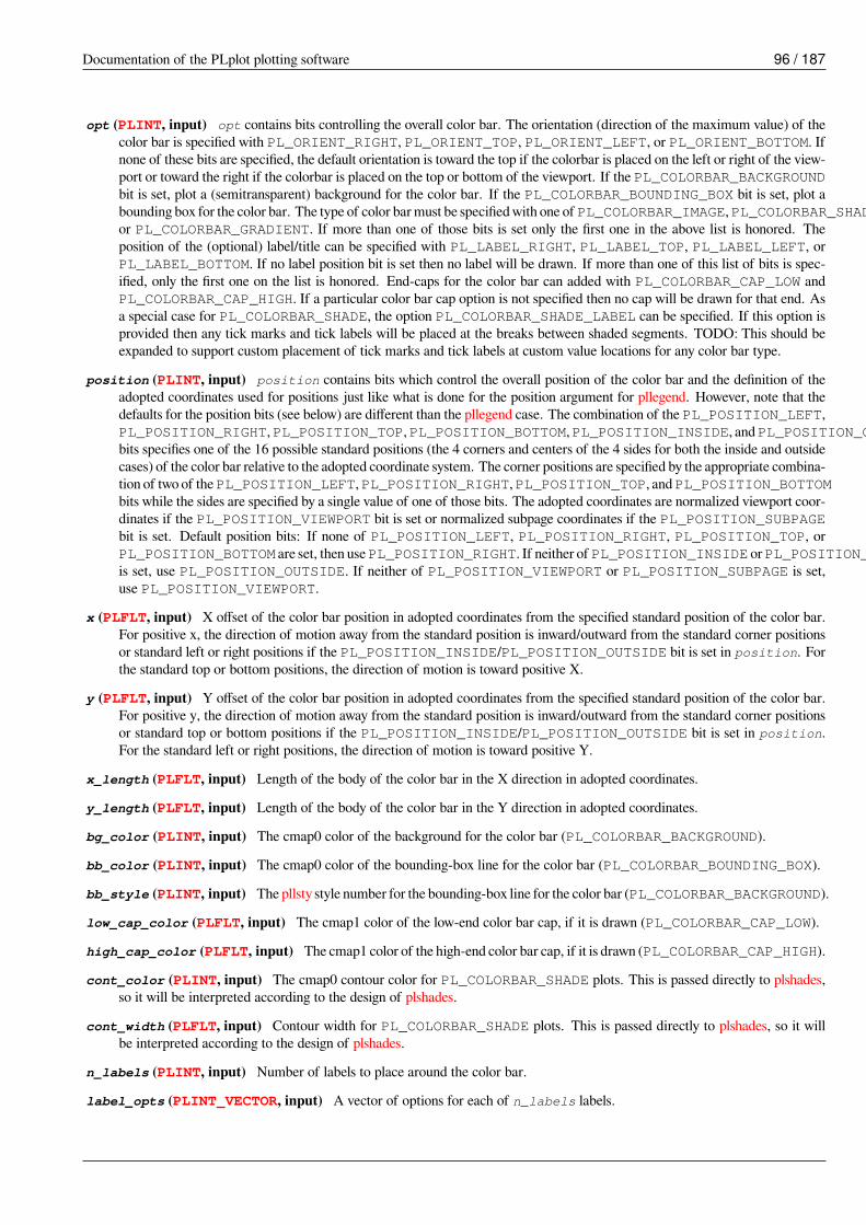
Documentation of the PLplot plotting software 96 / 187
opt (PLINT, input) opt contains bits controlling the overall color bar. The orientation (direction of the maximum value) of thecolor bar is specified with PL_ORIENT_RIGHT, PL_ORIENT_TOP, PL_ORIENT_LEFT, or PL_ORIENT_BOTTOM. Ifnone of these bits are specified, the default orientation is toward the top if the colorbar is placed on the left or right of the view-port or toward the right if the colorbar is placed on the top or bottom of the viewport. If the PL_COLORBAR_BACKGROUNDbit is set, plot a (semitransparent) background for the color bar. If the PL_COLORBAR_BOUNDING_BOX bit is set, plot abounding box for the color bar. The type of color barmust be specifiedwith one ofPL_COLORBAR_IMAGE,PL_COLORBAR_SHADE,or PL_COLORBAR_GRADIENT. If more than one of those bits is set only the first one in the above list is honored. Theposition of the (optional) label/title can be specified with PL_LABEL_RIGHT, PL_LABEL_TOP, PL_LABEL_LEFT, orPL_LABEL_BOTTOM. If no label position bit is set then no label will be drawn. If more than one of this list of bits is spec-ified, only the first one on the list is honored. End-caps for the color bar can added with PL_COLORBAR_CAP_LOW andPL_COLORBAR_CAP_HIGH. If a particular color bar cap option is not specified then no cap will be drawn for that end. Asa special case for PL_COLORBAR_SHADE, the option PL_COLORBAR_SHADE_LABEL can be specified. If this option isprovided then any tick marks and tick labels will be placed at the breaks between shaded segments. TODO: This should beexpanded to support custom placement of tick marks and tick labels at custom value locations for any color bar type.
position (PLINT, input) position contains bits which control the overall position of the color bar and the definition of theadopted coordinates used for positions just like what is done for the position argument for pllegend. However, note that thedefaults for the position bits (see below) are different than the pllegend case. The combination of the PL_POSITION_LEFT,PL_POSITION_RIGHT,PL_POSITION_TOP,PL_POSITION_BOTTOM,PL_POSITION_INSIDE, andPL_POSITION_OUTSIDEbits specifies one of the 16 possible standard positions (the 4 corners and centers of the 4 sides for both the inside and outsidecases) of the color bar relative to the adopted coordinate system. The corner positions are specified by the appropriate combina-tion of two of thePL_POSITION_LEFT,PL_POSITION_RIGHT,PL_POSITION_TOP, andPL_POSITION_BOTTOMbits while the sides are specified by a single value of one of those bits. The adopted coordinates are normalized viewport coor-dinates if the PL_POSITION_VIEWPORT bit is set or normalized subpage coordinates if the PL_POSITION_SUBPAGEbit is set. Default position bits: If none of PL_POSITION_LEFT, PL_POSITION_RIGHT, PL_POSITION_TOP, orPL_POSITION_BOTTOM are set, then usePL_POSITION_RIGHT. If neither ofPL_POSITION_INSIDE orPL_POSITION_OUTSIDEis set, use PL_POSITION_OUTSIDE. If neither of PL_POSITION_VIEWPORT or PL_POSITION_SUBPAGE is set,use PL_POSITION_VIEWPORT.
x (PLFLT, input) X offset of the color bar position in adopted coordinates from the specified standard position of the color bar.For positive x, the direction of motion away from the standard position is inward/outward from the standard corner positionsor standard left or right positions if the PL_POSITION_INSIDE/PL_POSITION_OUTSIDE bit is set in position. Forthe standard top or bottom positions, the direction of motion is toward positive X.
y (PLFLT, input) Y offset of the color bar position in adopted coordinates from the specified standard position of the color bar.For positive y, the direction of motion away from the standard position is inward/outward from the standard corner positionsor standard top or bottom positions if the PL_POSITION_INSIDE/PL_POSITION_OUTSIDE bit is set in position.For the standard left or right positions, the direction of motion is toward positive Y.
x_length (PLFLT, input) Length of the body of the color bar in the X direction in adopted coordinates.
y_length (PLFLT, input) Length of the body of the color bar in the Y direction in adopted coordinates.
bg_color (PLINT, input) The cmap0 color of the background for the color bar (PL_COLORBAR_BACKGROUND).
bb_color (PLINT, input) The cmap0 color of the bounding-box line for the color bar (PL_COLORBAR_BOUNDING_BOX).
bb_style (PLINT, input) The pllsty style number for the bounding-box line for the color bar (PL_COLORBAR_BACKGROUND).
low_cap_color (PLFLT, input) The cmap1 color of the low-end color bar cap, if it is drawn (PL_COLORBAR_CAP_LOW).
high_cap_color (PLFLT, input) The cmap1 color of the high-end color bar cap, if it is drawn (PL_COLORBAR_CAP_HIGH).
cont_color (PLINT, input) The cmap0 contour color for PL_COLORBAR_SHADE plots. This is passed directly to plshades,so it will be interpreted according to the design of plshades.
cont_width (PLFLT, input) Contour width for PL_COLORBAR_SHADE plots. This is passed directly to plshades, so it willbe interpreted according to the design of plshades.
n_labels (PLINT, input) Number of labels to place around the color bar.
label_opts (PLINT_VECTOR, input) A vector of options for each of n_labels labels.

Documentation of the PLplot plotting software 97 / 187
labels (PLCHAR_MATRIX, input) A vector of n_labels UTF-8 character strings containing the labels for the color bar.Ignored if no label position is specified with one of the PL_COLORBAR_LABEL_RIGHT, PL_COLORBAR_LABEL_TOP,PL_COLORBAR_LABEL_LEFT, or PL_COLORBAR_LABEL_BOTTOM bits in the corresponding label_opts field.
n_axes (PLINT, input) Number of axis definitions provided. This value must be greater than 0. It is typically 1 (numerical axislabels are provided for one of the long edges of the color bar), but it can be larger if multiple numerical axis labels for the longedges of the color bar are desired.
axis_opts (PLCHAR_MATRIX, input) A vector of n_axes ascii character strings containing options (interpreted as for plbox)for the color bar’s axis definitions.
ticks (PLFLT_VECTOR, input) A vector of n_axes values of the spacing of the major tick marks (interpreted as for plbox) forthe color bar’s axis definitions.
sub_ticks (PLINT_VECTOR, input) A vector of n_axes values of the number of subticks (interpreted as for plbox) for thecolor bar’s axis definitions.
n_values (PLINT_VECTOR, input) A vector containing the number of elements in each of the n_axes rows of the valuesmatrix.
values (PLFLT_MATRIX, input) Amatrix containing the numeric values for the data range represented by the color bar. For arow index of i_axis (where 0 < i_axis < n_axes), the number of elements in the row is specified by n_values[i_axis].For PL_COLORBAR_IMAGE and PL_COLORBAR_GRADIENT the number of elements is 2, and the corresponding row ele-ments of the valuesmatrix are theminimum andmaximumvalue represented by the colorbar. ForPL_COLORBAR_SHADE,the number and values of the elements of a row of the values matrix is interpreted the same as the nlevel and clevelarguments of plshades.
Redacted form: plcolorbar(p_colorbar_width, p_colorbar_height, opt, position, x, y, x_length,y_length, bg_color, bb_color, bb_style, low_cap_color, high_cap_color, cont_color, cont_width,label_opts, labels, axis_opts, ticks, sub_ticks, values)
This function is used in examples 16 and 33.
17.16 plconfigtime: Configure the transformation between continuousand broken-down time for the current stream
plconfigtime (scale, offset1, offset2, ccontrol, ifbtime_offset, year, month, day, hour, min, sec);Configure the transformation between continuous and broken-down time for the current stream. This transformation is used by bothplbtime and plctime.
scale (PLFLT, input) The number of days per continuous time unit. As a special case, if scale is 0., then all other argumentsare ignored, and the result (the default used by PLplot) is the equivalent of a call to plconfigtime(1./86400., 0., 0., 0x0, 1, 1970,0, 1, 0, 0, 0.). That is, for this special case broken-down time is calculated with the proleptic Gregorian calendar with no leapseconds inserted, and the continuous time is defined as the number of seconds since the Unix epoch of 1970-01-01T00:00:00Z.
offset1 (PLFLT, input) If ifbtime_offset is true, the parameters offset1 and offset2 are completely ignored. Other-wise, the sum of these parameters (with units in days) specify the epoch of the continuous time relative to the MJD epochcorresponding to the Gregorian calendar date of 1858-11-17T00:00:00Z or JD = 2400000.5. Two PLFLT numbers are usedto specify the origin to allow users (by specifying offset1 as an integer that can be exactly represented by a floating-pointvariable and specifying offset2 as a number in the range from 0. to 1) the chance to minimize the numerical errors of thecontinuous time representation.
offset2 (PLFLT, input) See documentation of offset1.
ccontrol (PLINT, input) ccontrol contains bits controlling the transformation. If the 0x1 bit is set, then the proleptic Juliancalendar is used for broken-down time rather than the proleptic Gregorian calendar. If the 0x2 bit is set, then leap seconds thathave been historically used to define UTC are inserted into the broken-down time. Other possibilities for additional controlbits for ccontrol exist such as making the historical time corrections in the broken-down time corresponding to ET (ephemeris

Documentation of the PLplot plotting software 98 / 187
time) or making the (slightly non-constant) corrections from international atomic time (TAI) to what astronomers define asterrestrial time (TT). But those additional possibilities have not been implemented yet in the qsastime library (one of thePLplot utility libraries).
ifbtime_offset (PLBOOL, input) ifbtime_offset controls how the epoch of the continuous time scale is specified by theuser. If ifbtime_offset is false, then offset1 and offset2 are used to specify the epoch, and the following broken-down time parameters are completely ignored. If ifbtime_offset is true, then offset1 and offset2 are completelyignored, and the following broken-down time parameters are used to specify the epoch.
year (PLINT, input) Year of epoch.
month (PLINT, input) Month of epoch in range from 0 (January) to 11 (December).
day (PLINT, input) Day of epoch in range from 1 to 31.
hour (PLINT, input) Hour of epoch in range from 0 to 23
min (PLINT, input) Minute of epoch in range from 0 to 59.
sec (PLFLT, input) Second of epoch in range from 0. to 60.
Redacted form:
• General: plconfigtime(scale, offset1, offset2, ccontrol, ifbtime_offset, year, month, day,hour, min, sec)
This function is used in example 29.
17.17 plcont: Contour plot
plcont (f, nx, ny, kx, lx, ky, ly, clevel, nlevel, pltr, pltr_data);Draws a contour plot of the data in f[nx][ny], using the nlevel contour levels specified by clevel. Only the region of thematrix from kx to lx and from ky to ly is plotted out where all these index ranges are interpreted as one-based for historical reasons.A transformation routine pointed to by pltr with a generic pointer pltr_data for additional data required by the transformationroutine is used to map indices within the matrix to the world coordinates.
f (PLFLT_MATRIX, input) A matrix containing data to be contoured.
nx, ny (PLINT, input) The dimensions of the matrix f.
kx, lx (PLINT, input) Range of x indices to consider where 0 ≤ kx-1 < lx-1 < nx. Values of kx and lx are one-based rather than zero-based for historical backwards-compatibility reasons.
ky, ly (PLINT, input) Range of y indices to consider where 0 ≤ ky-1 < ly-1 < ny. Values of ky and ly are one-based rather than zero-based for historical backwards-compatibility reasons.
clevel (PLFLT_VECTOR, input) A vector specifying the levels at which to draw contours.
nlevel (PLINT, input) Number of contour levels to draw.
pltr (PLTRANSFORM_callback, input) A callback function that defines the transformation between the zero-based indicesof the matrix f and the world coordinates.For the C case, transformation functions are provided in the PLplot library: pltr0 for the identity mapping, and pltr1 andpltr2 for arbitrary mappings respectively defined by vectors and matrices. In addition, C callback routines for the transforma-tion can be supplied by the user such as the mypltr function in examples/c/x09c.c which provides a general lineartransformation between index coordinates and world coordinates.For languages other than C you should consult Part III for the details concerning how PLTRANSFORM_callback argumentsare interfaced. However, in general, a particular pattern of callback-associated arguments such as a tr vector with 6 ele-ments; xg and yg vectors; or xg and yg matrices are respectively interfaced to a linear-transformation routine similar to

Documentation of the PLplot plotting software 99 / 187
the above mypltr function; pltr1; and pltr2. Furthermore, some of our more sophisticated bindings (see, e.g., Chapter 10)support native language callbacks for handling index to world-coordinate transformations. Examples of these various ap-proaches are given in examples/<language>x09*, examples/<language>x16*, examples/<language>x20*, examples/<language>x21*, and examples/<language>x22*, for all our supported languages.
pltr_data (PLPointer, input) Extra parameter to help pass information to pltr0, pltr1, pltr2, or whatever callback routinethat is externally supplied.
Redacted form: plcont(f, kx, lx, ky, ly, clevel, pltr, pltr_data)where (see above discussion) thepltr,pltr_data callback arguments are sometimes replaced by a tr vector with 6 elements; xg and yg vectors; or xg and yg matri-ces.This function is used in examples 9, 14, 16, and 22.
17.18 plcpstrm: Copy state parameters from the reference stream to thecurrent stream
plcpstrm (iplsr, flags);Copies state parameters from the reference stream to the current stream. Tell driver interface to map device coordinates unlessflags == 1.This function is used for making save files of selected plots (e.g. from the TK driver). After initializing, you can get a copy of thecurrent plot to the specified device by switching to this stream and issuing a plcpstrm and a plreplot, with calls to plbop and pleop asappropriate. The plot buffer must have previously been enabled (done automatically by some display drivers, such as X).
iplsr (PLINT, input) Number of reference stream.
flags (PLBOOL, input) If flags is set to true the device coordinates are not copied from the reference to current stream.
Redacted form: plcpstrm(iplsr, flags)
This function is used in example 1,20.
17.19 plctime: Calculate continuous time from broken-down time for thecurrent stream
plctime (year, month, day, hour, min, sec, ctime);Calculate continuous time, ctime, from broken-down time for the current stream. The broken-down time is specified by thefollowing parameters: year, month, day, hour, min, and sec. This function is the inverse of plbtime.The PLplot definition of broken-down time is a calendar time that completely ignores all time zone offsets, i.e., it is the user’sresponsibility to apply those offsets (if so desired) before using the PLplot time API. By default broken-down time is defined usingthe proleptic Gregorian calendar without the insertion of leap seconds and continuous time is defined as the number of secondssince the Unix epoch of 1970-01-01T00:00:00Z. However, other definitions of broken-down and continuous time are possible, seeplconfigtime which specifies that transformation for the current stream.
year (PLINT, input) Input year.
month (PLINT, input) Input month in range from 0 (January) to 11 (December).
day (PLINT, input) Input day in range from 1 to 31.
hour (PLINT, input) Input hour in range from 0 to 23
min (PLINT, input) Input minute in range from 0 to 59.

Documentation of the PLplot plotting software 100 / 187
sec (PLFLT, input) Input second in range from 0. to 60.
ctime (PLFLT_NC_SCALAR, output) Returned value of the continuous time calculated from the broken-down time specifiedby the previous parameters.
Redacted form:
• General: plctime(year, month, day, hour, min, sec, ctime)
This function is used in example 29.
17.20 plend: End plotting session
plend ();Ends a plotting session, tidies up all the output files, switches interactive devices back into text mode and frees up any memory thatwas allocated. Must be called before end of program.By default, PLplot’s interactive devices (Xwin, TK, etc.) go into a wait state after a call to plend or other functions which trigger theend of a plot page. To avoid this, use the plspause function.Redacted form: plend()This function is used in all of the examples.
17.21 plend1: End plotting session for current stream
plend1 ();Ends a plotting session for the current output stream only. See plsstrm for more info.Redacted form: plend1()This function is used in examples 1 and 20.
17.22 plenv0: Same as plenv but if in multiplot mode does not advancethe subpage, instead clears it
plenv0 (xmin, xmax, ymin, ymax, just, axis);Sets up plotter environment for simple graphs by calling pladv and setting up viewport and window to sensible default values. plenv0leaves a standard margin (left-hand margin of eight character heights, and a margin around the other three sides of five characterheights) around most graphs for axis labels and a title. When these defaults are not suitable, use the individual routines plvpas, plvpor,or plvasp for setting up the viewport, plwind for defining the window, and plbox for drawing the box.
xmin (PLFLT, input) Value of x at left-hand edge of window (in world coordinates).
xmax (PLFLT, input) Value of x at right-hand edge of window (in world coordinates).
ymin (PLFLT, input) Value of y at bottom edge of window (in world coordinates).
ymax (PLFLT, input) Value of y at top edge of window (in world coordinates).
just (PLINT, input) Controls how the axes will be scaled:
• -1: the scales will not be set, the user must set up the scale before calling plenv0 using plsvpa, plvasp or other.• 0: the x and y axes are scaled independently to use as much of the screen as possible.

Documentation of the PLplot plotting software 101 / 187
• 1: the scales of the x and y axes are made equal.• 2: the axis of the x and y axes are made equal, and the plot box will be square.
axis (PLINT, input) Controls drawing of the box around the plot:
• -2: draw no box, no tick marks, no numeric tick labels, no axes.• -1: draw box only.• 0: draw box, ticks, and numeric tick labels.• 1: also draw coordinate axes at x=0 and y=0.• 2: also draw a grid at major tick positions in both coordinates.• 3: also draw a grid at minor tick positions in both coordinates.• 10: same as 0 except logarithmic x tick marks. (The x data have to be converted to logarithms separately.)• 11: same as 1 except logarithmic x tick marks. (The x data have to be converted to logarithms separately.)• 12: same as 2 except logarithmic x tick marks. (The x data have to be converted to logarithms separately.)• 13: same as 3 except logarithmic x tick marks. (The x data have to be converted to logarithms separately.)• 20: same as 0 except logarithmic y tick marks. (The y data have to be converted to logarithms separately.)• 21: same as 1 except logarithmic y tick marks. (The y data have to be converted to logarithms separately.)• 22: same as 2 except logarithmic y tick marks. (The y data have to be converted to logarithms separately.)• 23: same as 3 except logarithmic y tick marks. (The y data have to be converted to logarithms separately.)• 30: same as 0 except logarithmic x and y tick marks. (The x and y data have to be converted to logarithms separately.)• 31: same as 1 except logarithmic x and y tick marks. (The x and y data have to be converted to logarithms separately.)• 32: same as 2 except logarithmic x and y tick marks. (The x and y data have to be converted to logarithms separately.)• 33: same as 3 except logarithmic x and y tick marks. (The x and y data have to be converted to logarithms separately.)• 40: same as 0 except date / time x labels.• 41: same as 1 except date / time x labels.• 42: same as 2 except date / time x labels.• 43: same as 3 except date / time x labels.• 50: same as 0 except date / time y labels.• 51: same as 1 except date / time y labels.• 52: same as 2 except date / time y labels.• 53: same as 3 except date / time y labels.• 60: same as 0 except date / time x and y labels.• 61: same as 1 except date / time x and y labels.• 62: same as 2 except date / time x and y labels.• 63: same as 3 except date / time x and y labels.• 70: same as 0 except custom x and y labels.• 71: same as 1 except custom x and y labels.• 72: same as 2 except custom x and y labels.• 73: same as 3 except custom x and y labels.
Redacted form: plenv0(xmin, xmax, ymin, ymax, just, axis)
This function is used in example 21.

Documentation of the PLplot plotting software 102 / 187
17.23 plenv: Set up standard window and draw box
plenv (xmin, xmax, ymin, ymax, just, axis);Sets up plotter environment for simple graphs by calling pladv and setting up viewport and window to sensible default values. plenvleaves a standard margin (left-hand margin of eight character heights, and a margin around the other three sides of five characterheights) around most graphs for axis labels and a title. When these defaults are not suitable, use the individual routines plvpas, plvpor,or plvasp for setting up the viewport, plwind for defining the window, and plbox for drawing the box.
xmin (PLFLT, input) Value of x at left-hand edge of window (in world coordinates).
xmax (PLFLT, input) Value of x at right-hand edge of window (in world coordinates).
ymin (PLFLT, input) Value of y at bottom edge of window (in world coordinates).
ymax (PLFLT, input) Value of y at top edge of window (in world coordinates).
just (PLINT, input) Controls how the axes will be scaled:
• -1: the scales will not be set, the user must set up the scale before calling plenv using plsvpa, plvasp or other.• 0: the x and y axes are scaled independently to use as much of the screen as possible.• 1: the scales of the x and y axes are made equal.• 2: the axis of the x and y axes are made equal, and the plot box will be square.
axis (PLINT, input) Controls drawing of the box around the plot:
• -2: draw no box, no tick marks, no numeric tick labels, no axes.• -1: draw box only.• 0: draw box, ticks, and numeric tick labels.• 1: also draw coordinate axes at x=0 and y=0.• 2: also draw a grid at major tick positions in both coordinates.• 3: also draw a grid at minor tick positions in both coordinates.• 10: same as 0 except logarithmic x tick marks. (The x data have to be converted to logarithms separately.)• 11: same as 1 except logarithmic x tick marks. (The x data have to be converted to logarithms separately.)• 12: same as 2 except logarithmic x tick marks. (The x data have to be converted to logarithms separately.)• 13: same as 3 except logarithmic x tick marks. (The x data have to be converted to logarithms separately.)• 20: same as 0 except logarithmic y tick marks. (The y data have to be converted to logarithms separately.)• 21: same as 1 except logarithmic y tick marks. (The y data have to be converted to logarithms separately.)• 22: same as 2 except logarithmic y tick marks. (The y data have to be converted to logarithms separately.)• 23: same as 3 except logarithmic y tick marks. (The y data have to be converted to logarithms separately.)• 30: same as 0 except logarithmic x and y tick marks. (The x and y data have to be converted to logarithms separately.)• 31: same as 1 except logarithmic x and y tick marks. (The x and y data have to be converted to logarithms separately.)• 32: same as 2 except logarithmic x and y tick marks. (The x and y data have to be converted to logarithms separately.)• 33: same as 3 except logarithmic x and y tick marks. (The x and y data have to be converted to logarithms separately.)• 40: same as 0 except date / time x labels.• 41: same as 1 except date / time x labels.• 42: same as 2 except date / time x labels.• 43: same as 3 except date / time x labels.• 50: same as 0 except date / time y labels.• 51: same as 1 except date / time y labels.• 52: same as 2 except date / time y labels.

Documentation of the PLplot plotting software 103 / 187
• 53: same as 3 except date / time y labels.• 60: same as 0 except date / time x and y labels.• 61: same as 1 except date / time x and y labels.• 62: same as 2 except date / time x and y labels.• 63: same as 3 except date / time x and y labels.• 70: same as 0 except custom x and y labels.• 71: same as 1 except custom x and y labels.• 72: same as 2 except custom x and y labels.• 73: same as 3 except custom x and y labels.
Redacted form: plenv(xmin, xmax, ymin, ymax, just, axis)
This function is used in example 1,3,9,13,14,19-22,29.
17.24 pleop: Eject current page
pleop ();Clears the graphics screen of an interactive device, or ejects a page on a plotter. See plbop for more information.Redacted form: pleop()This function is used in example 2,14.
17.25 plerrx: Draw error bars in x direction
plerrx (n, xmin, xmax, y);Draws a set of n error bars in x direction, the i’th error bar extending from xmin[i] to xmax[i] at y coordinate y[i]. Theterminals of the error bars are of length equal to the minor tick length (settable using plsmin).
n (PLINT, input) Number of error bars to draw.
xmin (PLFLT_VECTOR, input) A vector containing the x coordinates of the left-hand endpoints of the error bars.
xmax (PLFLT_VECTOR, input) A vector containing the x coordinates of the right-hand endpoints of the error bars.
y (PLFLT_VECTOR, input) A vector containing the y coordinates of the error bars.
Redacted form:
• General: plerrx(xmin, ymax, y)
This function is used in example 29.
17.26 plerry: Draw error bars in the y direction
plerry (n, x, ymin, ymax);Draws a set of n error bars in the y direction, the i’th error bar extending from ymin[i] to ymax[i] at x coordinate x[i]. Theterminals of the error bars are of length equal to the minor tick length (settable using plsmin).
n (PLINT, input) Number of error bars to draw.

Documentation of the PLplot plotting software 104 / 187
x (PLFLT_VECTOR, input) A vector containing the x coordinates of the error bars.
ymin (PLFLT_VECTOR, input) A vector containing the y coordinates of the lower endpoints of the error bars.
ymax (PLFLT_VECTOR, input) A vector containing the y coordinates of the upper endpoints of the error bars.
Redacted form:
• General: plerry(x, ymin, ymax)
This function is used in example 29.
17.27 plfamadv: Advance to the next family file on the next new page
plfamadv ();Advance to the next family file on the next new page.Redacted form: plfamadv()This function is not used in any examples.
17.28 plfill: Draw filled polygon
plfill (n, x, y);Fills the polygon defined by the n points (x[i], y[i]) using the pattern defined by plpsty or plpat. The default fill style is a solidfill. The routine will automatically close the polygon between the last and first vertices. If multiple closed polygons are passed in xand y then plfill will fill in between them.
n (PLINT, input) Number of vertices in polygon.
x (PLFLT_VECTOR, input) A vector containing the x coordinates of vertices.
y (PLFLT_VECTOR, input) A vector containing the y coordinates of vertices.
Redacted form: plfill(x,y)This function is used in examples 12, 13, 15, 16, 21, 24, and 25.
17.29 plfill3: Draw filled polygon in 3D
plfill3 (n, x, y, z);Fills the 3D polygon defined by the n points in the x, y, and z vectors using the pattern defined by plpsty or plpat. The routine willautomatically close the polygon between the last and first vertices. If multiple closed polygons are passed in x, y, and z then plfill3will fill in between them.
n (PLINT, input) Number of vertices in polygon.
x (PLFLT_VECTOR, input) A vector containing the x coordinates of vertices.
y (PLFLT_VECTOR, input) A vector containing the y coordinates of vertices.
z (PLFLT_VECTOR, input) A vector containing the z coordinates of vertices.
Redacted form:
• General: plfill3(x, y, z)
This function is used in example 15.

Documentation of the PLplot plotting software 105 / 187
17.30 plflush: Flushes the output stream
plflush ();Flushes the output stream. Use sparingly, if at all.Redacted form: plflush()This function is used in examples 1 and 14.
17.31 plfont: Set font
plfont (ifont);Sets the font used for subsequent text and symbols. For devices that still use Hershey fonts this routine has no effect unless theHershey fonts with extended character set are loaded (see plfontld). For unicode-aware devices that use system fonts instead ofHershey fonts, this routine calls the plsfci routine with argument set up appropriately for the various cases below. However, thismethod of specifying the font for unicode-aware devices is deprecated, and the much more flexible method of calling plsfont directlyis recommended instead (where plsfont provides a user-friendly interface to plsfci),
ifont (PLINT, input) Specifies the font:
• 1: Sans serif font (simplest and fastest)• 2: Serif font• 3: Italic font• 4: Script font
Redacted form: plfont(ifont)This function is used in examples 1, 2, 4, 7, 13, 24, and 26.
17.32 plfontld: Load Hershey fonts
plfontld (fnt);Loads the Hershey fonts used for text and symbols. This routine may be called before or after initializing PLplot. If not explicitlycalled before PLplot initialization, then by default that initialization loads Hershey fonts with the extended character set. This routineonly has a practical effect for devices that still use Hershey fonts (as opposed to modern devices that use unicode-aware system fontsinstead of Hershey fonts).
fnt (PLINT, input) Specifies the type of Hershey fonts to load. A zero value specifies Hershey fonts with the standard characterset and a non-zero value (the default assumed if plfontld is never called) specifies Hershey fonts with the extended characterset.
Redacted form: plfontld(fnt)This function is used in examples 1 and 7.
17.33 plGetCursor: Wait for graphics input event and translate to worldcoordinates.
PLINT plGetCursor (gin);Wait for graphics input event and translate to world coordinates. Returns 0 if no translation to world coordinates is possible.

Documentation of the PLplot plotting software 106 / 187
gin (PLGraphicsIn *, output) Pointer to PLGraphicsIn structure which will contain the output. The structure is not allo-cated by the routine and must exist before the function is called.
This function returns 1 on success and 0 if no translation to world coordinates is possible.Redacted form: plGetCursor(gin)This function is used in examples 1 and 20.
17.34 plgchr: Get character default height and current (scaled) height
plgchr (p_def, p_ht);Get character default height and current (scaled) height.
p_def (PLFLT_NC_SCALAR, output) Returned value of the default character height (mm).
p_ht (PLFLT_NC_SCALAR, output) Returned value of the scaled character height (mm).
Redacted form: plgchr(p_def, p_ht)
This function is used in example 23.
17.35 plgcmap1_range: Get the cmap1 argument range for continuouscolor plots
plgcmap1_range (min_color, max_color);Get the cmap1 argument range for continuous color plots. (Use plscmap1_range to set the cmap1 argument range.)
min_color (PLFLT_NC_SCALAR, output) Returned value of the current minimum cmap1 argument.
max_color (PLFLT_NC_SCALAR, output) Returned value of the current maximum cmap1 argument.
Redacted form: plgcmap1_range(min_color, max_color)
This function is currently not used in any example.
17.36 plgcol0: Returns 8-bit RGB values for given color index fromcmap0
plgcol0 (icol0, r, g, b);Returns 8-bit RGB values (0-255) for given color from cmap0 (see Section 3.7.1). Values are negative if an invalid color id is given.
icol0 (PLINT, input) Index of desired cmap0 color.
r (PLINT_NC_SCALAR, output) Returned value of the 8-bit red value.
g (PLINT_NC_SCALAR, output) Returned value of the 8-bit green value.
b (PLINT_NC_SCALAR, output) Returned value of the 8-bit blue value.
Redacted form: plgcol0(icol0, r, g, b)
This function is used in example 2.

Documentation of the PLplot plotting software 107 / 187
17.37 plgcol0a: Returns 8-bit RGB values andPLFLT alpha transparencyvalue for given color index from cmap0
plgcol0a (icol0, r, g, b, alpha);Returns 8-bit RGB values (0-255) and PLFLT alpha transparency value (0.0-1.0) for given color from cmap0 (see Section 3.7.1).Values are negative if an invalid color id is given.
icol0 (PLINT, input) Index of desired cmap0 color.
r (PLINT_NC_SCALAR, output) Returned value of the red intensity in the range from 0 to 255.
g (PLINT_NC_SCALAR, output) Returned value of the green intensity in the range from 0 to 255.
b (PLINT_NC_SCALAR, output) Returned value of the blue intensity in the range from 0 to 255.
alpha (PLFLT_NC_SCALAR, output) Returned value of the alpha transparency in the range from (0.0-1.0).
Redacted form: plgcola(r, g, b)
This function is used in example 30.
17.38 plgcolbg: Returns the background color (cmap0[0]) by 8-bit RGBvalue
plgcolbg (r, g, b);Returns the background color (cmap0[0]) by 8-bit RGB value.
r (PLINT_NC_SCALAR, output) Returned value of the red intensity in the range from 0 to 255.
g (PLINT_NC_SCALAR, output) Returned value of the green intensity in the range from 0 to 255.
b (PLINT_NC_SCALAR, output) Returned value of the blue intensity in the range from 0 to 255.
Redacted form: plgcolbg(r, g, b)
This function is used in example 31.
17.39 plgcolbga: Returns the background color (cmap0[0]) by 8-bit RGBvalue and PLFLT alpha transparency value
plgcolbga (r, g, b, alpha);Returns the background color (cmap0[0]) by 8-bit RGB value and PLFLT alpha transparency value.
r (PLINT_NC_SCALAR, output) Returned value of the red intensity in the range from 0 to 255.
g (PLINT_NC_SCALAR, output) Returned value of the green intensity in the range from 0 to 255.
b (PLINT_NC_SCALAR, output) Returned value of the blue intensity in the range from 0 to 255.
alpha (PLFLT_NC_SCALAR, output) Returned value of the alpha transparency in the range (0.0-1.0).
This function is used in example 31.

Documentation of the PLplot plotting software 108 / 187
17.40 plgcompression: Get the current device-compression setting
plgcompression (compression);Get the current device-compression setting. This parameter is only used for drivers that provide compression.
compression (PLINT_NC_SCALAR, output) Returned value of the compression setting for the current device.
Redacted form: plgcompression(compression)This function is used in example 31.
17.41 plgdev: Get the current device (keyword) name
plgdev (p_dev);Get the current device (keyword) name. Note: you must have allocated space for this (80 characters is safe).
p_dev (PLCHAR_NC_VECTOR, output) Returned ascii character string (with preallocated length of 80 characters or more)containing the device (keyword) name.
Redacted form: plgdev(p_dev)This function is used in example 14.
17.42 plgdidev: Get parameters that define current device-space win-dow
plgdidev (p_mar, p_aspect, p_jx, p_jy);Get relative margin width, aspect ratio, and relative justification that define current device-space window. If plsdidev has not beencalled the default values pointed to by p_mar, p_aspect, p_jx, and p_jy will all be 0.
p_mar (PLFLT_NC_SCALAR, output) Returned value of the relative margin width.
p_aspect (PLFLT_NC_SCALAR, output) Returned value of the aspect ratio.
p_jx (PLFLT_NC_SCALAR, output) Returned value of the relative justification in x.
p_jy (PLFLT_NC_SCALAR, output) Returned value of the relative justification in y.
Redacted form: plgdidev(p_mar, p_aspect, p_jx, p_jy)
This function is used in example 31.
17.43 plgdiori: Get plot orientation
plgdiori (p_rot);Get plot orientation parameter which is multiplied by 90° to obtain the angle of rotation. Note, arbitrary rotation parameters suchas 0.2 (corresponding to 18°) are possible, but the usual values for the rotation parameter are 0., 1., 2., and 3. corresponding to 0°(landscape mode), 90° (portrait mode), 180° (seascape mode), and 270° (upside-down mode). If plsdiori has not been called thedefault value pointed to by p_rot will be 0.
p_rot (PLFLT_NC_SCALAR, output) Returned value of the orientation parameter.
Redacted form: plgdiori(p_rot)This function is not used in any examples.

Documentation of the PLplot plotting software 109 / 187
17.44 plgdiplt: Get parameters that define current plot-space window
plgdiplt (p_xmin, p_ymin, p_xmax, p_ymax);Get relative minima and maxima that define current plot-space window. If plsdiplt has not been called the default values pointed toby p_xmin, p_ymin, p_xmax, and p_ymax will be 0., 0., 1., and 1.
p_xmin (PLFLT_NC_SCALAR, output) Returned value of the relative minimum in x.
p_ymin (PLFLT_NC_SCALAR, output) Returned value of the relative minimum in y.
p_xmax (PLFLT_NC_SCALAR, output) Returned value of the relative maximum in x.
p_ymax (PLFLT_NC_SCALAR, output) Returned value of the relative maximum in y.
Redacted form: plgdiplt(p_xmin, p_ymin, p_xmax, p_ymax)
This function is used in example 31.
17.45 plgdrawmode: Get drawing mode (depends on device support!)
plgdrawmode ();Get drawing mode. Note only one device driver (cairo) currently supports this at the moment, and for that case the PLINTvalue returned by this function is one of PL_DRAWMODE_DEFAULT, PL_DRAWMODE_REPLACE, PL_DRAWMODE_XOR, orPL_DRAWMODE_UNKNOWN. This function returns PL_DRAWMODE_UNKNOWN for the rest of the device drivers. See also pls-drawmode.Redacted form: plgdrawmode()This function is used in example 34.
17.46 plgfam: Get family file parameters
plgfam (p_fam, p_num, p_bmax);Gets information about current family file, if familying is enabled. See Section 3.2.2 for more information.
p_fam (PLINT_NC_SCALAR, output) Returned value of the current family flag value. If nonzero, familying is enabled for thecurrent device.
p_num (PLINT_NC_SCALAR, output) Returned value of the current family file number.
p_bmax (PLINT_NC_SCALAR, output) Returned value of the maximum file size (in bytes) for a family file.
Redacted form: plgfam(p_fam, p_num, p_bmax)
This function is used in examples 14 and 31.
17.47 plgfci: Get FCI (font characterization integer)
plgfci (p_fci);Gets information about the current font using the FCI approach. See Section 3.8.3 for more information.
p_fci (PLUNICODE_NC_SCALAR, output) Returned value of the current FCI value.
Redacted form: plgfci(p_fci)This function is used in example 23.

Documentation of the PLplot plotting software 110 / 187
17.48 plgfnam: Get output file name
plgfnam (fnam);Gets the current output file name, if applicable.
fnam (PLCHAR_NC_VECTOR, output) Returned ascii character string (with preallocated length of 80 characters or more) con-taining the file name.
Redacted form: plgfnam(fnam)This function is used in example 31.
17.49 plgfont: Get family, style and weight of the current font
plgfont (p_family, p_style, p_weight);Gets information about current font. See Section 3.8.3 for more information on font selection.
p_family (PLINT_NC_SCALAR, output) Returned value of the current font family. The available values are given by thePL_FCI_* constants inplplot.h. Current options are PL_FCI_SANS, PL_FCI_SERIF, PL_FCI_MONO, PL_FCI_SCRIPTand PL_FCI_SYMBOL. If p_family is NULL then the font family is not returned.
p_style (PLINT_NC_SCALAR, output) Returned value of the current font style. The available values are given by the PL_FCI_*constants in plplot.h. Current options are PL_FCI_UPRIGHT, PL_FCI_ITALIC and PL_FCI_OBLIQUE. If p_style isNULL then the font style is not returned.
p_weight (PLINT_NC_SCALAR, output) Returned value of the current font weight. The available values are given by thePL_FCI_* constants in plplot.h. Current options are PL_FCI_MEDIUM and PL_FCI_BOLD. If p_weight is NULLthen the font weight is not returned.
Redacted form: plgfont(p_family, p_style, p_weight)
This function is used in example 23.
17.50 plglevel: Get the (current) run level
plglevel (p_level);Get the (current) run level. Valid settings are:
• 0, uninitialized
• 1, initialized
• 2, viewport defined
• 3, world coordinates defined
p_level (PLINT_NC_SCALAR, output) Returned value of the run level.
Redacted form: plglevel(p_level)This function is used in example 31.

Documentation of the PLplot plotting software 111 / 187
17.51 plgpage: Get page parameters
plgpage (p_xp, p_yp, p_xleng, p_yleng, p_xoff, p_yoff);Gets the current page configuration. The length and offset values are expressed in units that are specific to the current driver. Forinstance: screen drivers will usually interpret them as number of pixels, whereas printer drivers will usually use mm.
p_xp (PLFLT_NC_SCALAR, output) Returned value of the number of pixels/inch (DPI) in x.
p_yp (PLFLT_NC_SCALAR, output) Returned value of the number of pixels/inch (DPI) in y.
p_xleng (PLINT_NC_SCALAR, output) Returned value of the x page length.
p_yleng (PLINT_NC_SCALAR, output) Returned value of the y page length.
p_xoff (PLINT_NC_SCALAR, output) Returned value of the x page offset.
p_yoff (PLINT_NC_SCALAR, output) Returned value of the y page offset.
Redacted form: plgpage(p_xp, p_yp, p_xleng, p_yleng, p_xoff, p_yoff)
This function is used in examples 14 and 31.
17.52 plgra: Switch to graphics screen
plgra ();Sets an interactive device to graphics mode, used in conjunction with pltext to allow graphics and text to be interspersed. On a devicewhich supports separate text and graphics windows, this command causes control to be switched to the graphics window. If alreadyin graphics mode, this command is ignored. It is also ignored on devices which only support a single window or use a differentmethod for shifting focus. See also pltext.Redacted form: plgra()This function is used in example 1.
17.53 plgradient: Draw linear gradient inside polygon
plgradient (n, x, y, angle);Draw a linear gradient using cmap1 inside the polygon defined by the n points (x[i], y[i]). Interpretation of the polygon isthe same as for plfill. The polygon coordinates and the gradient angle are all expressed in world coordinates. The angle from thex axis for both the rotated coordinate system and the gradient vector is specified by angle. The magnitude of the gradient vectoris the difference between the maximum and minimum values of x for the vertices in the rotated coordinate system. The origin ofthe gradient vector can be interpreted as being anywhere on the line corresponding to the minimum x value for the vertices in therotated coordinate system. The distance along the gradient vector is linearly transformed to the independent variable of color map1 which ranges from 0. at the tail of the gradient vector to 1. at the head of the gradient vector. What is drawn is the RGBA colorcorresponding to the independent variable of cmap1. For more information about cmap1 (see Section 3.7.2).
n (PLINT, input) Number of vertices in polygon.
x (PLFLT_VECTOR, input) A vector containing the x coordinates of vertices.
y (PLFLT_VECTOR, input) A vector containing the y coordinates of vertices.
angle (PLFLT, input) Angle (degrees) of gradient vector from x axis.
Redacted form: plgradient(x,y,angle)This function is used in examples 25 and 30.

Documentation of the PLplot plotting software 112 / 187
17.54 plgriddata: Grid data from irregularly sampled data
plgriddata (x, y, z, npts, xg, nptsx, yg, nptsy, zg, type, data);Real world data is frequently irregularly sampled, but PLplot 3D plots require data organized as a grid, i.e., with x sample pointvalues independent of y coordinate and vice versa. This function takes irregularly sampled data from the x[npts], y[npts],and z[npts] vectors; reads the desired grid location from the input vectors xg[nptsx] and yg[nptsy]; and returns theinterpolated result on that grid using the output matrix zg[nptsx][nptsy]. The algorithm used to interpolate the data to thegrid is specified with the argument type which can have one parameter specified in argument data.
x (PLFLT_VECTOR, input) The input x vector.
y (PLFLT_VECTOR, input) The input y vector.
z (PLFLT_VECTOR, input) The input z vector. Each triple x[i], y[i], z[i] represents one data sample coordinate.
npts (PLINT, input) The number of data samples in the x, y and z vectors.
xg (PLFLT_VECTOR, input) A vector that specifies the grid spacing in the x direction. Usually xg has nptsx equally spacedvalues from the minimum to the maximum values of the x input vector.
nptsx (PLINT, input) The number of points in the xg vector.
yg (PLFLT_VECTOR, input) A vector that specifies the grid spacing in the y direction. Similar to the xg parameter.
nptsy (PLINT, input) The number of points in the yg vector.
zg (PLFLT_NC_MATRIX, output) The matrix of interpolated results where data lies in the grid specified by xg and yg. There-fore the zg matrix must be dimensioned nptsx by nptsy.
type (PLINT, input) The type of grid interpolation algorithm to use, which can be:
• GRID_CSA: Bivariate Cubic Spline approximation• GRID_DTLI: Delaunay Triangulation Linear Interpolation• GRID_NNI: Natural Neighbors Interpolation• GRID_NNIDW: Nearest Neighbors Inverse Distance Weighted• GRID_NNLI: Nearest Neighbors Linear Interpolation• GRID_NNAIDW: Nearest Neighbors Around Inverse Distance Weighted
For details of the algorithms read the source file plgridd.c.
data (PLFLT, input) Some gridding algorithms require extra data, which can be specified through this argument. Currently, foralgorithm:
• GRID_NNIDW, data specifies the number of neighbors to use, the lower the value, the noisier (more local) the approxi-mation is.
• GRID_NNLI, data specifies what a thin triangle is, in the range [1. .. 2.]. High values enable the usage of very thintriangles for interpolation, possibly resulting in error in the approximation.
• GRID_NNI, only weights greater than data will be accepted. If 0, all weights will be accepted.
Redacted form:
• General: plgriddata(x, y, z, xg, yg, zg, type, data)
• Python: zg=plgriddata(x, y, z, xg, yg, type, data)
This function is used in example 21.

Documentation of the PLplot plotting software 113 / 187
17.55 plgspa: Get current subpage parameters
plgspa (xmin, xmax, ymin, ymax);Gets the size of the current subpage in millimeters measured from the bottom left hand corner of the output device page or screen.Can be used in conjunction with plsvpa for setting the size of a viewport in absolute coordinates (millimeters).
xmin (PLFLT_NC_SCALAR, output) Returned value of the position of the left hand edge of the subpage in millimeters.xmax (PLFLT_NC_SCALAR, output) Returned value of the position of the right hand edge of the subpage in millimeters.ymin (PLFLT_NC_SCALAR, output) Returned value of the position of the bottom edge of the subpage in millimeters.ymax (PLFLT_NC_SCALAR, output) Returned value of the position of the top edge of the subpage in millimeters.
Redacted form: plgspa(xmin, xmax, ymin, ymax)
This function is used in example 23.
17.56 plgstrm: Get current stream number
plgstrm (p_strm);Gets the number of the current output stream. See also plsstrm.
p_strm (PLINT_NC_SCALAR, output) Returned value of the current stream value.
Redacted form: plgstrm(p_strm)This function is used in example 1,20.
17.57 plgver: Get the current library version number
plgver (p_ver);Get the current library version number. Note: you must have allocated space for this (80 characters is safe).
p_ver (PLCHAR_NC_VECTOR, output) Returned ascii character string (with preallocated length of 80 characters or more) con-taining the PLplot version number.
Redacted form: plgver(p_ver)This function is used in example 1.
17.58 plgvpd: Get viewport limits in normalized device coordinates
plgvpd (p_xmin, p_xmax, p_ymin, p_ymax);Get viewport limits in normalized device coordinates.
p_xmin (PLFLT_NC_SCALAR, output) Returned value of the lower viewport limit of the normalized device coordinate in x.p_xmax (PLFLT_NC_SCALAR, output) Returned value of the upper viewport limit of the normalized device coordinate in x.p_ymin (PLFLT_NC_SCALAR, output) Returned value of the lower viewport limit of the normalized device coordinate in y.p_ymax (PLFLT_NC_SCALAR, output) Returned value of the upper viewport limit of the normalized device coordinate in y.
Redacted form:
• General: plgvpd(p_xmin, p_xmax, p_ymin, p_ymax)
This function is used in example 31.

Documentation of the PLplot plotting software 114 / 187
17.59 plgvpw: Get viewport limits in world coordinates
plgvpw (p_xmin, p_xmax, p_ymin, p_ymax);Get viewport limits in world coordinates.
p_xmin (PLFLT_NC_SCALAR, output) Returned value of the lower viewport limit of the world coordinate in x.
p_xmax (PLFLT_NC_SCALAR, output) Returned value of the upper viewport limit of the world coordinate in x.
p_ymin (PLFLT_NC_SCALAR, output) Returned value of the lower viewport limit of the world coordinate in y.
p_ymax (PLFLT_NC_SCALAR, output) Returned value of the upper viewport limit of the world coordinate in y.
Redacted form:
• General: plgvpw(p_xmin, p_xmax, p_ymin, p_ymax)
This function is used in example 31.
17.60 plgxax: Get x axis parameters
plgxax (p_digmax, p_digits);Returns current values of the p_digmax and p_digits flags for the x axis. p_digits is updated after the plot is drawn, so thisroutine should only be called after the call to plbox (or plbox3) is complete. See Section 3.4.3 for more information.
p_digmax (PLINT_NC_SCALAR, output) Returned value of the maximum number of digits for the x axis. If nonzero, theprinted label has been switched to a floating-point representation when the number of digits exceeds this value.
p_digits (PLINT_NC_SCALAR, output) Returned value of the actual number of digits for the numeric labels (x axis) fromthe last plot.
Redacted form: plgxax(p_digmax, p_digits)
This function is used in example 31.
17.61 plgyax: Get y axis parameters
plgyax (p_digmax, p_digits);Identical to plgxax, except that arguments are flags for y axis. See the description of plgxax for more detail.
p_digmax (PLINT_NC_SCALAR, output) Returned value of the maximum number of digits for the y axis. If nonzero, theprinted label has been switched to a floating-point representation when the number of digits exceeds this value.
p_digits (PLINT_NC_SCALAR, output) Returned value of the actual number of digits for the numeric labels (y axis) fromthe last plot.
Redacted form: plgyax(p_digmax, p_digits)
This function is used in example 31.

Documentation of the PLplot plotting software 115 / 187
17.62 plgzax: Get z axis parameters
plgzax (p_digmax, p_digits);Identical to plgxax, except that arguments are flags for z axis. See the description of plgxax for more detail.
p_digmax (PLINT_NC_SCALAR, output) Returned value of the maximum number of digits for the z axis. If nonzero, theprinted label has been switched to a floating-point representation when the number of digits exceeds this value.
p_digits (PLINT_NC_SCALAR, output) Returned value of the actual number of digits for the numeric labels (z axis) fromthe last plot.
Redacted form: plgzax(p_digmax, p_digits)
This function is used in example 31.
17.63 plhist: Plot a histogram from unbinned data
plhist (n, data, datmin, datmax, nbin, opt);Plots a histogram from n data points stored in the data vector. This routine bins the data into nbin bins equally spaced betweendatmin and datmax, and calls plbin to draw the resulting histogram. Parameter opt allows, among other things, the histogrameither to be plotted in an existing window or causes plhist to call plenv with suitable limits before plotting the histogram.
n (PLINT, input) Number of data points.
data (PLFLT_VECTOR, input) A vector containing the values of the n data points.
datmin (PLFLT, input) Left-hand edge of lowest-valued bin.
datmax (PLFLT, input) Right-hand edge of highest-valued bin.
nbin (PLINT, input) Number of (equal-sized) bins into which to divide the interval xmin to xmax.
opt (PLINT, input) Is a combination of several flags:
• opt=PL_HIST_DEFAULT: The axes are automatically rescaled to fit the histogram data, the outer bins are expanded tofill up the entire x-axis, data outside the given extremes are assigned to the outer bins and bins of zero height are simplydrawn.
• opt=PL_HIST_NOSCALING|...: The existing axes are not rescaled to fit the histogram data, without this flag, plenvis called to set the world coordinates.
• opt=PL_HIST_IGNORE_OUTLIERS|...: Data outside the given extremes are not taken into account. This optionshould probably be combined with opt=PL_HIST_NOEXPAND|..., so as to properly present the data.
• opt=PL_HIST_NOEXPAND|...: The outer bins are drawn with equal size as the ones inside.• opt=PL_HIST_NOEMPTY|...: Bins with zero height are not drawn (there is a gap for such bins).
Redacted form: plhist(data, datmin, datmax, nbin, opt)
This function is used in example 5.

Documentation of the PLplot plotting software 116 / 187
17.64 plhlsrgb: Convert HLS color to RGB
plhlsrgb (h, l, s, p_r, p_g, p_b);Convert HLS color coordinates to RGB.
h (PLFLT, input) Hue in degrees (0.0-360.0) on the color cylinder.
l (PLFLT, input) Lightness expressed as a fraction (0.0-1.0) of the axis of the color cylinder.
s (PLFLT, input) Saturation expressed as a fraction (0.0-1.0) of the radius of the color cylinder.
p_r (PLFLT_NC_SCALAR, output) Returned value of the red intensity (0.0-1.0) of the color.
p_g (PLFLT_NC_SCALAR, output) Returned value of the green intensity (0.0-1.0) of the color.
p_b (PLFLT_NC_SCALAR, output) Returned value of the blue intensity (0.0-1.0) of the color.
Redacted form:
• General: plhlsrgb(h, l, s, p_r, p_g, p_b)
This function is used in example 2.
17.65 plimagefr: Plot a 2D matrix using cmap1
plimagefr (idata, nx, ny, xmin, xmax, ymin, ymax, zmin, zmax, valuemin, valuemax, pltr, pltr_data);Plot a 2D matrix using cmap1.
idata (PLFLT_MATRIX, input) A matrix of values (intensities) to plot. Should have dimensions of nx by ny.
nx, ny (PLINT, input) Dimensions of idata
xmin, xmax, ymin, ymax (PLFLT, input) See the discussion of pltr below for how these arguments are used (only for thespecial case when the callback function pltr is not supplied).
zmin, zmax (PLFLT, input) Only data between zmin and zmax (inclusive) will be plotted.
valuemin, valuemax (PLFLT, input) The minimum and maximum data values to use for value to color mappings. A datumequal to or less than valuemin will be plotted with color 0.0, while a datum equal to or greater than valuemax will be plottedwith color 1.0. Data between valuemin and valuemax map linearly to colors in the range (0.0-1.0).
pltr (PLTRANSFORM_callback, input) A callback function that defines the transformation between the zero-based indicesof the matrix idata and world coordinates. If pltr is not supplied (e.g., is set to NULL in the C case), then the x indicesof idata are mapped to the range xmin through xmax and the y indices of idata are mapped to the range ymin throughymax.For the C case, transformation functions are provided in the PLplot library: pltr0 for the identity mapping, and pltr1 andpltr2 for arbitrary mappings respectively defined by vectors and matrices. In addition, C callback routines for the transforma-tion can be supplied by the user such as the mypltr function in examples/c/x09c.c which provides a general lineartransformation between index coordinates and world coordinates.For languages other than C you should consult Part III for the details concerning how PLTRANSFORM_callback argumentsare interfaced. However, in general, a particular pattern of callback-associated arguments such as a tr vector with 6 ele-ments; xg and yg vectors; or xg and yg matrices are respectively interfaced to a linear-transformation routine similar tothe above mypltr function; pltr1; and pltr2. Furthermore, some of our more sophisticated bindings (see, e.g., Chapter 10)support native language callbacks for handling index to world-coordinate transformations. Examples of these various ap-proaches are given in examples/<language>x09*, examples/<language>x16*, examples/<language>x20*, examples/<language>x21*, and examples/<language>x22*, for all our supported languages.

Documentation of the PLplot plotting software 117 / 187
pltr_data (PLPointer, input) Extra parameter to help pass information to pltr0, pltr1, pltr2, or whatever routine is externallysupplied.
Redacted form:
• General: plimagefr(idata, xmin, xmax, ymin, ymax, zmin, zmax, valuemin, valuemax, pltr,pltr_data)
This function is used in example 20.
17.66 plimage: Plot a 2D matrix using cmap1 with automatic color ad-justment
plimage (idata, nx, ny, xmin, xmax, ymin, ymax, zmin, zmax, Dxmin, Dxmax, Dymin, Dymax);Plot a 2D matrix using the cmap1 palette. The color scale is automatically adjusted to use the maximum and minimum values inidata as valuemin and valuemax in a call to plimagefr.
idata (PLFLT_MATRIX, input) A matrix containing function values to plot. Should have dimensions of nx by ny.
nx, ny (PLINT, input) Dimensions of idata
xmin, xmax, ymin, ymax (PLFLT, input) Thex andy index ranges are linearly transformed to these world coordinate rangessuch that idata[0][0] corresponds to (xmin, ymin) and idata[nx - 1][ny - 1] corresponds to (xmax,ymax).
zmin, zmax (PLFLT, input) Only data between zmin and zmax (inclusive) will be plotted.
Dxmin, Dxmax, Dymin, Dymax (PLFLT, input) Plot only the window of points whose plot coordinates fall inside the windowof (Dxmin, Dymin) to (Dxmax, Dymax).
Redacted form:
• General: plimage(idata, xmin, xmax, ymin, ymax, zmin, zmax, Dxmin, Dxmax, Dymin, Dymax)
This function is used in example 20.
17.67 plinit: Initialize PLplot
plinit ();Initializing the plotting package. The program prompts for the device keyword or number of the desired output device. Hitting aRETURN in response to the prompt is the same as selecting the first device. plinit will issue no prompt if either the device wasspecified previously (via command line flag, the plsetopt function, or the plsdev function), or if only one device is enabled whenPLplot is installed. If subpages have been specified, the output device is divided into nx by ny subpages, each of which may be usedindependently. If plinit is called again during a program, the previously opened file will be closed. The subroutine pladv is used toadvance from one subpage to the next.Redacted form: plinit()This function is used in all of the examples.

Documentation of the PLplot plotting software 118 / 187
17.68 pljoin: Draw a line between two points
pljoin (x1, y1, x2, y2);Joins the point (x1, y1) to (x2, y2).
x1 (PLFLT, input) x coordinate of first point.
y1 (PLFLT, input) y coordinate of first point.
x2 (PLFLT, input) x coordinate of second point.
y2 (PLFLT, input) y coordinate of second point.
Redacted form: pljoin(x1,y1,x2,y2)This function is used in examples 3 and 14.
17.69 pllab: Simple routine to write labels
pllab (xlabel, ylabel, tlabel);Routine for writing simple labels. Use plmtex for more complex labels.
xlabel (PLCHAR_VECTOR, input) A UTF-8 character string specifying the label for the x axis.
ylabel (PLCHAR_VECTOR, input) A UTF-8 character string specifying the label for the y axis.
tlabel (PLCHAR_VECTOR, input) A UTF-8 character string specifying the title of the plot.
Redacted form: pllab(xlabel, ylabel, tlabel)
This function is used in examples 1, 5, 9, 12, 14-16, 20-22, and 29.
17.70 pllegend: Plot legend using discretely annotated filled boxes, lines,and/or lines of symbols
pllegend (p_legend_width, p_legend_height, opt, position, x, y, plot_width, bg_color, bb_color, bb_style, nrow, ncolumn, nle-gend, opt_array, text_offset, text_scale, text_spacing, test_justification, text_colors, text, box_colors, box_patterns, box_scales,box_line_widths, line_colors, line_styles, line_widths, symbol_colors, symbol_scales, symbol_numbers, symbols);Routine for creating a discrete plot legend with a plotted filled box, line, and/or line of symbols for each annotated legend entry. (Seeplcolorbar for similar functionality for creating continuous color bars.) The arguments of pllegend provide control over the locationand size of the legend as well as the location and characteristics of the elements (most of which are optional) within that legend.The resulting legend is clipped at the boundaries of the current subpage. (N.B. the adopted coordinate system used for some of theparameters is defined in the documentation of the position parameter.)
p_legend_width (PLFLT_NC_SCALAR, output) Returned value of the legend width in adopted coordinates. This quantity iscalculated from plot_width, text_offset, ncolumn (possibly modified inside the routine depending on nlegend andnrow), and the length (calculated internally) of the longest text string.
p_legend_height (PLFLT_NC_SCALAR, output) Returned value of the legend height in adopted coordinates. This quantityis calculated from text_scale, text_spacing, and nrow (possibly modified inside the routine depending on nlegendand nrow).

Documentation of the PLplot plotting software 119 / 187
opt (PLINT, input) opt contains bits controlling the overall legend. If the PL_LEGEND_TEXT_LEFT bit is set, put the textarea on the left of the legend and the plotted area on the right. Otherwise, put the text area on the right of the legend and theplotted area on the left. If the PL_LEGEND_BACKGROUND bit is set, plot a (semitransparent) background for the legend.If the PL_LEGEND_BOUNDING_BOX bit is set, plot a bounding box for the legend. If the PL_LEGEND_ROW_MAJOR bitis set and (both of the possibly internally transformed) nrow > 1 and ncolumn > 1, then plot the resulting array of legendentries in row-major order. Otherwise, plot the legend entries in column-major order.
position (PLINT, input) position contains bits which control the overall position of the legend and the definition of theadopted coordinates used for positions just like what is done for the position argument for plcolorbar. However, note that thedefaults for the position bits (see below) are different than the plcolorbar case. The combination of thePL_POSITION_LEFT,PL_POSITION_RIGHT,PL_POSITION_TOP,PL_POSITION_BOTTOM,PL_POSITION_INSIDE, andPL_POSITION_OUTSIDEbits specifies one of the 16 possible standard positions (the 4 corners and centers of the 4 sides for both the inside and outsidecases) of the legend relative to the adopted coordinate system. The corner positions are specified by the appropriate combina-tion of two of thePL_POSITION_LEFT,PL_POSITION_RIGHT,PL_POSITION_TOP, andPL_POSITION_BOTTOMbits while the sides are specified by a single value of one of those bits. The adopted coordinates are normalized viewport coor-dinates if the PL_POSITION_VIEWPORT bit is set or normalized subpage coordinates if the PL_POSITION_SUBPAGEbit is set. Default position bits: If none of PL_POSITION_LEFT, PL_POSITION_RIGHT, PL_POSITION_TOP, orPL_POSITION_BOTTOM are set, then use the combination of PL_POSITION_RIGHT and PL_POSITION_TOP. Ifneither of PL_POSITION_INSIDE or PL_POSITION_OUTSIDE is set, use PL_POSITION_INSIDE. If neither ofPL_POSITION_VIEWPORT or PL_POSITION_SUBPAGE is set, use PL_POSITION_VIEWPORT.
x (PLFLT, input) X offset of the legend position in adopted coordinates from the specified standard position of the legend. Forpositive x, the direction of motion away from the standard position is inward/outward from the standard corner positions orstandard left or right positions if the PL_POSITION_INSIDE/PL_POSITION_OUTSIDE bit is set in position. Forthe standard top or bottom positions, the direction of motion is toward positive X.
y (PLFLT, input) Y offset of the legend position in adopted coordinates from the specified standard position of the legend. Forpositive y, the direction of motion away from the standard position is inward/outward from the standard corner positions orstandard top or bottom positions if the PL_POSITION_INSIDE/PL_POSITION_OUTSIDE bit is set in position. Forthe standard left or right positions, the direction of motion is toward positive Y.
plot_width (PLFLT, input) Horizontal width in adopted coordinates of the plot area (where the colored boxes, lines, and/orlines of symbols are drawn) of the legend.
bg_color (PLINT, input) The cmap0 color of the background for the legend (PL_LEGEND_BACKGROUND).
bb_color (PLINT, input) The cmap0 color of the bounding-box line for the legend (PL_LEGEND_BOUNDING_BOX).
bb_style (PLINT, input) The pllsty style number for the bounding-box line for the legend (PL_LEGEND_BACKGROUND).
nrow (PLINT, input) The number of rows in the matrix used to render the nlegend legend entries. For internal transformationsof nrow, see further remarks under nlegend.
ncolumn (PLINT, input) The number of columns in the matrix used to render the nlegend legend entries. For internal trans-formations of ncolumn, see further remarks under nlegend.
nlegend (PLINT, input) Number of legend entries. The above nrow and ncolumn values are transformed internally to beconsistent with nlegend. If either nrow or ncolumn is non-positive it is replaced by 1. If the resulting product of nrowand ncolumn is less than nlegend, the smaller of the two (or nrow, if nrow == ncolumn) is increased so the product is>= nlegend. Thus, for example, the common nrow = 0, ncolumn = 0 case is transformed internally to nrow = nlegend,ncolumn = 1; i.e., the usual case of a legend rendered as a single column.
opt_array (PLINT_VECTOR, input) A vector of nlegend values of options to control each individual plotted area corre-sponding to a legend entry. If the PL_LEGEND_NONE bit is set, then nothing is plotted in the plotted area. If the PL_LEGEND_COLOR_BOX,PL_LEGEND_LINE, and/or PL_LEGEND_SYMBOL bits are set, the area corresponding to a legend entry is plotted with a coloredbox; a line; and/or a line of symbols.
text_offset (PLFLT, input) Offset of the text area from the plot area in units of character width.
text_scale (PLFLT, input) Character height scale for text annotations.
text_spacing (PLFLT, input) Vertical spacing in units of the character height from one legend entry to the next.

Documentation of the PLplot plotting software 120 / 187
text_justification (PLFLT, input) Justification parameter used for text justification. Themost common values of text_justificationare 0., 0.5, or 1. corresponding to a text that is left justified, centred, or right justified within the text area, but other valuesare allowed as well.
text_colors (PLINT_VECTOR, input) A vector containing nlegend cmap0 text colors.
text (PLCHAR_MATRIX, input) A vector of nlegend UTF-8 character strings containing the legend annotations.
box_colors (PLINT_VECTOR, input) Avector containing nlegend cmap0 colors for the discrete colored boxes (PL_LEGEND_COLOR_BOX).
box_patterns (PLINT_VECTOR, input) A vector containing nlegend patterns (plpsty indices) for the discrete colored boxes(PL_LEGEND_COLOR_BOX).
box_scales (PLFLT_VECTOR, input) A vector containing nlegend scales (units of fraction of character height) for the heightof the discrete colored boxes (PL_LEGEND_COLOR_BOX).
box_line_widths (PLFLT_VECTOR, input) Avector containing nlegend line widths for the patterns specified by box_patterns(PL_LEGEND_COLOR_BOX).
line_colors (PLINT_VECTOR, input) A vector containing nlegend cmap0 line colors (PL_LEGEND_LINE).
line_styles (PLINT_VECTOR, input) A vector containing nlegend line styles (plsty indices) (PL_LEGEND_LINE).
line_widths (PLFLT_VECTOR, input) A vector containing nlegend line widths (PL_LEGEND_LINE).
symbol_colors (PLINT_VECTOR, input) A vector containing nlegend cmap0 symbol colors (PL_LEGEND_SYMBOL).
symbol_scales (PLFLT_VECTOR, input) Avector containing nlegend scale values for the symbol height (PL_LEGEND_SYMBOL).
symbol_numbers (PLINT_VECTOR, input) A vector containing nlegend numbers of symbols to be drawn across the widthof the plotted area (PL_LEGEND_SYMBOL).
symbols (PLCHAR_MATRIX, input) Avector of nlegendUTF-8 character strings containing the legend symbols. (PL_LEGEND_SYMBOL).
Redacted form: pllegend(p_legend_width, p_legend_height, opt, position, x, y, plot_width,bg_color, bb_color, bb_style, nrow, ncolumn, opt_array, text_offset, text_scale, text_spacing,test_justification, text_colors, text, box_colors, box_patterns, box_scales, box_line_widths,line_colors, line_styles, line_widths, symbol_colors, symbol_scales, symbol_numbers, symbols)
This function is used in examples 4, 26, and 33.
17.71 pllightsource: Sets the 3D position of the light source
pllightsource (x, y, z);Sets the 3D position of the light source for use with plsurf3d and plsurf3dl
x (PLFLT, input) X-coordinate of the light source.
y (PLFLT, input) Y-coordinate of the light source.
z (PLFLT, input) Z-coordinate of the light source.
Redacted form: pllightsource(x, y, z)
This function is used in example 8.

Documentation of the PLplot plotting software 121 / 187
17.72 plline: Draw a line
plline (n, x, y);Draws line defined by n points in x and y.
n (PLINT, input) Number of points defining line.
x (PLFLT_VECTOR, input) A vector containing the x coordinates of points.
y (PLFLT_VECTOR, input) A vector containing the y coordinates of points.
Redacted form: plline(x, y)
This function is used in examples 1, 3, 4, 9, 12-14, 16, 18, 20, 22, 25-27, and 29.
17.73 plline3: Draw a line in 3 space
plline3 (n, x, y, z);Draws line in 3 space defined by n points in x, y, and z. You must first set up the viewport, the 2d viewing window (in worldcoordinates), and the 3d normalized coordinate box. See x18c.c for more info.
n (PLINT, input) Number of points defining line.
x (PLFLT_VECTOR, input) A vector containing the x coordinates of points.
y (PLFLT_VECTOR, input) A vector containing the y coordinates of points.
z (PLFLT_VECTOR, input) A vector containing the z coordinates of points.
Redacted form: plline3(x, y, z)
This function is used in example 18.
17.74 pllsty: Select line style
pllsty (lin);This sets the line style according to one of eight predefined patterns (also see plstyl).
lin (PLINT, input) Integer value between 1 and 8. Line style 1 is a continuous line, line style 2 is a line with short dashes andgaps, line style 3 is a line with long dashes and gaps, line style 4 has long dashes and short gaps and so on.
Redacted form: pllsty(lin)This function is used in examples 9, 12, 22, and 25.
17.75 plmap: Plot continental outline or shapefile data in world coordi-nates
plmap ( mapform , name , minx , maxx , miny , maxy );Plots continental outlines or shapefile data in world coordinates. A demonstration of how to use this function to create differentprojections can be found in examples/c/x19c. PLplot is provided with basic coastal outlines and USA state borders. To use the map

Documentation of the PLplot plotting software 122 / 187
functionality PLplot must be compiled with the shapelib library. Shapefiles have become a popular standard for geographical dataand data in this format can be easily found from a number of online sources. Shapefile data is actually provided as three or morefiles with the same filename, but different extensions. The .shp and .shx files are required for plotting Shapefile data with PLplot.PLplot currently supports the point, multipoint, polyline and polygon objects within shapefiles. However holes in polygons are notsupported. When plmap is used the type of object is derived from the shapefile, if you wish to override the type then use one of theother plmap variants. The built in maps have line data only.
mapform (PLMAPFORM_callback, input) A user supplied function to transform the original map data coordinates to a newcoordinate system. The PLplot-supplied map data is provided as latitudes and longitudes; other Shapefile data may be providedin other coordinate systems as can be found in their .prj plain text files. For example, by using this transform we can changefrom a longitude, latitude coordinate to a polar stereographic projection. Initially, x[0]..[n-1] are the original x coordinates(longitudes for the PLplot-supplied data) and y[0]..y[n-1] are the corresponding y coordinates (latitudes for the PLplot supplieddata). After the call to mapform(), x[] and y[] should be replaced by the corresponding plot coordinates. If no transform isdesired, mapform can be replaced by NULL.
name (PLCHAR_VECTOR, input) An ascii character string specifying the type of map plotted. This is either one of the PLplotbuilt-in maps or the file name of a set of Shapefile files without the file extensions. For the PLplot built-in maps the possiblevalues are:
• ”globe” -- continental outlines• ”usa” -- USA and state boundaries• ”cglobe” -- continental outlines and countries• ”usaglobe” -- USA, state boundaries and continental outlines
minx (PLFLT, input) The minimum x value of map elements to be drawn. The units must match the shapefile (built in maps aredegrees lat/lon). Objects in the file which do not encroach on the box defined by minx, maxx, miny, maxy will not be rendered.But note this is simply an optimisation, not a clipping so for objects with some points inside the box and some points outsidethe box all the points will be rendered. These parameters also define latitude and longitude wrapping for shapefiles using theseunits. Longitude points will be wrapped by integer multiples of 360 degrees to place them in the box. This allows the samedata to be used on plots from -180-180 or 0-360 longitude ranges. In fact if you plot from -180-540 you will get two cyclesof data drawn. The value of minx must be less than the value of maxx. Passing in a nan, max/-max floating point number or+/-infinity will case the bounding box from the shapefile to be used.
maxx (PLFLT, input) The maximum x value of map elements to be drawn - see minx.
miny (PLFLT, input) The minimum y value of map elements to be drawn - see minx.
maxy (PLFLT, input) The maximum y value of map elements to be drawn - see minx.
Redacted form: plmap(mapform, name, minx, maxx, miny, maxy)
This function is used in example 19.
17.76 plmapfill: Plot all or a subset of Shapefile data, filling the poly-gons
plmapfill ( mapform , name , minx , maxx , miny , maxy , plotentries , nplotentries );As per plmapline, however the items are filled in the same way as plfill.
mapform (PLMAPFORM_callback, input) A user supplied function to transform the coordinates given in the shapefile into aplot coordinate system. By using this transform, we can change from a longitude, latitude coordinate to a polar stereographicproject, for example. Initially, x[0]..[n-1] are the longitudes and y[0]..y[n-1] are the corresponding latitudes. After the call tomapform(), x[] and y[] should be replaced by the corresponding plot coordinates. If no transform is desired, mapform can bereplaced by NULL.

Documentation of the PLplot plotting software 123 / 187
name (PLCHAR_VECTOR, input) An ascii character string specifying the file name of a set of Shapefile files without the fileextension.
minx (PLFLT, input) The minimum x value to be plotted. This must be in the same units as used by the Shapefile. You coulduse a very large negative number to plot everything, but you can improve performance by limiting the area drawn. The unitsmust match those of the Shapefile projection, which may be for example longitude or distance. The value of minx must beless than the value of maxx.
maxx (PLFLT, input) The maximum x value to be plotted. You could use a very large number to plot everything, but you canimprove performance by limiting the area drawn.
miny (PLFLT, input) The minimum y value to be plotted. This must be in the same units as used by the Shapefile. You coulduse a very large negative number to plot everything, but you can improve performance by limiting the area drawn. The unitsmust match those of the Shapefile projection, which may be for example latitude or distance. The value of miny must be lessthan the value of maxy.
maxy (PLFLT, input) The maximum y value to be plotted. You could use a very large number to plot everything, but you canimprove performance by limiting the area drawn.
plotentries (PLINT_VECTOR, input) A vector containing the zero-based indices of the Shapefile elements which will bedrawn. Setting plotentries to NULL will plot all elements of the Shapefile.
nplotentries (PLINT, input) The number of items in plotentries. Ignored if plotentries is NULL.
Redacted form: plmapfill(mapform, name, minx, maxx, miny, maxy, plotentries)
This function is used in example 19.
17.77 plmapline: Plot all or a subset of Shapefile data using lines inworld coordinates
plmapline ( mapform , name , minx , maxx , miny , maxy , plotentries , nplotentries );Plot all or a subset of Shapefile data using lines in world coordinates. Our 19th standard example demonstrates how to use thisfunction. This function plots data from a Shapefile using lines as in plmap, however it also has the option of also only drawingspecified elements from the Shapefile. The vector of indices of the required elements are passed as a function argument. TheShapefile data should include a metadata file (extension.dbf) listing all items within the Shapefile. This file can be opened by mostpopular spreadsheet programs and can be used to decide which indices to pass to this function.
mapform (PLMAPFORM_callback, input) A user supplied function to transform the coordinates given in the shapefile into aplot coordinate system. By using this transform, we can change from a longitude, latitude coordinate to a polar stereographicproject, for example. Initially, x[0]..[n-1] are the longitudes and y[0]..y[n-1] are the corresponding latitudes. After the call tomapform(), x[] and y[] should be replaced by the corresponding plot coordinates. If no transform is desired, mapform can bereplaced by NULL.
name (PLCHAR_VECTOR, input) An ascii character string specifying the file name of a set of Shapefile files without the fileextension.
minx (PLFLT, input) The minimum x value to be plotted. This must be in the same units as used by the Shapefile. You coulduse a very large negative number to plot everything, but you can improve performance by limiting the area drawn. The unitsmust match those of the Shapefile projection, which may be for example longitude or distance. The value of minx must beless than the value of maxx.
maxx (PLFLT, input) The maximum x value to be plotted. You could use a very large number to plot everything, but you canimprove performance by limiting the area drawn.
miny (PLFLT, input) The minimum y value to be plotted. This must be in the same units as used by the Shapefile. You coulduse a very large negative number to plot everything, but you can improve performance by limiting the area drawn. The unitsmust match those of the Shapefile projection, which may be for example latitude or distance. The value of miny must be lessthan the value of maxy.

Documentation of the PLplot plotting software 124 / 187
maxy (PLFLT, input) The maximum y value to be plotted. You could use a very large number to plot everything, but you canimprove performance by limiting the area drawn.
plotentries (PLINT_VECTOR, input) A vector containing the zero-based indices of the Shapefile elements which will bedrawn. Setting plotentries to NULL will plot all elements of the Shapefile.
nplotentries (PLINT, input) The number of items in plotentries. Ignored if plotentries is NULL.
Redacted form: plmapline(mapform, name, minx, maxx, miny, maxy, plotentries)
This function is used in example 19.
17.78 plmapstring: Plot all or a subset of Shapefile data using stringsor points in world coordinates
plmapstring ( mapform , name , string , minx , maxx , miny , maxy , plotentries , nplotentries );As per plmapline, however the items are plotted as strings or points in the same way as plstring.
mapform (PLMAPFORM_callback, input) A user supplied function to transform the coordinates given in the shapefile into aplot coordinate system. By using this transform, we can change from a longitude, latitude coordinate to a polar stereographicproject, for example. Initially, x[0]..[n-1] are the longitudes and y[0]..y[n-1] are the corresponding latitudes. After the call tomapform(), x[] and y[] should be replaced by the corresponding plot coordinates. If no transform is desired, mapform can bereplaced by NULL.
name (PLCHAR_VECTOR, input) An ascii character string specifying the file name of a set of Shapefile files without the fileextension.
string (PLCHAR_VECTOR, input) A UTF-8 character string to be drawn.
minx (PLFLT, input) The minimum x value to be plotted. This must be in the same units as used by the Shapefile. You coulduse a very large negative number to plot everything, but you can improve performance by limiting the area drawn. The unitsmust match those of the Shapefile projection, which may be for example longitude or distance. The value of minx must beless than the value of maxx.
maxx (PLFLT, input) The maximum x value to be plotted. You could use a very large number to plot everything, but you canimprove performance by limiting the area drawn.
miny (PLFLT, input) The minimum y value to be plotted. This must be in the same units as used by the Shapefile. You coulduse a very large negative number to plot everything, but you can improve performance by limiting the area drawn. The unitsmust match those of the Shapefile projection, which may be for example latitude or distance. The value of miny must be lessthan the value of maxy.
maxy (PLFLT, input) The maximum y value to be plotted. You could use a very large number to plot everything, but you canimprove performance by limiting the area drawn.
plotentries (PLINT_VECTOR, input) A vector containing the zero-based indices of the Shapefile elements which will bedrawn. Setting plotentries to NULL will plot all elements of the Shapefile.
nplotentries (PLINT, input) The number of items in plotentries. Ignored if plotentries is NULL.
Redacted form: plmapstring(mapform, name, string, minx, maxx, miny, maxy, plotentries)
This function is not used in any examples.

Documentation of the PLplot plotting software 125 / 187
17.79 plmaptex: Draw text at points defined by Shapefile data in worldcoordinates
plmaptex ( mapform , name , dx , dy , just , text , minx , maxx , miny , maxy , plotentry );As per plmapline, however the items are plotted as text in the same way as plptex.
mapform (PLMAPFORM_callback, input) A user supplied function to transform the coordinates given in the shapefile into aplot coordinate system. By using this transform, we can change from a longitude, latitude coordinate to a polar stereographicproject, for example. Initially, x[0]..[n-1] are the longitudes and y[0]..y[n-1] are the corresponding latitudes. After the call tomapform(), x[] and y[] should be replaced by the corresponding plot coordinates. If no transform is desired, mapform can bereplaced by NULL.
name (PLCHAR_VECTOR, input) An ascii character string specifying the file name of a set of Shapefile files without the fileextension.
dx (PLFLT, input) Used to define the slope of the texts which is dy/dx.
dy (PLFLT, input) Used to define the slope of the texts which is dy/dx.
just (PLFLT, input) Set the justification of the text. The value given will be the fraction of the distance along the string that sitsat the given point. 0.0 gives left aligned text, 0.5 gives centralized text and 1.0 gives right aligned text.
text (PLCHAR_VECTOR, input) A UTF-8 character string to be drawn.
minx (PLFLT, input) The minimum x value to be plotted. This must be in the same units as used by the Shapefile. You coulduse a very large negative number to plot everything, but you can improve performance by limiting the area drawn. The unitsmust match those of the Shapefile projection, which may be for example longitude or distance. The value of minx must beless than the value of maxx.
maxx (PLFLT, input) The maximum x value to be plotted. You could use a very large number to plot everything, but you canimprove performance by limiting the area drawn.
miny (PLFLT, input) The minimum y value to be plotted. This must be in the same units as used by the Shapefile. You coulduse a very large negative number to plot everything, but you can improve performance by limiting the area drawn. The unitsmust match those of the Shapefile projection, which may be for example latitude or distance. The value of miny must be lessthan the value of maxy.
maxy (PLFLT, input) The maximum y value to be plotted. You could use a very large number to plot everything, but you canimprove performance by limiting the area drawn.
plotentry (PLINT, input) An integer indicating which text string of the Shapefile (zero indexed) will be drawn.
Redacted form: plmaptex(mapform, name, dx, dy, just, text, minx, maxx, miny, maxy, plotentry)
This function is used in example 19.
17.80 plmeridians: Plot latitude and longitude lines
plmeridians ( mapform , dlong , dlat , minlong , maxlong , minlat , maxlat );Displays latitude and longitude on the current plot. The lines are plotted in the current color and line style.
mapform (PLMAPFORM_callback, input) A user supplied function to transform the coordinate longitudes and latitudes to aplot coordinate system. By using this transform, we can change from a longitude, latitude coordinate to a polar stereographicproject, for example. Initially, x[0]..[n-1] are the longitudes and y[0]..y[n-1] are the corresponding latitudes. After the call tomapform(), x[] and y[] should be replaced by the corresponding plot coordinates. If no transform is desired, mapform can bereplaced by NULL.

Documentation of the PLplot plotting software 126 / 187
dlong (PLFLT, input) The interval in degrees at which the longitude lines are to be plotted.
dlat (PLFLT, input) The interval in degrees at which the latitude lines are to be plotted.
minlong (PLFLT, input) The value of the longitude on the left side of the plot. The value of minlong must be less than the valueof maxlong, and the quantity maxlong-minlong must be less than or equal to 360.
maxlong (PLFLT, input) The value of the longitude on the right side of the plot.
minlat (PLFLT, input) The minimum latitude to be plotted on the background. One can always use -90.0 as the boundaryoutside the plot window will be automatically eliminated. However, the program will be faster if one can reduce the size ofthe background plotted.
maxlat (PLFLT, input) The maximum latitudes to be plotted on the background. One can always use 90.0 as the boundaryoutside the plot window will be automatically eliminated.
Redacted form: plmeridians(mapform, dlong, dlat, minlong, maxlong, minlat, maxlat)
This function is used in example 19.
17.81 plmesh: Plot surface mesh
plmesh ( x , y , z , nx , ny , opt );Plots a surface mesh within the environment set up by plw3d. The surface is defined by the matrix z[nx][ny] , the pointz[i][j] being the value of the function at (x[i], y[j]). Note that the points in vectors x and y do not need to be equallyspaced, but must be stored in ascending order. The parameter opt controls the way in which the surface is displayed. For furtherdetails see Section 3.9.
x (PLFLT_VECTOR, input) A vector containing the x coordinates at which the function is evaluated.
y (PLFLT_VECTOR, input) A vector containing the y coordinates at which the function is evaluated.
z (PLFLT_MATRIX, input) A matrix containing function values to plot. Should have dimensions of nx by ny.
nx (PLINT, input) Number of x values at which function has been evaluated.
ny (PLINT, input) Number of y values at which function has been evaluated.
opt (PLINT, input) Determines the way in which the surface is represented:
• opt=DRAW_LINEX : Lines are drawn showing z as a function of x for each value of y[j] .• opt=DRAW_LINEY : Lines are drawn showing z as a function of y for each value of x[i] .• opt=DRAW_LINEXY : Network of lines is drawn connecting points at which function is defined.
Redacted form: plmesh(x, y, z, opt)
This function is used in example 11.
17.82 plmeshc: Magnitude colored plot surface mesh with contour
plmeshc ( x , y , z , nx , ny , opt , clevel , nlevel );A more powerful form of plmesh: the surface mesh can be colored accordingly to the current z value being plotted, a contour plotcan be drawn at the base XY plane, and a curtain can be drawn between the plotted function border and the base XY plane.
x (PLFLT_VECTOR, input) A vector containing the x coordinates at which the function is evaluated.
y (PLFLT_VECTOR, input) A vector containing the y coordinates at which the function is evaluated.

Documentation of the PLplot plotting software 127 / 187
z (PLFLT_MATRIX, input) A matrix containing function values to plot. Should have dimensions of nx by ny.
nx (PLINT, input) Number of x values at which function is evaluated.
ny (PLINT, input) Number of y values at which function is evaluated.
opt (PLINT, input) Determines the way in which the surface is represented. To specify more than one option just add the options,e.g. DRAW_LINEXY + MAG_COLOR
• opt=DRAW_LINEX : Lines are drawn showing z as a function of x for each value of y[j] .• opt=DRAW_LINEY : Lines are drawn showing z as a function of y for each value of x[i] .• opt=DRAW_LINEXY : Network of lines is drawn connecting points at which function is defined.• opt=MAG_COLOR : Each line in the mesh is colored according to the z value being plotted. The color is used from thecurrent cmap1.
• opt=BASE_CONT : A contour plot is drawn at the base XY plane using parameters nlevel and clevel.• opt=DRAW_SIDES : draws a curtain between the base XY plane and the borders of the plotted function.
clevel (PLFLT_VECTOR, input) A vector containing the contour levels.
nlevel (PLINT, input) Number of elements in the clevel vector.
Redacted form: plmeshc(x, y, z, opt, clevel)
This function is used in example 11.
17.83 plmkstrm: Creates a new stream and makes it the default
plmkstrm ( p_strm );Creates a new stream and makes it the default. Differs from using plsstrm, in that a free stream number is found, and returned.Unfortunately, I have to start at stream 1 and work upward, since stream 0 is preallocated. One of the big flaws in the PLplot API isthat no initial, library-opening call is required. So stream 0 must be preallocated, and there is no simple way of determining whetherit is already in use or not.
p_strm (PLINT_NC_SCALAR, output) Returned value of the stream number of the created stream.
Redacted form: plmkstrm(p_strm)This function is used in examples 1 and 20.
17.84 plmtex: Write text relative to viewport boundaries
plmtex ( side , disp , pos , just , text );Writes text at a specified position relative to the viewport boundaries. Text may be written inside or outside the viewport, but isclipped at the subpage boundaries. The reference point of a string lies along a line passing through the string at half the height of acapital letter. The position of the reference point along this line is determined by just , and the position of the reference pointrelative to the viewport is set by disp and pos .
side (PLCHAR_VECTOR, input) An ascii character string specifying the side of the viewport along which the text is to be written.The string must be one of:
• b: Bottom of viewport, text written parallel to edge.• bv: Bottom of viewport, text written at right angles to edge.• l: Left of viewport, text written parallel to edge.

Documentation of the PLplot plotting software 128 / 187
• lv: Left of viewport, text written at right angles to edge.• r: Right of viewport, text written parallel to edge.• rv: Right of viewport, text written at right angles to edge.• t: Top of viewport, text written parallel to edge.• tv: Top of viewport, text written at right angles to edge.
disp (PLFLT, input) Position of the reference point of string, measured outwards from the specified viewport edge in units ofthe current character height. Use negative disp to write within the viewport.
pos (PLFLT, input) Position of the reference point of string along the specified edge, expressed as a fraction of the length of theedge.
just (PLFLT, input) Specifies the position of the string relative to its reference point. If just=0. , the reference point is atthe left and if just=1. , it is at the right of the string. Other values of just give intermediate justifications.
text (PLCHAR_VECTOR, input) A UTF-8 character string to be written out.
Redacted form:
• General: plmtex(side, disp, pos, just, text)
This function is used in examples 3, 4, 6-8, 11, 12, 14, 18, 23, and 26.
17.85 plmtex3: Write text relative to viewport boundaries in 3D plots
plmtex3 ( side , disp , pos , just , text );Writes text at a specified position relative to the viewport boundaries. Text may be written inside or outside the viewport, but isclipped at the subpage boundaries. The reference point of a string lies along a line passing through the string at half the height of acapital letter. The position of the reference point along this line is determined by just , and the position of the reference pointrelative to the viewport is set by disp and pos .
side (PLCHAR_VECTOR, input) An ascii character string specifying the side of the viewport along which the text is to be written.The string should contain one or more of the following characters: [xyz][ps][v]. Only one label is drawn at a time, i.e.xyp will only label the X axis, not both the X and Y axes.
• x: Label the X axis.• y: Label the Y axis.• z: Label the Z axis.• p: Label the “primary” axis. For Z this is the leftmost Z axis. For X it is the axis that starts at y-min. For Y it is the axisthat starts at x-min.
• s: Label the “secondary” axis.• v: Draw the text perpendicular to the axis.
disp (PLFLT, input) Position of the reference point of string, measured outwards from the specified viewport edge in units ofthe current character height. Use negative disp to write within the viewport.
pos (PLFLT, input) Position of the reference point of string along the specified edge, expressed as a fraction of the length of theedge.
just (PLFLT, input) Specifies the position of the string relative to its reference point. If just=0. , the reference point is atthe left and if just=1. , it is at the right of the string. Other values of just give intermediate justifications.
text (PLCHAR_VECTOR, input) A UTF-8 character string to be written out.
Redacted form: plmtex3(side, disp, pos, just, text)
This function is used in example 28.

Documentation of the PLplot plotting software 129 / 187
17.86 plot3d: Plot 3-d surface plot
plot3d ( x , y , z , nx , ny , opt , side );Plots a three-dimensional surface plot within the environment set up by plw3d. The surface is defined by the matrix z[nx][ny], the point z[i][j] being the value of the function at (x[i],y[j]). Note that the points in vectors x and y do not need to beequally spaced, but must be stored in ascending order. The parameter opt controls the way in which the surface is displayed. Forfurther details see Section 3.9. The only difference between plmesh and plot3d is that plmesh draws the bottom side of the surface,while plot3d only draws the surface as viewed from the top.
x (PLFLT_VECTOR, input) A vector containing the x coordinates at which the function is evaluated.
y (PLFLT_VECTOR, input) A vector containing the y coordinates at which the function is evaluated.
z (PLFLT_MATRIX, input) A matrix containing function values to plot. Should have dimensions of nx by ny.
nx (PLINT, input) Number of x values at which function is evaluated.
ny (PLINT, input) Number of y values at which function is evaluated.
opt (PLINT, input) Determines the way in which the surface is represented:
• opt=DRAW_LINEX : Lines are drawn showing z as a function of x for each value of y[j] .• opt=DRAW_LINEY : Lines are drawn showing z as a function of y for each value of x[i] .• opt=DRAW_LINEXY : Network of lines is drawn connecting points at which function is defined.
side (PLBOOL, input) Flag to indicate whether or not ̀ ̀sides” should be draw on the figure. If side is true sides are drawn,otherwise no sides are drawn.
Redacted form: plot3d(x, y, z, opt, side)
This function is used in examples 11 and 21.
17.87 plot3dc: Magnitude colored plot surface with contour
plot3dc ( x , y , z , nx , ny , opt , clevel , nlevel );Aside from dropping the side functionality this is a more powerful form of plot3d: the surface mesh can be colored accordinglyto the current z value being plotted, a contour plot can be drawn at the base XY plane, and a curtain can be drawn between theplotted function border and the base XY plane. The arguments are identical to those of plmeshc. The only difference betweenplmeshc and plot3dc is that plmeshc draws the bottom side of the surface, while plot3dc only draws the surface as viewed from thetop.
x (PLFLT_VECTOR, input) A vector containing the x coordinates at which the function is evaluated.
y (PLFLT_VECTOR, input) A vector containing the y coordinates at which the function is evaluated.
z (PLFLT_MATRIX, input) A matrix containing function values to plot. Should have dimensions of nx by ny.
nx (PLINT, input) Number of x values at which function is evaluated.
ny (PLINT, input) Number of y values at which function is evaluated.
opt (PLINT, input) Determines the way in which the surface is represented. To specify more than one option just add the options,e.g. DRAW_LINEXY + MAG_COLOR
• opt=DRAW_LINEX : Lines are drawn showing z as a function of x for each value of y[j] .• opt=DRAW_LINEY : Lines are drawn showing z as a function of y for each value of x[i] .• opt=DRAW_LINEXY : Network of lines is drawn connecting points at which function is defined.

Documentation of the PLplot plotting software 130 / 187
• opt=MAG_COLOR : Each line in the mesh is colored according to the z value being plotted. The color is used from thecurrent cmap1.
• opt=BASE_CONT : A contour plot is drawn at the base XY plane using parameters nlevel and clevel.• opt=DRAW_SIDES : draws a curtain between the base XY plane and the borders of the plotted function.
clevel (PLFLT_VECTOR, input) A vector containing the contour levels.
nlevel (PLINT, input) Number of elements in the clevel vector.
Redacted form:
• General: plot3dc(x, y, z, opt, clevel)
This function is used in example 21.
17.88 plot3dcl: Magnitude colored plot surface with contour for z[x][y]with y index limits
plot3dcl ( x , y , z , nx , ny , opt , clevel , nlevel , indexxmin , indexxmax , indexymin , indexymax );When the implementation is completed this variant of plot3dc (see that function’s documentation for more details) should be suitablefor the case where the area of the x, y coordinate grid where z is defined can be non-rectangular. The implementation is incompleteso the last 4 parameters of plot3dcl; indexxmin , indexxmax , indexymin , and indexymax ; are currently ignoredand the functionality is otherwise identical to that of plot3dc.
x (PLFLT_VECTOR, input) A vector containing the x coordinates at which the function is evaluated.
y (PLFLT_VECTOR, input) A vector containing the y coordinates at which the function is evaluated.
z (PLFLT_MATRIX, input) A matrix containing function values to plot. Should have dimensions of nx by ny.
nx (PLINT, input) Number of x values at which the function is evaluated.
ny (PLINT, input) Number of y values at which the function is evaluated.
opt (PLINT, input) Determines the way in which the surface is represented. To specify more than one option just add the options,e.g. DRAW_LINEXY + MAG_COLOR
• opt=DRAW_LINEX : Lines are drawn showing z as a function of x for each value of y[j] .• opt=DRAW_LINEY : Lines are drawn showing z as a function of y for each value of x[i] .• opt=DRAW_LINEXY : Network of lines is drawn connecting points at which function is defined.• opt=MAG_COLOR : Each line in the mesh is colored according to the z value being plotted. The color is used from thecurrent cmap1.
• opt=BASE_CONT : A contour plot is drawn at the base XY plane using parameters nlevel and clevel.• opt=DRAW_SIDES : draws a curtain between the base XY plane and the borders of the plotted function.
clevel (PLFLT_VECTOR, input) A vector containing the contour levels.
nlevel (PLINT, input) Number of elements in the clevel vector.
indexxmin (PLINT, input) The index value (which must be ≥ 0) that corresponds to the first x index where z is defined.
indexxmax (PLINT, input) The index value (which must be ≤ nx ) which corresponds (by convention) to one more than thelast x index value where z is defined.
indexymin (PLINT_VECTOR, input) A vector containing y index values which all must be ≥ 0. These values are the first yindex where z is defined for a particular x index in the range from indexxmin to indexxmax - 1. The dimension ofindexymin is indexxmax.

Documentation of the PLplot plotting software 131 / 187
indexymax (PLINT_VECTOR, input) A vector containing y index values which all must be ≤ ny. These values correspond (byconvention) to one more than the last y index where z is defined for a particular x index in the range from indexxmin toindexxmax - 1. The dimension of indexymax is indexxmax.
Redacted form:
• General: plot3dcl(x, y, z, opt, clevel, indexxmin, indexymin, indexymax)
This function is not used in any example.
17.89 plparseopts: Parse command-line arguments
PLINT plparseopts ( p_argc , argv , mode );Parse command-line arguments.plparseopts removes all recognized flags (decreasing argc accordingly), so that invalid input may be readily detected. It can also beused to process user command line flags. The user can merge an option table of type PLOptionTable into the internal option tableinfo structure using plMergeOpts. Or, the user can specify that ONLY the external table(s) be parsed by calling plClearOpts beforeplMergeOpts.The default action taken by plparseopts is as follows:Returns with an error if an unrecognized option or badly formed option-value pair are encountered.Returns immediately (return code 0) when the first non-option command line argument is found.Returns with the return code of the option handler, if one was called.Deletes command line arguments from argv list as they are found, and decrements argc accordingly.Does not show ”invisible” options in usage or help messages.Assumes the program name is contained in argv[0].
These behaviors may be controlled through the mode argument.
p_argc (int *, input/output) Number of arguments.
argv (PLCHAR_NC_MATRIX, input/output) A vector of character strings containing *p_argc command-line arguments.
mode (PLINT, input) Parsing mode with the following possibilities:
• PL_PARSE_FULL (1) -- Full parsing of command line and all error messages enabled, including program exit when anerror occurs. Anything on the command line that isn’t recognized as a valid option or option argument is flagged as an error.
• PL_PARSE_QUIET (2) -- Turns off all output except in the case of errors.• PL_PARSE_NODELETE (4) -- Turns off deletion of processed arguments.• PL_PARSE_SHOWALL (8) -- Show invisible options• PL_PARSE_NOPROGRAM (32) -- Specified if argv[0] is NOT a pointer to the program name.• PL_PARSE_NODASH (64) -- Set if leading dash is NOT required.• PL_PARSE_SKIP (128) -- Set to quietly skip over any unrecognized arguments.
Redacted form:
• General: plparseopts(argv, mode)
This function is used in all of the examples.

Documentation of the PLplot plotting software 132 / 187
17.90 plpat: Set area line fill pattern
plpat ( nlin , inc , del );Sets the area line fill pattern to be used, e.g., for calls to plfill. The pattern consists of 1 or 2 sets of parallel lines with specifiedinclinations and spacings. The arguments to this routine are the number of sets to use (1 or 2) followed by two vectors (with 1 or 2elements) specifying the inclinations in tenths of a degree and the spacing in micrometers. (See also plpsty)
nlin (PLINT, input) Number of sets of lines making up the pattern, either 1 or 2.
inc (PLINT_VECTOR, input) A vector containing nlin values of the inclination in tenths of a degree. (Should be between -900and 900).
del (PLINT_VECTOR, input) A vector containing nlin values of the spacing in micrometers between the lines making up thepattern.
Redacted form:
• General: plpat(inc, del)
This function is used in example 15.
17.91 plpath: Draw a line between two points, accounting for coordinatetransforms
plpath ( n , x1 , y1 , x2 , y2 );Joins the point (x1, y1) to (x2, y2) . If a global coordinate transform is defined then the line is broken in to n segmentsto approximate the path. If no transform is defined then this simply acts like a call to pljoin.
n (PLINT, input) number of points to use to approximate the path.
x1 (PLFLT, input) x coordinate of first point.
y1 (PLFLT, input) y coordinate of first point.
x2 (PLFLT, input) x coordinate of second point.
y2 (PLFLT, input) y coordinate of second point.
Redacted form: plpath(n,x1,y1,x2,y2)This function is used in example 22.
17.92 plpoin: Plot a glyph at the specified points
plpoin ( n , x , y , code );Plot a glyph at the specified points. (This function is largely superseded by plstring which gives access to many[!] more glyphs.)code=-1 means try to just draw a point. Right now it’s just a move and a draw at the same place. Not ideal, since a sufficientlyintelligent output device may optimize it away, or there may be faster ways of doing it. This is OK for now, though, and offers a4X speedup over drawing a Hershey font ”point” (which is actually diamond shaped and therefore takes 4 strokes to draw). If 0 <code < 32, then a useful (but small subset) of Hershey symbols is plotted. If 32 <= code <= 127 the corresponding printable ASCIIcharacter is plotted.
n (PLINT, input) Number of points in the x and y vectors.

Documentation of the PLplot plotting software 133 / 187
x (PLFLT_VECTOR, input) A vector containing the x coordinates of points.
y (PLFLT_VECTOR, input) A vector containing the y coordinates of points.
code (PLINT, input) Hershey symbol code (in ”ascii-indexed” form with -1 <= code <= 127) corresponding to a glyph to beplotted at each of the n points.
Redacted form: plpoin(x, y, code)
This function is used in examples 1, 6, 14, and 29.
17.93 plpoin3: Plot a glyph at the specified 3D points
plpoin3 ( n , x , y , z , code );Plot a glyph at the specified 3D points. (This function is largely superseded by plstring3 which gives access to many[!] more glyphs.)Set up the call to this function similar to what is done for plline3. code=-1 means try to just draw a point. Right now it’s justa move and a draw at the same place. Not ideal, since a sufficiently intelligent output device may optimize it away, or there may befaster ways of doing it. This is OK for now, though, and offers a 4X speedup over drawing a Hershey font ”point” (which is actuallydiamond shaped and therefore takes 4 strokes to draw). If 0 < code < 32, then a useful (but small subset) of Hershey symbols isplotted. If 32 <= code <= 127 the corresponding printable ASCII character is plotted.
n (PLINT, input) Number of points in the x and y vectors.
x (PLFLT_VECTOR, input) A vector containing the x coordinates of points.
y (PLFLT_VECTOR, input) A vector containing the y coordinates of points.
z (PLFLT_VECTOR, input) A vector containing the z coordinates of points.
code (PLINT, input) Hershey symbol code (in ”ascii-indexed” form with -1 <= code <= 127) corresponding to a glyph to beplotted at each of the n points.
Redacted form: plpoin3(x, y, z, code)
This function is not used in any example.
17.94 plpoly3: Draw a polygon in 3 space
plpoly3 ( n , x , y , z , draw , ifcc );Draws a polygon in 3 space defined by n points in x , y , and z . Setup like plline3, but differs from that function in thatplpoly3 attempts to determine if the polygon is viewable depending on the order of the points within the vector and the value ofifcc. If the back of polygon is facing the viewer, then it isn’t drawn. If this isn’t what you want, then use plline3 instead.The points are assumed to be in a plane, and the directionality of the plane is determined from the first three points. Additionalpoints do not have to lie on the plane defined by the first three, but if they do not, then the determination of visibility obviously can’tbe 100% accurate... So if you’re 3 space polygons are too far from planar, consider breaking them into smaller polygons. “3 pointsdefine a plane” :-).Bugs: If one of the first two segments is of zero length, or if they are co-linear, the calculation of visibility has a 50/50 chance ofbeing correct. Avoid such situations :-). See x18c.c for an example of this problem. (Search for “20.1”).
n (PLINT, input) Number of points defining line.
x (PLFLT_VECTOR, input) A vector containing n x coordinates of points.
y (PLFLT_VECTOR, input) A vector containing n y coordinates of points.

Documentation of the PLplot plotting software 134 / 187
z (PLFLT_VECTOR, input) A vector containing n z coordinates of points.
draw (PLBOOL_VECTOR, input) A vector containing n-1 Boolean values which control drawing the segments of the polygon.If draw[i] is true, then the polygon segment from index [i] to [i+1] is drawn, otherwise, not.
ifcc (PLBOOL, input) If ifcc is true the directionality of the polygon is determined by assuming the points are laid out in acounter-clockwise order. Otherwise, the directionality of the polygon is determined by assuming the points are laid out in aclockwise order.
Redacted form: plpoly3(x, y, z, code)
This function is used in example 18.
17.95 plprec: Set precision in numeric labels
plprec ( setp , prec );Sets the number of places after the decimal point in numeric labels.
setp (PLINT, input) If setp is equal to 0 then PLplot automatically determines the number of places to use after the decimalpoint in numeric labels (like those used to label axes). If setp is 1 then prec sets the number of places.
prec (PLINT, input) The number of characters to draw after the decimal point in numeric labels.
Redacted form: plprec(setp, prec)
This function is used in example 29.
17.96 plpsty: Select area fill pattern
plpsty ( patt );If patt is zero or less use either a hardware solid fill if the drivers have that capability (virtually all do) or fall back to a softwareemulation of a solid fill using the eighth area line fill pattern. If 0 < patt ≤ 8, then select one of eight predefined area line fill patternsto use (see plpat if you desire other patterns).
patt (PLINT, input) The desired pattern index. If patt is zero or less, then a solid fill is (normally, see qualifiers above) used.For patt in the range from 1 to 8 and assuming the driver has not supplied line fill capability itself (most deliberately do notso that line fill patterns look identical for those drivers), the patterns consist of (1) horizontal lines, (2) vertical lines, (3) linesat 45 degrees, (4) lines at -45 degrees, (5) lines at 30 degrees, (6) lines at -30 degrees, (7) both vertical and horizontal lines,and (8) lines at both 45 degrees and -45 degrees.
Redacted form: plpsty(patt)This function is used in examples 12, 13, 15, 16, and 25.
17.97 plptex: Write text inside the viewport
plptex ( x , y , dx , dy , just , text );Writes text at a specified position and inclination within the viewport. Text is clipped at the viewport boundaries. The referencepoint of a string lies along a line passing through the string at half the height of a capital letter. The position of the reference pointalong this line is determined by just , the reference point is placed at world coordinates (x, y) within the viewport. Theinclination of the string is specified in terms of differences of world coordinates making it easy to write text parallel to a line in agraph.

Documentation of the PLplot plotting software 135 / 187
x (PLFLT, input) x coordinate of reference point of string.
y (PLFLT, input) y coordinate of reference point of string.
dx (PLFLT, input) Together with dy , this specifies the inclination of the string. The baseline of the string is parallel to a linejoining (x, y) to (x+dx, y+dy) .
dy (PLFLT, input) Together with dx , this specifies the inclination of the string.
just (PLFLT, input) Specifies the position of the string relative to its reference point. If just=0. , the reference point is atthe left and if just=1. , it is at the right of the string. Other values of just give intermediate justifications.
text (PLCHAR_VECTOR, input) A UTF-8 character string to be written out.
Redacted form: plptex(x, y, dx, dy, just, text)
This function is used in example 2-4,10,12-14,20,23,24,26.
17.98 plptex3: Write text inside the viewport of a 3D plot
plptex3 ( wx , wy , wz , dx , dy , dz , sx , sy , sz , just , text );Writes text at a specified position and inclination and with a specified shear within the viewport. Text is clipped at the viewportboundaries. The reference point of a string lies along a line passing through the string at half the height of a capital letter. The positionof the reference point along this line is determined by just , and the reference point is placed at world coordinates (wx, wy,wz) within the viewport. The inclination and shear of the string is specified in terms of differences of world coordinates makingit easy to write text parallel to a line in a graph.
wx (PLFLT, input) x world coordinate of reference point of string.
wy (PLFLT, input) y world coordinate of reference point of string.
wz (PLFLT, input) z world coordinate of reference point of string.
dx (PLFLT, input) Together with dy and dz , this specifies the inclination of the string. The baseline of the string isparallel to a line joining (x, y, z) to (x+dx, y+dy, z+dz) .
dy (PLFLT, input) Together with dx and dz , this specifies the inclination of the string.
dz (PLFLT, input) Together with dx and dy , this specifies the inclination of the string.
sx (PLFLT, input) Together with sy and sz , this specifies the shear of the string. The string is sheared so that thecharacters are vertically parallel to a line joining (x, y, z) to (x+sx, y+sy, z+sz) . If sx = sy = sz =0.) then the text is not sheared.
sy (PLFLT, input) Together with sx and sz , this specifies shear of the string.
sz (PLFLT, input) Together with sx and sy , this specifies shear of the string.
just (PLFLT, input) Specifies the position of the string relative to its reference point. If just=0. , the reference point is atthe left and if just=1. , it is at the right of the string. Other values of just give intermediate justifications.
text (PLCHAR_VECTOR, input) A UTF-8 character string to be written out.
Redacted form: plptex3(x, y, z, dx, dy, dz, sx, sy, sz, just, text)
This function is used in example 28.

Documentation of the PLplot plotting software 136 / 187
17.99 plrandd: Random number generator returning a real random num-ber in the range [0,1]
plrandd ();Random number generator returning a real random number in the range [0,1]. The generator is based on the Mersenne Twister.Most languages / compilers provide their own random number generator, and so this is provided purely for convenience and to givea consistent random number generator across all languages supported by PLplot. This is particularly useful for comparing resultsfrom the test suite of examples.Redacted form: plrandd()This function is used in examples 17 and 21.
17.100 plreplot: Replays contents of plot buffer to current device/file
plreplot ();Replays contents of plot buffer to current device/file.Redacted form: plreplot()This function is used in example 1,20.
17.101 plrgbhls: Convert RGB color to HLS
plrgbhls ( r , g , b , p_h , p_l , p_s );Convert RGB color coordinates to HLS
r (PLFLT, input) Red intensity (0.0-1.0) of the color.
g (PLFLT, input) Green intensity (0.0-1.0) of the color.
b (PLFLT, input) Blue intensity (0.0-1.0) of the color.
p_h (PLFLT_NC_SCALAR, output) Returned value of the hue in degrees (0.0-360.0) on the color cylinder.
p_l (PLFLT_NC_SCALAR, output) Returned value of the lightness expressed as a fraction (0.0-1.0) of the axis of the colorcylinder.
p_s (PLFLT_NC_SCALAR, output) Returned value of the saturation expressed as a fraction (0.0-1.0) of the radius of the colorcylinder.
Redacted form:
• General: plrgbhls(r, g, b, p_h, p_l, p_s)
This function is used in example 2.

Documentation of the PLplot plotting software 137 / 187
17.102 plschr: Set character size
plschr ( def , scale );This sets up the size of all subsequent characters drawn. The actual height of a character is the product of the default character sizeand a scaling factor.
def (PLFLT, input) The default height of a character in millimeters, should be set to zero if the default height is to remainunchanged. For rasterized drivers the dx and dy values specified in plspage are used to convert from mm to pixels (note thedifferent unit systems used). This dpi aware scaling is not implemented for all drivers yet.
scale (PLFLT, input) Scale factor to be applied to default to get actual character height.
Redacted form: plschr(def, scale)
This function is used in examples 2, 13, 23, and 24.
17.103 plscmap0: Set cmap0 colors by 8-bit RGB values
plscmap0 ( r , g , b , ncol0 );Set cmap0 colors using 8-bit RGB values (see Section 3.7.1). This sets the entire color map – only as many colors as specified willbe allocated.
r (PLINT_VECTOR, input) A vector containing unsigned 8-bit integers (0-255) representing the degree of red in the color.
g (PLINT_VECTOR, input) A vector containing unsigned 8-bit integers (0-255) representing the degree of green in the color.
b (PLINT_VECTOR, input) A vector containing unsigned 8-bit integers (0-255) representing the degree of blue in the color.
ncol0 (PLINT, input) Number of items in the r , g , and b vectors.
Redacted form: plscmap0(r, g, b)
This function is used in examples 2 and 24.
17.104 plscmap0a: Set cmap0 colors by 8-bit RGB values and PLFLT al-pha transparency value
plscmap0a ( r , g , b , alpha , ncol0 );Set cmap0 colors using 8-bit RGB values (see Section 3.7.1) and PLFLT alpha transparency value. This sets the entire color map –only as many colors as specified will be allocated.
r (PLINT_VECTOR, input) A vector containing unsigned 8-bit integers (0-255) representing the degree of red in the color.
g (PLINT_VECTOR, input) A vector containing unsigned 8-bit integers (0-255) representing the degree of green in the color.
b (PLINT_VECTOR, input) A vector containing unsigned 8-bit integers (0-255) representing the degree of blue in the color.
alpha (PLFLT_VECTOR, input) A vector containing values (0.0-1.0) representing the alpha transparency of the color.
ncol0 (PLINT, input) Number of items in the r , g , b , and alpha vectors.
Redacted form: plscmap0a(r, g, b, alpha)
This function is used in examples 30.

Documentation of the PLplot plotting software 138 / 187
17.105 plscmap0n: Set number of colors in cmap0
plscmap0n ( ncol0 );Set number of colors in cmap0 (see Section 3.7.1). Allocate (or reallocate) cmap0, and fill with default values for those colors notpreviously allocated. The first 16 default colors are given in the plcol0 documentation. For larger indices the default color is red.The drivers are not guaranteed to support more than 16 colors.
ncol0 (PLINT, input) Number of colors that will be allocated in the cmap0 palette. If this number is zero or less, then the valuefrom the previous call to plscmap0n is used and if there is no previous call, then a default value is used.
Redacted form: plscmap0n(ncol0)This function is used in examples 15, 16, and 24.
17.106 plscmap1_range: Set the cmap1 argument range for continuouscolor plots
plscmap1_range ( min_color , max_color );Set the cmap1 argument range for continuous color plots that corresponds to the range of data values. The maximum range corre-sponding to the entire cmap1 palette is 0.0-1.0, and the smaller the cmap1 argument range that is specified with this routine, thesmaller the subset of the cmap1 color palette that is used to represent the continuous data being plotted. If min_color is greaterthan max_color or max_color is greater than 1.0 or min_color is less than 0.0 then no change is made to the cmap1 argumentrange. (Use plgcmap1_range to get the cmap1 argument range.)
min_color (PLFLT, input) The minimum cmap1 argument. If less than 0.0, then 0.0 is used instead.
max_color (PLFLT, input) The maximum cmap1 argument. If greater than 1.0, then 1.0 is used instead.
Redacted form: plscmap1_range(min_color, max_color)
This function is currently used in example 33.
17.107 plscmap1: Set opaque RGB cmap1 colors values
plscmap1 ( r , g , b , ncol1 );Set opaque cmap1 colors (see Section 3.7.2) using RGB vector values. This function also sets the number of cmap1 colors. N.B.Continuous cmap1 colors are indexed with a floating-point index in the range from 0.0-1.0 which is linearly transformed (e.g., byplcol1) to an integer index of these RGB vectors in the range from 0 to ncol1-1. So in order for this continuous color model towork properly, it is the responsibility of the user of plscmap1 to insure that these RGB vectors are continuous functions of theirinteger indices.
r (PLINT_VECTOR, input) A vector that represents (using unsigned 8-bit integers in the range from 0-255) the degree of red inthe color as a continuous function of the integer index of the vector.
g (PLINT_VECTOR, input) A vector that represents (using unsigned 8-bit integers in the range from 0-255) the degree of greenin the color as a continuous function of the integer index of the vector.
b (PLINT_VECTOR, input) A vector that represents (using unsigned 8-bit integers in the range from 0-255) the degree of bluein the color as a continuous function of the integer index of the vector.
ncol1 (PLINT, input) Number of items in the r , g , and b vectors.
Redacted form: plscmap1(r, g, b)
This function is used in example 31.

Documentation of the PLplot plotting software 139 / 187
17.108 plscmap1a: Set semitransparent cmap1 RGBA colors.
plscmap1a ( r , g , b , alpha , ncol1 );Set semitransparent cmap1 colors (see Section 3.7.2) using RGBA vector values. This function also sets the number of cmap1 colors.N.B. Continuous cmap1 colors are indexed with a floating-point index in the range from 0.0-1.0 which is linearly transformed (e.g.,by plcol1) to an integer index of these RGBA vectors in the range from 0 to ncol1-1. So in order for this continuous color modelto work properly, it is the responsibility of the user of plscmap1 to insure that these RGBA vectors are continuous functions of theirinteger indices.
r (PLINT_VECTOR, input) A vector that represents (using unsigned 8-bit integers in the range from 0-255) the degree of red inthe color as a continuous function of the integer index of the vector.
g (PLINT_VECTOR, input) A vector that represents (using unsigned 8-bit integers in the range from 0-255) the degree of greenin the color as a continuous function of the integer index of the vector.
b (PLINT_VECTOR, input) A vector that represents (using unsigned 8-bit integers in the range from 0-255) the degree of bluein the color as a continuous function of the integer index of the vector.
alpha (PLFLT_VECTOR, input) A vector that represents (using PLFLT values in the range from 0.0-1.0 where 0.0 correspondsto completely transparent and 1.0 corresponds to completely opaque) the alpha transparency of the color as a continuousfunction of the integer index of the vector.
ncol1 (PLINT, input) Number of items in the r , g , b , and alpha vectors.
Redacted form: plscmap1a(r, g, b, alpha)
This function is used in example 31.
17.109 plscmap1l: Set cmap1 colors using a piece-wise linear relation-ship
plscmap1l ( itype , npts , intensity , coord1 , coord2 , coord3 , alt_hue_path );Set cmap1 colors using a piece-wise linear relationship between the cmap1 intensity index (0.0-1.0) and position in HLS or RGBcolor space (see Section 3.7.2). May be called at any time.The idea here is to specify a number of control points that define the mapping between input cmap1 intensity indices and HLS orRGB. Between these points, linear interpolation is used which gives a smooth variation of color with intensity index. Any numberof control points may be specified, located at arbitrary positions, although typically 2 - 4 are enough. Another way of stating this isthat we are traversing a given number of lines through HLS or RGB space as we move through cmap1 intensity indices. The controlpoints at the minimum and maximum position (0 and 1) must always be specified. By adding more control points you can get morevariation. One good technique for plotting functions that vary about some expected average is to use an additional 2 control pointsin the center (position ~= 0.5) that are the same lightness as the background (typically white for paper output, black for crt), andsame hue as the boundary control points. This allows the highs and lows to be very easily distinguished.Each control point must specify the cmap1 intensity index and the associated three coordinates in HLS or RGB space. The firstpoint must correspond to position = 0, and the last to position = 1.If RGB colors are provided then the interpolation takes place in RGB space and is trivial. However if HLS colors are provided then,because of the circular nature of the color wheel for the hue coordinate, the interpolation could be performed in either directionaround the color wheel. The default behaviour is for the hue to be linearly interpolated ignoring this circular property of hue. Sofor example, the hues 0 (red) and 240 (blue) will get interpolated via yellow, green and cyan. If instead you wish to interpolate theother way around the color wheel you have two options. You may provide hues outside the range [0, 360), so by using a hue of -120for blue or 360 for red the interpolation will proceed via magenta. Alternatively you can utilise the alt_hue_path variable to reversethe direction of interpolation if you need to provide hues within the [0-360) range.
itype (PLBOOL, input) true: RGB, false: HLS.

Documentation of the PLplot plotting software 140 / 187
Hue alt_hue_path color scheme[120 240] false green-cyan-blue[240 120] false blue-cyan-green[120 -120] false green-yellow-red-magenta-blue[240 480] false blue-magenta-red-yellow-green[120 240] true green-yellow-red-magenta-blue[240 120] true blue-magenta-red-yellow-green
Table 17.1: Examples of interpolation
RGB R [0, 1] magnitudeRGB G [0, 1] magnitudeRGB B [0, 1] magnitudeHLS hue [0, 360] degreesHLS lightness [0, 1] magnitudeHLS saturation [0, 1] magnitude
Table 17.2: Bounds on coordinates
npts (PLINT, input) number of control points
intensity (PLFLT_VECTOR, input) A vector containing the cmap1 intensity index (0.0-1.0) in ascending order for each con-trol point.
coord1 (PLFLT_VECTOR, input) A vector containing the first coordinate (H or R) for each control point.
coord2 (PLFLT_VECTOR, input) A vector containing the second coordinate (L or G) for each control point.
coord3 (PLFLT_VECTOR, input) A vector containing the third coordinate (S or B) for each control point.
alt_hue_path (PLBOOL_VECTOR, input) A vector (with npts - 1 elements), each containing either true to use the reversedHLS interpolation or false to use the regular HLS interpolation. (alt_hue_path[i] refers to the interpolation intervalbetween the i and i + 1 control points). This parameter is not used for RGB colors (itype = true).
Redacted form: plscmap1l(itype, intensity, coord1, coord2, coord3, alt_hue_path)
This function is used in examples 8, 11, 12, 15, 20, and 21.
17.110 plscmap1la: Set cmap1 colors and alpha transparency using apiece-wise linear relationship
plscmap1la ( itype , npts , intensity , coord1 , coord2 , coord3 , alpha , alt_hue_path );This is a variant of plscmap1l that supports alpha channel transparency. It sets cmap1 colors using a piece-wise linear relationshipbetween cmap1 intensity index (0.0-1.0) and position in HLS or RGB color space (see Section 3.7.2) with alpha transparency value(0.0-1.0). It may be called at any time.
itype (PLBOOL, input) true: RGB, false: HLS.
npts (PLINT, input) number of control points.
intensity (PLFLT_VECTOR, input) A vector containing the cmap1 intensity index (0.0-1.0) in ascending order for each con-trol point.
coord1 (PLFLT_VECTOR, input) A vector containing the first coordinate (H or R) for each control point.
coord2 (PLFLT_VECTOR, input) A vector containing the second coordinate (L or G) for each control point.

Documentation of the PLplot plotting software 141 / 187
coord3 (PLFLT_VECTOR, input) A vector containing the third coordinate (S or B) for each control point.
alpha (PLFLT_VECTOR, input) A vector containing the alpha transparency value (0.0-1.0) for each control point.
alt_hue_path (PLBOOL_VECTOR, input) A vector (with npts - 1 elements) containing the alternative interpolationmethodBoolean value for each control point interval. (alt_hue_path[i] refers to the interpolation interval between the i and i+ 1 control points).
Redacted form: plscmap1la(itype, intensity, coord1, coord2, coord3, alpha, alt_hue_path)
This function is used in example 30.
17.111 plscmap1n: Set number of colors in cmap1
plscmap1n ( ncol1 );Set number of colors in cmap1, (re-)allocate cmap1, and set default values if this is the first allocation (see Section 3.7.2).
ncol1 (PLINT, input) Number of colors that will be allocated in the cmap1 palette. If this number is zero or less, then the valuefrom the previous call to plscmap1n is used and if there is no previous call, then a default value is used.
Redacted form: plscmap1n(ncol1)This function is used in examples 8, 11, 20, and 21.
17.112 plscol0: Set 8-bit RGB values for given cmap0 color index
plscol0 ( icol0 , r , g , b );Set 8-bit RGB values for given cmap0 (see Section 3.7.1) index. Overwrites the previous color value for the given index and, thus,does not result in any additional allocation of space for colors.
icol0 (PLINT, input) Color index. Must be less than the maximum number of colors (which is set by default, by plscmap0n, oreven by plscmap0).
r (PLINT, input) Unsigned 8-bit integer (0-255) representing the degree of red in the color.
g (PLINT, input) Unsigned 8-bit integer (0-255) representing the degree of green in the color.
b (PLINT, input) Unsigned 8-bit integer (0-255) representing the degree of blue in the color.
Redacted form: plscol0(icol0, r, g, b)
This function is used in any example 31.
17.113 plscol0a: Set 8-bit RGB values and PLFLT alpha transparencyvalue for given cmap0 color index
plscol0a ( icol0 , r , g , b , alpha );Set 8-bit RGB value and PLFLT alpha transparency value for given cmap0 (see Section 3.7.1) index. Overwrites the previous colorvalue for the given index and, thus, does not result in any additional allocation of space for colors.
icol0 (PLINT, input) Color index. Must be less than the maximum number of colors (which is set by default, by plscmap0n, oreven by plscmap0).

Documentation of the PLplot plotting software 142 / 187
r (PLINT, input) Unsigned 8-bit integer (0-255) representing the degree of red in the color.
g (PLINT, input) Unsigned 8-bit integer (0-255) representing the degree of green in the color.
b (PLINT, input) Unsigned 8-bit integer (0-255) representing the degree of blue in the color.
alpha (PLFLT, input) Value of the alpha transparency in the range (0.0-1.0).
This function is used in example 30.
17.114 plscolbg: Set the background color by 8-bit RGB value
plscolbg ( r , g , b );Set the background color (color 0 in cmap0) by 8-bit RGB value (see Section 3.7.1).
r (PLINT, input) Unsigned 8-bit integer (0-255) representing the degree of red in the color.
g (PLINT, input) Unsigned 8-bit integer (0-255) representing the degree of green in the color.
b (PLINT, input) Unsigned 8-bit integer (0-255) representing the degree of blue in the color.
Redacted form: plscolbg(r, g, b)
This function is used in examples 15 and 31.
17.115 plscolbga: Set the background color by 8-bit RGB value andPLFLT alpha transparency value.
plscolbga ( r , g , b , alpha );Set the background color (color 0 in cmap0) by 8-bit RGB value and PLFLT alpha transparency value (see Section 3.7.1).
r (PLINT, input) Unsigned 8-bit integer (0-255) representing the degree of red in the color.
g (PLINT, input) Unsigned 8-bit integer (0-255) representing the degree of green in the color.
b (PLINT, input) Unsigned 8-bit integer (0-255) representing the degree of blue in the color.
alpha (PLFLT, input) Value of the alpha transparency in the range (0.0-1.0).
This function is used in example 31.
17.116 plscolor: Used to globally turn color output on/off
plscolor ( color );Used to globally turn color output on/off for those drivers/devices that support it.
color (PLINT, input) Color flag (Boolean). If zero, color is turned off. If non-zero, color is turned on.
Redacted form: plscolor(color)This function is used in example 31.

Documentation of the PLplot plotting software 143 / 187
17.117 plscompression: Set device-compression level
plscompression ( compression );Set device-compression level. Only used for drivers that provide compression. This function, if used, should be invoked before acall to plinit.
compression (PLINT, input) The desired compression level. This is a device-dependent value. Currently only the jpeg andpng devices use these values. For jpeg value is the jpeg quality which should normally be in the range 0-95. Higher valuesdenote higher quality and hence larger image sizes. For png values are in the range -1 to 99. Values of 0-9 are taken as thecompression level for zlib. A value of -1 denotes the default zlib compression level. Values in the range 10-99 are divided by10 and then used as the zlib compression level. Higher compression levels correspond to greater compression and small filesizes at the expense of more computation.
Redacted form: plscompression(compression)This function is used in example 31.
17.118 plsdev: Set the device (keyword) name
plsdev ( devname );Set the device (keyword) name.
devname (PLCHAR_VECTOR, input) An ascii character string containing the device name keyword of the required output device.If devname is NULL or if the first character of the string is a ̀ ̀?”, the normal (prompted) start up is used.
Redacted form: plsdev(devname)This function is used in examples 1, 14, and 20.
17.119 plsdidev: Set parameters that define current device-space win-dow
plsdidev ( mar , aspect , jx , jy );Set relative margin width, aspect ratio, and relative justification that define current device-space window. If you want to just usethe previous value for any of these, just pass in the magic value PL_NOTSET. It is unlikely that one should ever need to changethe aspect ratio but it’s in there for completeness. If plsdidev is not called the default values of mar , jx , and jy are all 0.aspect is set to a device-specific value.
mar (PLFLT, input) Relative margin width.
aspect (PLFLT, input) Aspect ratio.
jx (PLFLT, input) Relative justification in x. Value must lie in the range -0.5 to 0.5.
jy (PLFLT, input) Relative justification in y. Value must lie in the range -0.5 to 0.5.
Redacted form: plsdidev(mar, aspect, jx, jy)
This function is used in example 31.

Documentation of the PLplot plotting software 144 / 187
17.120 plsdimap: Set up transformation from metafile coordinates
plsdimap ( dimxmin , dimxmax , dimymin , dimymax , dimxpmm , dimypmm );Set up transformation from metafile coordinates. The size of the plot is scaled so as to preserve aspect ratio. This isn’t intended tobe a general-purpose facility just yet (not sure why the user would need it, for one).
dimxmin (PLINT, input) NEEDS DOCUMENTATION
dimxmax (PLINT, input) NEEDS DOCUMENTATION
dimymin (PLINT, input) NEEDS DOCUMENTATION
dimymax (PLINT, input) NEEDS DOCUMENTATION
dimxpmm (PLFLT, input) NEEDS DOCUMENTATION
dimypmm (PLFLT, input) NEEDS DOCUMENTATION
Redacted form: plsdimap(dimxmin, dimxmax, dimymin, dimymax, dimxpmm, dimypmm)
This function is not used in any examples.
17.121 plsdiori: Set plot orientation
plsdiori ( rot );Set plot orientation parameter which is multiplied by 90° to obtain the angle of rotation. Note, arbitrary rotation parameters suchas 0.2 (corresponding to 18°) are possible, but the usual values for the rotation parameter are 0., 1., 2., and 3. corresponding to 0°(landscape mode), 90° (portrait mode), 180° (seascape mode), and 270° (upside-down mode). If plsdiori is not called the defaultvalue of rot is 0.N.B. aspect ratio is unaffected by calls to plsdiori. So you will probably want to change the aspect ratio to a value suitable for theplot orientation using a call to plsdidev or the command-line options -a or -freeaspect . For more documentation of thoseoptions see Section 3.1. Such command-line options can be set internally using plsetopt or set directly using the command line andparsed using a call to plparseopts.
rot (PLFLT, input) Plot orientation parameter.
Redacted form: plsdiori(rot)This function is not used in any examples.
17.122 plsdiplt: Set parameters that define current plot-space window
plsdiplt ( xmin , ymin , xmax , ymax );Set relative minima and maxima that define the current plot-space window. If plsdiplt is not called the default values of xmin ,ymin , xmax , and ymax are 0., 0., 1., and 1.
xmin (PLFLT, input) Relative minimum in x.
ymin (PLFLT, input) Relative minimum in y.
xmax (PLFLT, input) Relative maximum in x.
ymax (PLFLT, input) Relative maximum in y.
Redacted form: plsdiplt(xmin, ymin, xmax, ymax)
This function is used in example 31.

Documentation of the PLplot plotting software 145 / 187
17.123 plsdiplz: Set parameters incrementally (zoommode) that definecurrent plot-space window
plsdiplz ( xmin , ymin , xmax , ymax );Set relative minima and maxima incrementally (zoom mode) that define the current plot-space window. This function has the sameeffect as plsdiplt if that function has not been previously called. Otherwise, this function implements zoom mode using the transfor-mation min_used = old_min + old_length*min and max_used = old_min + old_length*max for eachaxis. For example, if min = 0.05 and max = 0.95 for each axis, repeated calls to plsdiplz will zoom in by 10 per cent foreach call.
xmin (PLFLT, input) Relative (incremental) minimum in x.
ymin (PLFLT, input) Relative (incremental) minimum in y.
xmax (PLFLT, input) Relative (incremental) maximum in x.
ymax (PLFLT, input) Relative (incremental) maximum in y.
Redacted form: plsdiplz(xmin, ymin, xmax, ymax)
This function is used in example 31.
17.124 plsdrawmode: Set drawing mode (depends on device support!)
plsdrawmode (mode);Set drawing mode. Note only one device driver (cairo) currently supports this at the moment. See also plgdrawmode.
mode (PLINT, input) Control variable which species the drawingmode (one ofPL_DRAWMODE_DEFAULT,PL_DRAWMODE_REPLACE,or PL_DRAWMODE_XOR) to use.
Redacted form: plsdrawmode(mode)This function is used in example 34.
17.125 plseed: Set seed for internal random number generator.
plseed ( seed );Set the seed for the internal random number generator. See plrandd for further details.
seed (unsigned int, input) Seed for random number generator.
Redacted form: plseed(seed)This function is used in example 21.
17.126 plsesc: Set the escape character for text strings
plsesc ( esc );Set the escape character for text strings. From C (in contrast to Fortran, see plsescfortran) you pass esc as a character. Only selectedcharacters are allowed to prevent the user from shooting himself in the foot (For example, a “\” isn’t allowed since it conflicts withC’s use of backslash as a character escape). Here are the allowed escape characters and their corresponding decimal ASCII values:

Documentation of the PLplot plotting software 146 / 187
• “!”, ASCII 33
• “#”, ASCII 35
• “$”, ASCII 36
• “%”, ASCII 37
• “&”, ASCII 38
• “*”, ASCII 42
• “@”, ASCII 64
• “^”, ASCII 94
• “~”, ASCII 126
esc (char, input) Escape character.
Redacted form:
• General: plsesc(esc)
This function is used in example 29.
17.127 plsetopt: Set any command-line option
PLINT plsetopt ( opt , optarg );Set any command-line option internally from a program before it invokes plinit. opt is the name of the command-line option andoptarg is the corresponding command-line option argument.
opt (PLCHAR_VECTOR, input) An ascii character string containing the command-line option.
optarg (PLCHAR_VECTOR, input) An ascii character string containing the argument of the command-line option.
This function returns 0 on success.Redacted form: plsetopt(opt, optarg)
This function is used in example 14.
17.128 plsfam: Set family file parameters
plsfam ( fam , num , bmax );Sets variables dealing with output file familying. Does nothing if familying not supported by the driver. This routine, if used, mustbe called before initializing PLplot. See Section 3.2.2 for more information.
fam (PLINT, input) Family flag (Boolean). If nonzero, familying is enabled.
num (PLINT, input) Current family file number.
bmax (PLINT, input) Maximum file size (in bytes) for a family file.
Redacted form: plsfam(fam, num, bmax)
This function is used in examples 14 and 31.

Documentation of the PLplot plotting software 147 / 187
17.129 plsfci: Set FCI (font characterization integer)
plsfci ( fci );Sets font characteristics to be used at the start of the next string using the FCI approach. See Section 3.8.3 for more information.Note, plsfont (which calls plsfci internally) provides a more user-friendly API for setting the font characterisitics.
fci (PLUNICODE, input) PLUNICODE (unsigned 32-bit integer) value of FCI.
Redacted form:
• General: plsfci(fci)
This function is used in example 23.
17.130 plsfnam: Set output file name
plsfnam ( fnam );Sets the current output file name, if applicable. If the file name has not been specified and is required by the driver, the user willbe prompted for it. If using the X-windows output driver, this sets the display name. This routine, if used, must be called beforeinitializing PLplot.
fnam (PLCHAR_VECTOR, input) An ascii character string containing the file name.
Redacted form: plsfnam(fnam)This function is used in examples 1 and 20.
17.131 plsfont: Set family, style and weight of the current font
plsfont ( family , style , weight );Sets the current font. See Section 3.8.3 for more information on font selection.
family (PLINT, input) Font family to select for the current font. The available values are given by the PL_FCI_* constants inplplot.h. Current options are PL_FCI_SANS, PL_FCI_SERIF, PL_FCI_MONO, PL_FCI_SCRIPT and PL_FCI_SYMBOL.A negative value signifies that the font family should not be altered.
style (PLINT, input) Font style to select for the current font. The available values are given by the PL_FCI_* constants inplplot.h. Current options are PL_FCI_UPRIGHT, PL_FCI_ITALIC and PL_FCI_OBLIQUE. A negative value signifiesthat the font style should not be altered.
weight (PLINT, input) Font weight to select for the current font. The available values are given by the PL_FCI_* constants inplplot.h. Current options are PL_FCI_MEDIUM and PL_FCI_BOLD. A negative value signifies that the font weightshould not be altered.
Redacted form: plsfont(family, style, weight)
This function is used in example 23.

Documentation of the PLplot plotting software 148 / 187
17.132 plshades: Shade regions on the basis of value
plshades ( a , nx , ny , defined , xmin , xmax , ymin , ymax , clevel , nlevel , fill_width , cont_color , cont_width , fill , rectangular ,pltr , pltr_data );Shade regions on the basis of value. This is the high-level routine for making continuous color shaded plots with cmap1 while plshadeshould be used to plot individual shaded regions using either cmap0 or cmap1. examples/;<language>/x16* shows how touse plshades for each of our supported languages.
a (PLFLT_MATRIX, input) A matrix containing function values to plot. Should have dimensions of nx by ny.
nx (PLINT, input) First dimension of matrix ”a”.
ny (PLINT, input) Second dimension of matrix ”a”.
defined (PLDEFINED_callback, input) Callback function specifying the region that should be plotted in the shade plot.This function accepts x and y coordinates as input arguments and must return 1 if the point is to be included in the shade plotand 0 otherwise. If you want to plot the entire shade plot (the usual case), this argument should be set to NULL.
xmin, xmax, ymin, ymax (PLFLT, input) See the discussion of pltr below for how these arguments are used (only for thespecial case when the callback function pltr is not supplied).
clevel (PLFLT_VECTOR, input) A vector containing the data levels corresponding to the edges of each shaded region that willbe plotted by this function. To work properly the levels should be monotonic.
nlevel (PLINT, input) Number of shades plus 1 (i.e., the number of shade edge values in clevel).
fill_width (PLFLT, input) Defines the line width used by the fill pattern.
cont_color (PLINT, input) Defines cmap0 pen color used for contours defining edges of shaded regions. The pen color is onlytemporary set for the contour drawing. Set this value to zero or less if no shade edge contours are wanted.
cont_width (PLFLT, input) Defines line width used for contours defining edges of shaded regions. This value may not behonored by all drivers. The pen width is only temporary set for the contour drawing. Set this value to zero or less if no shadeedge contours are wanted.
fill (PLFILL_callback, input) Callback routine used to fill the region. Use plfill for this purpose.
rectangular (PLBOOL, input) Set rectangular to true if rectangles map to rectangles after coordinate transformation withpltrl. Otherwise, set rectangular to false. If rectangular is set to true, plshade tries to save time by filling largerectangles. This optimization fails if the coordinate transformation distorts the shape of rectangles. For example a plot inpolar coordinates has to have rectangular set to false.
pltr (PLTRANSFORM_callback, input) A callback function that defines the transformation between the zero-based indicesof the matrix a and world coordinates. If pltr is not supplied (e.g., is set to NULL in the C case), then the x indices of a aremapped to the range xmin through xmax and the y indices of a are mapped to the range ymin through ymax.For the C case, transformation functions are provided in the PLplot library: pltr0 for the identity mapping, and pltr1 andpltr2 for arbitrary mappings respectively defined by vectors and matrices. In addition, C callback routines for the transforma-tion can be supplied by the user such as the mypltr function in examples/c/x09c.c which provides a general lineartransformation between index coordinates and world coordinates.For languages other than C you should consult Part III for the details concerning how PLTRANSFORM_callback argumentsare interfaced. However, in general, a particular pattern of callback-associated arguments such as a tr vector with 6 ele-ments; xg and yg vectors; or xg and yg matrices are respectively interfaced to a linear-transformation routine similar tothe above mypltr function; pltr1; and pltr2. Furthermore, some of our more sophisticated bindings (see, e.g., Chapter 10)support native language callbacks for handling index to world-coordinate transformations. Examples of these various ap-proaches are given in examples/<language>x09*, examples/<language>x16*, examples/<language>x20*, examples/<language>x21*, and examples/<language>x22*, for all our supported languages.
pltr_data (PLPointer, input) Extra parameter to help pass information to pltr0, pltr1, pltr2, or whatever routine that isexternally supplied.

Documentation of the PLplot plotting software 149 / 187
Redacted form:
• General: plshades(a, defined, xmin, xmax, ymin, ymax, clevel, fill_width, cont_color, cont_width,fill, rectangular, pltr, pltr_data)
This function is used in examples 16, 21, and 22.
17.133 plshade: Shade individual region on the basis of value
plshade ( a , nx , ny , defined , xmin , xmax , ymin , ymax , shade_min , shade_max , sh_cmap , sh_color , sh_width , min_color ,min_width , max_color , max_width , fill , rectangular , pltr , pltr_data );Shade individual region on the basis of value. Use plshades if you want to shade a number of contiguous regions using continuouscolors. In particular the edge contours are treated properly in plshades. If you attempt to do contiguous regions with plshade thecontours at the edge of the shade are partially obliterated by subsequent plots of contiguous shaded regions.
a (PLFLT_MATRIX, input) A matrix containing function values to plot. Should have dimensions of nx by ny.
nx (PLINT, input) First dimension of the matrix ”a”.
ny (PLINT, input) Second dimension of the matrix ”a”.
defined (PLDEFINED_callback, input) Callback function specifying the region that should be plotted in the shade plot.This function accepts x and y coordinates as input arguments and must return 1 if the point is to be included in the shade plotand 0 otherwise. If you want to plot the entire shade plot (the usual case), this argument should be set to NULL.
xmin, xmax, ymin, ymax (PLFLT, input) See the discussion of pltr below for how these arguments are used (only for thespecial case when the callback function pltr is not supplied).
shade_min (PLFLT, input) Defines the lower end of the interval to be shaded. If shade_max ≤ shade_min, plshade does nothing.
shade_max (PLFLT, input) Defines the upper end of the interval to be shaded. If shade_max ≤ shade_min, plshade does nothing.
sh_cmap (PLINT, input) Defines color map. If sh_cmap=0, then sh_color is interpreted as a cmap0 (integer) index. Ifsh_cmap=1, then sh_color is interpreted as a cmap1 argument in the range (0.0-1.0).
sh_color (PLFLT, input) Defines color map index with integer value if cmap0 or value in range (0.0-1.0) if cmap1.
sh_width (PLFLT, input) Defines width used by the fill pattern.
min_color (PLINT, input) Defines pen color, width used by the boundary of shaded region. The min values are used for theshade_min boundary, and the max values are used on the shade_max boundary. Set color and width to zero for no plottedboundaries.
min_width (PLFLT, input) Defines pen color, width used by the boundary of shaded region. The min values are used for theshade_min boundary, and the max values are used on the shade_max boundary. Set color and width to zero for no plottedboundaries.
max_color (PLINT, input) Defines pen color, width used by the boundary of shaded region. The min values are used for theshade_min boundary, and the max values are used on the shade_max boundary. Set color and width to zero for no plottedboundaries.
max_width (PLFLT, input) Defines pen color, width used by the boundary of shaded region. The min values are used for theshade_min boundary, and the max values are used on the shade_max boundary. Set color and width to zero for no plottedboundaries.
fill (PLFILL_callback, input) Routine used to fill the region. Use plfill. Future version of PLplot may have other fillroutines.

Documentation of the PLplot plotting software 150 / 187
rectangular (PLBOOL, input) Set rectangular to true if rectangles map to rectangles after coordinate transformationwith pltrl. Otherwise, set rectangular to false. If rectangular is set to true, plshade tries to save time by filling largerectangles. This optimization fails if the coordinate transformation distorts the shape of rectangles. For example a plot inpolar coordinates has to have rectangular set to false.
pltr (PLTRANSFORM_callback, input) A callback function that defines the transformation between the zero-based indicesof the matrix a and world coordinates. If pltr is not supplied (e.g., is set to NULL in the C case), then the x indices of a aremapped to the range xmin through xmax and the y indices of a are mapped to the range ymin through ymax.For the C case, transformation functions are provided in the PLplot library: pltr0 for the identity mapping, and pltr1 andpltr2 for arbitrary mappings respectively defined by vectors and matrices. In addition, C callback routines for the transforma-tion can be supplied by the user such as the mypltr function in examples/c/x09c.c which provides a general lineartransformation between index coordinates and world coordinates.For languages other than C you should consult Part III for the details concerning how PLTRANSFORM_callback argumentsare interfaced. However, in general, a particular pattern of callback-associated arguments such as a tr vector with 6 ele-ments; xg and yg vectors; or xg and yg matrices are respectively interfaced to a linear-transformation routine similar tothe above mypltr function; pltr1; and pltr2. Furthermore, some of our more sophisticated bindings (see, e.g., Chapter 10)support native language callbacks for handling index to world-coordinate transformations. Examples of these various ap-proaches are given in examples/<language>x09*, examples/<language>x16*, examples/<language>x20*, examples/<language>x21*, and examples/<language>x22*, for all our supported languages.
pltr_data (PLPointer, input) Extra parameter to help pass information to pltr0, pltr1, pltr2, or whatever routine that isexternally supplied.
Redacted form:
• General: plshade(a, defined, xmin, xmax, ymin, ymax, shade_min, shade_max, sh_cmap, sh_color,sh_width, min_color, min_width, max_color, max_width, fill, rectangular, pltr, pltr_data)
This function is used in example 15.
17.134 plslabelfunc: Assign a function to use for generating customaxis labels
plslabelfunc ( label_func , label_data );This function allows a user to provide their own function to provide axis label text. The user function is given the numeric value fora point on an axis and returns a string label to correspond with that value. Custom axis labels can be enabled by passing appropriatearguments to plenv, plbox, plbox3 and similar functions.
label_func (PLLABEL_FUNC_callback, input) This is the custom label function. In order to reset to the default labelling,set this to NULL. The labelling function parameters are, in order:
axis This indicates which axis a label is being requested for. The value will be one of PL_X_AXIS, PL_Y_AXIS orPL_Z_AXIS.
value This is the value along the axis which is being labelled.label_text The string representation of the label value.length The maximum length in characters allowed for label_text.
label_data (PLPointer, input) This parameter may be used to pass data to the label_func function.
This function is used in example 19.

Documentation of the PLplot plotting software 151 / 187
17.135 plsmaj: Set length of major ticks
plsmaj ( def , scale );This sets up the length of the major ticks. The actual length is the product of the default length and a scaling factor as for characterheight.
def (PLFLT, input) The default length of a major tick in millimeters, should be set to zero if the default length is to remainunchanged.
scale (PLFLT, input) Scale factor to be applied to default to get actual tick length.
Redacted form: plsmaj(def, scale)
This function is used in example 29.
17.136 plsmem: Set the memory area to be plotted (RGB)
plsmem ( maxx , maxy , plotmem );Set the memory area to be plotted (with the “mem” or “memcairo” driver) as the dev member of the stream structure. Also set thenumber of pixels in the memory passed in plotmem, which is a block of memory maxy by maxx by 3 bytes long, say: 480 x 640 x3 (Y, X, RGB)This memory will have to be freed by the user!
maxx (PLINT, input) Size of memory area in the X coordinate.
maxy (PLINT, input) Size of memory area in the Y coordinate.
plotmem (PLPointer, input) Pointer to the beginning of a user-supplied writeable memory area.
Redacted form: plsmem(maxx, maxy, plotmem)
This function is not used in any examples.
17.137 plsmema: Set the memory area to be plotted (RGBA)
plsmema ( maxx , maxy , plotmem );Set the memory area to be plotted (with the “memcairo” driver) as the dev member of the stream structure. Also set the numberof pixels in the memory passed in plotmem, which is a block of memory maxy by maxx by 4 bytes long, say: 480 x 640 x 4 (Y, X,RGBA)This memory will have to be freed by the user!
maxx (PLINT, input) Size of memory area in the X coordinate.
maxy (PLINT, input) Size of memory area in the Y coordinate.
plotmem (PLPointer, input) Pointer to the beginning of a user-supplied writeable memory area.
Redacted form: plsmema(maxx, maxy, plotmem)
This function is not used in any examples.

Documentation of the PLplot plotting software 152 / 187
17.138 plsmin: Set length of minor ticks
plsmin ( def , scale );This sets up the length of the minor ticks and the length of the terminals on error bars. The actual length is the product of the defaultlength and a scaling factor as for character height.
def (PLFLT, input) The default length of a minor tick in millimeters, should be set to zero if the default length is to remainunchanged.
scale (PLFLT, input) Scale factor to be applied to default to get actual tick length.
Redacted form: plsmin(def, scale)
This function is used in example 29.
17.139 plsori: Set orientation
plsori ( ori );Set integer plot orientation parameter. This function is identical to plsdiori except for the type of the argument, and should be usedin the same way. See the documentation of plsdiori for details.
ori (PLINT, input) Orientation value (0 for landscape, 1 for portrait, etc.) The value is multiplied by 90 degrees to get the angle.
Redacted form: plsori(ori)This function is used in example 3.
17.140 plspage: Set page parameters
plspage ( xp , yp , xleng , yleng , xoff , yoff );Sets the page configuration (optional). If an individual parameter is zero then that parameter value is not updated. Not all parametersare recognized by all drivers and the interpretation is device-dependent. The X-window driver uses the length and offset parametersto determine the window size and location. The length and offset values are expressed in units that are specific to the current driver.For instance: screen drivers will usually interpret them as number of pixels, whereas printer drivers will usually use mm.This routine, if used, must be called before initializing PLplot. It may be called at later times for interactive drivers to change onlythe dpi for subsequent redraws which you can force via a call to plreplot. If this function is not called then the page size defaults tolandscape A4 for drivers which use real world page sizes and 744 pixels wide by 538 pixels high for raster drivers. The default valuefor dx and dy is 90 pixels per inch for raster drivers.
xp (PLFLT, input) Number of pixels per inch (DPI), x. Used only by raster drivers, ignored by drivers which use ”real world”units (e.g. mm).
yp (PLFLT, input) Number of pixels per inch (DPI), y. Used only by raster drivers, ignored by drivers which use ”real world”units (e.g. mm).
xleng (PLINT, input) Page length, x.
yleng (PLINT, input) Page length, y.
xoff (PLINT, input) Page offset, x.
yoff (PLINT, input) Page offset, y.
Redacted form: plspage(xp, yp, xleng, yleng, xoff, yoff)
This function is used in examples 14 and 31.

Documentation of the PLplot plotting software 153 / 187
17.141 plspal0: Set the cmap0 palette using the specified cmap0*.pal
format file
plspal0 ( filename );Set the cmap0 palette using the specified cmap0*.pal format file.
filename (PLCHAR_VECTOR, input) An ascii character string containing the name of the cmap0*.pal file. If this string isempty, use the default cmap0*.pal file.
Redacted form: plspal0(filename)This function is in example 16.
17.142 plspal1: Set the cmap1 palette using the specified cmap1*.pal
format file
plspal1 ( filename , interpolate );Set the cmap1 palette using the specified cmap1*.pal format file.
filename (PLCHAR_VECTOR, input) An ascii character string containing the name of the cmap1*.pal file. If this string isempty, use the default cmap1*.pal file.
interpolate (PLBOOL, input) If this parameter is true, the columns containing the intensity index, r, g, b, alpha and alt_hue_pathin the cmap1*.pal file are used to set the cmap1 palette with a call to plscmap1la. (The cmap1*.pal header contains aflag which controls whether the r, g, b data sent to plscmap1la are interpreted as HLS or RGB.)If this parameter is false, the intensity index and alt_hue_path columns are ignored and the r, g, b (interpreted as RGB), andalpha columns of the cmap1*.pal file are used instead to set the cmap1 palette directly with a call to plscmap1a.
Redacted form: plspal1(filename, interpolate)
This function is used in example 16.
17.143 plspause: Set the pause (on end-of-page) status
plspause ( pause );Set the pause (on end-of-page) status.
pause (PLBOOL, input) If pause is true there will be a pause on end-of-page for those drivers which support this. Otherwisethere is no pause.
Redacted form: plspause(pause)This function is in examples 14,20.
17.144 plsstrm: Set current output stream
plsstrm ( strm );Sets the number of the current output stream. The stream number defaults to 0 unless changed by this routine. The first use of thisroutine must be followed by a call initializing PLplot (e.g. plstar).
strm (PLINT, input) The current stream number.
Redacted form: plsstrm(strm)This function is examples 1,14,20.

Documentation of the PLplot plotting software 154 / 187
17.145 plssub: Set the number of subpages in x and y
plssub ( nx , ny );Set the number of subpages in x and y.
nx (PLINT, input) Number of windows in x direction (i.e., number of window columns).
ny (PLINT, input) Number of windows in y direction (i.e., number of window rows).
Redacted form: plssub(nx, ny)
This function is examples 1,2,14,21,25,27.
17.146 plssym: Set symbol size
plssym ( def , scale );This sets up the size of all subsequent symbols drawn by plpoin and plsym. The actual height of a symbol is the product of the defaultsymbol size and a scaling factor as for the character height.
def (PLFLT, input) The default height of a symbol in millimeters, should be set to zero if the default height is to remain un-changed.
scale (PLFLT, input) Scale factor to be applied to default to get actual symbol height.
Redacted form: plssym(def, scale)
This function is used in example 29.
17.147 plstar: Initialization
plstar ( nx , ny );Initializing the plotting package. The program prompts for the device keyword or number of the desired output device. Hitting aRETURN in response to the prompt is the same as selecting the first device. If only one device is enabled when PLplot is installed,plstar will issue no prompt. The output device is divided into nx by ny subpages, each of which may be used independently.The subroutine pladv is used to advance from one subpage to the next.
nx (PLINT, input) Number of subpages to divide output page in the x direction.
ny (PLINT, input) Number of subpages to divide output page in the y direction.
Redacted form: plstar(nx, ny)
This function is used in example 1.
17.148 plstart: Initialization
plstart ( devname , nx , ny );Alternative to plstar for initializing the plotting package. The device name keyword for the desired output device must be suppliedas an argument. These keywords are the same as those printed out by plstar. If the requested device is not available, or if the inputstring is empty or begins with ̀ ̀?”, the prompted start up of plstar is used. This routine also divides the output device page into nx
by ny subpages, each of which may be used independently. The subroutine pladv is used to advance from one subpage to thenext.

Documentation of the PLplot plotting software 155 / 187
devname (PLCHAR_VECTOR, input) An ascii character string containing the device name keyword of the required output device.If devname is NULL or if the first character of the string is a ̀ ̀?”, the normal (prompted) start up is used.
nx (PLINT, input) Number of subpages to divide output page in the x direction.
ny (PLINT, input) Number of subpages to divide output page in the y direction.
Redacted form:
• General: plstart(devname, nx, ny)
This function is not used in any examples.
17.149 plstransform: Set a global coordinate transform function
plstransform ( coordinate_transform , coordinate_transform_data );This function can be used to define a coordinate transformation which affects all elements drawn within the current plot win-dow. The coordinate_transform callback function is similar to that provided for the plmap and plmeridians functions. Thecoordinate_transform_data parameter may be used to pass extra data to coordinate_transform.
coordinate_transform (PLTRANSFORM_callback, input) A callback function that defines the transformation from theinput (x, y) world coordinates to new PLplot world coordinates. If coordinate_transform is not supplied (e.g., is set toNULL in the C case), then no transform is applied.
coordinate_transform_data (PLPointer, input) Optional extra data for coordinate_transform .
Redacted form:
• General: plstransform(coordinate_transform, coordinate_transform_data)
This function is used in examples 19 and 22.
17.150 plstring: Plot a glyph at the specified points
plstring ( n , x , y , string );Plot a glyph at the specified points. (Supersedes plpoin and plsym because many[!] more glyphs are accessible with plstring.) Theglyph is specified with a PLplot user string. Note that the user string is not actually limited to one glyph so it is possible (but notnormally useful) to plot more than one glyph at the specified points with this function. As with plmtex and plptex, the user stringcan contain FCI escapes to determine the font, UTF-8 code to determine the glyph or else PLplot escapes for Hershey or unicodetext to determine the glyph.
n (PLINT, input) Number of points in the x and y vectors.
x (PLFLT_VECTOR, input) A vector containing the x coordinates of the points.
y (PLFLT_VECTOR, input) A vector containing the y coordinates of the points.
string (PLCHAR_VECTOR, input) A UTF-8 character string containing the glyph(s) to be plotted at each of the n points.
Redacted form: plstring(x, y, string)
This function is used in examples 4, 21 and 26.

Documentation of the PLplot plotting software 156 / 187
17.151 plstring3: Plot a glyph at the specified 3D points
plstring3 ( n , x , y , z , string );Plot a glyph at the specified 3D points. (Supersedes plpoin3 because many[!] more glyphs are accessible with plstring3.) Set up thecall to this function similar to what is done for plline3. The glyph is specified with a PLplot user string. Note that the user string isnot actually limited to one glyph so it is possible (but not normally useful) to plot more than one glyph at the specified points withthis function. As with plmtex and plptex, the user string can contain FCI escapes to determine the font, UTF-8 code to determinethe glyph or else PLplot escapes for Hershey or unicode text to determine the glyph.
n (PLINT, input) Number of points in the x, y, and z vectors.
x (PLFLT_VECTOR, input) A vector containing the x coordinates of the points.
y (PLFLT_VECTOR, input) A vector containing the y coordinates of the points.
z (PLFLT_VECTOR, input) A vector containing the z coordinates of the points.
string (PLCHAR_VECTOR, input) A UTF-8 character string containing the glyph(s) to be plotted at each of the n points.points.
Redacted form: plstring3(x, y, z, string)
This function is used in example 18.
17.152 plstripa: Add a point to a strip chart
plstripa ( id , pen , x , y );Add a point to a given pen of a given strip chart. There is no need for all pens to have the same number of points or to be equallysampled in the x coordinate. Allocates memory and rescales as necessary.
id (PLINT, input) Identification number of the strip chart (set up in plstripc).
pen (PLINT, input) Pen number (ranges from 0 to 3).
x (PLFLT, input) X coordinate of point to plot.
y (PLFLT, input) Y coordinate of point to plot.
Redacted form: plstripa(id, pen, x, y)
This function is used in example 17.
17.153 plstripc: Create a 4-pen strip chart
plstripc ( id , xspec , yspec , xmin , xmax , xjump , ymin , ymax , xlpos , ylpos , y_ascl , acc , colbox , collab , colline , styline ,legline[] , labx , laby , labtop );Create a 4-pen strip chart, to be used afterwards by plstripa
id (PLINT_NC_SCALAR, output) Returned value of the identification number of the strip chart to use on plstripa and plstripd.
xspec (PLCHAR_VECTOR, input) An ascii character string containing the x-axis specification as in plbox.
yspec (PLCHAR_VECTOR, input) An ascii character string containing the y-axis specification as in plbox.
xmin (PLFLT, input) Initial coordinates of plot box; they will change as data are added.

Documentation of the PLplot plotting software 157 / 187
xmax (PLFLT, input) Initial coordinates of plot box; they will change as data are added.
xjump (PLFLT, input) When x attains xmax , the length of the plot is multiplied by the factor (1 + xjump) .
ymin (PLFLT, input) Initial coordinates of plot box; they will change as data are added.
ymax (PLFLT, input) Initial coordinates of plot box; they will change as data are added.
xlpos (PLFLT, input) X legend box position (range from 0 to 1).
ylpos (PLFLT, input) Y legend box position (range from 0 to 1).
y_ascl (PLBOOL, input) Autoscale y between x jumps if y_ascl is true, otherwise not.
acc (PLBOOL, input) Accumulate strip plot if acc is true, otherwise slide display.
colbox (PLINT, input) Plot box color index (cmap0).
collab (PLINT, input) Legend color index (cmap0).
colline (PLINT_VECTOR, input) A vector containing the cmap0 color indices for the 4 pens.
styline (PLINT_VECTOR, input) A vector containing the line style indices for the 4 pens.
legline (PLCHAR_MATRIX, input) A vector of UTF-8 character strings containing legends for the 4 pens.
labx (PLCHAR_VECTOR, input) A UTF-8 character string containing the label for the x axis.
laby (PLCHAR_VECTOR, input) A UTF-8 character string containing the label for the y axis.
labtop (PLCHAR_VECTOR, input) A UTF-8 character string containing the plot title.
Redacted form:
• General: plstripc(id, xspec, yspec, xmin, xmax, xjump, ymin, ymax, xlpos, ylpos, y_ascl,acc, colbox, collab, colline, styline, legline, labx, laby, labz)
This function is used in example 17.
17.154 plstripd: Deletes and releases memory used by a strip chart
plstripd ( id );Deletes and releases memory used by a strip chart.
id (PLINT, input) Identification number of strip chart to delete.
Redacted form: plstripd(id)This function is used in example 17.

Documentation of the PLplot plotting software 158 / 187
17.155 plstyl: Set line style
plstyl ( nms , mark , space );This sets up the line style for all lines subsequently drawn. A line consists of segments in which the pen is alternately down and up.The lengths of these segments are passed in the vectors mark and space respectively. The number of mark-space pairs is specifiedby nms. In order to return the line style to the default continuous line, plstyl should be called with nms =0 .(see also pllsty)
nms (PLINT, input) The number of mark and space elements in a line. Thus a simple broken line can be obtained bysetting nms=1 . A continuous line is specified by setting nms=0 .
mark (PLINT_VECTOR, input) A vector containing the lengths of the segments during which the pen is down, measured inmicrometers.
space (PLINT_VECTOR, input) A vector containing the lengths of the segments during which the pen is up, measured in mi-crometers.
Redacted form: plstyl(mark, space)
This function is used in examples 1, 9, and 14.
17.156 plsurf3d: Plot shaded 3-d surface plot
plsurf3d ( x , y , z , nx , ny , opt , clevel , nlevel );Plots a three-dimensional shaded surface plot within the environment set up by plw3d. The surface is defined by the two-dimensionalmatrix z[nx][ny], the point z[i][j] being the value of the function at (x[i],y[j]). Note that the points in vectors x andy do not need to be equally spaced, but must be stored in ascending order. For further details see Section 3.9.
x (PLFLT_VECTOR, input) A vector containing the x coordinates at which the function is evaluated.
y (PLFLT_VECTOR, input) A vector containing the y coordinates at which the function is evaluated.
z (PLFLT_MATRIX, input) A matrix containing function values to plot. Should have dimensions of nx by ny.
nx (PLINT, input) Number of x values at which function is evaluated.
ny (PLINT, input) Number of y values at which function is evaluated.
opt (PLINT, input) Determines the way in which the surface is represented. To specify more than one option just add the options,e.g. FACETED + SURF_CONT
• opt=FACETED : Network of lines is drawn connecting points at which function is defined.• opt=BASE_CONT : A contour plot is drawn at the base XY plane using parameters nlevel and clevel.• opt=SURF_CONT : A contour plot is drawn at the surface plane using parameters nlevel and clevel.• opt=DRAW_SIDES : draws a curtain between the base XY plane and the borders of the plotted function.• opt=MAG_COLOR : the surface is colored according to the value of Z; if MAG_COLOR is not used, then the surfaceis colored according to the intensity of the reflected light in the surface from a light source whose position is set usingpllightsource.
clevel (PLFLT_VECTOR, input) A vector containing the contour levels.
nlevel (PLINT, input) Number of elements in the clevel vector.
Redacted form: plsurf3d(x, y, z, opt, clevel)
This function is not used in any examples.

Documentation of the PLplot plotting software 159 / 187
17.157 plsurf3dl: Plot shaded 3-d surface plot for z[x][y] with y indexlimits
plsurf3dl ( x , y , z , nx , ny , opt , clevel , nlevel , indexxmin , indexxmax , indexymin , indexymax );This variant of plsurf3d (see that function’s documentation for more details) should be suitable for the case where the area of the x,y coordinate grid where z is defined can be non-rectangular. The limits of that grid are provided by the parameters indexxmin,indexxmax, indexymin, and indexymax.
x (PLFLT_VECTOR, input) A vector containing the x coordinates at which the function is evaluated.
y (PLFLT_VECTOR, input) A vector containing the y coordinates at which the function is evaluated.
z (PLFLT_MATRIX, input) A matrix containing function values to plot. Should have dimensions of nx by ny.
nx (PLINT, input) Number of x values at which function is evaluated.
ny (PLINT, input) Number of y values at which function is evaluated.
opt (PLINT, input) Determines the way in which the surface is represented. To specify more than one option just add the options,e.g. FACETED + SURF_CONT
• opt=FACETED : Network of lines is drawn connecting points at which function is defined.• opt=BASE_CONT : A contour plot is drawn at the base XY plane using parameters nlevel and clevel.• opt=SURF_CONT : A contour plot is drawn at the surface plane using parameters nlevel and clevel.• opt=DRAW_SIDES : draws a curtain between the base XY plane and the borders of the plotted function.• opt=MAG_COLOR : the surface is colored according to the value of Z; if MAG_COLOR is not used, then the surfaceis colored according to the intensity of the reflected light in the surface from a light source whose position is set usingpllightsource.
clevel (PLFLT_VECTOR, input) A vector containing the contour levels.
nlevel (PLINT, input) Number of elements in the clevel vector.
indexxmin (PLINT, input) The index value (which must be ≥ 0) that corresponds to the first x index where z is defined.
indexxmax (PLINT, input) The index value (which must be ≤ nx ) which corresponds (by convention) to one more than thelast x index value where z is defined.
indexymin (PLINT_VECTOR, input) A vector containing the y index values which all must be ≥ 0. These values are the firsty index where z is defined for a particular x index in the range from indexxmin to indexxmax - 1. The dimension ofindexymin is indexxmax.
indexymax (PLINT_VECTOR, input) A vector containing the y index values which all must be ≤ ny. These values correspond(by convention) to one more than the last y index where z is defined for a particular x index in the range from indexxmin toindexxmax - 1. The dimension of indexymax is indexxmax.
Redacted form: plsurf3dl(x, y, z, opt, clevel, indexxmin, indexymin, indexymax)
This function is used in example 8.
17.158 plsvect: Set arrow style for vector plots
plsvect ( arrowx , arrowy , npts , fill );Set the style for the arrow used by plvect to plot vectors.

Documentation of the PLplot plotting software 160 / 187
arrowx, arrowy (PLFLT_VECTOR, input) A pair of vectors containing the x and y points which make up the arrow. Thearrow is plotted by joining these points to form a polygon. The scaling assumes that the x and y points in the arrow lie in therange -0.5 <= x,y <= 0.5. If both arrowx and arrowy are NULL then the arrow style will be reset to its default.
npts (PLINT, input) Number of points in the vectors arrowx and arrowy .fill (PLBOOL, input) If fill is true then the arrow is closed, if fill is false then the arrow is open.
Redacted form: plsvect(arrowx, arrowy, fill)
This function is used in example 22.
17.159 plsvpa: Specify viewport in absolute coordinates
plsvpa ( xmin , xmax , ymin , ymax );Alternate routine to plvpor for setting up the viewport. This routine should be used only if the viewport is required to have a definitesize in millimeters. The routine plgspa is useful for finding out the size of the current subpage.
xmin (PLFLT, input) The distance of the left-hand edge of the viewport from the left-hand edge of the subpage in millimeters.xmax (PLFLT, input) The distance of the right-hand edge of the viewport from the left-hand edge of the subpage in millimeters.ymin (PLFLT, input) The distance of the bottom edge of the viewport from the bottom edge of the subpage in millimeters.ymax (PLFLT, input) The distance of the top edge of the viewport from the bottom edge of the subpage in millimeters.
Redacted form: plsvpa(xmin, xmax, ymin, ymax)
This function is used in example 10.
17.160 plsxax: Set x axis parameters
plsxax ( digmax , digits );Sets values of the digmax and digits flags for the x axis. See Section 3.4.3 for more information.
digmax (PLINT, input) Variable to set the maximum number of digits for the x axis. If nonzero, the printed label will beswitched to a floating-point representation when the number of digits exceeds digmax .
digits (PLINT, input) Field digits value. Currently, changing its value here has no effect since it is set only by plbox or plbox3.However, the user may obtain its value after a call to either of these functions by calling plgxax.
Redacted form: plsxax(digmax, digits)
This function is used in example 31.
17.161 plsyax: Set y axis parameters
plsyax ( digmax , digits );Identical to plsxax, except that arguments are flags for y axis. See the description of plsxax for more detail.
digmax (PLINT, input) Variable to set themaximum number of digits for the y axis. If nonzero, the printed label will be switchedto a floating-point representation when the number of digits exceeds digmax .
digits (PLINT, input) Field digits value. Currently, changing its value here has no effect since it is set only by plbox or plbox3.However, the user may obtain its value after a call to either of these functions by calling plgyax.
Redacted form: plsyax(digmax, digits)
This function is used in examples 1, 14, and 31.

Documentation of the PLplot plotting software 161 / 187
17.162 plsym: Plot a glyph at the specified points
plsym ( n , x , y , code );Plot a glyph at the specified points. (This function is largely superseded by plstring which gives access to many[!] more glyphs.)
n (PLINT, input) Number of points in the x and y vectors.
x (PLFLT_VECTOR, input) A vector containing the x coordinates of the points.
y (PLFLT_VECTOR, input) A vector containing the y coordinates of the points.
code (PLINT, input) Hershey symbol code corresponding to a glyph to be plotted at each of the n points.
Redacted form: plsym(x, y, code)
This function is used in example 7.
17.163 plszax: Set z axis parameters
plszax ( digmax , digits );Identical to plsxax, except that arguments are flags for z axis. See the description of plsxax for more detail.
digmax (PLINT, input) Variable to set themaximum number of digits for the z axis. If nonzero, the printed label will be switchedto a floating-point representation when the number of digits exceeds digmax .
digits (PLINT, input) Field digits value. Currently, changing its value here has no effect since it is set only by plbox or plbox3.However, the user may obtain its value after a call to either of these functions by calling plgzax.
Redacted form: plszax(digmax, digits)
This function is used in example 31.
17.164 pltext: Switch to text screen
pltext ();Sets an interactive device to text mode, used in conjunction with plgra to allow graphics and text to be interspersed. On a device whichsupports separate text and graphics windows, this command causes control to be switched to the text window. This can be useful forprinting diagnostic messages or getting user input, which would otherwise interfere with the plots. The program must switch back tothe graphics window before issuing plot commands, as the text (or console) device will probably become quite confused otherwise.If already in text mode, this command is ignored. It is also ignored on devices which only support a single window or use a differentmethod for shifting focus (see also plgra).Redacted form: pltext()This function is used in example 1.
17.165 pltimefmt: Set format for date / time labels
pltimefmt ( fmt );Sets the format for date / time labels. To enable date / time format labels see the options to plbox, plbox3, and plenv.

Documentation of the PLplot plotting software 162 / 187
fmt (PLCHAR_VECTOR, input) An ascii character string which is interpreted similarly to the format specifier of typical systemstrftime routines except that PLplot ignores locale and also supplies some useful extensions in the context of plotting. Alltext in the string is printed as-is other than conversion specifications which take the form of a ’%’ character followed byfurther conversion specification character. The conversion specifications which are similar to those provided by system strftimeroutines are the following:
• %a: The abbreviated (English) weekday name.• %A: The full (English) weekday name.• %b: The abbreviated (English) month name.• %B: The full (English) month name.• %c: Equivalent to %a %b %d %T %Y (non-ISO).• %C: The century number (year/100) as a 2-digit integer.• %d: The day of the month as a decimal number (range 01 to 31).• %D: Equivalent to %m/%d/%y (non-ISO).• %e: Like %d, but a leading zero is replaced by a space.• %F: Equivalent to %Y-%m-%d (the ISO 8601 date format).• %h: Equivalent to %b.• %H: The hour as a decimal number using a 24-hour clock (range 00 to 23).• %I: The hour as a decimal number using a 12-hour clock (range 01 to 12).• %j: The day of the year as a decimal number (range 001 to 366).• %k: The hour (24-hour clock) as a decimal number (range 0 to 23); single digits are preceded by a blank. (See also %H.)• %l: The hour (12-hour clock) as a decimal number (range 1 to 12); single digits are preceded by a blank. (See also %I.)• %m: The month as a decimal number (range 01 to 12).• %M: The minute as a decimal number (range 00 to 59).• %n: A newline character.• %p: Either ”AM” or ”PM” according to the given time value. Noon is treated as ”PM” and midnight as ”AM”.• %r: Equivalent to %I:%M:%S %p.• %R: The time in 24-hour notation (%H:%M). For a version including the seconds, see %T below.• %s: The number of seconds since the Epoch, 1970-01-01 00:00:00 +0000 (UTC).• %S: The second as a decimal number (range 00 to 60). (The range is up to 60 to allow for occasional leap seconds.)• %t: A tab character.• %T: The time in 24-hour notation (%H:%M:%S).• %u: The day of the week as a decimal, range 1 to 7, Monday being 1. See also %w.• %U: The week number of the current year as a decimal number, range 00 to 53, starting with the first Sunday as the firstday of week 01. See also %V and %W.
• %v: Equivalent to %e-%b-%Y.• %V: The ISO 8601 week number of the current year as a decimal number, range 01 to 53, where week 1 is the first weekthat has at least 4 days in the new year. See also %U and %W.
• %w: The day of the week as a decimal, range 0 to 6, Sunday being 0. See also %u.• %W: The week number of the current year as a decimal number, range 00 to 53, starting with the first Monday as the firstday of week 01.
• %x: Equivalent to %a %b %d %Y.• %X: Equivalent to %T.• %y: The year as a decimal number without a century (range 00 to 99).• %Y: The year as a decimal number including a century.• %z: The UTC time-zone string = ”+0000”.

Documentation of the PLplot plotting software 163 / 187
• %Z: The UTC time-zone abbreviation = ”UTC”.• %+: The UTC date and time in default format of the Unix date command which is equivalent to %a %b %d %T %Z %Y.• %%: A literal ”%” character.
The conversion specifications which are extensions to those normally provided by system strftime routines are the following:
• %(0-9): The fractional part of the seconds field (including leading decimal point) to the specified accuracy. Thus %S%3would give seconds to millisecond accuracy (00.000).
• %.: The fractional part of the seconds field (including leading decimal point) to the maximum available accuracy. Thus%S%. would give seconds with fractional part up to 9 decimal places if available.
Redacted form: pltimefmt(fmt)This function is used in example 29.
17.166 plvasp: Specify viewport using aspect ratio only
plvasp ( aspect );Selects the largest viewport with the given aspect ratio within the subpage that leaves a standard margin (left-hand margin of eightcharacter heights, and a margin around the other three sides of five character heights).
aspect (PLFLT, input) Ratio of length of y axis to length of x axis of resulting viewport.
Redacted form: plvasp(aspect)This function is used in example 13.
17.167 plvect: Vector plot
plvect ( u , v , nx , ny , scale , pltr , pltr_data );Draws a plot of vector data contained in the matrices (u[nx][ny],v[nx][ny]) . The scaling factor for the vectors is given byscale. A transformation routine pointed to by pltr with a pointer pltr_data for additional data required by the transformationroutine to map indices within the matrices to the world coordinates. The style of the vector arrow may be set using plsvect.
u, v (PLFLT_MATRIX, input) A pair of matrices containing the x and y components of the vector data to be plotted.
nx, ny (PLINT, input) Dimensions of the matrices u and v.
scale (PLFLT, input) Parameter to control the scaling factor of the vectors for plotting. If scale = 0 then the scaling factoris automatically calculated for the data. If scale < 0 then the scaling factor is automatically calculated for the data and thenmultiplied by -scale . If scale > 0 then the scaling factor is set to scale.
pltr (PLTRANSFORM_callback, input) A callback function that defines the transformation between the zero-based indicesof the matrices u and v and world coordinates.For the C case, transformation functions are provided in the PLplot library: pltr0 for the identity mapping, and pltr1 andpltr2 for arbitrary mappings respectively defined by vectors and matrices. In addition, C callback routines for the transforma-tion can be supplied by the user such as the mypltr function in examples/c/x09c.c which provides a general lineartransformation between index coordinates and world coordinates.For languages other than C you should consult Part III for the details concerning how PLTRANSFORM_callback argumentsare interfaced. However, in general, a particular pattern of callback-associated arguments such as a tr vector with 6 ele-ments; xg and yg vectors; or xg and yg matrices are respectively interfaced to a linear-transformation routine similar tothe above mypltr function; pltr1; and pltr2. Furthermore, some of our more sophisticated bindings (see, e.g., Chapter 10)support native language callbacks for handling index to world-coordinate transformations. Examples of these various ap-proaches are given in examples/<language>x09*, examples/<language>x16*, examples/<language>x20*, examples/<language>x21*, and examples/<language>x22*, for all our supported languages.

Documentation of the PLplot plotting software 164 / 187
pltr_data (PLPointer, input) Extra parameter to help pass information to pltr0, pltr1, pltr2, or whatever callback routinethat is externally supplied.
Redacted form: plvect(u, v, scale, pltr, pltr_data) where (see above discussion) the pltr, pltr_datacallback arguments are sometimes replaced by a tr vector with 6 elements, or xg and yg array arguments with either one or twodimensions.This function is used in example 22.
17.168 plvpas: Specify viewport using coordinates and aspect ratio
plvpas ( xmin , xmax , ymin , ymax , aspect );Device-independent routine for setting up the viewport. The viewport is chosen to be the largest with the given aspect ratio that fitswithin the specified region (in terms of normalized subpage coordinates). This routine is functionally equivalent to plvpor when a ̀ ̀natural” aspect ratio (0.0) is chosen. Unlike plvasp, this routine reserves no extra space at the edges for labels.
xmin (PLFLT, input) The normalized subpage coordinate of the left-hand edge of the viewport.xmax (PLFLT, input) The normalized subpage coordinate of the right-hand edge of the viewport.ymin (PLFLT, input) The normalized subpage coordinate of the bottom edge of the viewport.ymax (PLFLT, input) The normalized subpage coordinate of the top edge of the viewport.aspect (PLFLT, input) Ratio of length of y axis to length of x axis.
Redacted form: plvpas(xmin, xmax, ymin, ymax, aspect)
This function is used in example 9.
17.169 plvpor: Specify viewport using normalized subpage coordinates
plvpor ( xmin , xmax , ymin , ymax );Device-independent routine for setting up the viewport. This defines the viewport in terms of normalized subpage coordinates whichrun from 0.0 to 1.0 (left to right and bottom to top) along each edge of the current subpage. Use the alternate routine plsvpa in orderto create a viewport of a definite size.
xmin (PLFLT, input) The normalized subpage coordinate of the left-hand edge of the viewport.xmax (PLFLT, input) The normalized subpage coordinate of the right-hand edge of the viewport.ymin (PLFLT, input) The normalized subpage coordinate of the bottom edge of the viewport.ymax (PLFLT, input) The normalized subpage coordinate of the top edge of the viewport.
Redacted form: plvpor(xmin, xmax, ymin, ymax)
This function is used in examples 2, 6-8, 10, 11, 15, 16, 18, 21, 23, 24, 26, 27, and 31.
17.170 plvsta: Select standard viewport
plvsta ();Selects the largest viewport within the subpage that leaves a standard margin (left-hand margin of eight character heights, and amargin around the other three sides of five character heights).Redacted form: plvsta()This function is used in examples 1, 12, 14, 17, 25, and 29.

Documentation of the PLplot plotting software 165 / 187
17.171 plw3d: Configure the transformations required for projecting a 3Dsurface on a 2D window
plw3d ( basex , basey , height , xmin , xmax , ymin , ymax , zmin , zmax , alt , az );Configure the transformations required for projecting a 3D surface on an existing 2D window. Those transformations (see Sec-tion 3.9.1) are done to a rectangular cuboid enclosing the 3D surface which has its limits expressed in 3D world coordinates and alsonormalized 3D coordinates (used for interpreting the altitude and azimuth of the viewing angle). The transformations consist of thelinear transform from 3D world coordinates to normalized 3D coordinates, and the 3D rotation of normalized coordinates requiredto align the pole of the new 3D coordinate system with the viewing direction specified by altitude and azimuth so that x and y of thesurface elements in that transformed coordinate system are the projection of the 3D surface with given viewing direction on the 2Dwindow.The enclosing rectangular cuboid for the surface plot is defined by xmin, xmax, ymin, ymax, zmin and zmax in 3D world coordi-nates. It is mapped into the same rectangular cuboid with normalized 3D coordinate sizes of basex by basey by height so thatxmin maps to -basex/2, xmax maps to basex/2, ymin maps to -basey/2, ymax maps to basey/2, zmin maps to 0 andzmax maps to height. The resulting rectangular cuboid in normalized coordinates is then viewed by an observer at altitude altand azimuth az. This routine must be called before plbox3 or any of the 3D surface plotting routines; plmesh, plmeshc, plot3d,plot3dc, plot3dcl, plsurf3d, plsurf3dl or plfill3.
basex (PLFLT, input) The normalized x coordinate size of the rectangular cuboid.
basey (PLFLT, input) The normalized y coordinate size of the rectangular cuboid.
height (PLFLT, input) The normalized z coordinate size of the rectangular cuboid.
xmin (PLFLT, input) The minimum x world coordinate of the rectangular cuboid.
xmax (PLFLT, input) The maximum x world coordinate of the rectangular cuboid.
ymin (PLFLT, input) The minimum y world coordinate of the rectangular cuboid.
ymax (PLFLT, input) The maximum y world coordinate of the rectangular cuboid.
zmin (PLFLT, input) The minimum z world coordinate of the rectangular cuboid.
zmax (PLFLT, input) The maximum z world coordinate of the rectangular cuboid.
alt (PLFLT, input) The viewing altitude in degrees above the xy plane of the rectangular cuboid in normalized coordinates.
az (PLFLT, input) The viewing azimuth in degrees of the rectangular cuboid in normalized coordinates. When az=0, the ob-server is looking face onto the zx plane of the rectangular cuboid in normalized coordinates, and as az is increased, theobserver moves clockwise around that cuboid when viewed from above the xy plane.
Redacted form: plw3d(basex, basey, height, xmin, xmax, ymin, ymax, zmin, zmax, alt, az)
This function is examples 8, 11, 18, and 21.
17.172 plwidth: Set pen width
plwidth ( width );Sets the pen width.
width (PLFLT, input) The desired pen width. If width is negative or the same as the previous value no action is taken.width = 0. should be interpreted as as the minimum valid pen width for the device. The interpretation of positivewidth values is also device dependent.
Redacted form: plwidth(width)This function is used in examples 1 and 2.

Documentation of the PLplot plotting software 166 / 187
17.173 plwind: Specify window
plwind ( xmin , xmax , ymin , ymax );Specify the window, i.e., the world coordinates of the edges of the viewport.
xmin (PLFLT, input) The world x coordinate of the left-hand edge of the viewport.
xmax (PLFLT, input) The world x coordinate of the right-hand edge of the viewport.
ymin (PLFLT, input) The world y coordinate of the bottom edge of the viewport.
ymax (PLFLT, input) The world y coordinate of the top edge of the viewport.
Redacted form: plwind(xmin, xmax, ymin, ymax)
This function is used in examples 1, 2, 4, 6-12, 14-16, 18, 21, 23-27, 29, and 31.
17.174 plxormod: Enter or leave xor mode
plxormod ( mode , status );Enter (when mode is true) or leave (when mode is false) xor mode for those drivers (e.g., the xwin driver) that support it.Enables erasing plots by drawing twice the same line, symbol, etc. If driver is not capable of xor operation it returns a status offalse.
mode (PLBOOL, input) mode is true means enter xor mode and mode is false means leave xor mode.
status (PLBOOL_NC_SCALAR, output) Returned value of the status. modestatus of true (false) means driver is capable (in-capable) of xor mode.
Redacted form: plxormod(mode, status)
This function is used in examples 1 and 20.

Documentation of the PLplot plotting software 167 / 187
Chapter 18
The Specialized C/C++ API for PLplot
The purpose of this chapter is to document the PLplot C/C++ functions and associated structures that are only used for thoselanguages and which should not be propagated to our other language bindings.
18.1 plabort: Error abort
plabort (message);This routine is to be used when something goes wrong that doesn’t require calling plexit but for which there is no useful recovery. Itcalls the abort handler defined via plsabort, does some cleanup and returns. The user can supply his/her own abort handler and passit in via plsabort.
message (PLCHAR_VECTOR, input) Abort message.
This function is not used in any of our C examples.
18.2 plAlloc2dGrid: Allocate a block of memory for use as a matrix oftype PLFLT_MATRIX
plAlloc2dGrid (f, nx, ny);Allocates the memory for a matrix of type PLFLT_MATRIX (organized as an Iliffe column vector of pointers to row vectors). Asa result the matrix can be accessed using C/C++ syntax like *f[i][j]. The memory associated with this matrix must be freed bycalling plFree2dGrid once it is no longer required.
f (PLFLT_NC_MATRIX *, output) If the allocation is a success, a pointer to a matrix (organized as an Iliffe column vector ofpointers to row vectors) is returned. If the allocation is a failure, then the returned value of f will be NULL.
nx, ny (PLINT, input) Dimensions of matrix to be allocated.
This function is used in our C (and C++) examples 8, 9, 11, 14, 16, 20, 21, 22, 28, 30.
18.3 plClearOpts: Clear internal option table info structure
plClearOpts ();Clear the internal options table info structure. This removes any option added with plMergeOpts as well as all default entries.This function returns 0 on success.This function is not used in any of our C examples.

Documentation of the PLplot plotting software 168 / 187
18.4 plexit: Error exit
plexit (message);This routine is called in case an error is encountered during execution of a PLplot routine. It prints the error message, tries to releaseallocated resources, calls the handler provided by plsexit and then exits. If cleanup needs to be done in the driver program then theuser may want to supply his/her own exit handler and pass it in via plsexit. This function should either call plend before exiting, orsimply return.
message (PLCHAR_VECTOR, input) Error message.
This function is not used in any of our C examples.
18.5 plFree2dGrid: Free the memory associated with a PLFLT matrixallocated using plAlloc2dGrid
plFree2dGrid (f, nx, ny);Frees a block of memory allocated using plAlloc2dGrid.
f (PLFLT_NC_MATRIX, input) A matrix to be freed after allocation by plAlloc2dGrid and all use of the matrix has been com-pleted.
nx, ny (PLINT, input) Dimensions of the matrix to be freed.
This function is used in C examples 8, 9, 11, 14, 16, 20, 21, 22, 28, 30.
18.6 plfsurf3d: Plot shaded 3-d surface plot
plfsurf3d ( x , y , zops , zp , nx , ny , opt , clevel , nlevel );Plots a three-dimensional shaded surface plot within the environment set up by plw3d. The surface is defined by the two-dimensionalfunction data accessed via the zp generic pointer argument. How the data in zp is formatted is determined by the zops pointerto a struct containing the ”get” function that reads that data. The following functions in PLplot core will return an appropriate functionpointer: plf2ops_c() should be usedwhen zp is of typePLFLT_MATRIX andplf2ops_grid_c(), plf2ops_grid_row_major(),and plf2ops_grid_col_major() should be used when the matrix of two-dimensional function data are organized withina PLfGrid2 structure as respectively two-dimensional row-major data, one-dimensional row-major data, and one-dimensionalcolumn-major data. The nx, ny opt clevel and nlevel parameters are used in the same way as plsurf3d.
x (PLFLT_VECTOR, input) A vector containing the x coordinates at which the function is evaluated.
y (PLFLT_VECTOR, input) A vector containing the y coordinates at which the function is evaluated.
zops (PLF2OPS, input) Pointer to a plf2ops_t struct that contains (amongst other function pointers) a pointer to a ”get”function that is used to evaluate the 2D function data required by plfsurf3d.
zp (PLPointer, input) Pointer to the two-dimensional function data in the format required by the ”get” function that is (in-directly) pointed to by zops. The various possibilities have been discussed above, and examples of such use are given inexamples/c/x08c.c.
nx (PLINT, input) Number of x values at which function is evaluated.
ny (PLINT, input) Number of y values at which function is evaluated.
opt (PLINT, input) Determines the way in which the surface is represented. To specify more than one option just add the options,e.g. FACETED + SURF_CONT

Documentation of the PLplot plotting software 169 / 187
• opt=FACETED : Network of lines is drawn connecting points at which function is defined.• opt=BASE_CONT : A contour plot is drawn at the base XY plane using parameters nlevel and clevel.• opt=SURF_CONT : A contour plot is drawn at the surface plane using parameters nlevel and clevel.• opt=DRAW_SIDES : draws a curtain between the base XY plane and the borders of the plotted function.• opt=MAG_COLOR : the surface is colored according to the value of Z; if MAG_COLOR is not used, then the surfaceis colored according to the intensity of the reflected light in the surface from a light source whose position is set usingpllightsource.
clevel (PLFLT_VECTOR, input) A vector containing the contour levels.
nlevel (PLINT, input) Number of elements in the clevel vector.
This function is optionally used in C example 8.
18.7 plgfile: Get output file handle
plgfile (file);Gets the current output file handle, if applicable.
file (FILE **, output) File pointer to current output file.
This function is not used in any of our C examples.
18.8 plMergeOpts: Merge use option table into internal info structure
PLINT plMergeOpts (options, name, notes);Merges in a set of user-supplied command line options with the internal options table. This allows such options to be used alongwith the built-in PLplot options to set device driver, output file etc. See plparseopts for details of how to parse these options in aprogram.
options (PLOptionTable *, input) User option table to merge.
name (PLCHAR_VECTOR, input) Label to preface the options in the program help.
notes (PLCHAR_VECTOR *, input) A vector of character strings which appear after the options in the program help.
This function is used in C examples 1, 8, 16, 20 and 21.
18.9 plMinMax2dGrid: Find the minimum and maximum of a PLFLT ma-trix of type PLFLT_MATRIX allocated using plAlloc2dGrid
plMinMax2dGrid (f, nx, ny, fmax, fmin);Find the minimum and maximum of a PLFLT matrix of type PLFLT_MATRIX allocated using plAlloc2dGrid.
f (PLFLT_MATRIX, input) A matrix to find the maximum / minimum of.
nx, ny (PLINT, input) Dimensions of f.
fmax, fmin (PLFLT_NC_SCALAR, output) Returned maximum and minimum values of the matrix f.
This function is used in C examples 8, 11, 20 and 21.

Documentation of the PLplot plotting software 170 / 187
18.10 plOptUsage: Print usage and syntax message
plOptUsage ();Prints the usage and syntax message. The message can also be displayed using the -h command line option. There is a defaultmessage describing the default PLplot options. The usage message is also modified by plSetUsage and plMergeOpts.This function is not used in any of our C examples.
18.11 plResetOpts: Reset internal option table info structure
plResetOpts ();Resets the internal command line options table to the default built in value. Any user options added with plMergeOpts will becleared. See plparseopts for details of how to parse these options in a program.This function is not used in any of our C examples.
18.12 plsabort: Set abort handler
plsabort (handler);Sets an optional user abort handler. See plabort for details.
handler (void (*) (PLCHAR_VECTOR), input) Error abort handler.
This function is not used in any of our C examples.
18.13 plSetUsage: Set the ascii character strings used in usage and syn-tax messages
plSetUsage (program_string, usage_string);Sets the program string and usage string displayed by the command line help option (-h) and by plOptUsage.
program_string (PLCHAR_VECTOR, input) An ascii character string to appear as the name of program.
usage_string (PLCHAR_VECTOR, input) An ascii character string to appear as the usage text.
This function is not used in any of our C examples.
18.14 plsexit: Set exit handler
plsexit (handler);Sets an optional user exit handler. See plexit for details.
handler (int (*) (PLCHAR_VECTOR), input) Error exit handler.
This function is not used in any of our C examples.

Documentation of the PLplot plotting software 171 / 187
18.15 plsfile: Set output file handle
plsfile (file);Sets the current output file handle, if applicable. If the file has has not been previously opened and is required by the driver, the userwill be prompted for the file name. This routine, if used, must be called before initializing PLplot.
file (FILE *, input) File pointer. The type (i.e. text or binary) doesn’t matter on *ix systems. On systems where it mightmatter it should match the type of file that the output driver would produce, i.e. text for the postscript driver.
This function is not used in any of our C examples.
18.16 plStatic2dGrid: Determine the Iliffe column vector of pointers toPLFLT row vectors corresponding to a 2D matrix of PLFLT’s that isstatically allocated
plStatic2dGrid (zIliffe, zStatic, nx, ny);Determine the Iliffe column vector of pointers to PLFLT row vectors corresponding to a 2D matrix of PLFLT’s that is staticallyallocated. As a result the Iliffe column vector can be accessed using C/C++ syntax like *zIliffe[i][j]. However, the primarypurpose of this routine is to convert 2D plot data stored in statically allocated arrays to Iliffe column vector form which is suitableto be the 2D matrix arguments of the C and C++ versions of plcont, plshade, plshades, plimage, plvect, etc.
zIliffe (PLFLT_NC_MATRIX, output) The pre-existing column vector of pointers which is filled in by this routine so that onreturn, zIliffe is a Iliffe column vector of pointers to the row vectors of zStatic.
zStatic (PLFLT_VECTOR, input) Pointer to the first element of a statically allocated 2D matrix. This pointer is used to findthe locations of the row vectors of this matrix which are used to determine zIliffe.
nx, ny (PLINT, input) Dimensions of the statically allocated 2D matrix, zStatic.
This function is used in our example 15.
18.17 pltr0: Identity transformation for matrix index to world coordinatemapping
pltr0 (x, y, tx, ty, pltr_data);Identity transformation for matrix index to world coordinate mapping. This routine can be used for the PLTRANSFORM_callbackargument of plcont, plshade, plshades, plimagefr, or plvect.
x (PLFLT, input) X index of matrix.
y (PLFLT, input) Y index of matrix.
tx (PLFLT_NC_SCALAR, output) Transformed x value in world coordinates corresponding to x index of matrix.
ty (PLFLT_NC_SCALAR, output) Transformed y value in world coordinates corresponding to y index of matrix.
pltr_data (PLPointer, input) A pointer to additional data that is passed as an argument to PLplot routines that potentiallycould use the pltr0 callback (i.e., plcont, plimagefr, plshade, plshades, and plvect); which then internally pass that argumenton to this callback.
This function is not used in any of our C examples.

Documentation of the PLplot plotting software 172 / 187
18.18 pltr1: Linear interpolation for matrix index to world coordinatemapping using singly dimensioned coordinate arrays
pltr1 (x, y, tx, ty, pltr_data);Linear interpolation for matrix index to world coordinate mapping using one-dimensional x and y coordinate arrays. This routinecan be used for the PLTRANSFORM_callback argument of plcont, plshade, plshades, plimagefr, or plvect.
x (PLFLT, input) X index of matrix.y (PLFLT, input) Y index of matrix.tx (PLFLT_NC_SCALAR, output) Transformed x value in world coordinates corresponding to x index of matrix.ty (PLFLT_NC_SCALAR, output) Transformed y value in world coordinates corresponding to y index of matrix.pltr_data (PLPointer, input) A pointer to additional data that is passed as an argument to PLplot routines that potentially
could use the pltr1 callback (i.e., plcont, plimagefr, plshade, plshades, and plvect); which then internally pass that argumenton to this callback.
This function is used in C examples 9 and 16.
18.19 pltr2: Linear interpolation for grid to world mapping using doublydimensioned coordinate arrays (row-major order as per normal C2d arrays)
pltr2 (x, y, tx, ty, pltr_data);Linear interpolation for grid to world mapping using two-dimensional x and y coordinate arrays. This routine can be used for thePLTRANSFORM_callback argument of plcont, plshade, plshades, plimagefr, or plvect.
x (PLFLT, input) X index of matrix.y (PLFLT, input) Y index of matrix.tx (PLFLT_NC_SCALAR, output) Transformed x value in world coordinates corresponding to x index of matrix.ty (PLFLT_NC_SCALAR, output) Transformed y value in world coordinates corresponding to y index of matrix.pltr_data (PLPointer, input) A pointer to additional data that is passed as an argument to PLplot routines that potentially
could use the pltr2 callback (i.e., plcont, plimagefr, plshade, plshades, and plvect); which then internally pass that argumenton to this callback.
This function is used in C examples 9, 16, 20, and 22.
18.20 plTranslateCursor: Convert device to world coordinates
PLINT plTranslateCursor ( gin );Convert from device to world coordinates. The variable gin must have members dX and dY set before the call.These represent thecoordinates of the point as a fraction of the total drawing area. If the point passed in is on a window then the function returns 1,members wX and wY will be filled with the world coordinates of that point and the subwindow member will be filled with the indexof the window on which the point falls. If the point falls on more than one window (because they overlap) then the window withthe lowest index is used. If the point does not fall on a window then the function returns 0, wX and wY are set to 0 and subwindowremains unchanged.
gin (PLGraphicsIn *, input/output) Pointer to a PLGraphicsIn structure to hold the input and output coordinates.
This function is not used in any of our C examples.

Documentation of the PLplot plotting software 173 / 187
18.21 PLGraphicsIn: PLplot Graphics Input structure
The PLGraphicsIn structure is used by plGetCursor and plTranslateCursor to return information on the current cursor position andkey / button state. The structure contains the following fields:
type (int) Type of event (currently unused?).
state (unsigned int) Key or buttonmask. Consists of a combination of the followingmasks: PL_MASK_SHIFT, PL_MASK_CAPS,PL_MASK_CONTROL, PL_MASK_ALT, PL_MASK_NUM PL_MASK_ALTGR, PL_MASK_WIN, PL_MASK_SCROLL,PL_MASK_BUTTON1, PL_MASK_BUTTON2, PL_MASK_BUTTON3, PL_MASK_BUTTON4, PL_MASK_BUTTON5.The button values indicate mouse buttons. Caps, num and scroll indicate that the appropriate lock is on.
keysym (unsigned int) Key selected.
button (unsigned int) Mouse button selected.
subwindow (PLINT) Subwindow (or subpage / subplot) number.
string (char [PL_MAXKEY]) Translated ascii character string.
pX, pY (int) Absolute device coordinates of mouse pointer.
dX, dY (PLFLT) Relative device coordinates of mouse pointer.
wX, wY (PLFLT) World coordinates of mouse pointer.
18.22 PLOptionTable: PLplot command line options table structure
The PLOptionTable structure is used by plMergeOpts to pass information on user-defined command line options to PLplot. Thestructure contains the following fields:
opt (PLCHAR_VECTOR) Name of option.
handler (int (*func) (PLCHAR_VECTOR, PLCHAR_VECTOR, PLPointer)) User-defined handler function to becalled when option is set. A NULL value indicates that no user-defined handler is required.
client_data (PLPointer) A pointer to client data. A NULL value indicates that no client data is required.
var (PLPointer) A pointer to a variable to be set to the value specified on the command-line option.
mode (long) Type of variable var. Allowed values are PL_OPT_FUNC, PL_OPT_BOOL, PL_OPT_INT, PL_OPT_FLOAT,PL_OPT_STRING.
syntax (PLCHAR_VECTOR) Syntax for option (used in the usage message).
desc (PLCHAR_VECTOR) Description of the option (used in the usage message).

Documentation of the PLplot plotting software 174 / 187
Chapter 19
The Specialized Fortran API for PLplot
The purpose of this Chapter is to document the API for each Fortran function in PLplot that differs substantially (usually in argumentlists) from the common API that has already been documented in Chapter 17.Normally, the common API is wrapped in such a way for Fortran that there is and one-to-one correspondence between each Fortranand C argument with the exception of arguments that indicate array sizes (see Chapter 10 for discussion). However, for certainroutines documented in this chapter the Fortran argument lists necessarily differ substantially from the C versions.This chapter is incomplete and NEEDS DOCUMENTATION.
19.1 plcont: Contour plot for Fortran
This is an overloaded function with a variety of argument lists:
interface plcontsubroutine plcontour_0(z,kx,lx,ky,ly,clevel)integer :: kx,lx,ky,lyreal(kind=plflt), dimension(:,:) :: zreal(kind=plflt), dimension(:) :: clevelend subroutine plcontour_0
subroutine plcontour_1(z,kx,lx,ky,ly,clevel,xg,yg)integer :: kx,lx,ky,lyreal(kind=plflt), dimension(:,:) :: zreal(kind=plflt), dimension(:) :: clevelreal(kind=plflt), dimension(:) :: xgreal(kind=plflt), dimension(:) :: ygend subroutine plcontour_1
subroutine plcontour_2(z,kx,lx,ky,ly,clevel,xg,yg)integer :: kx,lx,ky,lyreal(kind=plflt), dimension(:,:) :: zreal(kind=plflt), dimension(:) :: clevelreal(kind=plflt), dimension(:,:) :: xgreal(kind=plflt), dimension(:,:) :: ygend subroutine plcontour_2
subroutine plcontour_tr(z,kx,lx,ky,ly,clevel,tr)integer :: kx,lx,ky,lyreal(kind=plflt), dimension(:,:) :: zreal(kind=plflt), dimension(:) :: clevelreal(kind=plflt), dimension(6) :: tr

Documentation of the PLplot plotting software 175 / 187
end subroutine plcontour_tr
subroutine plcontour_0_all(z,clevel)real(kind=plflt), dimension(:,:) :: zreal(kind=plflt), dimension(:) :: clevelend subroutine plcontour_0_all
subroutine plcontour_1_all(z,clevel,xg,yg)real(kind=plflt), dimension(:,:) :: zreal(kind=plflt), dimension(:) :: clevelreal(kind=plflt), dimension(:) :: xgreal(kind=plflt), dimension(:) :: ygend subroutine plcontour_1_all
subroutine plcontour_2_all(z,clevel,xg,yg)real(kind=plflt), dimension(:,:) :: zreal(kind=plflt), dimension(:) :: clevelreal(kind=plflt), dimension(:,:) :: xgreal(kind=plflt), dimension(:,:) :: ygend subroutine plcontour_2_all
subroutine plcontour_tr_all(z,clevel,tr)real(kind=plflt), dimension(:,:) :: zreal(kind=plflt), dimension(:) :: clevelreal(kind=plflt), dimension(6) :: trend subroutine plcontour_tr_allend interface
When called from Fortran, this overloaded routine has the same effect as when invoked from C. See examples/fortran/x??f.f90 for various ways to call plcont from Fortran.The meaning of the various arguments is as follows:
z (real(kind=plflt), dimension(:,:), input) Matrix containing the values to be plotted.
kx, lx (integer, input) Range for the first index in the matrix z to consider. If not given, then the whole first index isconsidered.
clevel (real(kind=plflt), dimension(:), input) Levels at which the contours are computed and drawn.
kx, lx (integer, input) Range for the first index in the matrix z to consider. If not given, then the whole first index isconsidered.
ky, ly (integer, input) Range for the second index in the matrix z to consider. If not given, then the whole second index isconsidered.
xg (real(kind=plft), dimension(:) or real(kind=plft), dimension(:,:), input) The x-coordinates forthe grid lines (if one-dimensional) or the x-coordinates of the grid vertices (if two-dimensional). The values in the matrix areplotted at these coordinates. If not given, implicit coordinates are used (equal to the indices in the matrix).
yg (real(kind=plft), dimension(:) or real(kind=plft), dimension(:,:), input) The y-coordinates forthe grid lines (if one-dimensional) or the x-coordinates of the grid vertices (if two-dimensional). The values in the matrix areplotted at these coordinates.
tr (real(kind=plft), dimension(6), input) The coefficients of an affine transformation:
x = tr(1) * ix + tr(2) * iy + tr(3)y = tr(4) * ix + tr(5) * iy + tr(6)
The indices of the matrix element are used to compute the ”actual” coordinates according to the above formulae.

Documentation of the PLplot plotting software 176 / 187
19.2 plshade: Shaded plot for Fortran
This is an overloaded function with a variety of argument lists which NEED DOCUMENTATION.When called from Fortran, this overloaded routine has the same effect as when invoked from C. See examples/fortran/x??f.f90 for various ways to call plshade from Fortran.
19.3 plshades: Continuously shaded plot for Fortran
This is an overloaded function with a variety of argument lists which NEED DOCUMENTATION.When called from Fortran, this overloaded routine has the same effect as when invoked from C. See examples/fortran/x??f.f90 for various ways to call plshades from Fortran.
19.4 plvect: Vector plot for Fortran
This is an overloaded function with a variety of argument lists which NEED DOCUMENTATION.When called from Fortran, this overloaded routine has the same effect as when invoked from C. See examples/fortran/x??f.f90 for various ways to call plvect from Fortran.
19.5 plmesh: Plot surface mesh for Fortran
plmesh (x, y, z, nx, ny, opt, mx);When called from Fortran, this routine has the same effect as when invoked from C. The interpretation of all parameters (see plmesh)is also the same except there is an additional parameter given by:
mx (PLINT, input) Length of array in x direction, for plotting subarrays.
19.6 plot3d: Plot 3-d surface plot for Fortran
plot3d (x, y, z, nx, ny, opt, side, mx);When called from Fortran, this routine has the same effect as when invoked from C. The interpretation of all parameters (see plot3d)is also the same except there is an additional parameter given by:
mx (PLINT, input) Length of array in x direction, for plotting subarrays.
19.7 plparseopts: parse arguments for Fortran
plparseopts (mode);When called from Fortran, this routine has the same effect as when invoked from C (see plparseopts) except that the argumentlist just contains the parsing mode and the Fortran system routines iargc and getarg are used internally to obtain the numberof arguments and argument values. (Note, during configuration, the user’s Fortran compiler is checked to see whether it supportsiargc and getarg. If it does not, the Fortran plparseopts simply writes a warning message and returns.
mode (PLINT, input) Parsing mode; see plparseopts for details.

Documentation of the PLplot plotting software 177 / 187
19.8 plsesc: Set the escape character for text strings for Fortran
plsesc (esc);Set the escape character for text strings. From Fortran it needs to be the decimal ASCII value. Only selected characters are allowedto prevent the user from shooting himself in the foot (For example, a “\” isn’t allowed since it conflicts with C’s use of backslash asa character escape). Here are the allowed escape characters and their corresponding decimal ASCII values:
• “!”, ASCII 33
• “#”, ASCII 35
• “$”, ASCII 36
• “%”, ASCII 37
• “&”, ASCII 38
• “*”, ASCII 42
• “@”, ASCII 64
• “^”, ASCII 94
• “~”, ASCII 126
esc (char, input) NEEDS DOCUMENTATION

Documentation of the PLplot plotting software 178 / 187
Chapter 20
API compatibility definition
This chapter presents the formal definition of what is considered to be in the PLplot library API. It is assumed that major new releasesof PLplot will have substantial backwards incompatible changes in the API, but the PLplot developers commit to introducing as fewas possible of such incompatibilities between minor releases such that stability across those minor releases is practically guaranteed.In all cases where backwards incompatible changes have been introduced, then the library soname will be changed (for operatingsystems such as Linux that support versioned shared libraries).The information in this chapter regards version 5.15.0 of PLplot, released on 2019-06-01.
20.1 What is in the API?
The formal definition of the PLplot C API is everything that is defined in the include file plplot.h. This includes all the functionprototypes, the defined structures and the semantics of the constants. The list of symbols currently exported by the shared librarylibplplot.h that are declared in plplot.h is the following:
plAlloc2dGrid plgcol0 plscmap1_rangeplClearOpts plgcol0a plscmap1aplFindCommand plgcolbg plscmap1lplFindName plgcolbga plscmap1laplFree2dGrid plgcompression plscmap1nplGetCursor plgdev plscol0plGetFlt plgdidev plscol0aplGetInt plgdiori plscolbgplGetName plgdiplt plscolbgaplMergeOpts plgdrawmode plscolorplMinMax2dGrid plgesc plscompressionplOptUsage plgfam plsdevplResetOpts plgfci plsdevdataplSetUsage plgfile plsdidevplStatic2dGrid plgfnam plsdimapplTranslateCursor plgfont plsdioripl_cmd plglevel plsdipltpl_setcontlabelformat plgpage plsdiplzpl_setcontlabelparam plgra plsdrawmodepladv plgradient plseedplarc plgriddata plseopHplaxes plgspa plsescplbin plgstrm plsetoptplbop plgver plsexitplbox plgvpd plsfamplbox3 plgvpw plsfci

Documentation of the PLplot plotting software 179 / 187
plbtime plgxax plsfileplcalc_world plgyax plsfnamplclear plgzax plsfontplcol0 plhist plshadeplcol1 plhlsrgb plshadesplcolorbar plimage plslabelfuncplconfigtime plimagefr plsmajplcont plinit plsmemplcpstrm pljoin plsmemaplctime pllab plsminpldid2pc pllegend plsoripldip2dc pllightsource plspageplend plline plspal0plend1 plline3 plspal1plenv pllsty plspauseplenv0 plmap plsstrmpleop plmapfill plssubplerrx plmapline plssymplerry plmapstring plstarplf2eval plmaptex plstartplf2eval1 plmeridians plstransformplf2eval2 plmesh plstringplf2evalr plmeshc plstring3plf2ops_c plmkstrm plstripaplf2ops_grid_c plmtex plstripcplf2ops_grid_col_major plmtex3 plstripdplf2ops_grid_row_major plot3d plstylplfamadv plot3dc plsurf3dplfcont plot3dcl plsurf3dlplfgriddata plparseopts plsvectplfill plpat plsvpaplfill3 plpath plsxaxplfimage plpoin plsxwinplfimagefr plpoin3 plsyaxplflush plpoly3 plsymplfmesh plprec plszaxplfmeshc plpsty pltextplfont plptex pltimefmtplfontld plptex3 pltr0plfplot3d plrandd pltr1plfplot3dc plreplot pltr2plfplot3dcl plrgbhls pltr2fplfshade plsButtonEH pltr2pplfshade1 plsError plvaspplfshades plsKeyEH plvectplfsurf3d plsabort plvpasplfsurf3dl plsbopH plvporplfvect plschr plvstaplgDevs plscmap0 plw3dplgFileDevs plscmap0a plwidthplgchr plscmap0n plwindplgcmap1_range plscmap1 plxormod
Another important aspect of compatibility regard the Application Binary Interface (ABI). Backwards compatibility can be brokenby changes in the C structures made public through plplot.h. Currently, they are:
typedef struct{
PLCHAR_VECTOR opt;int ( *handler )( PLCHAR_VECTOR, PLCHAR_VECTOR, PLPointer );

Documentation of the PLplot plotting software 180 / 187
PLPointer client_data;PLPointer var;long mode;PLCHAR_VECTOR syntax;PLCHAR_VECTOR desc;
} PLOptionTable;
typedef struct{
int type; // of event (CURRENTLY UNUSED)unsigned int state; // key or button maskunsigned int keysym; // key selectedunsigned int button; // mouse button selectedPLINT subwindow; // subwindow (alias subpage, alias subplot) numberchar string[PL_MAXKEY]; // translated stringint pX, pY; // absolute device coordinates of pointerPLFLT dX, dY; // relative device coordinates of pointerPLFLT wX, wY; // world coordinates of pointer
} PLGraphicsIn;
typedef struct{
PLFLT dxmi, dxma, dymi, dyma; // min, max window rel dev coordsPLFLT wxmi, wxma, wymi, wyma; // min, max window world coords
} PLWindow;
typedef struct{
unsigned int x, y; // upper left hand cornerunsigned int width, height; // window dimensions
} PLDisplay;
typedef struct{
PLFLT_FE_POINTER f;PLINT nx, ny, nz;
} PLfGrid;
typedef struct{
PLFLT_NC_MATRIX f;PLINT nx, ny;
} PLfGrid2;
typedef struct{
PLFLT_NC_FE_POINTER xg, yg, zg;PLINT nx, ny, nz;
} PLcGrid;
typedef struct{
PLFLT_NC_MATRIX xg, yg, zg;PLINT nx, ny;
} PLcGrid2;
typedef struct{
unsigned char r; // redunsigned char g; // greenunsigned char b; // bluePLFLT a; // alpha (or transparency)

Documentation of the PLplot plotting software 181 / 187
PLCHAR_VECTOR name;} PLColor;
typedef struct{
PLFLT c1; // hue or redPLFLT c2; // lightness or greenPLFLT c3; // saturation or bluePLFLT p; // positionPLFLT a; // alpha (or transparency)int alt_hue_path; // if set, interpolate through h=0
} PLControlPt;
typedef struct{
PLINT cmd;PLINT result;
} PLBufferingCB;
typedef struct{
PLFLT exp_label_disp;PLFLT exp_label_pos;PLFLT exp_label_just;
} PLLabelDefaults;
typedef struct{
PLFLT ( *get )( PLPointer p, PLINT ix, PLINT iy );PLFLT ( *set )( PLPointer p, PLINT ix, PLINT iy, PLFLT z );PLFLT ( *add )( PLPointer p, PLINT ix, PLINT iy, PLFLT z );PLFLT ( *sub )( PLPointer p, PLINT ix, PLINT iy, PLFLT z );PLFLT ( *mul )( PLPointer p, PLINT ix, PLINT iy, PLFLT z );PLFLT ( *div )( PLPointer p, PLINT ix, PLINT iy, PLFLT z );PLINT ( *is_nan )( PLPointer p, PLINT ix, PLINT iy );void ( *minmax )( PLPointer p, PLINT nx, PLINT ny, PLFLT_NC_SCALAR zmin, ←↩
PLFLT_NC_SCALAR zmax );//// f2eval is backwards compatible signature for ”f2eval” functions that// existed before plf2ops ”operator function families” were used.//PLFLT ( *f2eval )( PLINT ix, PLINT iy, PLPointer p );
} plf2ops_t;
typedef struct{
size_t size;PLPointer buffer;
} plbuffer;
20.2 Regression test for backwards compatibility
Since PLplot is developed by so many people, the task of checking for backwards compatibility of the library is very hard. As forthe 5.3.1 release, we do not have any rigorous regression test for check whether the library is really backwards compatible.However, here are some rules to be followed by the Release Manager prior to releasing a new version of PLplot:
• Check if there are any changes in plplot.h. If no prototype is changed, then the chances are high that no backwards incom-patibilities have been introduced. If new functions has been added, then the library soname will be kept, although the soversion

Documentation of the PLplot plotting software 182 / 187
strings in cmake/module/plplot_version.cmake must be changed following the instructions in that file.
• A necessary, but not sufficient test consists of the following: first, install the previous released version of PLplot in the systemand compile all the examples examples/c/x??c.. After that, install the to-be-released version of PLplot and try to run thepreviously compiled examples. If they either link or run incorrectly, then backwards incompatibilities have been introduced andthe soversion string must be upgraded from x:y:z to (x+1):0:0.

Documentation of the PLplot plotting software 183 / 187
Chapter 21
Obsolete/Deprecated API for PLplot
The purpose of this chapter is to provide minimal documentation for obsolete/deprecated API that appears in our C library to providebackwards compatibility until these functions disappear. Do not use these functions, and if you already use them in legacy PLplotapplications, replace them by the suggested equivalents so you won’t be caught out when they disappear.
21.1 plshade1: Shade individual region on the basis of value
plshade1 ( a , nx , ny , defined , xmin , xmax , ymin , ymax , shade_min , shade_max , sh_cmap , sh_color , sh_width , min_color ,min_width , max_color , max_width , fill , rectangular , pltr , pltr_data );Shade individual region on the basis of value. Use plshades if you want to shade a number of contiguous regions using continuouscolors. In particular the edge contours are treated properly in plshades. If you attempt to do contiguous regions with plshade1 (orplshade) the contours at the edge of the shade are partially obliterated by subsequent plots of contiguous shaded regions. plshade1differs from plshade only by the type of the first argument. Look at the argument list below and plcont for more information aboutthe transformation from matrix index to world coordinates. Shading NEEDS DOCUMENTATION, but as a stopgap look at howplshade1 (or plshade) are used in examples/c/x15c.c
a (PLFLT_FE_POINTER, input) Contains pointer to first element of array to be plotted. The array must have been declared asPLFLT a[nx][ny].
nx (PLINT, input) First dimension of array ”a”.
ny (PLINT, input) Second dimension of array ”a”.
defined (PLDEFINED_callback, input) Callback function specifying the region that should be plotted in the shade plot.This function accepts x and y coordinates as input arguments and must return 1 if the point is to be included in the shade plotand 0 otherwise. If you want to plot the entire shade plot (the usual case), this argument should be set to NULL.
xmin, xmax, ymin, ymax (PLFLT, input) See the discussion of pltr below for how these arguments are used (only for thespecial case when the callback function pltr is not supplied).
shade_min (PLFLT, input) Defines the lower end of the interval to be shaded. If shade_max ≤ shade_min, plshade1 doesnothing.
shade_max (PLFLT, input) Defines the upper end of the interval to be shaded. If shade_max ≤ shade_min, plshade1 doesnothing.
sh_cmap (PLINT, input) Defines color map. If sh_cmap=0, then sh_color is interpreted as a cmap0 (integer) index. Ifsh_cmap=1, then sh_color is interpreted as a cmap1 argument in range (0.0-1.0).
sh_color (PLFLT, input) Defines color map index with integer value if cmap0 or value in range (0.0-1.0) if cmap1.
sh_width (PLFLT, input) Defines width used by the fill pattern.

Documentation of the PLplot plotting software 184 / 187
min_color (PLINT, input) Defines pen color, width used by the boundary of shaded region. The min values are used for theshade_min boundary, and the max values are used on the shade_max boundary. Set color and width to zero for no plottedboundaries.
min_width (PLFLT, input) Defines pen color, width used by the boundary of shaded region. The min values are used for theshade_min boundary, and the max values are used on the shade_max boundary. Set color and width to zero for no plottedboundaries.
max_color (PLINT, input) Defines pen color, width used by the boundary of shaded region. The min values are used for theshade_min boundary, and the max values are used on the shade_max boundary. Set color and width to zero for no plottedboundaries.
max_width (PLFLT, input) Defines pen color, width used by the boundary of shaded region. The min values are used for theshade_min boundary, and the max values are used on the shade_max boundary. Set color and width to zero for no plottedboundaries.
fill (PLFILL_callback, input) Routine used to fill the region. Use plfill. Future version of PLplot may have other fillroutines.
rectangular (PLBOOL, input) Set rectangular to true if rectangles map to rectangles after coordinate transformationwith pltrl. Otherwise, set rectangular to false. If rectangular is set to true, plshade1 tries to save time by fillinglarge rectangles. This optimization fails if the coordinate transformation distorts the shape of rectangles. For example a plotin polar coordinates has to have rectangular set to false.
pltr (PLTRANSFORM_callback, input) A callback function that defines the transformation between the zero-based indicesof the matrix a and world coordinates. If pltr is not supplied (e.g., is set to NULL in the C case), then the x indices of a aremapped to the range xmin through xmax and the y indices of a are mapped to the range ymin through ymax.For the C case, transformation functions are provided in the PLplot library: pltr0 for the identity mapping, and pltr1 andpltr2 for arbitrary mappings respectively defined by vectors and matrices. In addition, C callback routines for the transforma-tion can be supplied by the user such as the mypltr function in examples/c/x09c.c which provides a general lineartransformation between index coordinates and world coordinates.For languages other than C you should consult Part III for the details concerning how PLTRANSFORM_callback argumentsare interfaced. However, in general, a particular pattern of callback-associated arguments such as a tr vector with 6 ele-ments; xg and yg vectors; or xg and yg matrices are respectively interfaced to a linear-transformation routine similar tothe above mypltr function; pltr1; and pltr2. Furthermore, some of our more sophisticated bindings (see, e.g., Chapter 10)support native language callbacks for handling index to world-coordinate transformations. Examples of these various ap-proaches are given in examples/<language>x09*, examples/<language>x16*, examples/<language>x20*, examples/<language>x21*, and examples/<language>x22*, for all our supported languages.
pltr_data (PLPointer, input) Extra parameter to help pass information to pltr0, pltr1, pltr2, or whatever routine that isexternally supplied.
plshade1 is currently not used in any of our examples. Use plshade instead.

Documentation of the PLplot plotting software 185 / 187
Chapter 22
Internal C functions in PLplot
The purpose of this chapter is to document the API for every internal C function in PLplot (other than language bindings) that is notpart of the common API that has already been documented in Chapter 17 or elsewhere. The functions documented here are internalplplot functions. They are not intended for external use and may change between releases.This chapter is a work that is just starting. There are many C functions in the code base that are not part of the common API, andwe haven’t even gotten to the point of listing them all. What gets documented here now is whatever C-explicit code we are trying tounderstand at the time.
22.1 plP_checkdriverinit: Checks to see if any of the specified drivershave been initialized
plP_checkdriverinit (list);Checks to see if any of the specified drivers have been initialized. Function tests a space-delimited list of driver names to see howmany of the given drivers have been initialized, and how often. The return code of the function is: 0 if nomatching drivers were foundto have been initialized; -1 if an error occurred allocating the internal buffer; or, a positive number indicating the number of streamsencountered that belong to drivers on the provided list. This function invokes plP_getinitdriverlist internally to get a complete list ofdrivers that have been initialized in order to compare with the driver names specified in the argument list to plP_checkdriverinit.
list (char *, input) Pointer to character string specifying a space-delimited list of driver names, e.g., ”bmp jpeg tiff”.
22.2 plP_getinitdriverlist: Get the initialized-driver list
plP_getinitdriverlist (text_buffer);Get the initialized-driver list. Function returns a space-delimited list of the currently initialized drivers or streams. If more than onestream is using the same driver, then its name will be returned more than once. The function can be analogously thought of as alsoreturning the names of the active streams. Invoked internally by plP_checkdriverinit.
text_buffer (char *, output) Pointer to a user-allocated buffer to hold the result. The user must ensure the buffer is bigenough to hold the result.

Documentation of the PLplot plotting software 186 / 187
Chapter 23
The PLplot Libraries
The purpose of this chapter is give an overview of the libraries that are created as part of a PLplot build. These consist of bindingslibraries to make the PLplot API accessible for various computer languages or GUI environments, the PLplot core library whichimplements the PLplot API in C, enhancement libraries which add essential functionality the PLplot core library, and device-driverlibraries which help to implement some of our device drivers.
23.1 Bindings Libraries
The purpose of the PLplot bindings is tomake the PLplot API documented in Chapter 17 accessible from various computer languagesand GUI environments. Some bindings (e.g., qt and cairo) are implemented by a special form of ”external” device. Other bindings(e.g., python) are implemented as shared objects which are dynamically loaded by the language in question. However, the majorityof our bindings are implemented as bindings libraries which must be specifically linked by the application. (See the Makefiles in theinstalled examples tree for comprehensive examples of how we use pkg-config to supply the necessary linking information.) In turnthese bindings libraries are linked to the PLplot core library described in Section 23.2. We tabulate below the bindings library orlibraries associated with the compiled languages and GUI environments we support in this specific way.
Bindings LibrariesAda libplplotadaC++ libplplotcxxFortran libplplotfortranTk GUI libplplottcltk, libtclmatrix
wxWidgets GUI libplplotwxwidgets
Table 23.1: Bindings Libraries
23.2 The PLplot Core Library
The PLplot core library is written in C and implements the PLplot API documented in Chapter 17. The name of that core library islibplplot. libplplot links to the enhancement libraries documented in Section 23.3. libplplot also normally dynamically loads devices(a build mode is also available to put the driver code right into the core library) which in turn can potentially link to device-driverlibraries that are described in Section 23.4.
23.3 Enhancement Libraries
The enhancement libraries add essential functionality to the PLplot core library (see Section 23.2). They consist of a cubic splineapproximation library, libcsirocsa; a natural neighbours interpolation library, libcsironn; and a time format conversion library libqsas-

Documentation of the PLplot plotting software 187 / 187
time.
23.3.1 The CSIRO Cubic Spline Approximation Library
libcsirocsa NEEDS DOCUMENTATION.
23.3.2 The CSIRO Natural Neighbours Interpolation Library
libcsironn NEEDS DOCUMENTATION.
23.3.3 The QSAS Time Format Conversion Library
This library grew out of a discussion with Steve Schwartz of the QSAS Support Team, Cluster Science Centre, Imperial Collegeand our mutual frustrations with the poor time conversion capabilities of POSIX-compliant computer operating systems. For suchsystems, the continuous time variable is often stored internally as a 32-bit integer containing the number of seconds since 1970.This gives a limited date range of only 136 years, and a limited numerical precision of only a second. Furthermore, although thePOSIX standard includes gmtime which provides a conversion between broken-down time (year, month, day, hour, min, sec), andthe continuous time variable, the inverse of gmtime (called timegm on Linux) is not a POSIX standard. Finally, the POSIX standardignores leap seconds. All these limitations are not acceptable for plotting of scientific time series and are addressed by the qsastimelibrary which was originally donated under the LGPL to the PLplot project in early 2009 by Anthony J. Allen of the QSAS teamand substantially modified after that by a PLplot developer, Alan W. Irwin (e.g., to add leap-second functionality).The qsastime library uses MJD (modified Julian Date = Julian Date - 2400000.5) for the internal continuous time variable. Thisvariable is stored as a signed int (to hold the integer part) and a double (to hold the seconds since midnight). On 32-bit systems, thiscombination gives an effective date range of roughly +/- 6 million years from the MJD epoch in late 1858 and an effective numericaltime precision of 0.01 ns. This should cover most range and precision requirements of those doing plots of scientific time series.The qsastime library provides internal routines to convert between the broken-down time representation and the internal continuoustime variable and vice versa using the formal rules of either the Gregorian or Julian calendars. These routines have been tested ex-tensively for the internal consistency of the routines both for the Gregorian and Julian calendars and also by comparing the Gregorianresults against the equivalent Linux C library gmtime and timegm routines on a 64-bit platform. These tests were done for a numberof epochs including every year from -5000000 to 5000000 for critical dates in the year (January 1, February 28, February 29, March1, and December 31). These extensive tests give some confidence that the formal conversion from broken-down to continuous time(and vice versa) should be reliable for the qsastime library on all 32-bit and 64-bit platforms.The qsastime library also provides an internal routine that gives formatted time results as a function of continuous time. This routinehas been lightly tested against the results of the C library strftime routine on Linux.The three internal routines described above are wrapped by functions that provide the externally visible API for the qsastime library.This API is described below.
23.4 Device-driver Libraries
Device-driver libraries are libraries which are built as part to the PLplot build and which are linked by PLplot device drivers. At thistime we only have one example of this, the NIST cd library which makes it easy to create files in CGM format. The original nameof this library was libcd, but we call it libnistcd to distinguish it from all other ”cd” libraries out there. This library is linked by ourcgm device driver.CGM format is a long-established (since 1987) open standard for vector graphics (see http://www.w3.org/Graphics/WebCGM/).The libnistcd software was developed by G. Edward Johnson at NIST to provide convenient access to the CGM format. The libraryis no longer maintained (the last official release was in 1997), but the software is mature and works well. Furthermore, it is in thepublic domain except for the small part licensed under the libgd open-source license (see lib/nistcd/cd.html in the PLplot sourcetree). PLplot developers have added a modern CMake-based build system for libnistcd and also have done some visibility supportso the code builds properly under Windows and also under Linux with gcc when the -fvisibility=hidden option for gcc is used.Otherwise, the code is identical to the 1997 version. For documentation of the libnistcd API see lib/nistcd/cd.html in the PLplotsource tree.