DOCUMENT RESUME ED 395 949 TM 025 016 … the assumptions underlying regression analysis hold, then the residual e scores will be normally distributed about a mean of zero with constant

DOCUMENT RESUME

ED 395 949 TM 025 016

AUTHOR Serdahl, EricTITLE An Introduction to Grapl- cal Analysis of Residual

Scores and Outlier Detection in Bivariate LeastSquares Regression Analysis.

PUB DATE Jan 96NOTE 29p.; Paper presented at the Annual Meeting of the

Southwest Educational Research Association (NewOrleans, LA, January 1996).

PUB TYPE Reports Evaluative/Feasibility (142)Speeches/Conference Papers (150)

EDRS PRICE MF01/PCO2 Plus Postage.DESCRIPTORS *Graphs; *Identification; *Least Squares Statistics;

*Regression (Statistics) ; Research MethodologyIDENTIFIERS *Outliers; *Residual Scores; Statistical Package for

the Social Sciences PC

ABSTRACTThe information that is gained through various

analyses of the residual scores yielded by the least squaresregression model is explored. In fact, the most widely used methodsfor detecting data that do not fit this model are based on ananalysis of residual scores. First, graphical methods of residualanalysis are discussed, followed by a review of several quantitativeapproaches. Only the more widely used approaches are discussed.Example data sets are analyzed through the use of the StatisticalPackage for the Social Sciences (personal computer version) toillustrate the various strengths and weaknesses of these approachesand to demonstrate the necessity of using a variety of techniques incombination to detect outliers. The underlying premise for usingthese techniques is that the researcher needs to make sure thatconclusions based on the data are not solely dependent on one or twoextreme observations. Once an outlier is detected, the researchermust examine the data point's source of aberration. (Contains 3.figures, 5 tables, and 14 references.) (SLD)

* Reproductions supplied by EDRS are the best that can be madefrom the original document.

U.S. DEPARTMENT OF EDUCATION041.ce 04 Educational Research and IrriprOvernent

EDUCATIONAL RESOURCES INFORMATIONCENTER ;ERIC)

his clozumonl Ass Deen reproduced asreceived from Ine person 01 orcianl1alronOngroating It

0 Minor Changes nave been rnade 10 Improveroproduncin QuIsItty

Pornts or view or opinions slated In 111.5 (JOGmeet do noi necessarily represent oRicialOERI poancn Or POhCY

Residual Analysis and Outlier Detection 1

PERMISSION TO REPRODUCE THISMA TERIAL HAS BEEN GRANTED BY

E,e/o_ 5E-A-D .7L/

To THE EDUCATIONAL RESOURCESINFORMATION CENTER ,ERIC,

An Introduction to Graphical Analysis of Residual Scores and Outlier Detection

in Biyariate Least Squares Regression Analysis

Eric Serdahl

Texas A & M University 77843-4225

Paper presented at the annual meeting of the Southwest Educational Research Association,

New Orleans, January, I N6

3EST COPY AVAILAJLE

Residual Analysis and Outlier Detection

Regression analysis can be defined as an analysis of the relationships among variables In

least squares linear regression the goal is to establish an equation that represents the optimal linear

relationship between the observed variables This relationship is represented by the equation

a + bX, + ,

where a and b are the estimated intercept and slope parameters, respectively and e1 represents the

error in estimating Y, The regression equation yielded by the ieast squares approach is an

equation for the predicted values of Y,, not the actual values of Y1 :

Yhat, = a + bX,

where Yhat, is the unobserved, predicted value of Y1 that falls on the regression line for each

observation of Y. Hence, 1' minus Yhat for each observed value will equal the aforementioned

error term, e This error term is commonly referred to as the residual score.

The residual score for an observation is the distance in units of Y between the observed data

point and the line defined by the regression equation In the regression model Y is a linear

function of X and the residual score is a measure of the discrepancy in that approximation. It

follows then that the closer to zero the residuai scores are, the more accurately the predicted Yhat

values will !ellect the empirical Y scores. That is, as the residuals get smaller a stronger linear

relationship is suggested between the dependent and independent variables. The least squared

regression approach is designed to minimize the sum of the residual values while assuming a

linear relationship among the variables being studying. Finally, it should be noted that regression

analysis involving more than one independent variable generates a "plane" or "hyperplane" as

opposed to a "line" of best fit, however, the basic calculations regarding the residual scores are

the same

9.

Residual Analysts and Outlier Detection

The present paper will deal with the information that is gained through various analysis of the

residual scores yielded by the least squares regression model. In fact, the most widely used

methods for detecting data that do not tit this model are based on an analysis of residual scores

(Rousseeuw & Leroy, 1987). First, graphical methods of residual analysis are discussed followed

by a review of several quantitative approaches Only the more widely used approaches will be

discussed here, as there are many types of analysis that have been developed (and are in

development) to identify the existence of problem data that attenuate the descriptive statistics

generated by the regression model (Hecht. I 992). Example data sets are analyzed through the use

of SPSS/PC to illustrate the various strengths and weaknesses of the these approaches and to

demonstrate the necessity of using a variety of techniques in combination to detect outliers

(Inderlying Assumptions in Regmaiim

The accuracy of the regression model in terms of explaining relationships among variables is

based on a set of assumptions regarding the population from which the data are obtained. Before

reviewing techniques that ensure the data reasonably match the regression model, the assumptions

underlying the model are briefly reviewed As outlined by Glantz and Slinker (1990) the

assumptions are (a) The relationship between the variables is linear, that is, the regression line

passing through the data must do a -reasonably- good job of capturing the changes in Y that are

associated with a change in X for all of the data; (b) for any given values of the independent

variables, the possible values of the dependent variable are distributed normally; ( c) the standard

deviation of the dependent variable about its mean at any given values of the independent

variables is the same for all values of the independent variables Moreover, the spread about the

best-titting line in a scattergram must be abo-t the same at all levels of the two variables, this is

known as homoscedasticity, (d) the deviations of all members of the population from the best


fitting line or plane of means (as is the case in regression analysis involving more than one

independent variable) are statistically inde-)endent. That is, a deviation associated with one

observation has no effect on the deviations of other observations.

When the data do not fit these assumptions there is either erroneous data or the regression

equation is inadequate in terms of describing the relationship between the variables. These two

types of -,Trors, known respectively as measurement error and specification error, can produce

spurious interpretations based on regression analysis (Bohrnstedt & Carter, 1971). Therefore, it

is beneficial to detect violations of these assumptions when doing regression analysis which can

be achieved through careful examination of the residual scores If the above assumptions are met

then the residual e scores will be normally distributed about a mean of zero, homoscedastic, and

independent of each other

Graphical Analysis of Residuals

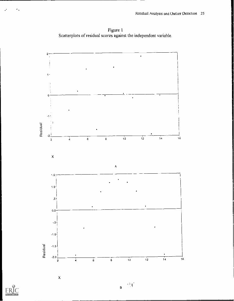
The following discussion is based in large part on the four scatter plots presented in Figure 1

These concepts were first illustrated by Anscombe (1973) in a seminal paper exploring the use of

uaphs in statistical ana;ysis. Similar scatter plots have since been used in many text books on

regression analysis to elegantly illustrate how a graphical analysis of residual scores can uncover

hidden structures in the data that violate the least squares regression model (see Chatterjee &

Price. 1991. Glantz & Slinker, 1990; Hamilton, 1990., Pedhazur. 1993)

INSERT FIGURE 1 ABOUT HERE

The scatter plots in Figure I were created by plotting the residual e scores on the ordinate

against the independent variable X values on the abscissas for fictitious data sets As

demonst .ated by Anscombe (1973), data sets fi.)r all four graphs in Figure 1 can be created that

Residual Analysis and Out !kr Detection 5

yield equivalent statistics through regression analysis. That is, data sets represented by these four

graphs can be created that produce identical regression coefficients, equations for regression lines,

regression sum of squares, residual sum of squares, and multiple R2. If all the observations are

considered to be reliable without evidence of some gross recording error then the statistics would

lead to similar interpretations, yet the data are remarkably different. This information would be

undeeted if such scatterplots were not examined

If the assumptions underlying regression analysis hold, then the residual e scores will be

normally distributed about a mean of zero with constant variance throughout the line originating

throughthe mean of the residuals. In plainer language this can be stated as the e scores falling

along a constant width band centered on zero in the residual graph. Figure I A illustrates such a

plot That is, the residuals are reasonably randomly scattered about zero with constant variance

regardless of the value of the independent variable, X. Further, none of the residuals is notably

large in either the positive or negative direction, suggesting that there are no extreme "outlier"

data points that disproportionally bia the linear regression equation (the concept of outliers will

be more thoroughly discussed later in the paper). If the linear regression model was misspecified

(meaning that the aforementioned underlying assumptions were violated), then the residuals

would deviate from the expected pattern about zero. Trends up or down , curves, or a

"megaphone" shape with one end of the band narrower than another in the residual plot would

indicate violations of the homoscedasticity and.'or linearity assumptions.

Figures I B, C. and D represent residual patterns that call into question the validity of the

regression analysis In Figure 1B the pattern obviously violates the assumption that the variables

are related linearly Rather, there appears to he a curvilinear relationship with negative residuals

concentrated at low and high values of X and positive residuals concentrated at intermediate

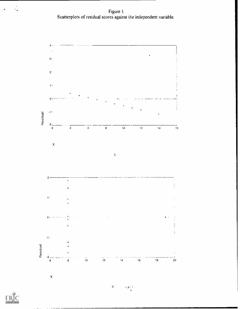
Residual Analysis and Outlier Detection

values of X A quadratic rather than a linear equation would do a better job of describing the

relationship between variables in this case. Barringer (1995) explains the procedures for analyzing

such data What is most notable about Figure IC is the outlying data point associated with a large

residual value. This particular outlier is known as an outlier in the Y direction and will greatly

influence the slope and intercept ot the regression equation. This is particularly true in view of

the fact that all of the residuals accept the outlier are systematically (not randomly) scattered

about zero with positive residuals at low values of X and negative residr-ls at high values of X

Figure ID denotes another outlying data point the exerts great influence on the regression

equation However, in this case the data point is an outlier in the x direction and does not possess

a large residual score (in fact, the residual score is 0). These data violate the assumption of

homoscedasticitv as they do not vary constantly about the line e = 0 and call into to question the

normality of the X variable. Further, the data set is simply unsuitable for linear fitting as the

regression line is determined essentially by only one data point Moreover, if' the outlier were to

be dropped from the analysis, the regression relation would be near zero. This can be more

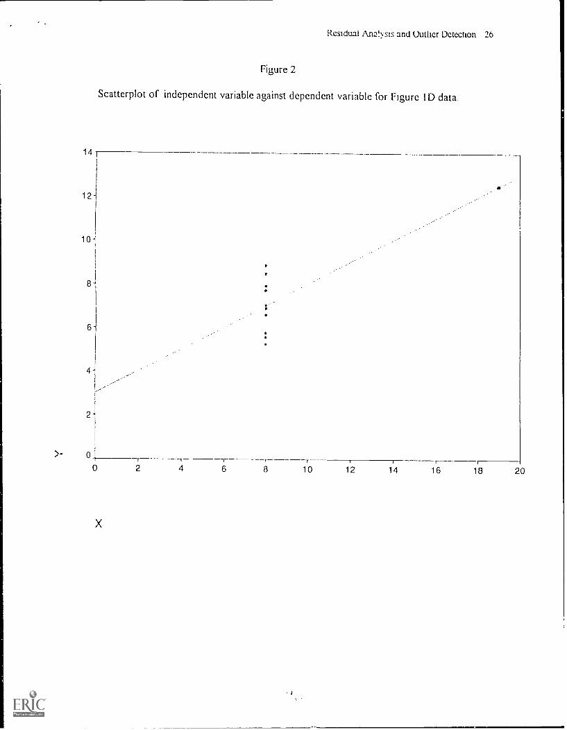
readily seen by examining a simple scatter plot of the dependent Y variable against the

independent X variable for this data, as seen in Figure 2. If the data point to the far right AN ere

deleted or moved in any direction the regression equation would correspondingly being adjusted

as the regression line would be tilted As stated by Anscombe (1973), "We are usually happier

about asserting a regression relation if the relation is still apparent after a few observations (any

ones) have been deleted - that is, we are happier if the regression relation seems to permeate all

the observations and does not derive largely from one or two- (p 19)

INSERT FIGLIRE 2 ABOUT HERE


In the case of multiple independent variables, residuals can be plotted against each

independent variable and examined for model violations, as shown above. Thus, providing two

dimensional graphs which are more easily comprehended at a glance than multidimensional graphs

involving pianes. Further, residuals can be plotted against the fitted Yhat values in either bivariate

or multivariate regression. By standardizing the e and the Yhat scores so that the scales for both

axis are the same in this plot, one can at a glance observe the relative dispersions of the fitted

values and the residual scores. The researcher will obviously hope that the Ynat scores are near

the observed Y scores so that the variability of the Yhat is greater than that of the residual e

scores. This discussion is not an exhaustive listing of the variety of ways that scatter plots can be

used in data analysis. It is hoped that this brief examination of the topic provides support for the

common recommendation found in many statistical texts: examine ihe plotted data.

Four Quantitative Approaches to Residual Analysis and Outlier Detection

Four commonly used quantitative approaches to outlier detection are briefly reviewed and then

used to examine fictitious data sets. The four methods are: standardized residuals, Leverage,

studentized residuals, and Cook's distance As alluded to above, outliers are data points that fall

a considerable distance away from the majority of the other data. Outliers can be thought of as

falling along two scales, namely along the X and Y scales. Further, there can be outliers in

varying degree in both directions. An outlier in the Y direction will have a large residual e score

associated with it and can potentially influence the regression parameters (i.e., slope and intercept)

by "pulling" the regression line towards the score's Cartesian coordinate so as to minimize the

residual e scores. An outlier in the X direction can also greatly influence the regression

parameters, however, it's residual score may be small as demonstrated in Figure I D Outliers in

the direction of the independent variable are by no means uncommon, particularly in the social

Residual Analysis and Outher Detection 8

sciences where the independent X variables are observed quantities subject to random variability.

In fact, having outliers in relation to the independent vari..ales is probably more likely when there

is only one dependent variable and multiple independent variables, thus providing more

opportunity for things to go wrong (Rousseeuw & Leroy, 1987).

Standardized Residuals: The standardized residual is one method of identif'ying outliers in the

Y direction. If a regression analysis were carried out on the data represented in Figure IC after

deleting the outlier, considerably different regression parameters (e.g., R and weights) would

be calculated. Such an outlier is said to have "influence" on the regression equation and can be

identified by examining standardized residuals. As defined earlier, raw e scores are calculated as:

ei = Yi - Yhati

Standardized residuals are derived by dividing the raw e scores by the standard deviation of the

residual scores, also referred to as the standard error of estimate. The standard error of estimate

can be thought of as an estimate of the standard deviation of the population about the line (or

plane) of means. Thus the standardized residual is calculated by

es = e

where es is the standardized residual, e is the raw residual, and s is the standard deviation of

the residual scores. Because e and s are in the same units, es is unitless and does not depend

on the scale of measurement used to quantify the dependent variable Y. The advantage of this is

that now general rules of thumb can be established for how far away a data point must lie before it

is identified as an outlier. A standardized residual score of 0 means that a data point falls on the

regression line. Further, a standardized residual of I means the point falls 1 standard deviation

from the regression plane or line. Likewise, a standard residual of 2 indicates that the data point

is 2 standard deviations away and so on


As noted earlier, one of the assumptions of regression analysis is that the population members

are normally distributed about the plane of means. Hence, the residuals are normally distributed

about the regression line or plane. Normal distributionby definition means that about two thirds

of the data points fall withm 1 standard deviation of the of the regression line and approximately

95% fall within 2 standard deviations. Moreover, one would expect about 66% of the

standardized residuals to have absolute values below 1 and almost all of the standardized residuals

to have absolute values below 2. A general rule of thumb then is to identify data points with

standardized residuals of 2 or more as potential outliers. These are thought to be outliers that

can potentially have great influence on the regression parameters.

Two caveats should be observed when analyzing standardized residual scores. First, a

standardized residual does not mean a data point is necessarily a mistake in recording or a special

outlying observation for which the hypothesis being studied does not hold In all normal

populations, about 5% of the members exceed 2 standard deviations from the mean. Therefore,

the above rule of thumb should not be used rotely. Second, an analysis of standardized residual

scores will not identify outliers in the X direction. The outlier in Figure ID, as noted previously,

has a residual score of 0 (hence, a standard residual score of 0) and would be missed by solely an

analysis of the standardized residuals.

Leverage: A point that is an outlier in the x direction is called a potential leverage point.

Because a leverage point falls far away from the center of the independent variable values it can

exert great influence on the regression equation as seen in Figure 2 It would be helpful then to

quantify the leverage value of any particular data point in order to identify such an influential

point Such quantity in the case of one independent variable is given by the equation

h, = 1/n + (X, X)2/ E (X, - X)2


where 111 is a measure of how much the observed value of the dependent variable affects the

estimated Yhat value for the ith data point. In other words 111 is a measure of the relationship

that transforms the observed Y, values to the predicted Yhat, values for each individual data

point. This transformation is analogous to the slope and intercept parameters used in regression

that transform Y to Yhat, however, these parameters are constants while 11, varies from point to

point Thus hi can be used to diagnose individual data points that potentially are influential

leverage points. Note that hi depends only on sample size and the values of the independent

variables. As the X, values move farther away from the mean of the independent X values, the

leverage increases. Hence, leverage is focused on identifying outliers in the x direction.

It would be desirable that all the points have the same influence on the predicted Yhat values

so that all the leverage values would be equal and small. Moreover, if all the data points are

contributing equally to the regression equation then a stronger case can be made for the predicted

linear relationship. It can be shown that leverage values fall between 0 and I (Belsley & Welsch.

1980). It can also be shown that the expected (average) value of leverage is

expected 11, = (k + 1)/n

where k is the number of independent variables in the regression analysis It has been suggested

that the cut off point for identifying a potential leverage point is twice the expected h,

(Rousseeuw & Leroy,1987). Therefore, when hi> 2(k + 1)/n fbr the point in question, it's

designated as having high leverage and warrants fin-ther investigation. However, just because a

data point has a high ff, value does not mean the point is necessarily exerting disproportional

influence on the regression equation For example, an outlier in the x direction may be identified

while the regression analysis with or with out the identified point generates similar results. This

may happen where a cluster of data points produces a regression line that also runs through the

Residual Analysis and Outlier Detection I I

outlying point Such a point strengthens our confidence in the regression equation bv suggesting

that a linear relatioship holds true for extremely low or high values of the independent variable.

Studentized Residuals: Standardized residual are normalized by dividing e by the standard error

of measurement, s . If the data fit the assumptions underlying regression then ss , will be

constant for all values of the independent variable, X. However, data points that lie further away

from the "center" (center being defined by the mean of X and the mean of Y) of the data will

obviously have areater error of measurement associated with them. Hence, one can be more

confident about the location of the regression line for those points that cluster around th.; "center"

of the data It is possible then to take this effect into account when normalizing the residuals and

increase the sensitivity of the residuals to outliers. This is accomplished by dividing each es value

-/ its specific standard error, which is a function of how far X is from the mean of X. As noted

earlier, this distance can be quantified by the leverage calculation The equation for the

studentized residual is

r, e, / , Jl - h,

The studentized residual is more sensitive to outliers than is the standardized residual because

it is sensitive to outliers in both the Y and to some degree in the X direction. As can be seen in

the equation, larger ri values will be created by not only higher magnitudes of the e scores but

also by higher magnitudes of leverage quantities

The above equation represents what is typically referred to as the internally studentized

residual because the estimate of s is computed by using all the data An alternate calculation

can be done by computing the standard deviation error after deleting the data point in question.

This is typically referred to as the externally studentized residual The reasoning is that robust

regression results would not be effected by deleting one point Utile point is in fact an outlier


then the estimation of s would be inflated and s ..erstate the magnitude of the outlier effect

as a appears in the denominator of the equation Removing the data point in question from the

analysis makes the externally studentized residual more sensitive to outliers Similar cut off points

arc recommended for identification of outliers for this technique as were recommended for the

standardized residuals (i.e., studeotized scores of 2 or more). However, instead of rotely applying

the cu,.!,:ff points, it is more informative to look at the relative differences among the scores

Cook's Distance: So far the techniques reviewed have been directed at identifying "potential-

influential outliers. The basic logic utilized by these techniques is that the further a point falls

away from the center of the data, the higher the probability is that the point will influence the

regression equation. Howeveris was mentioned in regards to leverage, a point can be identified

by these techniques and not necessarily be disproportionally influential in regression analysis A

technique that more directly measures the actual influence of a data point is Cook's distance This

is accomplished by computing how much the regression coefficients change when the point in

question is deleted Cook's distance is given by

CD, = k -*-11(h,/ 1 hi)

CD, can be thought of as a distance between one set of regission coefficients obtained by

deleting the ith data point and the other set of regression coefficients obtained by using the whole

data set One way to think of this distance is to plot the coefficients against eachother and then

measure the distance between the two points that the coefficients generate Therefore, when CD,

is a large number, the ith data point is having a major effect on the regression coefficients

Judging from the equation it follows that CD, depends on three quantities First, CD, is

effected by the number of independent variables, k That is, as the number of independent

variables increases (other things being held constant) CD, decreases Second, CD, is determined

,


by the internally studentized residual, which is primarily a measure of the point's relative distance

from the center of the data in the y direction Third, CD; is adjusted by the leverage of the ith

data point, which is a measure of the point's relative distance from the center of the data in the x

direction. Hence, a large value of CD; could be a result of the data point having a large

studentized residual , or a large leverage, or both. CD; values exceeding I are considered to be

worth further investigation while values exceeding 4 are considered serious outliers (Fox, 1984).

Concrete Examples of Outlier Detection Using Fictitious Data Sets

Four data sets were analyzed using SPSS/PC. The first data set consisted of 12 pairs of X

and Y values The other three sets were created by simply adding one additional data point to the

first data set so that n = 13 The added point was varied in terms of its "outlyingness" in either

the x or y directions. Outlier detection methods of standardized residuals, leverage, externally

studentized residuals, and Cook's distance were carried out for each data set. Table I lists the

regression statistics generated by each data set and Tables 2 through 5 contain the computed

values for the various detection techniques

INSFRT TAM P 1 ARCM IT 1-1FRF

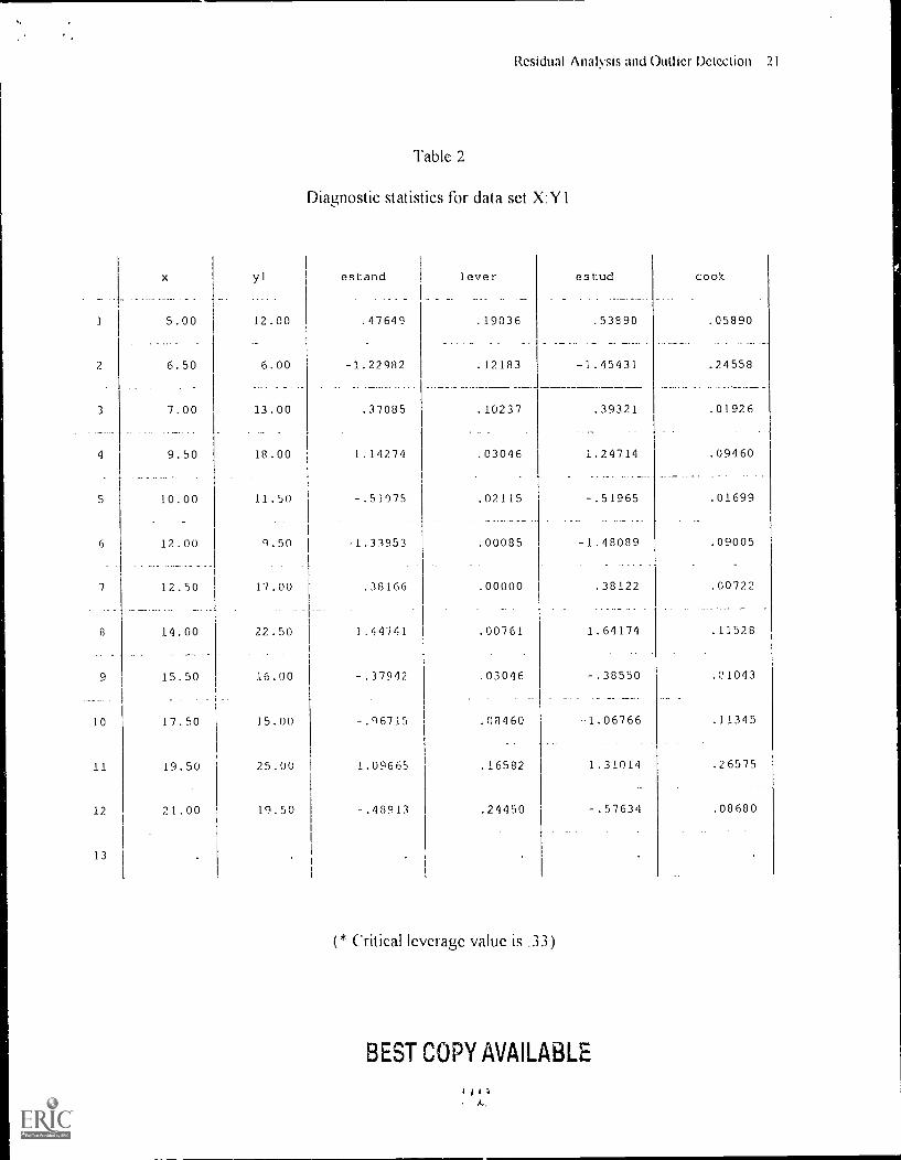
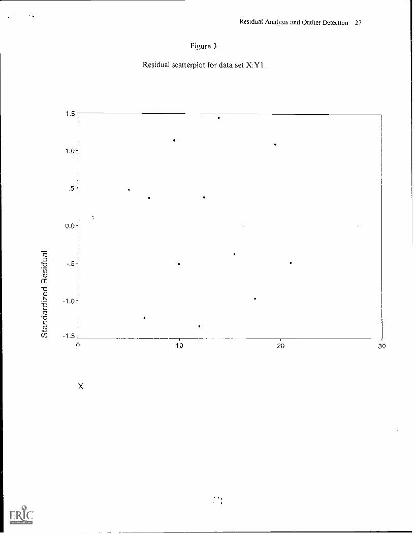
The data set represented in the residual scattergram in Figure 3 and in Table 2 was created to

illustrate a least squares linear regression analysis in which the underlying assumptions of

regression are met and no outliers are detected. Furthct, as noted in Table I this data set

(i e , X Y1) generated a multiple R of .68, suggesting a fairly good fit to the linear relationship

outlined by the regression parameters

INSURT F1(AIRF AI-101_1T 1-1PRF


As can been seen in Figure 1 the residuals appear to be normally distributed about a mean of 0

and their spread about the line e = 0 for all values of X appears to be consistent. That is, the

residual scores appear to be homoscedastic. Further, none of the diagnostic quantities reveal the

presence of an outlier. None of the standardized or studentized residuals are above 2, none of the

leverage values exceed the critical value of .33, and none of the CD; values are above 1. Hence,

the regression equation for this data set appears to describe the relationship between the variables

well.

INSFRT TAR! F 7 AROLIT HFRF

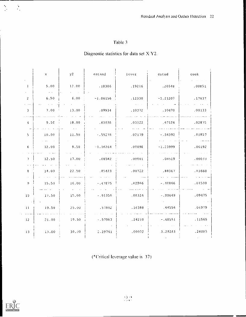
To create the X Y2 data set a thirteenth data point was added that represented an outlier in y

direction. As can be seen in Table 1, multiple R went from .68 to .57, suggesting that the data

point is quite influential in the regression analysis. Notably the slope parameter did not change

much while the intercept moved upward approximately 1.2 units. This is to be expected as the

outlier is towards the center of the X values but lies considerably higher than the center of the Y

values. Thus, the line would not be -leveraged" or tilted, but rather, is pulled upward relatively

evenly towards the outlier. As can be seen in Table 3, the data point is identified as an outlier

only by the standardized and studentized residual. Further, the rclative value of the two residual

scores illustrates that the studentized residual tends to be more sensitive to outliers in the y

direction. Moreover, the studentized residual score of 3.3 marks this point as an extreme outlier

while the standarized residual score of 2.29 flags the point as a moderate outlier

INISFRT TART F ARCM IT HFRF

t


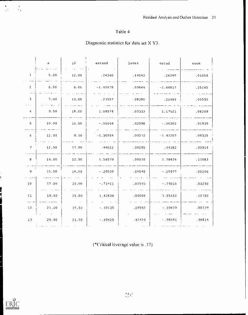
The additional data point added to data set X:Y3 is an outlier chiefly in the x direction.

Table 4 shows that the only diagnostic value that detects data point 13 as an outlier is the leverage

value (i.e., hi exceeds the critical value of .37). Although the point falls a considerable distance

away from the center of the X data, it does not appear to substantially effect the regression

analysis. In fact, the multiple R remains virtually unchanged, as noted in Table I. The addition

of this rilata point then strengthens our confidence in the linear relationship outlined by the

regression analysis. This data set is a good example of a data point being flagged as a leverage

point but not as an influential outlier. Had the point fallen further off the initial regression line

(i e , prior to adding point 13), in either the negative or positive direction in terms of Y. the

regression equation could have been greatly effected.

INSFRI TART F 4 AROUT HFRF

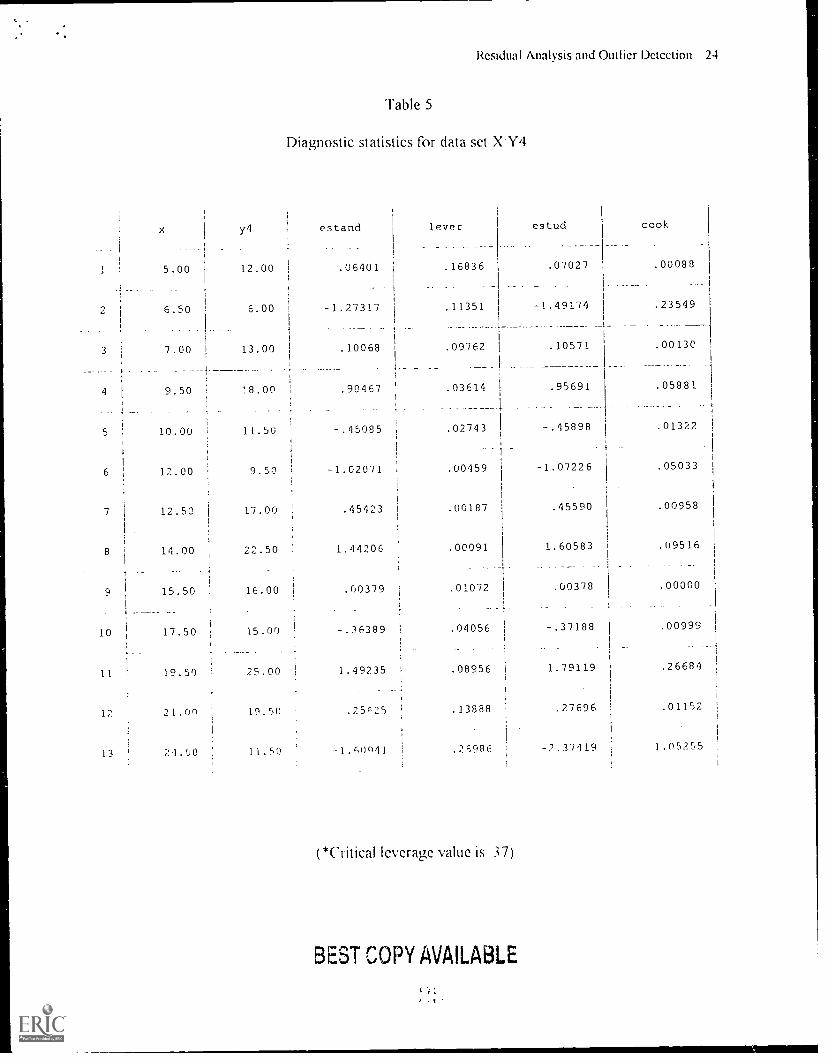
The final data set X Y4 was created by adding a data point that was an outlier in both

directions. As can be seen in Table 1, the regression statistics were all greatly effected by the

addition of this one point. Most notably, multiple R went from .69 to .45, considerably lowering

our confidence in the fit of the regression line to the data. Data point 13 was flagged as an outlier

by the studentized residual score of -2 4 and a Cook's distance value of 1.05. This underscores

the point that if only sta:dardized residuals and leverage vvere used this information would be

missed In fact, in none of the data sets did all four techniques pick up the same point. These

data sets have illustrated the need for multiple approaches when attempting to identify influential

data points as one approach is not capable of flagging all types of potential outliers

BEST COPY AVAILABLE


INISFRT TARI F: S AFflI IT HFRF

Conclusions

A final note should be made regarding the examples given so far. Data sets

presented in this paper are small and contain only one independent and dependent variable. Both

these aspects greatly simplify the processes of identifying influential outliers. As more variables

are added, multiple dimensions are also added to the data picture. It becomes increasingly

difficult to interpret data in multiple dimensions, and so, it becomes increasingly difficult to define

influential points in the regression analysis as more and more variables are added Additionally,

the techniques illustrated are more likely to be helpful when there are only one or two outliers.

However, it is quite possible that a group cf points is exerting influence thus requiring more

complicated computations and, at times, different techniques for detection For example, when

attempting to detect multiple outliers by looking at the effect of deleting one point at a time, the

number of all possible subsets might be gigantic leading to extensive computations.

The present paper has outlined several techniques for detecting outliers. The underlying

premise for using these techniques is that the researcher needs to make sure conclusions based on

the data are not solely dependent on one or two extreme observations. If no outliers are

detected, then obviously confidence in the findings is bolstered. However, once an outlier is

detected the researcher must examine the data point's source of aberration. Outliers can be

present in a sample because of errors in recording observations and/or errors in transcription (i.e ,

measurement error). If this is the case then deleting the observation from the data set is

defensible. However, outliers may also be present due to an exceptional occurrence in the

investigated phenomenon. Moreover, such an occurrence suggests that the model (i.e., in this


case the least squares regression model) does not adequately describe the relationships among the

variables. Only through careful study of the data and the literature can decisions be made as to

how to proceed with the analysis when a model violation has occurred Therefore, outlier

detection methods are useful but no substitute for a sound understanding of the phenomenon

being studied

Residual Analysis and Outlier Detection i 8

References

Anscombe, F.J. (1973). Graphs in statistical analysis American Statistician, 27, 17-21.

Barringer, M.S (1995, April). Curvilinear relationships in special education research: How

multiple regression analysis can be used to investigate nonlinear effects. Paper presented at

the annual meeting of the American Educational Research Association, San Francisco.

(ERIC Document Reproduction Service No. ED 382 641)

Belsey, P A. & Welsch, R.E. (1980). Regression diagnostics: Identifying influential data and

sources of collinearitv. New York: Wiley.

Bohrnstedt, G.W. & Carte, T.M (1971). Robustness in regression analysis. In H.L. Costner

(Ed.) Sociological methodology (pp 113-132). San Francisco, CA: Jossey-Bass.

Chatterjee, S. & Price, B. (1991). Regression analysis by example (2nd ed ). New York:

Wiley.

Fox, J (1984). Linear statistical models and related methods: With applications to social

research New York: Wiley.

Glantz, A.G. & Slinker, B.K. (1982). Primer of applied regression and analysis of variance. San

Francisco, CA: Holt, Rinehart, and Winston.

Glass, G V. & Hopkins, K D. (1984). Statistical methods in education and psycholou (2nd

ed ) New Jersey: Prentice Hall.

Hamilton, C.C. (1990). Modern analysis. A first course in applied statistics. Pacific Grove,

CA. Brooks/Cole

Hecht, J.B. (1991, April). Least-Squares linear regression and Schrodinger's cat: Perspectives

on the analysis of regression residuals. Paper presented at the annual meeting of the

- a.


American Educational Association, Chicago. (ERIC Document Reproduction Service No. ED

333 020)

Hecht, J.B. (1992, April). Continuing perspectives on the analysis of regression residuals:

Advocacy for the use of a "Totter Index." Paper presented at the annual meeting of the

American Educational Association, San Francisco. (ERIC Document Reproduction Service

No. ED 347 194)

Keppel, G. & Soufley, W H (1980) Introduction to design and analysis New York: Freeman

and Company.

Pedhazur, E J. (1982). Multiple regression in behavioral research Expiniation and prediction

(2nd ed.). New York. Holt, Rinehart, and Winston.

Rousseeuw, P J. & Leroy, A.M. (1987). Robust regression and outlier detection. New YorkWiley.


Table 1

Regression statistics generated by each heuristic data set

Statistics

Multiple R

X.Y1

ng

l1

i

I

X.Y2 1

57

X.Y3

69

X.Y4

45

1 R squared 47 3 i .47 .20

b

pararn,, ,77 1 74 55 41

a

linterreptparaITICtCr)

6.43 I 7.24 8.20 I 9 64

1

2

3

4

5

6

7

8

9

10

11

12

13


Table 2

Diagnostic statistics for data set KNI

xi

ylI

estand lever estud cook

5.00 12.00 .47649 .19036 .53890 .05890

6.50 6.00 -1.22982 .12183 -1.45431 .24558

7.00 13.00 .37085 .10237 .39321 .01926

9.50 18.00 1.14274 .03016 1.21714 .09460

10.00 11.50 -.51075 .02115 -.51965 .01699

12.00 9.50 -1.33953 .00085 -1.18089 .09005

12.50 17.00 .38166 .00000 .38122 .00722

14.00 22.50 1.14741 .00761 1.64174 .11528

15.50 16.00 -.37942 .03046 -.38550 .01043

17.50 15.00 -.96715 .08460 -1.06766 .11345

19.50 25.00 1.09665 .16582 1.31014 .26575

21.00 19.50 -.48913 .24450 -.57634 .08680

(* Critical leverage value is .33)

BEST COPY AVAILABLE

A.


Table 3

Diagnostic statistics for data set X:Y2.

y2 estand lever estud cook

1 5.00 12.00 .18386 .19216 .20548 .00851

2 6.50 6.00 -1.06156 .12330 -1.21207 .17637

3 7.00 13.00 .09934 .10372 .10470 .00133

4 9.50 18.00 .65038 .03122 .67126 .02875

_--5 10.00 11.50 -.55278 .02179 -.56392 .01857

--6 12.00 9.50

I-1.16264 .00098 -1.23999 .06192

7 12.50 17.00 .08582 .00001 .08519 .00033

8 11.00 22.50 .85423 .00722 .88367 .03660

:

q t 15.50 16.00 -.17875 .02966 -.48866 .01530

10 17.50 15.00 ; -.91350 .08324 -.99649 .09475

11 I 19.50 25.00 .57802 .16388 .64556 .06979

12 21.00 19.50 -.57983 .24210 -.68551 .11565

13 13.00 30.00 2.29741 .00072 3.29203 .24085

(*('ritical leverage value is 37)

Residual Analsis and Outlier Detection 23

Table 4

Diagnostic statistics for data set XY3.

x y3 estand lever estud cook

1 5.00 12.00 .24360 .14063 .26349 .01054

2 6.50 6.00 -1.40679 .09664 -1.66817 .25145

3 7.00 13.00 .21557 .08380 .22193 .00530

4 9.50 18.00 1.08574 .03333 1.17021 .08209

5 10.00 11.50 -.55064 .02598 -.56303 .01939

_ -- --6 12.00 9.50 '-1.30281 .00572 -1.42207 .08335

7 12.50 17.00 .44022 .00295 .44182 .00914

8 14.00 22.50 1.56579 .00010 1.78426 .11083

9 15.50 16.00 -.20530 .00548 -.20477 .00206

10 17.50 15.00 -.71611 .02515 -.74015 .03258

11 19.50 25.00 1.42836 .06006 1.65452 .18762

12 21.00 19.50 -.10135 .09562 -.10629 .00129

13 29.00 21.50 -.69625 .42424 -.98441 .48816

(*Critical leverage value is .37)


Table 5

Diagnostic statistics for data set X-Y4

Y4 estand lever estud cook

_

1 5.00j

12.00 .06401 .16836 .07027 1 .00088

2 6.50 6.00 -1.27317 .11351 -1.49174 .23549

3 7.00 I 13.00 .10068 .09762 .10571 .00130

. _

--------

4 I 9.50 18.00 1 .90467 .03614 .95691 .05881

------.5 10.00 11.50 -.45085 .02743 -.45898 .01322

6 12.00 9.50 ; -1.02071 .00459 -1.07226 .05033

1

7 12.50 1 17.00 .45423 .00187 .45590 .00958

1

8 14.00 22.50 : 1.44206 .00091 1.60583 .09516

15.50 : 16.00 .00379 .01072 .00378 .00000

10 17.50 15.00 1 -.36389 .04056 -.37188 .00999

_

11 19.50 25.001 1.49235 .08956 1.79119 .26684

12 21.00 19.50 : .25r25 .13888 27696 .01152

. .

13 21.00 1 11.50 -1.r0941 .26986 -7.37119 1.05255

(*Critical leverage value is 37)

BEST COPY AVAILABLE


Figure 1Scatterplots of residual scores against the independent variable.

0

4 6 8 10 12 14 16

A

1.5

51

0.0

-1 OJ

TO -1 .5 17P

I6a) I

cc -2.0

2 4 6 8 10 12 14 16

4

Figure 1Scatterplots of residual scores against the independent variable.

3-

2-

2

2 4 6 8 10 12 14 16

4

6 8 10 12 14 16 18 20

14

Residual Ana!ysis and Outlier Detection 26

Figure 2

Scatterplot of independent variable against dependent variable for Figure ID data.

121

10,

0

X

--r2 4 6 8 10 12 14 16 18

1.5


Figure 3

Residual scatterplot for data set X Y1

.5 .

0.0.

-1.50 10 20

Documents

DOCUMENT RESUME ED 395 949 TM 025 016 … the assumptions underlying regression analysis hold, then the residual e scores will be normally distributed about a mean of zero with constant