Embed Size (px)
Citation preview

2016-ENST-0043
EDITE - ED 130
Doctorat ParisTechT H È S E
pour obtenir le grade de docteur délivré par
TELECOM ParisTechSpécialité « INFORMATIQUE et RESEAUX »
présentée et soutenue publiquement parDuy-Hung PHAN
le 18 julliet 2016
E�cient and Scalable Aggregationfor Data-Intensive Applications
Directeur de thèse: Professeur Pietro MICHIARDI
JuryMme. Elena BARALIS, Professeure, Politecnico di Torino Rapporteuse
M. Guillaume URVOY-KELLER, Professeur, Université Nice Sophia Antipolis (UNS) Rapporteur
M. Bernard MERIALDO, Professeur, Département Data Science, EURECOM Examinateur
M. Fabrice HUET, Chargé de Recherche HDR, INRIA Sophia Antipolis Examinateur
TELECOM ParisTechécole de l’Institut Télécom - membre de ParisTech

Abstract
The past decade has witnessed the era of big-data. Due to the vast volume of data, tra-
ditional databases and data warehouses are facing problems of scalability and e�ciency.
As a consequence, modern data management systems that can scale to thousands of
nodes, such as Apache Hadoop and Apache Spark, have emerged and quickly become
the de-facto platforms to process data at massive scales.
In these large-scale systems, many data processing optimizations that were well studied
in the database domain have now become futile because of the novel architectures and
distinct programming models. In this context, this dissertation pledged to optimize one
of the most predominant operations in data processing: data aggregation for such large-
scale data-intensive systems.
Our main contributions were the logical and physical optimizations for large-scale data
aggregation, including several algorithms and techniques. These optimizations are so
intimately related that without one or the other, the data aggregation optimization prob-
lem would not be solved entirely. Moreover, we integrated these optimizations as essen-
tial components in our multi-query optimization engine, which is totally transparent to
users. The engine, the logical and the physical optimizations proposed in this disserta-
tion formed a complete package that is runnable and ready to answer data aggregation
queries from users at massive scales. To the best of our knowledge, this dissertation is
among the foremost to provide a complete and comprehensive solution to execute ef-
�cient and scalable data aggregation queries for large-scale data-intensive applications
using MapReduce-like systems.
Our optimization algorithms and techniques were evaluated both theoretically and ex-
perimentally. The theoretical analyses showed the reasons why our algorithms and tech-
niques are a lot more scalable and e�cient than other state of the art works. The exper-
imental results using a real cluster with synthetic and real datasets con�rmed our anal-
yses, showed a signi�cant performance improvement and revealed various angles about
our algorithms. Last but not least, our works are published as open source softwares for
public usages and studies.
3


Acknowledgements
I would not be able to go this far in my PhD journey if not for my advisor, Prof. Pietro
Michiardi. I am extremely thankful for his immense support and guidance. I learned
many lessons from him, not only in academia but also in daily life. Working with him is
a joy because of his knowledge, his experience and most important, his enthusiasm. To
be fair, he is always able to push me one step forward, which I ultimately realize that it
helped me to build up and broaden my mindset. So again, I am thankful to be his student,
and I hope that in future, we would have chances to work together.
There are also other people that directly contributed to my works. My special thanks go
to Matteo Dell’Amico for his advices and discussion, to Quang-Nhat Hoang-Xuan for his
huge assistance in implementing and maintaining our open source softwares, to Daniele
Venzano for his support on setting up our cluster.
Even more fortunately, I have been a member of a fantastic group, the Eurecom Dis-
tributed System Group, where I have learned, grown and developed as a researcher and
an engineer. Thank you Xiaolan Sha, Mario Pastorelli, Antonio Barbuzzi, Duc-Trung
Nguyen, Francesco Pace and Trong-Khoa Nguyen for making my journey full of friend-
ship and support.
I would like to dedicate this dissertation to my parents, my sister and my �ancée, Vy,
who have loved and supported me unconditionally. I love you with all my heart.
5


Table of Contents
Table of Contents 7
1 Introduction 151.1 Contributions and Dissertation Plan . . . . . . . . . . . . . . . . . . . . . 16
1.1.1 Logical Optimization for Data Aggregation . . . . . . . . . . . . 17
1.1.2 Physical Optimization for Data Aggregation . . . . . . . . . . . . 18
1.1.3 Multi-Query Optimization Engine . . . . . . . . . . . . . . . . . 18
1.1.4 Dissertation Plan . . . . . . . . . . . . . . . . . . . . . . . . . . . 19
2 Background 212.1 Data Aggregation . . . . . . . . . . . . . . . . . . . . . . . . . . . . . . . 21
2.2 Large-Scale Data Processing Model . . . . . . . . . . . . . . . . . . . . . 22
2.2.1 MapReduce Model Fundamentals . . . . . . . . . . . . . . . . . . 23
2.2.2 Resilient Distributed Datasets Fundamentals . . . . . . . . . . . . 23
2.2.3 Discussion of Our Choices . . . . . . . . . . . . . . . . . . . . . . 25
2.3 Execution Engines, High-level Languages and Query Optimization . . . 26
2.3.1 Execution Engines . . . . . . . . . . . . . . . . . . . . . . . . . . 26
2.3.2 High-level Languages . . . . . . . . . . . . . . . . . . . . . . . . 26
2.3.3 Query Optimization . . . . . . . . . . . . . . . . . . . . . . . . . 27
2.4 Summary . . . . . . . . . . . . . . . . . . . . . . . . . . . . . . . . . . . . 28
3 Logical Optimization for Large-Scale Data Aggregation 293.1 Introduction . . . . . . . . . . . . . . . . . . . . . . . . . . . . . . . . . . 29
3.2 Problem Statement . . . . . . . . . . . . . . . . . . . . . . . . . . . . . . 30
3.2.1 De�nitions . . . . . . . . . . . . . . . . . . . . . . . . . . . . . . 31
3.2.1.1 Search DAG . . . . . . . . . . . . . . . . . . . . . . . . 31
3.2.1.2 Problem Statement . . . . . . . . . . . . . . . . . . . . 33
3.2.2 Cost model . . . . . . . . . . . . . . . . . . . . . . . . . . . . . . 34
3.3 Related Work . . . . . . . . . . . . . . . . . . . . . . . . . . . . . . . . . . 35
3.4 The Top-Down Splitting Algorithm . . . . . . . . . . . . . . . . . . . . . 37
3.4.1 Top-Down Splitting algorithm . . . . . . . . . . . . . . . . . . . . 37
3.4.1.1 Constructing the preliminary solution tree . . . . . . . 37
7

8 TABLE OF CONTENTS
3.4.1.2 Optimizing the solution tree . . . . . . . . . . . . . . . 38
3.4.2 Complexity of our algorithm . . . . . . . . . . . . . . . . . . . . 40
3.4.2.1 The worst case scenario . . . . . . . . . . . . . . . . . 41
3.4.2.2 The best case scenario . . . . . . . . . . . . . . . . . . 42
3.4.3 Choosing appropriate values of k . . . . . . . . . . . . . . . . . . 43
3.5 Experiments and Evaluation . . . . . . . . . . . . . . . . . . . . . . . . . 45
3.5.1 Experiment Setup . . . . . . . . . . . . . . . . . . . . . . . . . . . 45
3.5.2 Cost model in our experiments . . . . . . . . . . . . . . . . . . . 46
3.5.3 Scaling with the number of attributes . . . . . . . . . . . . . . . . 46
3.5.4 Scaling with the number of queries . . . . . . . . . . . . . . . . . 48
3.5.5 Scaling with both number of queries and attributes . . . . . . . . 50
3.5.6 The impact of cardinality skew . . . . . . . . . . . . . . . . . . . 52
3.5.7 Quality of solution trees . . . . . . . . . . . . . . . . . . . . . . . 52
3.6 Discussions and Extensions . . . . . . . . . . . . . . . . . . . . . . . . . . 54
3.6.1 Intuition and Discussion . . . . . . . . . . . . . . . . . . . . . . . 54
3.6.2 Di�erent Aggregate Functions . . . . . . . . . . . . . . . . . . . . 55
3.7 Summary . . . . . . . . . . . . . . . . . . . . . . . . . . . . . . . . . . . . 56
4 Physical Optimization for Data Aggregation 594.1 Design Space of MapReduce-like Rollup Data Aggregates . . . . . . . . . 59
4.1.1 Introduction . . . . . . . . . . . . . . . . . . . . . . . . . . . . . . 59
4.1.2 Background and Related Work . . . . . . . . . . . . . . . . . . . 61
4.1.3 Problem Statement . . . . . . . . . . . . . . . . . . . . . . . . . . 62
4.1.4 The design space . . . . . . . . . . . . . . . . . . . . . . . . . . . 64
4.1.4.1 Bounds on Replication and Parallelism . . . . . . . . . 64
4.1.4.2 Baseline algorithms . . . . . . . . . . . . . . . . . . . . 66
4.1.4.3 Alternative hybrid algorithms . . . . . . . . . . . . . . 72
4.1.5 Experimental Evaluation . . . . . . . . . . . . . . . . . . . . . . . 74
4.1.5.1 Experimental Setup . . . . . . . . . . . . . . . . . . . . 74
4.1.5.2 Results . . . . . . . . . . . . . . . . . . . . . . . . . . . 74
4.2 E�cient and Self-Balanced Rollup Operator for MapReduce-like Systems 79
4.2.1 Introduction . . . . . . . . . . . . . . . . . . . . . . . . . . . . . . 79
4.2.2 Preliminaries & Related Work . . . . . . . . . . . . . . . . . . . . 80
4.2.2.1 Rollup in Parallel Databases . . . . . . . . . . . . . . . 80
4.2.2.2 Rollup in MapReduce . . . . . . . . . . . . . . . . . . . 81
4.2.2.3 Other Related Works . . . . . . . . . . . . . . . . . . . 82
4.2.3 A New Rollup Operator . . . . . . . . . . . . . . . . . . . . . . . 83
4.2.3.1 Rollup Operator Design . . . . . . . . . . . . . . . . . . 83
4.2.3.2 The Rollup Query: Algorithmic Choice . . . . . . . . . 85
4.2.3.3 The Tuning Job . . . . . . . . . . . . . . . . . . . . . . 86
4.2.3.3.1 Balancing Reducer Load . . . . . . . . . . . . 86

TABLE OF CONTENTS 9
4.2.3.3.2 Sampling and Computing Key Distribution . 87
4.2.3.3.3 Cost-Based Pivot Selection . . . . . . . . . . 88
4.2.3.3.4 The Model . . . . . . . . . . . . . . . . . . . . 88
4.2.3.3.5 Regression-Based Runtime Prediction . . . . 89
4.2.4 Implementation Details . . . . . . . . . . . . . . . . . . . . . . . 90
4.2.5 Experimental Evaluation . . . . . . . . . . . . . . . . . . . . . . . 92
4.2.5.1 Datasets and Rollup Queries . . . . . . . . . . . . . . . 92
4.2.5.2 Experimental Results . . . . . . . . . . . . . . . . . . . 93
4.2.5.2.1 Comparative Performance Analysis . . . . . . 93
4.2.5.2.2 Cost-based Parameter Selection Validation . . 94
4.2.5.2.3 Overhead and Accuracy trade o� of the Tun-
ing Job . . . . . . . . . . . . . . . . . . . . . . 97
4.2.5.2.4 E�ciency of Tuning Job . . . . . . . . . . . . 97
4.3 Rollup as the Building Block for Data Aggregation . . . . . . . . . . . . . 98
4.4 Summary . . . . . . . . . . . . . . . . . . . . . . . . . . . . . . . . . . . . 98
5 Multi-Query Optimization Engine for SparkSQL 1015.1 Introduction . . . . . . . . . . . . . . . . . . . . . . . . . . . . . . . . . . 101
5.2 Apache Spark and SparkSQL . . . . . . . . . . . . . . . . . . . . . . . . . 103
5.2.1 Apache Spark . . . . . . . . . . . . . . . . . . . . . . . . . . . . . 103
5.2.1.1 Spark Job Lifetime . . . . . . . . . . . . . . . . . . . . . 104
5.2.2 Apache SparkSQL . . . . . . . . . . . . . . . . . . . . . . . . . . . 105
5.3 SparkSQL Multi-Query Optimization Engine . . . . . . . . . . . . . . . . 106
5.3.1 Multi-query Optimization Techniques . . . . . . . . . . . . . . . 106
5.3.2 SparkSQL Server . . . . . . . . . . . . . . . . . . . . . . . . . . . 107
5.3.2.1 System Design . . . . . . . . . . . . . . . . . . . . . . . 107
5.3.2.2 Implementations . . . . . . . . . . . . . . . . . . . . . . 108
5.3.2.3 An Example on SparkSQL Server . . . . . . . . . . . . 110
5.4 Multiple Group By Optimization for SparkSQL . . . . . . . . . . . . . . . 113
5.4.1 Cost Model for Spark Systems . . . . . . . . . . . . . . . . . . . . 113
5.4.2 Implementation of LPC . . . . . . . . . . . . . . . . . . . . . . . . 114
5.4.3 Implementation of BUM and TDS . . . . . . . . . . . . . . . . . . 115
5.5 Experimental Evaluation . . . . . . . . . . . . . . . . . . . . . . . . . . . 115
5.5.1 End-to-End Comparison of Logical Optimization Algorithms . . 115
5.5.2 The Quality of our Spark Cost Model . . . . . . . . . . . . . . . . 117
5.5.3 Sensitivity Analysis with Cardinality Estimation Error . . . . . . 117
5.6 Summary . . . . . . . . . . . . . . . . . . . . . . . . . . . . . . . . . . . . 119
6 Conclusion 1216.1 Future Work . . . . . . . . . . . . . . . . . . . . . . . . . . . . . . . . . . 122
A French Summary 133
10 TABLE OF CONTENTS
A.1 Introduction . . . . . . . . . . . . . . . . . . . . . . . . . . . . . . . . . . 136
A.1.1 Des Contributions et Plan de Thèse . . . . . . . . . . . . . . . . . 139
A.1.1.1 Optimisation Logique pour l’Agrégation des Données . 140
A.1.1.2 Optimisation Physique pour l’Agrégation des Données 141
A.1.1.3 Moteur d’Optimisation de Multi-Requêtes . . . . . . . 143
A.1.1.4 Plan de Dissertation . . . . . . . . . . . . . . . . . . . . 144
A.2 Optimisation Logique pour l’Agrégation des Données . . . . . . . . . . . 146
A.3 Optimisation Physique pour l’Agrégation des Données . . . . . . . . . . 148
A.4 Moteur d’Optimisation de Multi-Requêtes . . . . . . . . . . . . . . . . . . 151
A.5 Conclusion . . . . . . . . . . . . . . . . . . . . . . . . . . . . . . . . . . . 153
A.5.1 Travaux Futurs . . . . . . . . . . . . . . . . . . . . . . . . . . . . 155

List of Figures
2.1 Query Processing . . . . . . . . . . . . . . . . . . . . . . . . . . . . . . . 27
3.1 An example of a search DAG . . . . . . . . . . . . . . . . . . . . . . . . . 32
3.2 An example of a solution tree . . . . . . . . . . . . . . . . . . . . . . . . 34
3.3 An example of worst case scenario with k = 2 . . . . . . . . . . . . . . . 42
3.4 An example of best case scenario with k = 2 . . . . . . . . . . . . . . . . 43
3.5 Single-attribute Group By - Optimization latency. . . . . . . . . . . . . . 47
3.6 Single-attribute Group By - Normalized solution cost. . . . . . . . . . . . 47
3.7 Cube queries - Optimization latency . . . . . . . . . . . . . . . . . . . . . 49
3.8 Cube queries - Normalized solution cost . . . . . . . . . . . . . . . . . . 49
3.9 Two-attribute Group By - Optimization latency . . . . . . . . . . . . . . 51
3.10 Two-attribute Group By - Normalized solution cost . . . . . . . . . . . . 51
3.11 The optimization latency and query runtime. . . . . . . . . . . . . . . . . 53
4.1 Example for the vanilla approach. . . . . . . . . . . . . . . . . . . . . . . 67
4.2 Example for the IRG approach. . . . . . . . . . . . . . . . . . . . . . . . . 68
4.3 Pivot position example. . . . . . . . . . . . . . . . . . . . . . . . . . . . . 70
4.4 Example for the Hybrid Vanilla + IRG approach. . . . . . . . . . . . . . . 71
4.5 Example for the Hybrid IRG + IRG approach. . . . . . . . . . . . . . . . . 72
4.6 Impact of combiners on runtime for the Vanilla approach. . . . . . . . . . 75
4.7 Runtime comparison of baseline approaches. . . . . . . . . . . . . . . . . 76
4.8 Amount of work comparison of baseline approaches. . . . . . . . . . . . 77
4.9 Comparison between alternative hybrid approaches. . . . . . . . . . . . . 78
4.10 Overview of the Rollup operator design. . . . . . . . . . . . . . . . . . . 84
4.11 Pig script compilation process . . . . . . . . . . . . . . . . . . . . . . . . 91
4.12 Rollup operator with our tuning job . . . . . . . . . . . . . . . . . . . . . 93
4.13 Job runtime of four approaches, 4 datasets . . . . . . . . . . . . . . . . . 95
4.14 Job runtime with Pivot runs from 1 to 6, SSTL dataset . . . . . . . . . . . 95
4.15 Job runtime with Pivot runs from 1 to 6, ISD dataset . . . . . . . . . . . . 96
4.16 Overhead and accuracy trade-o�, ISD dataset . . . . . . . . . . . . . . . . 96
4.17 Overhead comparison of MRCube, MRCube-LB and HII. . . . . . . . . . 98
4.18 An example of optimized logical plan. . . . . . . . . . . . . . . . . . . . . 99
11

12 LIST OF FIGURES
5.1 The lifetime of a Spark job . . . . . . . . . . . . . . . . . . . . . . . . . . 104
5.2 The design of SparkSQL Server . . . . . . . . . . . . . . . . . . . . . . . . 107
5.3 The optimization latency and query execution time. . . . . . . . . . . . . 116
5.4 Predicted cost vs. actual execution time on our Spark cost model. . . . . 117
5.5 The query execution slow down in the presence of cardinality estimation
errors. . . . . . . . . . . . . . . . . . . . . . . . . . . . . . . . . . . . . . . 118

List of Tables
2.1 Some transformations and actions in Spark . . . . . . . . . . . . . . . . . 25
3.1 Average solution cost - Single-attribute queries . . . . . . . . . . . . . . . 48
3.2 Average solution cost - Two attribute queries . . . . . . . . . . . . . . . . 52
3.3 The optimization latency and query runtime . . . . . . . . . . . . . . . . 53
5.1 The optimization latency and query runtime. . . . . . . . . . . . . . . . . 116
13


Chapter 1
Introduction
Data is arguably the most important asset to a company because it contains invaluable
information. In large organizations, users share the same data management platform
to manage and process their data, whether it is a relational database, a traditional data
warehouse or a modern big-data system. Regardless of the underlying technology, users
or data analytic applications would like to process their data as fast as possible, so that
they can rapidly obtain insights and make critical decisions. Even more compelling, the
current era of big-data, in which data has dramatically grown in terms of both volumeand value, has seen datasets of petabytes or even zetabytes becoming the norm. The
enormous amount of data puts an immense pressure on data management systems to
achieve e�cient data processing at such massive scales.
To response to this challenging but realistic demand, the two following requirements
must be together to enable any e�cient data processing at massive scales:
• A data management system that is capable of scaling up to the massive size of a
large-scale cluster (hundreds, thousands or even more number of nodes).
• Scalable and e�cient algorithms and optimization techniques that are able to run
in parallel across the whole cluster.
Luckily, the �rst requirement has several adequate answers. Nowadays, modern large-
scale data management systems such as Apache Hadoop [1] or Apache Spark [2] have
proven that they are able to scale out to clusters of thousand nodes [3]. Companies
already use these systems, or similar ones, to power their daily data processing like to
compute web tra�c, to visualize user patterns, etc.. For the second requirement, the
answer is to �nd e�cient and scalable algorithms to leverage the computing power of
these systems. This is a profound mission as various data processing tasks requires their
own algorithms and optimization techniques.
15

16 CHAPTER 1. INTRODUCTION
In this dissertation, we focus on one of the most predominant operations in data pro-
cessing, data aggregation, or sometimes called data summarization. Users that interact
with data, especially big-data, constantly feel the needs of computing aggregates to ex-
tract insights and obtain value from their data assets. Of course, humans can not be
expected to parse through terabytes or petabytes of data. In fact, typically, users inter-
act with data through data summaries. A data summary is obtained by grouping data
on various combinations of dimensions (e.g., by location and/or time), and by computing
aggregates of those data (e.g., count, sum, mean, etc.) on such combinations. These sum-
maries, or data aggregates, are then used as input data for all kinds of purposes such as
joining with other data, data visualization on dashboards, business intelligence decision
making, data analysis, anomaly detection, etc.. From this perspective, we consider data
aggregation as a crucial task that is performed extremely frequently. The workload and
query templates of industrial benchmarks for databases justify this point. For instance,
20 of 22 queries in TPC-H [23] and 80 out of 99 queries in TPC-DS [22] are data aggre-
gation queries. This bestows a great chance for optimizing data aggregation to achieve
superior performance.
However, algorithms and optimization techniques available for data aggregation on
modern large-scale systems are still in their infancy: they are ine�cient and not scalable.
In addition, despite the tremendous amount of work of the database community to come
up with e�cient ways to compute data aggregates, the parallel architectures and distinct
programming models of these systems render those works incompatible. In other words,
the problem of e�cient data aggregation in large-scale systems lacks the instruments to
answer the second aforementioned requirement. This is our comprehensive motivation,
and this dissertation is an e�ort to �ll in the current gap.
Thesis Statement: We design and implement novel algorithms, optimization techniquesand engines that, all together, provide automatic scalable and e�cient data aggregation inlarge-scale systems for data-intensive applications.
In the remainder of this Chapter, we highlight our key contributions and lay out this
dissertation plan.
1.1 Contributions and Dissertation Plan
The central contribution of this dissertation was an automatic optimization that enables
e�cient and scalable data aggregation for large-scale data-intensive applications. This
is achieved through two phases: logical optimization and physical optimization. The

1.1. CONTRIBUTIONS AND DISSERTATION PLAN 17
whole optimization was contained in an optimization engine, which is a fundamental
component of any data management system whose purpose is to �nd the execution plan
of queries of the highest performance.
Users process their data by issuing queries using a speci�c language (e.g. Structured
Query Language - SQL) to the data management platform. After parsing and validating
users’ queries to ensure that they are syntactically correct, the data management system
sends these queries to its optimization engine. Here, for data aggregation queries, our
optimization engine �rst performs the logical optimization using one of our cost-based
optimization algorithms. Then, it proceeds to the physical optimization phase, in which
we introduce a light-weight, cost-based optimization module. This module is capable of:
i) selecting the most e�cient from our families of physical techniques to actually mate-
rialize data aggregates; ii) balancing the workload across di�erent nodes in a cluster to
speed up performance. The output of the physical optimization phase is an optimized ex-
ecution plan. Finally, the data management takes this plan and executes it on the cluster,
using the selected physical technique of ours. All of these steps are done automatically
and are completely transparent to users.
The rest of this Section is dedicated to an overview of our contributions.
1.1.1 Logical Optimization for Data Aggregation
Our optimization starts with the logical optimization phase. In this phase, data aggre-
gation queries are logically modeled using a Directed Acyclic Graph (DAG). Because a
DAG is just a logical representative of the problem, we can indeed re-use many available
logical optimization algorithms from the database domain. However, none of the prior
works can scale well to a large number of queries, which happens frequently (e.g. in ad-
hoc data exploration), and/or a large number of attributes that are frequently revealed
in modern datasets.
Our main contribution is to propose a new algorithm, Top-Down Splitting, which scales
signi�cantly better than state of the art algorithms. We show, both theoretically and ex-
perimentally, that our algorithm incurs in extremely small optimization overhead, com-
pared to alternative algorithms, when producing optimized solutions. This means that,
in practice, our algorithm can be applied at the massive scale that modern data process-
ing tasks require, dealing with data of hundreds or thousands of attributes and executing
several thousands of queries. Even more, this comes without any sacri�ce: in general,
our algorithm is able to �nd comparable, if not better, solutions than others as illustrated
in our experimental evaluation.

18 CHAPTER 1. INTRODUCTION
1.1.2 Physical Optimization for Data Aggregation
The physical optimization phase is in charged of taking the solution from the logical
optimization and deciding what is the best way for the data management system to
carry it out. The output of this phase is the de�nitive execution strategy that is later
on physically run on the cluster. Thus, the physical optimization depends exhaustively
on the underlying architecture and programming model. With respect to computing
data aggregates on a large-scale cluster (e.g. a Hadoop or a Spark cluster), the physical
optimization consists of: i) picking the most e�cient algorithm with the appropriate
parameters; ii) balancing the workload across di�erent nodes in a cluster to speed up
performance.
Our �rst main contribution in this phase is that we systematically explore the design
space of algorithms to physically compute aggregates through the lenses of a general
trade-o� model [49]. We use the model to derive the upper and lower bounds of the
parallel degree and the communication cost that are inherently present in these large-
scale cluster. As a result, we design and implement new data aggregation algorithms that
match these bounds and swipe the design space we were able to de�ne. These algorithms
prove to be remarkably faster than prior works when properly tuned.
Our second main contribution is that, we design and implement a light-weight, cost-
based optimization module, which is the heart of the physical optimization. The module
collects data statistics and uses them to properly pick the most e�cient algorithm and
parameters. This selection process is done in a cost-based manner: the module predicts
the indicative runtime of each algorithm and parameter, then chooses the best one. Last
but not least, it also performs workload balancing across nodes in the cluster to further
speed up the performance.
1.1.3 Multi-Query Optimization Engine
None of the above optimizations would work without an optimization engine. The pur-
pose of this engine is to gather and orchestrate multiple types of query optimization
using a uni�ed query and data representations. Each data management system has their
own optimization engine. There are two types of query optimization: single-query and
multi-query. The single-query optimization treats each query separately and indepen-
dently, while the multi-query one optimizes multiple queries together. Both type of
optimization are important, and lacking one of them would results in a suboptimal per-
formance. Actually, the problem of optimizing data aggregations includes both single-
query and multi-query optimizations.
Our optimization algorithms can be implemented inside the optimization engine of cur-
rent large-scale systems like Hadoop and Spark. However, such systems currently pro-
1.1. CONTRIBUTIONS AND DISSERTATION PLAN 19
vide only single-query optimization engines. Thus, our main contribution here is to �ll
in the gap by designing and implementing a multi-query optimization engine for such
systems. Our design is �exible and general that it is actually easy to implement many
kinds of multi-query optimization, including ours.
1.1.4 Dissertation Plan
This dissertation is organized as follows. Chapter 2 presents the fundamental back-
ground necessary to fully appreciate the context of this dissertation.
Chapter 3 is dedicated to present our logical optimization algorithm. We introduce our
formal de�nition of the problem, as well as thoroughly discuss the state of the art algo-
rithms and their limitations. Then, we describe in details our algorithm and give a theo-
retical analysis on the best case and worst case scenarios. An experimental evaluation is
conducted to evaluate the e�ectiveness our algorithm compared to other works.
Chapter 4 presents our contributions in physical optimization for data aggregation. The
�rst part of this Chapter describes the mathematical model that we use to calculate the
bounds of data aggregation algorithms and derive its design space to match these bounds.
This part is ended with an experimental evaluation to demonstrate the competence of
our algorithms. The second part of this Chapter is allocated for the heart of the physical
optimization: the design and implementation of the cost-based optimization module.
Using our data aggregation algorithms, we show on synthetic and real datasets that our
design is very light-weight and has low optimization latency.
Chapter 5 describes the design and implementation of our multi-query optimization en-
gine. We also show how to implement the data aggregation optimization in our engine,
including our techniques as well as other works. The experiments show not only the
�exibility and generality of our engine, but also the end-to-end evaluation of di�erent
logical optimization algorithms to validate our work in Chapter 3.
The last Chapter, Chapter 6 of this dissertation summarizes the main results we obtained.
In the last part of this Chapter, we provide a set of possible future directions and discuss
our intuitive idea.


Chapter 2
Background
In this Chapter, we presents the fundamental background on data aggregation and query
optimization, both logical and physical. Because the physical optimization is tied with
the underlying data management systems, we also cover the basis of our chosen pro-
gramming models and execution engines for data-intensive applications with a discus-
sion about reasoning behind our choices.
2.1 Data Aggregation
In a data management system, data aggregation maintains a signi�cant portion of user
queries [71]. The family of data aggregation queries consists of four operators: Group By,
Rollup, Cube and Grouping Sets. A Group By operator �nds all records having identical
values with respect to a set of attributes, and computes aggregates over those records.
For instance, consider a table CarSale (CS) with two attributes model (M), and package(P), the query Select M, Count(*)From CarSale Group By (M) counts the
volume of car sales for each model. The Group By operator is the building block of data
aggregation, as all other operators are generalizations of Group By. For this reason, the
multiple data aggregation query optimization can be also called the multiple Group Byquery optimization.
A Cube operator (introduced by Gray et al. [64]) computes Group Bys corresponding to
all possible combinations of a list of attributes. For instance, a Cube query like SelectM, P, Count(*)From CS Group By Cube(M, P) can be rewritten into fourGroup By queries:
Q1: Select M,P,Count(*) From CS Group By(M, P)Q2: Select M, Count(*) From CS Group By(M)Q3: Select P, Count(*) From CS Group By(P)
21

22 CHAPTER 2. BACKGROUND
Q4: Select Count(*) From CS Group By(*)
The Group By (*) in Q4 denotes an all Group By, (or sometimes called empty Group By),
in which all records belong to a single group.
A Rollup operator [64] considers a list of attributes as di�erent levels of one dimen-
sion, and it computes aggregates along this dimension upward level by level. Thus a
Rollup query like Select M, P, Count(*)From CS Group By Rollup(M,P) computes volume sale for Group Bys (M, P), (M), (*) (or Q1, Q2, Q4) in
the above example.
The Rollup and Cube operators allow users to compactly describe a large number of
combinations of Group Bys. Numerous solutions for generating the whole space of data
Cube and Rollup have been proposed [26, 37, 58, 66, 74]. However, in the era of “bigdata”, datasets with hundreds or thousands of attributes are very common (e.g. data in
biomedical, physics, astronomy, etc.). Due to the large number of attributes, generating
the whole space of data Cube and Rollup is ine�cient. Also, very often users are not in-
terested in the set of all possible Group Bys, but only a certain subset. The Grouping Sets
operator facilitates this preference by allowing users to specify the exact and arbitrary
set of desired Group Bys. In short, Cube, Rollup and Grouping Sets are convenient ways
to declare multiple Group By queries.
Example 1: Consider a scenario in medical research, in which there are records of patients
with di�erent diseases. There are many columns (attributes) associated with each patient
such as age, gender, city, job, etc. A typical data analytic task is to measure correlations
between the diseases of patients and one of the available attributes. For instance, heart
attack is often found in elderly people rather than teenagers. This can be validated by
obtaining a data distribution over two-column Group By (disease, age) and by comparing
the frequency of heart attack of elderly ages (age ≥ 50) versus teenagers age (12 ≤age ≤ 20). Typically, for newly developed diseases, a data analyst would look into
many possible correlations between these diseases and available attributes. A Grouping
Sets query allows her to specify di�erent Group Bys like (disease, age), (disease, gender),(disease, job), etc.
2.2 Large-Scale Data Processing Model
In this Section, we introduce the fundamental of the MapReduce [60] programming
model and its extension: the Resilient Distributed Datasets [17]. In data-intensive appli-
cations, these two models are the most popular tools to handle a vast amount of data
due to its outstanding scalability and cost-e�ectiveness, and they are our models of
choice.

2.2. LARGE-SCALE DATA PROCESSING MODEL 23
2.2.1 MapReduce Model Fundamentals
MapReduce is a batch-oriented large-data processing model that was put forward by
Google [60]. The MapReduce programming model is useful in a wide range of applica-
tions, for example: to extract, transform and load data (ETL); compute the Page-rank al-
gorithm; sort terabytes or petabytes of data; distributed pattern-based search; etc.. Over
the time, MapReduce has evolved into being the primary tool to turn big data of compa-
nies into useful information, i.e. to perform data processing.
The MapReduce programming model has two main phases: map and reduce. The map
phase processes input records (in the form of 〈key, value〉 pairs) to produce a list of
intermediate 〈key, value〉 pairs. Before the map phase, the input data is distributed across
a cluster of machines as input splits [19]. A node that is assigned to handle the map
phase of an input split is called mapper. Similarly, a node that is assigned to handle
the reduce phase is called reducer. The mapper outputs are partitioned to reducers by
a partitioner in a way such that pairs with the same intermediate key go to the same
reducer. The transferring data from mappers to reducers is called the shu�e phase, and
is done automatically. After collecting all 〈key, value〉 pairs from every mapper through
network, a reducer sorts its input data by the intermediate key and constructs a list of
values for that key. Finally, a reducer processes each key and its list of values to produce
the �nal results. In brief, two phases transform the data as below:
map(K1, V1)− > [K2, V2]1
reduce(K2, [V2])− > [K3, V3]
In MapReduce model, there is an essential function called combine that lowers the
amount of intermediate data considerably. A combiner is like a mini-reducer that runs
in the map phase to combine intermediate data locally before sending them over net-
work to reducers. An example is to count the total request of a web service for each
day over a period of time. To reduce intermediate data, the combiner partially com-
putes the number of requests for each day within the local mapper, and sends them to
reducers. The reducers then can assemble the partial results to produce the total num-
ber of requests. The map phase now can be written as: map(K1, V1)− > [K2, V2]− >
combine(K2, [V2])− > [K2, V2]. However if the reduce function (e.g. count unique) can-
not construct �nal results from partial results, the combiner cannot be used.
2.2.2 Resilient Distributed Datasets Fundamentals
MapReduce is a simple programming model for batch processing, yet it is also e�ciently
applicable to a wide range of applications. Nevertheless, there are still other major �elds
1The bracket denotes a list

24 CHAPTER 2. BACKGROUND
of applications that MapReduce struggles to run e�ciently. In this context, Resilient
Distributed Datasets [17] (RDDs) extends the data �ow programming model introduced
by MapReduce [60] to provide a common programming model to solve these diverse dis-
tributed computation problems. RDD is a fault-tolerant, parallel data structure which let
users explicitly store data in memory or on disk, manage data partitions, and manipulate
them through a rich set of operators. RDD can capture most current specialized models
and new applications like streaming, machine learning or graph processing.
An RDD is an immutable, partitioned set of records. An RDD can only be created through
a set of operations, called transformation, from only two sources: the storage input and
other RDDs. Some transformations are: map, �lter, union, groupByKey, etc..
The connection of an RDD and its parent RDDs is represented by dependencies. There are
two kinds of dependencies: narrow dependency where each partition of the parent RDD
is used by at most one child RDD, wide dependency where each partition of parent RDD
is used by multiple child RDDs. For example, a �lter transformation creates a narrow
dependency while a groupByKey transformation creates a wide dependency. The
wide dependency is an abstraction of the shu�e phase in MapReduce, while the narrow
dependency is an abstraction of computation in the map and reduce phase. This is the
reason why RDD is an extension of the MapReduce model. Besides, these dependencies
form a Directed Acyclic Graph (DAG) of RDDs.
RDDs provides users two useful features: persistence and partitioning. Persistence is
similar to caching, and very helpful when an RDD is reused many times. When per-
sisting an RDD, each node stores any partitions of that RDD that it computes in mem-
ory and reuses them in other transformations. This allows future transformations to
be much faster. Persisting is a key tool for iterative algorithms and fast interactive us-
age. Partitioning lets users manage how their data is split and parallelized, which is
necessary for some optimizations required location information, for example, join is a
transformation which would perform signi�cantly better if having information about
data location.
All transformations in Spark are lazy, which means Spark does not compute their re-
sults right away. Instead, they just remember the transformations applied to some base
datasets using the DAG. The transformations are only computed when an action is called.
To obtain the result from processing the data, users call an action which triggers a Spark
job. Table 2.1 gives us some basic transformations and actions inside Spark.
To summarize, each RDD is characterized by �ve main properties:
• A list of partitions.
• A function to compute each partition (each split).
• A list of dependencies on other RDDs.

2.2. LARGE-SCALE DATA PROCESSING MODEL 25
Table 2.1: Some transformations and actions in Spark
Transformation
map(f : T ⇒U) : RDD[T ]⇒RDD[U]
�lter(f : T ⇒Bool) : RDD[T ]⇒RDD[T]
�atMap(f : T ⇒Seq[U]) : RDD[T ]⇒RDD[U]
sample(fraction : Float) : RDD[T ]⇒RDD[T]
groupByKey() : RDD[(K,V )]⇒RDD[(K, Seq[V])]
reduceByKey(f : (V, V )⇒V) : RDD[(K,V )]⇒RDD[(K, V)]
union() : (RDD[T ], RDD[T ])⇒RDD[T]
join() : (RDD[(K,V )], RDD[(K,W )])⇒RDD[(K, (V, W))]
cogroup() : (RDD[(K,V )], RDD[(K,W )])⇒RDD[(K, (Seq[V], Seq[W]))]
crossProduct() : (RDD[T ], RDD[U ])⇒RDD[(T, U)]
mapValues(f : V ⇒W) : RDD[(K,V )]⇒RDD[(K, W)]
sort(c : Comparator[K]) : RDD[(K,V )]⇒RDD[(K, V)]
partitionBy(p : Partitioner[K]) : RDD[(K,V )]⇒RDD[(K, V)]
Actions
count() : RDD[T ]⇒Long
collect() : RDD[T ]⇒Seq[T]
reduce(f : (T, T )⇒T) : RDD[T ]⇒T
lookup(k : K) : RDD[(K,V )]⇒Seq[V]
save(path : String) : Outputs RDD to a storage system, e.g., HDFS
• A partitioner to partition its data.
• A list of preferred data locations for computation.
2.2.3 Discussion of Our Choices
Nowadays, both MapReduce and RDD are the most popular programming models for
large-scale data processing due to its three main advantages: high scalability, fault-
tolerance and high cost-e�ectiveness. The computation in both phases of MapReduce is
distributed to many nodes in a cluster, which helps producing a great parallelism for a
single job. If a node fails, the fault-tolerance mechanism will schedule another node to
re-compute its work. If an organization wants to expand their cluster, they may easily
add more nodes to further speed up the job. This horizontal scalability allows clusters
to scale up to several ten thousands node [3]. Moreover, nodes in a cluster can be built
from commodity hardware, which is remarkably cheaper than specialized hardware like
mainframes and supercomputers [60].
A MapReduce program can be easily expressed using RDDs. In addition, if we look at two
RDDs that are connected by a wide dependency, this is basically similar to a MapReduce
program. Again, RDD is an extension of MapReduce with other useful features, but the

26 CHAPTER 2. BACKGROUND
fundamental di�erence is that: the computation of RDDs happens not necessarily in two
phase like MapReduce, but in an arbitrary number of phases. Thus, RDD also inherits
the advantages of MapReduce, and is quickly becoming the next most popular tool for
large-scale data processing.
With that being said, since this dissertation is about e�cient and scalable data aggrega-
tion, we strongly believe that building physical optimization of our work upon the two
most popular models, MapReduce and RDD, would allow us to make an immense impact
to both the research and industrial communities.
2.3 Execution Engines, High-level Languages andQuery Optimization
2.3.1 Execution Engines
Since the time MapReduce programming model was �rst introduced by Google [60],
there have been tons of e�ort to provide di�erent implementations for it. These im-
plementations are called execution engines, and they allow users to write a MapRe-
duce program using their e�ortless application programming interfaces (APIs). Af-
ter that, they execute the program on a cluster and automatically manage scalability
and fault-tolerance. The most well-known execution engine for MapReduce is ApacheHadoop [1, 75], and for RDD, it is Apache Spark [2].
2.3.2 High-level Languages
Immediately, users �nd that writing a MapReduce (or RDD) program is low-level, te-
dious and error-prone. In addition, users have to optimize their programs themselves,
which proves to be troublesome and di�cult from time to time. Therefore, users really
like to write their programs in form of queries using a high-level language (e.g. SQL) and
have their queries automatically optimized. This allow users to think about the semantic
of their programs, not about the details of the underlying system and its APIs. Unsur-
prisingly, these two features are long-established in traditional database management
systems, and contribute enormously to their success. Thus, for MapReduce and RDDs to
reach the same height of success, there have been e�orts to answer these requirements,
such as:
• Apache Pig [8] with its high-level language called Pig Latin [73] for MapReduce.
• Apache Hive [7] with its HiveQL, a variant of SQL, for MapReduce.
2.3. EXECUTION ENGINES, HIGH-LEVEL LANGUAGES AND QUERYOPTIMIZATION 27
Query
Logical Plan
Optimized Logical Plan
Optimized Physical Plan
Output
Parser
Logical Optimization
Physical Optimization
Execution Engine
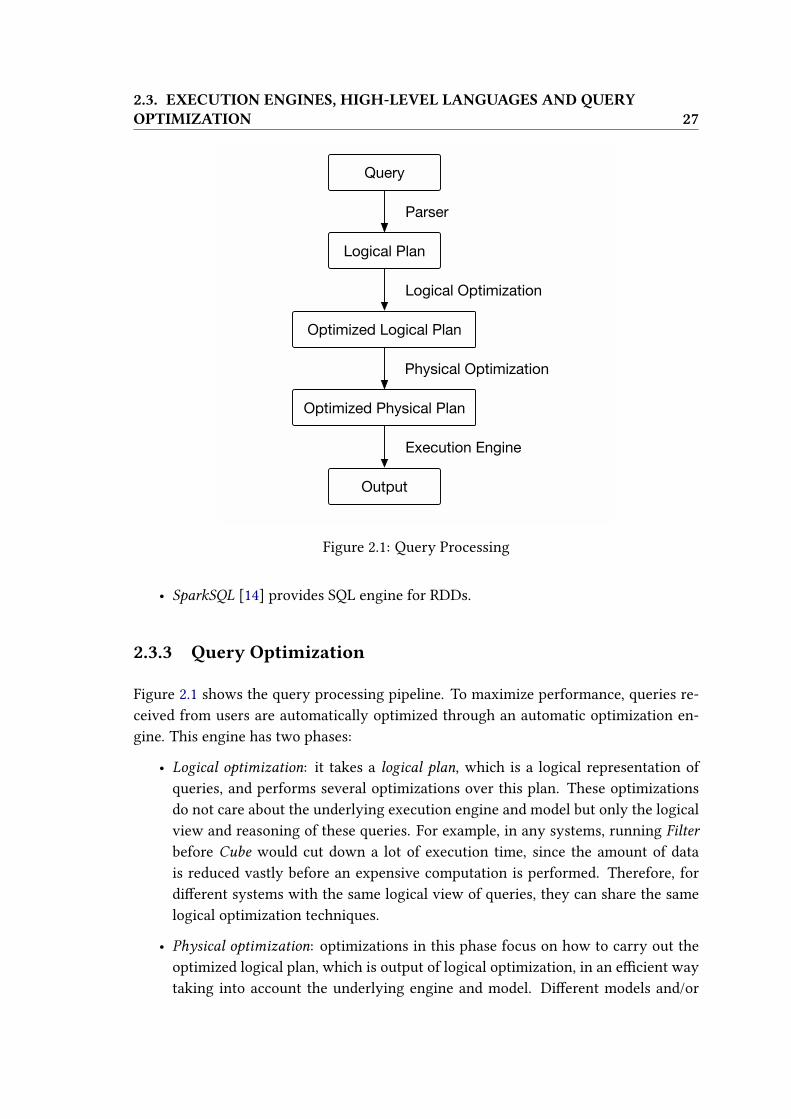
Figure 2.1: Query Processing
• SparkSQL [14] provides SQL engine for RDDs.
2.3.3 Query Optimization
Figure 2.1 shows the query processing pipeline. To maximize performance, queries re-
ceived from users are automatically optimized through an automatic optimization en-
gine. This engine has two phases:
• Logical optimization: it takes a logical plan, which is a logical representation of
queries, and performs several optimizations over this plan. These optimizations
do not care about the underlying execution engine and model but only the logical
view and reasoning of these queries. For example, in any systems, running Filterbefore Cube would cut down a lot of execution time, since the amount of data
is reduced vastly before an expensive computation is performed. Therefore, for
di�erent systems with the same logical view of queries, they can share the same
logical optimization techniques.
• Physical optimization: optimizations in this phase focus on how to carry out the
optimized logical plan, which is output of logical optimization, in an e�cient way
taking into account the underlying engine and model. Di�erent models and/or

28 CHAPTER 2. BACKGROUND
execution engines have di�erent physical optimizations. For instance, for Hadoop
MapReduce, the optimization has to decide how to form a 〈key, value〉 pair, which
is a non-exist thing in traditional databases. The output of this phase is an opti-
mized physical plan, and is ready for execution engine to pick up and carry out to
obtain the �nal results.
2.4 Summary
In this Chapter, we present the basic background of data aggregation and query opti-
mization and give principal reasons behind their enormous importance. We also shed
light on the current most popular large-scale data processing tools, including the pro-
gramming model as well as the execution engines. We remark that, to acknowledge
users’ requirements for optimizing large-scale data aggregation, this dissertation is ca-
pable of providing them:
1. Logical optimization for data aggregation (Chapter 3).
2. Physical optimization for data aggregation (Chapter 4).
3. A automatic query optimization engine that accepts high-level language queries
(Chapter 5).

Chapter 3
Logical Optimization for Large-ScaleData Aggregation
In this Chapter, we present our work on the logical optimization for large-scale data
aggregation.
3.1 Introduction
In this Chapter, we tackle the most general problem in optimizing data aggregation: how
to e�ciently compute a set of data aggregation queries. We remind that, in Section 2.1,
this problem is also equivalent to the problem of how to e�ciently compute a set of
multiple Group By queries. This problem is known to be NP-complete ( [26, 31]), and
all state of the art algorithms ( [24, 26, 31, 32]) use heuristic approaches to approximate
the optimal solution. However, none of prior works scales well with large number of
attributes, and/or large number of queries. Therefore, in this Chapter, we present a novel
algorithm that:
• Scales well with both large numbers of attributes and numbers of Group By
queries. In our experiment, the latency introduced by our query optimization al-
gorithm is several orders of magnitude smaller than that of prior works. As the
optimization latency is an overhead that we should minimize, our approach is truly
desirable.
• Empirically performs better than state of the art algorithms: in many cases our
algorithm �nds a better execution plan, in many other cases it �nds a comparable
execution plan, and in only a few cases it slightly trails behind.
In the rest of the Chapter, we formally describe the problem in Section 3.2. We then
discuss the related work and their limitations in Section 3.3 to motivate the need for a
29

30CHAPTER 3. LOGICAL OPTIMIZATION FOR LARGE-SCALE DATA
AGGREGATION
new algorithm. The details of our solution with a complexity analysis are presented in
Section 3.4 . We continue with our experimental evaluation in Section 3.5. A discussion
about our algorithm and its extension is in Section 3.6. Finally we summarize our work
and present our perspectives in Section 3.7.
3.2 Problem Statement
There are two types of query optimization: single-query optimization and multi-query
optimization. As its name suggest, single-query optimization optimizes a single query
by deciding, for example, which algorithm to run, con�guration to use and optimized
values for parameters. An example is the work in [29]: when users issue a Rollup query
to compute aggregates over day, month and year, the optimization engine automatically
picks the most suitable state of the art algorithms [28] and set the appropriate parameter
to obtain the lowest query response time.
On the other hand, multi-query optimization optimizes the execution of a set of multiple
queries. In large organizations, there are many users who share the same data manage-
ment platform, resulting in a high probability of systems having concurrent queries to
be processed. A cross industry study [71] shows that not all data is equal: in fact, some
input data is “hotter” (i.e. get accessed more frequently) than others. Thus, there are
high chances of users accessing these “hot” �les concurrently. This is also veri�ed by
in industrial benchmarks (TPC-H and TPC-DS) in which their queries frequently access
the same data. The combined outcome is that optimizing multiple queries over the sameinput data can be signi�cantly bene�cial.
The problem we address in this Chapter, the multiple Group By query optimization
(MGB-QO), can come from both scenarios. From the single-query optimization perspec-
tive, any Cube, Rollup or Grouping Sets query is equal to multiple Group Bys. From the
multi-query optimization perspective, the fact that many users issue one Group By over
the same data means multiple Group Bys and it requires optimization. More formally,
we consider an o�ine version of the problem:
• For a time window ω, without loss of generality, we assume the system receives
data aggregation queries over the same input data that contains one of the follow-
ing operators:
– Group By
– Rollup
– Cube
– Grouping Sets
3.2. PROBLEM STATEMENT 31
• These queries correspond to n Group By queries {Q1, Q2, ..., Qn}
In reality, hardly any query arrives at our system at the exact same time. The time win-
dow ω can be interpreted as a period of time in which queries arrive and are treated as
concurrent queries. The value of ω can either be predetermined or dynamically adjusted
to suit the system workload and scheduler, which lead to the online version of this prob-
lem. However, the online problem is not addressed in this dissertation: it remains part
of our future work.
3.2.1 De�nitions
We assume that the input data is a table T with m attributes (columns). Let S =
{s1, s2, ..., sn} be the set of groupings that have to be computed from n queries
{Q1, Q2, ..., Qn}, where si is a subset of attributes of T . Each query Qi is a Group By
query:
Qi: Select si, Count(*) From T Group By si
To simplify the problem, we assume that all queries perform the same aggregate measure
(function) (e.g. Count(*)). Later in Section 3.6.2, we discuss the solution to adapt to
di�erent aggregate measures.
3.2.1.1 Search DAG
Let Att = {a1, ...am} =⋃∞i=1 si be the set of all attributes that appear in n Group By
queries. We construct a directed acyclic search graph G = (V,E) de�ned as follows.
A node in G represents a grouping (or a Group By query). V is the set of all possible
combinations of groupings constructed from Att plus a special node: the root node T .
The root node is essentially the input data itself.
An edge e = (u, v) ∈ E from node u to node v indicates that grouping v can be computed
directly from grouping u. For instance, an edge AB → A means that grouping A can be
computed from grouping AB. There are two costs associated with an edge e between
two nodes: a sort cost csort(e) and a scan cost cscan(e). If groupingAB is sorted in order of
(A,B), computing groupingAwould require no additional sort, but only a scan over the
grouping AB. We denote this cost by cscan(e). However if grouping AB is not sorted,
or sorted in order of (B,A), computing grouping A would require a global sort on the
attribute A, incurring a sort cost csort(e). The costs are of course di�erent in two cases.
We note the only exception: the root node. If input data is not sorted, then all outgoing
edges from the root node have only one sort cost.
We call G a search DAG. Next, we show an example with four queries. In this example,
we have an input table T (A,B,C) and four Group By queries:

32CHAPTER 3. LOGICAL OPTIMIZATION FOR LARGE-SCALE DATA
AGGREGATION
ABC
ACAB BC
CBA
T
Figure 3.1: An example of a search DAG
Q1: Select A, Count(*) From T Group By(A)Q2: Select B, Count(*) From T Group By(B)Q3: Select C, Count(*) From T Group By(C)Q4: Select A,B,Count(*) From T Group By(A,B)
From the above de�nitions, we have:
• S = {A,B,C,AB}.
• Att = {A,B,C}.
• V = {T, ∗, A,B,C,AB,AC,BC,ABC}.
It is easy to see that S ⊆ V . We call S the terminal (or mandatory) nodes: all of these
nodes have to be computed and materialized as these are outputs of our Group By queries
{Q1, Q2, Q3, Q4}. Other nodes in V \ S are additional nodes which may be computed if
it helps to speed up the execution of computingS. In this example, even though grouping
ABC is not required, computing it allows S = {A,B,C,AB} to be directly computed
from ABC rather than the input table T . If the size of ABC is much smaller than T ,
the execution time of S is indeed reduced. Because V contains all possible combinations
of groupings constructed from Att, we are sure that all possible groupings that help
reduce the total execution cost are inspected. We also prune the space of V to exclude
nodes that have no outgoing edges to at least one of the terminal nodes, i.e. these nodes

3.2. PROBLEM STATEMENT 33
certainly cannot be used to compute S. The �nal search DAG for the above example is
shown in Figure 3.1.
Intuitively if a grouping is used to compute two or more groupings, we want to store it
in memory or disk to serve later rather than recompute it.
3.2.1.2 Problem Statement
In data management systems, the problem of multiple Group By query optimization is
processed through both logical and physical optimization. In logical optimization, we set
to �nd an optimal solution tree G′ = (V ′, E ′). The solution tree G′ is a directed subtree
from G, rooted at T , that covers all terminal nodes si ∈ S. It can be seen as a logical
plan for computing multiple Group By queries e�ciently. This is the main objective of
this Chapter.
The physical optimization, as its name suggests, takes care of all physical details to exe-
cute the multiple Group By queries and return actual aggregates. Understandably, di�er-
ent data management systems have di�erent architectures to organize their data layout,
disk access, indexes, etc. Thus, naturally each system may have is own technique to im-
plement the physical multiple Group By operator. For reference purpose, some example
techniques are PipeSort, PipeHash [26], Partition-Cube, Memory-Cube [74] or newer
technique for multiprocessors in [20] for databases, or In-Reducer Grouping [28, 80]
for MapReduce and its extensions. We note that the physical optimization is not this
Chapter’s target: our solution is not a�ected by any particular physical technique. Also,
regardless of the physical techniques, the grouping order is guided by the solution tree
G′ obtained from our logical optimization.
More formally, in the optimized solution tree G′ we have:
1. S ⊆ V ′ ⊆ V .
2. E ′ ⊂ E and for any edge e(u, v) ∈ E ′, there is only one type of cost associated to
edge e:
c(e) =
{csort(e)
cscan(e)
3. From any node u ∈ V ′, there is at most one outgoing scan edge.
An optimal solution tree is the solution tree with the minimal total execution cost
C(E ′) =∑
e∈E′ c(e). Figure 3.2 shows an optimal solution tree for the above exam-
ple. The dotted lines represent sort edges, and the solid lines show the scan edges. The
bold nodes are the required grouping (i.e. terminal nodes). The italic node (ABC) is

34CHAPTER 3. LOGICAL OPTIMIZATION FOR LARGE-SCALE DATA
AGGREGATION
ABC
AB
CA B
T
Figure 3.2: An example of a solution tree
the additional node whose computation helps to reduce the total execution cost of G′.
Additional groupings BC and AC are not computed as doing so does not bring down
the cost of G′.
Finding the optimal solution tree for multiple Group By queries is an NP-complete prob-
lem [31, 51]. State of the art algorithms use heuristic approaches to approximate the
solution. In the next Section, we discuss in more detail why none of those algorithms
scale well with large number of attributes, and/or large number of Group By queries.
This motivates us to �nd a more scalable approach.
3.2.2 Cost model
Our primary goal is to �nd the solution tree G′ with a small total execution cost. The
total execution cost is the sum of the cost from all edges inG′. Therefore, we need a cost
model that assigns the scan and sort costs to all edges in our search graph. However,
our work does not depend on a speci�c cost model as its main purpose is to quantify the
execution time of computing a node (a Group By) from another node. Any appropriate
cost model for various systems like parallel databases, MapReduce systems, etc. can be
plugged into our algorithm.

3.3. RELATEDWORK 35
3.3 Related Work
Optimizing data aggregation in traditional databases has been one of the main tasks
in database research. The multiple Group By query problem are studied through the
lenses of the most general operator in data aggregation: Grouping Sets. The Grouping
Sets is syntactically an easy way to specify di�erent Group By queries at the same time,
therefore all of Group By, Rollup, Cube queries can be translated directly into a Grouping
Sets query.
To optimize Grouping Sets queries, the common approach is to de�ne a directed acyclic
graph (DAG) of nodes, where each node represents a single Group By appearing in the
Grouping Sets query [24, 26, 31, 32, 51]. An edge from node u to node v indicates that
grouping v can be computed from grouping u. For example: groupBC can be computed
from BCD.
There are two major di�erences among various works to compute Grouping Sets. The
�rst di�erence is the cost model: how to quantify a cost (expressed as a weight of an edge)
to compute a group v from a group u. PipeSort [51] sets the weight of an edge (u, v) to
be proportional to the cost of re-sorting u to the most convenient order to compute
v. For example, to compute BC , the main cost would be to resort ABC to BCA to
compute (B,C). This is a sort cost. However, if grouping ABC is already in the sorting
order of (B,C,A), the cost to compute BC would be mainly scan (hence scan cost). In
contrast, [24] and [31] simplify the cost model by having only one weight for each edge
(u, v), regardless of how physically v is computed: the weight of an edge (u, v) is equal
to the cardinality of group u.
The other di�erence is, given a DAG of Group By nodes and weighted edges with appro-
priate costs, how to construct an optimal execution plan that covers all required Group
Bys with the minimum total cost. This problem is proven to be NP-complete ( [31, 51]),
thus approximations through heuristic approaches are studied.
The work in [24] gives a simple greedy approach to address the problem. It considers
Group By nodes in descending order of cardinality. Each Group By is connected to one
of its super nodes. Super nodes of v is any node u such that (u, v) exists. If there are
super nodes that can compute this Group By without incurring a sorting cost, it chooses
the one with the least cost. This Group By becomes a scan child of its parent node. If
all super nodes already have a scan child, it chooses the super nodes with the least sort
cost. This approach is called Smallest Parent. It is simple and fast, however it does not
consider any additional node that can help reducing the total cost. In the rest of this
section, we consider algorithms that include also additional nodes.
In [26], the authors transform the problem into a Minimal Steiner Tree (MST) on directed
graph problem. Because the cost of an edge depends on the sorting order of the parent

36CHAPTER 3. LOGICAL OPTIMIZATION FOR LARGE-SCALE DATA
AGGREGATION
node, a Group By node is transformed into multiple nodes: each corresponds to a sort-
ing order that can be generated (using permutation) from the original Group By node.
Then the approach in [26] adds cost to all pairs of nodes, and uses some established
approximation of MST to retrieve the optimized solution. The main drawback of this
approach is that, the transformed DAG contains a huge number of added nodes and
edges (because of permutation), and even a good approximation of MST problem cannot
produce solutions in feasible time, as any good MST approximation is at least O(|V |2)where |V | is the number of nodes. For example, to compute Cube with 8 attributes, the
transformed DAG consists of 109, 601 nodes and 718, 178, 136 edges, w.r.t. 256 nodes
and 6, 561 edges of the original DAG.
In another work [32], the authors present a greedy approach on the search DAG of
Grouping Sets. Given a partial solution tree T (which initially includes only the root
node), the idea is to consider all other nodes to �nd one that can be added to T with the
most bene�t. When the node x is added to T , it is �rst assumed to be computed from
the input data set, and this incurs a sort cost. Then the algorithm in [32] tries to mini-
mize this cost, by �nding the best parent node from which x can be computed. Once x’s
parent is chosen, this approach �nds all the nodes that are bene�cial if computed from
x rather than its current parent. This bene�t is then subtracted by the cost of adding
x to yield the total bene�t of adding x to T (which the bene�t value can be positive
or negative). This process is repeated until it cannot �nd any node that brings positive
bene�t to add to T. The complexity of this approach isO(|V ||T |2) where |V | = 2m, m is
the number of attributes and |T | is the size of the solution tree, which is typically larger
than the number of terminal nodes (|T | ≥ n). Note that while |V | is much smaller than
the number of nodes in [26] because of no added permutation, it is still problematic if m
is large.
While the approach in [32] is more practical than the approach in [26], it cannot scale
well with a search DAG of a much larger number m of attributes, in which the full
space of additional nodes and edges can not be e�ciently enumerated. To address this
problem, [31] proposes a bottom-up approach. It �rst constructs a naïve plan in which
all mandatory nodes are computed from the input data set. Then from all children nodes
of the input data set, it considers all pairs of nodes (x, y) that can be merged. For each
pair, it computes the cost of a new plan obtained by merging this pair of nodes. After
that, it pick the pair, say (v1, v2), that has the lowest cost and replace the original plan
with this new plan. In this new plan, the node v1 ∪ v2 is included to the solution tree.
In other words, an additional node is only considered and added if and only if it is the
parent of at least two di�erent nodes. This eliminates the task of scanning all nodes in
the search DAG, making this algorithm a major improvement over previously described
algorithms. At some point in time, if all the possible pairs result in a worse cost then
the current plan, the algorithm stops. This algorithm callsO(n3) times the procedure of

3.4. THE TOP-DOWN SPLITTING ALGORITHM 37
merging two nodes where n is the number of terminal nodes. The merging procedure
has the complexity of O(n). Overall, the complexity of this algorithm is O(n4).
The advantage of the algorithm described in [31] is that, it scales irrespectively to the
space of |V | but only to n, the number of Group By queries. If n is small, it scales better
than [26,32]. However, for dense multiple Group By queries, i.e. large n and smallm (e.g.computing Cube of 10 attributes results in n = 1024), this algorithm scale worse than
[26,32]. This motivates us for a more scalable and e�cient algorithm to approximate the
solution tree.
3.4 The Top-Down Splitting Algorithm
In this Section, we propose a heuristic algorithm called Top-Down Splitting to �nd a
solution tree in the multiple Group By query optimization discussed in Section 3.2. Our
algorithm scales well with both large numbers of attributes and large number of Group
By queries. Compared to state of the art algorithms, our algorithm runs remarkably
faster without sacri�cing the e�ectiveness. In Section 3.4.1, we present our algorithm
in detail with its complexity evaluation in Section 3.4.2. Finally, we discuss the choice
of appropriate values for an algorithm-wise parameter, as it a�ects directly the running
time of our algorithm.
3.4.1 Top-Down Splitting algorithm
Our algorithm consists of two steps. The �rst step is to build a preliminary solution tree
that consists of only terminal nodes and the root node. Taking this preliminary solution
tree as its input, the second step aims to repeatedly optimize the solution tree by adding
new nodes to reduce the total execution cost. While the second step sounds similar
to [32], we do not consider the whole space of additional nodes. Instead, we consider
only additional nodes that can evenly split a node’s children into k subsets. Here k is an
algorithm-wise parameter set by users. By trying to split a node’s children into k subsets,
we apply a structure to our solution tree: we transform the preliminary tree into a k-way
tree (i.e. at most k fan-out). Observing the solution trees obtained from state of the art
algorithms, we see that most of the times they have a relatively low fan-out k.
3.4.1.1 Constructing the preliminary solution tree
This step returns a solution tree including only terminal nodes (and of course, the root
node). Later, we further optimize this solution tree. The details of this step are shown in
Algorithm 1.
38CHAPTER 3. LOGICAL OPTIMIZATION FOR LARGE-SCALE DATA
AGGREGATION
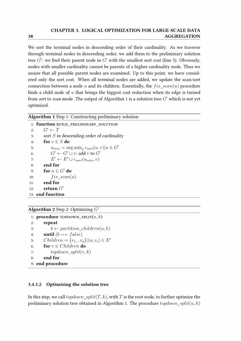
We sort the terminal nodes in descending order of their cardinality. As we traverse
through terminal nodes in descending order, we add them to the preliminary solution
tree G′: we �nd their parent node in G′ with the smallest sort cost (line 5). Obviously,
nodes with smaller cardinality cannot be parents of a higher cardinality node. Thus we
assure that all possible parent nodes are examined. Up to this point, we have consid-
ered only the sort cost. When all terminal nodes are added, we update the scan/sort
connection between a node u and its children. Essentially, the fix_scan(u) procedure
�nds a child node of u that brings the biggest cost reduction when its edge is turned
from sort to scan mode. The output of Algorithm 1 is a solution tree G′ which is not yet
optimized.
Algorithm 1 Step 1: Constructing preliminary solution
1: function build_preliminary_solution
2: G′ ← T3: sort S in descending order of cardinality
4: for v ∈ S do5: umin = argminu csort(u, v)|u ∈ G′6: G′ ← G′ ∪ v: add v to G′
7: E ′ ← E ′ ∪ esort(umin, v)8: end for9: for u ∈ G′ do
10: fix_scan(u)11: end for12: return G′
13: end function
Algorithm 2 Step 2: Optimizing G′
1: procedure topdown_split(u, k)
2: repeat3: b← partition_children(u, k)4: until (b == false)5: Children = {v1...vq}|(u, vi) ∈ E ′6: for v ∈ Children do7: topdown_split(v, k)8: end for9: end procedure
3.4.1.2 Optimizing the solution tree
In this step, we call topdown_split(T, k), with T is the root node, to further optimize the
preliminary solution tree obtained in Algorithm 1. The procedure topdown_split(u, k)

3.4. THE TOP-DOWN SPLITTING ALGORITHM 39
(Algorithm 2) repeatedly calls partition_children(u, k) (Algorithm 3) that splits the
children of node u into at most k subsets. The function partition_children(u, k) re-
turns true if it can �nd a way to optimize u, i.e. split children of node u into smaller
subsets and reduce the total cost. Otherwise, it returns false to indicate that children of
node u cannot be further optimized. We then recursively apply this splitting procedure
to each child node of u. Since the �ow of our algorithm is to start partitioning from the
root down to the leaf nodes, we call it the Top-Down Splitting algorithm.
Algorithm 3 Find the best strategy to partition children of a node u to at most k subsets
1: function partition_children(u, k)
2: CN = {v1...vq}|(u, vi) ∈ E ′3: if q ≤ 1 then . q: number of child nodes
4: return false
5: end if6: Cmin = cost(G′)7: SS ← ∅8: if k > q then9: k = q . constraint: k ≤ q
10: end if11: for k′ = 1→ k do12: A = divide_subsets(u, k′)13: compute the new cost C ′
14: if C ′ < Cmin then15: Cmin ← C ′ . remember the lowest cost
16: SS ← A . remember new addition nodes
17: end if18: end for19: if SS 6= ∅ then20: Update G′ according to SS21: return true
22: else23: return false
24: end if25: end function
The function partition_children(u, k) (Algorithm 3) tries to split the children of u into
at most k subsets. Each of these k subsets is represented by an additional node that is
the union of all nodes in that subset. The intuition is that, instead of computing children
nodes directly from u, we try to compute them from one of these k additional nodes and
check if this reduces the total execution cost. Observing the solution tree obtained from
state of the art algorithms, we see that in many situation, the optimal splitting strategy
may not be exactly k, but a value k′ (1 ≤ k′ ≤ k). By trying every possible split k′ from
1 to k, we compute the new total execution cost with new additional nodes, and retain
the best partition scheme, i.e. the one with the lowest total cost. Then, we update the

40CHAPTER 3. LOGICAL OPTIMIZATION FOR LARGE-SCALE DATA
AGGREGATION
solution graph accordingly: removing edges from u to children, adding new nodes and
edges from u to new nodes, and from new nodes to children of u.
Algorithm 4 Dividing children into k′ subsets
1: function divide_subsets(u, k′)2: CN = {v1...vq}|(u, vi) ∈ E ′3: sort CN by the descending order of cardinality
4: Cmin = cost(G′)5: for i = 1→ k′ do6: SSi ← ∅ . initialize subsets ith
7: end for8: for v ∈ CN do9: imin = argmini attach(v, SSi)|i ∈ 1, ...k′
10: SSimin ← SSimin ∪ v11: end for12: return SS = {SSi}∀1 ≤ i ≤ k′
13: end function
The divide_subsets(u, k′) (Algorithm 4) is called to divide all children of u into k′ sub-
sets and return k′ new additional nodes. At �rst, we sort the children nodes (CN ) in
descending order of their cardinality. As we traverse through these children nodes, we
add each child node into a subset that yields the smallest cost. The cost of adding a child
node v into a subset SSi is:
attach(v, SSi) =[csort(u, SSi ∪ v)
+ csort(SSi ∪ v, v)− csort(u, v)]
Here SSi denotes the additional node representing the ith subset (i ≤ k′). If a node v is
attached to a subset SSi, the new additional node is updated: SSi ← SSi ∪ v.
Now that we have described our two steps, our algorithm is described in Algo-
rithm 5.
Algorithm 5 Top-Down Splitting algorithm
1: G′ = build_preliminary_solution()2: topdown_split(G′.getRoot(), k)
3.4.2 Complexity of our algorithm
In this Section, we evaluate the complexity of our algorithm in the best case and the worst
case scenarios. The average case complexity depends on uncontrolled factors such as:

3.4. THE TOP-DOWN SPLITTING ALGORITHM 41
input data distribution, relationship among multiple Group Bys, speci�c cost models,
etc. We cannot compute the average complexity without making assumptions on such
factors. Therefore this remains part of our future work. Empirically, we observe that in
our experiments the average case leans towards the best case with just a few exceptions
that are closer to the worst case.
3.4.2.1 The worst case scenario
As the �rst step and the second step of our algorithm are consecutive, the overall com-
plexity is the maximum complexity of two steps. It is easy to see that the complexity of
Algorithm 1 is O(n2) where n = |S| is the number of Group By queries.
For the second step, we �rst analyze the complexity of Algorithm 3: it calls O(k)times the divide_subsets function and it computes O(k) times the cost of the modi-
�ed solution tree. The complexity of the divide_subsets function (i.e. Algorithm 4) is
O(max(k2, kq)). As we cannot divide q children nodes into more than q subsets, k ≤ q.
Therefore the complexity of Algorithm 4 is O(kq). It is not di�cult to see that q is
bounded by n, i.e. q ≤ n. The case of q = n happens when all mandatory nodes connect
to the root node. Therefore the worst case complexity of Algorithm 4 is O(kn)
Since Algorithm 3 limits itself in only modifying node u and its children, we can compute
the new cost by accounting only altered nodes and edges. There are at most k new
additional nodes, and there are q children nodes of node u, so computing each time a
new cost of the solution tree is in O(k + q) time. As k ≤ q ≤ n, the complexity of
computing a new cost is O(n), which is smaller than O(kn) of Algorithm 4. As such,
the worst case complexity of Algorithm 3 is O(k2n)
The complexity of Algorithm 2 depends on how many times partition_children is
called. Let |V ′| be the number of nodes in the �nal solution tree. Clearly topdown_split
is called at most |V ′| times, and each time it calls partition_children at least once. In
order for topdown_split to terminate, partition_children has to return false, and it
does so in O(|V ′|) time.
Now, for each time topdown_split is called, partition_children is called more than once
if and only if it returns true, which means at least an additional node is added to V ′.
When an additional node is added, it puts together a new subset, which consists of atleast 2 children nodes or more. In other words, if an additional node is formed, in the
worst case it applies a binary structure to the solution tree that has maximum n leaves
nodes. A property of binary trees states that |V ′| ≤ 2n − 1, which means there are no
more than n−1 additional nodes in the �nal solution tree. As a consequence, in the worst
case, partition_children returns true in essentially O(n) time. Since |V ′| ≤ 2n− 1, it
also returns false in O(|V ′|) ≡ O(n) time.

42CHAPTER 3. LOGICAL OPTIMIZATION FOR LARGE-SCALE DATA
AGGREGATION
T
A
B
C D
BCD
ABCD
CD
Figure 3.3: An example of worst case scenario with k = 2
The worst-case complexity of Algorithm 2 (i.e. our second step) isO(k2n2). AsO(k2n2)
is higher than O(n2) of the �rst step, the worst case complexity of our algorithm is
O(k2n2). Figure 3.3 shows an example of the optimized solution tree obtained in the
worst case scenario.
3.4.2.2 The best case scenario
In the best case scenario, we obtain a balanced k-way solution tree. Figure 3.4 shows
an example of such a balanced solution tree. In this scenario, Algorithm 2 calls
partition_children to return true in O(logkn) times instead of O(n) times like the
worst case scenario. Therefore, the best case complexity is O(k2nlogkn).

3.4. THE TOP-DOWN SPLITTING ALGORITHM 43
T
A B C D
AB CD
ABCD
Figure 3.4: An example of best case scenario with k = 2
3.4.3 Choosing appropriate values of k
Our algorithm depends on an algorithm-wise parameter: k representing the fan-out of
the solution tree. We observe that for solution trees obtained from state of the arts
algorithm, the value of k is rather small. For example, let us consider a primary study
case that motivates the work in [31]: a Grouping Sets query to compute all single-column
Group By in a table withm attributes (i.e. the number of Group By is equal tom). In this
example, small values of k such as 2 ≤ k ≤ 4 are su�cient to �nd an optimized solution
tree. In our experiments in Section 3.5, high values of k do not result in a lower cost
solution tree. We note that our observation is in line to what observed in [31].
For any node u, let qu be the number of its children. Clearly we cannot force to split u’s
children into more than qu subsets, i.e. k ≤ qu. We denote k_maxu = qu. Thus, any
value of k higher than qu is wasteful, and our algorithm does not consider such values
(line 9 in Algorithm 3).
On the other hand, for some node u, we cannot split its children into less than a certain
number of subsets. Let us consider an example in which we want to partition 5 children
nodes of u = ABCDE: ABCD,ABCE,ABDE,ACDE and BCDE. Clearly split-
ting these children nodes into any number of subsets smaller than 5 is not possible, as
merging any pairs of nodes results in the parent node u itself. In this example, 5 is the
minimum number of subsets for node u. Values of k smaller than 5 result in no possible

44CHAPTER 3. LOGICAL OPTIMIZATION FOR LARGE-SCALE DATA
AGGREGATION
splits. We call this the lower bound of k. To �nd an exact lower bound of k in a speci�c
node u is not a trivial task. For instance, let us replace 5 children nodes of u = ABCDE
with: A,B,C,D,E. In this situation, the lower bound of k for node u is 2. We denote
k_minu = 2
As k is an algorithm wise parameter, we have the following: k_minu ≤ k, ∀u ∈ T .
Obviously, we can set k = max(k_minu). However, doing this is not always bene�cial.
Let us continue with our example, as Figure 3.3 and Figure 3.4 suggests, for nodeABCD
and its children (A,B,C,D), k = 2 is su�cient to obtain an optimized solution tree; in
other words, for this node, k = 5 is wasteful.
Algorithm 6 Adaptively dividing children
1: function divide_subsets(u, k′)2: CN = {v1...vq}|(u, vi) ∈ E ′3: sort CN by the descending order of cardinality
4: Cmin = cost(G′)5: p = k′ . p: the current number of subsets
6: for i = 1→ p do7: SSi ← ∅ . initialize subsets ith
8: end for9: for v ∈ CN do
10: imin = argmini attach(v, SSi)|(SSi ∪ v) 6= u11: if imin 6= null then12: SSimin ← SSimin ∪ v13: else14: p← p+ 1 . increase number of subsets
15: SSp ← v . add v to the new subset
16: end if17: end for18: return SS19: end function
In the general case, if we partition children nodes of u into a predetermined number of
subsets k, i) for some node u it could be impossible to partition in such a way; ii) for
some node u′ it may be wasteful. Again, our observation is that most nodes have a very
low fan-outs. Nodes with high upper bound of k are relatively scarce. So our strategy
is to attempt partitioning children nodes of u into small numbers of subsets (i.e., k is
small). Whenever such a split is unachievable, we dynamically increase our number of
subsets until the partition is possible. We modify Algorithm 4 to re�ect the new strategy
(Algorithm 6). The gist of this algorithm is that, we can attach a child node v of u to a
subset SSi if and only if (SSi∪ v) 6= u. When there is no such SSi, we add a new subset
(i.e. at this node, we increase the number of subsets by 1).

3.5. EXPERIMENTS AND EVALUATION 45
3.5 Experiments and Evaluation
An optimization algorithm for the multiple Group By query problem can be evaluated
from three di�erent aspects:
• Optimization latency: the time (in second) that an algorithm takes to return the
optimized solution tree. It is also the optimizing overhead. The lower the opti-
mization latency, the better. This is an important metric to assess the scalability
of an algorithm.
• Solution cost: given a cost model and a solution tree, it is the total of scan and sort
cost associated to edges of the tree. A lower cost means a better tree. This metric
assesses the e�ectiveness of an algorithm.
• Runtime of the solution tree: the execution time (in second) to compute n Group
By queries using the optimized execution plan.
In this Section, we empirically evaluate the performance of our algorithm compared
to other state of the art algorithms. The experimental results of this Section can be
summarized as follows:
• The optimization latency of our algorithm is up to several orders of magnitude
smaller than other algorithms when scaling to both large number of attributes
and large number of Group By queries. In our experiments, the empirical results
suggest that, on average, our algorithm leans towards the best case scenario more
than to the worst case scenario (analyzed in Section 3.4.2).
• We do not sacri�ce the e�ectiveness of �nding an optimized solution cost for low
latency. In fact, compared to other algorithms, in many cases our algorithm �nds
better solutions, in many other cases it �nds comparable ones, and in only a few
cases it slightly trails behind.
• Using PipeSort as the physical implementation to compute multiple Group By
queries, we show that our algorithm can reduce the execution runtime signi�-
cantly (up to 34%) compared to the naïve solution tree, in which all Group Bys are
computed from the input data.
3.5.1 Experiment Setup
The experiments are run on a machine with 8GB RAM. To evaluate the latency and the
solution cost of various algorithms, we synthetically generate query templates. Each
query template consists of i) a list of Group By queries; ii) cardinalities of nodes. The
cardinalities of nodes can be obtained from available datasets using the techniques de-
scribed in [25, 42], or can be randomly generated (with an uniform distribution, or a

46CHAPTER 3. LOGICAL OPTIMIZATION FOR LARGE-SCALE DATA
AGGREGATION
power law distribution to represent skewed data). In some situations (e.g. large number
of attributes), we cannot e�ectively generate all node cardinalities. In this situation, we
take the product of cardinality of each attribute in a node to be the cardinality of that
node.
To evaluate the improvement that an optimized solution tree brings compared to a naïve
one, we issue a query that contains all two-attribute Group Bys from the lineitem table
of TPC-H [23]. This table contains 10 million records with 16 attributes. For each algo-
rithm, we report its optimization latency as well as the query runtime obtained when
we execute the PipeSort operator guided by its solution tree.
The state of the art algorithms that we compare are the ones presented in [32] and in [31].
We omit the algorithm presented in [26] because it is shown to be inferior to the algo-
rithm in [32]. For convenience, we name our algorithm Top-Down Splitting or TDS, the
one in [31] Bottom-Up Merge (BUM), and �nally the one in [32] Lattice Partial Cube or
LPC. For the case of our algorithm, as k can have multiple values, we evaluate both cases:
small value k = 3 and large value k = n.
3.5.2 Cost model in our experiments
As discussed in Section 3.2.2, we need a cost model to assign scan and sort cost to edges
of the search graph. In our experiments, we use a simple cost model as a representative
in evaluating all di�erent algorithms to �nd G′. Again, we stress that any appropriate
cost model can be used. We de�ne the two costs of an edge as follows:
• Scan cost: cscan(u→ v) = |u| where |u| is the size (cardinality) of node u
• Sort cost: csort(u→ v) = |u| ∗ log2|u|
We assume that the cardinality of any node u is readily available: estimating |u| is not
the focus of our work, and we rely on works of cardinality estimation such as [25, 42].
Clearly, a bad cardinality estimation worsen the quality of a solution tree, but all algo-
rithms su�er from the same issue.
3.5.3 Scaling with the number of attributes
In this experiment, we generate the query templates as follows: i) each query template
consists of all single-column (or single-attribute) Group By be generated from a table
T ; ii) the number of attributes, m, in table T is from 5 to 49; iii) for each number of
attributes, we randomly generate 100 di�erent sets of grouping cardinalities, in which
50 sets have uniform distribution, and 50 sets have power law distribution with α = 2.5.

3.5. EXPERIMENTS AND EVALUATION 47
Number of attributes5 10 15 20 25 30 35 40 45 50
Optim
ization L
ate
ncy (
second)
0
2
4
6
8
10
12
14
16
18
BUMLPCTDS k=3TDS k=n
Figure 3.5: Single-attribute Group By - Optimization latency.
Number of attributes
5 10 15 20 25 30 35 40 45 50
Norm
alized S
olu
tion
Cost
0.75
0.8
0.85
0.9
0.95
1
1.05
BUM
LPC
TDS k=3
TDS k=n
Figure 3.6: Single-attribute Group By - Normalized solution cost.
For each number of attributes and algorithm, we compute the average of the solution cost
of the optimized solution tree; as well as the average of its optimization latency.
The results for optimization latency are plotted in Figure 3.5. The latency of the Lattice
Partial Cube algorithm exponentially increases with the number of attributes. This is
in line with its complexity of O(2m|T |2) where m is the number of attributes. For the
sake of readability, we omit the latency of LPC for large number of attributes. In this

48CHAPTER 3. LOGICAL OPTIMIZATION FOR LARGE-SCALE DATA
AGGREGATION
experiment, with its complexity of O(n4) the Bottom-Up Merge latency scales better
than LPC. Nevertheless, as the line of BUM starts to take o� at the end, we expect that
for large n (e.g. n ≥ 100), BUM has a rather high optimization latency. Our algorithm
achieves the best scalability: it takes less than 0.01 second to optimize n = 49 queries
for both cases of k: k = 3 and k = n. Understandably, the latency of TDS with k = n
is higher than TDS with k = 3. However, as both cases have very small latencies, this is
indistinguishable in Figure 3.5.
We note that the solution cost depends on the cost model, and our cost model (see Sec-
tion 3.5.2) depends on grouping cardinalities, which are di�erent in every query template
we generate. Thus, we normalize every cost to a fraction of the solution cost obtained
by a baseline algorithm (here we choose BUM) so that it is easier to compare the solu-
tion costs obtained by di�erent algorithms. The normalized solution costs are shown in
Figure 3.6. Due to the large amount of time for LPC to complete with large number of
attributes m, we skip running LPC for m ≥ 20. For most number of attributes, on aver-
age, our algorithm �nds better solution trees than BUM, sometimes its cost is up to 20%
smaller. Only in few query templates, our solution tree’s cost is a little higher (within
1.5%) than BUM. Compared to LPC, TDS produces comparable execution plans. We no-
tice several spikes of TDS and LPC. The reason is because BUM merges 2 Group Bys at a
time and tends to produce uneven subsets, especially when the number of queries is an
odd number. However, for some queries, BUM merging results in even subsets. In this
case, its solution trees are close to TDS and LPC - thus the spikes.
Table 3.1 shows the average of solution costs obtained by each algorithm for every query
template, normalized to fractional costs of BUM. Altogether, our algorithm is a little bet-
ter than LPC. Also as expected, the execution cost acquired by TDS k = 3 is a little higher
than for k = n, however by not much (less than 0.5%). In summary, our results indicate
that for a comparable, and often lower cost than that of prior works, our approach yields
substantial savings in optimization latency and scalability.
Algorithm BUM LPC TDS k = 3 TDS k = nNormalized Cost 1 0.9419 0.9406 0.9361
Table 3.1: Average solution cost - Single-attribute queries
3.5.4 Scaling with the number of queries
In this experiment, we assess the scalability of various algorithms with respect to the
number of queries. To ful�ll such a goal, we limit the number of attributes to be very
small (3 ≤ m ≤ 9), and generate the query templates for a Cube query, i.e. all possi-
ble combination of Group By queries. The node cardinalities are generated similarly to
Section 3.5.3.

3.5. EXPERIMENTS AND EVALUATION 49
Number of attributes in the CUBE query3 4 5 6 7 8 9
Op
tim
iza
tio
n L
ate
ncy (
se
co
nd
)
10-3
10-2
10-1
100
101
102
103
104
BUMLPCTDS k=3TDS k=n
Figure 3.7: Cube queries - Optimization latency
Number of attributes in the CUBE query3 4 5 6 7 8 9
Norm
aliz
ed S
olu
tion C
ost
0.75
0.8
0.85
0.9
0.95
1
1.05
BUMLPCTDS k=3TDS k=n
Figure 3.8: Cube queries - Normalized solution cost
The optimization latency for this experiment is in Figure 3.7. To emphasize the di�erence
in latency between two cases TDS k = 3 and TDS k = n, we select the log scale for the
y-axis. From Figure 3.7, we see that the latency of TDS k = 3 is slightly lower than TDS
k = n. Nevertheless, in both cases our algorithm still scales remarkably better than other

50CHAPTER 3. LOGICAL OPTIMIZATION FOR LARGE-SCALE DATA
AGGREGATION
algorithms. With m = 9, there are 29 = 512 number of queries: it takes our algorithm
less than 0.1 second to complete. As we mentioned in Section 3.3, in the case of dense
multiple Group By queries, i.e. large n and small m, the BUM algorithm actually scales
worse than the LPC algorithm (of which the complexity in the case of a Cube query of
becomes O(n3)).
Figure 3.8 shows the solution cost of di�erent algorithms in a Cube query. Despite having
the highest latency and thus more time to generate optimized plans, the BUM algorithm
does not produce the best solution tree (i.e. lowest execution cost). The reason is that
BUM starts the optimization process from a naïve solution tree where all nodes are com-
puted directly from the input data. For each step, BUM considers all possible pairs to
merge and it selects the one with the lowest cost. As BUM is a gradient search approach,
for large number of queries, there are too many paths that can lead to local optimum.
In contrast to BUM, LPC and TDS start the optimization process from a viable solution
tree T , which i) has much lower cost compared to the naïve solution tree; ii) has far
less cases (e.g. paths) to consider. In the case of a Cube query, the initial solution tree
T in LPC and TDS is closely similar to the �nal solution tree, with only some minor
modi�cations. This helps both algorithms to achieve much lower latency. Between our
algorithm and LPC, generally the solution tree obtained by LPC is slightly better than
TDS (both cases). However, the di�erences are within 1.5%, which is acceptable if we
want to trade e�ectiveness in �nding solution tree for better scalability. For example,
whenm = 9, our algorithm runs in less than 0.05 second, while LPC runs in 1.5 second.
Between two cases of TDS, we actually �nd very similar solution trees since they both
start from similar preliminary trees.
3.5.5 Scaling with both number of queries and attributes
In this experiment, we compare optimization algorithms by scaling both the aforemen-
tioned factors at the same time: number of attributes and number of queries. To achieve
such a goal, we design the query templates to include all two-attribute Group By queries
from a table T . We set the number of attributesm from 5 to 21, and this makes the num-
ber of queries, which is
(m2
), increase as well. The grouping cardinalities are generated
similarly to Section 3.5.3.
The optimization latency shown in Figure 3.9 exhibits the same traits that we observe in
Sections 3.5.3 and 3.5.4. For low number of attributes, LPC has lower latencies compared
to BUM. However, the space of additional nodes scales exponentially with the number
of queries, so starting from m = 15 (n = 91), optimization latency of BUM gets smaller
than that of LPC. Unsurprisingly, our algorithm has distinctly low overhead. In fact,
the experimental results give us strong con�dence that our algorithm is ready to scale
up to hundreds or even thousands of attributes and queries. An end-to-end evaluation

3.5. EXPERIMENTS AND EVALUATION 51
Number of queries30 60 90 120 150 180 210
Optim
izatio
n L
ate
ncy (
second)
10-4
10-3
10-2
10-1
100
101
102
103
BUMLPCTDS k=3TDS k=n
Figure 3.9: Two-attribute Group By - Optimization latency
Number of Queries
30 60 90 120 150 180 210
Norm
alized S
olu
tion
Cost
0.7
0.75
0.8
0.85
0.9
0.95
1
1.05
BUM
LPC
TDS k=3
TDS k=n
Figure 3.10: Two-attribute Group By - Normalized solution cost
of our optimization techniques handled with the physical implementation of Group By
operators is part of our on-going work, which will ultimately validate the scalability and
e�ciency of our approach.
Figure 3.10 shows the solution cost of di�erent algorithms. Again, we normalize it to a
fraction of the BUM total cost. In some cases, we have spikes where BUM merging results
in even subsets, which is also the goal of TDS. In most cases, TDS actually �nds smaller

52CHAPTER 3. LOGICAL OPTIMIZATION FOR LARGE-SCALE DATA
AGGREGATION
solution costs than that of BUM. Even in minor cases where TDS trails behind BUM,
the di�erence is less than 3%, which is acceptable considering such a low optimization
latency it brings. Table 3.2 presents the total average of execution cost obtained from
each algorithm. An interesting observation here is that, despite having as much as 5
times the latency of TDS k = 3 (see Figure 3.9), the solution tree returned by TDS k = n
actually has less than 1% smaller total cost on average. In general, our solution trees
have lower execution cost than LPC, but not by much. For some cases, both LPC and
our algorithm �nd signi�cantly smaller solution trees than BUM.
Algorithm BUM LPC TDS k = 3 TDS k = nFractional Cost 1 0.9186 0.8760 0.8732
Table 3.2: Average solution cost - Two attribute queries
3.5.6 The impact of cardinality skew
As we mention in Section 3.5.3, the node cardinalities are randomly generated with two
di�erent distributions: uniform and power law with α = 2.5. Overall, the skew intro-
duced by the power law distribution does not a�ect the latency of our algorithm: on
average, queries generated from both distributions have roughly the same runtime1. In
spite of that, the total cost obtained from skewed cardinalities is generally higher than
the solution cost from uniform cardinalities. On average, it is 6.8% higher, with some
particular cases that are up to 18% higher. Our explanation is that, for uniform cardinali-
ties, it is easier to evenly partition children nodes into subsets, while skewed cardinalities
tend to return a very big subset and many small subsets. As a very big subset is used to
compute other nodes, most likely it increases the solution cost by a large margin.
3.5.7 Quality of solution trees
A solution tree is a logical plan to direct the physical operator to execute multiple Group
By operator. A solution tree G′1 is of higher quality than a solution tree G′2 if the run-
time to execute G′1 is smaller than the runtime to execute G′2. In this experiment, we
implement the PipeSort algorithm as the physical operator to execute the solution trees
returned from TDS, LPC and BUM. We also execute a naïve solution tree to prepare a
baseline for comparison.
The dataset we use in this experiment is the lineitem table from the industrial bench-
mark TPC-H [23]. It contains 10 million records with 16 attributes. Our query consists
1Uniform distribution has a slightly higher running time of 1.4%

3.5. EXPERIMENTS AND EVALUATION 53
AlgorithmsBUM LPC TDS Naive
Tim
e (
se
co
nd
)
0
200
400
600
800Optimization Latency
Query Runtime
Figure 3.11: The optimization latency and query runtime.
PPPPPPPPP
Algorithm
BUM LPC TDS Naïve
Optimization Latency (s) 66 87 0.17 0
Query Runtime (s) 632 551 547 826
Total Runtime (s) 698 638 547.17 826
Improvement (%) 15.49 22.76 33.75 0
Table 3.3: The optimization latency and query runtime
of all two-attribute Group Bys from lineitem. For each algorithm, we report, in Fig-
ure 3.11, its optimization latency as well as its query runtime. Detail numbers found
in Table 3.3 indicate that multiple Group By query optimization techniques actually re-
duce the query runtime over a naïve solution. We observe that, in this workload, the
optimization latency of TDS is almost 0% of the total runtime. This is in contrast to that
of BUM (9.45%) and LPC (13.63%). With BUM and LPC, since the optimization latency
contributes a non-negligible part to the total runtime, instead of 23.48% and 33.29%
improvement respectively, they improve only 15.49% and 22.76%. Also, we note that
the solution trees of LPC and our algorithm, TDS, are identical. This lead to the virtually
same query runtime. Nevertheless, overall our algorithm provides greater performance
boost because of its close-to-zero latency.

54CHAPTER 3. LOGICAL OPTIMIZATION FOR LARGE-SCALE DATA
AGGREGATION
3.6 Discussions and Extensions
In this Section, �rst we discuss about the intuition of our algorithm, and attempt to ex-
plain why its solution cost may be better than other algorithms in many cases. Then
we discuss about solutions to extend our algorithm to handle di�erent aggregate func-
tions.
3.6.1 Intuition and Discussion
In the multiple Group By query optimization problem, to design a scalable algorithm, the
�rst building block to consider is how to explore the potential additional groupings (i.e.nodes) to include in a solution. As the space of additional groupings can be very large,
they cannot be e�ectively generated. Therefore, to scale to a large number of queries
and attributes, we cannot explore all possible additional groupings. A more scalable
approach is to consider merging terminal nodes to form new groupings, as the subset
of these additional groupings is much likely considerably smaller than their full space.
Both our algorithm and BUM in [31] use this approach.
The di�erence between TDS and BUM is the process to construct new groupings. At
each step, BUM only considers merging two groupings into a new one. Meanwhile,
TDS evaluates splitting all children nodes of a grouping into at most k subsets, each
with a new grouping. The implication of these steps on the algorithm’s complexity is
already discussed in Section 3.3 and 3.4.2. Here, we intuitively discuss why, in general,
we believe that TDS can produce better solution trees than BUM. The main reason is
because TDS makes a more “global” decision than BUM at each step of their process.
When considering partitioning children nodes, TDS uses available information at the
moment: i) cardinalities of all nodes; ii) associated costs to pair of nodes; iii) multiple
ways to split. In addition, while it is making a decision of putting together a new group-
ing, TDS inspects the connection of this newly formed grouping with respect to all other
groupings available. As a top-down approach, when TDS triggers a splitting decision in
a high-level grouping (e.g. the root node), it dramatically decreases the total execution
cost. Even though the subtree optimization might be far from optimal, early decisions
are more important.
In contrast, the merging process in BUM solely depends on two individual nodes. With
so little information at hand, BUM tends to trigger groupings that decrease the solution
cost by a relatively small margin (because BUM is a bottom-up approach). In addition,
since the initial solution tree is a naïve solution, there are so many pairs of nodes such
that inspecting the potential merging of all pairs leads to a local optimum.

3.6. DISCUSSIONS AND EXTENSIONS 55
3.6.2 Di�erent Aggregate Functions
The multiple Group By optimization problem is based on the premise that a Group By
can be computed from the results of another Group By, instead of the input data. To
assure this property, the aggregate measure (function) must be either distributive, or al-gebraic [64]: fortunately, almost all common aggregate functions are so. Let us consider
an input data T which is split into p chunks Ci. A function F is:
• Distributive if there is a function G such that: F (T ) =
G(F (C1), F (C2), ..., F (Cp)). Usually, for many distributive functions like
Min,Max, Sum, etc., G = F . For G 6= F , an example is Count which is also
distributive with G = sum().
• Algebraic if there are functions G and H such that:
F (T ) = H(G(C1), G(C2), ..., G(Cp)). Examples are
Average,MinN,MaxN, Standard_deviation. In function Average, for
instance, G is to collect the sum of elements and the number of elements, while
H adds up these two components and divides the global sum by the total number
of elements from all the chunks to obtain �nal results.
Thus far, we have assumed that all Group By queries compute the same aggregate func-
tion (Count(∗) in our example). Typically this is the case in single-query optimization
when a user issues a Grouping Sets query. Nonetheless in multi-query optimization,
more often the aggregate functions are di�erent. An easy way to adapt our solution to
di�erent aggregate functions is to separate Group By queries into groups of the same
aggregate function. However, this approach may decrease the opportunity to share pre-
computed Group Bys, and it may end up computing a large portion of Group Bys from
the input data (or from a much larger Group Bys). For instance, let us consider the fol-
lowing queries:
Q1: Select A, Count(*) From T Group By(A)Q2: Select B, Sum(v) From T Group By(B)
Here v is an integer value in table T . Using the aforementioned approach we end up
with both Group Bys A and B computed from the input data T .
Another approach is to apply our optimization to the set of all Group Bys queries. For a
Group By, not only its aggregates are computed, but also are all those of their successors.
To continue our example, our algorithm suggests computing groupingAB from T , then
A and B from AB. When computing AB from T , we evaluate and store both aggre-
gates, Count(∗) and Sum(v). At this moment, Group By Q1 is obtained from grouping
AB with aggregate Count(∗), while we use AB with aggregate Sum(v) to calculate
Group By Q2. The downside of this approach is to incur the cost of storing potentially
numerous intermediate aggregates.

56CHAPTER 3. LOGICAL OPTIMIZATION FOR LARGE-SCALE DATA
AGGREGATION
For systems in which the storage cost is relatively expensive compared to reading/sort-
ing a large amount of data, the �rst approach may be preferred. For other systems, in
which the sorting cost is relatively expensive (e.g. it requires a global shu�e of data
over network), the second approach may be a more viable option. Facilitating users in
making the right choice of approaches is the challenge that we will tackle in our future
work.
3.7 Summary
Data aggregation is a crucial task to understand and interact with data. This is exacer-
bated by the increasingly large amount of data that is collected nowadays. Such data
is often multi-dimensional, characterized by a very large number of attributes. This
calls for the design of new algorithms to optimize the execution of data aggregation
queries.
In this Chapter, we presented our method to address the general problem of optimizing
multiple Group By queries, thus �lling the gap left by current proposals that cannot scale
in the number of concurrent queries or the number of attributes each query can handle.
We have shown, both theoretically and experimentally, that our algorithm incurs in ex-
tremely small latencies, compared to alternative algorithms, when producing optimized
query plans. This means that, in practice, our algorithm can be applied at the scale that
modern data processing tasks require, dealing with data of hundreds of attributes and
executing thousands of queries. In addition, our experimental evaluation illustrated the
e�ectiveness of our algorithm to �nd optimized solution trees. In fact, in many cases,
our algorithm outperformed others in terms of producing optimized solutions, while
being remarkably faster. Finally, we discussed about the intuition behind our algorithm
and the possible approaches to extend it to handle general, heterogeneous queries in
terms of diversity of aggregate functions. A version of this Chapter is published in the
International Conference on Data Engineering 2016 [30].
We conclude this Chapter by noting that our algorithm can be easily integrated to cur-
rent optimization engines of relational databases, to traditional data warehouses or to
modern big-data systems like Apache Hadoop [1], Apache Spark [2]. Instead, using
our algorithm to optimize query execution on recent systems such as Hadoop, Spark
and their respective high-level, declarative interfaces, requires the development of an
appropriate cost model as well as an optimization engine to transform original query
plans into optimized ones. We cover this in Chapter 5. In the next Chapter, Chapter 4,
we continue the �ow of our query optimization and go on to the next phase: physical
optimization.

3.7. SUMMARY 57
Relevant Publications
• D. H. Phan and P. Michiardi, “A novel, low-latency algorithm for multiple group-
by query optimization”, in 32nd IEEE International Conference on Data Engineering,
2016.


Chapter 4
Physical Optimization for DataAggregation
This Chapter presents our contributions in physical optimization for data aggregation:
i) our novel algorithms for data aggregation; ii) our light-weight, cost-based optimization
module.
4.1 Design Space of MapReduce-like Rollup Data Ag-gregates
4.1.1 Introduction
Despite the tremendous amount of work carried out in the database community to come
up with e�cient ways of computing data aggregates, little work has been done to ex-
tend these lines of work to cope with massive scale. Indeed, the main focus of prior
works in this domain has been on single server systems or small clusters executing a
distributed database, implementing e�cient implementations of Grouping Sets, Cube
and Rollup operators, in line with the expectations of low-latency access to data sum-
maries [51,58,61,65,66,74]. Only recently, the community devoted attention to solve the
problem of computing data aggregates at massive scales using large-scale data-intensive
computing engines such as Hadoop [1] and Spark [2] . In support of the growing interest
in computing data aggregates on batch-oriented systems, several high-level languages
built on top of Hadoop MapReduce, such as PIG [8] and HIVE [7], support simple im-
plementations of, for example, the Rollup operator.
The endeavor of this work is to take a systematic approach to study the design space of
the Rollup operator: besides being widely used on its own, Rollup is also a fundamental
59

60 CHAPTER 4. PHYSICAL OPTIMIZATION FOR DATA AGGREGATION
building block used to compute more general data aggregation queries (e.g. Grouping
Sets [30, 52]). We discuss this in more details in Section 4.3. In this Section, we study
the problem of de�ning the design space of algorithms to implement Rollup through
the lenses of a recent model of MapReduce-like systems [49]. The model explains the
trade-o�s that exist between the degree of parallelism that is possible to achieve and the
communication costs that are inherently present when using the MapReduce program-
ming model. In addition, we overcome current limitations of the model we use (which
glosses over important aspects of MapReduce-like computations) by extending our anal-
ysis with an experimental approach. We present instances of algorithmic variants of the
Rollup operator that cover several points in the design space, implement and evaluate
them using a Hadoop cluster.
In summary, our contributions are the following:
• We study the design space that exists to implement Rollup and show that, while it
may appear deceivingly simple, it is not a straightforward embarrassing parallel
problem. We use modeling to obtain bounds on parallelism and communication
costs.
• We design and implement new Rollup algorithms that can match the bounds we
derived, and that swipe the design space we were able to de�ne.
• We pinpoint the essential role of combiners (an optimization allowing pre-
aggregation of data, which is available in real instances of the MapReduce
paradigm, such as Hadoop [1]) for the practical relevance of some algorithm in-
stances, and proceed with an experimental evaluation of several variants of Rollup
implementations, both in terms of their performance (runtime) and their e�cient
use of cluster resources (total amount of work).
• Finally, our Rollup implementations exist in Java MapReduce and have been inte-
grated in our experimental branch of PIG, which are available in a public reposi-
tory.1
The remainder of this Section is organized as follows. Section 4.1.2 provides background
information on the model we use in our work and presents related work. Section 4.1.3 il-
lustrates a formal problem statement and Section 4.1.4 presents several variants of Rollup
algorithms. Section 4.1.5 outlines our experimental results to evaluate the performance
of the algorithms we introduce in this work. The summary of the work in this Section
is presented in Section 4.4.
1h�ps://bitbucket.org/bigfootproject/rollupmr

4.1. DESIGN SPACE OF MAPREDUCE-LIKE ROLLUP DATA AGGREGATES 61
4.1.2 Background and Related Work
We assume the reader to be familiar with the MapReduce [60] paradigm and its open-
source implementation Hadoop [1, 75]. First, we give a brief summary of the model
introduced by Afrati et al. [49], which is the underlying tool we use throughout our
Section. Then, we present related works that focus on the MapReduce implementation
of popular data analytics algorithms.
The MapReduce model. Afrati et al. [49] recently studied the MapReduce program-
ming paradigm through the lenses of an original model that elucidates the trade-o�
between parallelism and communication costs of single-round MapReduce jobs. The
model de�nes the design space of a MapReduce algorithm in terms of replication rateand reducer-key size. The replication rate r is the average number of 〈key, value〉 pairs
created from each input in the map phase, and represents the communication cost of a
job. The reducer-key size q is the upper bound of the size of list of values associated
to a reducer-key. Jobs have higher degrees of parellelism when q is smaller. For some
problems, parallelism comes at the expense of larger communication costs, which may
dominate the overall execution time of a job.
Afrati et al. show how to determine the relation between r and q. This is done by �rst
bounding the amount of input a reducer requires to cover its outputs. Once this relation
is established, a simple yet e�ective “recipe” can be used to relate the size of the input
of a job to the replication rate and to the bounds on output covering introduced above.
As a consequence, given a problem (e.g., �nding the Hamming distance between input
strings), the model can be used to establish bounds on r and q, which in turn de�ne the
design space that instances of algorithms solving the original problem may cover.
Relatedwork. Designing e�cient MapReduce algorithms to implement a wide range of
operations on data has received considerable attention recently. Due to space limitations,
we cannot give justice to all works that addressed the design, analysis and implemen-
tation of graph algorithms, clustering algorithms and many other important problems:
here we shall focus on algorithms to implement SQL-like operators. For example, the
relational JOIN operator is not supported directly in MapReduce. Hence, attempts to
implement e�cient JOIN algorithms in MapReduce have �ourished in the literature:
Blanas et al. [59] studied Repartition Join, Broadcast Join, and Semi-Join. More recent
work tackle more general cases like theta-joins [72] and multi-way-joins [50].
With respect to OLAP data analysis tasks such as Cube and Rollup, e�cient MapReduce
algorithms have only lately received some attention. A �rst approach to study Cube and
Rollup aggregates has been proposed by Nandi et al. [69]; this algorithm, called “naive”
by the authors, is called Vanilla in this work. MR-Cube [69] mainly focuses on algebraic

62 CHAPTER 4. PHYSICAL OPTIMIZATION FOR DATA AGGREGATION
aggregation functions, and deals with data skew; it implements the Cube operator by
breaking the algorithm in three phas-es. A �rst job samples the input data to recognize
possible reducer-unfriendly regions; a second job breaks those regions into sub-regions,
and generates corresponding 〈key, value〉 pairs to all regions, to perform partial data
aggregation. Finally, a last job reconstructs all sub-regions results to form the complete
output. The MR-Cube operator naturally implements Rollup aggregates. However in
the special case of Rollup, the approach has two major drawbacks: it replicates records
in the map phase as in the naive approach and it performs redundant computation in
the reduce phase.
For the sake of completeness, we note that one key idea of our work (in-reducer group-
ing) shares similar traits to what is implemented in the Oracle database [52]. However,
the architectural di�erences with respect to a MapReduce system like Hadoop, and our
quest to explore the design space and trade-o�s of Rollup aggregates make such work
complementary to ours.
4.1.3 Problem Statement
We now de�ne the Rollup operation as a generalization of the SQL Rollup clause, in-
troducing it by way of a running example. We use the same example in Section 4.1.4
to elucidate the details of design choices and, in Section 4.1.5, to benchmark our re-
sults.
Rollup can be thought of as a hierarchical Group By at various granularities, where the
grouping keys at a coarser granularities are a subset of the keys at a �ner granular-
ity. More formally, we de�ne the Rollup operation on an input data set, an aggregationfunction, and a set of n hierarchical granularities:
• We consider a data set akin to a database table, with M columns c1, . . . , cM and L
rows r1, · · · rL such that each row ri corresponds to the (ri1, . . . , riM) tuple.
• Given a set of rows R ⊆ {r1, · · · rL}, an aggregation function f(R) produces our
desired result.
• n granularities d1, . . . , dn determine the groupings that an input data is subject to.
Each di is a subset of
{c1, · · · cM}, and granularities are hierarchical in the sense that di ( di+1 for each
i ∈ [1, n− 1].
The Rollup computation returns the result of applying f after grouping the input by
the set of columns in each granularity. Hence, the output is a new table with tuples
corresponding to grouping over the �nest (dn) up to the coarsest (d1) granularity,

4.1. DESIGN SPACE OF MAPREDUCE-LIKE ROLLUP DATA AGGREGATES 63
denoting irrelevant columns with an ALL value [64].
Example. Consider an Internet Service provider which needs to compute aggregate
tra�c load in its network, per day, month, year and in overall. We assume input data
to be a large table with columns (c1, c2, c3, c4) corresponding to (year, month, day, pay-
load2). A few example records from this dataset are shown in the following:
(2012, 3, 14, 1)(2012, 12, 5, 2)(2012, 12, 30, 3)(2013, 5, 24, 4)
The aggregation function f outputs the sum of values over the c4 (payload) column.
Besides SUM, other typical aggregation functions are MIN, MAX, AVG and COUNT; it is
also possible to consider aggregation functions that evaluate data in multiple columns,
such as for example correlation between values in di�erent columns.
Input granularities are d1 = ∅, d2 = {year}, d3 = {year,month}, and d4 = {year,month, day}. The highest granularity, d1 = ∅, groups on no
columns and is therefore equivalent to a SQL Group By ALL clause that computes the
overall sum of the payload column; such an overall aggregation is always computed in
SQL implementations, but it is not required in our more general formulation. We will
see in the following that “global” aggregation is problematic in MapReduce.
In addition to aggregation on hierarchical time periods as in this case, Rollup aggrega-
tion applies naturally to other cases where data can be organized in tree-shaped tax-
onomies, such as for example country-state-region or unit-department-employee hier-
archies.
If applied on the example, the Rollup operation yields the following result (we use ‘*’ to
denote ALL values):
(2012, 3, 14, 1)(2012, 3, *, 1)(2012, 12, 5, 2)(2012, 12, 30, 3)(2012, 12, *, 5)(2012, *, *, 6)(2013, 5, 24, 4)(2013, 5, *, 4)(2013, *, *, 4)( *, *, *, 10)
2In Kilobytes

64 CHAPTER 4. PHYSICAL OPTIMIZATION FOR DATA AGGREGATION
Rows with ALL values represent the result of aggregation at coarser granularities: for
example, the (2012, *, *, 6) tuple is the output of aggregating all tuples from
year 2012.
Aggregation Functions andCombiners. In MapReduce, it is possible to pre-aggregate
values computed in mappers by de�ning combiners. We will see in the following that
combiners are crucial for the performance of algorithms de�ned in MapReduce. While
many useful aggregation functions are subsceptible to being optimized through combin-
ers, not all of them are. Based on the de�nition by Gray et al. [64], when an aggregation
function is holistic there is no constant bound on the size of a combiner output; repre-
sentative holistic functions are MEDIAN, MODE and RANK.
The algorithms we de�ne are di�erently subsceptible to the presence and e�ectiveness
of combiners. When discussing the merits of each implementation, we also consider the
case where aggregation functions are holistic and hence combiners are of little or no
use.
4.1.4 The design space
We explore the design space of Rollup, with emphasis on the trade-o� between com-
munication cost and parallelism. We �rst apply a model to obtain theoretical bounds
on replication rate and reducer key size; we then consider two algorithms (Vanilla and
In-Reducer Grouping) that are at the end-points of the aforementioned trade-o�, hav-
ing respectively maximal parallelism and minimal communication cost. We follow up
by proposing various algorithms that operate in di�erent, and arguably more desirable,
points of the trade-o� space.
4.1.4.1 Bounds on Replication and Parallelism
Here we adopt the model by Afrati et al. [49] to �nd upper and lower bounds for the
replication rate. Note that the model, unfortunately, does not account for combiners nor
for multi-round MapReduce algorithms.
First, we de�ne the number of all possible inputs and outputs to our problem, and a
function g(q) that allows to evaluate the number of outputs that can be covered with i
input records. To do this, we refer to the de�nitions in Section 4.1.3:
1. Input set: we call Ci the number of di�erent values that each column ci can take.
The total number of inputs is therefore |I| =∏M
i=1Ci.
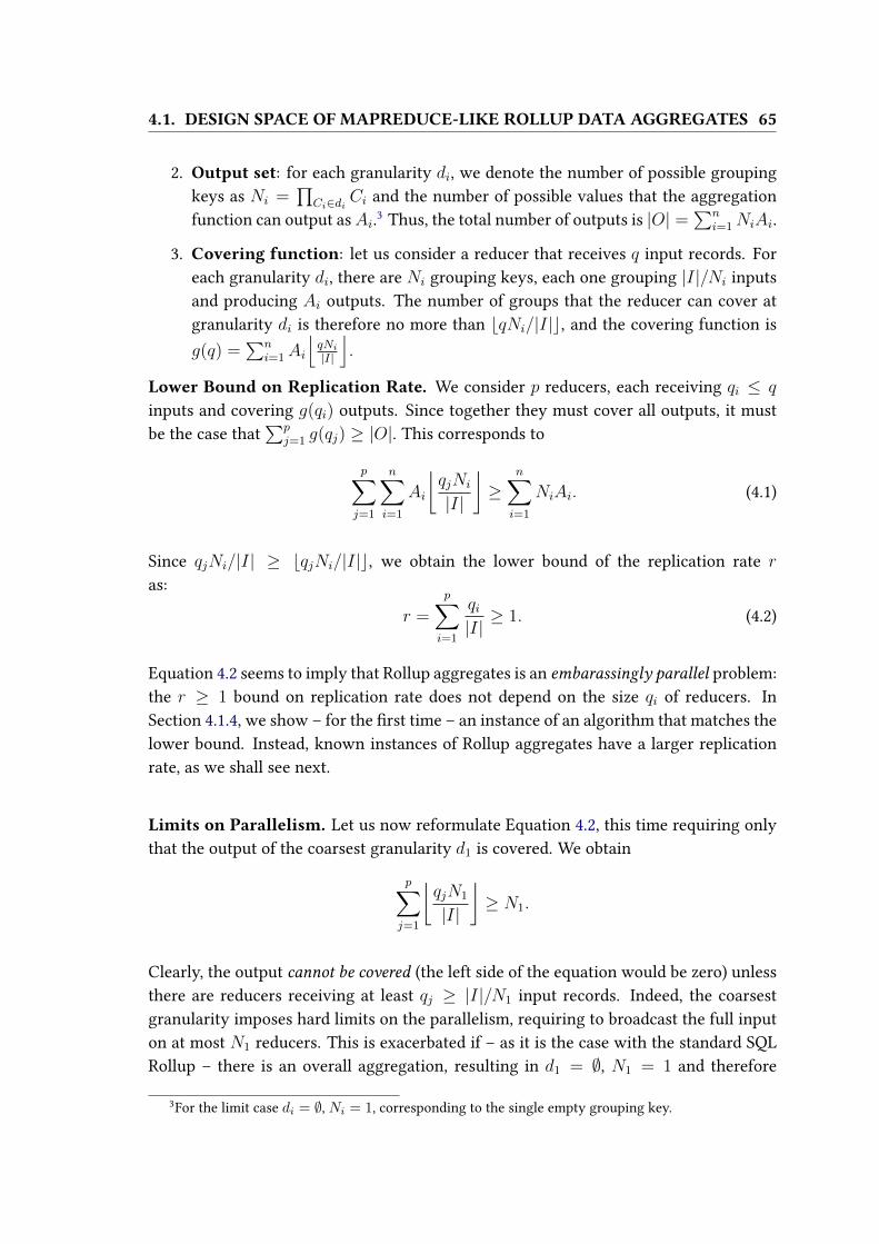
4.1. DESIGN SPACE OF MAPREDUCE-LIKE ROLLUP DATA AGGREGATES 65
2. Output set: for each granularity di, we denote the number of possible grouping
keys as Ni =∏
Ci∈di Ci and the number of possible values that the aggregation
function can output asAi.3
Thus, the total number of outputs is |O| =∑n
i=1NiAi.
3. Covering function: let us consider a reducer that receives q input records. For
each granularity di, there are Ni grouping keys, each one grouping |I|/Ni inputs
and producing Ai outputs. The number of groups that the reducer can cover at
granularity di is therefore no more than bqNi/|I|c, and the covering function is
g(q) =∑n
i=1Ai
⌊qNi|I|
⌋.
Lower Bound on Replication Rate. We consider p reducers, each receiving qi ≤ q
inputs and covering g(qi) outputs. Since together they must cover all outputs, it must
be the case that
∑pj=1 g(qj) ≥ |O|. This corresponds to
p∑j=1
n∑i=1
Ai
⌊qjNi
|I|
⌋≥
n∑i=1
NiAi. (4.1)
Since qjNi/|I| ≥ bqjNi/|I|c, we obtain the lower bound of the replication rate r
as:
r =
p∑i=1
qi|I|≥ 1. (4.2)
Equation 4.2 seems to imply that Rollup aggregates is an embarassingly parallel problem:
the r ≥ 1 bound on replication rate does not depend on the size qi of reducers. In
Section 4.1.4, we show – for the �rst time – an instance of an algorithm that matches the
lower bound. Instead, known instances of Rollup aggregates have a larger replication
rate, as we shall see next.
Limits on Parallelism. Let us now reformulate Equation 4.2, this time requiring only
that the output of the coarsest granularity d1 is covered. We obtain
p∑j=1
⌊qjN1
|I|
⌋≥ N1.
Clearly, the output cannot be covered (the left side of the equation would be zero) unless
there are reducers receiving at least qj ≥ |I|/N1 input records. Indeed, the coarsest
granularity imposes hard limits on the parallelism, requiring to broadcast the full input
on at most N1 reducers. This is exacerbated if – as it is the case with the standard SQL
Rollup – there is an overall aggregation, resulting in d1 = ∅, N1 = 1 and therefore
3For the limit case di = ∅, Ni = 1, corresponding to the single empty grouping key.

66 CHAPTER 4. PHYSICAL OPTIMIZATION FOR DATA AGGREGATION
qj ≥ |I|. A single reducer needs to receive all the input: it appears that no parallelism
whatsoever is possible.
As we show in the following, this negative result however depends on the limitations of
the model: by applying combiners and/or multiple rounds of MapReduce computation,
it is indeed possible to compute e�cient Rollup aggregates in parallel.
Maximum Achievable Parallelism. Our model considers parallelism as determined
by the number of reducers p and the number of input records qj each of them processes.
However, one may also consider the number of output records produced by each reducer:
in that case, the maximum parallelism achievable is when each reducer produces at most
a single output value. This can be obtained by assigning each grouping key in each
granularity to a di�erent reducer; the aggregation function is then guaranteed to output
only one of the Ai possible values. This, however, implies a replication rate r = n; an
implementation of the idea is described in the following section.
4.1.4.2 Baseline algorithms
Next, we de�ne two baseline algorithms to compute Rollup aggregates: Vanilla, which is
discussed in [69], and In Reducer Grouping, which is our contribution. Then, we propose
a hybrid approach that combines both baseline techniques.
Vanilla Approach.
We describe here an approach that maximizes parallelism at the detriment of communi-
cation cost; since this is the approach which is currently implemented in Apache Pig [67]
we refer to it as Vanilla. Nandi et al. [69] refer to it as “naive”.
The Rollup operator can be considered as the result multiple Group By operations: each
of them is carried out at a di�erent granularity. Thus, to perform Rollup on n granular-
ities, for each record, the vanilla approach generates exactly n records corresponding to
these n grouping sets (each grouping sets belongs to one granularity). For instance, tak-
ing as input the (2012, 3, 14, 1) record of the running example, this approach
generates 4 records as outputs of the map phase:
(2012, 3, 14, 1) (day granularity)(2012, 3, *, 1) (month granularity)(2012, *, *, 1) (year granularity)( *, *, *, 1) (overall granularity)
The Reduce step performs exactly as the reduce step of a Group By operation, using the
�rst three records (year, month, day) as keys. By doing this, reducers pull all the data
that is needed to generate each output record (shu�e step), and compute the aggregate

4.1. DESIGN SPACE OF MAPREDUCE-LIKE ROLLUP DATA AGGREGATES 67
(2012, 3, 14, 1)
(2012, 12, 5, 2)
<(2012, 3, 14), 1>
<(2012, 12, 5), 2>
<(2012, 3, *), 1>
<(2012, 12, *), 2>
<(2012, *, *), 1>
<(2012, *, *), 2>
<( *, *, *), 1>
<( *, *, *), 2>
<(2012, 3, 14), 1>
<(2012, 12, 5), 2>
<( *, *, *), 1>
<( *, *, *), 2>
<(2012, *, *), 1>
<(2012, *, *), 2>
<(2012, 3, *), 1>
<(2012, 12, *), 2>
Reducer 1
Reducer 2
Mappers Shuffle
Figure 4.1: Example for the vanilla approach.
(reduce step). Figure 4.1 illustrates a walk-through example of the vanilla approach with
just 2 records.
Parallelism and Communication Cost. The �nal result of Rollup is computed in a single
MapReduce job. As discussed above, this implementation obtains the maximum possible
degree of parallelism, since it can be parallelized up to a level where a single reducer is
responsible of a single output value. On the other hand, this algorithm requires maximal
communication costs, since for each input record, n map output records are generated.
In addition, when the aggregation operation is algebraic [64], redundant computation is
carried out in the reduce phase, since results computed for �ner granularities cannot be
reused for the coarser ones.
Impact of Combiners. This approach largely bene�ts from combiners whenever they are
available, since they can compact the output computed at the coarser granularity (e.g.,in the example the combiner is likely to compute a single per-group value at the yearand overall granularity). Without combiners, a granularity such as overall would result
in shu�ing data from every input tuple to a single reducer.
While combiners are very important to limit the amount of data sent along the network,
the large amount of temporary data generated with this approach is still problematic:
map output tuples need to be bu�ered in memory, sorted, and eventually spilled to disk
if the amount of generated data does not �t in memory. This results, as we show in
Section 4.1.5, in performance costs that are discernible even when combiners are present.

68 CHAPTER 4. PHYSICAL OPTIMIZATION FOR DATA AGGREGATION
(2012, 3, 14, 1)
(2012, 12, 5, 2)
Reducer IRGMappers Shuffle
(2012, 12, 30, 3)
(2013, 5, 24, 4)
<(2012, 3, 14), 1>
<(2012, 12, 5), 2>
<(2012, 12, 30), 3>
<(2013, 5, 24), 4>
<(2012, 3, 14), 1>
<(2012, 12, 5), 2>
<(2012, 12, 30), 3>
<(2013, 5, 24), 4>
<(2012, 3, *), 1>
<(2012, 12, *), 5>
<(2012, *, *), 6>
<(2013, 5, *), 4>
<(2013, *, *), 4>no more input
<( *, *, *), 10>
Figure 4.2: Example for the IRG approach.
In-Reducer Grouping. After analyzing an approach that maximizes parallelism, we
now move to the other end of the spectrum and design an algorithm that minimizes
communication costs. In contrast to the Vanilla approach, where the complexity resides
on the Map phase and the Reduce phase behaves as if implementing an ordinary Group
By clause, we propose an In-Reducer Grouping (IRG) approach, where all the logic of
grouping is performed in the Reduce phase.
In-Reducer Grouping makes use of the possibility to de�ne a partitioner in Hadoop [60,
75]. The mapper selects the columns of interest (in our example, all columns are needed,
so the map function is simply the identity function). The keys are the �nest granularity
dn (day in our example) but data is partitioned only by the columns of the coarsest gran-
ularity d1. In this way, we can make sure that 1) each reducer receives enough data to
compute the aggregation function even for the coarsest granularity d1; 2) the intermedi-
ate keys are sorted [60, 75], so for every grouping key of any granularity di, the reducer
will process consecutively all records pertaining to the given grouping key.
Figure 4.2 shows an example of the IRG approach. The mapper is the identity function,
producing (year, month, day) as the keys and payload as the value. The coarsest granu-
larity d1 is overall, and N1 = 1: hence, all 〈key, value〉 pairs are sent to a single reducer.
The reducer groups all values of the same key, and processes the list of values associated
to that key, thus computing the sum of all values as the total payload t. The grouping
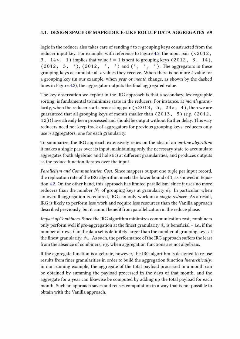
4.1. DESIGN SPACE OF MAPREDUCE-LIKE ROLLUP DATA AGGREGATES 69
logic in the reducer also takes care of sending t to n grouping keys constructed from the
reducer input key. For example, with reference to Figure 4.2, the input pair (<2012,3, 14>, 1) implies that value t = 1 is sent to grouping keys (2012, 3, 14),
(2012, 3, *), (2012, *, *) and (*, *, *). The aggregators in these
grouping keys accumulate all t values they receive. When there is no more t value for
a grouping key (in our example, when year or month change, as shown by the dashed
lines in Figure 4.2), the aggregator outputs the �nal aggregated value.
The key observation we exploit in the IRG approach is that a secondary, lexicographic
sorting, is fundamental to minimize state in the reducers. For instance, at month granu-
larity, when the reducer starts processing pair (<2013, 5, 24>, 4), then we are
guaranteed that all grouping keys of month smaller than (2013, 5) (e.g. (2012,12)) have already been processed and should be output without further delay. This way
reducers need not keep track of aggregators for previous grouping keys: reducers only
use n aggregators, one for each granularity.
To summarize, the IRG approach extensively relies on the idea of an on-line algorithm:
it makes a single pass over its input, maintaining only the necessary state to accumulate
aggregates (both algebraic and holistic) at di�erent granularities, and produces outputs
as the reduce function iterates over the input.
Parallelism and Communication Cost. Since mappers output one tuple per input record,
the replication rate of the IRG algorithm meets the lower bound of 1, as showed in Equa-
tion 4.2. On the other hand, this approach has limited parallelism, since it uses no more
reducers than the number N1 of grouping keys at granularity d1. In particular, when
an overall aggregation is required, IRG can only work on a single reducer. As a result,
IRG is likely to perform less work and require less resources than the Vanilla approach
described previously, but it cannot bene�t from parallelization in the reduce phase.
Impact of Combiners. Since the IRG algorithm minimizes communication cost, combiners
only perform well if pre-aggregation at the �nest granularity dn is bene�cial – i.e., if the
number of rows L in the data set is de�nitely larger than the number of grouping keys at
the �nest granularity,Nn. As such, the performance of the IRG approach su�ers the least
from the absence of combiners, e.g. when aggregation functions are not algebraic.
If the aggregate function is algebraic, however, the IRG algorithm is designed to re-use
results from �ner granularities in order to build the aggregation function hierarchically:
in our running example, the aggregate of the total payload processed in a month can
be obtained by summing the payload processed in the days of that month, and the
aggregate for a year can likewise be computed by adding up the total payload for each
month. Such an approach saves and reuses computation in a way that is not possible to
obtain with the Vanilla approach.

70 CHAPTER 4. PHYSICAL OPTIMIZATION FOR DATA AGGREGATION
overall: d1 year: d2 month: d3 day: d4
P=1 P=2 P=3 P=4
Selected
pivot position
Vanilla-
approach
IRG-approach
Figure 4.3: Pivot position example.
Hybrid approach: Vanilla + IRG. We have shown that Vanilla and IRG are two “ex-
treme” approaches: the �rst one maximizes parallelism at the expense of communication
cost, the second one instead minimizes communication cost but does not provide good
parallelism guarantees.
Neither approach is likely to be an optimal choice for such a tradeo�: in a realistic sys-
tem, we are likely to have way less reducers than number of output tuples to generate
(therefore making the extreme parallelism guarantees produced by Vanilla excessive);
however, in particular when an overall aggregate is needed, it is reasonable to require
an implementation that does not have the bottleneck of a single reducer.
In order to bene�t at once from an acceptable level of parallelism and lower commu-
nication overheads, we propose an hybrid algorithm that �xes a pivot granularity P :
all aggregate functions on granularities between dP and dn are computed using the IRG
algorithm, while aggregates for granularities above dP are obtained using the Vanilla ap-
proach. A choice of P = 1 is equivalent to the IRG algorithm, while P = n corresponds
to the Vanilla approach.
Let us consider again our running example, and �x the pivot position at P = 3, as shown
in Figure 4.3. This choice implies that aggregates for the overall and year granularities
d1, d2 are computed using the Vanilla approach, while aggregates for the other granu-
larities d3, d4 (month and day) are obtained using the IRG algorithm. For example, for
the (2012, 3, 14, 1) tuple, the hybrid approach produces three output records
at the mapper:
(2012, 3, 14, 1) (day granularity)(2012, *, *, 1) (year granularity)( *, *, *, 1) (overall granularity)
In this case the map output key space is partitioned by the month granularity, so that
there is 1) one reducer per each month in the input dataset, that computes aggregates
for granularities up to the month level, and 2) multiple reducers that compute aggre-

4.1. DESIGN SPACE OF MAPREDUCE-LIKE ROLLUP DATA AGGREGATES 71
Reducer 2
(2012, 3, 14, 1)
(2012, 12, 5, 2)
<(2012, 3, 14), 1>
<(2012, 12, 5), 2>
<(2012, *, *), 1>
<(2012, *, *), 2>
<( *, *, *), 1>
<( *, *, *), 2>
<(2012, 3, 14), 1>
<(2012, 12, 5), 2>
<( *, *, *), 1>
<( *, *, *), 2>
<(2012, *, *), 1>
<(2012, *, *), 2>
Reducer 1Mappers Shuffle
<(2012, 3, 14), 1>
<(2012, 3, *), 1>
<( *, *, *), 3>
<(2012, 12, 5), 2>
<(2012, 12, *), 2>
<(2012, *, *), 3>
Figure 4.4: Example for the Hybrid Vanilla + IRG approach.
gates for the overall and year granularities. Figure 4.4 illustrates an example with two
reducers.
Some remarks are in order. Assuming a uniform distribution of the input dataset, the load
on reducers of type 1) is expected to be evenly shared, as an input partition corresponds
to an individual month and not the whole dataset. The load on reducers of type 2) might
seem still prohibitive; however, we note that when combiners are in place they are going
to vastly reduce the amount of data sent to the reducers responsible of the overall and
year aggregate computation. For our example, the reducers of type 2) receive few input
records, because the overall and year aggregates can be largely computed in the map
phase. Furthermore, we remark that the e�ciency of combiners in reducing input data to
reducers (and communication costs) is very high for coarse granularities, and decreases
towards �ner granularities: this is why the IRG algorithm applies the Vanilla approach
from the pivot position, up to coarse granularities.
Parallelism and Communication Cost. The performance of the hybrid algorithm depends
on the choice of P : the replication rate (before combiners) is P . The number of reducer
that this approach can use is the total of 1) NP grouping keys that are handled with
the IRG algorithm, and 2)∑P−1
i=0 Ni grouping keys that are handled with the Vanilla
approach. Ideally, an a priori knowledge of the input data can be used to guide the
choice of the pivot position. For example, if the data in our running example is known
to span over tens of years and we know we only have ten reducer slots available (i.e., at
most ten reducer tasks can run concurrently), a choice of partitioning by year (P = 2)
would be reasonable. Conversely, if the dataset only spans a few years and hundreds of
reducer slots are available, then it would be better to be more conservative and choose

72 CHAPTER 4. PHYSICAL OPTIMIZATION FOR DATA AGGREGATION
Reducer 1
Reducer 2
(2012, 3, 14, 1)
(2012, 12, 5, 2)
<(2012, 3, 14), 1>
<(2012, 12, 5), 2>
<(2012, *, *), 1>
<(2012, *, *), 2>
<(2012, 3, 14), 1>
<(2012, 12, 5), 2>
<(2012, *, *), 1>
<(2012, *, *), 2>
Mappers Shuffle
<(2012, 3, 14), 1>
<(2012, 3, *), 1>
<( *, *, *), 3>
<(2012, 12, 5), 2>
<(2012, 12, *), 2>
<(2012, *, *), 3>
Figure 4.5: Example for the Hybrid IRG + IRG approach.
P = 3 or P = 4 to obtain better parallelism at the expense of a higher communication
cost.
Impact of Combiners. The hybrid approach heavily relies of combiners. Indeed, when
combiners are not available, all input data will be sent to the one reducer in charge of
the overall granularity; in this case, it is then generally better to choose P = 1 and
revert to the IRG algorithm. However, when the combiners are available, the bene�t for
the hybrid approach is considerable, as discussed above.
4.1.4.3 Alternative hybrid algorithms
We now extend the hybrid approach we introduced previously, and propose two alter-
natives: a single job involving two parallel IRG instances, and a chained job involving a
�rst IRG computation and a �nal IRG aggregation.
Hybrid approach: IRG + IRG. In the previous section, we have shown that it is pos-
sible to design an algorithm aiming at striking a good balance between parallelism and
replication rate, using a single parameter, i.e. the pivot position. In the baseline hybrid
approach, parallelism is an increasing function of the replication rate, so that better par-
allelism is counterbalanced by higher communication costs in the shu�e phase.
Here, we propose an alternative approach that results in a constant replication rate of 2:
the “trick” is to replace the Vanilla part of the baseline hybrid algorithm with a second
IRG approach. Using the same running example as before, for the tuple (2012, 3,14, 1), and selecting the pivot position P = 3, the two map output records are:
(2012, 3, 14, 1) (day granularity)(2012, *, *, 1) (year granularity)

4.1. DESIGN SPACE OF MAPREDUCE-LIKE ROLLUP DATA AGGREGATES 73
Figure 4.5 on the facing page illustrates a running example. In this case, the map out-
put key space is partitioned by the month granularity, such that there is one reducer
per month that uses the IRG algorithm to compute aggregates; in addition, there is onereducer receiving all tuples having ALL values taking care of the year and overall gran-
ularities, using again the IRG approach. As before, the role of combiners is crucial: the
amount of (year, *, *, payload) tuples that are sent to the single reducer taking
care of year and overall aggregates is likely to be very small, because opportunities to
compute partial aggregates in the map phase are higher for coarser granularities.
Parallelism and Communication Cost. This algorithm has a constant replication rate of 2.
As we show in Section 4.1.5, the choice of the pivot position P is here much less decisive
than for the baseline hybrid approach: this can be explained by the fact that moving the
pivot to �ner granularities does not increase communication costs, as long as the load
on the reducer taking care of the aggregates for coarse granularities remains low.
Impact of Combiners. Similarly to the baseline hybrid approach, this algorithm relies
heavily on combiners; if combiners are not available, then, a simple IRG approach
would be preferable.
Chained IRG. It is possible to further decrease the replication rate and hence the com-
munication costs of computing Rollup aggregates by adopting a multi-round approach
composed of two chained MapReduce jobs. In this case, the �rst job pre-aggregates
results up to the pivot position P using the IRG algorithm; the second job uses partial
aggregates from the �rst job to produce – on a single reducer – the �nal aggregate result,
again using IRG. We note here that a similar observation, albeit for computing matrix
multiplication, is also discussed in detail in [49].
Parallelism and Communication Cost. The parallelism of the �rst MapReduce job is deter-
mined by the amount NP of grouping keys at the pivot position; the second MapReduce
job, has a single reducer. However, the input size of the second job is likely to be orders
of magnitude smaller than the �rst one, so that the runtime of the reduce phase of the
second job – unless the pivot position puts too much e�ort on the second job – is gen-
erally negligible. The fact that the second reducer operates on a very small amount of
input, results in a replication rate very close to 1.
The main drawback of the chained approach is due to job scheduling strategies: if jobs
are scheduled in a system with idle resources, as we show in Section 4.1.5, the chained
IRG algorithm results in the smallest runtime. However, in a loaded system, the sec-
ond (and in general very small) MapReduce job could be scheduled later, resulting in
arti�ciously large delays between job submission and its execution.

74 CHAPTER 4. PHYSICAL OPTIMIZATION FOR DATA AGGREGATION
Impact of Combiners. This approach does not rely heavily on combiners per se. However,
it requires the aggregation function to be algebraic in order to make it possible for the
second MapReduce job to re-use partial results.
4.1.5 Experimental Evaluation
We now proceed with an experimental approach to study the performance of the algo-
rithms we discussed in this work. We use two main metrics: runtime – i.e. job execution
time – and total amount of work, i.e. the sum of individual task execution times. Runtime
is relevant on idle systems, in which job scheduling does not interfere with execution
times; total amount of work is instead an important metric to study in heavily loaded
systems where spare resources could be assigned to other pending jobs.
4.1.5.1 Experimental Setup
Our experimental evaluation is done on a Hadoop cluster of 20 slave machines (8GB
RAM and a 4-core CPU) with 2 map and 1 reduce slot each. The HDFS block size is set
to 128MB. All results shown in the following are the average of 5 runs: the standard
deviation is smaller than 2.5%, hence – for the sake of readability – we omit error bars
from our �gures.
We compare the �ve approaches described in Section 4.1.4: baseline algorithms (Vanilla,
IRG, Hybrid Vanilla + IRG) and alternative hybrid approaches (Hybrid IRG + IRG
Chained IRG). We evaluate a single Rollup aggregation job over (overall, year, month,
day, hour, minute, second) that uses the SUM aggregate function which, being algrebraic,
can bene�t from combiners. Our input dataset is a synthetic log-trace representing his-
torical tra�c measurements taken by an Internet Service Provider (ISP): each record in
our log has 1) a time-stamp expressed in (year, month, day, hour, minute, second); and 2)a number representing the payload (e.g. number of bytes sent or received over the ISP
network). The time-stamp is generated uniformly at random within a variable number
of years (where not otherwise speci�ed, the default is 40 years). The payload is a uni-
formly random positive integer. Overall, our dataset comprises 1.5 billion binary tuples
of size 32 bytes each, packed in a SequenceFile [75].
4.1.5.2 Results
This section presents a range of results we obtained in our experiments. Before delving
into a comparative study of all the approaches outlined above, we �rst focus on studying
the impact of combiners on the performance of the Vanilla approach. Then, we move
to a detailed analysis of runtime and amount of work for baseline algorithms (Vanilla,

4.1. DESIGN SPACE OF MAPREDUCE-LIKE ROLLUP DATA AGGREGATES 75
Figure 4.6: Impact of combiners on runtime for the Vanilla approach.
IRG, and Hybrid), and we conclude with an overview to outline merits and drawbacks
of alternative hybrid approaches.
The role of combiners. Figure 4.6 illustrates a break-down of the runtime for
computing the Rollup aggregate on our dataset, showing the time a job spend in the
various phases of a MapReduce computation. Clearly, combiners play an important role
for the Vanilla approach: they are bene�cial in the shu�e and reduce phases. When
combiners cannot be used (e.g. because the aggregation function is not algebraic),
the IRG algorithm outperforms the Vanilla approach. With combiners enabled, the
IRG algorithm is slower (larger runtimes) than the Vanilla approach: this can be
explained by the lack of parallelism that characterizes IRG, wherein a single reducer is
used as opposed to 20 reducers for the Vanilla algorithm. Note that, in the following
experiments, combiners are systematically enabled. Finally, Figure 4.6 con�rms that
the IRG approach moves algorithmic complexity from the map phase to the reduce phase.
Baseline algorithms. In Figure 4.7 we compare the runtime of Vanilla, IRG, and the
hybrid Vanilla + IRG approach. In our experiments we study the impact of the pivot
position P , in lights of the “nature” of the input dataset: we synthetically generate data
such that they span 1, 10 and 40 years worth of tra�c logs.4
Clearly, IRG (which corresponds to P = 1) is the slowest approach in terms of run-
time. Indeed, using a single reducer incurs in prohibitive I/O overheads: the amount of
4Note that the size – in terms of number of tuples – of the input data is kept constant, irrespectively
of the number of represented years.

76 CHAPTER 4. PHYSICAL OPTIMIZATION FOR DATA AGGREGATION
IRG (P=1) P=2 P=3 P=4 P=5 P=6 Vanilla (P=7)0
1000
2000
3000
4000
5000
Ru
ntim
e (
se
co
nd
s)
40 years
10 years
1 years
Figure 4.7: Runtime comparison of baseline approaches.
data shu�ed into a single reducer is too large to �t into memory, therefore spilling and
merging operations at the reducer proceed at disk speeds. Although no redundant com-
putations are carried out in IRG, I/O costs outweigh the savings in computations.
A hybrid approach (2 ≤ P ≤ 6) outperforms both IRG and Vanilla algorithms, with
runtime as little as half that of the Vanilla approach. Communication costs make the
runtime grow slowly as the pivot position moves towards �ner granularities, suggesting
that in doubt, it is better to position the pivot to the right (increased communication
costs) rather than to the left (lack of parallelism). In our case, where a maximum of 20
reduce tasks can be scheduled at any time, our results indicate that P should be chosen
such that NP is larger than the number of available reducers. As expected, experiments
with data from a single year indicate that the pivot position should be placed further to
the right: the hybrid approach with P = 2 essentially performs as badly as the single-
reducer IRG.
Now, we present our results under a di�erent perspective: we focus on the total amountof work executed by a Rollup aggregate implemented according to our baseline algo-
rithms. We de�ne the total amount of work for a given job as the sum of the runtime of
each of its (map and reduce) tasks. Figure 4.8 indicates that the IRG approach consumes
the least amount of work. By design, IRG is built to avoid redundant work: it has mini-
mal replication rate, and the single reducer can produce Rollup aggregates with a single
pass over its input.
As a general remark, that applies to all baseline algorithms, we note that the total amount
of work is largely determined by the map phase of our jobs. The trend is tangible as P
moves toward �ner granularities: despite communication costs (the shu�e phase, which
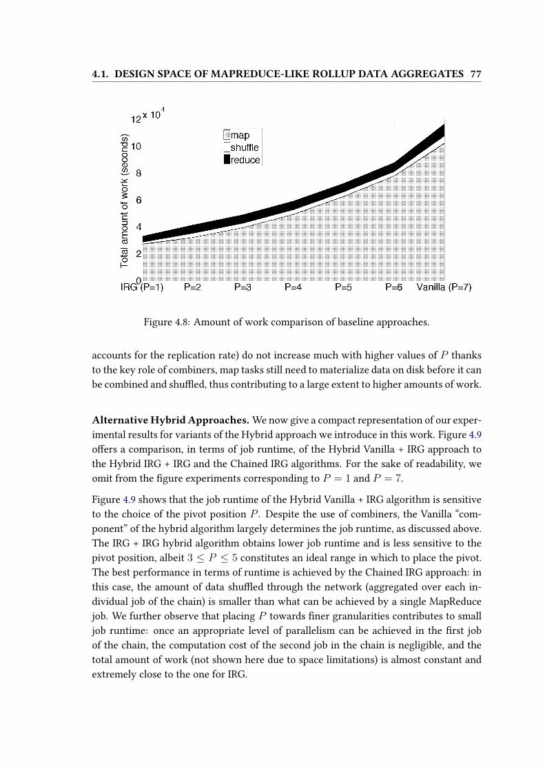
4.1. DESIGN SPACE OF MAPREDUCE-LIKE ROLLUP DATA AGGREGATES 77
Figure 4.8: Amount of work comparison of baseline approaches.
accounts for the replication rate) do not increase much with higher values of P thanks
to the key role of combiners, map tasks still need to materialize data on disk before it can
be combined and shu�ed, thus contributing to a large extent to higher amounts of work.
AlternativeHybrid Approaches. We now give a compact representation of our exper-
imental results for variants of the Hybrid approach we introduce in this work. Figure 4.9
o�ers a comparison, in terms of job runtime, of the Hybrid Vanilla + IRG approach to
the Hybrid IRG + IRG and the Chained IRG algorithms. For the sake of readability, we
omit from the �gure experiments corresponding to P = 1 and P = 7.
Figure 4.9 shows that the job runtime of the Hybrid Vanilla + IRG algorithm is sensitive
to the choice of the pivot position P . Despite the use of combiners, the Vanilla “com-
ponent” of the hybrid algorithm largely determines the job runtime, as discussed above.
The IRG + IRG hybrid algorithm obtains lower job runtime and is less sensitive to the
pivot position, albeit 3 ≤ P ≤ 5 constitutes an ideal range in which to place the pivot.
The best performance in terms of runtime is achieved by the Chained IRG approach: in
this case, the amount of data shu�ed through the network (aggregated over each in-
dividual job of the chain) is smaller than what can be achieved by a single MapReduce
job. We further observe that placing P towards �ner granularities contributes to small
job runtime: once an appropriate level of parallelism can be achieved in the �rst job
of the chain, the computation cost of the second job in the chain is negligible, and the
total amount of work (not shown here due to space limitations) is almost constant and
extremely close to the one for IRG.

78 CHAPTER 4. PHYSICAL OPTIMIZATION FOR DATA AGGREGATION
P=2 P=3 P=4 P=5 P=60
500
1000
1500
2000
2500
3000
3500
4000
Ru
ntim
e (
se
co
nd
s)
Hybrid Vanilla+IRG
Hybrid IRG+IRG
Chained IRG
Figure 4.9: Comparison between alternative hybrid approaches.
We can now summarize our �ndings as follows:
• All the approaches that we examined greatly bene�t from the, fortunately com-
mon, property that aggregation functions are algebraic and therefore enable com-
biners and re-using partial results. If this is not the case, approaches based on the
IRG algorithm are preferable.
• If total amount of work is the metric to optimize, IRG is the best solution because
it minimizes redundant work. If low latency is also required, hybrid approaches
o�er a good trade-o�, provided that the pivot position P is chosen appropriately.
• Our alternative hybrid approaches are the best performing solutions; both are very
resilient to bad choices of theP pivot position, which can therefore be chosen with
a very rough a-priori knowledge of the input dataset. Chained IRG provides the
best results due to its minimal communication costs. However, chained jobs may
su�er from bad scheduling decisions in a heavily loaded cluster, as the second job
in the chain may “starve” due to large jobs being scheduled �rst. The literature on
MapReduce scheduling o�ers solutions to this problem [27].

4.2. EFFICIENT AND SELF-BALANCED ROLLUP OPERATOR FORMAPREDUCE-LIKE SYSTEMS 79
4.2 E�cient and Self-Balanced Rollup Operator forMapReduce-like Systems
4.2.1 Introduction
Despite the importance of data aggregation, the �eld of large-scale data-intensive com-
puting systems – where data can reach petabytes and be distributed on clusters of thou-
sands of nodes – has not seen much e�ort toward e�cient implementations of the above
concepts. In the Hadoop MapReduce ecosystem [1,60], high-level query languages such
as Pig Latin [8] and HiveQL [7] o�er simple implementations of the above constructs,
which do not perform aggressive optimizations. In enterprise workloads, jobs coming
from queries written in high-level languages are the majority [71]; an optimized imple-
mentation of these operators is therefore truly desirable.
Our work in the previous Section 4.1 proposes several e�cient physical algorithms for
MapReduce-like Rollup. In this Section, we focus on the design and implementation of
a light-weight, cost-based optimization module for Rollup for high-level languages. We
call this module: a Rollup operator.
Existing implementations are not satisfying: as we discuss in Section 4.2.2, current
Rollup algorithms are naively biased toward extreme levels of parallelism. As a con-
sequence, these approaches trade a theoretical possibility of scaling several orders of
magnitude beyond the scale attainable by real-world clusters with a very signi�cant
overhead in terms of communications.
There are alternative Rollup algorithms (Section 4.1) that allow tuning the level of paral-
lelism and the communication overhead of their implementation: with a proper setting,
these algorithms perform better than naive implementations. Such approaches are ap-
pealing in the abstract, but they are practically very di�cult for users to apply, since to
determine the proper setting, they would require users to know: (i) the internals of the
algorithm’s implementation; (ii) statistical information about data distribution; (iii) size
and performances of the cluster on which the algorithm is implemented. These require-
ments are di�cult to meet at once, and they are essentially prohibitive in the context of
high-level languages, whose very reason of existence is to hide this kind of complexities
and allowing users to concentrate on extracting meaning from data.
As a result, in this Section, we design (in Section 4.2.3) and implement a new Rollup
operator that is completely transparent to users. Our operator automatically collects
statistics about data and cluster performance. Subsequently it uses this information to:
(i) balance load across di�erent nodes in the cluster; (ii) determine an appropriate oper-
ation point of Rollup algorithms using a lightweight cost-based optimizer.

80 CHAPTER 4. PHYSICAL OPTIMIZATION FOR DATA AGGREGATION
We perform an extensive experimental campaign (Section 4.2.5) to assess the validity
of our design choices, using both real and synthetic datasets, and comparing the per-
formance of a variety of di�erent Rollup algorithms. Results indicate that our Rollup
operator, that relies on automatically tuned algorithms, delivers superior performance
when compared to current Rollup implementations for the Apache Pig system. Our
operator is released as open source software5, and is currently in the process of being
integrated in the upstream Apache Pig Latin language implementation. We summarize
this work in Section 4.4.
4.2.2 Preliminaries & Related Work
E�cient computation of data summaries is an important topic that has received wide
attention by the database community. Recently, such interest has led to several works
to bring the bene�ts of data aggregation to MapReduce systems as well.
In this Section, we review several Rollup algorithms, for both traditional databases and
MapReduce systems, and motivate the need for a substantially di�erent approach. Rollup
is a data operator �rst introduced by Gray et al. [64] as a special case of Cube. The Rollup
operator aggregates data along a dimension by “climbing up” the dimension hierarchy.
For example, to aggregate the volume of cars sold in the last several years, it is possible
to use the Rollup operator to obtain sales along the time dimension, including multi-
ple levels: total, year, month, and day. These levels form a hierarchy, of which
total is the top level that includes aggregates from all records.
4.2.2.1 Rollup in Parallel Databases
Traditionally, the Rollup operator was studied through the lenses of its generalized op-
erator, Cube, that groups data along all combinations (called views) of di�erent levels in
hierarchies. In Rollup, a view is equivalent to a level of the rollup hierarchy. In our car
sales example, we have 4 di�erent views.
Harinaryan et al. [66] introduced a model to evaluate the cost of executing Cube and
a greedy algorithm to select a near-optimal execution plan. Agarwal et al. [51] pro-
posed top-down algorithms (PipeSort, PipeHash) to optimize Cube computation: using
�ner group-bys to compute coarser ones (i.e. using month to compute year). Beyer
and Ramakrishnan [58] suggested a bottom-up computation (BUC) to construct results
from coarser to �ner group-bys by reusing as much as possible the previously com-
puted sort orders. All of these works are sequential algorithms which focus on single
servers.
5h�ps://bitbucket.org/bigfootproject/rollupmr

4.2. EFFICIENT AND SELF-BALANCED ROLLUP OPERATOR FORMAPREDUCE-LIKE SYSTEMS 81
Scalable algorithms to handle the Rollup and Cube operators in parallel databases also
received considerable attention. They are divided into two main groups: work partition-ing [37,48] and data partitioning [45,46]. In work partitioning, each processor (or node)
of the cluster computes aggregates for a set of one or many views independently. To
do that, all processors access concurrently the entire dataset. Typically such an access
is o�ered by a shared-disk array that is both expensive and di�cult to scale in term of
performance and size. Instead, data partitioning algorithms divide the input data set into
various subsets. A node computes all views associated to the subsets of data it hosts. To
obtain global aggregates, a subsequent merge phase is required. The main advantage of
such a Two Phase algorithm is that nodes need not to have access to the whole data set
but work on a small portion that can be easily stored on local memory/disks.
4.2.2.2 Rollup in MapReduce
In what follows, we assume the reader to be familiar with the MapReduce paradigm and
its well-known open-source implementation Hadoop [60, 75].
Currently, MapReduce high-level languages such as Apache Pig and Hive borrow from
parallel databases the Two Phase algorithm described previously. Its MapReduce vari-
ant is straightforward: each mapper computes aggregates of the whole Rollup hierarchy
from its local data, then sends the partial results to reducers which merge and return the
�nal aggregates. The MapReduce Two Phase (MRTP) algorithm, which can use combin-
ers as an optimization, produces a large quantity of intermediate data that impose strain
on network resources. In addition, a large number of intermediate data increases notice-
ably mapper overheads to sort and eventually spill them to disk. Similarly, since reducers
compute aggregates in each view separately, the MRTP algorithm presents signi�cant
overheads due to redundant computation.
These overheads are the main reason for the MRTP ine�ciency, and they can be avoided
by employing the in-reducer grouping (IRG) design pattern [80]. IRG computes aggre-
gates in a top-down manner by exploiting custom partitioning and sorting in MapReduce
to move the grouping logic from the shu�e phase to reducers. However, IRG severely
lacks parallelism: all processing is performed by a single reducer.
More recent works explore the design space of one-round MapReduce Rollup algorithms
by studying the trade-o� between communication cost (amount of data sent over net-
work) and parallelism [28]. Through a parameter called pivot position, the Hybrid
IRG+IRG algorithm (HII) provides users with the �exibility of choosing a sweet spot
to balance parallelism and communication cost. For one-round MapReduce algorithms,
the HII algorithm is shown (analytically and experimentally) to achieve the best perfor-
mance, if and only if the pivot position is set to the optimal value. Otherwise, the HII

82 CHAPTER 4. PHYSICAL OPTIMIZATION FOR DATA AGGREGATION
algorithm represent a valid theoretical contribution, albeit impractical to be used as a
baseline for a high-level language operator.
For multi-round MapReduce Rollup algorithms, the work in [28] also proposes the
ChainedIRG algorithm, which splits a Rollup operator into two chained MapReduce jobs
based on a parameter (again, a pivot position). The pivot position divides the Rollup hier-
archy between two jobs. The �rst job computes a subset of the hierarchy and the second
job takes the �rst job’s results to compute the rest.
Finally, MRCube, proposed by Nandi et al. [69], implements Cube and Rollup operators
in three rounds. The �rst round performs record random sampling on input data and es-
timates the cardinality of reducer keys. It serves identifying large groups of keys whose
cardinality exceeds the capacity of a reducer, and set a partition factor N . In the second
round, MRCube splits these large groups into N sub-groups using value partitioning:
two keys belong to the same sub-groups if and only if their values of the aggregated at-
tribute are congruent modulo N . Each sub-group is computed as a partial aggregate by
some reducer using the BUC algorithm [66]. The third round merges partial aggregates
to produce �nal results. As a consequence, reducers do not handle excessive amounts
of data, but the execution plan requires multi-rounds of MapReduce jobs. The authors
also note that the value partitioning may be problematic when data is skewed on the ag-
gregated attribute, as it can create sub-groups that exceed the reducer capacity and slow
down the job. Also, as the number of large-groups may be high, the �rst step of MRCube
can create a signi�cant overhead and make MRCube slower than the MapReduce Two
Phase algorithm [69].
4.2.2.3 Other Related Works
It is well known that MapReduce algorithms may su�er from poor performance if data
is skewed. SkewReduce [53] is a framework that manages data and computation skew
by using user domain knowledge to break the map and reduce tasks into smaller tasks;
then it �nds the optimal partition plan to achieve load balancing. SkewTune [54] is a
dynamic skew mitigation system: by modifying the MapReduce architecture, it detects
stragglers in reducers and pro-actively repartitions the unprocessed data to other idle
reducers. Another approach is to design skew-resistant operators: data skew is handled
at the algorithmic level. This approach does not require additional components, user
interventions or modi�cations to the Hadoop framework. For instance, [56] proposes
an algorithmic approach to handle set-similarity join. Apache Pig also supports a skew-
resistant equi-join operator. For the MapReduce data aggregation, to the best of our
knowledge, our work is the �rst to tackle a skew-resistant Rollup operator.
Finally, we consider related works that use a cost model to �nd optimal execution plans.
SkewReduce [53] uses a cost model that requires two user-supplied cost functions. MR-

4.2. EFFICIENT AND SELF-BALANCED ROLLUP OPERATOR FORMAPREDUCE-LIKE SYSTEMS 83
Share [57] proposes work-sharing optimizations based on a cost model to predict merged
job’s runtime. This model requires users to provide a set of constant, static parameters,
that represent the underlying cluster performance. Both practices are not transparent to
users. The latter is problematic in practice because cluster performance changes over-
time, and in many cases, clusters are dynamically allocated (e.g. Amazon EC2, Google
App Engine) which means unpredictable performance.
Instead, as we show in the next Section, our approach automatically measures cluster
performance. These measurements are fed to a regression model that predicts the Rollup
runtime. This is completely transparent to users, and adaptable to any cluster con�gu-
ration.
4.2.3 A New Rollup Operator
In this Section, we describe our design of an e�cient and skew-resistant Rollup operator.
Our approach can be integrated directly in current MapReduce high-level languages
such as Apache Pig and Hive, and it is completely transparent to users. Our design
avoids any modi�cations to the Hadoop framework or the MapReduce programming
model, thus making our work directly applicable to any MapReduce-like systems. Our
approach can also handle a stateless design (i.e. no historical execution statistics), which
is the current standard practice for systems that provide high-level languages on top of
MapReduce.
4.2.3.1 Rollup Operator Design
Our Rollup operator has two main components: the tuning job and the Rollup query.
The Rollup query can implement one of several Rollup algorithms, such as MRTP, HII,
ChainedIRG, MRCube as described in Section 4.2.2.2. We discuss the choice of an appro-
priate algorithm in Section 4.2.3.2.
The heart of our work is the tuning job, a primary component with two main goals.
The �rst is to determine how to achieve load-balancing taking into account skewed data
when executing the Rollup query, which is clearly bene�cial to any Rollup algorithm.
The second goal is to determine the most suitable operating point of the Rollup query,
provided that the underlying Rollup algorithm requires tuning. For example, Rollup
algorithms like HII and ChainedIRG both rely on an essential parameter that, if not
properly tuned, can lead to ine�cient executions and bad performance. In this case, the
tuning job automatically sets the parameter of such algorithms to the proper value, such
that performance is maximized.
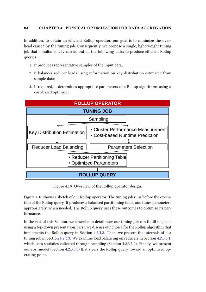
84 CHAPTER 4. PHYSICAL OPTIMIZATION FOR DATA AGGREGATION
In addition, to obtain an e�cient Rollup operator, our goal is to minimize the over-
head caused by the tuning job. Consequently, we propose a single, light-weight tuning
job that simultaneously carries out all the following tasks to produce e�cient Rollup
queries:
1. It produces representative samples of the input data;
2. It balances reducer loads using information on key distribution estimated from
sample data;
3. If required, it determines appropriate parameters of a Rollup algorithms using a
cost-based optimizer.
Figure 4.10: Overview of the Rollup operator design.
Figure 4.10 shows a sketch of our Rollup operator. The tuning job runs before the execu-
tion of the Rollup query. It produces a balanced partitioning table, and tunes parameters
appropriately, when needed. The Rollup query uses these outcomes to optimize its per-
formance.
In the rest of this Section, we describe in detail how our tuning job can ful�ll its goals
using a top-down presentation. First, we discuss our choice for the Rollup algorithm that
implements the Rollup query in Section 4.2.3.2. Then, we present the internals of our
tuning job in Section 4.2.3.3. We examine load balancing on reducers in Section 4.2.3.3.1,
which uses statistics collected through sampling (Section 4.2.3.3.2). Finally, we present
our cost model (Section 4.2.3.3.3) that steers the Rollup query toward an optimized op-
erating point.

4.2. EFFICIENT AND SELF-BALANCED ROLLUP OPERATOR FORMAPREDUCE-LIKE SYSTEMS 85
4.2.3.2 The Rollup Query: Algorithmic Choice
The design of our Rollup operator is generic enough to employ any Rollup algorithm.
However, in this work, we focus on the two algorithms that proved to o�er, consis-
tently, superior performance when compared to alternative approaches, namely the Hy-
brid IRG+IRG (HII) and ChainedIRG [28]. Indeed, unlike MRTP, MRCube and IRG, such
algorithms have the �exibility to adjust the level of parallelism to exploit, which trans-
lates into a much lower communication cost compared to MRTP and MRCube. Previous
results in the literature [28] corroborate our choice, which we con�rm in our extensive
performance evaluation in Section 4.2.5.
Now, both ChainedIRG and HII require a fundamental parameter P called pivot posi-tion. Let us consider the Rollup dimension with n levels: {d1, d2, . . . , dn} in which
d1 is the top-level of the hierarchy. P divides the Rollup dimensions in two subsets:
S1 = {d1, . . . , dP−1} and S2 = {dP , . . . , dn}. Each subset now represents a sub-Rollup
query. The di�erence between ChainedIRG and HII is that, while HII computes each
sub-Rollup query independently and has only one job, ChainedIRG exploits the aggre-
gates on S2 to compute aggregates on S1 (hence, it requires two jobs). Nonetheless, both
algorithms use the IRG design pattern to compute each sub-Rollup query.
Although the experimental results in [28] indicate that ChainedIRG has the best runtime
in an isolated system, in this section we cast our Rollup operator on the HII algorithm
because it is less prone to delays due to scheduling when the cluster is loaded. Instead,
the runtime of multi-phase algorithms (such as ChainedIRG) could be in�ated since the
job scheduler can dedicate resources to other jobs in between the phases. Nonetheless,
we note that our tuning job can easily accommodate alternative algorithms, and we show
this in our experimental evaluation, where we present results of our Rollup operator
with instances of the Rollup query implementing all the algorithms we discussed in
Section 4.2.2.
Continuing our example in Section 4.2.2, if P = 3 the two subsets are {total,year}and {month,day}. For each input record, the map phase of HII generates 2
〈key, value〉 pairs of the bottom level of each subset (i.e. year and day).
Then for each subset, the mappers partition their 〈key, value〉 pairs by the top level of this
subset (i.e. total and month). Taking advantage of this partitioning scheme and the
sorting done by the MapReduce framework, day-to-month and year-to-total aggregates
can be processed independently in the reduce phase. In fact, HII applies a top-down
approach: we compute aggregates for each day in a month; then combine results to
obtain month aggregates. Similarly, we compute results for each year and construct the
total aggregate.
Choosing an appropriate pivot position P is crucial in HII and ChainedIRG, because it
determines the parallelism as well as the communication cost of such algorithms. Values

86 CHAPTER 4. PHYSICAL OPTIMIZATION FOR DATA AGGREGATION
of P that are too high can impose an excessive load on the reducer that is responsible for
the total aggregates, and lessen the bene�t of combiners (i.e. higher communication
cost). Instead, low values of P could result in insu�cient parallelism causing poor load
balancing. Finding the proper value for P is a non-trivial problem.
4.2.3.3 The Tuning Job
We now discuss our main contribution, the tuning job, that balances the reducer load and
�nds the optimal value of P . We propose a novel mechanism that enables a single-round
MapReduce job to collect statistical information about the input data and the underly-
ing cluster performance, determine and impose a load balancing scheme and optimize
the selection of the pivot position for the HII algorithm. The tuning job operates as
follows:
• For each possible pivot position P , we estimate a key distribution: a mapping be-
tween each partitioning key and the number of records that correspond to that
key (i.e. its cardinality).
• For each pivot position, we devise a greedy key partitioning scheme that balances
as much as possible the load between reducers;
• For each pivot position, using performance measurements gathered throughout
the tuning job execution, we use a cost model to predict the runtime associated to
each pivot position. We then select the pivot position that yields the shortest job
runtime.
Because the search space for an optimal pivot position is small and capped by n – the
number of grouping sets – our mechanism can a�ord to evaluate all values of P . We
minimize the overhead of the tuning job by executing it as a single MapReduce job, where
the input data is read only once and all candidate values for P are evaluated in parallel.
The rest of this section presents how each step of our tuning job is accomplished. Key
partitioning described in Section 4.2.3.3.1, uses the estimation of key distribution using
sampling (Section 4.2.3.3.2). From partitioning outputs, we extract the reducer loads to
feed into our cost model, as shown in Section 4.2.3.3.3. The cost model uses a regression-
based approach that predicts the runtime of both mappers and reducers for each value
of P ; this model uses performance measurements that we collect in the tuning job as a
training set.
4.2.3.3.1 Balancing Reducer Load Skewed data motivates the need for reducer
load-balancing. In this step, we balance reducer load using cardinalities of partitioning
keys obtained from the key distribution estimation discussed in Section 4.2.3.3.2. The
input of this step is a set of keys K and an estimation of their respective cardinalities

4.2. EFFICIENT AND SELF-BALANCED ROLLUP OPERATOR FORMAPREDUCE-LIKE SYSTEMS 87
C = {Ck|k ∈ K}. We then perform load balancing by partitioning the keys in K on r
reducers to minimize the input keys on the most loaded reducer. This problem can be
reduced to the multi-way number partitioning problem, which is NP-complete [70]. We
thus opt for a greedy solution: sort all reduce input keys by descending cardinalities, and
assign at each step a key to the least loaded reducer. Our algorithm uses smaller cardi-
nalities to counter the imbalance created by large cardinalities that are allocated �rst. Its
runtime is linear with respect to the number of keys. Thanks to the role of combiners,
the number of input records sent to each reducer is quite small; for this reason, as we
shall see in Section 4.2.5.2, our load balancing strategy is very e�ective in practice.
The output of this greedy algorithm is a reducer partitioning table, which we broadcast to
all mappers to determine the key-reducer mapping. When the Rollup query is running,
such a partitioning is kept in a hash table and used to “route” keys to reducers. If, due
to sampling, a key does not appear in the hash table, it is “routed” to a pseudo-random
reducer using hashing. We note that the impact of such missing keys is minimal on load
balancing, as they correspond to infrequent input data.
4.2.3.3.2 Sampling and Computing Key Distribution The load balancing step
we just discussed requires the number of reducer input records per grouping key, i.e.its cardinality. Without modifying the MapReduce architecture, we cannot count these
cardinalities on the �y when processing data. Instead, we resort to sampling: we only
read data from a small subset of the input data, and we gather key distributions and
cardinalities that are the input of the load balancing step. These steps are counted as an
overhead in our total job runtime.
In MapReduce, uniform record random sampling from the whole input would be inef-
�cient, as it requires the whole data to be read and parsed. Instead, we employ chunkrandom sampling. Chunk sampling allows low overhead, as it reads a very small por-
tion of input data. The dataset is split in chunks of data that have di�erent sizes: this is
also useful for the linear regression model we describe in Section 4.2.3.3.5. Each chunk is
chosen with probability σ, a parameter we explore in our experimental evaluation.
However, chunk sampling introduces sampling bias. To reduce this bias, for each chunk,
we output each record only once, regardless of its multiple appearances in that chunk.
Such a technique can be easily achieved by using combiners. In the reducers, we collect
records from di�erent chunks and treat them like records gathered from uniform random
sampling. This method, albeit in a di�erent context, is described in the literature as the
COLLAPSE approach in [42]. For large input data, the COLLAPSE approach is proved
to be approximately as good as uniform random sampling.
For each value ofP , we gather statistics from the sample data. The statistics are collected
from both mappers and reducers in the tuning job, which are used for two goals: (i) to
construct the key distribution by examining the histogram of partitioning key; (ii) to

88 CHAPTER 4. PHYSICAL OPTIMIZATION FOR DATA AGGREGATION
gather input of performance measurements in each phase for our cost model. In this way,
the work done in this step is also used to benchmark system performance and provide
input for cost model. This is an improvement to other standard sampling methods.
4.2.3.3.3 Cost-Based Pivot Selection In Section 4.2.3.2 we have discussed qualita-
tively the impact of the pivot position over the runtime of map and reduce phases. We
now describe our pivot selection technique in detail. Here, we present a cost model to
predict the runtime of a Rollup query implementing the HII algorithm, and use it as a
reference to optimize the value of P .
4.2.3.3.4 The Model The Rollup query runtime TJ is de�ned as a function of
P :
TJ(P ) = TM(P ) ∗ α + TRmax(P ), (4.3)
where TM represents the average runtime of a map task, α is the number of map wavesand TRmax
is the runtime of the slowest reduce task.
Waves are due to the fact that the number of map slots can be smaller than the number
of input splits to read. The number of waves is computed as
α =
⌈input size
input split size · number of map slots
⌉. (4.4)
We assume here that the number of reduce tasks will not be larger than the num-
ber of available reduce slots (indeed, such a setting is generally not recommended in
MapReduce), therefore for simplicity, we consider the reduce phase to have one wave
only.
We decompose the map and reduce phases into several steps. The mappers read the in-
put, replicate the data, write map output records to memory, sort output records, combineand spill output to local disk. For some steps such as read, parse and replicate, their run-
time does not depend on the pivot position. Since we are interested in �nding the value
of P that minimizes the running time rather than predicting the running time itself, we
focus on minimizing the variable parts of TM :
T ′M(P ) = cwrite,P (2β) + csort,P (2β)
+ ccombine,P (2β) + cspill,P (β′P ). (4.5)
Here, β is the number of input tuples of a mapper; β′ is the number of output tuples of
its combiner; cλ,P (x) is a cost function that returns the runtime of step λ (write, sort,
combine, spill) and depends on a particular value of P . Since HII generates 2 outputs for
each input tuple, we have 2β as the input of cλ,P (x).

4.2. EFFICIENT AND SELF-BALANCED ROLLUP OPERATOR FORMAPREDUCE-LIKE SYSTEMS 89
Similarly to the map phase, the reducers shu�e and merge their input records, processthe Rollup operator and write outputs to a distributed �le system (DFS). We therefore
estimate the reduce phase as:
TR(P ) = cshu�e,P (γP ) + cprocess,P (γP ) + cDFS,P (γ′P ), (4.6)
where γP is the number of reducer input records and γ′P is the number of reducer output
records.
4.2.3.3.5 Regression-Based Runtime Prediction We propose a novel approach to
predict the runtime of each step. This approach is not only completely transparent to
users but also �exible enough to deal with any cluster con�guration. We achieve such
�exibility and transparency by using the tuning job we introduced in Section 4.2.3.3.2 to
obtain performance measurements. We apply regression on these measurements using
the least squares method to predict the runtime of the Rollup query.
Performance Measurements The tuning job can be thought of as a preliminary
Rollup job, i.e. it is composed by the same steps of the Rollup query. For each step,
we measure the number of its input records and its runtime as a data point (x, Tx). To
gain more accurate runtime prediction, we generate several data points. In the map
phase, the tuning job runs multiple mappers on small, di�erent chunk sizes; each chunk
size is a data point6. It also measures the runtime of the process phase and DFS I/O at
several di�erent points in time during the reduce phase.
Linear Regression Let us consider a step λ: we model its cost as a linear function
cλ,P (x) = a + bx. The sort step is an exception because of its O(n log n) complexity:
csort,P (x) = a+ bx+ cx log x. In the tuning phase, we obtain for each step a list of data
points [(x1, Tx1), (x2, Tx2), . . . , (xµ, Txµ)]; we use least square �tting to �nd the coe�-
cients a and b such that our function c(x) minimizes the error S =∑µ
i=1(Txi − c(xi))2.This approach necessitates the chunk sizes xi we use for sampling to be of variable size.
Once a and b are known, we calculate the runtime Tλ on the original dataset.
Runtime Prediction and Pivot Selection Now that all cλ,P functions are known, we
need to evaluate β, β′, γ and γ′ in order to obtain runtime predictions from Equations 4.5
and 4.6. Again, using regression we can estimate β, β′, γ and γ′. We have now all the
required values; we can therefore evaluate Equations 4.5 and 4.6 for all possible values
of P . The value P ∗ that minimizes T ′M(P ∗) + TR(P∗) is our chosen value as pivot
position.
6In our experiments, the chunk sizes are 256KB, 512KB, 1MB, 2MB.

90 CHAPTER 4. PHYSICAL OPTIMIZATION FOR DATA AGGREGATION
4.2.4 Implementation Details
We now discuss our implementation of the Rollup operator described in Section 4.2.3,
for the Apache Pig system. Our implementation is at the base of a patch which has been
integrated to the Apache Software Foundation for integration.7
Apache Pig is a client-facing system that exposes a high-level language called Pig Latin,
which resembles standard SQL. End-users express their data analysis tasks in Pig Latin,
which Pig transforms into native MapReduce jobs to be executed on an Apache Hadoop
cluster. Figure 4.11 illustrates the steps executed by Pig to compile a Pig Latin script
into one or more MapReduce jobs [62]. After reading and parsing the script, Pig builds
a logical plan – an abstract directed-acyclic-graph (DAG) representation of the various
operators involved in the script – and proceeds with its optimization. The optimization
of the logical plan follows a rule-based approach: the original plan can be rewritten to
achieve better performance, e.g., by applying early projections to reduce I/O require-
ments. Then, Pig transforms the logical plan into a physical plan – a di�erent represen-
tation of the script, with physical operators replacing logical ones. Finally, Pig generates
and optimizes the MapReduce plan, which contains a set of MapReduce operators that
are injected into a Java representation of the original script.
The Rollup Compiler Currently, a data transformation involving a Rollup operator
written in Pig Latin has the “Cube alias by Rollup expression” syntax. To accom-
modate our new Rollup operator, we modify the original syntax to expose the sampling
rate used in the tuning phase.
In addition, we also enrich the logical plan optimization engine with our optimizer: by
traversing the DAG representation of the logical plan, our optimizer detects the presence
of a Cube operator, and checks whether the aggregate function to be applied by the
operator is algebraic or not. Then, the optimizer replaces the original Rollup logical
operator with our new logical operator: this takes into account how, internally, tuples of
data are generated according to the pivot position. As a consequence, also the physical
plan now includes a new partitioner and a new Rollup physical operator, that implements
the HII algorithm.
The Tuning Job The tuning job, described in Section 4.2.3, computes an optimal pivot
position and a partitioning table to achieve load balancing. Recall that the tuning job
materializes as a preliminary, short, MapReduce job that needs to be executed before the
MapReduce job in charge of executing the Rollup operator.
7h�ps://issues.apache.org/jira/browse/PIG-4066

4.2. EFFICIENT AND SELF-BALANCED ROLLUP OPERATOR FORMAPREDUCE-LIKE SYSTEMS 91
Figure 4.11: Pig script compilation process
As described in Section 4.2.3, we run the sampling of our tuning job on variable-sized
chunks. We modify PigInputFormat – which speci�es how Pig should read input
data – to allow such a requirement; the default sizes we use are 256 KB, 512 KB, 1 MB
and 2 MB and they are con�gurable via the pig.hii.rollup.variablesplitcon�guration parameter. We select blocks so that a fraction σ (0.0005 by default) of the
whole dataset is sampled, splitting it equally between chunk sizes and ensuring that at
least one chunk per con�gured split size is read.
We also modify the MapReduce plan compiler: we insert a new MapReduce operator
representing the tuning job right before the MapReduce HII operator. Hence, our tuning
job is executed before the HII Rollup job. In the tuning job, we introduce “markers”,
that are used to measure the map task runtime, which we also use in the cost-model.
Finally, the reduce task of the tuning job, once the pivot position has been set according
to the cost-model, outputs a partitioning table that is instrumental for the execution of
the Rollup job.
At the end of the tuning job, the Rollup job begins with an initialization phase: the parti-
tioning table is pushed to the Hadoop Distributed Cache, a mechanism which allows to
distribute read-only �les to Hadoop workers; as such, the partitioning table is replicated
across all machines involved in the Rollup job execution. In practice, upon instantiation
92 CHAPTER 4. PHYSICAL OPTIMIZATION FOR DATA AGGREGATION
of the partitioner class of the Rollup job, the partitioning table is loaded into memory
and it is used to “route” map output tuples to the right reducer.
Additional System-level Optimizations In the map phase of Hadoop MapReduce,
map tasks collect intermediate output into a memory-bu�er, which is divided into two
parts: one stores the meta-data of a processed record, the other stores the record itself.
If either one of these two parts grows above a threshold, the map task spills both bu�ers
to disk, which is a costly operation involving disk I/O. In the optimal case, we want both
bu�ers to reach the thresholds at the same time to utilize the memory-bu�er to its full
extent and avoid spilling as much as possible.
In Pig, meta-data always takes up 16 bytes, while the size of map output records varies.
Fortunately, we sample the average size of output records q during the tuning job: we
therefore con�gure the value of the io.sort.record.percent parameter to its
optimal value 16/(16 + q).
4.2.5 Experimental Evaluation
We now proceed with an experimental evaluation of our Rollup operator, implemented
for Apache Pig. Our experimental evaluation is done on a Hadoop cluster of 20 machines
with 2 map and 1 reduce slot each. The HDFS block size is set to 128MB. We execute
Rollup aggregates over date-time dimensions using synthetic and real-life datasets; our
reference performance metric is job runtime, with jobs being executed in an isolated
cluster. We note that all results in the following are the average value of at least 10 runs:
the standard error of results is smaller than 3%, so for the sake of readability, we omit
error bars from our �gures.
4.2.5.1 Datasets and Rollup Queries
In our experiments, we use 4 illustrative datasets. Each dataset has tuples with schema
year, month, day, hour, minute, second and a value v. The Rollup operator computes the
total value V =∑v per each date-time dimension and as a whole (i.e., the total
level). Speci�cally, we used the following datasets:
• Synthetic Telco Logs (STL): 1 billion records ranged in 30- years with uniform
distribution.
• Skewed Synthetic Telco Logs (SSTL): 1 billion records. The tuples are in a 3-year
time-frame, according to a power-law distribution with coe�cient α = 2.5.

4.2. EFFICIENT AND SELF-BALANCED ROLLUP OPERATOR FORMAPREDUCE-LIKE SYSTEMS 93
Figure 4.12: Rollup operator with our tuning job
• Simpli�ed Integrated Surface Database(ISD):8 nearly 2.5 billion records in 114
years. This dataset is heavily skewed towards recent years, as the last 10 years
contain 45% of the total records.
• Reverse DNS (RDNS): a sub-set of the Internet Census20129. It has 3.5 billion
records spanning 5 months.
4.2.5.2 Experimental Results
We now present our experimental evaluation that uses a prototype implementation of
our Rollup operator for the Apache Pig system. Figure 4.12 illustrates the di�erent �avors
of our operator that we used in our experimental campaign.
First, we provide a comparative analysis of our operator using 4 Rollup algorithms: the
standard MRTP, and our implementation of MRCube, HII and ChainedIRG. This series
of experiments are an illustration of the versatility of our approach, that yields a Rollup
operator that can achieve substantial performance gains over current standards.
Next, we focus on the tuning job, customized for the HII Rollup algorithm: we show that
our cost-based optimizer can indeed �nd the most suitable operating point to achieve
minimum job runtime. In addition, we measure the overhead imposed by the tuning job,
and relate it to its optimization accuracy.
Finally, to validate the e�ciency of our design, we compare the overhead of the tuning
job customized for MRCube against the original 3-phase MRCube design, and show that
even such an algorithm could bene�t from our approach.
4.2.5.2.1 Comparative Performance Analysis In this series of experiments, we
execute a simple Rollup query, as shown below, on the four datasets described above, and
measure the runtime required to complete the job using di�erent �avors of the Rollup
operator.
8http:// www.ncdc.noaa.gov/oa/climate/isd/
9http://internetcensus2012.bitbucket.org/

94 CHAPTER 4. PHYSICAL OPTIMIZATION FOR DATA AGGREGATION
A = LOAD path/file AS (y, M, d, h, m, s, v);B = CUBE A BY ROLLUP(y, M, d, h, m, s) RATE samplingRateValue;C = FOREACH B GENERATE group, SUM(cube.v);
Figure 4.13 compares the runtime of di�erent Rollup operators using MRTP, MRCube,
HII and ChainedIRG algorithms for all datasets. On top of the bars of MRCube, HII,
and ChainedIRG, we indicate the the gain of each algorithm with respect to MRTP: for
example, -26.83% on top of MRCube means that the corresponding jobs terminate 26.83%
quicker than with the current Apache Pig implementation.
For all datasets, our operator for the HII algorithm outperforms the MRTP implemen-
tation by at least 50%. Indeed, the map phase of MRTP generates 7 output tuples for
each input one, while HII only generates at most 2 tuples. When customized for the
ChainedIRG algorithm, our operator runs faster than HII, as its map phase generates
only 1 tuple. For RDNS dataset, both HII and ChainedIRG degenerate to P = 1 which is
the IRG algorithm, which explains the identical runtime.
When compared to MRCube, both the HII and ChainedIRG variants perform better.
The �rst reason is that the mappers in MRCube generate more tuples than HII and
ChainedIRG: 3 for ISD and STL, 4 for SSTL and even 5 for RDNS datasets. The sec-
ond reason is that the reduce phase of MRCube incurs redundant computation. The
third reason is that our tuning job runs faster than the �rst job of MRCube (that would
correspond only to a fraction of our tuning job’s mission: data sampling and cardinality
estimation).
4.2.5.2.2 Cost-based Parameter Selection Validation In this series of experi-
ments, we override the automatic selection of the pivot position, but allow the load
balancing at reducers, to proceed with a “brute- force”, experimental approach to vali-
date the cost-based optimizer of our tuning job.
For all datasets, we run with the full-�edged tuning job and compare the pivot posi-
tion output by the cost-based optimizer to that yielding the smallest job runtime, for all
possible (manually set) positions. Due to the lack of space, we only present results for
the SSTL and ISD datasets, but we obtain similar results for all other datasets. Also our
ChainedIRG operator exhibits the same pattern we present here for the HII algorithm. In
the following Figures, we report (on top of each histogram ) the increment (in seconds)
in query runtime for sub-optimal pivot positions.
Query runtime as a function of P for the SSTL and ISD dataset are reported in Fig-
ures 4.14 and Figure 4.15, respectively. First, we note that P = 1 is essentially IRG. It has
the fastest map phase, but the worst performance. This is due to the lack of parallelism
which results in longer shu�e and reduce runtime. At the other extreme, P = 6 also

4.2. EFFICIENT AND SELF-BALANCED ROLLUP OPERATOR FORMAPREDUCE-LIKE SYSTEMS 95
SSTL STL ISD RDNS0
2000
4000
6000
8000
Dataset
Tim
e (
second)
−26.83%−35.28%
−43.87%
−11.64%
−51.10%−52.98%
−59.66%
−71.79%
−60.88%−60.45%
−69.88%
MRTP
MRCube
HII
ChainedIRG
Figure 4.13: Job runtime of four approaches, 4 datasets
1 2 3 4 5 60
1000
2000
3000
4000
5000
6000
7000
8000
Pivot Position
Tim
e (
Second)
+5235s
+2988s
+51s best +75s +287s
MapShuffleReduce
Figure 4.14: Job runtime with Pivot runs from 1 to 6, SSTL dataset

96 CHAPTER 4. PHYSICAL OPTIMIZATION FOR DATA AGGREGATION
1 2 3 4 5 60
1000
2000
3000
4000
5000
6000
7000
Pivot Position
Tim
e (
Second)
+1061s
best +28s +188s+456s
+1312s
MapShuffleReduce
Figure 4.15: Job runtime with Pivot runs from 1 to 6, ISD dataset
0 2 4 6 8 10 12 14 16 18 201
2
3
4
5
6
7
Overh
ead (
%)
0 2 4 6 8 10 12 14 16 18 20
1
2
3
4
5
6
Piv
ot P
ositio
n
Sampling rate ( x10−4
)
Chosen pivot
Overhead
Figure 4.16: Overhead and accuracy trade-o�, ISD dataset

4.2. EFFICIENT AND SELF-BALANCED ROLLUP OPERATOR FORMAPREDUCE-LIKE SYSTEMS 97
results in performance loss for several reasons, including low combiner e�ciency (and
hence longer shu�e runtime) and longer reducer runtime. The SSTL dataset presents
a peculiar case: since the data covers only 3 years, the query runtime corresponding to
P = 2 can only utilize 3 of the 20 available reducers in our cluster. As a result, both
shu�e and reduce phases take a long time to process, due to the lack of parallelism.
Instead, in the ISD dataset, the data covers 114 years. It means that P = 2 can fully
utilize parallelism. Finally, we veri�ed that the pivot chosen in our tuning job correctly
speci�ed P = 4 and P = 2 as the optimal pivot positions for the SSTL and ISD datasets
respectively.
4.2.5.2.3 Overhead and Accuracy trade o� of the Tuning Job We de�ne the
overhead as the runtime of the tuning job divided by the total runtime of the Rollup
operator. We examine this overhead as a function of sampling rate. We also study the
trade-o� between the overhead and the accuracy of the pivot position determined by
our cost model. We plot the overhead of the tuning job, along with the pivot position
that the cost model selects with sampling rate from 0.0001 to 0.002. Again due to lack of
space, we only show the plot for the ISD dataset as a representative result.
In Figure 4.16, due to data skew, a low sampling rate does not produce su�ciently ac-
curate cardinalities, and as a consequence, the cost model and the load-balancing phase
under-perform: they cannot determine the optimal pivot position. Nevertheless, the
pivot position chosen by our tuning job quickly stabilizes to the optimal value (P = 2).
As a consequence, the sampling phase only imposes less than 3% overhead of the whole
operator runtime.
4.2.5.2.4 E�ciency of Tuning Job Finally, to conclude our experimental evalua-
tion, we verify our tuning job e�ciency in comparison to that of MRCube. We integrate
load balancing into MRCube and call it MRCube-LB. In MRCube-LB, we replace the
�rst round of the MRCube algorithm by our tuning job: the cost-based optimizer is dis-
abled, while data sampling, cardinality estimation and load balancing are active. Next,
we present a notable improvement of the MRCube-LB with respect to the originial MR-
Cube. Figure 4.17 shows, for all datasets, the overhead of our operator in three versions:
MRCube, MRCube-LB and HII algorithms. Both the overhead of the HII and MRCube-LB
versions are always smaller than that of the original MRCube by at least 60%. Compar-
ing the HII and MRCube-LB versions, the marginally higher overhead of the former is
due to the execution of the cost-based optimizer.
In conclusion, this series of experiments indicate that our tuning job is versatile,
lightweight, and accurate.

98 CHAPTER 4. PHYSICAL OPTIMIZATION FOR DATA AGGREGATION
SSTL STL ISD RDNS0123456789
10111213
Dataset
Overh
ead (
%)
Overhead of MRCube
Overhead of MRCube−LB
Overhead of HII
Figure 4.17: Overhead comparison of MRCube, MRCube-LB and HII.
4.3 Rollup as the Building Block for Data Aggrega-tion
We conclude this Chapter by noting that the physical optimization for MapReduce
Rollup constitutes as a building block to provide physical optimization for the multi-
ple data aggregation problem as well. Figure 4.18 shows an example of an optimized
logical plan obtained from our logical multiple Group By optimization in Chapter 3. Let
us consider the following computing order: T −→ ABCD → AB → A which T is
the input �le, one can see that it is a variant of MapReduce Rollup, without computing
ABC and ∗. We note that, actually our de�nition of Rollup operator in Section 4.1.3
already covers this situation. Therefore, our algorithms as well as our Rollup design can
be directly used for the multiple Group By optimization problem.
4.4 Summary
In this Section, we have studied the problem of logical optimization of computing Rollup
aggregates in MapReduce. This problem requires:
1. E�cient algorithm(s) for MapReduce Rollup.
2. A physical Rollup operator that is executable using MapReduce.

4.4. SUMMARY 99
A B C
T
D
AB CD
ABCD
Figure 4.18: An example of optimized logical plan.
To design e�cient algorithms, from the theoretical view, we proposed a modeling ap-
proach to untangle the available design space of the MapReduce Rollup problem (Sec-
tion 4.1). We focus on the trade-o� that exists between the achievable parallelism and
communication costs that characterize the MapReduce programming model. This was
helpful in identifying the limitations of current Rollup implementations, that only cover
a small portion of the design space as they concentrate solely on parallelism. We pre-
sented an algorithm to meet the lower bounds of the communication costs we derived
in our model, and showed that minimum replication can be achieved at the expenses
of parallelism. Furthermore, we presented several variants of Rollup implementation
algorithms that share a common trait: a single parameter (the pivot) allows tuning the
parallelism vs. communication trade-o�.
Our experimental evaluates several Rollup algorithms (including ours and state of the art
ones) using Hadoop MapReduce. The experimental approach revealed the importance
of optimizations currently available in systems such as Hadoop, which could not be
taken into account with a modeling approach alone. Our experiments show that the
e�ciency of the new algorithms, which we design, is superior to what is available in
the current state of the art algorithms. A version of this theoretical work is published in
BeyondMapReduce 2014 [28].

100 CHAPTER 4. PHYSICAL OPTIMIZATION FOR DATA AGGREGATION
Having designed such e�cient algorithms, we move on to Section 4.2 to discuss how to
employ our algorithms in practice. The main contribution of Section 4.2 was the design
of an e�cient, skew-resilient Rollup operator for MapReduce high-level languages. Its
principal component, the tuning job, is a lightweight mechanism that materializes in a
small job executed prior to the Rollup query. The tuning job performs data and perfor-
mance sampling to achieve, at the same time, cost-based optimization and load balancing
of a range of Rollup algorithms (including ours and even state of the art ones).
Our extensive experimental validation illustrated the �exibility of our approach, and
showed that – when appropriately tuned – our Rollup algorithms dramatically outper-
form the one used in current implementations of the Rollup operator for the Apache Pig
system. In addition, we showed that the tuning job is lightweight yet accurate: cost-
based optimization determines the best parameter settings with small overheads, which
are mainly dictated by the data sampling scheme. Our work is available as an open-
source project10
and published in BigDataCongress 2015 [29]. We conclude this Chapter
by noting that the physical optimization for MapReduce Rollup constitutes as a build-
ing block to provide physical optimization for the general data aggregation optimization
problem as well.
The last two Chapters have presented the work done in both phase of query optimiza-
tion: logical and physical for large-scale data aggregation. Still there is a missing piece to
glue these two phases together: an optimization engine. In the next Chapter, Chapter 5,
we present our design of a multi-query optimization engine.
Relevant Publications
• D. H. Phan, M. Dell’Amico, and P. Michiardi, “On the design space of MapReduce
ROLLUP aggregates,” in Algorithms and Systems for MapReduce and Beyond, 2014.
• D. H. Phan, Q. N. Hoang-Xuan, M. Dell’Amico,and P. Michiardi, “E�cient and self-
balanced Rollup aggregates for large-scale data summarization”, in 4th IEEE Inter-national Congress on Big Data, 2015.
10https://github.com/bigfootproject/AutoRollup

Chapter 5
Multi-Query Optimization Engine forSparkSQL
In this Chapter, we describe our multi-query optimization engine, called SparkSQL
Server. Though our work is based on the Apache Spark system, we reckon that the idea
behind our work can be applied comfortably to other MapReduce-like systems.
5.1 Introduction
There are two types of query optimization: single-query optimization and multi-query
optimization. As its name suggest, single-query optimization optimizes a single query by
deciding, for example, which algorithm to run, con�guration to use and optimized values
for parameters. An example is the work in Chapter 4: when users issue a Rollup query
to compute aggregates over day, month and year, the optimization engine automatically
picks the most suitable state of the art algorithms and set the appropriate parameter to
obtain the lowest query response time.
On the other hand, multi-query optimization optimizes the execution of a set of multiple
queries. Typically, in large organizations, many users share the same data management
platform, resulting in a high probability of systems having concurrent queries to be pro-
cessed. A cross industry study [71] shows that not all data is equal: in fact, some input
data is “hotter” (i.e. get accessed more frequently) than others. Thus, there are high
chances of users accessing these “hot” �les concurrently. This is also veri�ed by in in-
dustrial benchmarks (TPC-H and TPC-DS) in which their queries frequently access the
same data. The combined outcome is that optimizing multiple queries over the same in-put data can be signi�cantly bene�cial: multi-query optimization is able to cut down the
global execution time remarkably compared to executing each query separately.
101

102 CHAPTER 5. MULTI-QUERY OPTIMIZATION ENGINE FOR SPARKSQL
In traditional databases or data warehouses, a query is engaged in both types of query
optimization. There have been hundreds of researches that study this long, well-known
subject. Arguably, query optimization is one of the main reasons to which traditional
databases (or data warehouses) owes for their tremendous success.
As a consequence, for large-scale systems like Hadoop and Spark, there have been a
lot of on-going attempts and e�ort to �ll in this gap. There are independent systems
such as Apache Hive for Hadoop, or built-in systems like SparkSQL for Spark let users
write their queries in their SQL-alike languages (e.g. HiveQL for Hive, standard SQL for
SparkSQL). Then, these queries are compiled, optimized and executed using the underly-
ing execution engine (e.g. Hadoop, Spark). We note that the query optimization engine
provided in these systems only deals with a single query from a single user. Thus, a
lot of bene�cial multi-query optimization techniques for MapReduce and its extensions
cannot be implemented inside these systems.
From all above perspectives, we see that a multi-query optimization is the last stone
to completely �ll the mentioned gap to provide users with the utmost level of perfor-
mance. In this Section, we propose a multi-query optimization engine for SparkSQL.
Our engine accepts multiple SparkSQL queries, and use many plugged in techniques to
optimize them. Because of its generality and extensibility, our engine provides a frame-
work upon which new multi-query optimization techniques can be easily implemented
and executed. Even though we choose SparkSQL as our main target, we reckon that the
main idea of our design can also be applied to other high-level language systems. To
summarize, our main contributions in this Section are:
• We design a multi-query optimization engine for SparkSQL. Certainly there are
many di�erent techniques for multi-query optimization, therefore our engine is
designed to be able to plug in many di�erent techniques. The engine also provide
a general framework upon which users can easily implement other techniques.
Such an engine, to the best of our knowledge, is the �rst one for MapReduce-like
systems.
• We implement a prototype of our engine for Apache Spark 1.61, which is fully
functional and available as an open source software2. We call our prototype Spark-
SQLServer.
• Using our SparkSQLServer prototype, we present a cost model for the multiple
data aggregation query optimization in Spark and use it to implement three al-
gorithms, including ours and two other state of the arts. This demonstrates the
generality and extensibility of our design to easily facilitate di�erent techniques.
1Spark latest stable release version
2https://github.com/DistributedSystemsGroup/sparksql-server

5.2. APACHE SPARK AND SPARKSQL 103
• We conduct experiments to evaluate in an end-to-end manner to validate the actual
bene�t of our logical optimization algorithm, and also to demonstrate the merit of
our engine.
The rest of the Section is constructed as follows. In Section 5.2, we brie�y introduce
Spark and SparkSQL. We then describe the design of our multi-query optimization en-
gine for SparkSQL in Section 5.3. In Section 5.4, we discuss our cost model for the mul-
tiple data aggregation query optimization problem in Spark. We also discuss the imple-
mentation of our technique as well as others in SparkSQLServer. Section 5.5 is dedicated
to our experimental evaluation to compare di�erent techniques. Finally we summarize
our future work in Section 5.6.
5.2 Apache Spark and SparkSQL
Nowadays, the complexity of data processing systems has grown fast. As �rst, Google’s
MapReduce provided a simple and general model for batch processing with fault-
tolerance. But MapReduce is not suitable for many other kinds of workloads, such as ma-
chine learning, graph processing and data streaming. Each kind of workloads requires a
specialized system and model that can be signi�cantly di�erent from MapReduce. Some
examples of such systems are Apache Storm [11], Impala [12], and GraphLab [13]. In this
context, Apache Spark was created. Its main goal is to provide a uni�ed programming ab-
straction that can capture di�erent processing models. In this Section, we present:
• An overview of Apache Spark, which covers the Spark Job Submission process.
• A brief introduction of SparkSQL and its main components.
5.2.1 Apache Spark
Apache Spark is an open source project and an implementation of Resilient Distributed
Datasets (RDDs) [17] which is, in its turn, a simple extension of MapReduce. More details
about RDDs can be found in Chapter 2. Spark reportedly can run programs up to 100
times faster in comparison to the open source implementation of MapReduce: Apache
Hadoop [1]. Also, Spark provides a convenient language-integrated programming in-
terface in the Scala programming language but users can also write applications using
Java, Python or R from the APIs it supports. Apache Spark has grown rapidly as it is the
most active project of Apache.

104 CHAPTER 5. MULTI-QUERY OPTIMIZATION ENGINE FOR SPARKSQL
Figure 5.1: The lifetime of a Spark job
5.2.1.1 Spark Job Lifetime
Exploring the Spark job lifetime helps us understanding how a Spark creates and submits
a job. This is important since our engine would intercept the Spark job submit procedure:
instead of sending Spark jobs directly to the cluster to execute, Spark jobs would be sent
to our engines to undergo the multi-query optimization before getting executed.
There are four steps in the lifetime of a Spark Job. Figure 5.1 illustrates those four steps
clearly:
1. RDD objects creation.
2. DAG scheduling.
3. Task scheduling.
4. Task execution.
The �rst three steps happen at the driver, which is our main program. The last step
happens at the Executors, where our program is distributed to multiple worker nodes to
run in parallel. We go deeper into each step to understand a Spark Job Lifetime.
RDD objects creation: users create RDDs through a set of transformations, at the mo-
ment, the RDD is created at the driver.
DAG Scheduling: when an action is called, the DAG which has been built so far is
transfered to the next step: DAG Scheduling. It is the process of splitting the DAG into
stages, then submitting each stage one after one. All transformations within a stage

5.2. APACHE SPARK AND SPARKSQL 105
are narrow dependencies. Two consecutive stages are connected through a wide de-
pendency transformation. At the boundaries of two stages, a shu�e phase across the
whole cluster occurs, and then a module called DAGScheduler, which is in charge of
DAG Scheduling, runs these stages in topological order. A stage is a set of independent
tasks, which computes the same function as part of a Spark job.
Task Scheduling TaskScheduler is the component which receives the stages from
DAGScheduler and submits them to the cluster.
Task Execution Spark calls workers as Executors. It retrieves the worker list from the
Cluster Manager, then it launches sets of tasks at the Executor. A BlockManager at each
Executor will help it to deal with shu�e data and cached RDDs. New TaskRunner is
created at the Executor and it starts the thread pool to process task sets, each task runs
on one thread. After �nishing the tasks, results are sent back to the driver or saved to
disks.
Some information that worth to notice are:
• Thanks to the DAGSchedulerEventProcessLoop, DAGScheduler can keep track of
stages’ statuses and resubmit failed stages.
• TaskScheduler only deals with task sets after being formed from Stages at
DAGScheduler. That is why it knows no stage information.
• A Spark program can contain multiple DAGs, each DAG will have one action. So,
inside a driver, they are submitted as jobs one by one.
• Spark has a nice feature: dynamic resource allocation. Spark will base on the
workload to request for extra resources when it needs or give the resources back
to the cluster if they are no longer used.
5.2.2 Apache SparkSQL
SparkSQL is a Spark module for structured data processing. The interfaces provided by
SparkSQL helps Spark know more information about the structure of both the data and
the computation being performed. This also gives the �exibility for users to execute
relational SQL queries on top of a Spark program. Internally, SparkSQL has a module
to use the extra structural information to perform (single) query optimization called
Catalyst. Below is a simple example of SparkSQL to demonstrate the combination of
relational programming and functional programming of SparkSQL.
case class Person(name: String, age: Integer)val input =
sc.textFile("examples/src/main/resources/people.txt")

106 CHAPTER 5. MULTI-QUERY OPTIMIZATION ENGINE FOR SPARKSQL
val people = input.map(_.split(",")).map(p => Person(p(0),p(1).trim.toInt))
val peopleDF = people.toDF()peopleDF.registerTempTable("people")val teenagers = sqlContext.sql("SELECT name FROM people
WHERE age >= 13 AND age <= 19")val result = teenagers.map(t => "Name: " +
t(0)).collect.foreach(println)
First, we declare our data structure, then read the input �le with that schema and store
into an RDD. We create a DataFrame, a data structure in SparkSQL, from that RDD and
create a table from it. We are using the method of re�ection to inter-operate between
DataFrame and RDD. An SQL query is passed to SparkSQL. After the optimization and
translation happened, a normal Spark Job is created with a Directed-Acyclic Graph in-
side. An action would trigger the job to execute.
5.3 SparkSQL Multi-Query Optimization Engine
In this Section, we present our design of a multi-query optimization engine for SparkSQL
that allows many di�erent techniques to be easily implemented and executed.
5.3.1 Multi-query Optimization Techniques
Multi-query optimization techniques can be divided into two categories: sharing dataand sharing computation. Both cases are illustrations of the more generalized work shar-ing: discovering pieces of work in queries that are repetitive and eliminating redundant
work. Traditional databases call these pieces of repetitive work Common Subexpres-sion.
Sharing data, or scan sharing, means that the common data which are accessible to mul-
tiple queries should be scanned and processed only once instead of multiple times. For
queries whose signi�cant amount of cost is data scanning, sharing data is crucially ben-
e�cial. Most of current MapReduce-like (e.g. Hadoop, Spark) multi-query optimization
techniques [33, 35, 57] can be casted into this category.
Nevertheless, for many queries (e.g. Join, Group By, Cube, Grouping Sets), the major cost
are not data scanning but the cost of computation including data shu�ing, data sorting,
data computing. As a consequence, such techniques that enable sharing computation inqueries forMapReduce-like systems would be hugely bene�cial. As a consequence, our en-
gine should allow both categories of multi-query optimization techniques for SparkSQL.

5.3. SPARKSQL MULTI-QUERY OPTIMIZATION ENGINE 107
Figure 5.2: The design of SparkSQL Server
Later in Section 5, we present our new technique for sharing computation of multiple
Group By queries.
5.3.2 SparkSQL Server
Multi-query optimization works for MapReduce-like systems (hence Spark) currently
provide no systematic but rather ad-hoc implementation. Each technique would modify
the executing engine (e.g. Hadoop, Spark) in their own way, making it hard for users
to extend new sharing techniques. To the best of our knowledge, currently there is no
uni�ed and systematic framework for multi-query optimization on Spark (and to some
extent, other MapReduce-like systems). In this Section, we propose an engine called
SparkSQL Server, which serves as a framework upon which other multi-query optimiza-
tion techniques for SparkSQL can be easily implemented, plugged in and executed. Even
though we choose SparkSQL as our main target, we reckon that the main idea of our de-
sign can also be applied to other high-level language systems
5.3.2.1 System Design
Our engine aims for the generalization and extensibility so that users can easily imple-
ment and plug in other techniques. Figure 5.2 shows our design for such purposes.
Our systems follows the client-server model. Client side: clients submit the query and
necessary information about data structure, DAG of transformation to SparkSQL Server
so that SparkSQL Server can reconstruct the query in the server side
Server side: the SparkSQL Server contains three main components:
• The Listener listens for client connections and communicate with them. It re-
trieves queries and put them in the DAG queue

108 CHAPTER 5. MULTI-QUERY OPTIMIZATION ENGINE FOR SPARKSQL
• The DAG Optimizer is the heart of our system. All the detections, optimizations,
and transformations happen here. The DAG Optimizer consists of:
– WorkSharing Detector: this module detects the sharing opportunities among
a batch of jobs which has just received from clients. The detector uses rule-
based mechanism to detect the sharable queries and put them into the same
bag. Users can easily write their own rules to detect sharable jobs with many
types of sharing.
– CostModel: it calculates the cost of a plan or a part of a plan. Each technique
may have di�erent cost models, and users can provide their own cost model
through the User-de�ned Cost Model interface.
– Optimizer: it receives the output of WorkSharing Detector, which are a bag
of queries that can be optimized. Using the corresponding cost model, the
optimizer then optimize this set to return an optimized execution plan.
– Rewriter: the Rewriter transforms the original execution plan into the opti-
mized execution plan output by the Optimizer and then submits them to the
Scheduler. The transformation is also based on the rule-based mechanism. It
is very easy to de�ne a new rule to support other techniques.
Again, all of these four modules are extensible interfaces so users can plug their
own implementations into these modules.
• The Scheduler is used when there is a requirement of a speci�c execution order
for queries. This depends on the particular techniques. The Scheduler is also ex-
tensible so users can plug their own scheduling strategies.
5.3.2.2 Implementations
Similar to the above subsection, we present the implementation of our system on both
client side and server side. The order of the explanation is the same as the �ow in �gure
5.2.
Client side: we modify the spark-submit command so that it sends the ap-
plication to the SparkSQL Server instead of the cluster manager using this option:
--sparksql-server
Each client starts its own driver with its own SparkContext. Then, the client generates its
DAG from the SQL queries, the DataFrame creation and send those information: DAG,
DataFrame generation, SQL Query to the SparkSQL Server.
The client also sends the jar �le, because it contains all user de�ned functions, classes
which are very important to reassemble the DAG at the server side. It sends other nec-

5.3. SPARKSQL MULTI-QUERY OPTIMIZATION ENGINE 109
essary information so the SparkSQL Server can reconstruct the DAG and the query. We
note that the query has already been optimized by SparkSQL at the client side.
Server side: this is the core of our engine
• DAG Listener and DAG Queue DAG Listener accepts the client connections
and receives DAGs, queries and other information. Then, it puts them to the DAG
Queue. The DAG Queue accepts the information the clients send at the FIFO order.
In this component, the full DAG of each user will be built based on the initial DAG,
the DataFrame creation information and the query. The DAG Queue has a window
ω, after reaching the size of the windows, DAG Queue will send a batch of DAGs
(and queries also) into the next components.
• DAGSelectorThis component is something called a pre-scheduler, which is based
on the constraint attached with each query to ful�ll user requirements. For exam-
ple: a job with the highest priority gets executed right away without further delay
of optimization. The default uses the simple FIFO strategy.
• WorkSharingDetector This component will detect which DAGs have the oppor-
tunity for multi-query optimization. It works as rule-based mechanism to detect
the sharing opportunities among queries. The WorkSharing Detector bases on the
associated rule to �nd which DAGs have the Common Subexpression that can be
shared. For example, for scan sharing optimization, in which all queries read the
same input �le, we can build a scan sharing rule. When a RDD reads a �le from
the disk, it always contains the HadoopRDD with the attached input �le path. So
our rule tries to �nd each input �le path of each DAG and puts into an array, then
it intersects all the arrays to �nd out which DAG is sharable.
• Cost Model It provides an interface so that users can plug their own cost model,
which is called User de�ned cost model, into the engine. We can have many types
of Cost Model. The cost model can give score, which is calculated from cost func-
tions, on each DAG or a part of DAG.
• Optimizer With a bag from the output of the WorkSharing detector and a cost
model associated with its optimization technique, the Optimizer component does
the job: build the optimized execution plan. The Optimizer and the CostModel
work closely to �nd out the best result. For example, the Optimizer can generate
many combinations of shareable DAGs and give them to the CostModel, the Cost-
Model evaluates them with scores and gives back to the Optimizer. The Optimizer
then choose the combination with the best score.
• Rewriter This component has many families. Each family will have many rewrit-
ing rules. It will generate a rewritten DAG which can be optimized, and use the
rule that Optimizer picked to transform the original DAGs into the new ones. Each

110 CHAPTER 5. MULTI-QUERY OPTIMIZATION ENGINE FOR SPARKSQL
sharing technique can have one or more than one rewriter rules. For example, with
sharing scan, we can have the rewrite technique using MRShare or caching.
There are some special data structures to wrap a DAG after going through a compo-
nent:
• DAGContainer : use to wrap a DAG when it is received at DAGListener. It contains
a DAG, its query and its meta-data that it brings together.
• AnalysedBag: use to wrap an array of DAGContainers after it went through the
WorkSharing Detector. It contains an Array of sharable DAGContainer. It also
contains a label to indicate which type of sharing it is since there are many types
of sharing.
• OptimizedBag: use to wrap a set of DAGContainers after it goes through the Op-
timizer, which is the best combination of DAG after going through the Optimizer.
It also contains a label to indicate its sharing type and the Rewritten Rule to indi-
cate which rule it will use to rewrite. A no-sharable DAG is also wrapped into an
OptimizedBag with the Rewritten Rule equals to Null.
• RewrittenBag: use to wrap a rewritten OptimizedBag after the optimized bag went
through the Rewriter.
5.3.2.3 An Example on SparkSQL Server
This section introduces an example of SparkSQL Server in action so one can understand
how SparkSQL Server works clearly. Three example queries below belong to the scan
sharing optimization, where di�erent queries may access the same input �le (table). In
this example, we employ the MRShare technique [57] to solve such a problem. The de-
tailed implementation of MRShare inside SparkSQL Server is described in our technical
report [5].
User1
case class Teacher(name: String, age: Integer)val input = sc.textFile("hdfs://A.txt")val people = input.map(_.split(",")).map(p => Teacher(p(0),
p(1).trim.toInt))val peopleDF = people.toDF()peopleDF.registerTempTable("people")val teacher = sqlContext.sql("SELECT name FROM people WHERE
age <= 50")val result = teacher.map(t => "Name: " +
t(0)).collect.foreach(println)

5.3. SPARKSQL MULTI-QUERY OPTIMIZATION ENGINE 111
User2
case class Student(fullname: String, age: Integer)val input = sc.textFile("hdfs://A.txt")val people = input.map(_.split(",")).map(p => Student(p(0),
p(1).trim.toInt))val peopleDF = people.toDF()peopleDF.registerTempTable("people")val student = sqlContext.sql("SELECT name FROM people WHERE
age >= 19")val result = student.map(t => "Name: " +
t(0)).collect.foreach(println)
User3
case class Person(name: String, age: Integer)val input = sc.textFile("hdfs://B.txt")val people = input.map(_.split(",")).map(p => Persion(p(0),
p(1).trim.toInt))val peopleDF = people.toDF()peopleDF.registerTempTable("people")val adults = sqlContext.sql("SELECT name FROM people WHERE
age >= 25")val result = adults.map(t => "Name: " +
t(0)).collect.foreach(println)
Now we analyze the �ow of our engine in both client and server sides:
Client Side
• Input: User applications (jar �les)
• Output: the information belonged to SparkSQL: JarFile, DAGs, DataFrame creation
information and SQL queries are sent to SparkSQL Server. In this examples, we
have DAG1, DAG2, DAG3.
Server SideDAG Listener and DAG Queue
• Input: DAGs and queries from clients
• Output: Array of DAGContainers.
• In the example, let us assume the window size of DAG Queue is 3, so the output
will be an array of DAG1, DAG2, DAG3.
DAG Selector

112 CHAPTER 5. MULTI-QUERY OPTIMIZATION ENGINE FOR SPARKSQL
• Input: Array of DAGContainers
• Output: Array of DAGContainers based on scheduling strategies (FIFO at the mo-
ment).
• In this simple example, the input and the output is the same as we use FIFO strat-
egy.
WorkSharing Detector
• Input: Array of DAGContainers
• Output: Array of AnalysedBags
• In the example, we got two Bags:
– DAGBag1: (DAG1, DAG2) with the label: SCAN-SHARING.
– DAGBag2: DAG3 with the label: NO-SHARING.
Cost Model
• Input: a combination of DAGContainer which is grouped from MRShare Optimizer
• Output: cost belong to each group. In MRShare, it is a number which is computed
through the MRShare’s GS function.
• In the example, we use the MRShare Cost Model so it returns a score for each
combination. Let us assume the score of group DAG1, DAG2 is the best.
Optimizer
• Input: Array of AnalysedBags
• Output: Array of OptimizedBags after choosing the best score generated by the
Cost Model.
• In the example, we got OptimizedBag1: (DAG1, DAG2), OptimizedBag2: (DAG3)
Rewriter
• Input: Array of OptimizedBags
• Output: Array of RewrittenBags
• In the example, since MRShare uses the simultaneous pipeline technique to merge
jobs, we got RewrittenBag1: (DAG12), RewrittenBag2: (DAG3)
PostScheduler
• Input: Rewritten Bags of DAGs
5.4. MULTIPLE GROUP BY OPTIMIZATION FOR SPARKSQL 113
• In the example, we got 2 Bags of DAGs. Since the execution order does not a�ect
these jobs or in other way, they are independent on each other, so we just use FIFO
strategy to submit to the cluster.
The example is only for scan sharing and just to show the data �ow of SparkSQL
Server but the system is generalized and extensible so other sharing techniques can
be implemented into the system. In the next Section, we introduce another problem
of multi-query optimization with many di�erent techniques including ours that are im-
plemented in our SparkSQL Server and are compared to each other in and end-to-end
manner.
5.4 MultipleGroupByOptimization for SparkSQL
In this Section, we discuss the implementation of three di�erent techniques for Multiple
Group By query optimization: the Lattice-Partial Cube (LPC), the Bottom-Up Merge
(BUM) and our algorithm, the Top-Down Splitting (TDS) inside the SparkSQL Server
engine. By doing so, we are able to:
• Compare the bene�t of our algorithm for the multiple Group By query problem in
an end-to-end comparison to state of the art algorithms.
• Prove the extensibility and generality of SparkSQL Server that actually allows
users to easily incorporate a new multi-query optimization technique.
5.4.1 Cost Model for Spark Systems
We would like to implement our logical algorithm, Top-Down Splitting, using the Spark-
SQL Server engine to:
• Validate the bene�t of our algorithm for the multiple Group By query problem.
• Demonstrate the extensibility and generality of SparkSQL Server to incorporate a
new multi-query optimization technique
Thus, we present the cost model for the multiple Group By query problem in Spark as
follows:
• Let m be the number of worker nodes.
• Respectively, let Cr(x), Cw(x) be the cost function of reading and writing x data
locally: C∗(x) = ax+ b,
• Let Cs(x) = axlog2(x) + bx+ c be the cost of sorting x data locally

114 CHAPTER 5. MULTI-QUERY OPTIMIZATION ENGINE FOR SPARKSQL
• LetCt(x) = ax+b be the cost function of transferring x data through the network.
• Let Cmem(x) = ax+ b be the cost of residing x in memory.
• Let |u| be the cardinality of node u
• Let Mmax be the maximum amount of data can be resided in Spark’s memory.
Typically, for large-scale data intensive applications, Mmax << |T |, the input �le
size.
• Then we have the following cost model:
– cscan(u, v) =
{Cw(|v|/m) : |v| > Mmax | v is mandatory,
Cmem(|v|/m) : otherwise
Here, a scan cost would occur only when the data is read into memory, thus
it incurs no reading cost. If v is a mandatory node, or its size exceeds the
memory limit, we have to write it to disks. Otherwise, we store v in memory
for future usage.
– csort(u, v) =
Cs(|u|/m) + Ct(|v| ∗m) : |u| ≤Mmax
Cr(|u|/m) + Cs(|u|/m)+
Ct(|v| ∗m) : (|u| > Mmax) | (u = T )
For node u > Mmax, we have to store u on local disks. For u = T , u is already
on local disks. So in both cases, it incurs a reading cost.
We note that, before SparkSQL Server is up and running, it runs a series of tests to ob-
tain all the cost functions Cr, Cw, Cs, Ct with their appropriate coe�cients using linear
regression. We note that in MapReduce-like systems, there is a feature called combinerto locally aggregate data in the same worker node before sending them through the net-
work. So the size of data going through the network in the shu�e phase will be in the
order of node v, not node u.
5.4.2 Implementation of LPC
Below are the following steps that we used to implement LPC inside the SparkSQL Server
engine. We note that all these steps can be done even when the SparkSQLServer is up
and running.
• Class MGBDetectorRule extends the DetectionRule class and is registered to Work-SharingDetector through the addDetector method. The detector, when plugged in
with this rule, is able to �nd and gather all Group By queries from the same input
data.

5.5. EXPERIMENTAL EVALUATION 115
• Class SparkScanSortGBCost extends the CostModel class and provides all three al-
gorithm the necessary cost functions to operate.
• Class MGBOptimizerLPC extends the Optimizer class and overrides the executemethod. The implementation of the execute method is the logic of the LPC algo-
rithm. At any step, the LPC algorithm can call SparkScanSortGBCost’s method to
evaluate its plan.
• Class MGBRewriteRule extends the RewriteRule class and is registered to Rewrite-Executor through the addRewriteRule method. This rule is essentially states that
for any node u that at least 2 out-edges, please cache u before processing its edges.
• Class MGBScheduler extends the PostSchedulingStrategy class and is registered to
PostSchedulers through addScheduler method. This class instructs the execution of
the solution tree in a depth-�rst order to minimize memory footprint.
5.4.3 Implementation of BUM and TDS
The implementation of BUM and TDS techniques are very similar to LPC. Typically, dif-
ferent algorithms to solve the same problem can share the detector rule, the cost model,
the rewrite rule and the scheduler. In fact, both BUM and TDS implementations reuse
MGBDetectorRule, SparkScanSortGBCost, MGBRewriteRule and MGBScheduler. They
need to replace only MGBOptimizerLPC with an implementation of their own optimiza-
tion logic. The two classes we implemented are: MGBOptimizerBUM and MGBOptimiz-
erTDS for BUM and TDS techniques respectively.
5.5 Experimental Evaluation
We now proceed with an experimental evaluation of three di�erent logical optimization
algorithms for the multiple Group By query problem. We �rst implement our multi-
query optimization engine, SparkSQL Server. using Spark version 1.6. We then imple-
ment these algorithms using the framework provided by our engine. Our experiments
are run on a cluster of 16 nodes, with the HDFS block size set to 256MB.
5.5.1 End-to-End Comparison of Logical Optimization Algo-rithms
The dataset we use in this experiment is the lineitem table from the industrial benchmark
TPC-H [23]. It contains 100 million records with 16 attributes. Our query consists of

116 CHAPTER 5. MULTI-QUERY OPTIMIZATION ENGINE FOR SPARKSQL
BUM TDS LPC ScanSharing Naive0
10
20
30
40
Algorithms
Execution T
ime (
Min
ute
)
35.15%
51.88%
37.2%
−13.99%
0%
Optimization Latency
Query Runtime
Figure 5.3: The optimization latency and query execution time.
all two-attribute Group Bys from lineitem. In our cost model, we use the exact cardinali-
ties obtained from a pre-processing step. For each algorithm, we report, in Figure 5.3, its
optimization latency as well as its query runtime. In this �gure, we have also the Scan-
Sharing algorithm which is the default implementation of SparkSQL. This algorithm is
similar to the Vanilla algorithm described in Section 4.1.4.2. It turns out to be the slowest
algorithm, even slower than the Naïve algorithm because it produces so much interme-
diate data and slowdown considerably the sorting and shu�e phase.
PPPPPPPPP
Algorithm
BUM TDS LPC SS Naïve
Optimization Latency (min) 1.2 0 0.15 0 0
Query Runtime (min) 17.8 14.1 16.9 33.4 29.3
Total Runtime (min) 19 14.1 18.4 33.4 29.3
Improvement (%) 35.15 51.88 37.2 -13.99 0
Table 5.1: The optimization latency and query runtime.
Detail numbers found in Table 5.1 (with SS being ScanSharing) con�rm that, in large-
scale systems, multiple Group By query optimization techniques actually reduce the
query runtime over a naïve solution. Again, our algorithm has almost zero optimiza-
tion latency. Its query runtime is also the lowest among all. This further validates the
evaluation that we make in Section 3.5.

5.5. EXPERIMENTAL EVALUATION 117
0.8 1 1.2 1.4 1.6 1.8 2 2.2
x 1010
500
1000
1500
2000
Total Cost of Execution Plan
Execution T
ime (
Second)
Figure 5.4: Predicted cost vs. actual execution time on our Spark cost model.
5.5.2 The Quality of our Spark Cost Model
The query runtime of the optimized execution plan produced by the logical optimization
algorithms depends greatly on the quality of our Spark cost model: they rely heavily on
our cost model to guide their optimizing strategy. Ideally, an execution plan of lower
total cost should run faster than the one with higher total cost. However, if the quality
of our cost model is bad, it may happen that even that our algorithm returns the best
execution plan (i.e. the lowest total cost), its query runtime is not actually the small-
est.
"Essentially, all models are wrong, but some are useful" - George E. P. Box. In this exper-
iment, we would like to evaluate the quality of our cost model by generating random
execution plans, computing their cost, and then executing them to obtain their query
runtime. We plot these plan costs and query runtimes in Figure 5.4. The black line is a
linear regression model we built from the plots. It represents an idea of the ideal cost
model: any more expensive computation should have higher cost (monotonicity prop-
erty). As one can see, our model is not "correct": there are some higher execution costs
with smaller execution times. Still, in general, our cost model pattern still follows the
black line, and the di�erences are within 19%. When compared our cost model to many
databases [15], we believe our cost model is performing acceptably well.
5.5.3 Sensitivity Analysis with Cardinality Estimation Error
Our Spark cost model for multiple data aggregation queries depends heavily on the car-
dinality estimation of grouping nodes. The topic of cardinality estimation is huge, and

118 CHAPTER 5. MULTI-QUERY OPTIMIZATION ENGINE FOR SPARKSQL
[0, 0.3) [0.3, 0.9) [0.9, 1.1) [1.1, 10) [10, 100)0
10
20
30
40
50
60
70
80
90
100
Cardinality Error Range
Execution S
low
Dow
n (
%)
TDS
BUM
LPC
Figure 5.5: The query execution slow down in the presence of cardinality estimation
errors.
there has been great e�ort to improve its correctness and fastness. However, in practice,
it is not guaranteed that we can acquire the exact cardinalities all the times. Therefore,
in this experiment, we would like to evaluate the sensitivity of these logical optimiza-
tion algorithms: we would like to see how they behave under the presence of cardinality
estimation error.
Using the exact cardinalities of the lineitem table obtained from a pre-processing step,
we modify these cardinalities by some random factor and calculate their error by the
following formula:
error(u) =
∣∣∣∣new_u− old_u
old_u
∣∣∣∣Figure 5.5 shows the job execution slow down in the presence of di�erent estimation
error. The x axis shows the range of estimation error in form of [u, v), which means
that the estimation error of all nodes falls in this range. We see that all algorithms are
a�ected by these errors. LPC seems be the most sensitive to such errors by as much as
90.3%. BUM is less a�ected and �nally, our algorithm TDS is the least a�ected. We
believe that the reason is because when forming an additional node, LPC only considers
this node in isolation. Then if the cardinality of this node is estimated greatly o�, LPC
su�ers extensively. On the other hand, BUM merges two nodes and TDS splits multiple
nodes at a time, making the e�ect of a single wrong estimation less in�uent. The mantra
here is that, if two or more cardinalities are o�, their correlation to each other may still
be right.

5.6. SUMMARY 119
5.6 Summary
Multi-query optimization is crucial to provide the maximum performance boost to query
processing. There are various types of multi-query optimization, but all should be en-
compassed in a uni�ed multi-query optimization engine. Such an engine is also the last
stepping stone to bridge the gap between traditional databases and modern large-scale
systems. This prompts us to design a general and �exible multi-query optimization en-
gine for Apache Spark and SparkSQL.
In this Chapter, we present in details our multi-query engine design that can incorpo-
rate di�erent kinds of multi-query optimization. Our engine achieves great �exibility
and generality: it can be used as a framework upon which users easily implement their
own optimization techniques. We demonstrate these points by implementing several
algorithms for the multiple Group By query optimization problem. In addition, scan
sharing optimization is also reported in our group work [5]. We then proceed to use our
engine to further validate the e�ectiveness and sensitivity of our algorithm (presented
in Chapter 3).
We conclude this Chapter by noting that the idea behind our engine can be comfortably
applied to other MapReduce-like systems. We hope that many users will �nd this engine
useful and implement their own techniques to utilize them in production. For researcher
on multi-query optimization, our engine should facilitate the design, implementation
and evaluation of their work.
Relevant Publications
• This work is currently in preparation to submit to the IEEE Transactions on
Knowledge and Data Engineering.


Chapter 6
Conclusion
This dissertation focused on optimizing one of the most predominant operations in data
processing: data aggregation for large-scale data-intensive applications. The topic of
data aggregation is not new to the database community and there are plenty of works
in this domain. Nevertheless, in the context of the current big-data era and large-scale
systems like Apache Hadoop or Apache Spark, we have found that current state of the
art works are inadequate. They all face the same problem: they run ine�ciently and
cannot scale to the size that modern data processing tasks require, dealing with data of
thousands of attributes and executing thousands of queries.
This dissertation showed that such a problem can only be completely conquered by a
thorough combination of optimization algorithm and techniques. While the disserta-
tion provided various contributions in many domains, our main contributions were the
logical and physical optimization algorithms and techniques. These optimizations are
so intimately related that without one or the other, the data aggregation optimization
problem would not be wholly solved. Furthermore, they were integrated as essential
components in our multi-query optimization engine that is totally transparent to users.
The engine, the logical and the physical optimizations make our works a complete pack-
age that was runnable and ready to answer data aggregation queries from users. To
the best of our knowledge, this dissertation is the �rst work to provide comprehensive,
e�cient and scalable data aggregation for large-scale data-intensive applications using
MapReduce-like systems.
Our algorithms and techniques were assessed using both theoretical and experimental
approaches. Our theoretical analyses were able to attain the performance and com-
plexity bounds on the worst case and best case scenario, giving our algorithms strong
properties on their e�ciency. Our experiments were conducted in a real cluster with
both synthetic and real-life datasets to further evaluate and enhance our works. Last but
121

122 CHAPTER 6. CONCLUSION
not least, all our works are also available as open source softwares, so that users or other
researchers can utilize them for many other purposes.
To conclude, we believe that our works in this dissertation have solved the thesis state-
ment elegantly by a complete solution for e�cient and scalable aggregation for large-
scale systems from both system and algorithm aspects.
6.1 Future Work
In this Section, using our works as starting points, we present some of the most promis-
ing ideas:
Trade-o� between multi-query performance and query latency
Multi-query optimization is bene�cial when there is redundant work among di�erent
queries. The more redundant work queries have, the more performance multi-query
optimizations gain. And the more queries we receive in our engine, the more chances
of redundant work. This is an incentive for our multi-query optimization engine to wait
for as many jobs as possible before performing various optimizations. However, from a
user’s perspective, this waiting may cause the query to be returned to him/her much later
than he/she requires. On the other hand, if our engine executes his/her query right away,
it might miss the the chances to �nd redundant work and drastically improve the query
performance. In our engine, this balance is controlled through the DAG queue size ω.
Finding the right balance among the queue size, the query latency and the performance
gain is a profound but very promising task.
Sharing partially common input
In this dissertation, the condition for multi-query optimizations to happen is when
queries access the same common input. This is a correct condition, and has been used
in many other works. However, let us consider an extended condition that queries may
access the partially common input. For instance, two Group By queries read the same
input table, but �lter on overlapping predicates (e.g. age < 40 and age > 20). In this
case, multi-query optimizations may also spot redundant work, thus reduce the total
runtimes. A major future work, which is already going on, is to extend our data ag-
gregation algorithms to consider this case. Moreover, we are developing a more general
work sharing technique for multiple queries in Apache Spark that uses its caching mech-
anism as a primitive.
Uni�ed cost model across di�erent multi-query optimization techniques A
query may be subjected to many di�erent types of multi-query optimizations, which
leads to an optimization con�ict. For example, a Group By query may be optimized
using multiple Group By optimization, or scan sharing optimization. The question is:

6.1. FUTUREWORK 123
which optimization applies better to this query. Our engine resolves this con�ict using a
rule-based approach: when we register the optimization technique, we have to assign a
priority level to it as well. If there is a con�ict, we choose the highest priority technique.
However, sometimes it turns out to be an incorrect decision. A cost-based approach
to solve the con�ict can be achieved if we have a uni�ed cost model for di�erent tech-
niques. There are some precedents in traditional databases [15], but currently none for
large-scale MapReduce-like systems.


Publications
• D. H. Phan, M. Dell’Amico, and P. Michiardi, “On the design space of MapReduce
ROLLUP aggregates,” in Algorithms and Systems for MapReduce and Beyond, 2014.
• D. H. Phan, Q. N. Hoang-Xuan, M. Dell’Amico,and P. Michiardi, “E�cient and self-
balanced Rollup aggregates for large-scale data summarization”, in 4th IEEE Inter-national Congress on Big Data, 2015.
• D. H. Phan and P. Michiardi, “A novel, low-latency algorithm for multiple group-
by query optimization”, in 32nd IEEE International Conference on Data Engineering,
2016.
• The work in Chapter 5 is currently in preparation to submit to the IEEE Transac-
tions on Knowledge and Data Engineering.
125


Bibliography
[1] “http://hadoop.apache.org.”
[2] “http://spark.apache.org.”
[3] “https://wiki.apache.org/hadoop/PoweredBy#Y.”
[4] “http://www.trongkhoanguyen.com/2015/09/work-sharing-famework-for-apache-spark-introduction.
html.”
[5] “https://github.com/DistributedSystemsGroup/sparksql-server/blob/master/
report.pdf.”
[6] “http://wiki.apache.org/pig/PigMultiQueryPerformanceSpeci�cation.”
[7] “http://hive.apache.org.”
[8] “http://pig.apache.org.”
[9] “http://�ink.apache.org.”
[10] “http://tez.apache.org.”
[11] “http://storm.apache.org.”
[12] “http://impala.io.”
[13] “https://dato.com/products/.”
[14] M. Armbrust, R. S. Xin, L. Lian, Cheng et al., “Spark sql: Relational data processing
in spark,” 2015.
[15] V. Leis, A. Gubichev, A. Mirchev, P. Boncz, A. Kemper, and T. Neumann, “How good
are query optimizers, really?” Proceeding of Very Large DataBases, 2015.
[16] M. Zaharia, “An architecture for fast and general data processing on large
clusters,” Ph.D. dissertation, EECS Department, University of California, Berkeley,
Feb 2014. [Online]. Available: http://www.eecs.berkeley.edu/Pubs/TechRpts/2014/
EECS-2014-12.html
127

128 BIBLIOGRAPHY
[17] M. Zaharia, M. Chowdhury, T. Das, A. Dave, J. Ma, M. McCauley, M. J. Franklin,
S. Shenker, and I. Stoica, “Resilient Distributed Datasets: A Fault-Tolerant Abstrac-
tion for In-Memory Cluster Computing,” USENIX Symposium on Networked SystemsDesign and Implementation, 2012.
[18] M. Isard, M. Budiu, Y. Yu, A. Birrell, and D. Fetterly, “Dryad: Distributed data-
parallel programs from sequential building blocks,” EUROSYS.
[19] S. Ghemawat, H. Gobio�, and S.-T. Leung, “The google �le system,” in Proceedingsof the 19th ACM Symposium on Operating Systems Principles, 2003.
[20] J. Cieslewicz and K. A. Ross, “Adaptive aggregation on chip multiprocessors,” in
Proceedings of the 33rd International Conference on Very Large Data Bases, 2007.
[21] F. Chang, J. Dean, S. Ghemawat, W. C. Hsieh, D. A. Wallach, M. Burrows, T. Chan-
dra, A. Fikes, and R. E. Gruber, “Bigtable: A distributed storage system for struc-
tured data,” ACM Transactions on Computer Systems, 2008.
[22] “Tpc-ds, new decision support benchmark standard.” [Online]. Available: http:
//www.tpc.org/tpcds/
[23] “Tpc-h, decision support benchmark.” [Online]. Available: http://www.tpc.org/
tpch/
[24] S. Ballamkonda, A. Gupta, and A. Witkowski, “Evaluation of Grouping Sets by re-
duction to group-by clause, with or without a rollup operator, using temporary
tables,” Patent US Patent 6,775,681, 2004.
[25] P. J. Haas, J. F. Naughton, S. Seshadri, and L. Stokes, “Sampling-based estimation of
the number of distinct values of an attribute,” in Proceedings of the 21th InternationalConference on Very Large Data Bases, 1995.
[26] S. Sarawagi, R. Agrawal, and A. Gupta, “On computing the data cube,” IBM Almaden
Research Center, Tech. Rep., 1996.
[27] M. Pastorelli, A. Barbuzzi, D. Carra, M. Dell’Amico, and P. Michiardi, “HFSP: Size-
based scheduling for hadoop,” in IEEE International Conference on Big Data, 2013.
[28] D.-H. Phan, M. Dell’Amico, and P. Michiardi, “On the design space of MapReduce
ROLLUP aggregates,” in Algorithms and Systems for MapReduce and Beyond, 2014.
[29] D.-H. Phan, Q.-N. Hoang-Xuan, M. Dell’Amico, and P. Michiardi, “E�cient and
self-balanced rollup aggregates for large-scale data summarization,” in 4th IEEE In-ternational Congress on Big Data, 2015.
[30] D.-H. Phan and P. Michiardi, “A novel, low-latency algorithm for multiple group-by
query optimization,” in Proceedings of IEEE International Conference on Data Engi-neering, 2016.

BIBLIOGRAPHY 129
[31] Z. Chen and V. Narasayya, “E�cient computation of multiple group-by queries,” in
Proceedings of the 2005 International Conference on Management of Data, 2005.
[32] F. Dehne, T. Eavis, and A. Rau-chaplin, “Computing partial data cubes,” in DataWarehousing and Business Intelligence Minitrack of the Thirty-Seventh Hawaii Int.Conference on System Sciences (HICSS 2004), 2004.
[33] G. Wang and C.-Y. Chan, “Multi-query optimization in mapreduce framework,”
2013.
[34] S. Wu, F. Li, S. Mehrotra, and B. C. Ooi, “Query optimization for massively parallel
data processing,” 2011.
[35] X. Wang, C. Olston, A. D. Sarma, and R. Burns, “Coscan: Cooperative scan sharing
in the cloud,” 2011.
[36] T. K. Sellis, “Multiple-query optimization,” ACM Transactions on Database Systems,1988.
[37] R. T. Ng, A. Wagner, and Y. Yin, “Iceberg-cube computation with pc clusters,” ACMManagement of Data Record, 2001.
[38] S. Muto and M. Kitsuregawa, “A dynamic load balancing strategy for parallel dat-
acube computation,” 1999.
[39] H. Lu, X. Huang, and Z. Li, “Computing Data Cubes Using Massively Parallel Pro-
cessors,” in Proc. Parallel Computing Workshop ’97, 1997.
[40] P. Furtado, “A Survey of Parallel and Distributed Data Warehouses,” InternationaljournalS of Data Warehousing and Mining, 2009.
[41] M. O. Akinde, H. B. Michael, T. Johnson, L. Lakshmanan, and D. Srivastava, “E�-
cient OLAP Query Processing in Distributed Data Warehouses,” in Proceedings ofICDT/EDBT, 2002.
[42] S. Chaudhuri, G. Das, and U. Srivastava, “E�ective use of block-level sampling in
statistics estimation,” in Proceedings of ACM International Conference on Manage-ment of Data, 2004.
[43] S. Heule, M. Nunkesser, and A. Hall, “HyperLogLog in Practice: Algorithmic Engi-
neering of a State of the Art Cardinality Estimation Algorithm,” in Proceedings ofICDT/EDBT 2013, 2013.
[44] S. Goil and A. Choudhary, “High Performance OLAP and Data Mining on Parallel
Computers,” DMKD, 1997.
[45] S. Goil and A. Choudhary, “A parallel scalable infrastructure for OLAP and data
mining,” IDEAS, 1999.

130 BIBLIOGRAPHY
[46] Y. Chen, F. Dehne, T. Eavis, and A. Rau-Chaplin, “Parallel ROLAP data cube con-
struction on shared-nothing multiprocessors,” Distributed and Parallel Databases,2004.
[47] F. Dehne, T. Eavis, and A. Rau-Chaplin, “A cluster architecture for parallel data
warehousing,” in Proc. 1st IEEE/ACM International Symposium on Cluster Computingand the Grid, CCGrid 2001, 2001.
[48] F. Dehne, T. Eavis, S. Hambrusch, and A. Rau-Chaplin, “Parallelizing the data cube,”
Distributed and Parallel Databases, 2002.
[49] A. D. Sarma, F. N. Afrati, S. Salihoglu, and J. D. Ullman, “Upper and lower bounds
on the cost of a map-reduce computation,” in Proceeings of Very Large DataBases,2013.
[50] F. N. Afrati and J. D. Ullman, “Optimizing Multiway Joins in a Map-Reduce Envi-
ronment,” IEEE Transactions on Knowledge and Data Engineering, 2011.
[51] S. Agarwal, R. Agrawal, P. M. Deshpande, A. Gupta, J. F. Naughton, R. Ramakr-
ishnan, and S. Sarawagi, “On the computation of multidimensional aggregates,” in
Proceedings of Very Large DataBases, 1996.
[52] S. Bellamkonda, H.-G. Li, U. Jagtap, Y. Zhu, V. Liang, and T. Cruanes, “Adaptive and
Big Data Scale Parallel Execution in Oracle,” in PVLDB, 2013.
[53] Y. Kwon, M. Balazinska, B. Howe, and J. Rolia, “Skew-resistant parallel processing
of feature-extracting scienti�c user-de�ned functions,” in ACM SoCC, 2010.
[54] Y. Kwon, M. Balazinska, B. Howe, and J. Rolia, “Skewtune: mitigating skew in
MapReduce applications,” in Proceedings of ACM International Conference on Man-agement of Data, 2012.
[55] R. Vernica, A. Balmin, K. S. Beyer, and V. Ercegovac, “Adaptive MapReduce using
situation-aware mappers,” in Proceedings of ICDT/EDBT, 2012.
[56] R. Vernica, M. J. Carey, and C. Li, “E�cient parallel set-similarity joins using
MapReduce,” in Proceedings of ACM SIGMOD, 2010.
[57] T. Nykiel, M. Potamias, C. Mishra, G. Kollios, and N. Koudas, “MRShare: shar-
ing across multiple queries in MapReduce,” in Proceedings of Very Large DataBases,2010.
[58] K. Beyer and R. Ramakrishnan, “Bottom-up computation of sparse and iceberg
cubes,” in Proceedings of ACM International Conference on Management of Data,
1999.
[59] S. Blanas et al., “A comparison of join algorithms for log processing in MapReduce,”
in Proceedings of ACM International Conference on Management of Data, 2010.

BIBLIOGRAPHY 131
[60] J. Dean and S. Ghemawat, “MapReduce : Simpli�ed Data Processing on Large Clus-
ters,” in Proceedings of USENIX Symposium on Operating Systems Design and Imple-mentation, 2004.
[61] M. Fang, N. Shivakumar, H. Garcia-Molina, R. Motwani, and J. D. Ullman, “Com-
puting Iceberg Queries E�ciently,” in Proceedings of Very Large DataBases, 1998.
[62] A. Gates, Programming Pig. O’Reilly Media, 2011.
[63] A. Gates, O. Natkovich, and S. Chopra, “Building a high-level data�ow system on
top of Map-Reduce: the Pig experience,” 2009.
[64] J. Gray et al., “Data cube: A relational aggregation operator generalizing group-by,
cross-tab, and sub-totals,” Data Mining and Knowledge Discovery, 1997.
[65] “E�cient Computation of Iceberg Cubes with Complex Measures,” in Proceedingsof ACM International Conference on Management of Data, 2001.
[66] V. Harinarayan, A. Rajaraman, and J. D. Ullman, “Implementing data cubes e�-
ciently,” in Proceedings of ACM International Conference on Management of Data,
1996.
[67] P. Jayachandran, “Implementing RollupDimensions UDF and adding ROLLUP
clause in CUBE operator,” pIG-2765 JIRA.
[68] J. Lin and C. Dyer, “Data-intensive text processing with mapreduce,” Synthesis Lec-tures on Human Language Technologies, 2010.
[69] A. Nandi, C. Yu, P. Bohannon, and R. Ramakrishnan, “Distributed cube materializa-
tion on holistic measures,” in Proceedings of IEEE International Conference on DataEngineering, 2011.
[70] M. R. Garey and D. S. Johnson, Computers and Intractability: A Guide to the Theoryof NP-Completeness, 1979.
[71] Y. Chen, S. Alspaugh, and R. Katz, “Interactive analytical processing in big data
systems: A cross-industry study of MapReduce workloads,” in Proceedings of VeryLarge DataBases, 2012.
[72] A. Okcan and M. Riedewald, “Processing Theta-Joins using MapReduce,” in Pro-ceedings of ACM SIGMOD, 2011.
[73] C. Olston, B. Reed, and U. Srivastava, “Pig latin: a not-so-foreign language for data
processing,” in Proceedings of ACM SIGMOD, 2008.
[74] K. A. Ross and D. Srivastava, “Fast computation of sparse datacubes,” in Proceedingsof Very Large DataBases, 1997.

132 BIBLIOGRAPHY
[75] T. White, Hadoop - The De�nitive Guide: Storage and Analysis at Internet Scale.O’Reilly, 2012.
[76] J. Lin and C. Dyer, Data-intensive Text Processing with MapReduce. Morgan &
Claypool, 2010.
[77] G. L. Heileman and W. Luo, “How caching a�ects hashing.”
[78] D. Xin et al., “Computing Iceberg Cubes by Top-Down and Bottom-Up Integration :
The StarCubing Approach,” IEEE Transactions on Knowledge and Data Engineering,
2007.
[79] R. E. Korf, “Multi-way number partitioning.” in IJCAI, 2009, pp. 538–543.
[80] A. Baer, A. Barbuzzi, P. Michiardi, and F. Ricciato, “Two parallel approaches to net-
work data analysis,” in 5th Workshop on Large Scale Distributed Systems and Mid-dleware (LADIS), 2011.

Appendix A
French Summary
133

Abstract
Bases de données traditionnelles sont confrontés aux problèmes
de scalabilité et d’e�cacité avec grandes données. Ainsi, les sys-
tèmes de gestion de données modernes qui sont des milliers de
machines, comme Apache Hadoop et Spark, ont émergé et sont
devenus les principaux outils pour traiter grandes données à
grande échelle. Dans ces systèmes, nombreuses d’optimisations
de traitement des données qui ont été bien étudiés dans les bases
de données sont devenues inutiles en raison des nouvelles archi-
tectures et modèles de programmation. Dans ce contexte, cette
thèse engagés d’optimiser l’une des opérations les plus prédom-
inants dans le traitement des données: l’agrégation de données
pour ces systèmes à grande échelle.
Nos principales contributions étaient les optimisations logiques
et physiques pour l’agrégation de données à grande échelle. Ces
optimisations sont proches connectés: sans un ou l’autre, le
problème d’optimisation d’agrégation de données ne serait pas
résolu entièrement. Par ailleurs, nous avons intégré les opti-
misations dans le moteur d’optimisation multi-requête, ce qui
est transparentes pour les usagers. Le moteur, les optimisations
logiques et physiques proposées dans cette thèse a formé un
package complet qui est exécutable et prêt à répondre aux re-
quêtes d’agrégation des données à grande échelle.
Nous avons évalué nos optimisations théoriquement et expéri-
mentalement. Les analyses théoriques ont démontré que nos

algorithmes et techniques sont beaucoup plus évolutive et ef-
�cace que les œuvres antérieures. Les résultats expérimentaux
avec un réelle cluster avec des données synthétiques et réelles
ont con�rmé nos analyses, ont démontré une amélioration sig-
ni�cative et ont révélé diverses angles au sujet de nos travaux.
En �n, nos œuvres sont publiées comme logiciels libres pour les
usages publics.

A.1 Introduction
Les données sont l’atout le plus important pour une entreprise,
car ils contiennent des informations précieux. Dans les grandes
organisations, les utilisateurs partagent la même plate-forme
de gestion de données pour gérer et traiter leurs données, que
ce soit une base de données relationnelle, un entrepôt de don-
nées traditionnel ou d’un système de grands données moderne.
Quelle que soit la technologie sous-jacente, les utilisateurs ou
les applications d’analyse de données aimeraient traiter leurs
données aussi vite que possible, de sorte qu’ils puissent obtenir
rapidement des résultats et prendre des décisions critiques. En-
core plus important, l’ère actuelle des grandes données, dans
lequel des données a considérablement augmenté en termes de
volume et de valeur, a vu des tailles des données de pétaoctets
ou même zetaoctets devenir la norme. L’énorme quantité de
données met une pression immense sur les systèmes de gestion
des données pour traiter e�cacement des données de la grande
échelle.
Pour répondre à cette demande di�cile mais réaliste, les deux
critères suivantes doivent être remplies pour permettre traiter
e�cacement des données à grande échelle:
• Un système de gestion de données qui est capable de pas-
sage d’échelle d’un grand cluster (des centaines, des mil-
liers ou plusieurs machines).

• Algorithmes évolutifs et e�caces et des techniques
d’optimisation qui sont capables de fonctionner en paral-
lèle sur tous les nœuds du cluster.
Heureusement, le critère premièr a plusieurs réponses
adéquates. Actuellement, les systèmes de gestion de don-
nées à grande échelle modernes tels que Apache Hadoop [1]
ou Spark Apache [2] ont prouvé qu’ils sont capables d’évoluer
vers des grappes de mille nœuds [5]. Les entreprises utilisent
déjà ces systèmes, ou similaires, pour alimenter leur traitement
quotidien des données comme pour calculer tra�c web, de vi-
sualiser les modèles d’utilisateur, etc.. Pour le deuxièm critère,
la réponse est de trouver des algorithmes évolutifs et e�caces
pour exploiter des puissances de calcul des les systèmes. Ceci
est une mission profonde que diverses tâches de traitement de
données requiert leurs propres algorithmes et des techniques
d’optimisation.
Dans cette thèse, nous nous concentrons de l’une des opéra-
tions les plus prédominants dans le traitement des données:
l’agrégation de données, ou parfois appelé récapitulation des
données. Les utilisateurs qui interagissent avec les grands-
données se sentent constamment les besoins du calcul des agré-
gats pour extraire des idées et obtenir la valeur de leurs données.
Bien sûr, les humains ne peuvent pas être attendus pour anal-
yser par téraoctets ou pétaoctets de données. En fait, en général,
les utilisateurs interagissent avec les données par des résumés
de données. Un résumé des données est obtenu en regroupant
des données sur diverses combinaisons de dimensions (par ex-

emple, par emplacement et/ou le temps), et en calculant les agré-
gats des données (par exemple, compter, somme, moyenne, etc.)
sur ces combinaisons. Ces résumés, ou des agrégats de don-
nées, sont ensuite utilisées comme données d’entrée pour tous
les types de besoins, telles que se joindre à d’autres données, la
visualisation des données sur les tableaux de bord, les a�aires
de prise intelligence décision, l’analyse des données, la détec-
tion d’anomalies, etc. Dans cette perspective, nous considérons
les données agrégation comme une tâche cruciale qui est e�ec-
tuée très fréquemment. La charge de travail et d’interrogation
des modèles de repères industriels pour les bases de données
justi�ent ce point. Par exemple, 20 sur 22 requêtes dans TPC-
H [23] et 80 sur 99 requêtes dans TPC-DS [22] sont des requêtes
d’agrégation de données. Cela donne une grande chance pour
l’optimisation de l’agrégation des données pour obtenir des per-
formances supérieures.
Cependant, des algorithmes et des techniques d’optimisation
disponibles pour l’agrégation des données sur les systèmes à
grande échelle modernes sont encore à leurs débuts: ils sont
ine�caces et ne pas évolutifs. En outre, en dépit de l’énorme
quantité de travail de la communauté de base de données à venir
avec e caces façons de calculer les agrégats de données, les ar-
chitectures parallèles et modèles de programmation distincts de
ces systèmes rendent ces travaux incompatibles. En d’autres
termes, le problème de l’agrégation e�cace des données des sys-
tèmes à grande échelle n’a pas les instruments pour répondre à
la deuxième critère mentionnée ci-dessus. Ceci est notre moti-

vation complète, et cette thèse est un e�ort pour pour se remplir
le dé�cit actuel.
Déclaration de la thèse: Nous proposons et réalisons des nou-veaux algorithmes, des techniques d’optimisation et le moteurd’optimisation qui, tous ensemble, fournissent l’agrégation de don-nées évolutive et e�cace automatiquement dans les systèmes àgrande échelle pour les applications de données intensifs.
Dans le reste de ce chapitre, nous mettons en évidence nos prin-
cipales contributions et exposons ce plan de thèse.
A.1.1 Des Contributions et Plan de Thèse
La contribution centrale de cette thèse était une optimisation
automatique qui permet l’agrégation de données e�cace et évo-
lutive pour les applications gourmandes en données à grande
échelle. Ceci est réalisé par deux phases: l’optimisation logique
et l’optimisation physique. Toute l’optimisation a été contenu
dans un moteur d’optimisation, qui est un élément fondamen-
tal de tout système de gestion des données dont l’objet est
de trouver le plan de requêtes de la plus haute performance
d’exécution.
Les utilisateurs traitent leurs données en émettant des requêtes
en utilisant un langage spéci�que (par exemple Structured
Query Language - SQL) à la plate-forme de gestion des don-
nées. Après l’analyse et la validation des requêtes des utilisa-
teurs a�n d’assurer qu’ils sont syntaxiquement correct, le sys-
tème de gestion de données envoie ces requêtes à son moteur

d’optimisation. Ici, pour les requêtes d’agrégation de données,
notre moteur d’optimisation e�ectue d’abord l’optimisation
logique en utilisant un de nos algorithmes d’optimisation basés
sur les coûts. Puis, il procède à la phase d’optimisation physique,
dans lequel on introduit le module d’optimisation poids léger
basée sur les coûts. Ce module est capable de: i) sélectionner
le plus e�cace de nos familles de techniques physiques pour
se matérialiser des agrégats de données; ii) l’équilibrage de la
charge de travail entre les di�érents nœuds d’un cluster pour ac-
célérer les performances. Le résultat de la phase d’optimisation
physique est un plan d’exécution optimisé. En�n, la gestion des
données prend ce plan et l’exécute sur le cluster, en utilisant la
technique physique sélectionnée de la nôtre. Toutes ces étapes
sont e�ectuées automatiquement et sont totalement transpar-
entes pour les utilisateurs.
Le reste de la présente section est consacrée à un résumé de nos
contributions.
A.1.1.1 Optimisation Logique pour l’Agrégation des Données
Notre optimisation commence par la phase d’optimisation
logique. Dans cette phase, les données requêtes d’agrégation
sont logiquement modélisés à l’aide d’un graphe acyclique ori-
enté (DAG). Parce qu’un DAG est juste un représentant logique
du problème, nous pouvons en e�et réutiliser de nombreux algo-
rithmes d’optimisation disponibles logiques à partir du domaine
de base de données. Cependant, aucun des travaux antérieurs
peut évoluer ainsi à un grand nombre de requêtes, ce qui arrive

fréquemment (par exemple dans l’exploration de données ad-
hoc), et/ou un grand nombre d’attributs qui sont fréquemment
révélées dans des ensembles de données modernes.
Notre principale contribution est de proposer un nouvel al-
gorithme, Top-Down Splitting, qui échelles nettement mieux
que l’état des algorithmes d’art. Nous montrons, à la fois
théoriquement et expérimentalement, que notre algorithme en-
court en très petite l’optimisation des frais généraux, par rap-
port à d’autres algorithmes, lors de la production des solutions
optimisées. Cela signi�e que, dans la pratique, l’algorithme peut
être appliquée à l’échelle que les tâches modernes de traite-
ment des données nécessaires, traiter les données de centaines
ou de milliers d’attributs et l’exécution de plusieurs des mil-
liers de requêtes. Plus encore, cela vient sans aucun sacri�ce:
en général, notre algorithme est capable de trouver comparable,
sinon mieux, que d’autres solutions comme illustré dans notre
évaluation expérimentale.
A.1.1.2 Optimisation Physique pour l’Agrégation des Données
La phase d’optimisation physique est en charge de prendre la so-
lution à partir de l’optimisation logique et de décider quelle est
la meilleure façon pour la gestion des données système pour le
réaliser. La production de cette phase est la stratégie d’exécution
dé�nitive qui est plus tard exécuté physiquement sur le clus-
ter. Ainsi, l’optimisation physique dépend fortement du modèle
d’architecture et de programmation sous-jacente. Pour le cal-
cul des agrégats de données sur un cluster à grande échelle (par
exemple un cluster Hadoop ou Spark), l’optimisation physique
se compose de: i) choisir l’algorithme le plus e�cace avec les
paramètres appropriés; ii) d’équilibrage de la charge de travail
entre les di�érents nœuds d’un cluster pour accélérer les per-
formances.
Notre première contribution principale dans cette phase est
que nous explorons systématiquement l’espace de conception
d’algorithmes pour calculer physiquement agrégats à travers les
lentilles d’un modèle de compromis général [49]. Nous utilisons
le modèle pour calculer les limites supérieures et inférieures du
degré parallèle et le coût de la communication qui sont intrin-
sèquement présents dans ces grappes à grande échelle. En con-
séquence, nous concevons et réalisons de nouveaux algorithmes
d’agrégation de données qui correspondent à ces limites et le
glissement de l’espace de conception, nous avons pu dé�nir. Ces
algorithmes se révèlent être remarquablement plus rapide que
les œuvres antérieures lorsqu’il est correctement réglé.
Notre deuxième contribution principale est que, nous con-
cevons et réalisons un poids léger, le module d’optimisation
basée sur les coûts, ce qui est le cœur de l’optimisation physique.
Le module recueille des statistiques de données et les utilise
pour choisir correctement l’algorithme et les paramètres les plus
e�caces. Ce processus de sélection se fait d’une manière fondée
sur les coûts: le module prédit le runtime indicatif de chaque al-
gorithme et les paramètres, puis choisit le meilleur. Last but
not least, il e�ectue également l’équilibrage de charge entre les
nœuds du cluster pour accélérer encore la performance.

A.1.1.3 Moteur d’Optimisation de Multi-Requêtes
Aucun des optimisations ci-dessus pourrait fonctionner sans un
moteur d’optimisation. Le but de ce moteur est de rassem-
bler et d’orchestrer plusieurs types d’optimisation des re-
quêtes utilisant une requête et de données uni�ées représen-
tations. Chaque système de gestion des données a leur moteur
d’optimisation propre. Il existe deux types d’optimisation de la
requête: une seule requête et multi-requête. L’optimisation sim-
ple requête traite chaque requête séparément et indépendam-
ment, tandis que le multi-requête optimise plusieurs requêtes
ensemble. Les deux types d’optimisation sont importants, et
manque un d’entre eux aurait des résultats dans une perfor-
mance optimale. En fait, le problème de l’optimisation des agré-
gations de données comprend à la fois une seule requête et op-
timisations multi-requêtes.
Nos algorithmes d’optimisation peuvent être mises en œuvre
à l’intérieur du moteur d’optimisation des systèmes à grande
échelle actuels comme Hadoop et Spark. Cependant, ces sys-
tèmes o�rent actuellement seuls les moteurs d’optimisation
simple requête. Ainsi, notre principale contribution ici est de
combler l’écart par la conception et la mise en œuvre d’un mo-
teur d’optimisation multi-requête pour de tels systèmes. Notre
conception est �exible et générale qu’il est réellement facile
à mettre en œuvre de nombreux types d’optimisation multi-
requêtes, y compris la nôtre.

A.1.1.4 Plan de Dissertation
Cette thèse est organisé comme suit. Chapitre 2 présente la fond
fondamentale nécessaire pour apprécier pleinement le contexte
de cette thèse.
Chapitre 3 est dédié à présenter notre algorithme d’optimisation
logique. Nous introduisons notre dé�nition formelle du prob-
lème, ainsi que discuter de manière approfondie thestate des
algorithmes d’art et leurs limites. Ensuite, nous décrivons en
détail notre algorithme et de donner une analyse théorique sur
le meilleur des cas et les pires scénarios. Une évaluation expéri-
mentale est menée pour évaluer l’e�cacité de l’algorithme par
rapport à d’autres travaux.
Chapitre 4 présente nos contributions dans l’optimisation
physique pour l’agrégation des données. La première partie de
ce chapitre décrit le modèle mathématique que nous utilisons
pour calculer les limites des algorithmes d’agrégation de don-
nées et de tirer son espace de conception pour correspondre à
ces limites. Cette partie se termine par une évaluation expéri-
mentale pour démontrer la compétence de nos algorithmes. La
deuxième produ de cette Chapitre est alloué pour le cœur de
l’optimisation physique: la conception et la mise en œuvre du
module d’optimisation basée sur les coûts. Grâce à nos algo-
rithmes d’agrégation de données, nous montrons sur des en-
sembles de données synthétiques et réelles que notre design est
très léger et a une faible latence d’optimisation.

Chapitre 5 décrit la conception et la mise en œuvre de
notre moteur d’optimisation multi-requête. Nous montrons
aussi comment mettre en œuvre l’optimisation de l’agrégation
des données dans notre moteur, y compris nos techniques
ainsi que d’autres œuvres. Les expériences montrent non
seulement la �exibilité et de la généralité de notre moteur,
mais aussi l’évaluation de bout en bout de di�érents algo-
rithmes d’optimisation logique pour valider notre travail au
chapitre 3.
Le dernier chapitre, le chapitre 6 de cette thèse résume les prin-
cipaux résultats que nous avons obtenus. Dans la dernière par-
tie de ce chapitre, nous fournissons un ensemble d’orientations
futures possibles et discutons notre idée intuitive.

A.2 Optimisation Logique pour l’Agrégationdes Données
L’agrégation des données est une tâche cruciale pour compren-
dre et interagir avec les données. Cette situation est aggravée
par la plus grande quantité de données qui sont collectées de
nos jours. Ces données sont souvent multi-dimensionnelle, car-
actérisé par un très grand nombre d’attributs. Cela appelle à la
conception de nouveaux algorithmes pour optimiser l’exécution
de requêtes d’agrégation de données.
Dans ce chapitre, nous avons présenté notre méthode pour ré-
soudre le problème général de l’optimisation de Groupe mul-
tiple par requêtes, comblant ainsi le vide laissé par les propo-
sitions actuelles qui ne peuvent pas l’échelle du nombre de
requêtes simultanées ou le nombre d’attributs de chaque re-
quête peut gérer. Nous avons montré, théoriquement et expéri-
mentalement, que notre algorithme encourt en très petites la-
tences, par rapport à d’autres algorithmes, lors de la produc-
tion optimisée des plans de requête. Cela signi�e que, dans la
pratique, notre algorithme peut être appliqué à l’échelle que
les tâches de traitement de données modernes exigent, traiter
les données de centaines d’attributs et d’exécuter des milliers
de requêtes. En outre, notre évaluation expérimentale illustre
l’e�cacité de notre algorithme pour trouver des arbres de so-
lutions optimisées. En fait, dans de nombreux cas, notre algo-
rithme a surperformé les autres en termes de production des so-
lutions optimisées, tout en étant remarquablement rapide. En-
�n, nous avons discuté à propos de l’intuition derrière notre al-

gorithme et les approches possibles pour l’étendre à la poignée
générale, les requêtes hétérogènes en termes de diversité des
fonctions d’agrégation. Une version de ce chapitre est publié à
International Conference on Data Engineering 2016 [30].
Nous concluons ce chapitre en notant que notre algorithme
peut être facilement intégré aux moteurs d’optimisation actuels
de bases de données relationnelles, aux entrepôts de don-
nées traditionnels ou à des systèmes big-données modernes
comme Apache Hadoop [1], Spark Apache [2]. Au lieu de
cela, en utilisant notre algorithme pour optimiser l’exécution
des requêtes sur des systèmes récents comme Hadoop, Spark
et leur haut niveau respectif, interfaces déclaratives, nécessite
le développement d’un modèle de coût approprié ainsi qu’un
moteur d’optimisation pour transformer les plans de requête
d’origine dans les optimisés. Nous couvrons ce chapitre 5.
Dans le chapitre suivant, chapitre 4, nous continuons le �ux de
notre optimisation des requêtes et passer à la phase suivante:
l’optimisation physique.

A.3 Optimisation Physique pour l’Agrégationdes Données
Dans cette section, nous avons étudié le problème de
l’optimisation logique de calcul des agrégats de Rollup dans
MapReduce. Ce problème nécessite:
1. Algorithme(s) e�cace pour MapReduce Rollup.
2. Un opérateur Rollup physique qui est exécutable en util-
isant MapReduce.
Pour concevoir des algorithmes e�caces, du point de vue
théorique, nous avons proposé une approche de modélisation
pour démêler l’espace de conception disponibles du problème
MapReduce Rollup (section 4.1). Nous nous concentrons sur le
compromis qui existe entre les coûts de parallélisme et de com-
munication réalisables qui caractérisent le modèle de program-
mation MapReduce. Cela a été utile pour identi�er les limites
des implémentations Rollup actuelles, qui ne couvrent qu’une
petite partie de l’espace de conception car ils se concentrent
uniquement sur le parallélisme. Nous avons présenté un algo-
rithme pour répondre aux limites inférieures des coûts de com-
munication que nous avons tirés de notre modèle, et montré
que la réplication minimum peut être réalisé au détriment du
parallélisme. En outre, nous avons présenté plusieurs variantes
d’algorithmes de mise en œuvre Rollup qui partagent un trait
commun: un seul paramètre (le pivot) permet de régler le com-
promis entre de parallélisme et communication.

Notre expérimentale évalue plusieurs algorithmes de Rollup (y
compris la nôtre et de l’état de ceux de l’art) en utilisant Hadoop
MapReduce. L’approche expérimentale a révélé l’importance
des optimisations actuellement disponibles dans des systèmes
tels que Hadoop, qui ne pouvait pas être pris en compte avec
une approche de modélisation seul. Nos expériences montrent
que l’e�cacité des nouveaux algorithmes, que nous concevons,
est supérieure à ce qui est disponible dans l’état actuel des al-
gorithmes d’art. Une version de ce travail théorique est publiée
dans BeyondMapReduce 2014 [28].
Avoir ces algorithmes e�caces conçus, nous passons à la sec-
tion 4.2 pour discuter de la façon d’employer nos algorithmes
dans la pratique. La principale contribution de la section 4.2
était la conception d’un, biaiser élastique opérateur Rollup e�-
cace pour MapReduce langages de haut niveau. Son composant
principal, le travail de mise au point, est un mécanisme léger
qui se matérialise dans un petit travail exécuté avant la requête
Rollup. Le travail de réglage e�ectue des données et les per-
formances d’échantillonnage pour atteindre, en même temps,
l’optimisation et l’équilibrage de charge basé sur les coûts d’une
gamme d’algorithmes de Rollup (y compris la nôtre et même état
de ceux de l’art).
Notre vaste validation expérimentale illustré la �exibilité de
notre approche, et a montré que - lorsque vous écoutez de
manière appropriée - nos algorithmes de Rollup surpassent con-
sidérablement celui utilisé dans les implémentations actuelles
de l’opérateur Rollup pour le système Apache Pig. En outre,

nous avons montré que le travail de réglage est léger et pré-
cis: l’optimisation basée sur les coûts détermine les meilleurs
réglages de paramètres avec de petits frais généraux, qui sont
principalement dictées par le plan d’échantillonnage des don-
nées. Notre travail est disponible en tant que projet open-
source1
et publiée dans BigDataCongress 2015 [29]. Nous con-
cluons ce chapitre en notant que l’optimisation physique pour
MapReduce Rollup constitue comme un bloc de construction
pour fournir l’optimisation physique pour le problème général
d’optimisation de l’agrégation des données aussi bien.
Les deux derniers chapitres ont présenté le travail e�ectué
dans les deux phases de l’optimisation des requêtes: logique et
physique pour l’agrégation de données à grande échelle. Pour-
tant il y a une pièce manquante pour coller ces deux phases
ensemble: un moteur d’optimisation. Dans le chapitre suivant,
chapitre 5, nous vous présentons notre conception d’un moteur
d’optimisation multi-requête.
1https://github.com/bigfootproject/AutoRollup

A.4 Moteur d’Optimisation de Multi-Requêtes
Optimisation des multi-requête est cruciale pour fournir le gain
de performance maximale pour interroger le traitement. Il ex-
iste di�érents types d’optimisation multi-requêtes, mais tous
devraient être englobées dans un moteur d’optimisation multi-
requête uni�ée. Un tel moteur est aussi le dernier tremplin pour
combler le fossé entre les bases de données traditionnelles et les
systèmes à grande échelle modernes. Cela nous invite à con-
cevoir un moteur d’optimisation multi-requête générale et �ex-
ible pour Apache Spark et SparkSQL.
Dans ce chapitre, nous présentons en détail notre conception
du moteur multi-requête qui peut incorporer di�érents types
d’optimisation multi-requête. Notre moteur atteint une grande
�exibilité et de généralité: il peut être utilisé comme un cadre
sur lequel les utilisateurs facilement mettre en œuvre leurs pro-
pres techniques d’optimisation. Nous démontrons ces points en
mettant en œuvre plusieurs algorithmes pour le Groupe mul-
tiple par problème de l’optimisation des requêtes. En outre,
l’optimisation de partage de balayage est également signalé dans
notre travail de groupe [5]. Nous procédons ensuite à utiliser
notre moteur pour valider davantage l’e�cacité et de la sensi-
bilité de notre algorithme (présenté dans le chapitre 3).
Nous concluons ce chapitre en notant que l’idée derrière notre
moteur peut être confortablement appliquée à d’autres systèmes
de MapReduce-like. Nous espérons que de nombreux utilisa-

teurs trouveront ce moteur utile et mettre en œuvre leurs pro-
pres techniques pour les utiliser dans la production. Pour le
chercheur sur l’optimisation multi-requête, notre moteur de-
vrait faciliter la conception, la mise en œuvre et l’évaluation de
leur travail.

A.5 Conclusion
Cette thèse a concentré sur l’optimisation de l’une des opéra-
tions les plus prédominants dans le traitement des données:
l’agrégation de données pour les applications de données in-
tensives à grande échelle. Le sujet de l’agrégation des données
ne sont pas nouveaux pour la communauté de base de données
et il y a beaucoup de travaux dans ce domaine. Néanmoins,
dans le contexte des systèmes de l’époque big-données et de
grande envergure en cours comme Apache Hadoop ou Apache
Spark, nous avons constaté que l’état actuel des travaux d’art
sont insu�santes. Ils sont tous confrontés au même problème:
ils courent ine�cacement et ne peuvent pas l’échelle à la taille
que les tâches modernes de traitement des données nécessaires,
traiter les données de milliers d’attributs et d’exécution des mil-
liers de requêtes.
Cette thèse a montré qu’un tel problème ne peut être complète-
ment conquis par une combinaison complète de l’algorithme
et des techniques d’optimisation. Alors que la thèse a fourni
diverses contributions dans de nombreux domaines, nos prin-
cipales contributions ont été les algorithmes et les tech-
niques d’optimisation logiques et physiques. Ces optimisa-
tions sont si intimement liés que sans un ou l’autre, le prob-
lème d’optimisation d’agrégation de données ne serait pas en-
tièrement résolu. En outre, ils ont été intégrés en tant que
composants essentiels dans notre moteur d’optimisation multi-
requête qui est totalement transparent pour les utilisateurs. Le
moteur, le logique et les optimisations physiques font nos œu-

vres un paquet complet qui était runnable et prêt à répon-
dre aux questions d’agrégation des données des utilisateurs.
Au meilleur de notre connaissance, cette thèse est la première
œuvre pour fournir une agrégation complète, e�cace et évo-
lutive des données pour les applications de données inten-
sives à grande échelle en utilisant des systèmes comme MapRe-
duce.
Nos algorithmes et techniques ont été évaluées en utilisant
des approches théoriques et expérimentales. Nos analyses
théoriques ont été en mesure d’atteindre les performances et
la complexité des bornes sur le pire des cas et le meilleur des
cas, en donnant à nos algorithmes de fortes propriétés sur leur
e�cacité. Nos expériences ont été menées dans un véritable
cluster avec les deux ensembles de données synthétiques et
réelles pour évaluer et renforcer davantage nos œuvres. Last but
not least, tous nos travaux sont également disponibles comme
des logiciels open source, a�n que les utilisateurs ou d’autres
chercheurs peuvent les utiliser à d’autres �ns.
Pour conclure, nous croyons que nos travaux dans cette thèse
ont résolu le rapport de thèse avec élégance par une solu-
tion complète pour l’agrégation e�cace et évolutive pour les
systèmes à grande échelle des deux aspects du système et de
l’algorithme.
A.5.1 Travaux Futurs
Dans cette section, en utilisant nos œuvres comme points de dé-
part, nous présentons quelques-unes des idées les plus promet-
teuses:
Compromis entre Performance Multi-requêtes et la La-tence des Requêtes
Optimisation des multi-requête est béné�que quand il y a travail
redondant entre les di�érentes requêtes. Les requêtes de tra-
vail plus redondants ont, plus la performance des optimisations
multi-requêtes peuvent gagner. Et plus les requêtes que nous
recevons dans notre moteur, plus les chances de travail redon-
dant. Ceci est une incitation pour notre moteur d’optimisation
multi-requête d’attendre autant d’emplois que possible avant
d’e�ectuer diverses optimisations. Cependant, du point de vue
d’un utilisateur, cette attente peut provoquer la requête à re-
tourner à lui/elle beaucoup plus tard que il / elle a besoin.
D’autre part, si notre moteur exécute son/sa requête tout de
suite, il pourrait manquer les chances de trouver un travail re-
dondant et d’améliorer considérablement les performances des
requêtes. Dans notre moteur, cet équilibre est contrôlé par la �le
d’attente de DAG taille ω. Trouver le bon équilibre entre la taille
de la �le d’attente, le temps de latence de la requête et le gain de
performance est une tâche profonde mais très prometteur.
Partage d’entrée partiellement commune
Dans cette thèse, la condition d’optimisation multi-requêtes se
produire est lorsque les requêtes accèdent à la même entrée

commune. Ceci est une condition correcte et a été utilisé dans de
nombreux autres ouvrages. Cependant, considérons une condi-
tion étendue que les requêtes peuvent accéder à l’entrée par-
tiellement commune. Par exemple, deux Group By requêtes
lire la même table d’entrée, mais le �ltre sur le chevauchement
des prédicats ( par exemple age < 40 et age > 20). Dans ce
cas, les optimisations multi-requêtes peuvent également repérer
les tâches redondantes, réduire ainsi le total des runtimes. Un
travail futur majeur, qui est déjà en cours, est d’étendre nos
algorithmes d’agrégation de données à examiner ce cas. De
plus, nous développons une technique de partage du travail plus
général pour plusieurs requêtes dans Spark Apache qui utilise
son mécanisme de mise en cache comme une primitive.
Modèle de coût uni�é à travers di�érentes techniquesd’optimisation multi-requêtes
Une requête peut être soumise à de nombreux types
d’optimisations multi-requêtes, ce qui conduit à un con�it
d’optimisation. Par exemple, un Group By requête peut être
optimisée en utilisant plusiers de Group By optimisation, ou
scannez le partage de l’optimisation. La question est: qui
applique l’optimisation mieux à cette requête. Notre moteur
résout ce con�it en utilisant une approche basée sur des règles:
quand nous enregistrons la technique d’optimisation, nous de-
vons attribuer un niveau de priorité à lui aussi bien. S’il y a un
con�it, nous choisissons la technique de la plus haute priorité.
Cependant, parfois, il se révèle être une mauvaise décision.
Une approche basée sur les coûts pour résoudre le con�it peut

être atteint que si nous avons un modèle de coût uni�é pour
di�érentes techniques. Il y a des précédents dans les bases de
données traditionnelles [15], mais actuellement aucune pour
les systèmes à grande échelle comme MapReduce.