Embed Size (px)
DESCRIPTION
gg
Citation preview

The Pneumatic Hybrid Vehicle
A New Concept for Fuel Consumption Reduction
Sasa Trajkovic
Doctoral Thesis
Division of Combustion Engines Department of Energy Sciences Faculty of Engineering Lund University

To Tatjana ISBN 978‐91‐7473‐072‐2 ISRN LUTMDN/TMHP‐‐10/1076‐‐SE ISSN 0282‐1990 Division of Combustion Engines Department of Energy Sciences Faculty of Engineering Lund University P.O. Box 118 SE‐22100 Lund Sweden © 2010 by Sasa Trajkovic, All rights reserved Printed in Sweden by Tryckeriet i E‐huset, Lund, December 2010

I
Abstract
Urban traffic involves frequent acceleration and deceleration. During deceleration, the energy previously used to accelerate the vehicle is mainly wasted on heat generated by the friction brakes. If this energy that is wasted in traditional internal combustion engines (ICE) could be saved, the fuel economy would improve. Today there are several solutions to meet the demand for better fuel economy and one of them is the pneumatic hybrids. The idea with pneumatic hybridization is to reduce the fuel consumption by taking advantage of the, otherwise lost, brake energy.
In the work presented in this study heavy duty Scania engines were converted to operate as pneumatic hybrid engines. During pneumatic hybrid operation the engine can be used as a 2-stroke compressor for generation of compressed air during vehicle deceleration (compressor mode) and during vehicle acceleration the engine can be operated as an air-motor driven by the previously stored pressurized air (air-motor mode). The compressed air is stored in a pressure tank connected to one of the inlet ports. One of the engine inlet valves has been modified to work as a tank valve in order to control the pressurized air flow to and from the pressure tank.
In order to switch between different modes of engine operation there is a need for a fully variable valve actuation (FVVA) system. The engines used in this study are equipped with pneumatic valve actuators that use compressed air in order to drive the valves and the motion of the valves is controlled by a combination of electronics and hydraulics.
Initial testing concerning the different pneumatic hybrid engine modes of operation was conducted. Both compressor mode (CM) and air-motor mode (AM) were executed successfully. Optimization of CM and AM with regards to valve timing and valve geometry has been done with great improvements in regenerative efficiency which is defined as the ratio between the energy extracted during AM and the energy consumed during CM.
A model of the pneumatic hybrid engine was developed in the engine simulation package GT-Power and validated against real experimental data. After a successful validation process, the model was used for

II
parameter studies. In this way the influence of important parameters such as tank valve diameter, tank valve opening and closing could, together with their effect on the pneumatic hybrid engine performance, be investigated.
A pneumatic hybrid vehicle model was developed in Matlab™/Simulink. The engine part of the vehicle model consisted of engine data obtained from the GT-Power model. Vehicle drive cycle simulations showed that the fuel consumption of a conventional bus could be reduced by up to 58% when converted to a pneumatic hybrid bus.
III
List of Papers
Paper I Introductory Study of Variable Valve Actuation for Pneumatic Hybridization SAE Technical Paper 2007-01-0288 By Sasa Trajkovic, Per Tunestål and Bengt Johansson Presented by Sasa Trajkovic at the SAE World Congress, Detroit, MI, USA, April 2007
Paper II Investigation of Different Valve Geometries and Valve Timing Strategies and their Effect on Regenerative Efficiency for a Pneumatic Hybrid with Variable Valve Actuation SAE Technical Paper 2008-01-1715 By Sasa Trajkovic, Per Tunestål and Bengt Johansson Presented by Sasa Trajkovic at the SAE 2008 International Powertrains, Fuels and Lubricants Congress, Shanghai, China, June 2008
Paper III Simulation of a Pneumatic Hybrid Powertrain with VVT in GT-Power and Comparison with Experimental Data SAE Technical Paper 2009-01-1323 By Sasa Trajkovic, Per Tunestål and Bengt Johansson Presented by Sasa Trajkovic at the SAE World Congress, Detroit, MI, USA, April 2009
Paper IV Vehicle Driving Cycle Simulation of a Pneumatic Hybrid Bus Based on Experimental Engine Measurements SAE Technical Paper 2010-01-0825 By Sasa Trajkovic, Per Tunestål and Bengt Johansson Presented by Sasa Trajkovic at the SAE World Congress, Detroit, MI, USA, April 2010

IV
Paper V A Simulation Study Quantifying the Effects of Drive Cycle Characteristics on the Performance of a Pneumatic Hybrid Bus ASME Technical Paper ICEF2010-35093 By Sasa Trajkovic, Per Tunestål and Bengt Johansson Presented by Sasa Trajkovic at ASME 2010 Internal Combustion Engine Division Fall Technical Conference, San Antonio, TX, USA, 2010
Paper VI A Study on Compression Braking as a Means for Brake Energy Recover for Pneumatic Hybrid Powertrains By Sasa Trajkovic, Per Tunestål and Bengt Johansson To be published in the International Journal of Powertrains 2011.
Paper VII VVT Aided Load Control during Compressor Mode Operation of a Pneumatic hybrid Powertrain By Sasa Trajkovic, Claes-Göran Zander, Per Tunestål and Bengt Johansson To be submitted to the 2011 JSAE/SAE International Powertrains, Fuel & Lubricants Congress, Kyoto, Japan, 2011
Other Publications
FPGA Controlled Pneumatic Variable Valve Actuation SAE Technical Paper 2006-01-0041 By Sasa Trajkovic, Alexandar Milosavljevic, Per Tunestål and Bengt Johansson Presented by Sasa Trajkovic at the SAE World Congress, Detroit, MI, USA, April 2006 HCCI Combustion of Natural Gas and Hydrogen Enriched Natural Gas Combustion Control by Early Direct Injection of Diesel Oil and RME SAE Technical Paper 2008-01-1657 By Inge Saanum, Maria Bysveen, J.E. Hustad, Per Tunestål and Sasa Trajkovic Presented by Inge Saanum at the SAE 2008 International Powertrains, Fuels and Lubricants Congress, Shanghai, China, June 2008

V
Acknowledgment
I have many people to thank for helping me to accomplish this work. First and foremost I would thank my supervisor, Per Tunestål, who with his inexhaustible source of knowledge has given me numerous ideas on problem solving and his support throughout the entire project has been invaluable. I would also like to thank my co-supervisor, Bengt Johansson, who has contributed with fruitful discussions and many useful ideas that were realized during the project.
A great thanks goes to my good friends at Cargine Engineering AB. Urban Carlson, has always been an important driving force in keeping the project going forward and in the right direction while Anders Höglund, the combustion engine expert, has with his knowledge been very helpful in solving the almost infinite number of practical issues throughout the project. I would also like to thank Mats Hedman at Cargine for reading my papers with enthusiasm.
All this work would not have been done without the help from the very skilled technicians at the department. Tom Hademark has helped me move from one engine to another several times and very time with a smile on his face. He has become a very good friend to me and I am very happy that he didn’t retire before I finished my studies. Bertil Andersson, Jan-Erik Everitt, Kjell Jonholm and Tommy Petersen have all helped me at some point during the project and deserve a special thank you. I would also like to thank Krister Olsson for all computer related help I have received. Even though I haven’t worked with Mats Bengtsson, I would like to thank him for the very tasty bread he has brought to the Friday meeting a couple of times.
I would also like to thank all my fellow PhD students who have contributed to the great atmosphere at the office. Andreas Vressner, former PhD student, has helped me a lot regarding combustion engines and he has given me valuable advices numerous times. Vittori Manente, has been a good friend and is an endless source of very funny stories. I hope that the storytelling will continue at Volvo. Mehrzad Kaiadi, has been a true friend over the last couple of years. He puts a smile on my face every time I see him. His ability to tell a Persian quote at any given situation is amazing. Magnus Lewander, the mouth that rarely closes, has contributed with very fruitful conversations and extremely funny phrases
VI
that I will remember for the rest of my life. Claes-Göran Zander, the thinking machine, has helped me a lot the last year and his always happy mood has helped me to withstand even the most horrible of days in the lab. Hans Aulin, the external combustion guy, has affected me in a way like no other with his optimistic view on life, although he tends to talk a little too much at times… Patrick Borgqvist, the LabVIEW guru, has been a good friend both on and off work. We share the same taste in movies and I am looking forward to watching the next 10 SAW movies with him. Thank you for all the help with the development of my control system! A great thanks goes to the rest of all PhD students for contributing to the great atmosphere.
I would also like to thank my family for all their support during my studies. My brother Sladjan, has helped me a lot with his great skills in Java and his Iphone games were great stress relievers.
Finally I would to thank my wife, Tatjana, for all the great support. Thank you for pushing me, without you I would have thrown in the towel many years ago. Thank you for all your understanding. You are a great source of inspiration and love to me. My heart belongs forever to you…

VII
Nomenclature
ABDC After Bottom Dead Centre AM Air-motor Mode APAM Air-Power-Assist Mode ATDC After Top Dead Centre AVT Active Valve Train BDC Bottom Dead Centre BTDC Before Top Dead Centre CAD Crank Angle Degree CI Compression Ignition CM Compressor Mode CO2 Carbon Dioxide COP Coefficient of Performance CVT Continuously Variable Transmission EGR Exhaust Gas Recirculation EHVA Electro Hydraulic Valve Actuation EMVA Electro Magnetic Valve Actuation EPVA Electro Pneumatic Valve Actuation EVC Exhaust Valve Closing EVO Exhaust Valve Opening FCHV Fuel Cell Hybrid Vehicle FHV Flywheel Hybrid Vehicle FIGE Forschungsinstitut Gerausche und Erschutterungen FPGA Field Programmable Gate Array FVVA Fully Variable Valve Actuation GUI Graphical User Interface HCCI Homogeneous Charge Compression Ignition HEV Hybrid Electric Vehicle HHV Hydraulic Hybrid Vehicle HP Horse Power ICE Internal Combustion Engine IMEP Indicated Mean Effective Pressure IVC Inlet Valve Closing IVO Inlet Valve Opening κ Polytropic exponent KERS Kinetic Energy Recovery System LDT Linear Displacement Transducer MIVEC Mitsubishi Innovative Valve Timing and Lift Electronic
Control
VIII
NOx Nitrogen Oxides NVO Negative Valve Overlap NY New York OC Orange County PEM Proton Exchange Membrane PHV Pneumatic Hybrid Vehicle RPM Revolutions Per Minute SOFC Solid Oxide Fuel Cell TankVC Tank Valve Closing TankVO Tank Valve Opening TDC Top Dead Centre TMC Toyota Motor Corporation VTEC Variable valve Timing and lift Electronic Control VVA Variable Valve Actuation VVT Variable Valve Timing VVTL-i Variable Valve Timing and Lift with intelligence
IX
Contents
1 Introduction ........................................................................................... 2 1.1 Background................................................................................... 2 1.2 Objective ...................................................................................... 4 1.2 Method ......................................................................................... 4 1.4 Thesis Contribution ...................................................................... 5
2 Vehicle Hybridization ............................................................................ 6 2.1 Electric Hybrid Powertrain........................................................... 7 2.1.1 History of Hybrid Electric Vehicles ..................................... 10 2.1.2 Fuel Consumption of HEVs ................................................. 11
2.2 Hydraulic Hybrid Powertrain ..................................................... 12 2.2.1 Fuel Consumption of HHVs................................................. 13
2.3 Fuel Cell Hybrid Powertrain ...................................................... 14 2.4 Flywheel Hybrid Vehicle ............................................................ 16 2.5 Pneumatic Hybrid Powertrain .................................................... 16 2.5.1 History of Pneumatic Hybrid Vehicles ................................ 18
3 The Pneumatic Hybrid Concept .......................................................... 20 3.1 Compressor Mode ....................................................................... 21 3.1.1 Load Control of Compressor Mode ...................................... 22
3.2 Air-Motor Mode ......................................................................... 25 3.3 Air-Power Assist Mode or Supercharge Mode ............................ 27 3.4 Pneumatic Hybrid Efficiency ...................................................... 28 3.5 2-stroke vs. 4-stroke .................................................................... 29
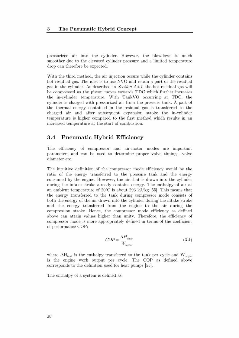
4 Variable Valve Actuation .................................................................... 31 4.1 VVA ........................................................................................... 31 4.2 Camshaft-based VVA Mechanism ............................................... 32 4.2.1 Variable Valve Timing by Camshaft Phasing ..................... 32 4.2.2 Variable Valve Lift by Cam Profile Switching .................... 34
X
4.2.3 Variable Valve Lift by Combining Cam Phasing and Profile Changing ............................................................................. 35
4.2.4 Fully Variable Valve Actuation with Camshaft .................. 37 4.3 Camless VVA Mechanism .......................................................... 37 4.3.1 Electromagnetic Valve Actuation ........................................ 38 4.3.2 Electrohydraulic Valve Actuation ....................................... 39 4.3.3 Electro Pneumatic Valve Actuation .................................... 42
4.4 Valve Strategies Enabled by FVVA ........................................... 45 4.4.1 Negative Valve Overlap ....................................................... 45 4.4.2 Rebreathe Strategy .............................................................. 46 4.4.3 Atkinson/Miller Cycle ......................................................... 48
5 Modeling the Pneumatic Hybrid .......................................................... 49 5.1 Pneumatic Hybrid Engine Modeling in GT-Power ..................... 49 5.2 Pneumatic Hybrid Vehicle Modeling in Simulink/Matlab™ ........ 51
6 Experimental Setup ............................................................................. 56 6.1 Test Engines ............................................................................... 56 6.1.1 Paper I ................................................................................. 56 6.1.2 Paper II and Paper III ......................................................... 58 6.1.3 Paper VI .............................................................................. 59
6.2 Pressure compensated tank valve ............................................... 61 6.2.1 Modifications to the pneumatic spring ................................ 63
6.3 The Engine Control System ....................................................... 64 7 Results ................................................................................................. 66
7.1 Compressor Mode ....................................................................... 66 7.1.1 Efficiency-Optimal Compressor Mode Operation with
Theoretically Calculated Valve Timings .............................. 66 7.1.2 Efficiency-Optimal Compressor Mode Operation with
Optimized Valve Timing ..................................................... 71 7.1.3 The Influence of Valve Head Diameter on Compressor
Mode Performance ............................................................... 73 7.1.4 Compressor Mode Modeling in GT-Power ........................... 78 7.1.5 Parametric Study of Compressor Mode Performance .......... 82 7.1.6 Load Control ....................................................................... 96

XI
7.2 Air-Motor Mode ....................................................................... 100 7.2.1 Initial Testing of Air-Motor Mode ...................................... 100 7.2.2 Optimal Air-Motor Mode Operation .................................. 103 7.2.3 Air-Motor Mode Modeling in GT-Power ............................ 108 7.2.4 Parametric Study of Air-Motor Mode Performance ........... 109
7.3 Drive cycle Simulations ............................................................ 115 7.3.1 Pneumatic Hybrid Performance Maps ................................ 116 7.3.2 Optimal Pressure Tank Volume ......................................... 117 7.3.3 Determining Minimum Tank Pressure ............................... 120 7.3.4 Drive Cycle Simulation Results .......................................... 121
7.4 Regenerative Efficiency ............................................................. 126 8 Summary............................................................................................ 128 9 Discussion .......................................................................................... 130 10 Future Work ...................................................................................... 132 11 References .......................................................................................... 134 12 Summary of Papers ............................................................................ 144
2
Chapter 1
1 Introduction
1.1 Background
The society of today relies to a great extent on different means of transportation. Never before have people travelled to different parts of the world, far away from their own, as today. This massive travelling is a heavy load on our nature. The cars that increase in numbers every day emit toxic emissions on the highways and the airplanes consume huge amounts of fossil fuels. In recent years the awareness of the effect of pollution on the environment and climate has increased. People are more conscious of the situation and are looking for alternative means of transportation with less impact on the environment. The exhaust emission standards are getting more and more stringent and there now exists a discussion about the introduction of a mandatory emissions standard for CO2 [1, 2], a green house gas that contributes to the climate change which is an issue of growing international concern. This demand for lower exhaust emission levels together with increasing fuel prices leads to the demand of combustion engines with better fuel economy, which forces engine developers to find and investigate more efficient alternative engine management.
Today there exist several solutions to achieve lower exhaust emissions and better fuel economy. Some of them are well known while others are still in development. Some examples of such solutions are VVA (Variable Valve Actuation), EGR (Exhaust Gas Recirculation), direct injection, hybridization of vehicles, just to mention a few. In this work the emphasis has been put on vehicle hybridization.
Vehicle hybridization can be done in various ways. The maybe best known example of vehicle hybridization is the electric hybrid. However other hybrids like hydraulic, fuel cell, flywheel and pneumatic hybrids are currently being investigated. The main idea with electric hybridization is to reduce the fuel consumption by taking advantage of the otherwise lost
1.1 Background
3
brake energy. Hybrid operation also allows the combustion engine to operate at its most optimal operating point in terms of load and speed. Today, almost every car manufacturer is working on an electric hybrid prototype and a few already have a product on the market. Electric hybrids offer impressive reductions in fuel consumption. According to Fontaras et al. [3], electric hybrids offer up to 60% lower fuel consumption compared to conventional gasoline fueled vehicles. Folkesson et al. [4] have shown a reduction of over 40% in fuel consumption for a hybrid PEM (Proton Exchange Membrane) fuel cell bus compared to a conventional diesel engine operated bus.
The main disadvantage with electric hybrids is that they require an extra propulsion system and large heavy batteries with a limited life time. This introduces extra manufacturing costs which are compensated by a higher end-product price comparable to the price of high end vehicles. For instance, the purchase cost for a new electric hybrid bus is almost $200 000 higher compared to conventional bus [5]. However, it should be remembered that the high cost will decrease as the sales volume of hybrid vehicles increase.
One way of keeping the extra cost as low as possible and thereby increase customer attractiveness, is the introduction of the pneumatic hybrid. It does not require an expensive extra propulsion source and it works in a way similar to the electric hybrid. During deceleration of the vehicle, the engine is used as a compressor that converts the kinetic energy contained in the moving vehicle into energy in the form of compressed air which is stored in a pressure tank. After a standstill the engine is used as an air-motor that utilizes the pressurized air from the pressure tank in order to accelerate the vehicle. The system supports stop/start functionality, which means that the engine can be shut off during a full stop and thus idle losses can be eliminated [6, 7]. The pneumatic hybrid concept also offers elimination of the “turbo-lag” associated with turbocharged engines by supercharging the engine with pressurized air [8, 9].
Numerous research teams worldwide have demonstrated the potential of the pneumatic hybrid vehicle over the last decade. Tai et al. [7] describes simulations of a pneumatic hybrid with a so called regenerative efficiency of 36% and an improvement by 64% of the fuel economy in city driving. Simulations made by Andersson et al. [10] show simulations where a regenerative efficiency as high as 55% for a dual pressure tank system for heavy duty vehicles was achieved. The fuel consumption reduction for the pneumatic hybrid city bus was in the range of 23%. Trajkovic et al. [11] presented a regenerative efficiency of 48% obtained from engine experiments. In [12], the same research team presented a vehicle model

1 Introduction
4
with an engine model based on experimental data. The model was tested over 10 different drive cycles and the fuel consumption reduction varied between 8 and 58%, depending on drive cycle.
All the presented features of the pneumatic hybrid contribute to lower fuel consumption and in combination with the simplicity of the system, the pneumatic hybrid can be a promising alternative to the traditional vehicles of today and a serious contender to the better known electric hybrid.
1.2 Objective
This thesis is based on a research project started in the beginning of 2006. The research in this work was conducted in close cooperation with Cargine AB, the company developing the pneumatic valve actuating system used in the project. The objective of the project is to study the new pneumatic hybrid concept and its different modes of engine operation. During the first two years of the project fundamental engine experiments were conducted in order to increase the understanding of the operating principle of the different engine modes associated with pneumatic hybridization and the parameters affecting their performance. It was soon realized that an engine model was necessary in order to understand the phenomena that control the pneumatic hybrid. The last couple of years of the project were mainly devoted to modeling of both a pneumatic hybrid engine and a pneumatic hybrid vehicle. The objective was to more thoroughly investigate the different parameters affecting the pneumatic hybrid engine performance and to examine the potential of reduction in fuel consumption for a pneumatic hybrid vehicle.
1.2 Method
For the project summarized in this thesis an approach of both experimental and theoretical nature was chosen. During the first two years of the project, extensive experimental research was conducted with the aim to investigate the feasibility of the pneumatic hybrid concept. The second half of the project was mainly devoted to development of models based on results from engine experimental data. The order of the work conducted in the project, first experiments then modeling, was determined based on the fact that studies done by other researchers until the start of the project were of theoretical nature. Therefore, as a proof of concept it was determined to be more appropriate to start with studies based on
1.4 Thesis Contribution
5
experiments and then use the knowledge gained from these experiments in order to develop more realistic models.
1.4 Thesis Contribution
Prior to the published material described in this thesis, only publications based on results of theoretical nature were available. The experimental work described in this thesis therefore served as a proof of the pneumatic hybrid concept. The in-depth investigation of the different parameters affecting the pneumatic hybrid operation through experiments resulted in more realistic results than what had been shown in earlier studies.
A load control strategy for compressor mode was developed and evaluated. The results proved that the proposed control strategy served its purpose and the compressor mode load was controlled according to the demands with some limitations.
Extensive experimental results from pneumatic hybrid operation are presented. They were used to develop an accurate engine model and through validation against the experimental engine data, more realistic predictions of parameters affecting the pneumatic hybrid operation were realized.
The experience obtained from the experimental studies also lead to a vehicle model with more realistic characteristics than what had previously been shown. Although the model needs further developments, the presences of experimental data leads to more realistic results compared to studies solely based on theoretical knowledge. The model was also used in order to investigate how the pneumatic hybrid performance is affected by different drive cycle characteristics.

6
Chapter 2
2 Vehicle Hybridization
Growing environmental concerns, together with higher fuel prices and more stringent emission legislation, has created a need for cleaner and more efficient alternatives to the propulsion systems of today. Currently vehicles are equipped with engines having a maximum thermal efficiency of 30-40%. The average efficiency is much lower, especially during city driving since it involves frequent starts and stops. One alternative to the propulsion systems of today that has gained momentum over the last decade is the hybridization of vehicles. It has proven significant potential to improve fuel economy and reduce exhaust emissions which, together with tax incentives in some countries and other similar benefits only offered to owners of hybrid vehicles, have contributed to an amazing increase in sales over the last 10-12 years. The currently largest manufacturer of hybrid vehicles, Toyota Motor Corporation (TMC), reports that the cumulative sales of its hybrid vehicles exceeded 2 million units worldwide in August 2009 [13]. TMC estimates that their hybrid vehicles have led to a decrease of about 11 million ton of CO2 emissions.
Figure 1 Toyota Motor Corporation’s cumulative worldwide sales of hybrid vehicles during the period 1998-2009 [13]
The classical definition of a hybrid vehicle is that it is a vehicle that has more than one source of propulsion power. The definition of a hybrid vehicle stated by the European Union in 2007 [14], also includes two
1999 2001 2003 2005 2007 20090
0.3
0.6
0.9
1.2
1.5
1.8
2.1x 10
6
Year
Un
its S
old
2.1 Electric Hybrid Powertrain
7
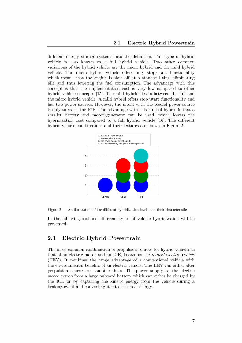
different energy storage systems into the definition. This type of hybrid vehicle is also known as a full hybrid vehicle. Two other common variations of the hybrid vehicle are the micro hybrid and the mild hybrid vehicle. The micro hybrid vehicle offers only stop/start functionality which means that the engine is shut off at a standstill thus eliminating idle and thus lowering the fuel consumption. The advantage with this concept is that the implementation cost is very low compared to other hybrid vehicle concepts [15]. The mild hybrid lies in-between the full and the micro hybrid vehicle. A mild hybrid offers stop/start functionality and has two power sources. However, the intent with the second power source is only to assist the ICE. The advantage with this kind of hybrid is that a smaller battery and motor/generator can be used, which lowers the hybridization cost compared to a full hybrid vehicle [16]. The different hybrid vehicle combinations and their features are shown in Figure 2.
Figure 2 An illustration of the different hybridization levels and their characteristics
In the following sections, different types of vehicle hybridization will be presented.
2.1 Electric Hybrid Powertrain
The most common combination of propulsion sources for hybrid vehicles is that of an electric motor and an ICE, known as the hybrid electric vehicle (HEV). It combines the range advantage of a conventional vehicle with the environmental benefits of an electric vehicle. The HEV can either alter propulsion sources or combine them. The power supply to the electric motor comes from a large onboard battery which can either be charged by the ICE or by capturing the kinetic energy from the vehicle during a braking event and converting it into electrical energy.
Micro Mild Full
1
2
3
4
1. Stop/start Functionality2. Regenerative Braking3. 2nd power source assisting ICE4. Propulsion by only 2nd power source possible

2 Vehicle Hybridization
8
In conventional vehicles the ICE is run at different load points, depending on the current power demand. Switching between different load points will lead to a relatively low average efficiency, since far from all load points offer maximum efficiency. For instance, low load operation suffers from low efficiency due to very high throttling losses. The switching between different load points also has a negative effect on exhaust emissions. For instance, results shown by Samulski et al. [17] indicate a considerable increase in emissions during transient operation.
In a HEV the ICE cooperates with an electric motor, which leads to the possibility of a more optimal use of the ICE. Usually, HEVs use a downsized ICE with reduced size and power. For instance, the Toyota Prius has a 1.5 l engine producing 57 kW (76 hp) of power [18]. The reason is that by downsizing an engine, its power density increases. The engine will be run at a higher average load during a driving cycle which means that the average intake pressure will be higher with lower throttling losses as a result. The reduced peak power of the ICE can be compensated by added power from the electric motor.
Another benefit with the HEV is the possibility of utilizing regenerative braking. Basically, this means that the electric machine can be used as a generator and the energy, otherwise lost during braking, can be stored in the battery for use at a subsequent acceleration of the vehicle.
City driving involves frequent stops and starts of the vehicle. During idling, the ICE consumes fuel without producing useful work thus contributing to higher fuel consumption and unnecessary exhaust emissions. The HEV solves this by shutting off the ICE during a full stop. In this way no fuel will be consumed during idling with no exhaust emissions during this period.
Even though HEVs offers many benefits compared to conventional vehicles, there are some drawbacks making HEVs less appealing in the eyes of the customers. The main disadvantages with electric hybrids are that they require an extra propulsion system and large heavy batteries with a limited life-cycle. This introduces extra manufacturing costs which are compensated by a higher end-product price comparable to the price of high-end vehicles. The limited life expectancy of the batteries also contributes to a higher life-cycle cost of HEVs.
The power sources found in a HEV can be combined in numerous ways. However, the most common drive train configurations are the series and parallel HEV. A series hybrid is a configuration in which only one energy converter can provide propulsion power. The ICE, which is operated in its

2.1 Electric Hybrid Powertrain
9
most optimal regime, drives an electric generator and thus mechanical energy is converted to electrical energy which then is stored in the battery. The propulsion power is provided solely by the electric motor, see Figure 3. The addition of an ICE to the configuration extends the driving range considerably compared to an electric vehicle.
Figure 3 Illustration of a series hybrid drivetrain [19].
In a parallel hybrid, the ICE and the electric motor are connected to the driveshaft through separate clutches. In this configuration the propulsion power can be supplied by the ICE, by the electrical motor, or by a combination of both, see Figure 4. The cooperation between the ICE and the electric machine can be chosen in such a way that the current demand for power can be met. When using only the ICE, the electric machine can function as a generator and charge the battery. The electric machine can also be used during vehicle deceleration to charge the battery. The major advantage of the parallel hybrid compared to the series hybrid is that the possibility of using the ICE as propulsion source leads to fewer energy conversions with less energy conversion losses as a result. One of the drawbacks with this strategy is that during city driving involving long periods of slow driving, the battery can be discharged, forcing the ICE engine to kick in and operate in a regime where it is less efficient.
Figure 4 Illustration of a parallel hybrid drivetrain [19]
2 Vehicle Hybridization
10
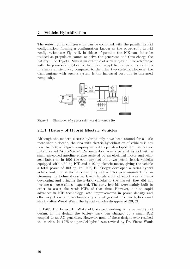
The series hybrid configuration can be combined with the parallel hybrid configuration, forming a configuration known as the power-split hybrid configuration, see Figure 5. In this configuration the ICE can either be utilized as propulsion source or drive the generator and thus charge the battery. The Toyota Prius is an example of such a hybrid. The advantage with the power-split hybrid is that it can adapt to the current conditions in a more efficient way compared to the other two systems. However, the disadvantage with such a system is the increased cost due to increased complexity.
Figure 5 Illustration of a power-split hybrid drivetrain [19]
2.1.1 History of Hybrid Electric Vehicles
Although the modern electric hybrids only have been around for a little more than a decade, the idea with electric hybridization of vehicles is not new. In 1896, a Belgian company named Pieper developed the first electric hybrid called “Auto-Mixte”. Piepers hybrid was a parallel hybrid with a small air-cooled gasoline engine assisted by an electrical motor and lead-acid batteries. In 1901 the company had built two petrol-electric vehicles equipped with a 60 hp ICE and a 40 hp electric motor, giving the vehicle a total power of 100 hp. In 1992, H. Krieger developed a series hybrid vehicle and around the same time, hybrid vehicles were manufactured in Germany by Lohner-Porsche. Even though a lot of effort was put into developing and bringing the hybrid vehicles to the market, they did not become as successful as expected. The early hybrids were mainly built in order to assist the weak ICEs of that time. However, due to rapid advances in ICE technology, with improvements in power density and efficiency, there were no longer any advantages with electric hybrids and shortly after World War I the hybrid vehicles disappeared [20, 21].
In 1967, Dr. Ernest H. Wakefield, started working on a series hybrid design. In his design, the battery pack was charged by a small ICE coupled to an AC generator. However, none of these designs ever reached the market. In 1975 the parallel hybrid was revived by Dr. Victor Wouk
2.1 Electric Hybrid Powertrain
11
and his colleagues. A Mazda rotary engine was coupled with a 15 hp DC machine while the battery for energy storage consisted of eight 12 V automotive batteries. [22]
The great interest in hybrid vehicles today started during the 1990s due to slow advancements in the field of electric vehicles. Toyota was the first company to reach market with the introduction of the Prius in 1997 [21] followed by Honda which two years later introduced the Insight. Today, almost all manufacturers worldwide are putting great effort in the development of electric hybrids indicating a promising future for this type of vehicles.
2.1.2 Fuel Consumption of HEVs
The two first manufacturers to reach the market with their hybrid vehicles were Toyota with the introduction of the Prius in 1997 and Honda which introduced the Insight in 1999. The 2001 Toyota Prius was a full hybrid with an ICE of 76 hp coupled with an electric motor/generator of 67 hp, while the corresponding Honda Insight was a mild hybrid with an ICE of 67 hp assisted by a 13 hp electrical motor. The fuel consumption of the 2001 Honda Insight was 3.9 l/100 km during city driving and 3.5 l/100 km during highway driving. The corresponding figures for the 2001 Toyota Prius are 4.5 and 5.2 l/100 km, respectively [23]. The main reason for the considerable difference in fuel consumption between the two vehicles is that the Insight is a compact car while the Prius is a midsize car with a curb weight about 400 kg higher than the Insight. By comparing the 2001 Toyota Prius to the 2001 Toyota Corolla, which is a conventional vehicle with similar size as the corresponding Toyota Prius, the potential in fuel consumption reduction with hybrid vehicles can be illustrated. The fuel consumption of the 2001 Toyota Corolla was 7.6 l/100 km during city driving and 5.7 l/100 km during highway driving. This corresponds to a fuel consumption reduction of about 38 % and 9%, respectively. Lave et al. presented a similar comparison in [24] where fuel consumption for a Prius and a Corolla during a drive cycle consisting of 55% city driving and 45% highway driving was shown. The fuel consumption was 4.8 and 6.8 l/100 km for the Prius and the Corolla, respectively, which corresponds to a fuel consumption reduction of about 29% for the Prius.
According to EPA [25], the fuel consumption of a 2011 Honda Insight is 5.9 l/100 km during city driving and 5.5 l/100 km during highway driving, while the corresponding fuel consumption for the 2011 Toyota Prius is 4.6 and 4.9 l/100 km, respectively. The reason why the fuel consumption of the 2011 Honda insight has increased compared to the 2001 model is that
2 Vehicle Hybridization
12
the weight of the newer model has increased by about 390 kg and the number of seats has increased from 2 to 5 seats.
In 2002, Chandler et al. [26] presented results achieved for hybrid-electric buses during different driving cycles. The report shows a 20.5% reduction in fuel consumption for a hybrid-electric bus compared to a conventional bus during real city driving, while the corresponding fuel consumption reduction during the Manhattan and New York Bus driving cycles were 32,4% and 39.1% respectively. In 2007, Chiang [27] presented results indicating a fuel consumption reduction of about 29% for a hybrid electric bus during the Manhattan driving cycle.
2.2 Hydraulic Hybrid Powertrain
A hybrid powertrain configuration that is currently subject to extensive investigation by researchers and automotive manufacturers is the hydraulic hybrid vehicle (HHV). The HHV combines an ICE together with a pump/motor and the power supply to the hydraulic motor comes from a hydraulic accumulator. Hydraulic hybrids are characterized by high power density and high storage efficiencies exceeding 95% which makes them suitable for regenerative braking [28].
A considerable advantage with the HHV is that the performance of the hydraulic accumulator, as opposed to the performance of electro chemical batteries, is not degraded by frequent charging/discharging and it is able to accept high rates of energy flow [29]. However, the hydraulic accumulators suffer from a relatively low energy density compared to the electrochemical batteries of the hybrid electric vehicle.
The hydraulic hybrid powertrain basically consists of a hydraulic pump/motor, a hydraulic accumulator and a low pressure hydraulic reservoir. The hydraulic pump/motor is usually of axial piston type. The most common type of hydraulic accumulator is the hydro-pneumatic accumulator which contains compressed air, encapsulated in a bladder, and the hydraulic fluid. The purpose of the reservoir is to collect the low pressure hydraulic fluid that flows through the hydraulic motor after a discharge event and return it the hydraulic pump when needed. [28]
The operating principle of a hybrid vehicle is similar to the electric hybrid. During deceleration of the vehicle, the hydraulic pump captures the brake energy, otherwise lost in the form of heat generated by the friction brakes, and stores it in the hydraulic accumulator by pumping the hydraulic fluid into it and thus increasing the pressure of the compressed

2.2 Hydraulic Hybrid Powertrain
13
air encapsulated by the bladder. This is also known as the pump mode. During the following acceleration of the vehicle, the hydraulic motor utilizes the high-pressure hydraulic fluid in order to generate positive power on the driveshaft. This type of operation is known as motor mode.
As with the electric hybrid, different types of hybrid configurations are possible with the hydraulic hybrid. In the parallel hybrid configuration, the hydraulic pump/motor is connected to the driveshaft via a transmission. In this configuration, the hydraulic pump/motor assists the ICE during acceleration. One advantage with this configuration is that the transfer of power from the ICE to the wheels will remain intact. Another advantage is that the components related to the hydraulic hybrid powertrain can be implemented in a base vehicle without considerable modifications. However, since the ICE is directly connected to the wheels, the engine speed is determined by the vehicle speed and thus ICE operation in low efficiency regimes cannot be avoided. [30]
In the series hybrid configuration, the ICE is no longer mechanically connected to the wheels. The ICE, which is operated in the most optimal regime, is connected to a hydraulic pump and thus mechanical energy can be converted to pressure energy which then is stored in the hydraulic accumulator. When the accumulator reaches its upper limit, the engine is shut off and the vehicle is then propelled by energy supplied by the accumulator. The propulsion power is provided solely by the hydraulic motor. This configuration also offers the possibility to place hydraulic pumps/motors at each wheel which enables individual wheel torque control. The disadvantage with this configuration is that the power transmission becomes less efficient with increased number of energy conversions. [30]
2.2.1 Fuel Consumption of HHVs
In resemblance to electric hybridization, hydraulic hybridization offers impressive reduction in fuel consumption. Alson et al. [31] investigates the fuel consumption reduction for a SUV and a midsize car with hydraulic hybrid powertrain compared to their conventional counterparts. The conventional SUV shows a fuel consumption of 13.7 l/100 km, while the corresponding hydraulic hybrid shows a fuel consumption of 10.2 l/100 km which results in a reduction of about 25%. The fuel consumption for the conventional midsize car was 8.1 l/100 km, while the fuel consumption for the hydraulic hybrid counterpart was 5.4 l/100 km. This results in a fuel reduction of about 33%.

2 Vehicle Hybridization
14
In [28] Filipi et al. Presented results for a hydraulic hybrid Hummer with a 4.5 L V6 engine over the EPA Urban Schedule. The fuel consumption reduction of the hydraulic hybrid Hummer compared to its conventional counterpart was about 42%. In 2009, Johri et al. [32] compared a hydraulic hybrid to the first generation of Honda’s electric hybrid Insight. The fuel consumption reduction over an urban driving cycle for the hydraulic hybrid compared to the Honda Insight reached an impressive 46% while the corresponding fuel consumption reduction over a highway driving cycle was about 16%. The fact that the hydraulic hybrid was compared to an already fuel efficient vehicle and that the fuel consumption reached as high as 46% percent demonstrates the extreme potential with hydraulic hybridization.
2.3 Fuel Cell Hybrid Powertrain
Fuel cells for use in automotive applications have been under intensive research over the last few decades. By adding a fuel cell to an electric driveline, a fuel cell hybrid vehicle (FCHV) is created. Usually, a fuel cell is fitted to a series hybrid electric driveline for which the energy is supplied by the batteries and the fuel cell. The fuel cell most commonly uses hydrogen as fuel and the power produced by it is stored in an electric battery or directly used by an electric motor. The advantage of using fuel cells in hybrid configuration is that at high loads, power can be supplied by the battery and therefore the size, weight and volume of the fuel cell can be kept at a minimum. In an optimized system configuration, the fuel cell can be allowed to operate at constant load and thus the fuel cell efficiency can be maximized [33].
The main parts of a fuel cell are an anode, an electrolyte and a cathode. The fuel is supplied in a pressurized state to the anode at which it comes into contact with the catalytic layer of the anode and dissociates into electrons and protons. The protons continue their journey through an electrolytic substance towards the cathode while the electrons are blocked from entering it. Instead the electrons are redirected towards the cathode via an external circuit in which an electric current is generated. Pressurized oxygen is provided to the cathode. When the oxygen comes into contact with its catalytic layer, it reacts with the protons and the redirected electrons and water and heat is produced. [34]
There are a couple of different fuel cell types. The most common type researched for automotive applications is the proton exchange membrane (PEM) fuel cell. It uses a solid polymer membrane as electrolyte and the working temperature is 60-100°C. The PEM fuel cell is fueled with pure

2.3 Fuel Cell Hybrid Powertrain
15
H2 and O2 or air as oxidant. An advantage with the PEM is its high power density which results in a small size of the fuel cell. [21]
Another type of fuel cell used in automotive applications is the solid oxide fuel cell (SOFC). In conformity with PEM fuel cells, the SOFC uses a solid electrolyte, in this case a solid ceramic membrane. The working temperature of the SOFC exceeds 1000°C which has to be considered a safety issue in automotive applications. Also, the high temperature implies that the fuel cell has to be heated which results in increased fuel consumption. Another disadvantage with the SOFC is its quite brittle ceramic electrolyte which might pose a problem in a vehicle subjected to stong vibrations. [21]
The first company to demonstrate a FCHV was Honda with the unveiling of their prototype Honda FCX at the Tokyo Motor Show in 1999. The FCX was equipped with an electric motor with a maximum power output of 80 kW together with a PEM fuel cell with maximum power output of 86 kW. The FCX had a top speed of 150 km/h and offered a driving range of up to 430 km [35]. In 2007, Honda introduced the FCX Clarity which was an improved version of Honda FCX. The PEM fuel cell power output was increased to 100 kW and the driving range was increased by 30% [36]. Also Toyota has been working on FCHV the past decade. In 1999, Toyota unveiled their first fuel cell hybrid, the FCHV-1. The FCHV-1 utilized an electric motor together with a PEM fuel cell, each with a maximum power output of 90 kW. The maximum speed was 155 km/h and the driving range was about 330 km. In 2008, Toyota introduced a more advanced version of the FCHV-1, namely the FCHV-adv. The power output of the electric motor and the fuel cell of the FCHV-adv is the same as for its predecessor. However, the driving range has been increased to 830 km. The more than doubled driving range compared to its predecessor is a result of higher fuel efficiency and an increased hydrogen storage pressure [37].
In [38] Folkesson et al. presented results for a Scania hybrid PEM fuel cell concept bus. The bus was equipped with a 50 kW fuel cell and two 50 kW wheel hub motors. The fuel cell efficiency reached 41% and the fuel consumption reduction was between 42 and 48% compared to a standard Scania bus. Ahluwalia et al. [39] reported a fuel consumption reduction between 54 and 69%, depending on drive cycle, for a FCHV compared to a corresponding ICE powered vehicle.
2 Vehicle Hybridization
16
2.4 Flywheel Hybrid Vehicle
With the introduction of kinetic energy recovery systems (KERS) in Formula 1 for 2009, a system developed by Flybrid Systems LLP gained considerable attention. The system uses a flywheel based mechanical hybrid driveline in which the kinetic energy of the vehicle can be transferred to a flywheel during deceleration and brought back to the drive-wheels during subsequent acceleration of the vehicle. This type of hybrid configuration is referred to as flywheel hybrid vehicle (FHV). The basic idea with FHVs is to use a flywheel as a mechanical battery that can absorb, store and release energy. The flywheel is connected to the driveline by a continuously variable transmission (CVT). During a braking event, the kinetic energy of the vehicle is transferred to the flywheel which causes the flywheel to increase its rotational speed. During the following standstill, the flywheel keeps rotating at a high speed since the flywheel is encapsulated with high vacuum. During the subsequent acceleration event, the kinetic energy of the flywheel is transferred back to the vehicle which causes the flywheel to decrease its rotational speed. With the CVT the rate of energy transferred to/from the flywheel can be continuously controlled. [40, 41]
In [40], Cross et al. demonstrates a fuel consumption reduction of up to 21.9% for light-duty vehicles utilizing the flywheel hybrid driveline, while Brockbank et al. [41] showed a fuel consumption reduction of about 34% for a flywheel hybrid city bus. Both studies show a regenerative efficiency above 70%.
2.5 Pneumatic Hybrid Powertrain
As stated earlier, the main drawbacks with electric hybrids are that they require an additional propulsion system and large, heavy batteries. All of this costs the manufacturers a lot of money, which is compensated by a higher end-product price. One way of keeping the extra cost as low as possible and thereby increase customer attractiveness, is the introduction of the pneumatic hybrid vehicle (PHV). In contrast to the other hybrid configurations, the pneumatic hybrid is a relatively simple solution utilizing only an ICE as propulsion source. Instead of expensive batteries with a limited life-cycle, the pneumatic hybrid utilizes a relatively cheap pressure tank to store energy. In order to run the engine as a pneumatic hybrid, a pressure tank has to be connected to the cylinder head in some way. Tai et al. [42] describe an intake air switching system in which one inlet valve per cylinder is fed by either fresh intake air or compressed air from the pressure tank. Andersson et al. [43] describes a dual valve system
2.5 Pneumatic Hybrid Powertrain
17
where one of the intake ports has two valves, one of which is connected to the air tank. A third solution would be to add an extra port to the cylinder head, which would be connected to the air tank. Guzzella et al. [44] presents a solution where the pneumatic hybrid engine is equipped with a charging valve in addition to the conventional intake and exhaust valves. Since these three solutions demand significant modifications to a standard engine a simpler solution, where one of the existing inlet valves is converted to a tank valve, has been chosen and used in present thesis. The drawback with this solution is that there will be a significant reduction in peak power, and reduced ability to generate and control swirl for good combustion. Another prerequisite for pneumatic hybridization is a fully variable valve actuation system to control the valves and thereby control the pressurized air flow to and from the tank.
Pneumatic hybrid operation introduces new operating modes in addition to conventional ICE operation. During deceleration of the vehicle, the engine is used as a compressor that converts the kinetic energy of the vehicle into potential energy in the form of compressed air which is stored in a pressure tank. This kind of operation is referred to as the compressor mode (CM). After a standstill, the engine is used as an air-motor that utilizes the pressurized air from the tank in order to accelerate the vehicle. This type of engine operation is known as the air-motor mode (AM). A third possible mode of operation is the air-power assist mode (APAM). During APAM the stored compressed air is used for supercharging the engine when there is a demand for higher torque, for instance during the turbo-lag period. During periods when no energy is required from the engine, like idling and when the gas pedal is released, the ICE can be completely shut off. This means that during such periods there will be no fuel consumption and thus no exhaust emissions.
The fuel saving potential of the pneumatic hybrid has been investigated by numerous research teams over the past decade. In 1999, Schechter [45] demonstrated a fuel consumption reduction of 50% for a vehicle weighing about 1300 kg equipped with a 2-liter gasoline engine. Even though the simulation model was of extremely basic nature, the results served as an indicator of the potential with pneumatic hybridization and triggered other research teams to further develop the concept. In 2003 Thai et al. [42] presented a more advanced model of a pneumatic hybrid vehicle. The results indicated a fuel consumption reduction of about 39% for a vehicle similar to the one used by Schechter [45]. Andersson et al [43], presented a pneumatic hybrid city bus utilizing two pressure tanks. The function of the second pressure tank was to substitute the atmosphere as a supplier of low pressure air. By maintaining a pressure level above ambient pressure, a very high torque during compressor mode could be achieved. The fuel
2 Vehicle Hybridization
18
consumption reduction for the pneumatic hybrid city bus was in the range of 23%. Trajkovic et al. [46] presented experimental results for a single-cylinder Scania heavy-duty diesel engine. A regenerative efficiency of up to 32% was demonstrated. In 2008, the same research team showed in [47] a regenerative efficiency of 48% achieved with optimized tank valve geometry and valve timings. In [48] Trajkovic et al. presented a vehicle model with an engine model based on experimental data. The model was tested over 10 different drive cycles and the fuel consumption reduction varied between 8 and 59%, depending on drive cycle.
2.5.1 History of Pneumatic Hybrid Vehicles
As with HEVs, the idea of hybrid pneumatic vehicles is far from new. In 1909, J.K. Broderick filed for a patent titled “Combined internal combustion and compressed air engine” [49]. He wrote in his application that his idea was to use compressed air together with an engine used for propelling a vehicle. The purpose of the compressed air is to assist the engine in starting when under heavy load, or when going uphill. The proposed configuration is also capable of generating compressed air which is stored in a tank. The compressed air can then be used for the purpose of illuminating the vehicle, for starting the ICE or to actuate the vehicle brakes. The compressed air is generated by two cylinders in a four-cylinder engine, and the remaining two cylinders operate in the usual manner. This can only be done while driving downhill or if the vehicle is at rest. He also mentions that the compressed air alone can be used for driving the vehicle.
In 1950, W.G Ochel et al. [50] came up with the idea of using a multicylinder engine to generate compressed air. The inventors stated that at that time, compressed air was normally generated by a compressor driven by an ICE, which lead to the requirement of increased space together with higher investment and maintenance cost. Their proposal was to use a multi-cylinder engine, where a number of cylinders operate in a normal manner while the remaining cylinders compress air which then is stored in a pressure tank. This idea reminds a lot of the one patented by Broderick and the only difference seems to be that Broderick’s invention was intended for use in a vehicle, while Ochel’s invention was intended for stationary use where the compressed air would be used for actuating drill hammers, spray guns for painting, etc.
R. Brown describes, in a patent filed in 1972, an air engine powered by compressed air as an environmentally friendly alternative to the ICE which emits toxic exhaust gases [51]. In Brown’s invention the compressed air is generated by a compressor driven by an electric motor.

2.5 Pneumatic Hybrid Powertrain
19
In 1974, T. Ueno, filed for a patent which bore a great resemblance with Broderick’s invention [52]. It involved compression of air by dedicated engine cylinders and utilization of compressed air in order to propel the vehicle. The main difference was that Ueno’s invention was also capable of regenerative braking, which was not possible with Broderick’s design.
With David Moyers invention, patented in 1996 [53], the definition of the pneumatic hybrid as it is known today was complete. His idea was to add the supercharge mode, which meant that the intake pressure was raised beyond ambient pressure by the induction of compressed air stored in a pressure tank.

20
Chapter 3
3 The Pneumatic Hybrid Concept
The pneumatic hybrid vehicle (PHV) concept is a low-cost alternative to the more established electric hybrid. The PHV concept comprises no additional propulsion source and a pressure tank as an energy storage device. The main idea with the pneumatic hybrid is to use the ICE in order to compress atmospheric air and store it in a pressure tank when decelerating the vehicle. The stored compressed air can then be used either to accelerate the vehicle or to supercharge the engine in order to achieve higher loads when needed.
The pneumatic hybrid engine configuration chosen for the different studies presented in the thesis comprises a dedicated tank valve or charging valve that controls the flow of compressed air into or out from a pressure tank connected to the tank valve port on the cylinder head. All valves are controlled by a fully variable valve actuating system.
Before explaining the operation of the different pneumatic hybrid engine modes of operation, some important performance parameters need to be explained. By plotting the cylinder pressure against corresponding cylinder volume, a PV-diagram is generated. The area enclosed by the PV-diagram is the indicated work (Wi) done by the gas on the piston:
iW pdV (3.1)
The load of the engine can be expressed as the indicated mean effective pressure (IMEP). IMEP is a quantity related to the indicated work output of the engine independent of engine displacement which makes comparison between different engines of different sizes possible. IMEP is defined as the ratio of indicated work to the engine displacement:
i
d
WIMEPV
(3.2)

3.1 Compressor Mode
21
In the following sub-sections the most important pneumatic hybrid engine modes of operation will be thoroughly discussed. In addition, a sub-section dealing with PHV efficiency and a sub-section explaining why two-stroke operation was chosen for the present study will be presented.
3.1 Compressor Mode
In compressor mode, the engine is utilized as a 2-stroke compressor in order to decelerate the vehicle. The kinetic energy of the moving vehicle is converted to potential energy in the form of compressed air. The ideal operating principle of the compressor mode can be explained with references to Figure 6. The numbers in brackets refer to the numbers in the PV-diagram displayed in Figure 6(b).
1 – 2: Intake stroke. During compressor mode operation the inlet valve opens a number of crank angle degrees (CAD) after top dead centre (ATDC) and fresh air is brought to the cylinder (1). At the end of the intake stroke, as the piston reaches bottom dead centre (BDC), the inlet valve closes (2).
2 – 3: Compression stroke. The moving piston starts to compress the air trapped in the cylinder as it ascends away from BDC. The compression stroke ends at the moment the tank valve opens.
3 – 4: Charging period. The charging period is the period during which the compressed air is transferred from the cylinder into the pressure tank. It starts when the tank valve opening (TankVO) occurs. The opening is set to occur somewhere between BDC and top dead centre (TDC) (3), depending on how much braking torque is needed. For instance, a very early TankVO means that there will be a blowdown of pressurized air into the cylinder, and the piston has to work against a much higher pressure, thus a higher braking torque is achieved. The charging period proceeds as long as the tank valve is open. The tank valve closing (TankVO) occurs shortly after TDC (4). At this point the cylinder contains compressed air at the same pressure level as the air in the tank.
4 – 1: Expansion stroke. As the piston descends away from TDC, the compressed air trapped in the cylinder expands and the intake valve opening (IVO) occurs when ambient pressure is reached in the cylinder (1). A too early IVO means that there will be a blowdown of the compressed air trapped in the cylinder into the intake manifold, thus useful energy is wasted. A too late IVO, on

3 The Pneumatic Hybrid Concept
22
the other hand, leads to over-expansion of the air trapped in the cylinder which results in the generation of vacuum. Since this is an energy consuming process, the net result will be an increase in negative load.
(a) (b) Figure 6 (a) Illustration of compressor mode operation, I) Intake of fresh air, II)
Compression of air and pressure tank charging; (b) Cylinder pressure during ideal compressor mode operation presented as a function of cylinder volume in a PV-diagram.
By operating the compressor mode according to the description given above maximum compressor mode efficiency will be achieved. However, during real driving, the braking power generated during compressor mode operation, will vary according to the current driving conditions. This means that ideal operation cannot be maintained at all time and thus the compressor mode efficiency will decrease.
3.1.1 Load Control of Compressor Mode
An important aspect of the pneumatic hybrid concept is its ability to control the amount of braking torque generated at a specific time during compressor mode operation. As stated above, the load demand during compressor mode operation will be far from optimal in terms of efficiency. In Figure 7, the compressor mode torque distribution as a function of tank pressure during a standard driving cycle, in this case the Braunschweig cycle, is illustrated. The torque data is supplemented by data from optimal compressor mode operation visualized as a dashed line in present figure. It can clearly be seen that most of the operating points will deviate considerably from optimal operation. This leads to the conclusion that running the engine only in optimal operating points is not realistic. The

3.1 Compressor Mode
23
Figure 7 Torque distribution during compressor mode operation as a function of tank pressure during the Braunschweig driving cycle.
load will depend on the driving conditions and the tank pressure. Therefore, the need for a more advanced load control is evident. Below, the control strategy developed in the present study will be discussed.
The development of the load controller was done in two steps. At first, a feedforward controller was tested. The feedforward controller contains valve timing data acquired from steady-state experiments at different loads and tank pressures. The results are displayed in Figure 8 in the form of a TankVO map. From the figure it can be noticed that the compressor mode operation is limited on two fronts. The occurrence of the lower limit, can be explained by inadequate amount of tank pressure which prevents the compressor mode operation to achieve higher loads. For instance, at a tank pressure of 5 bar the maximum achievable load is almost 4 bar. The maximum load is achieved when the tank valve opens at BDC. At this point, maximum charging capacity of the cylinder has been reached and the cylinder cannot be filled with any additional amount of pressurized air, and hence a further increase in load at this tank pressure cannot be achieved. The occurrence of the upper limit shown in Figure 8 can be explained by improper valve actuator function. A low load demand at a high tank pressure will lead to a TankVO close to TDC and since tank valve closing (TankVC) occurs at TDC or shortly after a too short tank valve duration can be expected. With extremely short tank valve durations, the stability of the valve actuators deteriorates considerably. In order to ensure proper valve actuator functionality at all times both limits have been implemented as constraints in the control program.
The feedforward controller takes the measured load and tank pressure from the previous engine cycle as inputs and with the help of the map presented in Figure 8, the controller outputs proper steady-state valve timings at current tank pressure and load. In Figure 9, the process

3 The Pneumatic Hybrid Concept
24
Figure 8 Illustration of the feedforward load controller map of the TankVO as a function of both IMEP and tank pressure. TankVO is expressed in CAD ATDC.
response to a set point change in IMEP when using the previously described controller can be seen. The process variable deviates from the set point both before and after the load step, which indicates the disadvantage with using a pure feedforward controller. The reason for this behavior is that the conditions in- and outside the engine might not be the same as at the time the valve timing maps used with the feedforward controller were generated. Factors like intake air temperature, engine oil and coolant temperatures and valve actuator nonlinearities contribute considerably to this type of behavior.
Figure 9 Process response to a set-point change in IMEP when using a feedforward load controller during compressor mode operation at a steady-state tank pressure of 5 bar.
In order to avoid the unwanted behavior described above, a closed-loop controller has to be added to the control system. In the project described in the thesis, the feedforward was combined with an ordinary PID controller. The task of the PID controller is to eliminate any steady-state
IMEP [bar]
Ta
nk
Pre
ssu
re [b
ar]
-60-80 -100
-120
-140
2 4 6 84
6
8
10
12
Lower Limit
Upper Limit
0 50 100 150 200 250 3002.4
2.5
2.6
2.7
2.8
2.9
3
3.1
3.2
3.3
IME
P [b
ar]
Engine Cycles [-]
MeasuredSetpoint
3.2 Air-Motor Mode
25
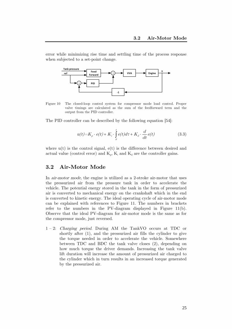
error while minimizing rise time and settling time of the process response when subjected to a set-point change.
Figure 10 The closed-loop control system for compressor mode load control. Proper valve timings are calculated as the sum of the feedforward term and the output from the PID controller.
The PID controller can be described by the following equation [54]:
t
p i d0
du(t)=K e(t) K e(t)dτ K e(t)dt
(3.3)
where u(t) is the control signal, e(t) is the difference between desired and actual value (control error) and Kp, Ki and Kd are the controller gains.
3.2 Air-Motor Mode
In air-motor mode, the engine is utilized as a 2-stroke air-motor that uses the pressurized air from the pressure tank in order to accelerate the vehicle. The potential energy stored in the tank in the form of pressurized air is converted to mechanical energy on the crankshaft which in the end is converted to kinetic energy. The ideal operating cycle of air-motor mode can be explained with references to Figure 11. The numbers in brackets refer to the numbers in the PV-diagram displayed in Figure 11(b). Observe that the ideal PV-diagram for air-motor mode is the same as for the compressor mode, just reversed.
1 – 2: Charging period. During AM the TankVO occurs at TDC or shortly after (1), and the pressurized air fills the cylinder to give the torque needed in order to accelerate the vehicle. Somewhere between TDC and BDC the tank valve closes (2), depending on how much torque the driver demands. Increasing the tank valve lift duration will increase the amount of pressurized air charged to the cylinder which in turn results in an increased torque generated by the pressurized air.
VVA EngineFeed
Forward
PID
ref
‐1
yTank pressure

3 The Pneumatic Hybrid Concept
26
(a) (b) Figure 11 (a) Illustration of air-motor mode operation, I) Charging of the cylinder with
pressurized air, II) Air venting; (b) Cylinder pressure during ideal air-motor mode operation presented as a function of cylinder volume in a PV-diagram.
2 – 3: Expansion stroke. As the piston descends away from TDC, the pressurized air contained in the cylinder is expanded. The expansion stroke ends at BDC (3) at which point the inlet valve opens.
3 – 4: Exhaust stroke. As the piston ascends away from BDC the air contained in the cylinder is expelled to the inlet manifold. Closing of the inlet valve occurs somewhere between BDC and TDC (4), and the timing is selected in such a way that when the piston reaches TDC, the air trapped in the cylinder is compressed to the same level as the tank pressure. It can be noticed that this method of altering the length of the compression stroke is very similar to the late Miller cycle which will be described in Section 4.4.3. If the inlet valve closes too late, the pressure in the cylinder at TDC will be below the tank pressure level, and as soon as the tank valve opens a blowdown of pressurized air into the cylinder will occur. In Section 7.2.4 it will be shown that this leads to a decrease in air-motor mode efficiency.
Above, the ideal operating principle of the air-motor mode has been presented. However, during real driving the demanded load during air-motor mode will be determined by the current driving conditions which consequently mean that the air-motor mode operation will deviate from the ideal case substantially. A high load demand means that the charging period will be extended. This might lead to a situation where the pressure at the end of the expansion stroke is above atmospheric pressure resulting in a blowdown of pressurized air into the intake manifold at the time of

3.2 Air-Motor Mode
27
IVO. This is a waste of useful energy and such operation of AM should be avoided as much as possible.
3.3 Air-Power Assist Mode or Supercharge Mode
An interesting feature introduced with pneumatic hybridization is the ability to supercharge the engine with the purpose of increasing load during fired engine cycles. This type of operation is referred to as the air-power assist mode or supercharge mode. This mode can be used in order to reduce the turbo-lag which can be experienced in vehicles equipped with a large turbocharger. The turbo-lag is the time it takes for the turbine to reach necessary speed from the moment the driver has pressed the gas pedal. A large turbocharger implies a high inertia of the rotating parts which consequently leads to a large turbo-lag period. By injecting pressurized air into the cylinder, the amount of air mass in the cylinder can be increased which enables a larger mass of fuel to be burned during combustion and thus a higher load can be realized. In theory the torque can be increased instantly during supercharge mode. However, due to time delays in the VVA and control system, a torque increase within a couple of engine cycles can be expected.
Supercharging of the engine with pressurized air can be done in a couple of ways:
Injection of pressurized air at BDC
Injection of pressurized air during the compression stroke
Injection of pressurized air at TDC in combination with NVO.
The first method is achieved with TankVO at BDC before the compression stroke begins. The cylinder is filled with the required amount of pressurized air with regards to the demanded load. After TankVC the air contained in the cylinder is compressed and eventually combustion is initiated. The main disadvantage with this method is that, since the pressure in the cylinder at TankVO is at atmospheric level, there will be a blowdown of pressurized air from the tank into the cylinder. This blowdown will lead to an expansion of the pressurized air with a decrease in in-cylinder temperature as a result which might aggravate the initiation of the combustion and lead to misfire.
The second method avoids the problem identified in previous method by retarding the TankVO to the point in the compression stroke where the pressure in the cylinder reaches a level slightly below the pressure level in the pressure tank. The pressure difference leads to a charging of
3 The Pneumatic Hybrid Concept
28
pressurized air into the cylinder. However, the blowdown is much smoother due to the elevated cylinder pressure and a limited temperature drop can therefore be expected.
With the third method, the air injection occurs while the cylinder contains hot residual gas. The idea is to use NVO and retain a part of the residual gas in the cylinder. As described in Section 4.4.1, the hot residual gas will be compressed as the piston moves towards TDC which further increases the in-cylinder temperature. With TankVO occurring at TDC, the cylinder is charged with pressurized air from the pressure tank. A part of the thermal energy contained in the residual gas is transferred to the charged air and after subsequent expansion stroke the in-cylinder temperature is higher compared to the first method which results in an increased temperature at the start of combustion.
3.4 Pneumatic Hybrid Efficiency
The efficiency of compressor and air-motor modes are important parameters and can be used to determine proper valve timings, valve diameter etc.
The intuitive definition of the compressor mode efficiency would be the ratio of the energy transferred to the pressure tank and the energy consumed by the engine. However, the air that is drawn into the cylinder during the intake stroke already contains energy. The enthalpy of air at an ambient temperature of 20°C is about 293 kJ/kg [55]. This means that the energy transferred to the tank during compressor mode consists of both the energy of the air drawn into the cylinder during the intake stroke and the energy transferred from the engine to the air during the compression stroke. Hence, the compressor mode efficiency as defined above can attain values higher than unity. Therefore, the efficiency of compressor mode is more appropriately defined in terms of the coefficient of performance COP:
k
engine
HCOPW
tan (3.4)
where ΔHtank is the enthalpy transferred to the tank per cycle and Wengine
is the engine work output per cycle. The COP as defined above corresponds to the definition used for heat pumps [55].
The enthalpy of a system is defined as:

3.5 2-stroke vs. 4-stroke
29
H U pV (3.5)
where U is the internal energy of the system, p and V are the pressure and volume, respectively, of the system.
The internal energy of a system can be expressed as:
vU=mC T (3.6)
By inserting (3.6) in (3.5) followed by differentiation the change in enthalpy can be expressed as:
v vdH=mC dT C Tdm Vdp pdV = 0
(3.7)
If equation (3.7) is applied to the pressure tank, the last term should be deleted since the volume of the tank is constant.
The air-motor mode efficiency can be defined as the ratio between the work produced by the engine and the energy transferred from the pressure tank to the cylinder:
engineAM
tank
Wη =
ΔH (3.8)
Another important parameter is the regenerative efficiency which serves as an indicator of how much of the energy absorbed during braking that can be regenerated into useful work. It is defined as the ratio between the work generated by the engine during air-motor mode operation and the work absorbed by the engine during compressor mode operation:
AMregen
CM
WW
(3.9)
3.5 2-stroke vs. 4-stroke
In previous sub-sections, the compressor mode and the air-motor mode were both described as two-stroke modes, which means that it takes two strokes to complete a cycle. However, a few researchers have presented corresponding modes operated in four-stroke mode [56,57,58]. The reason is that, by operating the pneumatic hybrid engine in four-stroke mode a less complex, low cost alternative can be realized. Dönitz et al. [57]

3 The Pneumatic Hybrid Concept
30
presented a solution where the intake and exhaust valves remain camshaft driven and only the tank valve is fully variable. During the pneumatic hybrid engine modes, the engine is operated in four-stroke mode. Lee et al. [58] presented a solution completely without VVA. During operation of the pneumatic hybrid modes, a set of throttles placed in the intake manifold directed the flow from or to the tank. By operating the pneumatic hybrid in these ways, the dependence of fully variable valve actuation can be avoided and thus keeping the manufacturing cost to a minimum. However, without a VVA system the operation of the different modes becomes very restricted. Operating in 4-stroke mode, the power output is halved compared to 2-stroke mode (1 power stroke versus 2 power strokes per crankshaft revolution). With a VVA, the pneumatic hybrid engine modes of operation can be operated in n-stroke mode where n is any multiple of 2, and thus a more precise control of the power output can be achieved. For instance, if a very low load is demanded during air-motor mode operation, it might be more efficient in terms of pressurized air usage to operate the engine in 6-stroke mode at a higher load compared to operation in 2-stroke mode at a much lower load. However, no studies have so far been done that can attest the validity of this statement.
In this thesis, it was quite natural to operate the different modes in 2-stroke mode due to the presence of a fully variable valve actuating system.

31
Chapter 4
4 Variable Valve Actuation
As was shown in Sections 3.1 and 3.1, the valve timings are probably the most important parameters affecting the performance of the various pneumatic hybrid engine modes of operation. Some research teams have presented solutions where the valves are actuated with a conventional camshaft. However, this limits the different modes of operation considerably. Therefore, a variable valve actuating system is more or less a prerequisite for satisfying pneumatic hybrid engine operation. The present chapter is mainly devoted to VVA systems and information on both camshaft-based and camless VVA systems will be given. Since there are many ways in which this can be achieved, only the most common systems will be briefly described. Also some of the most commons valve strategies enabled by VVA will be presented.
4.1 VVA
Since the beginning of the ICE history, almost all engines have had some sort of valve design for the gas exchange process. The purpose of the gas exchange process is to remove the burnt gases from the combustion chamber and admit a fresh charge of air (direct injected ICE) or air and fuel (port injected ICE) for the next cycle.
The disadvantage with conventional valve actuation in combustion engines is that once the camshaft has been configured and produced, its characteristics can never be changed. Since optimal timing and lift settings are different at high and low engine speeds, the fixed valve timing in engines using conventional valve actuation has to be a compromise between these two. For instance, a mid-size car with engine speeds hardly exceeding 3000 rpm uses a small valve overlap. The valve overlap means that both the exhaust and the inlet valve s are open at the same time and its purpose is to promote induction of fresh charge into the cylinder by using the vacuum created by the outgoing exhaust gases. A small overlap gives the engine a smooth idle and good low speed torque. Race cars mainly with engines mainly operating at high engine speeds, on the other

4 Variable Valve Actuation
32
hand, use large valve overlaps. A large valve overlaps allows good engine breathing at high engine speeds but causes a rough idle and poor performance at low engine speeds. It is evident that in order to design an engine with good performance at both low and high engine speeds, the valve timings cannot be fixed and thus VVA is needed. Variable valve actuation is a generalized term used to describe the altering of the valve lift event by means of variable valve timing, lift and duration.
4.2 Camshaft-based VVA Mechanism
The most widely used mechanism for VVA utilizes a specially designed camshaft as main component. In this type of VVA systems the camshaft has some extra features for changing the valve timing or valve lift, or a combination of both. Some of the various systems will be described below.
4.2.1 Variable Valve Timing by Camshaft Phasing
In a cam phasing system, the camshaft can be rotated with respect to the crankshaft and thereby the valve timing can be changed while the valve duration and lift stays unaffected. Simpler systems only offer shifting between two fixed positions while more complex systems feature continuously variable valve timings within a defined crank angle range.
Alfa Romeo was the first manufacturer to use a variable valve timing system in production cars. The patent for the system was filed 1979 in the USA [59] and models stating from 1984 used a phasing of the intake cam relative to the crankshaft [60]. The system is illustrated in Figure 12. What characterizes this system is that the intake valve duration remains constant while inlet valve opening and closing are moved equally, see Figure 13. At low loads and low engine speeds it is beneficial to retard the
Figure 12 Alfa Romeo cam phasing mechanism using helical and straight splines [61].

4.2 Camshaft-based VVA Mechanism
33
Figure 13 Illustration of inlet valve cam phasing
intake valve event, since the reduced valve overlap results in improved combustion (no blow back of exhaust gases to the intake side) and a delayed inlet valve closing reduces throttling losses. In low to medium speed range, the intake valve event is advanced and thereby the valve overlap is increased. The earlier inlet valve closing prevents the already inducted air from being expelled, thus increasing the power output. At high engine speeds it is favourable with late inlet valve closing in order to take advantage of the intake system ram effect (pressure wave propagation) and since the reduced valve overlap contributes to a lower residual gas fraction, the mass of the inducted air/fuel mixture is maximized with a higher engine power output as a result. Figure 14 shows the cam phasing strategy throughout the whole engine speed range for a Mercedes-Benz 500 SL.
Figure 14 Variable valve timing map for a Mercedes-Benz 500 SL [62]
Toyota introduced a continuously controlled cam phasing system in 1996. It is known as the VVT-i system and it offers continuously variable intake

4 Variable Valve Actuation
34
cam phasing by up to 60 crank angle degrees. The VVT-i system showed improvements in fuel economy by 6%, compared to a similar engine using a conventional camshaft [63].
4.2.2 Variable Valve Lift by Cam Profile Switching
A drawback with cam phasing is that the valve event duration and valve lift height are unaffected. Unaffected valve duration means that if inlet valve opening is retarded, then inlet valve closing is also retarded by the same amount, which in some situations leads to reduced amount of charge entering the cylinder. Thus could be avoided with a system that allows altering of the valve event duration. In this way, inlet valve closing can be adjusted for maximum volumetric efficiency at higher engine speeds and larger valve overlap.
The valve lift is also an important factor affecting engine performance. At low engine speeds, a lower valve lift is preferable, since it promotes more turbulence. At high engine speeds the vale lift height is set to a maximum in order to achieve efficient breathing. Figure 15 illustrates typical valve timing and valve lift height for a two-step cam profile switching system.
Figure 15 Illustration of two-step cam profile switching
Honda has developed a system called VTEC (Variable valve Timing and lift Electronic Control) which allows switching between two different cam profiles [64]. The engine has two low-speed cam lobes and one high-speed cam lobe, see Figure 16(a). As the engine moves into different speed ranges, the engine controller can activate different lobes on the camshaft and change the cam timing. In this way, the engine gets the best features of low-speed and high-speed camshafts in the same engine.
Mitsubishi has developed a system similar to Honda’s VTEC which is known as MIVEC (Mitsubishi Innovative Valve timing and lift Electronic
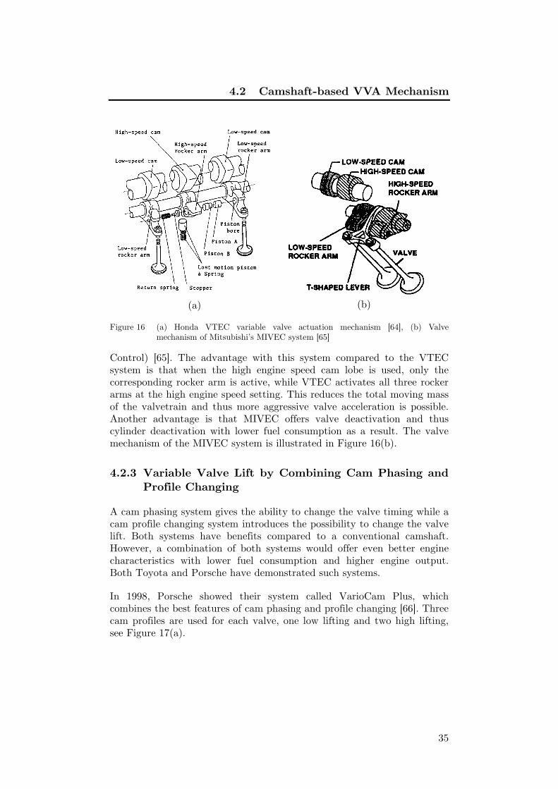
4.2 Camshaft-based VVA Mechanism
35
(a)
(b)
Figure 16 (a) Honda VTEC variable valve actuation mechanism [64], (b) Valve mechanism of Mitsubishi’s MIVEC system [65]
Control) [65]. The advantage with this system compared to the VTEC system is that when the high engine speed cam lobe is used, only the corresponding rocker arm is active, while VTEC activates all three rocker arms at the high engine speed setting. This reduces the total moving mass of the valvetrain and thus more aggressive valve acceleration is possible. Another advantage is that MIVEC offers valve deactivation and thus cylinder deactivation with lower fuel consumption as a result. The valve mechanism of the MIVEC system is illustrated in Figure 16(b).
4.2.3 Variable Valve Lift by Combining Cam Phasing and Profile Changing
A cam phasing system gives the ability to change the valve timing while a cam profile changing system introduces the possibility to change the valve lift. Both systems have benefits compared to a conventional camshaft. However, a combination of both systems would offer even better engine characteristics with lower fuel consumption and higher engine output. Both Toyota and Porsche have demonstrated such systems.
In 1998, Porsche showed their system called VarioCam Plus, which combines the best features of cam phasing and profile changing [66]. Three cam profiles are used for each valve, one low lifting and two high lifting, see Figure 17(a).
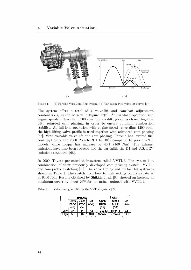
4 Variable Valve Actuation
36
(a)
(b)
Figure 17 (a) Porsche VarioCam Plus system, (b) VarioCam Plus valve lift curves [67].
The system offers a total of 4 valve-lift and camshaft adjustment combinations, as can be seen in Figure 17(b). At part-load operation and engine speeds of less than 3700 rpm, the low-lifting cam is chosen together with retarded cam phasing, in order to ensure optimum combustion stability. At full-load operation with engine speeds exceeding 1200 rpm, the high-lifting valve profile is used together with advanced cam phasing [67]. With variable valve lift and cam phasing, Porsche has lowered fuel consumption of the 2000 Porsche 911 by 18% compared to previous 911 models, while torque has increase by 40% (160 Nm). The exhaust emissions have also been reduced and the car fulfils the D4 and U.S. LEV emissions standards [68].
In 2000, Toyota presented their system called VVTL-i. The system is a combination of their previously developed cam phasing system, VVT-i, and cam profile switching [69]. The valve timing and lift for this system is shown in Table 1. The switch from low- to high setting occurs as late as at 6000 rpm. Results obtained by Shikida et al. [69] showed an increase in maximum power by about 26% for an engine equipped with VVTL-i.
Table 1 Valve timing and lift for the VVTL-I system [69]
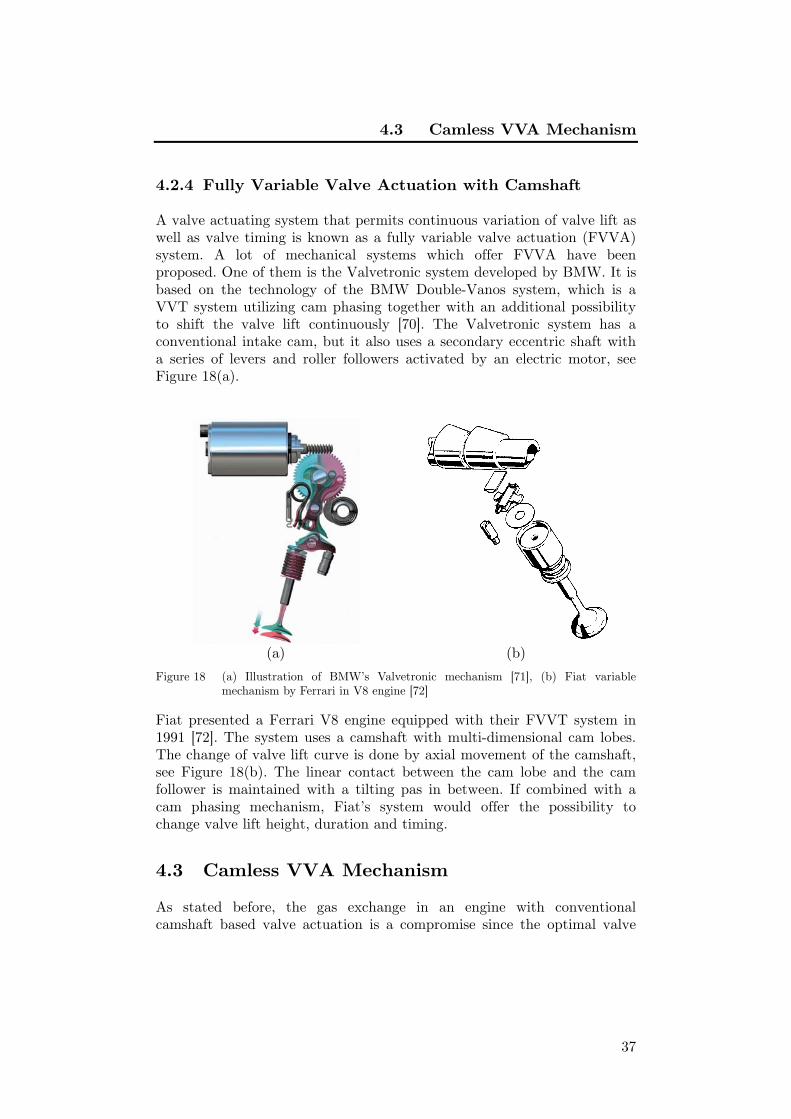
4.3 Camless VVA Mechanism
37
4.2.4 Fully Variable Valve Actuation with Camshaft
A valve actuating system that permits continuous variation of valve lift as well as valve timing is known as a fully variable valve actuation (FVVA) system. A lot of mechanical systems which offer FVVA have been proposed. One of them is the Valvetronic system developed by BMW. It is based on the technology of the BMW Double-Vanos system, which is a VVT system utilizing cam phasing together with an additional possibility to shift the valve lift continuously [70]. The Valvetronic system has a conventional intake cam, but it also uses a secondary eccentric shaft with a series of levers and roller followers activated by an electric motor, see Figure 18(a).
(a)
(b)
Figure 18 (a) Illustration of BMW’s Valvetronic mechanism [71], (b) Fiat variable mechanism by Ferrari in V8 engine [72]
Fiat presented a Ferrari V8 engine equipped with their FVVT system in 1991 [72]. The system uses a camshaft with multi-dimensional cam lobes. The change of valve lift curve is done by axial movement of the camshaft, see Figure 18(b). The linear contact between the cam lobe and the cam follower is maintained with a tilting pas in between. If combined with a cam phasing mechanism, Fiat’s system would offer the possibility to change valve lift height, duration and timing.
4.3 Camless VVA Mechanism
As stated before, the gas exchange in an engine with conventional camshaft based valve actuation is a compromise since the optimal valve

4 Variable Valve Actuation
38
timing at light loads and low engine speeds is not the same as the optimal valve timing at high engine speeds. Even though there are many camshaft-based mechanical VVA systems, they are all limited in their flexibility of individual valve and cylinder control. One way to solve this is to eliminate the camshaft. Instead the valves can be actuated by some other mechanism, such as electrical, hydraulic or pneumatic actuation. In such VVA systems the valve timing and lift are electronically controlled by a computer. The computer receives information about the current state of the engine and depending on what is desired at the moment, the control program determines the most optimal valve timings. The valve timing can in this way easily be changed from cycle to cycle, which is a big advantage in terms of combustion control.
The major advantage of camless VVA systems is the flexibility and the almost total control of the valve event. The disadvantage is that such systems are complex and expensive, and therefore mainly used by researchers in laboratories.
4.3.1 Electromagnetic Valve Actuation
Electromagnetic valve actuation (EMVA) offers great flexibility in valve timing, duration and lift. The valve actuation in this kind of systems is usually realized by different combinations of solenoids and mechanical springs. Figure 19(a) shows a cross-section of GM’s electro-mechanical valve actuator. The valve is equipped with a plunge and placed inside a housing containing a permanent magnet and an electromagnet. When the valve is in its closed position, Spring A is compressed and the valve is held in place by the permanent magnet. To open the valve Coil A has to be activated and cancel the magnetic field of the permanent magnetic pole. This allows the spring force exerted by Spring A to accelerate the valve. As the valve moves towards its lower position, the plunger is attracted by the other permanent magnetic pole and Spring B is compressed. The valve closing event is done in a reversed procedure compared to the valve opening event [73].
Figure 19(b) displays a typical valve lift profile achieved with an electromagnetic valve actuating system. Compared to a conventional valve lift, the electromagnetic valve lift profile has a much steeper valve-opening ramp which promotes better cylinder filling at low and medium engine speeds.
Theobald et al. [74] state that GM’s electromagnetic system has lower energy consumption than a standard camshaft driven valve train at the

4.3 Camless VVA Mechanism
39
(a)
(b)
Figure 19 (a) Cross-section of GM’s electromechanical valve actuator [74], (b) A typical valve lift profile for an electromagnetic valve train [75]
same speed. A disadvantage with GM’s system is that the valve seating velocity is unacceptably high with high noise levels as a result. A solution to such valve seating problems has been proposed by Mianzo et al. [76] where the valve is slowed down by resistance induced by the valve stem entering a fluid-filled cavity. Because of the increased resistance, a soft seating of the valve head is achieved.
4.3.2 Electrohydraulic Valve Actuation
Another way to achieve camless valve operation is by electrohydraulic valve actuation (EHVA). Electrohydraulic valve actuators convert fluid pressure into motion in response to a signal. Schechter et al. [77] describes an EHVA system for variable control of engine valve timing, lift and velocity. The system does not use cams or springs, instead the valves are both opened and closed by hydraulic force. Throughout the valve acceleration, the potential energy of the compressed fluid is transformed into kinetic energy of the valve. During deceleration the energy of the valve motion is returned to the fluid. Figure 20(a) illustrates Ford’s electrohydraulic valve train actuation concept and Figure 20(b) shows the lift profile for the system in question. The working principal of the valve train is that when the vale is in its closed position, the high-pressure solenoid is opened and the high-pressure fluid is allowed to enter the volume above the valve. The pressure above and below the valve piston is

4 Variable Valve Actuation
40
equal but since the area on the upside of the valve piston is larger, the net hydraulic force is directed downward and therefore the valve opens. As the valve moves towards its lower position, the high pressure solenoid closes which results in a cut-off of the high pressure supply. Even though the pressure above the valve piston decreases, the valve keeps on going due to its momentum. As the valve moves towards its end position the low pressure check valve opens and low pressure fluid enters the volume in such way that the valve decelerates until it stops at the desired valve lift. During the dwell-period, both solenoids and check valves are closed and thus the valve is prevented from returning since hydraulic pressure acts on both sides of the valve piston. The valve closing event is initiated by the activation of the low pressure solenoid. The valve pushes the fluid back to the low pressure source while returning to its closed position. As the valve approaches its closed position, the high pressure check valve opens and the valve opens and the valve starts to slow down.
(a) (b) Figure 20 Illustration of Ford’s electrohydraulic camless valve train; (a) Cross-section of
the electrohydraulic valve actuator, (b) The lift profile of the electrohydraulic valve train [77]
Lotus has been developing an electrohydraulic valve actuation system since the early 1990’s. The system is known as Lotus active valve train (AVT). It consists of a hydraulic piston attached to the engine valve which moves inside a hydraulic cylinder. The movement of the valve is controlled via fluid flow either above or below the actuator piston, and the fluid flow is in turn controlled by a high-speed servo valve [78]. Figure 21(a) displays a Lotus AVT system mounted on a cylinder head.
Figure 21(b) illustrates the hydraulic circuit of the research AVT system. The valve profile is continuously monitored by a linear displacement

4.3 Camless VVA Mechanism
41
transducer (LDT), which makes valve profile correction from cycle-to-cycle possible. The AVT system has fully flexible control of the entire valve event. The desired vale profile is entered in a control program and with the help of the LDT the valve is operated according to the desired valve lift profile. The system permits individual valve control and can operate different valve lift profile on different valves. In addition to this, the system is capable of opening a valve more than once during an engine cycle [78, 79]. Valve profiles of varying shapes, such as polynomial, triangular or trapezoidal, are easily generated by an engine valve lift profile generator capable of storing up to 256 individual vale lift profiles [80].
(a) (b)Figure 21 Lotus research AVT system; (a) The electrohydraulic valve actuator, (b)
Schematic of the hydraulic circuit used in the research AVT system [78].
The aforementioned system is only intended for research and it is not at all suitable for mass-produced engines. The reason is the technology used is extremely expensive and the high-speed servo does not allow controlled valve velocities with sufficient accuracy above engine speeds of 4000 rpm. Lotus and Eaton are collaborating to develop a production ready version of AVT and they expect to market the product in the 2008-9 timeframe [81]. However, at the time of writing, no updated information about the status of the production AVT system can be found.
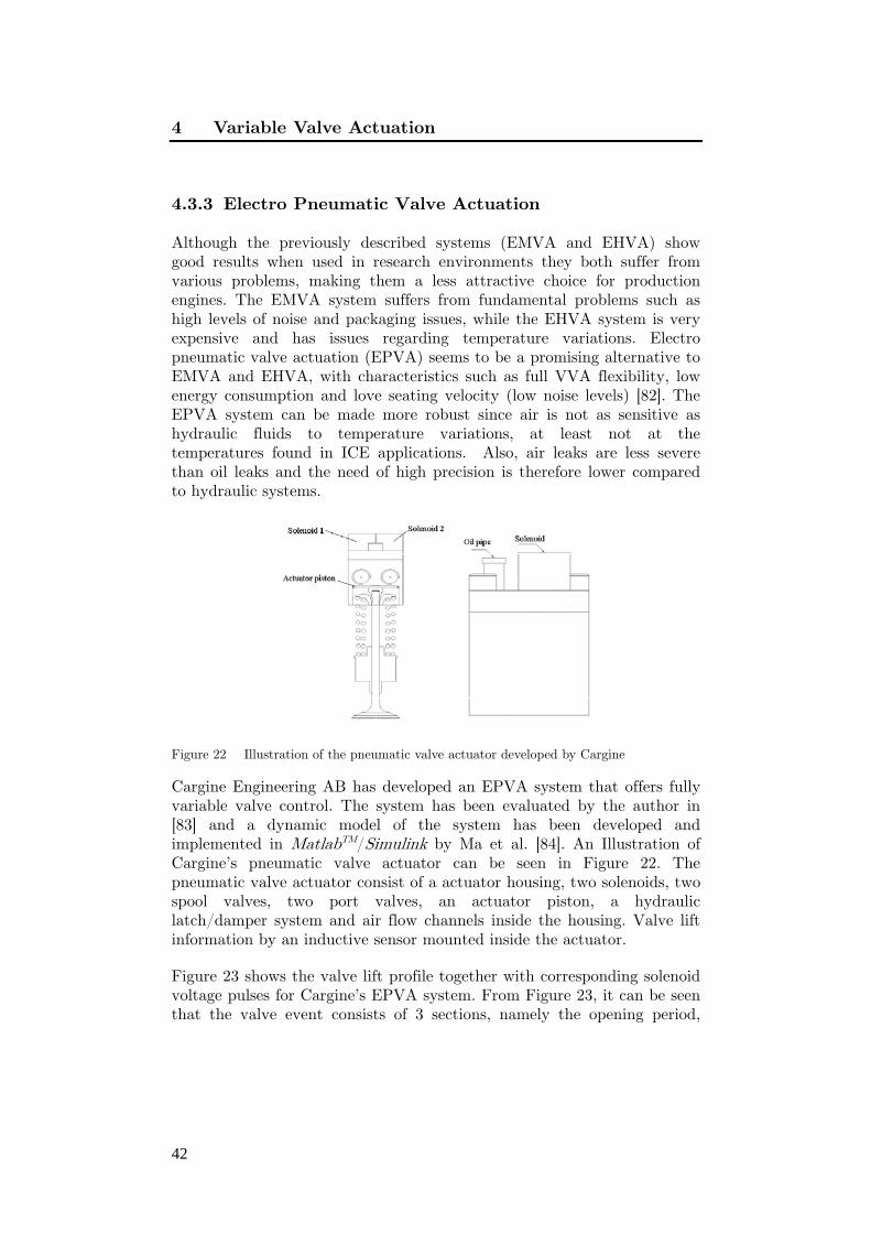
4 Variable Valve Actuation
42
4.3.3 Electro Pneumatic Valve Actuation
Although the previously described systems (EMVA and EHVA) show good results when used in research environments they both suffer from various problems, making them a less attractive choice for production engines. The EMVA system suffers from fundamental problems such as high levels of noise and packaging issues, while the EHVA system is very expensive and has issues regarding temperature variations. Electro pneumatic valve actuation (EPVA) seems to be a promising alternative to EMVA and EHVA, with characteristics such as full VVA flexibility, low energy consumption and love seating velocity (low noise levels) [82]. The EPVA system can be made more robust since air is not as sensitive as hydraulic fluids to temperature variations, at least not at the temperatures found in ICE applications. Also, air leaks are less severe than oil leaks and the need of high precision is therefore lower compared to hydraulic systems.
Figure 22 Illustration of the pneumatic valve actuator developed by Cargine
Cargine Engineering AB has developed an EPVA system that offers fully variable valve control. The system has been evaluated by the author in [83] and a dynamic model of the system has been developed and implemented in MatlabTM/Simulink by Ma et al. [84]. An Illustration of Cargine’s pneumatic valve actuator can be seen in Figure 22. The pneumatic valve actuator consist of a actuator housing, two solenoids, two spool valves, two port valves, an actuator piston, a hydraulic latch/damper system and air flow channels inside the housing. Valve lift information by an inductive sensor mounted inside the actuator.
Figure 23 shows the valve lift profile together with corresponding solenoid voltage pulses for Cargine’s EPVA system. From Figure 23, it can be seen that the valve event consists of 3 sections, namely the opening period,

4.3 Camless VVA Mechanism
43
dwell period and closing period. The opening period starts with the activation of Solenoid 1 (S1) which in turn pushes the corresponding spool
Figure 23 A typical valve lift profile achieved with Cargine’s EPVA system. Below the valve lift curve, a solenoid action chart can be seen. Observe that the system delays are excluded from the solenoid chart [84].
valve. The new position of the spool valve now permits pressurized air to enter the actuator cylinder. The pressurized air pushes the actuator piston and since the valve is in direct contact with the actuator piston, it starts to open. Solenoid 2 (S2), is activated in order to stop the air charging of the actuator cylinder and the time difference between activation of S1 and activation of S2, δ1, therefore determines the valve lift. The pressurized air expands inside the actuator cylinder until it balances with the valve spring force. At the end of the opening period, the hydraulic latch is activated and the valve is prevented from returning. The hydraulic latch is active during the entire dwell period. When S1 is deactivated, the latch is disabled which in turn starts the air discharge from the actuator cylinder and the valve starts its closing period. The time difference between the deactivation of S2 and S1, δ2, must always be positive to prevent a second air filling of the actuator cylinder since this would trigger a second valve lift event. At the end of the closing period (about 3 mm before the end of valve lift) the hydraulic damper is activated, and starts to slow down the valve. In the interval 1.0 to 0.0 mm, the seating velocity is constant with a magnitude of approximately 0.5 m/s. thereby the damper ensures a soft-seating with low level of noise as a result.

4 Variable Valve Actuation
44
Cargine is not alone in this file, however, it seems as their product is the one most likely to reach the market in a near future. Johnson et al. [85] describes a free-piston engine using pneumatically operated valves. However, the valves in the engine described are not of the conventional type. Instead of poppet valves, the engine uses spool valves. As the piston approaches the end of its stroke, the pressure is built up in the cylinder and pressurized gas is conducted to the valves through fluid lines, making the spool valves move in the desired direction. The system does not admit any type of control over the valve event.
Richeson et al. [86] presents an electronically controlled pneumatically powered transducer for use as a valve actuator in an ICE. The transducer contains a piston which can easily be coupled to an engine valve. The piston is displayed by pressurized air controlled by permanent magnet control valves. At the start of the opening period, the permanent magnet is temporarily neutralized making the control valve to open. This leads to a filling of the cylinder above the piston, thus pushing it to its opposite end position. Then the piston reaches the end of its stroke, the control valve is closed by the permanent magnet and the pressurized air in the cylinder keeps the piston at its end position and the dwell period has been initiated. To start the closing period, the permanent magnet below the piston is neutralized which admits opening of the control valve and results in a subsequent charging of the cylinder from underneath the piston. The system is equipped with a soft-seating mechanism using air as cushion. The system can be described as a VVT system, since the valve timings can be controlled as desired, but the lack of valve lift control disqualifies it as an FVVA system. Gould et al. [87] tested the system described above, implemented in a test engine, with satisfying results considering
Figure 24 Valve lift profile comparison between cam driven and pneumatic actuator driven valves [87]

4.4 Valve Strategies Enabled by FVVA
45
that no optimization of the implementation was done. Figure 24 shows the three valve lift profiles with constant vale lift duration at three different engine speeds for the EPVA system in question.
In 2005, Watson et al. [142] showed results achieved from simulations of a pneumatic valve actuation system. However, no prototype has been demonstrated at the time of writing.
4.4 Valve Strategies Enabled by FVVA
With FVVA, unlimited possibilities to investigate effects of various valve timings arise. For instance, by closing the inlet vale late (a number of degrees ABDC) the effective compression ratio is changed, with a second opening of the exhaust valve ATDC “internal” exhaust gas recirculation (EGR) is achieved, deactivation of valves in order to alter the in-cylinder flow etc. some of the most common valve strategies enabled by FVVA will be discussed in the forthcoming sections.
4.4.1 Negative Valve Overlap
For a very long time EGR has been used in order to reduce the NOx exhaust emissions. The exhaust gases recirculated to the intake manifold dilutes the air/fuel charge which results in a reduced peak combustion temperature and thereby the temperature-dependent NOx emissions will be lowered. However, with some combustion concepts the residual gases are used for a completely different reason. For instance, HCCI (Homogeneous Charge Compression Ignition) is a combustion concept where the air/fuel-mixture self-ignites and it depends to a great extent on the charge temperature. One way to increase the charge temperature is to dilute it with hot burned residual gases. This can be achieved with a valve strategy known as negative valve overlap (NVO).
With NVO, the exhaust valve closes somewhere before TDC and a large amount of hot residual gases are then trapped in the cylinder. The residuals are then compressed during the rest of the exhaust stroke and then expanded during the intake stroke until they reach ambient conditions when the inlet valve opens. It is important to open the inlet vale at the right moment, since an early IVO leads to a blowdown of residuals through the inlet port, with unnecessary pumping losses. On the other hand, late IVO means that the residuals will be expanded beyond ambient conditions and vacuum is created which costs work. Ideally, exhaust valve closing (EVC) and IVO should be mirrored with respect to TDC, i.e. the period from TDC when the intake and exhaust valves are

4 Variable Valve Actuation
46
(a) (b) Figure 25 (a) Illustration of valve profiles for standard engines (solid lines) and for
engines utilizing different degrees of NVO (dashed lines), (b) Pressure trace from an engine running with HCCI combustion and a NVO of 100 CAD
closed during gas exchange should be almost equal. Figure 25(a) shows the valve profile for an engine with conventional valve timing together with valve lift profiles for two different degrees of NVO. Figure 25(b) show the in-cylinder pressure from an engine run with NVO HCCI.
Numerous researchers have shown results involving NVO in their studies over the past decade. The NVO strategy was first published by Willand et al.[89] in 1998, however ni results were presented. Among the first to show results from NVO HCCI was Kontarakis et al. [90] in 2000.
4.4.2 Rebreathe Strategy
Another way to retain residuals in the cylinder is by exhaust rebreathing. Instead of trapping the residuals in the cylinder and the compressing them, the exhaust gases are expelled through the exhaust or inlet port, after which they are brought back into the cylinder during a part of the intake stroke. A rebreathing strategy can be achieved in a number of ways and four of the will be explained with references to Figure 26.
Figure 26(a) shows the valve timings for exhaust port recirculation. In this type of strategy, the exhaust valve remains open during the entire exhaust stroke and closes during the intake stroke. In this way exhausts are first expelled through the exhaust port, after which they are brought back to the cylinder. The inlet valve opens first after the exhaust valve closes in order to prevent mixing between the reinducted exhausts and the fresh charge, and thereby secure a stratified charge mixture [91]. Results achieved by engines running with this kind of rebreathing strategy have been shown by, amongst others, Kaahaaina et al. [92].
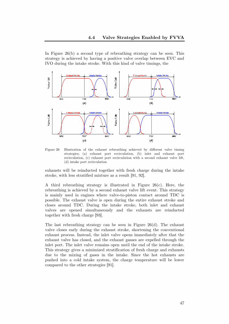
4.4 Valve Strategies Enabled by FVVA
47
In Figure 26(b) a second type of rebreathing strategy can be seen. This strategy is achieved by having a positive valve overlap between EVC and IVO during the intake stroke. With this kind of valve timings, the
Figure 26 Illustration of the exhaust rebreathing achieved by different valve timing strategies; (a) exhaust port recirculation, (b) inlet and exhaust port recirculation, (c) exhaust port recirculation with a second exhaust valve lift, (d) intake port recirculation
exhausts will be reinducted together with fresh charge during the intake stroke, with less stratified mixture as a result [91, 92].
A third rebreathing strategy is illustrated in Figure 26(c). Here, the rebreathing is achieved by a second exhaust valve lift event. This strategy is mainly used in engines where valve-to-piston contact around TDC is possible. The exhaust valve is open during the entire exhaust stroke and closes around TDC. During the intake stroke, both inlet and exhaust valves are opened simultaneously and the exhausts are reinducted together with fresh charge [93].
The last rebreathing strategy can be seen in Figure 26(d). The exhaust valve closes early during the exhaust stroke, shortening the conventional exhaust process. Instead, the inlet valve opens immediately after that the exhaust valve has closed, and the exhaust gasses are expelled through the inlet port. The inlet valve remains open until the end of the intake stroke. This strategy gives a minimized stratification of fresh charge and exhausts due to the mixing of gases in the intake. Since the hot exhausts are pushed into a cold intake system, the charge temperature will be lower compared to the other strategies [91].

4 Variable Valve Actuation
48
4.4.3 Atkinson/Miller Cycle
The Atkinson cycle was invented in the 1880s by a British engineer named James Atkinson. The main feature of the Atkinson cycle is that the expansion stroke is longer than the compression stroke, thus converting a greater portion of the energy from heat to useful mechanical energy with a greater efficiency as a result. In 1886 Atkinson presented the “cycle engine” which utilized the Atkinson cycle. The disadvantage with the cycle engine, however, was that the mechanisms for having different stroke lengths were complex, with an increased risk of failure and increased friction losses, as a result. Because of this, in combination with expiration of Nicolaus Otto’s patent on the four-stroke cycle in 1890, the cycle engine did not survive for very long [94].
In 1954, Ralph Miller, patented the so called “Miller cycle” which is a modified version of the Atkinson design [95]. The main idea with the Miller cycle is that the difference between compression ratio and expansion ratio is achieved by closing the inlet valve past the end of the intake stroke, rather than being a geometrical difference between compression and exhaust stroke. In this way a part of the charge inhaled during the intake stroke is expelled through the inlet port until the inlet valve closes, whereupon the compression starts. However, the decreased amount of charge leads to a lower maximum power. This can be compensated by the use of a supercharger. The Miller strategy can also be achieved by closing the inlet valve before the end of the intake stroke.
Luria et al. [96] presented in 1982 a concept called the Otto-Atkinson engine which operates as a hybrid cycle between the conventional Otto cycle and the Atkinson cycle. Even though “Atkinson” is referred to in the name of the concept, it utilizes the late IVC as described by Miller. Toyota utilizes the Otto-Atkinson concept in their hybrid vehicle named Prius [97].

49
Chapter 5
5 Modeling the Pneumatic Hybrid
In this chapter the different model of the pneumatic hybrid concept will be presented. The pneumatic hybrid engine is modelled in GT-Power while the complete pneumatic hybrid vehicle is modelled in Matlab™/Simulink. In the following sub-sections both models will be thoroughly described.
5.1 Pneumatic Hybrid Engine Modeling in GT-Power
The main intent with the pneumatic hybrid engine model is to further explore its potential and characteristics. The experimental part of the thesis shows that different factors, like for instance tank valve head diameter and valve timings, play an important role in the overall pneumatic hybrid engine performance. While it is time consuming to change the tank valve head diameter on a real engine, it can be done within seconds on a computer model. Therefore a real engine based computer model can serve as a tool in order to more easily investigate different parameters and how they affect the performance of the pneumatic hybrid engine. With a model of the experimental engine, problems like malfunction of the tank valve setup at high pressures can be avoided. Also, a model introduces the possibility to investigate important parameters such as valve timings and valve diameters with ease.
The pneumatic hybrid engine modeling was conducted in GT-Power. GT-Power is an engine simulation tool commonly used by researchers as well as engine and vehicle producers. It is based on one-dimensional gas dynamics and is capable of simulating the gas flow and heat transfer in the pipes, cylinder and other components of an ICE. GT-Power also offers specialized features needed for ICE modeling such as valve actuation (both cam-driven and VVA), fuel injection and turbocharging.
The base engine model, provided by Scania is based on the same base engine configuration as the one used during the engine testing described in

5 Modeling the Pneumatic Hybrid
50
this thesis. However, since only one cylinder was used during the experimental study, the base model had to be modified. The base engine model was equipped with camshaft driven valves which were replaced with a variable valve actuating system equivalent to the one used on the experimental engine. A pressure tank was also added to the model and connected to one of the inlet ports of the engine. The original piston with a bowl was exchanged for a flat piston as used in the experimental engine. All piping was also modified so that it reproduced the piping used on the experimental engine. The final model can be seen in Figure 27.
Figure 27 GT-Power model of the Scania single-cylinder engine
The addition of new parts to the model introduced new unknown parameters such as heat transfer coefficient for the pressure tank and friction losses in the metallic tubing connecting the pressure tank to the engine. Since these new parameters were unknown, great care was taken in tuning them. Therefore the model was validated against experimental engine data and the validation will be presented in sections 7.1.4 and 7.2.3.
An important aspect of model validation is that the relative error between measured data and simulated data should not exceed a certain value in order to classify the model as “accurate”. Morrissey et al. [98] showed results where the error ranges up to 30% while Westin et al. [99] showed steady-state operating points with an accuracy of 5-10%. The aim of the model calibration in the project behind this thesis was to ensure that for steady-state operating points the error would not exceed 5% for as many model parameters as possible.

5.2 Pneumatic Hybrid Vehicle Modeling in Simulink/Matlab™
51
5.2 Pneumatic Hybrid Vehicle Modeling in Simulink/Matlab™
One of the most important questions regarding pneumatic hybridization that needs to be addressed is how it affects the fuel consumption. For this purpose a pneumatic hybrid vehicle is needed. Due to a limited resources, conversion of a real vehicle to work as a PHV was completely out of reach. This motivated the development of a PVH model.
In Paper IV and Paper V the model used was based on a city bus, which is motivated by the fact that city buses are mainly operated in cities where the driving cycles are characterized by frequent stops and engine idling. Frequent stops leads to frequent braking events during which the kinetic energy of the vehicle is converted to thermal energy in the friction brakes, and engine idling consumes energy without performing any positive work. With pneumatic hybridization, this otherwise wasted brake energy can be captured and stored for use at a later time while energy losses during idling can to a great extent be avoided. All this leads to reductions in fuel consumption and exhaust emissions. Another reason for choosing a city bus as a subject for the model simulations is that the experimental part of the project was conducted on a heavy-duty engine and therefore it is quite natural to model a vehicle of that nature.
The PHV model used in the thesis was developed in Matlab™/Simulink. The base vehicle model was developed by the Department of Industrial Engineering and Automation (IEA) at Lund University and has been thoroughly described in [100].
It was based on a typical vehicle for personal transport equipped with an electric hybrid powertrain. The vehicle utilized a 1.5 liter diesel engine based on maps obtained experimentally. Since the purpose of the studies presented in Paper IV and Paper V was to evaluate the pneumatic hybrid powertrain implemented in a city bus, the model needed some modifications.
The original ICE model was based on a 1.5 liter compression ignited (CI) 4-cylinder engine, while the city bus engine was based on a 12L direct injected (DI) 6-cylinder engine. Therefore, the original ICE model was replaced by an ICE model based on data from a GT-Power model of a Scania D12 engine designed by Scania and validated by Svensson [101].

5 Modeling the Pneumatic Hybrid
52
All electric-hybrid related components were removed and replaced by pneumatic hybrid components. The pneumatic hybrid engine performance maps are generated in the previously described GT-Power model.
Vehicle specific data like weight, frontal area, maximum torque and power, were updated with suitable data for the chosen vehicle. The most significant vehicle data can be seen in
Table 3. The auxiliary power demand of 4 kW is a mean value for the entire Braunschweig drive cycle and has been chosen in accordance with [102].
Table 2 Vehicle data for the simulated city bus.
Total Vehicle Weight 15000 kg Wheel Radius, rw 0.517 m Air Resistance, Cd 0.75 Rolling Resistance, Cr 0.008 Frontal Area 7.5 m2 Auxiliary power demand 4 kW Maximum Vehicle Speed 80 km/h Pressure Tank Volume 40 liter Starting tank pressure 23.7 bar Lower tank pressure limit 8 bar Upper tank pressure limit 27 bar
Figure 28 and Figure 29 show the top level of the pneumatic hybrid bus model and the pneumatic hybrid subsystem, respectively.
The top level of the pneumatic hybrid, shown in Figure 28, contains both a conventional and the pneumatic hybrid driveline. The reason is that in this way performance data obtained for the pneumatic hybrid vehicle can at all times be compared to corresponding data for a conventional vehicle undergoing the same driving conditions.
The pneumatic hybrid subsystem, shown in Figure 29, mainly consists of blocks representing the two relevant modes of engine operation, i.e. compressor mode and air-motor mode. In these mode specific blocks, the engine maps obtained with GT-Power are located. The control strategy for choosing the proper mode of operation and controlling the way they are operated in is quite simple. The blocks representing the modes of engine operation accepts a demanded drive/brake torque as input. The torque is then evenly divided amongst the cylinders. Mainly, the cylinders are operated in two-stroke mode. However, if the torque falls out of the
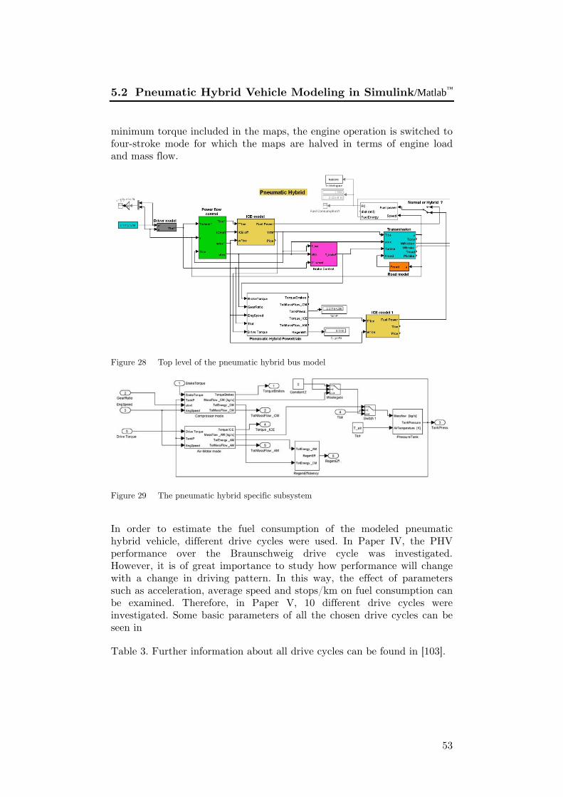
5.2 Pneumatic Hybrid Vehicle Modeling in Simulink/Matlab™
53
minimum torque included in the maps, the engine operation is switched to four-stroke mode for which the maps are halved in terms of engine load and mass flow.
Figure 28 Top level of the pneumatic hybrid bus model
Figure 29 The pneumatic hybrid specific subsystem
In order to estimate the fuel consumption of the modeled pneumatic hybrid vehicle, different drive cycles were used. In Paper IV, the PHV performance over the Braunschweig drive cycle was investigated. However, it is of great importance to study how performance will change with a change in driving pattern. In this way, the effect of parameters such as acceleration, average speed and stops/km on fuel consumption can be examined. Therefore, in Paper V, 10 different drive cycles were investigated. Some basic parameters of all the chosen drive cycles can be seen in
Table 3. Further information about all drive cycles can be found in [103].

5 Modeling the Pneumatic Hybrid
54
Figure 30 illustrates vehicle speed as a function of time for two drive cycles, the New York bus drive cycle and the FIGE (Forschungsinstitut Gerausche und Erschutterungen) drive cycle. The New York bus cycle is characterized by a low maximum and average speed together with a large number of stops/km. the FIGE drive cycle consists of three parts,
Table 3 Basic parameters of the different drive cycles used in present study (Brauns=Braunschweig, CBD=Central Business District, OC=Orange County, CSC=City Suburban Cycle, FIGE=Forschungsinstitut Gerausche und Erchutterungen, HD-UDDS=Heavy-Duty Urban Dynamometer Driving Schedule, NY=New York)
Cycle CBDNY Bus
NY Comp.
Manh. Bus
OC Bus
Brauns. Bus FIGE CSC
Japan JE05
HD-UDDS
Time [s] 560 600 1029 1089 1909 1740 1800 1700 1829 1060 Distance
[km] 3.29 0.99 4.03 3.32 10.53 10.87 29.49 10.75 13.89 8.94 Avg. Speed [km/h] 21.1 5.94 14.11 10.99 19.85 22.5 58.98 22.77 27.33 30.32 Max Speed [km/h] 32.2 49.6 57.94 40.88 65.39 58.2 91.1 70.56 87.6 93.34 Idle [%] 17.7 65.5 33.14 35.98 21.27 25.34 0 23.29 25.19 33.27
Max Acc. [m/s^2] 0.89 0.31 2.07 0.22 1.82 2.42 3.83 1.14 1.59 1.96
Max Decl.
[m/s^2] 2.24 0.22 1.96 0.27 2.29 3.58 4.03 1.77 1.83 2.07 Stops 14 12 21 21 32 30 0 14 15 15
Stops/km 4.25 12.1 5.21 6.32 3.04 2.76 0 1.3 1.08 1.68
(a) (b) Figure 30 Vehicle speed as a function of time during two different drive cycles; (a) New
York Bus drive cycle, (b) FIGE drive cycle.
0 100 200 300 400 500 6000
10
20
30
40
50
Time [s]
Ve
hic
le S
pe
ed
[km
/h]
0 500 1000 15000
20
40
60
80
100
Time [s]
Ve
hic
le S
pe
ed
[km
/h]

5.2 Pneumatic Hybrid Vehicle Modeling in Simulink/Matlab™
55
including city, rural and motorway driving where the duration of each part is 600 seconds.
Figure 31 shows the mean and maximum accelerations/decelerations, respectively, for all drive cycles. They illustrate the degree of aggressiveness of the different drive cycles. For instance, the CBD drive cycle has the highest mean acceleration and deceleration which together with a relatively high maximum acceleration and deceleration, makes this drive cycle quite aggressive. The New York and Manhattan bus drive cycles both have very low mean and maximum acceleration/deceleration which makes them the least aggressive of all chosen drive cycles.
(a) (b)
Figure 31 Acceleration and deceleration during the different drive cycles; (a) Mean acc/dec, (b) Maximum acc/dec.
Figure 32 Mean and maximum speed during different drive cycles
Figure 32 illustrates mean and maximum speed during the chosen drive cycles. The bus cycles show a quite low mean speed which can be explained by the high number of stops/km compared to the non-bus cycles. The FIGE drive cycle shows the highest mean speed of all drive cycles, mainly due to the fact that this drive cycle contains a motorway-driving section.
-2
-1
0
1
2
Acc
eler
atio
n [
m/s
2]
CBD
NYbus
NYcom
p
Man
h
OCbus
BraunS
FIGE
CSCJE
05
UDDS
Mean AccelerationMean Deceleration
-6
-4
-2
0
2
4
6
Acc
eler
atio
n [
m/s
2]
CBD
NYbus
NYcom
p
Man
h
OCbus
BraunS
FIGE
CSCJE
05
UDDS
Max AccelerationMax Deceleration
0
20
40
60
80
100
Sp
eed
[km
/h]
CBD
NYbus
NYcom
p
Man
h
OCbus
BraunS
FIGE
CSCJE
05
UDDS
Mean SpeedMax Speed

56
Chapter 6
6 Experimental Setup
During the project summarized in present thesis, three different test rigs have been used. The reason of switching between these test rigs was that the pneumatic hybrid project did not have a dedicated engine and the used test rigs had limited time slots available, which made moving between different test rigs inevitable.
6.1 Test Engines
All three test rigs used in the pneumatic hybrid project were equipped with engines originating from Scania D12 and D13 Diesel engines. However, each engine is modified in some way to fit the corresponding application. In following sub-sections, each engine will be described along with the necessary modifications.
6.1.1 Paper I
The engine used in Paper I was a single-cylinder engine originating from a six cylinder Scania D12 Diesel engine. The standard version of this engine
(a) (b)
Figure 33 (a) The single-cylinder Scania diesel engine used in Paper I; (b) The pneumatic valve actuators mounted on the Scania cylinder head.

6.1 Test Engines
57
has 4 engine valves per cylinder. A picture of the engine can be seen in Figure 33(a).
The standard Scania D12 engine uses a piston with a bowl in its crown. In the pneumatic hybrid project the standard piston has been exchanged for a flat piston in order to increase the piston clearance and thus avoid any valve-to-piston contact when using the pneumatic VVA system. The same flat piston has been used in Paper I and Paper II. Some engine specifications can be found in Table 4.
Table 4 Geometric properties of the Scania D12 Diesel engine.
Displaced Volume per Cylinder 1966 cm3 Bore 127.5 mm Stroke 154 mm Connecting Rod Length 255 mm Number of Valves 4 Compression Ratio 18:1 Piston type Flat Inlet valve diameter 45 mm Exhaust valve diameter 41 mm Valve Timing Variable Piston clearance 7.3 mm
The standard camshaft was removed and the engine valves are actuated by the pneumatic VVA system described in Section 4.3.3. Figure 33(b) shows the pneumatic valve actuators mounted on the Scania cylinder head. The same setup has been used in Paper I, Paper II, Paper III and Paper VII. The maximum valve lift height has been limited to 7 mm in order to avoid valve-to-piston contact and thus prevent engine failure. In Table 5, some valve operating parameters are shown. The standard valve springs have been exchanged for less stiff springs in order to reduce the energy required to operate the valves.
Since the intent with the project was to study pneumatic hybrid engine operation, a pressure tank was added to the experimental setup. The pressure tank is an AGA 50 liter pressure tank suitable for pressures up to 200 bar. It is connected to the cylinder head by metal tubing suitable for pressures up to 60 bar and temperatures exceeding 500°C. The size of the tank was selected based on availability rather than optimality. The engine has two separated inlet ports and therefore it was suitable to connect one of them to the tank since there will be no interference between the intake air and the compressed air. One of the inlet valves was therefore converted to operate as a tank valve. The purpose of the tank valve is to

6 Experimental Setup
58
Table 5 Valve operating parameters
Inlet valve diameter 45 mmTank valve diameter 16 mmInlet valve supply pressure 4 bar Exhaust valve supply pressure 6 bar Hydraulic brake pressure 4 bar Inlet valve spring preloading 100 N Tank valve spring preloading 340 N Maximum valve lift 7 mm
control the air flow to and from the pressure tank. In order to open the tank valve at high in-cylinder pressures some modifications of the tank valve has to be introduced. The valve head diameter was decrease from 45 mm to 16 mm. Also the tank valve spring preloading had to be modified and was changed from 100 N to 340 N in order to keep the tank valve completely closed for tank pressures up to 25 bar. Due to the increased valve spring preloading, the supply pressure to the tank was increased compared to the corresponding pressure for the inlet valve in order to ensure proper valve actuator operation.
The exhaust valves were deactivated throughout the study presented here because no fuel was injected and thus there was no need for exhaust gas venting.
6.1.2 Paper II and Paper III
The engine used in Paper II and Paper III was an in-line six cylinder Scania D12 Diesel engine. In this setup one of the cylinders was modified for pneumatic hybrid engine operation, while remaining cylinders were intact, see Figure 34.
Experiments performed in Paper I showed that a tank valve head diameter of 16 mm lead to considerable compressed air flow restrictions across the valve. In order to avoid this, a pneumatic valve spring was designed and will be more thoroughly described in the following section. The tank valve head diameter was therefore changed to 28 mm. Both tank valve geometries can be seen in Figure 34(b) and TABLE XXX displays some valve geometric properties and operating parameters. The original metal tubing which connects the pressure tank to the cylinder head has an inner diameter of 25 mm, which is smaller than the diameter of the new tank valve. Therefore, in order to eliminate the metal tubing as

6.1 Test Engines
59
a potential bottleneck on account of air flow choking, the diameter of the tubing was doubled.
(a) (b) Figure 34 (a) The modified Scania D12 Diesel engine. The operating cylinder is to the
left in the picture; (b) Picture illustrating the difference between the “small tank valve” (Ø = 16 mm) and the “large tank valve” (Ø = 28 mm).
Table 6 Valve geometric properties and operating parameters.
Inlet valve diameter 45 mm Tank valve diameter 16 and 28 mm Inlet valve supply pressure 4 bar Tank valve supply pressure 6 bar Hydraulic brake pressure 4 bar Inlet valve spring preloading 100 N Maximum valve lift 7 mm
6.1.3 Paper VI
The engine used in the study presented in Paper VI was an in-line six-cylinder Scania D13 Diesel engine, see Figure 35. Also in this experimental setup one of the cylinders was modified for pneumatic hybrid operation while the remaining cylinders where intact.
The standard Scania D13 diesel engine uses a piston with a bowl in its crown. In previous setups, the standard piston was exchanged for a flat piston in order to increase the piston clearance and thus avoid any valve-to-piston contact when using the pneumatic VVA system. However, since current system is equipped with a direct injection system, the bowl needs to remain intact as much as possible in order to secure a satisfying combustion. The only modification done to the piston crown was the addition of a valve pocket directly underneath the tank valve since it

6 Experimental Setup
60
Figure 35 The modified Scania D13 Diesel engine. The operating cylinder is to the left in the picture
usually needs to be open even at TDC and the low piston clearance would not allow this. Some engine specifications can be found in Table 7.
Table 7 Geometric properties of the Scania D13 diesel engine.
Displaced Volume/Cylinder 2100 cm3 Bore 130 mm Stroke 160 mm Connecting Rod Length 255 mm Number of Valves 4 Compression Ratio 17.2 Piston type Bowl Inlet valve diameter 45 mm Tank valve diameter 28 Piston clearance 0.9 mm
Some of the experiments described in Paper VI required steady-state tank pressure and for this purpose a pressure relief valve was connected to the tank. In this way two tank flows are achieved, one into the tank from the engine and one out from the tank to the surroundings. By matching the outflow against the inflow, different degrees of steady state tank pressure can be achieved. The greater the valve opening angle the higher the flow out from the tank becomes with a lower steady-state tank pressure as a result. The relief valve is connected to an electronically controlled actuator of type AKM 115S F132 by Sauter Components.

6.2 Pressure compensated tank valve
61
6.2 Pressure compensated tank valve
In Paper I, the tank valve head diameter was decreased from the original size of 41 mm to 16 mm in order to ensure proper valve operation at all time. The reason is that for a large valve is becomes difficult to open against high in-cylinder pressures due to an unbalanced force distribution that arises due the negative difference in actuator piston and tank valve head diameter. Also the spring preloading was changed from 100 N to 340 N in order to keep the tank valve completely closed at tank pressures up to 25 bars. Both modifications lead to some complications. The reduced valve diameter increases the flow restrictions across the valve while the increased spring preloading will affect the pneumatic valve actuator energy consumption. The later is only of importance in a real vehicle where the actuator has to be feed with pressurized air from a compressor.
In an attempt to avoid the pressure losses over the tank valve, an in-house designed pneumatic valve spring was developed and replaced the conventional tank valve spring. Figure 36 displays a simple cross-section illustration of the pneumatic valve spring arrangement mounted on the cylinder head and the concept will be explained with references to Figure 36. The numbers in brackets found in the description below, refer to the numbers displayed in Figure 36.
The pneumatic valve spring is constructed in such way, that it uses the tank pressure to keep the valve closed. A cylinder (1) is placed on top of the cylinder head (4), with the tank valve (3) in the center of the cylinder. The cylinder is sealed at the bottom the cylinder head and on top the cylinder is sealed against the valve spring retainer (2). The space between the bottom sealing and the tank valve spring retainer is the pneumatic spring and it is connected to the tank valve port (6) and thus to the compressed air through 4 passages machined on the tank valve (5). The pressurized air enters the air passages on the valve and is guided up to the pneumatic valve spring, as indicated by the blue arrows. The passages are made in such a way, that the pneumatic spring will be connected to the tank valve port at all time and all possible valve lifts. Since the compressed air in the pneumatic spring works on the underside of the tank valve spring retainer and the compressed air in the tank valve port acts on the upside of the tank valve head, as indicated by the yellow arrows, the net force should be zero, and thus the valve should be pressure compensated. This means that the tank valve will be kept closed without using any valve spring and the valve diameter can now be increase in order to reduce the pressure drop over the valve.
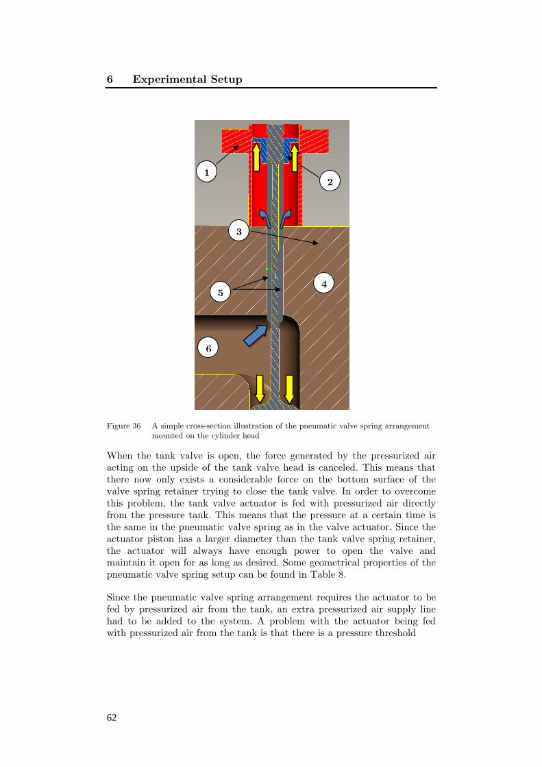
6 Experimental Setup
62
Figure 36 A simple cross-section illustration of the pneumatic valve spring arrangement mounted on the cylinder head
When the tank valve is open, the force generated by the pressurized air acting on the upside of the tank valve head is canceled. This means that there now only exists a considerable force on the bottom surface of the valve spring retainer trying to close the tank valve. In order to overcome this problem, the tank valve actuator is fed with pressurized air directly from the pressure tank. This means that the pressure at a certain time is the same in the pneumatic valve spring as in the valve actuator. Since the actuator piston has a larger diameter than the tank valve spring retainer, the actuator will always have enough power to open the valve and maintain it open for as long as desired. Some geometrical properties of the pneumatic valve spring setup can be found in Table 8.
Since the pneumatic valve spring arrangement requires the actuator to be fed by pressurized air from the tank, an extra pressurized air supply line had to be added to the system. A problem with the actuator being fed with pressurized air from the tank is that there is a pressure threshold
6
3
21
5 4
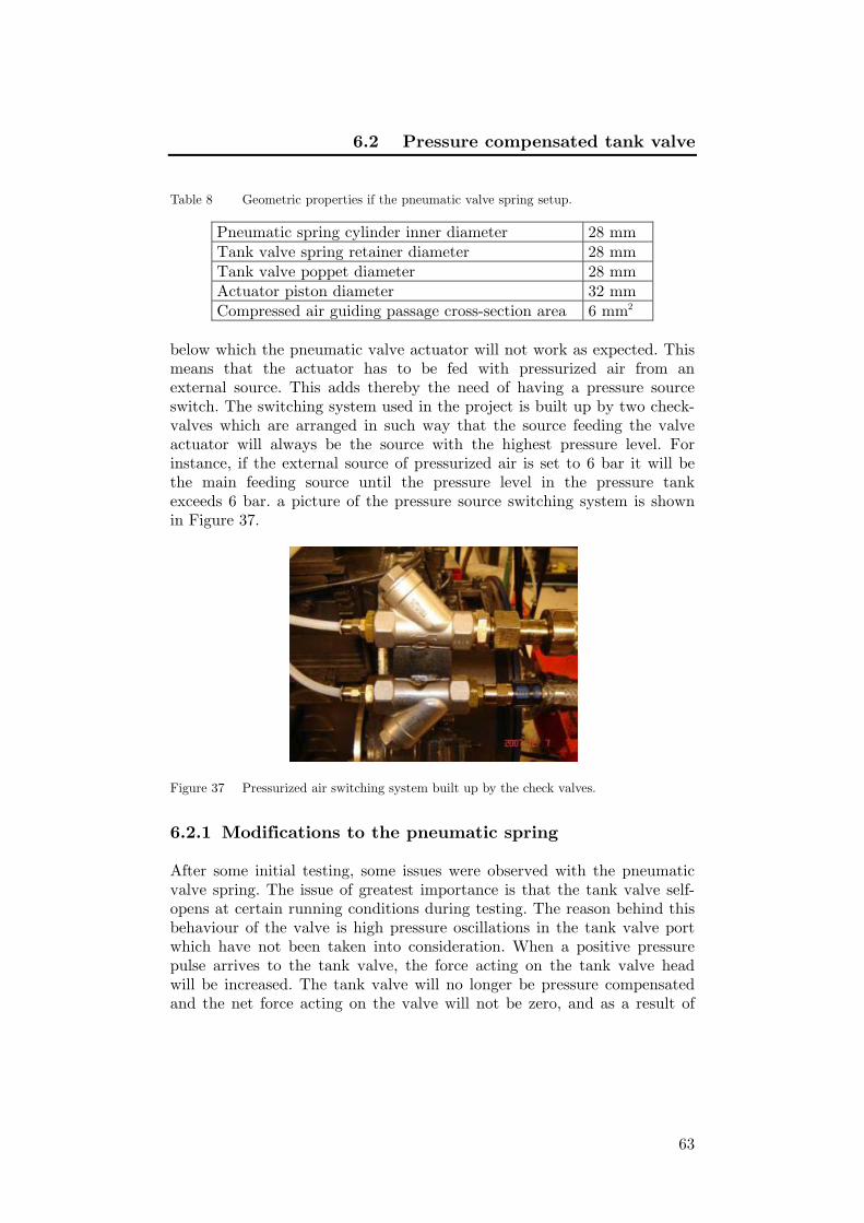
6.2 Pressure compensated tank valve
63
Table 8 Geometric properties if the pneumatic valve spring setup.
Pneumatic spring cylinder inner diameter 28 mm Tank valve spring retainer diameter 28 mm Tank valve poppet diameter 28 mm Actuator piston diameter 32 mm Compressed air guiding passage cross-section area 6 mm2
below which the pneumatic valve actuator will not work as expected. This means that the actuator has to be fed with pressurized air from an external source. This adds thereby the need of having a pressure source switch. The switching system used in the project is built up by two check-valves which are arranged in such way that the source feeding the valve actuator will always be the source with the highest pressure level. For instance, if the external source of pressurized air is set to 6 bar it will be the main feeding source until the pressure level in the pressure tank exceeds 6 bar. a picture of the pressure source switching system is shown in Figure 37.
Figure 37 Pressurized air switching system built up by the check valves.
6.2.1 Modifications to the pneumatic spring
After some initial testing, some issues were observed with the pneumatic valve spring. The issue of greatest importance is that the tank valve self-opens at certain running conditions during testing. The reason behind this behaviour of the valve is high pressure oscillations in the tank valve port which have not been taken into consideration. When a positive pressure pulse arrives to the tank valve, the force acting on the tank valve head will be increased. The tank valve will no longer be pressure compensated and the net force acting on the valve will not be zero, and as a result of

6 Experimental Setup
64
this the valve will self-open. In order to eliminate this problem a valve spring with 220 N preloading has been added to the tank valve, which means that there will always be a net force acting to keep the tank valve closed.
6.3 The Engine Control System
The engine control system consists of a purpose built program, a standard PC, Field Programmable Gate Array (FPGA) device card, A/D converters and sensors. The engine control program was built in LabVIEW, which is an entirely graphical programming language developed by National Instruments. The graphical user interface (GUI) is the link between the control program and the user, see Figure 38. From herer the user can for instance set desired valve lift, valve opening and closing, mode of operation, etc. The GUI also contains some important graphs such as cylinder pressure, tank pressure, valve lift and PV-diagram. The graphs are useful since they show the current status of the system in a very descriptive manner. The switch between modes of engine operation such as compressor mode and air-motor mode can easily be done by simply pushing the button for each engine mode respectively. The control program was used for both steady-state operation, where most of the parameters are set manually, and for continuously open- or closed-loop controlled operation where all the control parameters are read from
Figure 38 The GUI of the control program used in the engine control system.

6.3 The Engine Control System
65
predefined look-up tables or determined by the closed-loop controller.
The communication between the control program and the engine and its subsystem goes through an FPGA device of type NI PCI-7831R. The FPGA offers benefits such as precise timing, rapid decision making with loop rates up to 40 MHz and simultaneous execution of parallel tasks. All these benefits make the FPGA device a good tool for control of something so crucial as valve actuation and fuel injection. The NI PCI-7831R has 8 analog inputs, 8 analog outputs and 96 digital I/O.
For data acquisition a NI PCI-6259 multifunction data acquisition (DAQ) device was used. It has 32 analog inputs, 4 analog outputs and 48 digital I/O. With this system it is possible to simultaneously collect data in 32 channels at 1.25 MS/s.
There are several sensors measuring the engine running status. The cylinder pressure is measured by pressure transducers of type Kistler® 7061B. It is a piezoelectric pressure sensor which consists of a quartz crystal that is exposed to the gases through a diaphragm. When exposed to pressure, the crystal deforms and produces an electrical charge proportional to the pressure change in the cylinder. The electric charge is converted in a charge amplifier to an analog voltage signal. The charge amplifier used in the project summarized in present thesis is of type Kistler® 5011. The pressure transducer is water-cooled in order to resist the tough environment inside the combustion chamber.
The pressure transmitters used for measuring changes in tank pressure are piezoresistive transmitters of type 21 R from Keller. They are suitable for pressures from 1 to 100 bar and temperatures up to 100°C. One is positioned in the tank valve port, while the other is located at the inlet to the pressure tank.
To be able to measure the temperature of the compressed air right after the tank valve and in the pressure tank, temperature sensors from Pentronic of type K was utilized. They are mounted on the reconfigured intake port and on the pressure tank wall.

66
Chapter 7
7 Results
The pneumatic hybrid engine concept brings some new modes of engine operation in addition to the conventional ICE modes of operation. They include the compressor mode, air-motor mode and the air-power assist mode or supercharge mode. All these modes have been tested during the project described in this thesis and the results are presented in the following sections. In order to estimate the potential of a pneumatic hybrid vehicle, a vehicle model has been developed and its performance has been investigated through drive cycle simulations. These results will also be presented in following chapter.
7.1 Compressor Mode
The compressor mode is the mode during which the ICE is used as a 2-stoke compressor. There are mainly three different ways to operate the valves during compressor mode operation: with emphasis on maximum compressor mode efficiency, maximum compressor mode brake torque and lastly a combination of both.
7.1.1 Efficiency-Optimal Compressor Mode Operation with Theoretically Calculated Valve Timings
Efficiency-optimal compressor mode operation is achieved by keeping the compressor mode efficiency at a maximum. As mentioned above, this can be done by minimizing the energy consumed during the generation of compressed air. In Figure 39, the negative engine work as a function of TankVO during steady-state compressor mode operation at a constant tank pressure of 4 bar can be seen. It can clearly be noticed that there exists an operating point where the negative engine work is at a minimum, in this case at a TankVO of 70 CAD BTDC. This means that it takes less power to compress the inducted air at this point than at any other point on the curve at current tank pressure, which in turn means that the compressor mode operation is efficiency-optimal in this point.

7.1 Compressor Mode
67
This clearly indicates the importance of proper valve timing considering optimal compressor mode performance.
Figure 39 Negative engine work as a function of TankVO during steady-state compressor mode operation; tank pressure = 4 bar and engine speed = 600 rpm.
One way of achieving optimal compressor mode operation is to theoretically calculate the valve timings. As described in Section 3.2, during optimal compressor mode operation the tank valve should be controlled in such a way that the pressure inside the cylinder reaches the same pressure level as in the tank before the tank valve opens. In this way, a blowdown of pressurized air from the pressure tank or an excessive compression of the air trapped in the cylinder can be avoided.
The information above can be used for determining in which way the valve timings can be calculated. Since the tank pressure and the cylinder pressure can be measured they are to be considered as known. The maximum cylinder volume, i.e. the total cylinder volume when the piston is positioned at BDC, can be calculated with the help of engine specific geometrical data given in Table 4 and Table 7. The compression process in an ICE is a polytropic process since there exists a transfer of both heat and work between the system and its surroundings [104]. By assuming that air is an ideal gas, the following polytropic compression equation can be derived:
κ
12 1
2
Vp =pV
(7.1)
where p1 corresponds to the pressure at BDC and p2 is the pressure at any point in the cycle. V1 is the maximum volume in the cylinder and V2 is the cylinder volume at cylinder pressure p2 and κ (kappa) is the polytropic exponent. Setting p2 equal to the tank pressure the cylinder volume at the
050100150200400
450
500
550
600
650
700
750
TankVO [CAD BTDC]
Ne
ga
tive
En
gin
e W
ork
[J] Tank Pressure = 4 bar

7 Results
68
given pressure can be calculated. Then, by comparing the calculated V2 to a pre-calculated CAD-resolved volume trace, the crank-angle position at which the cylinder volume is equal to V2 can be established and this is the crank-angle position at which the tank valve should open. In this way it is possible to calculate an appropriate TankVO for all tank pressures. The same method can be used to establish correct TankVC and IVO.
The abovementioned method has the advantage that it is very simple and easy to implement in a control system. However, there are some drawbacks in using this method. One drawback is that the polytropic exponent, κ, depends on heat losses which mean that it will vary during the compression stroke and setting it to a constant value may introduce some errors in the determination of proper TankVO, see [105]. Another drawback with the proposed method is that certain dynamics of the system such as pressure wave propagation are neglected.
With the help of equation (7.1) the valve timings have be calculated and in Figure 40 the calculated TankVO can be seen.
Figure 40 TankVO calculated with the polytropic compression equation as a function of tank pressure.
Figure 41 shows the PV-diagram and tank pressure during one cycle of compressor mode operation. The calculated valve timings are all marked with dots together with a corresponding acronym in the figure. The PV-diagram bears a great resemblance with the ideal PV-diagram shown in Figure 6(b). The main difference occurs between TankVO and TankVC, where an overshoot in cylinder pressure can be noticed. The reason for this behavior, which occurs during real engine experiments, is flow restriction over the tank valve. A restriction in flow of compressed air across the tank valve will lead to an overshoot in cylinder pressure
5 10 15 20
20
30
40
50
60
70
80
Ta
nkV
O [C
AD
BT
DC
]
Tank Pressure [bar]

7.1 Compressor Mode
69
(a)
(b)
Figure 41 Cylinder pressure during compressor mode operation presented as a function of cylinder volume in a PV-diagram (a) and the corresponding tank pressure (b). The mean tank pressure is 6 bar and the engine speed is 600 rpm. (TVO – Tank Valve Opening, TVC – Tank Valve Closing)
since the engine generates compressed air at a higher rate than what can be discharged to the pressure tank. The restriction will also result in a pressure drop across the tank valve. This can clearly be seen by comparing Figure 41 (a) and (b) where the difference between maximum cylinder pressure and maximum tank pressure is about 2 bar. The overshoot in cylinder pressure also depends on when TankVO occurs. Retarding TankVO leads to an increase in overshoot since a late TankVO means that there will be less time to vent the cylinder from compressed air. This can clearly be seen in Figure 42 which illustrates the difference in cylinder pressure at two different TankVO.
Figure 42 PV-diagram of two engine cycles at a tank pressure of 4 and 12 bar, respectively, illustrating the difference in cylinder pressure overshoot between early and late TankVO.
0 0.5 1 1.5 2 2.50
2
4
6
8
10
12
Cylinder Volume [dm3]
Cyl
ind
er
Pre
ssu
re [b
ar]
TVC TVO
IVO IVC
Tank Pressure = 6 barTVO = 60 CAD BTDCTVC = 6 CAD ATDCIVO = 49 CAD ATDCIVC = 180 CAD ATDC
-150 -100 -50 0 50 100 1504
4.5
5
5.5
6
6.5
7
7.5
8
CAD [ATDC]
Ta
nk
Pre
ssu
re [b
ar]
TVO
TVC
IVO
IVC
0 0.5 1 1.5 2 2.50
2
4
6
8
10
12
14
16
Cylinder Volume [dm3]
Cyl
ind
er
Pre
ssu
re [b
ar]
TankP=4 barTVO=56 CAD BTDC
TankP=12 barTVO=33 CAD BTDC
P=3.2 bar
P=3.7 bar

7 Results
70
The restriction of the flow across the valve highly depends on the size of the tank valve, the tank pressure and the engine speed, which will be demonstrated in a Section 7.1.5.
(a)
(b)
Figure 43 (a) Negative IMEP and mean tank pressure during transient compressor mode operation as a function of engine cycle number, (b) Negative IMPE as a function of mean tank pressure. Engine speed = 600 rpm.
In Figure 43(a), an attempt to simulate a braking event can be seen. The event occurs over 800 engine revolutions, which is considerably longer compared to a typical braking event during real driving. However, this type of experiments serves as a way to estimate the performance of the compressor mode on an experimental single-cylinder engine. The valve timings are set according to the method described above. By investigating the IMEP curve it can be observed that the negative IMEP at first increases rapidly, and then starts to stagnate. One of the reasons for this behavior is the choice of valve timings. By comparing Figure 43, especially Figure 43(b), with Figure 40 it can be seen that the shape of the IMEP curve resembles the calculated TankVO curve in Figure 40 quite well. At low tank pressures, the difference in TankVO for a given pressure difference is much larger than at a high tank pressure for the same pressure difference, see Figure 44. A large change in TankVO will lead to a large change in IMEP while the opposite will only have a modest influence on IMEP.
Another reason for this behavior is the presence of the clearance volume in the cylinder, which is the volume in the cylinder when the piston reaches TDC. If the pressure in the cylinder is equal to the pressure in the tank, the compressed air contained in the clearance volume will never be transferred to the tank. During compressor mode operation, as the TankVO is retarded, the ratio of clearance volume to cylinder volume at TankVO will increase. At early TankVO, the aforementioned ratio will be small indicating that the influence of the clearance volume on IMEP is
0 200 400 600 8000
0.8
1.6
2.4
3.2
4
Ne
ga
tive
IME
P [b
ar]
Number of Engine Cycles [-]
0 200 400 600 8000
5
10
15
20
25
Ta
nk
Pre
ssu
re [b
ar]
Negative IMEPTank Pressure
5 10 15 200.5
1
1.5
2
2.5
3
Ne
ga
tive
IME
P [b
ar]
Tank Pressure [bar]

7.1 Compressor Mode
71
very limited. However, at late TankVO, this ratio will increase. During these situations the clearance volume will constitute a considerable part of the total volume at TankVO and therefore a change in TankVO will only result in a very small change in the total cylinder volume and thus the effect on IMEP will be limited.
Figure 44 Illustration showing that the difference in TankVO for a change in tank pressure of 1 bar is much larger at a low tank pressure compared to at a high tank pressure.
7.1.2 Efficiency-Optimal Compressor Mode Operation with Optimized Valve Timing
The abovementioned strategy to control the valves provides a simple solution and it is easy to implement in a control program. However, there are some disadvantages that may lead to inaccurate valve timings considering optimal compressor mode operation. In order to avoid these problems, proper valve timings can be determined through steady-state experiments. In Figure 39, it was shown that at a given pressure there exists a TankVO for which the energy consumed during compressor mode is at a minimum and thus maximum efficiency can be expected in this point.
As stated above, a TankVO sweep can serve as a method to find optimal TankVO at a given tank pressure during steady-state compressor mode operation. In Figure 45(a), TankVO sweeps at 4 different steady-state tank pressures can be seen. All sweeps show similar trends with a minimum in negative IMEP and thus a minimum in negative brake energy at some point on the curve. If however higher brake power is needed, the efficiency has to be sacrificed. By advancing TankVO from the optimal point the IMEP will increase. The reason is that with an early TankVO, the pressure in the cylinder is lower compared to the pressure in the tank, and therefore there will be a blowdown of compressed air from
-100 -80 -60 -40 -20
2
4
6
8
10
12
14
16
18
20
TankVO [ATDC]
Ta
nk
Pre
ssu
re [b
ar]
p=1 bar
p=1 bar

7 Results
72
the tank into the cylinder. The blowdown of compressed air contributes with negative work since the piston has to work against a higher pressure in the cylinder.
(a)
(b)Figure 45 Steady-state optimization of the compressor mode at an engine speed of 600
rpm; (a) Negative IMEP as a function of TankVO for different tank pressures; (b) Optimal TankVO and corresponding negative IMEP as a function of tank pressure.
In Figure 45(b), the most optimal TankVO and corresponding negative IMEP together with the theoretically calculated TankVO have been plotted. There are mainly two reasons why negative IMEP decreases after a tank pressure of about 14 bar. One reason is that during the TankVO sweep the TankVC is kept constant. Ideally the TankVC should occur during the expansion stroke at the moment when the pressure in the cylinder equals the pressure in the tank. At tank pressures above 14 bar in Figure 45(b) the IMEP decreases since the tank valve closes too late which means that the pressure in the cylinder will decrease below the tank pressure, and a blowdown of pressurized air will occur. The blowdown of compressed air will in this case contribute with positive work and thus IMEP will decrease. The other reason for the decrease in IMEP is system dynamics in the form of pressure wave propagation through the system. A more in-depth look at both these phenomena will be presented later in a following section.
Another thing that can be observed in Figure 45(b) is that there is a considerable difference between theoretically calculated valve timings and experimentally optimized valve timings. At some points the difference in TankVO between the two cases is as high as 10 CAD which clearly indicates the problem with the theoretical approach. The occurrence of this behavior can mainly be attributed to delays associated with the VVA system and pressure wave propagation.
0501001502002
3
4
5
6
7
TankVO [CAD BTDC]
Ne
ga
tive
IME
P [b
ar]
4 bar10 bar15 bar21 bar
3 6 9 12 15 18 21
20
35
50
65
80T
an
kVO
[CA
D B
TD
C]
Tank Pressure [bar]
3 6 9 12 15 18 211.5
2
2.5
3
3.5
Ne
ga
tive
IME
P [b
ar]
Optimized TankVOTheoretical TankVONegative IMEP

7.1 Compressor Mode
73
(a)
(b)
Figure 46 Comparison of transient compressor mode operation with theoretical and optimized valve timings: (a) Negative IMEP as a function of engine cycle number; (b) COP as a function of engine cycle number.
mode operation can be seen. Initially, negative IMEP for the theoretical case is similar to the negative IMEP for the optimized case. However, after approximately 300 engine cycles, negative IMEP for the optimized case remains reasonably constant while negative IMEP for the theoretical case continuous to increase throughout the experiment. Figure 46(b) indicates that there is a very small difference in COP between the two cases. The total COP, which is the accumulated COP during the entire experiment, for the optimized case is improved by merely 0.014 units compared to the theoretical case, which corresponds to an improvement of about 1.7%. The conclusion from these results is that even though there was a considerable difference between the two cases regarding valve timings and IMEP, the efficiency is almost the same which indicates that the theoretical approach serves as a good alternative to the more laborious optimization approach. In other words, there is not much to gain by experimentally optimizing the valve timings for the compressor mode. In Figure 46(a) it can also be seen that the final tank pressure is 0.2 bar lower for the optimized case compared to the theoretical case even though the latter case showed a somewhat lower efficiency. This behavior implies that there are some underlying phenomena affecting the compressor mode performance and motivates a parametric study of the compressor mode which can be found in Section 7.1.5.
7.1.3 The Influence of Valve Head Diameter on Compressor Mode Performance
The overshoot in cylinder pressure during compressor mode operation illustrated in Figure 42 raises the question whether this overshoot can be decreased and how a decrease will affect the performance of the
0 200 400 600 8000
0.5
1
1.5
2
2.5
3
3.5
Number of Engine Cycles
Ne
ga
tive
IME
P [b
ar]
Theoretical Valve TimingFinal TankP = 21.2 barOptimized Valve TimingFinal TankP = 21.0 bar
0 200 400 600 8000
0.5
1
1.5
2
2.5
Number of Engine Cycles
CO
P C
om
pre
sso
r M
od
e [-
]
Theroretical Valve TimingCOP
tot = 0.814
Optimized Valve TimingCOP
tot = 0.828

7 Results
74
compressor mode. In an attempt to find an answer to this question, the tank valve head diameter was identified as a parameter directly affecting the flow of compressed air from the cylinder and into the tank. The results in previous subsections where obtained with the experimental setup described in Paper I where the tank valve head diameter was 16 mm. By increasing the diameter to 28 mm, the flow was increased more than three times. As mentioned in Section 6.2, in order to ensure proper tank valve operation at high in-cylinder pressures, the larger tank valve was combined with an in-house developed pneumatic valve spring which makes the tank valve pressure compensated.
Figure 47 Negative IMEP during compressor mode operation for two different tank valve configurations as a function of TankVO at various tank pressures and an engine speed of 600 rpm.
In Figure 47 the results from TankVO sweeps for two different tank valve configurations at three different tank pressures can be seen. At a tank pressure of 4 bar there is a considerable difference in IMEP between the two tank valve configurations. This is as expected, since a larger tank valve head diameter allows a higher flow of compressed air across the valve and into the tank which results in a lower overshoot in cylinder pressure. However, at 10 and 15 bar there is hardly any difference between minimum negative IMEP for the large tank valve compared to the small tank valve. The only difference is that the optimal TankVO for the large tank valve is advanced a number of CAD compared to TankVO for the small tank valve. A reason for this behaviour is that there is some pressure losses in the pressurized air supply line between the tank and the pneumatic valve actuator, which means that the pressurized air fed to the valve actuator at a certain time is not the same as the mean tank pressure at the corresponding time and therefore the ability to open the tank valve at optimal timing is lost and has to be advanced. An advance in TankVO compared to optimal timing means that there will be a blowdown of pressurized air into the cylinder and thus negative IMEP will increase.
204060801001201
2
3
4
5
6
7
TankVO [CAD BTDC]
Ne
ga
tive
IME
P [b
ar]
4 bar,=1610 bar,=1615 bar,=164 bar,=2810 bar,=2815 bar,=28

7.1 Compressor Mode
75
The reason why negative IMEP for the large tank valve is considerably lower than for the small tank valve at 4 bar of tank pressure is that at this tank pressure level, the actuator is fed with 6 bar of compressed air from an external source. This means that, at this point there is a surplus of 2 bar feeding the valve actuator and thus optimal TankVO timing can be achieved.
(a) (b) Figure 48 Optimized TankVO (a) and corresponding negative IMEP (b) as a function of
tank pressure for two different tank valve configurations.
Figure 48 shows how optimal TankVO (a) and corresponding negative IMEP (b) varies with tank pressure for two different tank valve configurations. In Figure 48(a) it can be seen that the optimal TankVO for the large tank valve occurs considerably earlier compared to the optimal TankVO for the small tank valve. The reason for this behavior can once again be explained as inadequate amount of pressurized air supplied to the tank valve actuator and therefore the valve timing has to be advanced a number of CAD away from the real optimum, which contributes to a higher negative IMEP.
Figure 49 shows PV-diagrams of the cylinder pressure for the two valve configurations at tank pressures of 4 and 12 bar, respectively. The PV-diagram for the large tank valve setup in Figure 49(a), bear a great resemblance with an ideal compressor mode PV-diagram. The Cylinder pressure is almost constant during the pressure tank charging between cylinder volume 1 and 0.2 dm3. The overshoot is about 0.5 bar which is considerably lower than the overshoot of 3.5 bar for the small tank valve. Figure 49(b) shows that at a tank pressure of 12 bar the overshoot increases by 1 bar for the large valve, while the corresponding increase for the small tank valve is about 0.5 bar. The reason why the increase in overshoot is larger for the large valve is that due to reasons stated above, the TankVO has to be advanced in comparison to optimal TankVO. This can clearly be seen in Figure 49(b), where the cylinder pressure for the
3 6 9 12 15 18 21
20
35
50
65
80
Tank Pressure [bar]
Ta
nkV
O [C
AD
BT
DC
]
= 16 = 28
3 6 9 12 15 18 210.5
1
1.5
2
2.5
3
3.5
Tank Pressure [bar]
Ne
ga
tive
IME
P [b
ar]
= 16 = 28
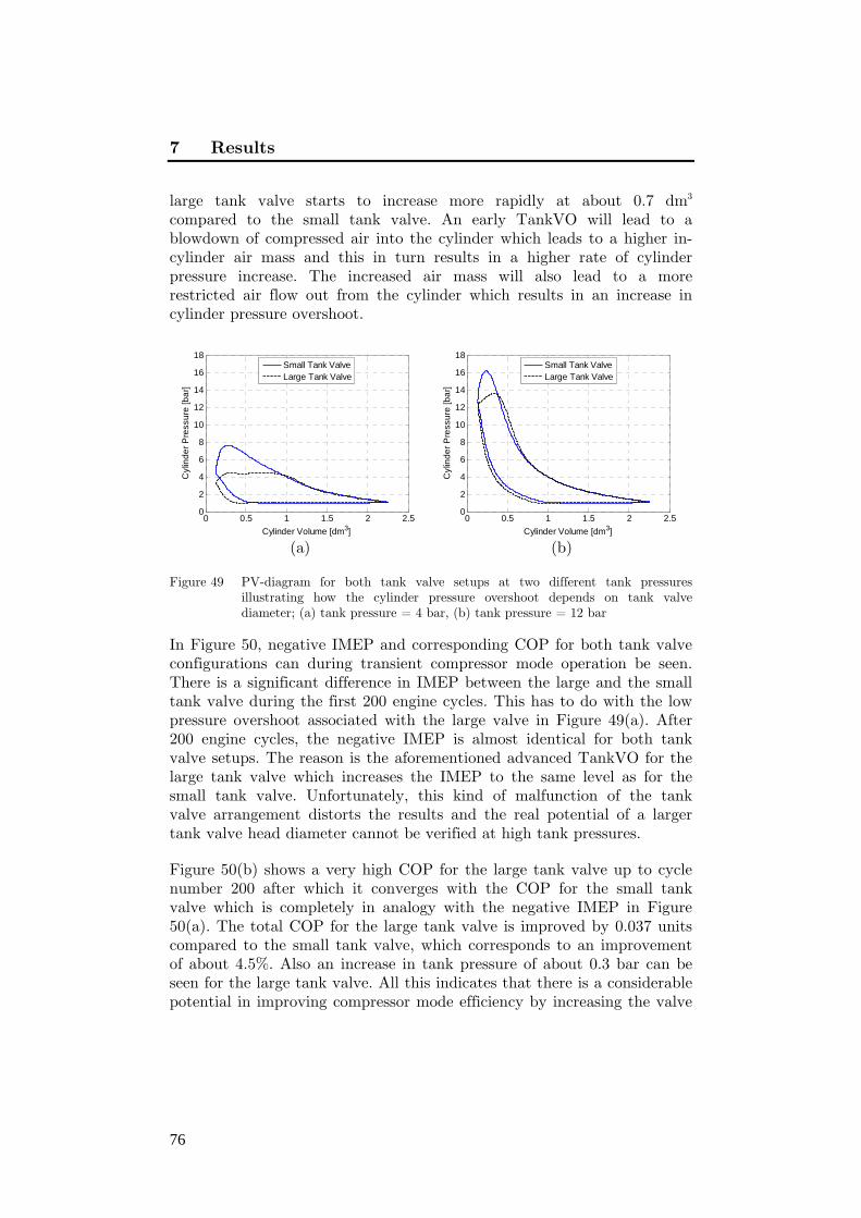
7 Results
76
large tank valve starts to increase more rapidly at about 0.7 dm3 compared to the small tank valve. An early TankVO will lead to a blowdown of compressed air into the cylinder which leads to a higher in-cylinder air mass and this in turn results in a higher rate of cylinder pressure increase. The increased air mass will also lead to a more restricted air flow out from the cylinder which results in an increase in cylinder pressure overshoot.
(a) (b)
Figure 49 PV-diagram for both tank valve setups at two different tank pressures illustrating how the cylinder pressure overshoot depends on tank valve diameter; (a) tank pressure = 4 bar, (b) tank pressure = 12 bar
In Figure 50, negative IMEP and corresponding COP for both tank valve configurations can during transient compressor mode operation be seen. There is a significant difference in IMEP between the large and the small tank valve during the first 200 engine cycles. This has to do with the low pressure overshoot associated with the large valve in Figure 49(a). After 200 engine cycles, the negative IMEP is almost identical for both tank valve setups. The reason is the aforementioned advanced TankVO for the large tank valve which increases the IMEP to the same level as for the small tank valve. Unfortunately, this kind of malfunction of the tank valve arrangement distorts the results and the real potential of a larger tank valve head diameter cannot be verified at high tank pressures.
Figure 50(b) shows a very high COP for the large tank valve up to cycle number 200 after which it converges with the COP for the small tank valve which is completely in analogy with the negative IMEP in Figure 50(a). The total COP for the large tank valve is improved by 0.037 units compared to the small tank valve, which corresponds to an improvement of about 4.5%. Also an increase in tank pressure of about 0.3 bar can be seen for the large tank valve. All this indicates that there is a considerable potential in improving compressor mode efficiency by increasing the valve
0 0.5 1 1.5 2 2.50
2
4
6
8
10
12
14
16
18
Cylinder Volume [dm3]
Cyl
ind
er
Pre
ssu
re [b
ar]
Small Tank ValveLarge Tank Valve
0 0.5 1 1.5 2 2.50
2
4
6
8
10
12
14
16
18
Cylinder Volume [dm3]
Cyl
ind
er
Pre
ssu
re [b
ar]
Small Tank ValveLarge Tank Valve

7.1 Compressor Mode
77
head diameter even though only a small part of the complete transient experiment is executed with fully functional tank valve operation.
(a) (b) Figure 50 Comparison of transient compressor mode operation for two different tank
valve configurations: (a) Negative IMEP and tank pressure as a function of engine cycle number; (b) COP as a function of engine cycle number.
Figure 13 is an attempt to illustrate what happens to the operational capability of the tank valve during the transient experiment shown in Figure 50. In Figure 51(a), the difference between maximum cylinder pressure and maximum tank pressure is displayed. For the small tank valve setup the pressure difference is initially above 1.5 bar, but as the transient experiment continues the pressure difference decreases and ends at about 0.5 bar. This can be explained by the fact that at low tank pressures the TankVO occurs early during the compression stroke and consequently the charging of compressed air into the tank occurs over a considerable part of the compression stroke. In other words, the air contained in the cylinder after TankVO will be exposed to a compressing force during a substantial part of the compression stroke, thus making it achieve a high peak pressure. At high tank pressures, the TankVO occurs late during the compression stroke which results in the fact that only a small part of the compression stroke occurs after TankVO. This means that the air contained in the cylinder after TankVO will be exposed to a compressing force during a very limited time and thus the overshoot in tank pressure will be small compared to early TankVO.
The pressure difference for the large tank valve, on the other hand, starts at about 0 bar and works its way up to about 1.3 bar at the end of the transient experiment. This can be explained with the help of Figure 51(b). At the beginning of the transient experiment, the tank valve achieves its maximum lift height of 7 mm and the pressure difference is therefore held at a minimum. However, as the transient experiment proceeds, the pressure difference increases, mainly due to the inability of the valve
0 200 400 600 8000
1
2
3
4
Ma
ss F
low
[g/c
ycle
]
Number of Engine Cycles [-]
0 200 400 600 8000
5
10
15
20
25
Ta
nk
Pre
ssu
re [b
ar]
0 200 400 600 8000
5
10
15
20
25=16 mm=28 mm
0 200 400 600 8000
1
2
3
4
5
6
Number of Engine Cycles
CO
P C
om
pre
sso
r M
od
e [-
]
=16 mm, COPtot
= 0.828
=28 mm, COPtot
= 0.865
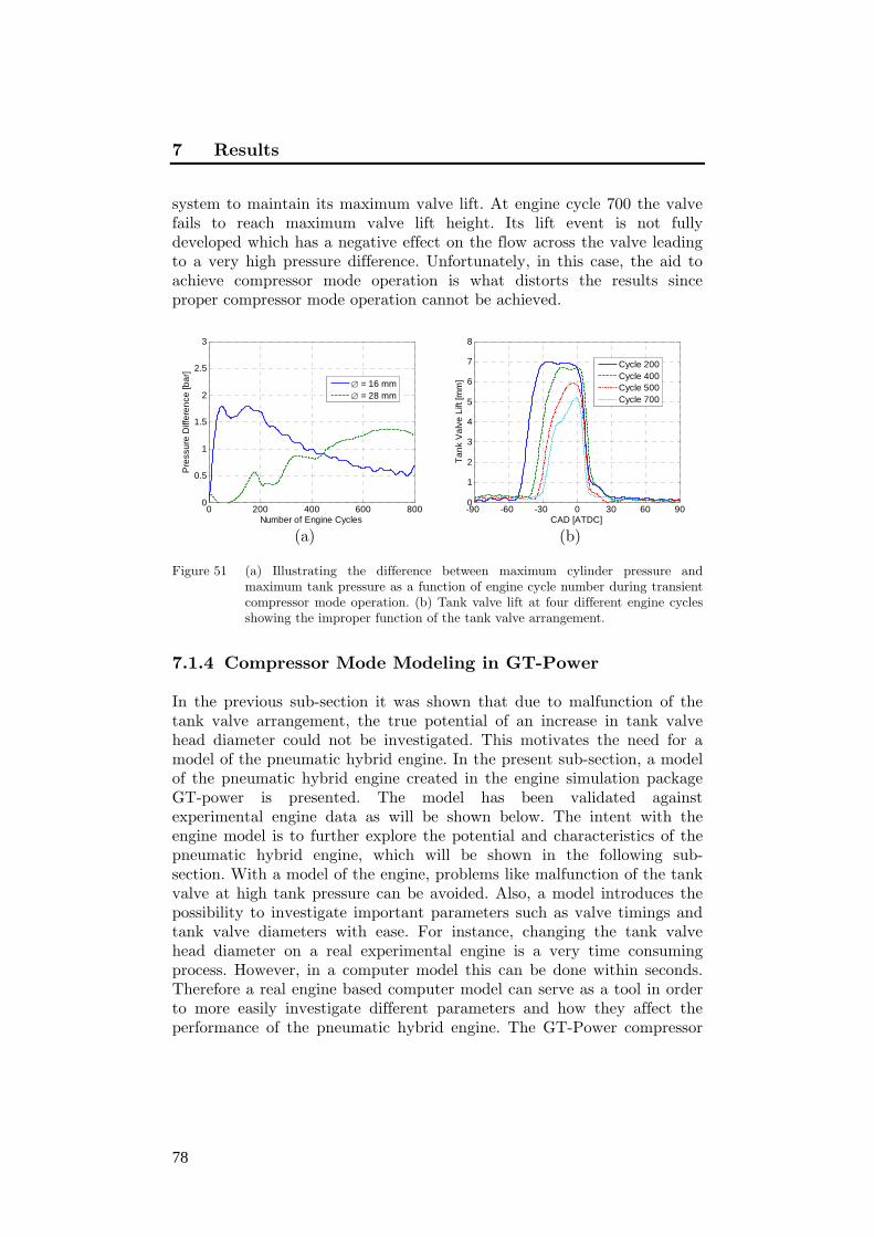
7 Results
78
system to maintain its maximum valve lift. At engine cycle 700 the valve fails to reach maximum valve lift height. Its lift event is not fully developed which has a negative effect on the flow across the valve leading to a very high pressure difference. Unfortunately, in this case, the aid to achieve compressor mode operation is what distorts the results since proper compressor mode operation cannot be achieved.
(a) (b)
Figure 51 (a) Illustrating the difference between maximum cylinder pressure and maximum tank pressure as a function of engine cycle number during transient compressor mode operation. (b) Tank valve lift at four different engine cycles showing the improper function of the tank valve arrangement.
7.1.4 Compressor Mode Modeling in GT-Power
In the previous sub-section it was shown that due to malfunction of the tank valve arrangement, the true potential of an increase in tank valve head diameter could not be investigated. This motivates the need for a model of the pneumatic hybrid engine. In the present sub-section, a model of the pneumatic hybrid engine created in the engine simulation package GT-power is presented. The model has been validated against experimental engine data as will be shown below. The intent with the engine model is to further explore the potential and characteristics of the pneumatic hybrid engine, which will be shown in the following sub-section. With a model of the engine, problems like malfunction of the tank valve at high tank pressure can be avoided. Also, a model introduces the possibility to investigate important parameters such as valve timings and tank valve diameters with ease. For instance, changing the tank valve head diameter on a real experimental engine is a very time consuming process. However, in a computer model this can be done within seconds. Therefore a real engine based computer model can serve as a tool in order to more easily investigate different parameters and how they affect the performance of the pneumatic hybrid engine. The GT-Power compressor
0 200 400 600 8000
0.5
1
1.5
2
2.5
3
Number of Engine Cycles
Pre
ssu
re D
iffe
ren
ce [b
ar]
= 16 mm = 28 mm
-90 -60 -30 0 30 60 900
1
2
3
4
5
6
7
8
CAD [ATDC]
Ta
nk
Va
lve
Lift
[mm
]
Cycle 200Cycle 400Cycle 500Cycle 700

7.1 Compressor Mode
79
mode model was validated against measured data from different steady-state operating points. In order to estimate the accuracy of the model, the relative error between measured data and model data had to be calculated. The relative error can be described by the following equation:
0x-xδx=x
(7.2)
where x is the model data and x0 is the measured data. Below, only results at 600 rpm are shown since the results at 900 rpm show a very similar trend making them redundant here. The results obtained at 900 rpm can be found in [106].
Figure 52 shows how measured and simulated negative IMEP and corresponding relative error varies with increasing tank pressure. The simulated curve reproduces very closely the shape of the measured data and the relative error is generally within 1%.
Figure 52 Negative IMEP and corresponding relative error as a function of tank pressure during measured and simulated steady-state compressor mode operation at an engine speed of 600 rpm
The maximum cylinder pressure as a function of tank pressure is illustrated in Figure 53(a). The simulated data shows a good agreement with measured data. The results are within a 5% agreement which indicates that the conditions inside the cylinder are recreated quite well.
In Figure 53(b), the maximum tank pressure at different mean tank pressure can be seen. The agreement between simulated and measured data is in this case not as good as in previous figures. The relative error exceeds 5% at almost all operating points. The fact that the relative error is almost constant indicates that the error might arise due to the type of pressure sensor used to measure the port pressure. The sensor in question
1
1.5
2
2.5
3
Ne
ga
tive
IME
P [b
ar]
MeasGTP
0 5 10 15 20 25 300123
Tank Pressure [bar]
x [%
]

7 Results
80
is a piezoresistive transducer and according to tests done by Tsung et al. [107] the response rate of such transducers are one fourth of the response rate of piezoelectric transducers usually used for in-cylinder pressure measurement. This means that the pressure signal achieved with the piezoresistive transducer is damped and therefore deviates from what would be achieved with a piezoelectric transducer.
(a) (b)Figure 53 Maximum cylinder pressure (a) and maximum tank pressure (b) together with
corresponding relative error as a function of tank pressure during measured and simulated steady-state compressor mode operation at an engine speed 0f 600 rpm.
So far the model has shown satisfactory agreement with steady-state measured data. However, to fully explore the accuracy of the model it needs to be tested during transient engine operation as well. In Figure 54, negative IMEP during transient compressor mode operation is presented. The agreement between simulated and measured data is reasonably good with a relative error mainly within 5%. If these results from transient operation are compared with those obtained during steady-state simulations, it can be noticed that transient operation leads to a higher relative error. There might be various possible reasons for such behavior. The most probable is that transient gas dynamics differs from stationary conditions and therefore some deviations between the results have to be expected.
Figure 55(a) shows maximum cylinder pressure data during transient compressor mode operation. In Figure 53(a) it could be seen that during steady-state compressor mode operation, the model over-predicts the maximum cylinder pressure at almost all operating points. However, during transient compressor mode operation the model under-predicts the cylinder pressure during almost the entire transient experiment. Once again this behavior can be attributed to the transient gas dynamics.
0
5
10
15
20
25
Ma
x C
ylin
de
r P
ress
ure
[ba
r]
MeasGTP
0 5 10 15 20 25 300
5
Tank Pressure [bar]
x [%
]
0
5
10
15
20
25
Ma
x T
an
k P
ress
ure
[ba
r]
MeasGTP
0 5 10 15 20 25 300
5
10
Tank Pressure [bar]
x [%
]

7.1 Compressor Mode
81
Mean tank pressure shows a good agreement between measured and simulated data during transient compressor mode operation, as can be seen in Figure 55(b). The predicted data lies within ±5% of the measured
Figure 54 Negative IMEP and corresponding relative error as a function of engine cycle number during measured and simulated transient compressor mode operation at an engine speed of 600 rpm.
(a) (b)
Figure 55 Maximum cylinder pressure (a) and mean tank pressure (b) together with corresponding relative error as a function of engine cycle number during measured and simulated transient compressor mode operation at an engine speed of 600 rpm.
data. A comparison between Figure 55(b) and Figure 53(b) indicates that simulated mean tank pressure shows a better agreement with measured data than simulated maximum tank pressure. The reason is probably that, due to the nature of the piezoresistive pressure sensor, the signal is somewhat averaged. Therefore, measured maximum tank pressure will differ from real maximum tank pressure. However, since the signal is already averaged, mean tank pressure will show a better agreement with predicted data.
0
1
2
3
4
Ne
ga
tive
IME
P [b
ar]
MeasGTP
0 200 400 600 800-5515
Number of Engine Cycles
x [%
]
0
5
10
15
20
25
30
Ma
x C
ylin
de
r P
ress
ure
[ba
r]
MeasGTP
0 200 400 600 800-15015
Number of Engine Cycles
x[%
] 0
5
10
15
20
25
Me
an
Ta
nk
Pre
ssu
re [b
ar]
MeasGTP
0 200 400 600 800-808
Number of Engine Cycles
x [%
]

7 Results
82
The conclusion from the results in the present sub-section is that a model that shows satisfying agreement with measured data has been realized. However, more modifications and tuning of the model should be done in the future in order to increase the accuracy to a maximum.
7.1.5 Parametric Study of Compressor Mode Performance
The main goal during compressor mode is always to, at any given situation, maximize the charging of the pressure tank. In Section 7.1.2 it could be noticed that even though the valve timings were optimized with regards to maximum compressor mode efficiency, the tank pressure decreased compared to the less accurate theoretical approach. This leads to the conclusion that there are some underlying phenomena affecting the performance of the compressor mode. The purpose of this subsection is to investigate different parameters in order to understand their influence on the compressor mode performance. The relevant parameters which will be investigated are the tank valve diameter, tank valve opening and closing, and inlet valve opening. There are some additional parameters influencing the performance of the compressor mode, but their influences are small compared to the ones mentioned above and they are therefore omitted here.
Most of the results in this sub-section are obtained from the model described in the previous sub-section since a parametric study on a experimental engine would be too time consuming and measurements such as mass flow across the valves were not possible to obtain in the experimental setups used in the project described in this thesis.
Tank Valve Diameter
Adequate tank valve head diameter was identified as an important factor for maximum compressor mode efficiency. Unfortunately, the experimental results regarding change in valve diameter and its effect on compressor mode performance were somewhat misleading due to failure in the tank valve arrangement. However, with the help of the model described in previous sub-section, the true effect of tank valve head diameter on compressor performance can be investigated.
The size of the valve diameter is an important factor since it affects the mass flow across the valve. The mass is a direct measure of the compressor mode performance. The higher the mass flow, the higher the energy transfer to the tank. Figure 56 shows PV-diagrams of compressor mode operation at a tank pressure of 10 bar for three valve head diameters at 600 and 1500 rpm, respectively. It can clearly be seen how

7.1 Compressor Mode
83
the overshoot in cylinder pressure decreases with tank valve diameter. Also the engine speed plays an important role here. At an engine speed of 600 rpm, the overshoot in cylinder pressure with the 16 mm tank valve is larger compared to the other valve configurations but still at a reasonable level. However, at an engine speed of 1500 rpm, the cylinder pressure overshoots by more than 10 bar compared to the cylinder pressure for the 32 mm tank valve, which implies that the flow of compressed air across the tank valve is extremely restricted. In Table 9, a summary of relevant data associated with the PV-diagrams in Figure 56 can be seen. At an engine speed of 600 rpm negative IMEP decreases with valve diameter while the mass flow remains almost constant. At 1500 rpm the opposite behaviour can be detected, ie the IMEP remains constant while mass flow increases with valve diameter. This phenomenon can be explained with the help of Figure 56. In Figure 56(a), the only difference between the
(a) (b)
Figure 56 PV-diagram during steady-state compressor mode operation for various tank valve diameters at a tank pressure of 10 bar; (a) 600 rpm, (b) 1500 rpm.
different valve setups is the amount of overshoot in cylinder pressure. Since IMEP is defined as the area of the enclosed loop, an increase in IMEP when the overshoot increases can be expected. However, the cylinder pressure at TDC, i.e. when the cylinder volume is at a minimum, is about the same for all three cases which means that the mass of compressed air trapped in the cylinder at TDC is the same. This in turn means that the mass flow across the valve is the same for all three setups, as can be seen in Table 9. In Figure 56(b), there is a clear difference between the three setups regarding cylinder pressure overshoot and cylinder pressure at TDC. The cylinder pressure at TDC for the 16 mm setup is about 5 bar higher compared to the other setups. This indicates that the amount of compressed air left in the cylinder after TDC is higher for the 16 mm setup compared to the other two setups and consequently a lower mass flow can be expected, as can be seen in Table 9. A side-effect
0 0.5 1 1.5 2 2.50
5
10
15
20
25
Cylinder Volume [dm3]
Cyl
ind
er
Pre
ssu
re [b
ar]
=16 mm=24 mm=32 mm
0 0.5 1 1.5 2 2.50
5
10
15
20
25
Cylinder Volume [dm3]
Cyl
ind
er
Pre
ssu
re [b
ar]
=16 mm=24 mm=32 mm

7 Results
84
that arises from this behaviour is that, during the expansion stroke this excessive amount of compressed air trapped in the cylinder will contribute with positive work which in turn decreases the total negative work of the complete cycle. This result in an IMEP that is almost at the same level for all setups even though the cylinder pressure overshoot is considerably larger for the 16 mm setup compared to the other setups.
Table 9 Illustrating the influence of tank valve diameter and engine speed on negative IMEP and mass flow during steady-state compressor mode operation; tank pressure = 10 bar.
Engine speed [rpm] ø [mm]
IMEP [bar]
Mflow [g/cycle]
600 16 2.71 1.52 24 2.53 1.52 32 2.49 1.51
1500 16 3.03 1.24 24 3.13 1.51 32 3.00 1.51
In Figure 57 and Figure 58, the results from transient compressor mode operation for the two valve configurations at 600 and 1200 rpm, respectively, are shown. The results at 600 rpm are in analogy with what has previously been shown for steady-state operation. In Figure 56(a), a considerable difference in IMEP for the two setups can be seen. As previously established, the occurrence of this difference at 600 rpm is due to the difference in cylinder pressure overshoot. Figure 57(a) shows that there is hardly any difference in either mass flow or tank pressure during transient compressor mode operation at 600 rpm, which also correlates well with what has been established above. The total COP for the 16 mm and 32 mm setup at 600 rpm are 0.767 and 0.823, respectively. This corresponds to an increase in COP by 7.3% when switching from 16 mm

7.1 Compressor Mode
85
(a) (b) Figure 57 Transient compressor mode operation for two different valve setups at an
engine speed of 600 rpm; (a) Negative IMEP, (b) Mass flow and tank pressure.
(a) (b)
Figure 58 Transient compressor mode operation for two different valve setups at an engine speed of 1500 rpm; (a) Negative IMEP, (b) Mass flow and tank pressure.
to 32 mm in tank valve diameter. By definition, COP is the ratio between the energy stored in the tank and the energy consumed by the engine in order to generate the compressed air. In this case, the improvement in COP comes mainly from the decrease in IMEP since the tank pressure is similar for both valve setups.
At 1500 rpm, the results are comparable to what has been shown for steady state operation earlier. Figure 58 displays that there is a great similarity in IMEP while both mass flow and tank pressure differ considerably between the two tank valve setups, which agrees well with what has been established above for the steady-state operation at 1500 rpm. The total COP for the 16 mm and the 32 mm setups at 1500 rpm are 0.648 and 0.753, respectively. This corresponds to an increase in COP by 16.2% when switching from 16 mm to 32 mm tank valve diameter.
0 200 400 600 8000.5
1
1.5
2
2.5
3
3.5
Number of Engine Cycles [-]
Ne
ga
tive
IME
P [b
ar]
=16 mm,COPtot
=0.767
=32 mm,COPtot
=0.823
0 200 400 600 8000.2
1
1.8
2.6
3.4
Ma
ss F
low
[g/c
ycle
]
Number of Engine Cycles [-]
0 200 400 600 8000
6
12
18
24
Ta
nk
Pre
ssu
re [b
ar]
0 200 400 600 8000
6
12
18
24
=16 mm=32 mm
0 200 400 600 8000.5
1
1.5
2
2.5
3
3.5
Number of Engine Cycles [-]
Ne
ga
tive
IME
P [b
ar]
=16 mm,COPtot
=0.648
=32 mm,COPtot
=0.753
0 200 400 600 8000.2
1
1.8
2.6
3.4
Ma
ss F
low
[g/c
ycle
]
Number of Engine Cycles [-]
0 200 400 600 8000
6
12
18
24
Ta
nk
Pre
ssu
re [b
ar]
0 200 400 600 8000
6
12
18
24
=16 mm=32 mm
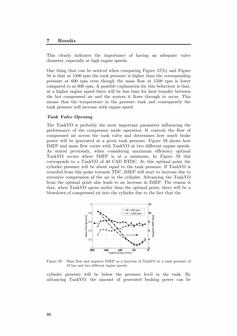
7 Results
86
This clearly indicates the importance of having an adequate valve diameter, especially at high engine speeds.
One thing that can be noticed when comparing Figure 57(b) and Figure 58 is that at 1500 rpm the tank pressure is higher than the corresponding pressure at 600 rpm even though the mass flow at 1500 rpm is lower compared to at 600 rpm. A possible explanation for this behaviour is that, at a higher engine speed there will be less time for heat transfer between the hot compressed air and the system it flows through to occur. This means that the temperature in the pressure tank and consequently the tank pressure will increase with engine speed.
Tank Valve Opening
The TankVO is probably the most important parameter influencing the performance of the compressor mode operation. It controls the flow of compressed air across the tank valve and determines how much brake power will be generated at a given tank pressure. Figure 59 shows how IMEP and mass flow varies with TankVO at two different engine speeds. As stated previously, when considering maximum efficiency optimal TankVO occurs where IMEP is at a minimum. In Figure 59 this corresponds to a TankVO of 40 CAD BTDC. At this optimal point the cylinder pressure will be about equal to the tank pressure. If TankVO is retarded from this point towards TDC, IMEP will start to increase due to excessive compression of the air in the cylinder. Advancing the TankVO from the optimal point also leads to an increase in IMEP. The reason is that, when TankVO opens earlier than the optimal point, there will be a blowdown of compressed air into the cylinder due to the fact that the
Figure 59 Mass flow and negative IMEP as a function of TankVO at a tank pressure of 10 bar and two different engine speeds.
cylinder pressure will be below the pressure level in the tank. By advancing TankVO, the amount of generated braking power can be
-200 -150 -100 -50 01
1.2
1.4
1.6
1.8
2
Ma
ss F
low
[g/c
ycle
]
TankVO [CAD ATDC]
-200 -150 -100 -50 02
4
6
8
10
12
Ne
ga
tive
IME
P [b
ar]
-200 -150 -100 -50 02
4
6
8
10
12
600 rpm1200 rpm
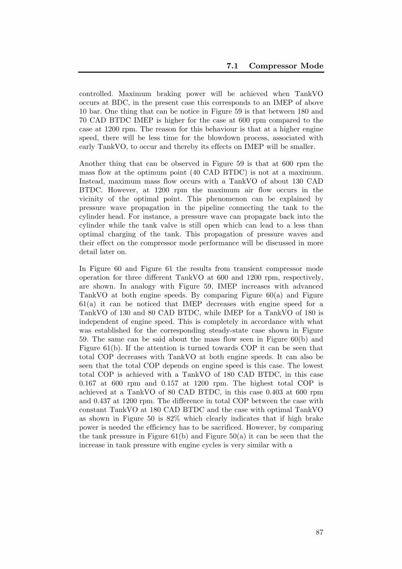
7.1 Compressor Mode
87
controlled. Maximum braking power will be achieved when TankVO occurs at BDC, in the present case this corresponds to an IMEP of above 10 bar. One thing that can be notice in Figure 59 is that between 180 and 70 CAD BTDC IMEP is higher for the case at 600 rpm compared to the case at 1200 rpm. The reason for this behaviour is that at a higher engine speed, there will be less time for the blowdown process, associated with early TankVO, to occur and thereby its effects on IMEP will be smaller.
Another thing that can be observed in Figure 59 is that at 600 rpm the mass flow at the optimum point (40 CAD BTDC) is not at a maximum. Instead, maximum mass flow occurs with a TankVO of about 130 CAD BTDC. However, at 1200 rpm the maximum air flow occurs in the vicinity of the optimal point. This phenomenon can be explained by pressure wave propagation in the pipeline connecting the tank to the cylinder head. For instance, a pressure wave can propagate back into the cylinder while the tank valve is still open which can lead to a less than optimal charging of the tank. This propagation of pressure waves and their effect on the compressor mode performance will be discussed in more detail later on.
In Figure 60 and Figure 61 the results from transient compressor mode operation for three different TankVO at 600 and 1200 rpm, respectively, are shown. In analogy with Figure 59, IMEP increases with advanced TankVO at both engine speeds. By comparing Figure 60(a) and Figure 61(a) it can be noticed that IMEP decreases with engine speed for a TankVO of 130 and 80 CAD BTDC, while IMEP for a TankVO of 180 is independent of engine speed. This is completely in accordance with what was established for the corresponding steady-state case shown in Figure 59. The same can be said about the mass flow seen in Figure 60(b) and Figure 61(b). If the attention is turned towards COP it can be seen that total COP decreases with TankVO at both engine speeds. It can also be seen that the total COP depends on engine speed is this case. The lowest total COP is achieved with a TankVO of 180 CAD BTDC, in this case 0.167 at 600 rpm and 0.157 at 1200 rpm. The highest total COP is achieved at a TankVO of 80 CAD BTDC, in this case 0.403 at 600 rpm and 0.437 at 1200 rpm. The difference in total COP between the case with constant TankVO at 180 CAD BTDC and the case with optimal TankVO as shown in Figure 50 is 82% which clearly indicates that if high brake power is needed the efficiency has to be sacrificed. However, by comparing the tank pressure in Figure 61(b) and Figure 50(a) it can be seen that the increase in tank pressure with engine cycles is very similar with a

7 Results
88
(a) (b) Figure 60 Transient compressor mode operation for three different TankVO at an engine
speed of 600 rpm; (a) Negative IMEP, (b) Mass flow and tank pressure.
(a) (b) Figure 61 Transient compressor mode operation for three different TankVO at an engine
speed of 1200 rpm; (a) Negative IMEP, (b) Mass flow and tank pressure.
difference of about 0.3 bar at the end of the transient experiment. With this in mind, a low COP does not necessarily mean that it should be avoided at all times. In current case the alternative would be to operate the compressor mode at its optimum leading to a lower amount of generated brake power which would be compensated by the use of the friction brakes. This introduces unnecessary wear to the friction brakes which might be a disadvantage outweighing the advantage of an additional 0.3 bar in tank pressure.
Tank Valve Closing
Another important parameter influencing the compressor mode performance is the TankVC. It determines when the charging of the pressure tank ends. Ideally the TankVC should occur during the expansion/intake stroke of the compressor mode at the moment the pressure in the cylinder and the tank pressure are at the same level.
0 200 400 600 8000
5
10
15
20
25
Number of Engine cycles [-]
Ne
ga
tive
IME
P [b
ar]
TankVO=-180, COPtot
=0.167
TankVO=-130, COPtot
=0.215
TankVO=-80, COPtot
=0.403
0 200 400 600 8000.2
1
1.8
2.6
3.4
Ma
ss F
low
[g/c
ycle
]
Number of Engine Cycles [-]
0 200 400 600 8000
6
12
18
24
Ta
nk
Pre
ssu
re [b
ar]
0 200 400 600 8000
6
12
18
24
0 200 400 600 8000
6
12
18
24
TankVO=180TankVO=130TankVO=80
0 200 400 600 8000
5
10
15
20
25
Number of Engine cycles [-]
Ne
ga
tive
IME
P [b
ar]
TankVO=-180, COPtot
=0.157
TankVO=-130, COPtot
=0.243
TankVO=-80, COPtot
=0.437
0 200 400 600 8000.2
1
1.8
2.6
3.4
Ma
ss F
low
[g/c
ycle
]
Number of Engine Cycles [-]
0 200 400 600 8000
6
12
18
24
Ta
nk
Pre
ssu
re [b
ar]
0 200 400 600 8000
6
12
18
24
0 200 400 600 8000
6
12
18
24TankVO=180TankVO=130TankVO=80

7.1 Compressor Mode
89
Figure 54 shows the influence of TankVC on both IMEP and mass flow during steady state compressor mode operation. It can be seen that there is a TankVC where mass flow reaches its maximum. A late closure means that the pressure in the cylinder will be below the tank pressure and therefore a blowdown of pressurized air from the pressure tank into the cylinder will occur and thus results in a lower mean mass flow into the pressure tank. An early closure means that the cylinder still contains compressed air at a pressure level above the prevailing pressure level in the tank and consequently a portion of the compressed air will remain unused in the cylinder. It can be further noticed that the optimal TankVC with regards to mass flow is engine dependant. At 600 rpm optimal TankVC occurs at 8 CAD ATDC while corresponding TankVC at 1200 rpm occurs at 2 CAD ATDC. The change in optimal TankVC with engine speed can be explained by pressure wave propagation in the pipe connecting the tank to the cylinder head. At 600 rpm, the local maximum of the pressure wave travelling from the cylinder and into the tank occurs later in the cycle compared to the case at 1200 rpm, In order to maximize the charging of the tank, the TankVC should be timed in such a way that the positive pressure pulse enters the pressure tank before the valve closes.
Figure 62 also shows the effect of TankVC on IMEP. As can be seen IMEP decreases with TankVC. The reason is that at late TankVC there will be a blowdown of pressurized air from the tank into the cylinder which in turn contributes with positive work resulting in a lower IMEP for the entire cycle.
Figure 62 Mass flow and negative IMEP as a function of TankVC at a tank pressure of 10 bar and two different engine speeds.
In Figure 63 and Figure 64 the results from transient compressor mode operation for three different TankVC at 600 and 1200 rpm, respectively, can be seen. The results follow the same trend as shown for the steady-state operation shown in Figure 62. As expected, IMEP decreases with
0 5 10 15 20 25 300.7
1
1.3
1.6
1.9
2.2
Ma
ss F
low
[g/c
ycle
]
TankVC [CAD ATDC]
0 5 10 15 20 25 301.7
2
2.3
2.6
2.9
3.2
Ne
ga
tive
IME
P [b
ar]
0 5 10 15 20 25 301.7
2
2.3
2.6
2.9
3.2
600 rpm1200 rpm

7 Results
90
TankVC at both engine speeds. The same applies for the mass flow. The effect of TankVC can also clearly be seen on the tank pressure. A late TankVC decreases the mass flow of compressed air into the tank which results in a decrease in tank pressure. This behaviour indicates the importance of TankVC for optimal pressure tank charging. Another thing that can be noticed by comparing Figure 63(b) and Figure 64(b) is that an increase in tank pressure with engine speed for the TankVC at 0 and 15 CAD ATDC, respectively, can be seen. Once again this can be attributed to the engine speed dependent heat transfer as described above. The reason why tank pressure remains unaffected by engine speed for a TankVC at 30 CAD ATDC might be the fact that such a late TankVC leads to a significant blowdown of compressed air from the pressure tank. This means that a large portion of the compressed air charged into the pressure tank pipeline during the compression stroke will re-enter the cylinder during the expansion stroke, thus leaving merely a small portion of hot compressed air in the pressure tank pipeline that will find its way to the pressure tank. This will in turn lead to a decrease in tank temperature which will result in a decrease of the pressure in the tank.
The COPtot for the three different cases are very similar at an engine speed of 600 rpm. However, at 1200 rpm the COPtot has decreased considerably at a TankVC of 30 compared to the remaining two cases. The reason is that at 1200 rpm, IMEP has increased while the tank pressure remains at the same level as at 600 rpm and consequently since COP is principally the ratio between tank pressure and IMEP a decrease in COPtot can be expected.
(a) (b)
Figure 63 Transient compressor mode operation for three different TankVC at an engine speed of 600 rpm; (a) Negative IMEP, (b) Mass flow and tank pressure.
0 200 400 600 8001.5
2
2.5
3
3.5
4
4.5
Engine cycles [-]
Ne
ga
tive
IME
P [b
ar]
TankVC=0, COPtot
=0.764
TankVC=15, COPtot
=0.769
TankVO=30, COPtot
=0.747
0 200 400 600 8000.2
1
1.8
2.6
3.4
Ma
ss F
low
[g/c
ycle
]
Number of Engine Cycles [-]
0 200 400 600 8000
6
12
18
24
Ta
nk
Pre
ssu
re [b
ar]
0 200 400 600 8000
6
12
18
24
0 200 400 600 8000
6
12
18
24
TankVC=0TankVC=15TankVC=30

7.1 Compressor Mode
91
(a) (b) Figure 64 Transient compressor mode operation for three different TankVC at an engine
speed of 1200 rpm; (a) Negative IMEP, (b) Mass flow and tank pressure.
Inlet Valve Opening
The inlet valve opening determines when, during the expansion/intake stroke of the compressor mode, the charging of the cylinder with fresh air starts. IVO should occur when the pressure inside the cylinder reaches ambient pressure. If IVO occurs when the pressure in the cylinder is below ambient pressure, vacuum will be created in the cylinder which is an energy consuming process. When IVO finally occurs, the vacuum will be cancelled by the induction of fresh air into the cylinder and thereby the vacuum previously created cannot be used as an upward-acting force on the piston during the following compression stroke.
In Figure 65 the influence of IVO on mass flow and IMEP during steady-state compressor mode operation for two engine speeds can be seen. It can be observed that there is an optimal IVO for each engine speed where the mass flow reaches a maximum. There are two different effects occurring
Figure 65 Mass flow and negative IMEP as a function of IVO at a tank pressure of 10 bar and two different engine speeds.
0 200 400 600 8001.5
2
2.5
3
3.5
4
4.5
Engine cycles [-]
Ne
ga
tive
IME
P [b
ar]
TankVC=0, COPtot
=0.717
TankVC=15, COPtot
=0.707
TankVO=30, COPtot
=0.637
0 200 400 600 8000.2
1
1.8
2.6
3.4
Ma
ss F
low
[g/c
ycle
]
Number of Engine Cycles [-]
0 200 400 600 8000
6
12
18
24
Ta
nk
Pre
ssu
re [b
ar]
0 200 400 600 8000
6
12
18
24
0 200 400 600 8000
6
12
18
24
TankVC=0TankVC=15TankVC=30
0 20 40 60 801.42
1.46
1.5
1.54
1.58
Ma
ss F
low
[g/c
ycle
]
IVO [CAD ATDC]
0 20 40 60 802.5
2.8
3.1
3.4
3.7
Ne
ga
tive
IME
P [b
ar]
0 20 40 60 802.5
2.8
3.1
3.4
3.7600 rpm1200 rpm

7 Results
92
when IVO occurs late or early, respectively, with respect to optimal IVO. If IVO occurs early, the pressure in the cylinder will be above ambient pressure and there will be a blowdown of compressed air from the cylinder into the inlet manifold. This blowdown will start a strong pressure wave propagation which results in a positive pressure pulse travelling out from the cylinder leaving less pressure behind. Consequently, this result in a smaller amount of fresh air trapped in the cylinder for the forthcoming cycle. If IVO occurs late, on the other hand, there will be less time to induct fresh air and thus the amount of fresh air will be smaller for the following cycle. When it comes to IMEP, the same arguments as for the mass flow can be applied. An early IVO will lead to a loss of compressed air, which otherwise would have contributed with positive IMEP by pushing the piston towards BDC. A late IVO, on the other hand, leads to the generation of vacuum in the cylinder which in turn contributes with negative IMEP.
(a) (b) Figure 66 Transient compressor mode operation for three different IVO at an engine
speed of 600 rpm; (a) Negative IMEP, (b) Mass flow and tank pressure.
(a) (b)
Figure 67 Transient compressor mode operation for three different IVO at an engine speed of 1200 rpm; (a) Negative IMEP, (b) Mass flow and tank pressure.
0 200 400 600 8001.5
2
2.5
3
3.5
4
4.5
5
Number of Engine Cycles [-]
Ne
ga
tive
IME
P [b
ar]
IVO=20, COPtot
=0.663
IVO=50, COPtot
=0.763
IVO=80, COPtot
=0.775
0 200 400 600 8000.2
1
1.8
2.6
3.4
Ma
ss F
low
[g/c
ycle
]
Number of Engine Cycles [-]
0 200 400 600 8000
6
12
18
24
Ta
nk
Pre
ssu
re [b
ar]
0 200 400 600 8000
6
12
18
24
0 200 400 600 8000
6
12
18
24
IVO=20IVO=50IVO=80
0 200 400 600 8001.5
2
2.5
3
3.5
4
4.5
5
Number of Engine Cycles [-]
Ne
ga
tive
IME
P [b
ar]
IVO=20, COPtot
=0.645
IVO=50, COPtot
=0.719
IVO=80, COPtot
=0.727
0 200 400 600 8000.2
1
1.8
2.6
3.4
Ma
ss F
low
[g/c
ycle
]
Number of Engine Cycles [-]
0 200 400 600 8000
6
12
18
24
Ta
nk
Pre
ssu
re [b
ar]
0 200 400 600 8000
6
12
18
24
0 200 400 600 8000
6
12
18
24
IVO=20IVO=50IVO=80

7.1 Compressor Mode
93
In Figure 66 and Figure 67 the results from transient compressor mode operation for three different IVO at 600 and 1200 rpm, respectively, can be seen. Figure 66(a) and Figure 67(a) illustrate something that requires attention. The IMEP at an IVO of 20 CAD ATDC starts at the lowest level while IMEP at an IVO of 80 starts at the highest level. However, after a certain number of engine cycles, the two cases switch places for the remaining part of the transient experiment. The explanation can be attributed to the fact that proper IVO is a function of tank pressure. At low tank pressures the pressure in the cylinder at TankVC will also be low. The low cylinder pressure means that during the expansion stroke the compressed air trapped in the cylinder will reach ambient pressure early and in order to avoid generation of vacuum the IVO should occur early. As the tank pressure increases, the cylinder pressure at TankVC will also increase and therefore IVO should occur later during the expansion stroke. By setting IVO to a constant value, the above mentioned phenomena will occur. Therefore, with references to Figure 66(a), at low tank pressure an IVO at 20 CAD ATDC is more appropriate compared to an IVO at 80 CAD ATDC where the higher IMEP is caused by the generation of vacuum. However, as the cylinder pressure increases, the IVO at 80 CAD ATDC becomes more suitable compared to the IVO at 20 CAD ATDC where the increase in IMEP is caused by the release of compressed air into the inlet manifold. The same arguments can be applied to the mass flow in Figure 66(b) and Figure 67(b).
By comparing COPtot for the three different IVO, it can be observed that the case with IVO at 20 CAD ATDC corresponds to the lowest COPtot at both engine speeds. The reason is that an IVO at 20 CAD ATDC is only suitable at very low tank pressures. As soon as the tank pressure starts to increase during the transient experiment the IVO at 20 CAD ATDC becomes more and more disadvantageous with respect to compressor mode performance. As described earlier, an early IVO will lead to the loss of compressed air to the inlet port which in turn leads to a higher IMEP and thereby a lower COPtot.
Pressure Wave Propagation
When designing a naturally aspirated ICE great care has to be taken in designing the intake and exhaust systems regarding pressure wave propagation. A well-tuned intake system, for example, can be very advantageous since it may lead to an improved volumetric efficiency due to the fact that the gas motion is utilized in a favourable way [108]. As mentioned previously, knowledge of pressure wave propagation is also important for the pneumatic hybrid engine. If the pipeline connecting the pressure tank to the engine is poorly tuned, a pressure wave can

7 Results
94
propagate back into the cylinder while the tank valve is still open which in turn can lead to a less than optimal charging of the tank.
Figure 68 and Figure 69 show cylinder pressure together with corresponding tank valve port pressure at two different TankVO and at engine speeds of 600 rpm and 1200 rpm, respectively. In Figure 68 it can be seen that the cylinder pressure and tank valve port pressures at TankVC (indicated by the dotted line) are lower for early TankVO. This behaviour can be explained by pressure wave movement through the system. When TankVC occurs for the case with TankVO at 140 CAD BTDC, the pressure in the cylinder is below the average tank pressure of 10 bar, which means that there is a positive pressure pulse travelling into the tank at a higher pressure resulting in a higher mass flow into the tank.
(a) (b)
Figure 68 Cylinder and tank valve port pressure as a function of CAD at a mean tank pressure of 10 bar and an engine speed of 600 rpm; (a) TankVO=50 CAD BTDC, (b) TankVO=140 CAD BTDC.
(a) (b)
Figure 69 Cylinder and tank valve port pressure as a function of CAD at a mean tank pressure of 10 bar and an engine speed of 1200 rpm; (a) TankVO=50 CAD BTDC, (b) TankVO=140 CAD BTDC.
-150 -100 -50 0 50 1000
2
4
6
8
10
12
14
16
CAD [ATDC]
Pre
ssu
re [b
ar]
CylPTankPTankVC
IMEP = 2.8 bar
-150 -100 -50 0 50 1000
2
4
6
8
10
12
14
16
CAD [ATDC]
Pre
ssu
re [b
ar]
CylPTankPTankVC
IMEP = 8.6 bar
-150 -100 -50 0 50 1000
2
4
6
8
10
12
14
16
CAD [ATDC]
Pre
ssu
re [b
ar]
CylPTankPTankVC
IMEP = 3.1 bar
-150 -100 -50 0 50 1000
2
4
6
8
10
12
14
16
CAD [ATDC]
Pre
ssu
re [b
ar]
CylPTankPTankVC
IMEP = 7.5 bar
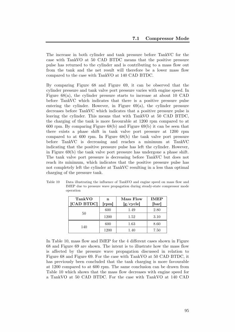
7.1 Compressor Mode
95
The increase in both cylinder and tank pressure before TankVC for the case with TankVO at 50 CAD BTDC means that the positive pressure pulse has returned to the cylinder and is contributing to a mass flow out from the tank and the net result will therefore be a lower mass flow compared to the case with TankVO at 140 CAD BTDC.
By comparing Figure 68 and Figure 69, it can be observed that the cylinder pressure and tank valve port pressure varies with engine speed. In Figure 68(a), the cylinder pressure starts to increase at about 10 CAD before TankVC which indicates that there is a positive pressure pulse entering the cylinder. However, in Figure 69(a), the cylinder pressure decreases before TankVC which indicates that a positive pressure pulse is leaving the cylinder. This means that with TankVO at 50 CAD BTDC, the charging of the tank is more favourable at 1200 rpm compared to at 600 rpm. By comparing Figure 68(b) and Figure 69(b) it can be seen that there exists a phase shift in tank valve port pressure at 1200 rpm compared to at 600 rpm. In Figure 68(b) the tank valve port pressure before TankVC is decreasing and reaches a minimum at TankVC indicating that the positive pressure pulse has left the cylinder. However, in Figure 69(b) the tank valve port pressure has undergone a phase shift. The tank valve port pressure is decreasing before TankVC but does not reach its minimum, which indicates that the positive pressure pulse has not completely left the cylinder at TankVC resulting in a less than optimal charging of the pressure tank.
Table 10 Data illustrating the influence of TankVO and engine speed on mass flow and IMEP due to pressure wave propagation during steady-state compressor mode operation
TankVO [CAD BTDC]
n [rpm]
Mass Flow [g/cycle]
IMEP [bar]
50 600 1.49 2.80
1200 1.52 3.10
140 600 1.63 8.60 1200 1.40 7.50
In Table 10, mass flow and IMEP for the 4 different cases shown in Figure 68 and Figure 69 are shown. The intent is to illustrate how the mass flow is affected by the pressure wave propagation discussed in relation to Figure 68 and Figure 69. For the case with TankVO at 50 CAD BTDC, it has previously been concluded that the tank charging is more favourable at 1200 compared to at 600 rpm. The same conclusion can be drawn from Table 10 which shows that the mass flow decreases with engine speed for a TankVO at 50 CAD BTDC. For the case with TankVO at 140 CAD

7 Results
96
BTDC it was previously concluded that the tank charging was more favourable at 600 rpm compared to at 1200 rpm. Once again, the same conclusion can be drawn from Table 10, which shows that the mass flow decreases with engine speed. However, it should be noted that this increase in mass flow at 600 rpm comes with the price of a higher IMEP.
7.1.6 Load Control
The results in previous sections have shown the influence of different parameters on compressor mode performance. With the help of these results it is possible to choose the parameter in such a manner that the compressor mode performance is maximized. However, in a real application, the choice of parameters will be entirely determined by the driving conditions and not by what is currently optimal with regards to pneumatic hybrid engine efficiency. During a braking event, the driver will be given the ability to control the degree of braking power by pressing the brake pedal. This motivates the purpose of the present sub-section. The ability to control the amount of braking power at a specific time is a very important aspect of the pneumatic hybrid concept. Ideally, a certain braking power should be achievable whatever the pressure level in the tank is. With all this in mind, a control strategy that controls the braking power of the pneumatic hybrid engine during compressor mode operation was developed.
Load Control at Steady-State Tank Pressure
The performance of a controller can be determined by observing the process response to a set point change. Parameters such as rise time, overshoot and settling time can be used in order to verify the controller performance. The controller used in the present study consists of a PID controller combined with a feedforward filter.
In Figure 9 it was shown that, pure feedforward control introduces large control errors due to different factors already discussed in connection to the figure. By adding a PID controller to the control system, this control error could be eliminated or at least decreased to reasonable levels. The results can be seen in Figure 70, where the process responds to a positive set point change between 4 and 5 bar IMEP and to a negative set point change between 8 and 4 bar, respectively, are shown. In Figure 70(a) it can be seen that the control error present in Figure 9 is now eliminated, both before and after the set point change. There is almost no overshoot and the process variable settles within 3 engine revolutions. The response to the negative set point change in Figure 70(b) shows no signs of a control error. The rise time and settling time are comparable to what was

7.1 Compressor Mode
97
shown in Figure 70(a). The conclusion of the results in Figure 70 is that the performance of the chosen control strategy is satisfactory with low rise time and settling time, no matter the direction or the magnitude of the set point change.
Figure 70 also shows the most important control variables, namely the tank valve opening and the tank valve duration. In Figure 70(a) it can be seen that the TankVO is advanced during the transient. The reason is that in order to achieve higher loads during compressor mode operation, the tank valve should open earlier in order to create a blowdown of compressed air from the tank into the cylinder and thus increase the negative IMEP. The earlier the TankVO occurs the greater the difference between cylinder and tank pressure, with an increase in negative IMEP as a result. The procedure is the same during a negative change in load, only now the TankVO is retarded during the set point change.
(a) (b) Figure 70 Closed loop process response to a set point change in IMEP during
compressor mode operation at a steady-state tank pressure; (a) Positive set point change from 4 to 5 bar, tank pressure=8 bar (b) Negative set point change from 8 to 4 bar, tank pressure=10 bar.
Figure 71 displays the process response during several set point changes in the form of a staircase. The intention is to illustrate a more realistic increase/decrease in IMEP between 4 and 7 bar during a braking event. In a real application, a too large sudden change in braking power during compressor mode operation might lead to transmission failure and therefore there exists a need for a more smooth transition. In the present case the set point is changed with an increment of 1 bar IMEP and a separation of about 50 engine revolutions between the set point changes. The controller has no problems controlling the process response. The rise
4
4.25
4.5
4.75
5
IME
P [b
ar]
MeasuredSetpoint
80
86
92
98
104
Ta
nkV
O [C
AD
BT
DC
]
100 150 200 250 300104
110
116
122
128
Ta
nkD
ur
[CA
D]
Engine Cycles [-]
4
5
6
7
8
IME
P [b
ar]
MeasuredSetpoint
60
80
100
120
140
Ta
nkV
O [C
AD
BT
DC
]100 150 200 250 300
90
110
130
150
170
Ta
nkD
ur
[CA
D]
Engine Cycles [-]
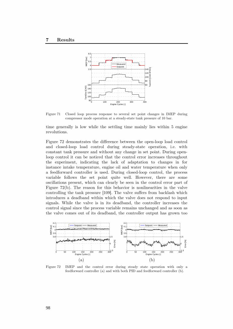
7 Results
98
Figure 71 Closed loop process response to several set point changes in IMEP during
compressor mode operation at a steady-state tank pressure of 10 bar.
time generally is low while the settling time mainly lies within 5 engine revolutions.
Figure 72 demonstrates the difference between the open-loop load control and closed-loop load control during steady-state operation, i.e. with constant tank pressure and without any change in set point. During open-loop control it can be noticed that the control error increases throughout the experiment, indicating the lack of adaptation to changes in for instance intake temperature, engine oil and water temperature when only a feedforward controller is used. During closed-loop control, the process variable follows the set point quite well. However, there are some oscillations present, which can clearly be seen in the control error part of Figure 72(b). The reason for this behavior is nonlinearities in the valve controlling the tank pressure [109]. The valve suffers from backlash which introduces a deadband within which the valve does not respond to input signals. While the valve is in its deadband, the controller increases the control signal since the process variable remains unchanged and as soon as the valve comes out of its deadband, the controller output has grown too
(a) (b) Figure 72 IMEP and the control error during steady state operation with only a
feedforward controller (a) and with both PID and feedforward controller (b).
2.5
4
5.5
7
8.5
IME
P [b
ar]
MeasuredSetpoint
60
80
100
120
140
Ta
nkV
O [C
AD
BT
DC
]
0 100 200 300 40080
100
120
140
160T
an
kDu
r [C
AD
]
Engine Cycles [-]
3.8
3.9
4
4.1
4.2
IME
P [b
ar]
Setpoint Measured
0 50 100 150 200 250 300-1.5
0
1.5
Err
or
[%]
Engine Cycles [-]
3.8
3.9
4
4.1
4.2
IME
P [b
ar]
Setpoint Measured
0 50 100 150 200 250 300-1.5
0
1.5
Err
or
[%]
Engine Cycles [-]

7.1 Compressor Mode
99
large which leads to excessive valve movement with an overshoot in process variable response as a result.
Load Control at Transient Tank Pressure
Above the performance of the suggested controller for steady-state tank pressure was demonstrated. However, in a real application the tank pressure will increase during a braking event. Therefore, the ability of the controller to reject disturbances has been tested. In the present case, the disturbance is introduced as a ramp-like increase in tank pressure. Figure 73(a) displays how the controller reacts to a disturbance in tank pressure. It can be noticed that there exists a bump in the process variable response immediately after the disturbance has been introduced. However, the controller manages to reject the disturbance eventually. The maximum control error observed is less than 2% which corresponds to less than 0.1 bar IMEP.
(a) (b) Figure 73 (a) A ramp-like change in tank pressure and its effect on the control of IMEP,
(b) A combination of load steps and a ramp change in tank pressure. The vertical solid line denotes the start of change in tank pressure.
In Figure 73(a), the goal was to keep the process variable, i.e. the load, at a constant level. However, during a braking event the braking power demand will most likely vary and thus the compressor mode load demand will also vary. In an attempt to test the controller during more realistic conditions, a sequence of set point changes in addition to the disturbance in tank pressure have been introduced. The results can be seen in Figure 73(b). Again, the controller manages to maintain the process variable at the desired set point despite the disturbance in tank pressure indicating
3
3.25
3.5
3.75
4
IME
P [b
ar]
MeasuredSetpoint
4
6
8
10
12
Ta
nk
Pre
ssu
re [b
ar]
40
55
70
85
100
Ta
nkV
O [C
AD
BT
DC
]
0 200 400 600 80080
90
100
110
120
Ta
nkD
ur
[CA
D]
Engine Cycles [-]
3
4
5
6
7
IME
P [b
ar]
MeasuredSetpoint
5
7
9
11
13
Ta
nk
Pre
ssu
re [b
ar]
40
60
80
100
120
Ta
nkV
O [C
AD
BT
DC
]
0 200 400 600 80070
90
110
130
150T
an
kDu
r [C
AD
]
Engine Cycles [-]

7 Results
100
its suitability during more realistic driving conditions. The maximum control error is again less than 2%.
7.2 Air-Motor Mode
The Air-Motor Mode is the mode during which the ICE is used as a 2-stroke air-motor. As with the compressor mode, the air-motor mode can be executed in three ways: with emphasis on optimal efficiency, maximum power or a trade-off between both. In the following sub-sections results from basic and optimal air-motor operation will be shown followed by modeling of the air-motor mode in GT-power and a parametric study similar to the one described in Section 7.1.5.
7.2.1 Initial Testing of Air-Motor Mode
The intention with the present sub-section is to demonstrate the basics of air-motor mode. It serves as an introduction to the following section on optimal air-motor operation.
Table 11 Valve timings during initial testing of air-motor operation
IVO 180 CAD BTDC IVC 0 CAD ATDC TankVO 5 CAD ATDC TankVC 40 CAD ATDC
During the experiments presented in this sub-section constant valve timings were used, see Table 11. By setting IVO at BDC and IVC at TDC, there will be no compression of the air in the cylinder during the compression stroke. The reason is that the compression of air during the compression stroke would lead to a high pressure at TDC making it hard for the tank valve to open at the desired CAD. Due to nonlinearities in the pneumatic valve actuator, the real opening and closing of the valve is not always as desired. Therefore the tank valve is set to open 5 CAD ATDC and by doing so the risk of creating a flow of compressed air from the pressure tank directly out through the inlet port can be prevented. The reason why TankVC was set to 40 CAD ATDC is that at a high tank pressure the tank valve should close relatively near TDC in order to prevent the generation of excessively large driving power.
Figure 74 shows the PV-diagram of one air-motor cycle during real engine testing at two different tank pressures. Comparing the PV-diagrams in

7.2 Air-Motor Mode
101
Figure 74 to the ideal PV-diagram in Figure 11(b) indicates that there is a significant difference. In Figure 11(b), the pressure between TankVO and TankVC, which is known as the charging period, is constant. This means that when the tank valve opens, the pressurized air fills the cylinder instantly and the charging of the cylinder continues at the same pressure until the tank valve closes. However, in Figure 74 a decrease in cylinder pressure between TankVO and TankVC can be noticed. The reason for this behavior is flow restrictions across the tank valve. A restriction in flow of pressurized air from the tank into the cylinder during the expansion stroke will lead to the fact that the cylinder cannot be filled with enough pressurized air in order to maintain the same pressure level throughout the charging period.
Further comparison between Figure 11(b) and Figure 74 indicates that the latter lacks the compression step between IVC and TankVO. The reason is inappropriate IVC. In the present case IVC has been chosen to occur at TDC which results in a cylinder pressure at about atmospheric level when TankVO occurs and thus there will be a blowdown of pressurized air from the tank into the cylinder with high pressure loss as a result. If IVC is controlled in such a way that the air trapped in the cylinder after IVC is compressed to the same level as the tank pressure prior to TankVO, the blowdown of pressurized air into the cylinder can be avoided.
(a) (b) Figure 74 Cylinder pressure during air-motor operation as a function of cylinder volume
illustrated in the form of a PV-diagram at a tank pressure of 13 bar (a) and 7 bar (b), respectively.
Another thing that can be observed in Figure 74(b) is that the PV-diagram consists of two enclosed loops. The loop on the left side of the figure is a positive loop during which the pressurized air contributes with positive work. The loop on the right side of the figure is a negative loop which contributes with negative IMEP and the reason for its occurrence is
0 0.5 1 1.5 2 2.50
2
4
6
8
10
12
Cylinder Volume [dm3]
Cyl
ind
er
Pre
ssu
re [b
ar]
TankPressure 13 bar
0 0.5 1 1.5 2 2.50
1
2
3
4
5
6
Cylinder Volume [dm3]
Cyl
ind
er
Pre
ssu
re [b
ar]
TankPressure 7 bar

7 Results
102
unsuitable valve timings. The amount of pressurized air introduced into the cylinder during the charging period is not enough in order for the pressure to reach ambient pressure at the end of the expansion stroke. Instead the cylinder pressure will decrease below atmospheric pressure and thus vacuum will be created which is an energy consuming process. Since the IVO occurs at BDC, the vacuum will be cancelled by the induction of fresh air into the cylinder and thereby the vacuum previously created cannot be used as an upward-acting force on the piston as it moves towards TDC. There are basically two ways to prevent this occurrence. One is to postpone IVO until the cylinder pressure reaches atmospheric pressure as the piston travels towards TDC. The second way is to have longer tank valve duration and thus induct more pressurized air into the cylinder during the charging period. In this way the cylinder pressure will reach atmospheric pressure at BDC and the inlet valve can then open at BDC.
(a) (b)
Figure 75 Positive IMEP (a) and tank pressure (b) as a function of engine cycle number during transient air-motor operation.
Figure 75 shows the positive IMEP and tank pressure during 400 consecutive engine cycles of transient air-motor operation. The tank pressure starts at about 20 bar and after 400 engine cycles it has decreased to about 5 bar. During this period the IMEP goes from about 3.8 bar down to 0 bar. This raises the question why IMEP reaches 0 bar while the corresponding tank pressure is still above ambient pressure. The question can be answered with the help of Figure 76 where the negative loop of the PV-diagram has grown to such extent that it is now as large as the positive loop. This means that the power input has reached the same level as the power output and the net result will therefore be an IMEP of 0 bar. The air-motor mode efficiency can be seen in Figure 77. It verifies what has been discussed in connection with Figure 75. The air-
0 100 200 300 4000
0.8
1.6
2.4
3.2
4
Number of Engine Cycles
Po
sitiv
e IM
EP
[ba
r]
0 100 200 300 400
5
10
15
20
25
Number of Engine Cycles
Me
an
Ta
nk
Pre
ssu
re [b
ar]

7.2 Air-Motor Mode
103
Figure 76 PV-diagram illustrating the occurrence of an IMEP of 0 bar at a tank pressure of 5 bar.
Figure 77 The air-motor mode efficiency, ηAM, as a function of engine cycle number during transient air-motor mode.
motor mode efficiency is defined as the ratio between the energy recovered during air-motor mode and the energy consumed in the form of compressed air. It has been shown that the recovered energy, EAM, can be expressed as a function of IMEP. An IMEP of 0 bar consequently means that EAM is alos 0, which results in a ηAM of 0% as shown in Figure 77. The ηAM,tot is the accumulated efficiency over 400 engine cycles and in the present case it reaches 34.2%.
7.2.2 Optimal Air-Motor Mode Operation
In this sub-section, optimization of the air-motor mode will be presented. The optimization has been done in terms of valve timings and valve head diameter.
During the optimization of the compressor mode described in Section 7.1.2, proper valve timings were determined at steady-state conditions.
0 0.5 1 1.5 2 2.50
0.5
1
1.5
2
2.5
3
3.5
4
Cylinder Volume [dm3]
Cyl
ind
er
Pre
ssu
re [b
ar]
TankPressure 5 bar
0 100 200 300 4000
10
20
30
40
50
Number of Engine Cycles
Air
Mo
tor
Mo
de
Effi
cie
ncy
[%]
AM,tot
=34.2%

7 Results
104
This means that the pressure in the tank was held at a constant level and by varying the valve timings an optimal setting could be found for that particular tank pressure. However, during air-motor mode the same approach would require the tank to be fed with pressurized air from an external source in order to maintain a constant pressure. An external source, capable of generating compressed air at a pressure as high as 20 bar while supplying the required mass flow, was at the time of the experimental work not available. Therefore a different strategy had to be used.
In Section 7.1.1 it was shown how proper valve timings could be calculated theoretically with the help of the polytropic compression equation(7.1). The same approach was applied for the air-motor mode. The TankVC and corresponding positive IMEP obtained with this method as a function of tank pressure can be seen in Figure 78(a). IMEP is very low, almost below 1 bar for all tank pressures, which leads to the conclusion that the method might not be suitable for air motor mode optimization. The problem is most likely the fact that the polytropic relation does not take the flow restrictions across the valve into account. When using the abovementioned method to calculate the valve timings it is assumed that the cylinder is filled with compressed air in an instant. However, due to the flow restriction the time it takes to fill the cylinder with the required amount of compressed air will be longer and hence by using the polytropic relation the TankVC will be chosen closer to TDC than optimal.
(a) (b)
Figure 78 TankVC and corresponding positive IMEP as a function of tank pressure; (a) Theoretically calculated TankVC, (b) TankVC based on results from optimized compressor mode
Since the method described above was recognized as unsuitable, there was a need to find an alternative method in order to determine optimal valve
051015200
45
90
135
180
Ta
nkV
C [C
AD
AT
DC
]
Tank Pressure [bar]
051015200
1
2
3
4
Po
sitiv
e IM
EP
[ba
r]TankVCPositive IMEP
05101520250
45
90
135
180
Ta
nkV
C [C
AD
AT
DC
]
Tank Pressure [bar]
05101520250
1
2
3
4P
osi
tive
IME
P [b
ar]
TankVCPositive IMEP
7.2 Air-Motor Mode
105
timings. Two methods were developed, one for determining proper IVC and one for determining proper TankVC.
In Section 3.2 it was established that optimal IVC should occur so that the cylinder pressure at TDC equals the tank pressure. By varying IVC the corresponding cylinder pressure at TDC will also vary. In this way, a map of IVC as a function of peak cylinder pressure can be created.
In order to find optimal TankVC, results from optimal compressor mode shown in Figure 48 was used. When operating the compressor mode optimally, the air in the cylinder is compressed during the compression stroke to the same pressure level as the tank pressure level prior to TankVO. During air-motor mode the procedure should be the opposite. The charging period starts with TankVO at TDC. As the piston moves away from TDC, the compressed air will expand into the cylinder and when the pressure in the cylinder equals the pressure in the tank, the tank valve should close. This means that TankVO during compressor mode corresponds to TankVC during air-motor mode in terms of CAD BTDC and ATDC, respectively. During compressor mode the tank valve opens when pressure equilibrium is reached and during air-motor mode the tank valve closes at the same condition. Thereby, the results obtained during compressor mode optimization, can be used to control the tank valve during air-motor mode. For instance, if it is determined that TankVO during compressor mode operation should occur at 35 CAD BTDC, then TankVC during air-motor mode should occur at 35 CAD ATDC. The results can be seen in Figure 78(b). By comparing Figure 78(a) and Figure 78(b) it can clearly be seen that there is a considerable difference in TankVC and IMEP between the two methods. For instance at a tank pressure of 15 bar, the TankVC obtained with the polytropic relation occurs at 22 CAD ATDC while the corresponding TankVC for the compressor mode based method occurs at 37 CAD ATDC and the result is a difference of 15 CAD between the two methods.
In Figure 79, negative IMEP and corresponding tank pressure for both unoptimized (see Table 11) and optimized valve timings during transient air-motor operation can be seen. It should be noted that for the optimal case, the valve diameter has been increased (from 16 to 28 mm) in addition to the optimization of the valve timings. Unfortunately, no data for the optimized case prior to the change in valve diameter exists due to data acquisition error.
The difference between the unoptimized and the optimized case with regards to both tank pressure and positive IMEP in Figure 79 is

7 Results
106
considerable. During the optimized case, the IMEP is above 0 bar as long as the tank pressure is above atmospheric pressure, which indicates a
(a) (b)
Figure 79 Comparison of transient air-motor operation with unoptimized and optimized valve timings: (a) Negative IMEP as a function of engine cycle number; (b) Tank pressure as a function of engine cycle number.
much more efficient use of the pressurized air, which is confirmed by Figure 80. The total air-motor mode efficiency for the optimized case has been improved by 24.8 percentage points compared to the unoptimized case, which corresponds to an improvement by about 73%. It should be remembered however, that not only the optimized valve timings but also the increase in valve diameter contributes to this improvement. A larger tank valve diameter contributes to less pressure losses over the tank valve while an optimized valve timing strategy contributes to a more efficient use of the pressurized air. Both these parameters are key to efficient air-motor operation.
Figure 80 The air-motor efficiency during transient air-motor operation with theoretical and optimized valve timings.
0 100 200 300 400 5000
0.5
1
1.5
2
2.5
3
3.5
4
Number of Engine Cycles
Po
sitiv
e IM
EP
[ba
r]
UnoptimizedOptimized
0 100 200 300 400 5000
5
10
15
20
25
Number of Engine CyclesT
an
k P
ress
ure
[ba
r]
UnoptimizedOptimized
0 100 200 300 400 5000
20
40
60
80
100
Number of Engine Cycles
Air
Mo
tor
Mo
de
Effi
cie
ncy
[%]
Optimized AM,AM,tot
= 59.0%
Unoptimized AM, AM,tot
= 34.2%
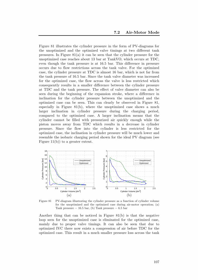
7.2 Air-Motor Mode
107
Figure 81 illustrates the cylinder pressure in the form of PV-diagrams for the unoptimized and the optimized valve timings at two different tank pressures. In Figure 81(a) it can be seen that the cylinder pressure for the unoptimized case reaches about 13 bar at TankVO, which occurs at TDC, even though the tank pressure is at 16.5 bar. This difference in pressure occurs due to flow restrictions across the tank valve. For the optimized case, the cylinder pressure at TDC is almost 16 bar, which is not far from the tank pressure of 16.5 bar. Since the tank valve diameter was increased for the optimized case, the flow across the valve is less restricted which consequently results in a smaller difference between the cylinder pressure at TDC and the tank pressure. The effect of valve diameter can also be seen during the beginning of the expansion stroke, where a difference in inclination for the cylinder pressure between the unoptimized and the optimized case can be seen. This can clearly be observed in Figure 81, especially in Figure 81(b), where the unoptimized case shows a much larger inclination in cylinder pressure during the charging period, compared to the optimized case. A larger inclination means that the cylinder cannot be filled with pressurized air quickly enough while the piston moves away from TDC which results in a decrease in cylinder pressure. Since the flow into the cylinder is less restricted for the optimized case, the inclination in cylinder pressure will be much lower and resemble the isobaric charging period shown for the ideal PV diagram (see Figure 11(b)) to a greater extent.
(a) (b) Figure 81 PV-diagram illustrating the cylinder pressure as a function of cylinder volume
for the unoptimized and the optimized case during air-motor operation; (a) Tank pressure = 16.5 bar, (b) Tank pressure = 6.5 bar
Another thing that can be noticed in Figure 81(b) is that the negative loop seen for the unoptimized case is eliminated for the optimized case, mainly due to proper valve timings. It can also be seen that due to optimized IVC there now exists a compression of air before TDC for the optimized case. This result in a much smaller pressure loss across the tank
0 0.5 1 1.5 2 2.50
2
4
6
8
10
12
14
16
18
Cylinder Volume [dm3]
Cyl
ind
er
Pre
ssu
re [b
ar]
UnoptimizedOptimized
0 0.5 1 1.5 2 2.50
1
2
3
4
5
6
7
Cylinder Volume [dm3]
Cyl
ind
er
Pre
ssu
re [b
ar]
UnoptimizedOptimized

7 Results
108
valve and consequently the consumption of pressurized air from the tank can be decreased thus increasing the air-motor mode efficiency.
7.2.3 Air-Motor Mode Modeling in GT-Power
In Section 7.1.4 the validation of a compressor mode model developed in GT-power was presented. In the present section, validation of an equivalent air-motor mode model against measured data will be shown. Since measured steady-state data from air-motor operation are not available due to reasons mentioned earlier, the focus in this section is on transient air-motor mode operation. The air-motor mode model is basically the same as the compressor mode model and the main difference lies in the valve timings.
In Figure 82, positive IMEP during transient air-motor operation is presented. The simulated curve reproduces the shape of the measured data very well with a relative error mainly within 5% which is in accordance with the corresponding results during compressor mode operation shown in Figure 54.
Figure 82 Positive IMEP and corresponding relative error as a function of engine cycle number during measured and simulated transient air-motor operation at an engine speed of 600 rpm.
Figure 83(a) shows the mean tank pressure during transient air-motor operation. The relative error in this case ranges from 0 to a little over 40%. In spite of this, it can be noticed that the simulated results follow the trend of the measured results. The poor agreement between predicted and measured data can be explained with references to Figure 83(b) which displays the tank valve port temperature. It can be seen that the initial temperature for the simulated data is much lower compared to the measured data. The difference in incline between measured and predicted data indicates that the heat transfer needs additional tuning. The considerable difference in temperature between the simulated and
0
1
2
3
4
Po
sitiv
e IM
EP
[ba
r]
MeasGTP
0 100 200 300 400 500-10010
Number of Engine Cycles
x [%
]

7.2 Air-Motor Mode
109
measured data is what causes the difference in mean tank pressure shown in Figure 83(a). The incline in temperature means that the pressure in the tank will decrease, not only because it is used for motoring the engine, but also because of cooling of the hot pressurized air contained in the tank and the pipe connecting it to the cylinder head. Since the temperature
(a) (b) Figure 83 Mean tank pressure (a) and tank valve port temperature (b) together with
corresponding relative error as a function of engine cycle number during measured and simulated air-motor mode operation at an engine speed of 600 rpm.
decreases at a higher rate for the measured data compared to simulated, the tank pressure does the same and this is the reason why simulated tank pressure is higher than measured tank pressure during air-motor mode operation.
7.2.4 Parametric Study of Air-Motor Mode Performance
The results shown in the previous section are not satisfactory. The model needs additional tuning. However, it might still serve as an indicator of how different parameters affect the performance of air-motor mode.
Tank Valve Diameter
Above, the valve diameter was identified as an important factor with regards to compressor mode performance since it affects the mass flow across the tank valve to a great extent. In Section 7.2.2 it was shown that an increase in valve diameter together with optimal valve timings leads to a significant improvement in air-motor mode efficiency. However, it is unclear how much of the improvement can be attributed to a larger tank valve and to a more optimal valve strategy, respectively. Therefore, in this section the effect of valve diameter on air-motor mode operation will be investigated.
0
5
10
15
20
25
Me
an
Ta
nk
Pre
ssu
re [b
ar]
MeasGTP
0 100 200 300 400 50003060
Number of Engine Cycles
x [%
] 300
350
400
450
500
550
Ta
nk
Va
lve
Po
rt T
em
pe
ratu
re [K
]
MeasGTP
0 100 200 300 400 500-40-200
Number of Engine Cycles
x [%
]

7 Results
110
In Figure 84 and Figure 85, the results from transient air-motor mode operation for two different valve configurations at 600 and 1200 rpm, respectively, can be seen. The negative mass flow indicates that the flow goes from the tank into the cylinder. At 600 rpm, the mass flow is initially higher for the 32 mm setup, compared to the 16 mm setup which indicates that the mass flow is less restricted with a larger valve diameter, see Figure 84(b). A higher mass flow results in a higher IMEP due to a higher amount of pressurized air charged into the cylinder during the charging period, see Figure 84(a). After about 230 engine cycles, both IMEP and mass flow becomes larger for the 16 mm setup compared to the 32 mm setup. The reason is that the tank pressure has reached a much lower level for the larger valve setup at that point and there is not enough pressurized air to maintain the mass flow at a higher level.
The total air-motor mode efficiency for the 16 mm and 32 mm setup at 600 rpm is 41.9% and 43.6%, respectively. This corresponds to an increase in efficiency by about 4.1%, when switching from 16 mm to 32 mm in tank valve diameter. Comparing these results to the results shown in Figure 80 clearly indicates that a larger valve diameter has a very limited influence on the total improvement in air-motor mode efficiency at 600 rpm.
In Figure 85 it can be seen that the difference in initial mass flow between the two valve setups has increased at 1200 rpm compared to the case at 600 rpm. The initial mass flow for the 16 mm setup is about 4.2 g/cycle at 600 rpm and about 2.1 g/cycle at 1200 rpm. This means that by doubling the engine speed, the mass flow is lowered by 50% for the 16 mm setup which clearly indicates the restriction in mass flow. On the other hand, the mass flow for the 32 mm setup is about 5.8 g/cycle at 600 rpm and
(a) (b)
Figure 84 Transient air-motor operation for two different valve setups at an engine speed of 600 rpm; (a) Positive IMEP, (b) Mass flow and tank pressure.
0 100 200 300 400 5000
1
2
3
4
5
Number of Engine cycles [-]
Po
sitiv
e IM
EP
[ba
r]
=16mm, AM,tot
=41.9%
=32mm, AM,tot
=43.6%
0 100 200 300 400 500-6
-4.8
-3.6
-2.4
-1.2
0
Ma
ss F
low
[g/c
ycle
]
Number of Engine Cycles [-]
0 100 200 300 400 5000
5
10
15
20
25
Ta
nk
Pre
ssu
re [b
ar]
0 100 200 300 400 5000
5
10
15
20
25=16mm=32mm

7.2 Air-Motor Mode
111
(a) (b) Figure 85 Transient air-motor operation for two different valve setups at an engine speed
of 1200 rpm; (a) Positive IMEP, (b) Mass flow and tank pressure.
about 5 g/cycle at 1200 rpm, which corresponds to a decrease by about 14%. The restriction of mass flow for the 16 mm valve at 1200 rpm leads to very low air-motor mode efficiency, in this case 16.9%. The corresponding efficiency for the 32 mm setup is 33.5% which indicates that a larger valve diameter is key to high efficiency at higher engine speeds.
Tank Valve Closing
TankVC is probably the most important parameter influencing the performance of the air-motor mode operation. It controls the flow of pressurized air into the cylinder and determines how much positive power will be generated at a given tank pressure. Figure 86 shows how IMEP and mass flow varies with TankVC at two different engine speeds. It can be seen that both IMEP and mass flow increases with TankVC. By moving TankVC away from TDC, the charging period is increased which means that the cylinder will be charged with pressurized air from the tank during a longer period and consequently the mass flow will increase which in turn results in a higher IMEP. There is a significant difference between the results at 600 and 1200 rpm. Both IMEP and mass flow is lower for the case at 1200 rpm compare to the case at 600 rpm. The reason is that the time between TDC and TankVC decreases with engine speed even though the crank angle at which TankVC occurs remains constant. However, the flow of pressurized air from the tank into the cylinder does not depend on engine speed and remains constant with respect to time. This is not entirely true since the flow out from the tank can be influenced by pressure wave propagation and by the downward motion of the piston. For instance, a mass flow of 6 g/cycle occurs at a TankVC of 30 CAD ATDC for the case at 600 rpm which corresponds to a charging period of about 8 ms. The statement that the mass flow does not depend
0 100 200 300 400 5000
1
2
3
4
5
Number of Engine cycles [-]
Po
sitiv
e IM
EP
[ba
r]
=16mm, AM,tot
=16.9%
=32mm, AM,tot
=33.5%
0 100 200 300 400 500-6
-4.8
-3.6
-2.4
-1.2
0
Ma
ss F
low
[g/c
ycle
]
Number of Engine Cycles [-]
0 100 200 300 400 5000
5
10
15
20
25
Ta
nk
Pre
ssu
re [b
ar]
0 100 200 300 400 5000
5
10
15
20
25
=16mm=32mm

7 Results
112
on engine speed means that the equivalent TankVC at which the mass flow is 6 g/cycle at an engine speed of 1200 rpm would therefore occur at 60 CAD ATDC. However, at 1200 rpm, a mass flow of 6 g/cycle occurs at about 36 CAD ATDC which corresponds to a charging period of 5 ms. The difference in charging period is thus about 3 ms which clearly indicates that there are other factors influencing the mass flow.
Figure 86 Mass flow and positive IMEP as a function of TankVC at a tank pressure of 20 bar and two different engine speeds.
In Figure 87 and Figure 88 the results from transient air-motor operation for three different TankVC at 600 and 1200 rpm, respectively, are displayed. In Figure 87 it can be seen that a late TankVC leads to a high initial IMEP at the expense of a higher mass flow and thus a higher rate of tank pressure depletion. It can also be seen that the air- motor mode efficiency, ηAM, varies with TankVC. The reason why the TankVC at 20 CAD ATDC displays the lowest air-motor mode efficiency is that the charging of the cylinder is insufficient which leads to the creation of a
(a) (b)
Figure 87 Transient air-motor operation for three different TankVC at an engine speed of 600 rpm; (a) Positive IMEP, (b) Mass flow and tank pressure.
0 10 20 30 40 50 600
2
4
6
8
10
Ma
ss F
low
[g/c
ycle
]
TankVC [CAD ATDC]
0 10 20 30 40 50 600
3
6
9
12
Po
sitiv
e IM
EP
[ba
r]
0 10 20 30 40 50 600
3
6
9
12600 rpm1200 rpm
0 100 200 300 400 5000
2
4
6
8
10
Number of Engine cycles [-]
Po
sitiv
e IM
EP
[ba
r]
TankVC=20, AM,tot
=34.5%
TankVC=40, AM,tot
=44.3%
TankVC=60, AM,tot
=43.3%
0 100 200 300 400 500-15
-12
-9
-6
-3
0
Ma
ss F
low
[g/c
ycle
]
Number of Engine Cycles [-]
0 100 200 300 400 5000
5
10
15
20
25
Ta
nk
Pre
ssu
re [b
ar]
0 100 200 300 400 5000
5
10
15
20
25
0 100 200 300 400 5000
5
10
15
20
25
TankVC=20TankVC=40TankVC=60

7.2 Air-Motor Mode
113
(a) (b) Figure 88 Transient air-motor operation for three different TankVC at an engine speed
of 1200 rpm; (a) Positive IMEP, (b) Mass flow and tank pressure.
negative IMEP, see Figure 74.
By comparing Figure 87 and Figure 88, it can be observed that the IMEP at 1200 rpm is much lower compared to the corresponding IMEP at 600 rpm. This behavior is in analogy with Figure 86, where it was established that the mass flow of pressurized air into the cylinder is independent of engine speed and to some extent influenced by pressure wave propagation. The mass flow at 1200 rpm is lower compared to the corresponding mass flow at 600 rpm, and therefore a lower IMEP at 1200 rpm can be expected. Another reason for the lower IMEP is that at higher engine speed, the charging period constitutes a larger part of the expansion stroke and thus leaves a shorter pure expansion stroke, i.e the part of the expansion during which all valves are closed. With a shorter expansion stroke, less energy will be converted to positive work and thus positive IMEP will decrease.
Inlet Valve Closing
When taking air-motor mode efficiency into consideration, IVC should occur in such a way that the cylinder pressure at TDC reaches the same level as the tank pressure. In this way the charging of the cylinder after TDC will be executed smoothly with less pressure losses.
In Figure 89(a) the influence of IVC on mass flow and IMEP during steady-state air-motor mode operation for two engine speeds is displayed. It can be seen that both mass flow and IMEP decrease with advancing IVC. The positive IMEP decreases with advancing IVC since the degree of compression of the air trapped in the cylinder increases with advancing IVC. This in turn results in an increase in negative work and the net positive work for the entire cycle thus be decreases. The mass flow
0 100 200 300 400 5000
2
4
6
8
10
Number of Engine cycles [-]
Po
sitiv
e IM
EP
[ba
r]
TankVC=20, AM,tot
=22.6%
TankVC=40, AM,tot
=33.8%
TankVC=60, AM,tot
=34.3%
0 100 200 300 400 500-15
-12
-9
-6
-3
0
Ma
ss F
low
[g/c
ycle
]
Number of Engine Cycles [-]
0 100 200 300 400 5000
5
10
15
20
25
Ta
nk
Pre
ssu
re [b
ar]
0 100 200 300 400 5000
5
10
15
20
25
0 100 200 300 400 5000
5
10
15
20
25
TankVC=20TankVC=40TankVC=60

7 Results
114
displays a similar trend to IMEP as IVC is advanced. A late IVC will lead to a very limited compression stroke and thus there will be a blowdown of pressurized air into the cylinder after TankVO occurs. This blowdown leads to unnecessarily high mass flow into the cylinder which results in a large pressure drop. With an IVC of about 60 CAD BTDC the air in the cylinder is compressed up to about 20 bar at TDC, which corresponds to the tank pressure in studied case. In this way the blowdown is eliminated
(a) (b)
Figure 89 Various parameters as functions of IVC at a tank pressure of 20 bar; (a) Mass flow and IMEP, (b) β - the ratio between IMEP and mass flow shown in (a).
which results in a lower mass flow and consequently lower pressure losses.
In Figure 89(b) a new parameter, β, is introduced. β is defined as the ratio between IMEP and mass flow:
AM
AM
IMEPβ=mflow
(7.3)
where mflowAM is the mass flow during air-motor mode. The parameter can be interpreted as the amount of IMEP generated per gram of pressurized air charged into the cylinder. In Figure 89(b) it can be seen that β increases with IVC at both engine speeds which means that the pressurized air is used more efficiently for a late IVC.
In Figure 90 and Figure 91 the results from transient air motor mode operation for three different IVC at 600 and 1200 rpm, respectively, are displayed. For the case with IVC at 50 CAD BTDC both IMEP and mass flow are initially lower compared to the remaining two cases. However, after a number of engine cycles the IMEP and mass flow become higher for the case with IVC at 50 CAD BTDC. The reason is that due to the lower mass flow, the pressurized air in the tank will last longer and thus
0 10 20 30 40 50 60-6
-5
-4
-3
-2
-1
Ma
ss F
low
[g/c
ycle
]
IVC [CAD BTDC]
0 10 20 30 40 50 600
1
2
3
4
5
Po
sitiv
e IM
EP
[ba
r]
0 10 20 30 40 50 600
1
2
3
4
5
600 rpm1200 rpm
0 10 20 30 40 50 600.5
0.6
0.7
0.8
0.9
1
IVC [CAD BTDC]
[b
ar/g
]
600 rpm1200 rpm

7.3 Drive cycle Simulations
115
contribute with positive work when the remaining cases have reached their limits.
(a) (b) Figure 90 Transient air-motor operation for three different IVC at an engine speed of
600 rpm; (a) Positive IMEP, (b) Mass flow and tank pressure.
(a) (b) Figure 91 Transient air-motor operation for three different IVC at an engine speed of
1200 rpm; (a) Positive IMEP, (b) Mass flow and tank pressure.
In Figure 90(a) and Figure 91(a) it can be seen that the total air-motor mode efficiency increases with IVC. The reason is that the β-ratio shown in Figure 89(b), increases with IVC which means that the pressurized air is used more efficiently and as a result the air-motor mode efficiency will also increase with IVC.
7.3 Drive cycle Simulations
The results shown in previous sections are all related to the pneumatic hybrid engine. Different parameters and their effects on the performance of the different pneumatic hybrid engine modes of operation have been thoroughly discussed. However, these results do not give a direct measure
0 100 200 300 400 5000
1
2
3
4
5
Number of Engine cycles [-]
Po
sitiv
e IM
EP
[ba
r]
IVC=10, AM,tot
=49.2%
IVC=30, AM,tot
=50.9%
IVC=50, AM,tot
=53.2%
0 100 200 300 400 500-5
-4
-3
-2
-1
0
Ma
ss F
low
[g/c
ycle
]Number of Engine Cycles [-]
0 100 200 300 400 5000
5
10
15
20
25
Ta
nk
Pre
ssu
re [b
ar]
0 100 200 300 400 5000
5
10
15
20
25
0 100 200 300 400 5000
5
10
15
20
25
IVC=10IVC=30IVC=50
0 100 200 300 400 5000
1
2
3
4
5
Number of Engine cycles [-]
Po
sitiv
e IM
EP
[ba
r]
IVC=10, AM,tot
=39.7%
IVC=30, AM,tot
=41.8%
IVC=50, AM,tot
=46.0%
0 100 200 300 400 500-5
-4
-3
-2
-1
0
Ma
ss F
low
[g/c
ycle
]
Number of Engine Cycles [-]
0 100 200 300 400 5000
5
10
15
20
25
Ta
nk
Pre
ssu
re [b
ar]
0 100 200 300 400 5000
5
10
15
20
25
0 100 200 300 400 5000
5
10
15
20
25
IVC=10IVC=30IVC=50

7 Results
116
of how a pneumatic vehicle will perfrom. Therefore, in this section results from vehicle simulations will be shown. A pneumatic hybrid bus was modeled in Simulink/Matlab and its performance over different drive cycles was investigated. The main intent was to explore the potential of the pneumatic hybrid bus regarding fuel consumption reduction compared to a traditional ICE powered bus.
7.3.1 Pneumatic Hybrid Performance Maps
An important part of the vehicle model is its engine-part. In the vehicle model used in this study, the pneumatic hybrid engine-part was implemented in the form of performance maps of both air-motor and compressor mode. These maps show the mass flow of air into or out from the tank (depending on the mode of operation) as a function of engine load and tank pressure. The performance maps for compressor mode and air-motor mode, respectively, can be seen in Figure 92. In Figure 92(a) it can be seen that during compressor mode operation the engine load (IMEP) can reach very high levels. At a tank pressure of 20 bar IMEP can become as high as 19 bar which corresponds to a brake torque of about 600 Nm. This indicates the high potential of compressor mode as a means of braking the vehicle.
It can further be seen in Figure 92(a) that the isolines display a wave-like behavior. At low tank pressures the isolines are almost parallel with the y-axis which in other words means that the mass flow at low tank pressures is almost independent of the load. However, at higher tank pressures the isolines transform into wave-like lines. This behavior can be attributed to pressure wave propagation in the pipeline connecting the pressure tank
(a) (b) Figure 92 Performance maps illustrating the mass flow rate (g/cycle) across the tank
valve as a function of both IMEP and tank pressure; (a) Compressor mode, (b) Air-motor mode
Tank Pressure [bar]
Ne
ga
tive
IME
P [b
ar]
1.8
1.61.4 1.2 1 0.8
5 10 15 20
5
10
15
20
Tank Pressure [bar]
Po
sitiv
e IM
EP
[ba
r]
2
4
6
8
10
5 10 15 20
1
2
3
4
5
6
7
8
9

7.3 Drive cycle Simulations
117
with the cylinder head.
Figure 92(b) displays how the mass flow depends on tank pressure and engine load during air-motor mode operation. It can be seen that the maximum engine load is limited to about 9.5 bar IMEP which corresponds to about 300 Nm of engine torque. This is about half of what was previously shown for the compressor mode. The reason why the engine load is limited during air-motor mode is not an inability to produce higher engine loads. The problem is that high engine load leads to very low air-motor mode efficiency. The higher the engine load, the higher the required amount of pressurized air which in turn means that the tank valve closing should occur later in the cycle. The result is that the cylinder pressure at IVO becomes higher than the inlet manifold pressure. Therefore, a blowdown of compressed air into the manifold will occur without any positive work being extracted from it which consequently leads to a decrease in air-motor mode efficiency. This can clearly be seen in Figure 93. At the time of inlet valve opening (point 3), the cylinder pressure is about 6 bar which will create a blowdown of pressurized air into the inlet manifold and at the time of inlet valve closing the pressure in the cylinder has decreased to the ambient pressure of 1 bar.
Figure 93 PV-diagram of one cycle during air-motor mode operation illustrating the blowdown of pressurized air through the inlet port at high engine loads.
7.3.2 Optimal Pressure Tank Volume
The pressure tank is a very important part of the model. Determining the optimal tank volume is a very important process since, the tank volume affects vehicle weight, total pneumatic hybridization cost and fuel consumption. For instance, an excessively large tank, will lead to a considerable increase in total vehicle weight with an increase in both cost and fuel consumption. The optimal size of the tank depends heavily on the type of driving cycle. However, choosing a very small tank might lead
0 0.5 1 1.5 2 2.50
5
10
15
20
25
Cylinder Volume [dm3]
Cyl
ind
er
Pre
ssu
re [b
ar]
Torque = 250 NmIMEP = 8.5 barTankPressure = 17.4 bar
4
3
21

7 Results
118
to a situation where a large portion of the energy recovered during compressor mode operation cannot be stored in the tank. This clearly indicates the importance of finding the proper tank size.
Figure 94 illustrates how the friction brake usage and mean tank pressure varies with tank pressure for two different drive cycles. The friction brake usage is defined as the ratio between the amount of brake energy generated by the friction brakes and the total brake energy demanded by the drive cycle. This parameter is directly related to the amount of time the powertrain will spend in compressor mode during the drive cycle. A low friction brake usage means that the main part of the braking power is generated form a high compressor mode activity. It can be seen in both figures that mean tank pressure decreases while friction brake usage increases with tank volume. The reason for this behavior is that the amount of energy that can be stored in the tank during the drive cycle is almost constant, independent of tank volume and since the amount of energy stored in the tank is a function of volume and pressure, the pressure in the tank will decrease with tank volume. With references to Figure 92(a), the decrease in tank pressure will lead to a decrease in maximum achievable brake torque during compressor mode which in turn limits the braking power generated during compressor mode operation and consequently the friction brake usage will increase.
(a) (b) Figure 94 Friction brake usage and mean tank pressure as a function of tank volume for
two different drive cycles; (a) FIGE drive cycle, (b) New York Composite drive cycle.
The results in Figure 94 indicate that the tank volume should be chosen as small as possible in order to minimize the friction brake usage. However, this is true for the compressor mode but not necessarily for the air-motor mode. A small tank means that the maximum amount of energy that can be stored in the tank is limited. This means that even if the amount of energy stored during compressor mode is at a maximum, there
0 100 200 300 400 500 60016
18
20
22
24
26
Fric
tion
Bra
ke U
sag
e [%
]
Tank Volume [liter]
0 100 200 300 400 500 6008
8.5
9
9.5
10
10.5
Me
an
Ta
nk
Pre
ssu
re [b
ar]
BrakesTankPress.
0 100 200 300 400 500 6000
0.3
0.6
0.9
1.2
1.5
1.8
2.1
2.4
Fric
tion
Bra
ke U
sag
e [%
]
Tank Volume [liter]
0 100 200 300 400 500 6008
8.5
9
9.5
10
10.5
11
11.5
12
Me
an
Ta
nk
Pre
ssu
re [b
ar]
BrakesTankPress.
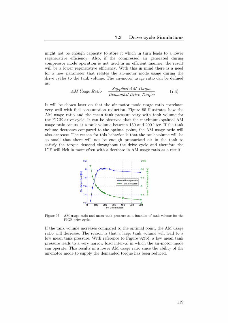
7.3 Drive cycle Simulations
119
might not be enough capacity to store it which in turn leads to a lower regenerative efficiency. Also, if the compressed air generated during compressor mode operation is not used in an efficient manner, the result will be a lower regenerative efficiency. With this in mind there is a need for a new parameter that relates the air-motor mode usage during the drive cycles to the tank volume. The air-motor usage ratio can be defined as:
Supplied AM TorqueAM Usage Ratio = Demanded Drive Torque
(7.4)
It will be shown later on that the air-motor mode usage ratio correlates very well with fuel consumption reduction. Figure 95 illustrates how the AM usage ratio and the mean tank pressure vary with tank volume for the FIGE drive cycle. It can be observed that the maximum/optimal AM usage ratio occurs at a tank volume between 150 and 200 liter. If the tank volume decreases compared to the optimal point, the AM usage ratio will also decrease. The reason for this behavior is that the tank volume will be so small that there will not be enough pressurized air in the tank to satisfy the torque demand throughout the drive cycle and therefore the ICE will kick in more often with a decrease in AM usage ratio as a result.
Figure 95 AM usage ratio and mean tank pressure as a function of tank volume for the FIGE drive cycle.
If the tank volume increases compared to the optimal point, the AM usage ratio will decrease. The reason is that a large tank volume will lead to a low mean tank pressure. With reference to Figure 92(b), a low mean tank pressure leads to a very narrow load interval in which the air-motor mode can operate. This results in a lower AM usage ratio since the ability of the air-motor mode to supply the demanded torque has been reduced.
0 100 200 300 400 500 6007.2
7.4
7.6
7.8
8
8.2
AM
Usa
ge
Ra
tio[%
]
Tank Volume [liter]
0 100 200 300 400 500 6008
8.5
9
9.5
10
10.5
Me
an
Ta
nk
Pre
ssu
re [b
ar]
AM usage ratioTank Pressure

7 Results
120
7.3.3 Determining Minimum Tank Pressure
The minimum allowable tank pressure is an important parameter due to several reasons. In this section it will be shown that the minimum tank pressure has a significant effect on fuel consumption. In Figure 96(a) the regenerative efficiency and fuel consumption as a function of minimum tank pressure can be seen. It can be observed that there exists a minimum tank pressure where fuel consumption is at a minimum while the corresponding regenerative efficiency is at a maximum, in this case for a minimum tank pressure of about 8 bar. The reason why fuel consumption varies with minimum tank pressure can be explained with reference to Figure 96(b), where the mean tank pressure and friction brake usage as a function of minimum tank pressure can be seen. The friction brake usage is defined as the ratio between the amount of brake energy generated by the friction brakes and the total brake energy demanded by the drive cycle. It can be seen that mean tank pressure and friction brake usage increases with minimum tank pressure. The reason for this behavior is the shape of the compressor mode performance map shown in Figure 92(a). For instance, a high mean tank pressure means that the load interval in which the compressor mode can operate and generate brake power is very wide and consequently the friction brake usage during these conditions can be minimized. In Figure 96(a) it can be seen that the fuel consumption initially also decreases until a minimum tank pressure of 8 bar after which it starts to increase. This behavior is closely related to the shape of the performance maps displayed in Figure 92. By moving away from the optimal point at a minimum tank pressure of 8 bar, the operating points will be located in a less favorable area of the performance maps and thus the regenerative efficiency will decrease. A decrease in regenerative efficiency means that there will be less energy available for
(a) (b) Figure 96 Illustration of the effect of minimum tank pressure on various parameters
during the Braunschweig drive cycle; (a) Regenerative efficiency and fuel consumption, (b) Friction brake usage and mean tank pressure.
0 4 8 1214
16
18
20
Re
ge
ne
rativ
e E
ffici
en
cy [%
]
Minimum Tank Pressure [bar]
0 4 8 122.9
3
3.1
3.2
Fu
el C
on
sum
ptio
n [l
/10
km
]
R.EffFC
0 4 8 12 160
15
30
45
60
Fric
tion
Bra
ke U
sag
e [%
]
Minimum Tank Pressure [bar]
0 4 8 12 162
6
10
14
18
Me
an
Ta
nk
Pre
ssu
re [b
ar]
EnergyTankPressure

7.3 Drive cycle Simulations
121
propulsion of the vehicle and therefore the ICE engine has to deliver extra energy to recover the deficit of propulsion energy which results in a direct increase in fuel consumption.
Another aspect that needs attention is the importance of minimum tank pressure when considering the supercharging capabilities of the pneumatic hybrid engine. By setting the minimum tank pressure at a high pressure level, the probability for having access to enough compressed air for supercharging the engine increases. According to [110], the supercharging capability of the pneumatic hybrid engine is very important considering fuel consumption reduction, especially for heavily downsized turbo engines suffering from turbo-lag. Therefore, it is of great importance to keep the supercharging capability of the pneumatic hybrid engine as high as possible. However, the results presented in this sub-section do not take this into account since the air-power assist mode was not implemented in the vehicle model.
7.3.4 Drive Cycle Simulation Results
In this sub-section, the most relevant results from 10 different drive cycles are presented. Figure 97 shows how the tank pressure varies during the FIGE and the New York bus drive cycle. The New York bus drive cycle is characterized by a high rate of stops/km and frequent idling, which in Figure 97(b) is illustrated by constant pressure after a preceding increase in tank pressure. The FIGE drive cycle consists of three parts, including city, rural and motorway driving. The city driving part of the FIGE drive cycle shows similar patterns of frequent change in tank pressure as seen during the New York bus drive cycle. During the rural driving section, the change in tank pressure becomes less frequent and during the last part,
(a) (b) Figure 97 Tank pressure for two different drive cycles; (a) FIGE drive cycle, (b) New
York Bus drive cycle.
0 500 1000 15008
10
12
14
16
18
Time [s]
Ta
nk
Pre
ssu
re [b
ar]
0 100 200 300 400 500 6008
10
12
14
16
18
Time [s]
Ta
nk
Pre
ssu
re [b
ar]

7 Results
122
motorway driving, there is almost no charging of the pressure tank. During motorway driving, the vehicle is propelled at almost constant speed with almost no braking and thus no compressed air will be generated.
An overview of the most important results from the drive cycle simulations can be seen in Table 12. The most important row in Table 12 is the “FC reduction, RB+SS” (fuel consumption reduction with regenerative braking and stop/start functionality) which is a direct measure of the pneumatic hybrid performance. It can be seen that the highest fuel consumption reduction is achieved with the New York bus drive cycle (58.8%) while the FIGE drive cycle has the lowest fuel consumption reduction (8.0%). The mean fuel consumption reduction for all drive cycles combined is about 30%. The reason why there is a considerable difference in fuel consumption reduction between the drive cycles is explained below.
Table 12 Overview of the most relevant results from the drive cycle simulation study for the pneumatic hybrid bus; RB – Regenerative Braking, S/S – Stop/Start.
Drive Cycle CBD NY Bus
NY Comp.
Manh. Bus
O.C. Bus
Braun-schweig FIGE CSC Japan
JE05 HD-
UDDS
Tank Volume [liter]
60 100 110 140 150 160 170 260 260 570
Regen. Efficiency
[%] 14.3 27.7 32.8 21.3 19.4 18.5 28.3 21.7 29.0 23.2
FC, conventional [l/100 km]
39.5 82.6 44.2 60.3 42.8 41.7 25.1 37.2 31.7 32.8
FC, RB +SS [l/100
km] 33.3 34.0 25.7 36.0 30.3 30.1 23.1 25.8 23.0 24.6
FC reduction, RB+SS [%]
15.7 58.8 41.9 40.3 29.2 27.8 8.0 30.6 27.4 25.0
FC, RB only [l/100
km] 37.0 75.5 39.1 54.1 38.6 38.2 24.2 33.8 29.2 30.8
FC reduction RB [%]
6.3 8.6 11.5 10.3 9.7 8.5 3.4 9.2 7.7 6.2
Friction Brake
Usage [%] 27.5 4.9 0.9 8.0 10.7 13.0 22.4 0.3 1.0 8.3

7.3 Drive cycle Simulations
123
The optimal tank volume varies to a great extent with the choice of drive cycle. The CBD drive cycle shows the smallest tank volume (60 liter) while the tank volume for the HD-UDDS is the largest (570 liter). This difference in tank volume between the cycles arises due to the different characteristics of the drive cycles used. The CBD drive cycle shows the highest mean acceleration of all drive cycles while its maximum speed is the lowest, see Figure 31 and Figure 32. This means that the drive load will be very high due to the high acceleration. However, since the maximum speed is low, the acceleration periods are short which means that the air requirement is low which implies that a small tank is adequate. The UDDS drive cycle has a moderate mean acceleration which results in a low maximum drive load compared to more aggressive drive cycles. However, its mean speed is the highest among all cycles, which together with the moderate acceleration results in long acceleration periods and the consequently the air requirement is large which can only be achieved with a large tank.
Figure 98 (a) gives a clearer view of the total fuel consumption reduction and the part of the fuel consumption reduction gained from regenerative braking. By observing the results in Figure 98(a) it can clearly be concluded that the regenerative braking can be accredited for a minor part of the reduction in fuel consumption. Most of the fuel consumption reduction is gained from the stop/start functionality, i.e. elimination of the idle period. Another thing that can be observed in Figure 98(a), is that the New York Bus drive cycle displays the lowest fuel consumption reduction due to regenerative braking in relation to the total fuel consumption reduction. The reason is that the New York bus cycle has the highest rate of idle (65.5%) together with the longest idle periods of all drive cycles examined. A long idle period leads to much larger reduction in fuel consumption compared to what the accompanying pneumatic hybrid operation (compressor mode before and air-motor mode after the idle period) can achieve.
Figure 98(b) illustrates how air-motor mode usage ratio varies with different drive cycles. There is a great resemblance between Figure 98(a) and Figure 98(b), which implies that air-motor mode usage ratio and fuel consumption reduction are strongly related. The relation is illustrated in Figure 99(a) where it can clearly be seen that the fuel consumption reduction is an almost linear function of air-motor mode usage ratio. A high air-motor mode usage ratio means that the amount of time the ICE has to kick in to satisfy the power demand decreases. Figure 99(b) shows how the air-motor mode usage ratio is related to the average speed. A drive cycle with high average speed contains fewer stops/km compared to a drive cycle with lower average speed. A small number of stops/km

7 Results
124
(a) (b)
Figure 98 (a) Fuel consumption reduction achieved with and without (w/o) regenerative braking for the different drive cycles, (b) Air-motor mode usage ratio for the different drive cycles.
(a) (b)Figure 99 (a) Fuel consumption reduction as a function of air-motor mode usage ratio
for the different drive cycles, (b) Air-motor mode usage ratio as a function of average speed for the different drive cycles.
means that the amount of time the engine spends in air-motor mode during the drive cycle will be small and thus the air-motor mode usage ratio will be low, as can be seen in Figure 99(b).
Another thing that can be observed in Table 12 and needs attention is the fact that the regenerative efficiency for the FIGE drive cycle is the third largest of all investigated drive cycles (28.3%) and at the same time it displays the lowest fuel consumption reduction due to regenerative braking (3.4%). The reason is that the regenerative efficiency only gives information about how efficient the recovery of brake energy is, not how long the pneumatic modes will be active. In this case, the friction brake usage parameter and the air-motor mode usage ratio are much better indicators. In the FIGE case, the friction brake usage is the second largest of all investigated drive cycles (22.4%) which indicates that the engine is
0
10
20
30
40
50
60
Fu
el C
on
sum
ptio
n R
ed
uct
ion
[%]
CBD
NYbus
NYcom
p
Man
h
OCbus
BraunS
FIGE
CSCJE
05
UDDS
FC reduction due to S/SFC reduction due to RB
0
10
20
30
40
50
AM
usa
ge
rati
o [
%]
CBD
NYbus
NYcom
p
Man
h
OCbus
BraunS
FIGE
CSCJE
05
UDDS
0 10 20 30 40 50 600
10
20
30
40
50
60
AM usage ratio [%]
Fu
el C
on
sum
ptio
n R
ed
uct
ion
[%]
MeasurmentLinear fit
R2=0.9337
0 10 20 30 40 50 600
10
20
30
40
50
AM
usa
ge
ra
tio [%
]
Average Speed [km/h]
MeasurmentLinear fit
R2=0.7162
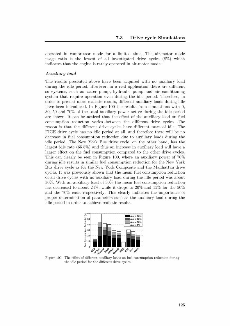
7.3 Drive cycle Simulations
125
operated in compressor mode for a limited time. The air-motor mode usage ratio is the lowest of all investigated drive cycles (8%) which indicates that the engine is rarely operated in air-motor mode.
Auxiliary load
The results presented above have been acquired with no auxiliary load during the idle period. However, in a real application there are different subsystems, such as water pump, hydraulic pump and air conditioning system that require operation even during the idle period. Therefore, in order to present more realistic results, different auxiliary loads during idle have been introduced. In Figure 100 the results from simulations with 0, 30, 50 and 70% of the total auxiliary power active during the idle period are shown. It can be noticed that the effect of the auxiliary load on fuel consumption reduction varies between the different drive cycles. The reason is that the different drive cycles have different rates of idle. The FIGE drive cycle has no idle period at all, and therefore there will be no decrease in fuel consumption reduction due to auxiliary loads during the idle period. The New York Bus drive cycle, on the other hand, has the largest idle rate (65.5%) and thus an increase in auxiliary load will have a larger effect on the fuel consumption compared to the other drive cycles. This can clearly be seen in Figure 100, where an auxiliary power of 70% during idle results in similar fuel consumption reduction for the New York Bus drive cycle as for the New York Composite and the Manhattan drive cycles. It was previously shown that the mean fuel consumption reduction of all drive cycles with no auxiliary load during the idle period was about 30%. With an auxiliary load of 30% the mean fuel consumption reduction has decreased to about 24%, while it drops to 20% and 15% for the 50% and the 70% case, respectively. This clearly indicates the importance of proper determination of parameters such as the auxiliary load during the idle period in order to achieve realistic results.
Figure 100 The effect of different auxiliary loads on fuel consumption reduction during
the idle period for the different drive cycles.
0
10
20
30
40
50
60
Fu
el C
on
sum
ptio
n R
ed
uct
ion
[%]
CBD
NYbus
NYcom
p
Man
h
OCbus
BraunS
FIGE
CSCJE
05
UDDS
Aux = 70%Aux = 50%Aux = 30%Aux = 0%

7 Results
126
7.4 Regenerative Efficiency
In Section 3.4, the regenerative efficiency was defined as the ratio between the energy recovered during air motor operation and the energy consumed during compressor mode operation. In Table 13, the regenerative efficiency calculated from experimental engine data can be seen. The 16 mm tank valve setup has a maximum regenerative efficiency of 33% at 900 rpm. The reason why the efficiency is higher at 900 rpm than at 600 rpm is that the theoretically calculated valve timings by coincidence are better suited at 900 rpm. The regenerative efficiency for the 28 mm tank valve setup indicates that with optimized tank valve timing, the maximum efficiency occurs at 600 rpm and decreases with increasing engine speed. A considerable improvement has been achieved when switching from a 16 mm to a 28 mm tank valve setup. The improvement depends mainly on a large tank valve diameter and optimized tank valve timing during AM. A change in inlet valve strategy from constant IVC to open-loop controlled IVC, contributes to a further increase in regenerative efficiency.
The pneumatic tank valve actuator consumes energy in the form of pressurized air from the pressure tank. Since its energy consumption
Table 13 Regenerative efficiency calculated from experimental engine data for different tank valve setups and valve strategies at three different engine speeds.
ηregen
Engine speed 600 900 1200
16 mm tank valve setup, theoretical valve timings 32 33 25
28 mm tank valve setup, constant IVC during air motor mode, optimized tank valve timings 44 40 37
28 mm tank valve setup, optimized valve timings 48 44 40
decreases the total energy stored in the pressure tank, it has to be considered as an energy loss. These losses have indirectly been taken into account in the calculation of regenerative. This is only valid for the 28 mm valve setup, since the pneumatic tank valve used in the 16 mm valve setup has been fed with compressed air from an eternal source. This means that the regenerative efficiency calculated for the 28 mm large tank valve setup, is lower than it would be if the pneumatic valve actuator pressure consumption was excluded from the calculation.

7.4 Regenerative Efficiency
127
The issue with the tank valve spring explained previously, lead to a premature TankVO, which has also affected the regenerative efficiency negatively. With a valve actuating system capable at opening against high cylinder pressure, further increases in regenerative efficiency can be expected.
During the drive cycle simulations, a considerable variation in regenerative efficiency between the different drive cycles was shown. The highest regenerative efficiency (32.8%) was achieved with the New York Composite drive cycle and the corresponding fuel consumption reduction due to regenerative braking was 11.5%. The lowest regenerative efficiency (14.3%) was observed for the CBD drive cycle and the corresponding fuel consumption reduction due to regenerative braking was 6.3%. There was no clear correlation between regenerative efficiency and the reduction in fuel consumption due to regenerative braking. The second largest fuel consumption reduction attributed to regenerative braking (10.3%) was achieved with one of the lowest regenerative efficiency.

128
Chapter 8
8 Summary
The work presented in this thesis is of both experimental and theoretical nature with the aim to illustrate the potential with pneumatic hybridization of vehicles.
Pneumatic hybridization is a promising concept with the possibility to reduce vehicle fuel consumption as well as exhaust emissions. The advantages with pneumatic hybrid compared to the electric hybrid are first and foremost simplicity combined with a great potential for cost reduction. Initial testing of different pneumatic hybrid engine modes of operation was conducted. Both compressor mode (CM) and air-motor mode (AM) were executed successfully and a regenerative efficiency of up to 33 % was achieved showing the potential with pneumatic hybridization.
In order to minimize pressure losses due to restricted flow into and out from the cylinder, the tank valve head diameter was changed from 16 mm to 28 mm. The large tank valve was combined with an in-house developed pneumatic spring in order to secure proper valve timing. The evaluation showed that there are some issues with the pneumatic valve spring concerning tank valve actuation. A method for optimizing both CM and AM in terms of efficiency was developed and tested. The results indicate an increase in efficiency for both CM and AM. The impact of optimized valve timings was much more evident in AM compared to CM. Optimized pneumatic hybrid operation together with the change of valve head geometry showed an increase in regenerative efficiency from 33% to impressive 48%. However, this figure includes energy losses due to pressure tank fed valve actuation. Therefore, the increase in indicated efficiency is expected to be even higher.
It was further identified that an important aspect of the compressor mode is its ability to control the amount of braking power. Therefore, a control strategy for load control during compressor mode operation was developed and investigated. The proposed controller, which consists of a feedforward controller based on experimental data and a PID controller, performed satisfactorily with regards to set-point tracking and disturbance rejection.

8 Summary
129
A model of the pneumatic hybrid engine was developed in the engine simulation package GT-Power and validated against experimental data. After a successful validation process, the model was used for parameterization purposes. In this way the influence of important parameters such as tank valve diameter, tank valve opening and closing could, together with their effect on pneumatic hybrid engine performance, be investigated.
A pneumatic hybrid vehicle model was developed and evaluated over ten different drive cycles. The simulations showed that fuel consumption varies heavily with the choice of drive cycles. The New York bus drive cycle shows a fuel consumption reduction of up to 58% for the pneumatic hybrid vehicle while the FIGE drive cycle only shows a modest fuel consumption reduction of about 8%. It has been shown that regenerative braking only accounts for up to about 12% of this fuel consumption reduction at best. The remaining part of the fuel consumption reduction is mainly due to the stop/start functionality. The main reason why fuel consumption varies with different drive cycles is their driving patterns. Average fuel consumption highly depends on parameters such as acceleration, deceleration, average speed and number of stops/km. The results indicate that drive cycles based on city driving that are not aggressive with low average speed and low number of stops benefit from pneumatic hybrid operation. For drive cycles that predominantly are high-speed cycles and involve very few stops, the pneumatic hybrid will have a modest influence on the reduction in fuel consumption.

130
Chapter 9
9 Discussion
During the last decade, the popularity of hybrid vehicles has increased almost exponentially and will most probably continue to do so for the coming decade, at least until the breakthrough of battery electric vehicles (if there will be any). With proper conditions, there is a possibility that the pneumatic hybrid vehicle will see the light of day during this period. However, for this to happen, the introduction of a commercial camless VVA system on the market is needed together with the willingness of major vehicle manufacturers to consider it as a worthy alternative to their already in-production hybrid electric vehicle.
The intent with this thesis is to show the potential of the PHV together with the hurdles/obstacles that needs to be overcome. For this purpose both experimental and theoretical work has been conducted. The reference value of the work presented in this thesis is of great importance for future research in this interesting field since it to a great extent, gives a clear picture of the concept and the factors affecting it.
The first couple of papers presented in this thesis, dealt with fundamental pneumatic hybrid operation demonstrated successfully by experiments. The influence of parameters such as valve diameter and valve timings on pneumatic hybrid operation was presented. However, due to two main reasons it was realized that there is a need for an engine model to fully understand the underlying phenomena affecting the pneumatic hybrid engine performance. One of the reasons was, that it proved to be rather time consuming to change physical parameters such as valve diameter. The second reason was issues with the pneumatic spring used in the tank valve arrangement. At some conditions, a proper functionality could not be secured due to unknown defects in the proposed pneumatic spring solution. Unfortunately, this issue affects the results in a negative manner and gives a false picture of the underlying phenomena affecting the pneumatic hybrid operation. These two reasons motivated the development of an engine model where the issues of faulty valve operation together with the waste of time associated with change of physical parameters, can be completely avoided.

9 Discussion
131
The experimental engines used during the studies presented in this thesis were single-cylinder engines which lack the dynamics associated with a multi-cylinder engine, which in turn leaves its mark on the results. With a multi-cylinder engine it would have been possible to run the engine according to a drive cycle on a dynamometer in order to estimate the fuel consumption of a vehicle equipped with a pneumatic hybrid powertrain. This motivated the development of a vehicle model. The intent with the vehicle model simulation was primarily to demonstrate the potential of the PHV, not to give as exact a prediction as possible. If the primary goal would be to develop a model as accurate as possible, a lot more work would have to be invested. For instance, the auxiliary demand during the drive cycles examined is only estimated for the Braunschweig drive cycle and then applied for all drive cycles. The auxiliary demand will vary heavily over a certain drive cycle and between different drive cycles. This indicates that for maximum accuracy of the fuel consumption estimation, all auxiliary units needs to be accurately modeled. However, since the pneumatic hybrid vehicle is compared to a corresponding conventional vehicle modeled in the same environment, the difference in fuel consumption between these two models should be a good guideline for real life fuel consumption reduction. The fuel consumption reduction for some drive cycles was very high (58%) which might be a little too optimistic. However, by averaging the fuel consumption reduction for all investigated drive cycles, a fuel consumption reduction of 30% is obtained which seems to be reasonable.
The most prominent performance indicator associated with the PHV, besides fuel consumption, is the regenerative efficiency. During the experimental studies presented in this thesis it was established that a regenerative efficiency as high as possible is to be preferred. However, the simulation studies showed that, with regards to fuel consumption reduction, a high regenerative efficiency is not always necessary. It should be noticed that at very low loads a high regenerative efficiency can be achieved, but the gain in fuel consumption reduction will be minimal. On the other hand a high, braking load during compressor mode operation will lead to a low regenerative efficiency while the fuel consumption reduction would still be at a level comparable to at a case with lower braking load.

132
Chapter 10
10 Future Work
So far, the experimental work described in this thesis was conducted on a single-cylinder engine. The next natural step would be to convert a multi-cylinder engine to work an as pneumatic hybrid engine. In this way the effects of the dynamics, associated with multi-cylinder engines, on pneumatic hybrid operation can be investigated. A multi-cylinder engine allows the possibility to run the engine according to different drive cycles in order to estimate the fuel consumption in a more realistic way compared to models. The author of this thesis has also conducted some initial experiments regarding the supercharging capability of the pneumatic hybrid engine. However, due to strict deadline no time for evaluation of this data was available. In the future these data needs to be evaluated in order to understand this mode better and to investigate it more thoroughly.
In this thesis a study focused on load control during compressor mode operation was presented. The same needs to be done with regards to air-motor and air-power assist operation.
The effects of the different engine modes on exhaust emissions have completely been omitted in this thesis and needs to be investigated in the future.
The pneumatic valve spring used in the project summarized in this thesis needs some further development in order to eliminate all discovered issues that affect the performance of the pneumatic hybrid engine negatively.
The vehicle model needs further development in order to predict the performance parameters as accurate as possible. The pneumatic hybrid engine model needs more advanced control for operation of the different engine modes. Also, in present engine model the APAM is not included and therefore its eventual effect on fuel consumption was not investigated. This is something that needs to be addressed in the future development of the vehicle model. Vehicle sub-models such as all auxiliaries needs more development in order to more accurately simulate realistic behavior.

10 Future Work
133
The ultimate goal of future projects will be the development of an experimental prototype vehicle. With such a vehicle, the true potential of the pneumatic hybrid concept can be proven.
134
Chapter 11
11 References
1. European Parliament, “Beating global climate change”, (2005). Available at www.europarl.eu.int (Dec 12, 2010)
2. European Parliament, ”Emission performance standards for new passenger cars ***I”, (2008). Available at: www.europarl.europa.eu (Dec. 1, 2010)
3. G. Fontaras, P. Pistikopoulos and Z. Samaras, ”Experimental evaluation of hybrid vehicle fuel economy and pollutant emissions over real-world simulation driving cycles”, Atmospheric Environment 42, pp. 4023-4035, 2008.
4. A. Folkesson, C. Andersson, P. Alvfors, M. Alaküla and L. Overgaard, ”Real life testing of a Hybrid PEM Fuel Cell Bus”, J. of Power Sources 118, pp 349-357, 2003.
5. G. Foyt, “Demonstration and Evaluation of Hybrid Diesel-Electric Transit Buses – Final Report”, Connecticut Academy of Science and Engineering R, CT-170-1884-F-05-10, 2005.
6. M. Schechter, “Regenerative Compression Braking – a Low Cost Alternative to Electric Hybrids”, SAE Technical Paper 2000-01-1025, 2000.
7. C. Tai, T-C Tsao, M. Levin, G. Barta and M. Schechter, “Using Camless Valvetrain for Air Hybrid Optimization”, SAE Technical Paper 2003-01-0038, 2003.
8. I. Vasile. P. Higelin, A. Charlet and Y. Chamaillard, “Downsized engine torque lag compensation by pneumatic hybridization”, 13th International Conference on Fluid Flow Technologies, 2006.
9. C. Dönitz, I. Vasile, C. Onder and L. Guzzella, “Realizing a Concept for high Efficiency and Excellent Drivability: The

11 References
135
Downsized and Supercharged Hybrid Pneumatic Engine”, SAE Techincal Paper 2009-01-1326, 2009.
10. M. Andersson, B. Johansson and A. Hultqvist, “An Air Hybrid for High Power Absorption and Discharge”, SAE Technical Paper 2005-01-2137, 2005.
11. S. Trajkovic, P. Tunestål and B. Johansson, “Investigation of Different Valve Geometries and Valve Timing Strategies and their Effect on Regenerative Efficiency for a Pneumatic Hybrid with Variable Valve Actuation”, SAE Technical Paper 2008-01-1715, 2008.
12. S. Trajkovic, P. Tunestål and B. Johansson, “A Simulation Study Quantifying the Effects of Drive Cycle Characteristics on the Performance of a Pneumatic Hybrid Bus”, ASME Technical Paper ICEF2010-35093, 2010.
13. Toyota Motor Corporation, “Worldwide Sales of TMC Hybrids Top 2 Million Units”, Press Release, September 4, 2009.
14. V. Reding, “Regulation (EC) No 717/2007 of the European Parliament and of the Council”, Official Journal of the European union, June 29 2007, p.4
15. L. Gaedt, D. Kok, F. Goodfellow, D. Tonkin, C. Picod and M. Neu, “HyTrans – A micro-hybrid Transit from Ford”, ICAT 2004, Istanbul, Turkey, 2004
16. A.F. Burke, “Saving Petroleum with Cost-Effective Hybrids, SAE Technical Paper 2003-01-3279, 2003
17. M. Samulski and C. Jackson, “Effects of Steady-State and Transient Operation on Exhaust Emissions from Nonroad and Highway Diesel Engines”, SAE Technical Paper 982044, 1998
18. Toyota, “Toyota Prius – 2008 Performance and Specifications”. Available at http://www.toyota.com/prius-hybrid/specs.html, (Dec 6, 2010)
19. J. Ottoson, “Energy Management and Control of Electrical Drives in Hybrid Electrical Vehicles”, Licenciate thesis, Department of Industrial Electrical Engineering and Automation, Lund University, Lund, 2006

11 References
136
20. P. Bossche, “The electric vehicle: raising the standards”, PhD Thesis, Vrije Universiteit Brussel, Belgium, 2003
21. M. Ehsani, Y. Gao, S. Gay and A. Emadi, “Modern Electric, Hybrid Electric, and Fuel Cell Vehicles: Fundamentals, Theory, and Design”, CRC Press, 2004
22. E.H. Wakefield, “History of the Electric Automobile: Hybrid Electric Vehicles, Society of Automotive Engineers (SAE), 1998.
23. Anon., “Fuel economy guide”, DOE/EE-0236, US Department of Energy/US Environmental Protection Agency, 2001.
24. L.B. Lave and H.L. MacLean, “An environmental-economic evaluation of hybrid electric vehicles: Toyota’s Prius vs. its conventional internal combustion engine Corolla”, Transportation Research Part D 7 (p 155-162), 2002.
25. Anon., “Fuel economy guide”, DOE/EE-0333, US Department of Energy/US Environmental Protection Agency, 2010.
26. K. Chandler, K. Walkowicz and L. Eudy, “New York City Transit Diesel Hybrid-Electric Buses: Final Results”, DOE/NREL Transit Bus Evaluation Project, NREL/BR-540-32427, 2002
27. P.K. Chiang, “Two-Mode Urban Transit Hybrid Bus In-Use Fuel Economy Results from 20 Million Fleet Miles”, SAE Technical paper 2007-01-0272, 2007
28. Z. Filipi and Y.J. Kim, “Hydraulic Hybrid Propulsion for Heavy Vehicles: Combining the Simulation and Engine-In-the-Loop Techniques to Maximize the Fuel Economy and Emission Benefits” Oil & Gas Science and Technology – Rev. IFP, Vol. 65, No. 1, pp. 155-178, 2010
29. L.Guzzella and A. Sciarretta “Vehicle Propulsion Systems - Introduction to Modeling and Optimization”, 2nd editon, Springer, 2007.
30. J.D. Van de Ven, M.W. Olson, and P.Y. Li, “Development of a hydro-mechanical hydraulic hybrid drive train with independent wheel torque control for an urban passenger vehicle”. In Proceedings of the International Fluid Power Exposition, pp. 11–15, 2008.

11 References
137
31. J. Alson, D. Barba, J. Bryson, M. Doorag, D. Haugen, J. Kargul, J. McDonald, K. Newman, L. Platte and M.Wolcott, “Progress Report on clean and Efficient Automotive Technologies under Development at EPA”, EPA420-R-04-002, United States Environmental Protection Agency, 2004
32. R. Johri and Z. Filipi, “Low-Cost Pathway to Ultra Efficient City Car: Series Hydraulic System with Optimized Supervisory Control”, SAE Technical Paper 2009-24-0065, 2009
33. M. Forssén, “Bränslecelldrivna stadsbussar: Förstudie”, KFB, 1999:15, 1999
34. C. Ramos-Paja, C. Bordons, A. Romero, R. Giral and L. Martínez-Salamero, “Minimum Fuel Consumption Strategy for PEM Fuel Cells”, IEEE Trans. Ind. Electron., vol. 56, no. 3, pp. 685-696, March 2009.
35. Honda, ”Specifications: The Honda FCX”, Available at: http://world.honda.com/FuelCell/FCX/specifications/ (Dec. 8 2010)
36. Honda, “FCX Clarity: Honda Debutes All-New FCX Clarity”, Available at: http://world.honda.com/FCXClarity/index.html (Dec. 8 2010)
37. Toyota, “Toyota Develops Advanced Fuel Cell Hybrid Vehicle”, Available at: http://www.toyota.co.jp/en/news/08/0606_2.html (Dec. 8 2010)
38. A. Folkesson, C. Andersson, P. Alvfors, M. Alaküla and L. Overgaard, ”Real life testing of a Hybrid PEM Fuel Cell Bus”, Journal of Power Sources, vol. 118, pp. 349-357, 2003
39. R.K Ahluwalia, X. Wang and A. Rousseau, “Fuel economy of hybrid fuel-cell vehicles”, Journal of Power Sources, vol. 152, pp. 233-244, 2005.
40. D. Cross and C. Brockbank, “Mechanical Hybrid System Comprising a Flywheel and CVT for Motorsport and Mainstream Automotive Applications”, SAE Technical paper 2009-01-1312, 2009.
41. C. Brockbank and C. Greenwood, “Fuel Economy Benefits of a Flywheel & CVT Based Mechanical Hybrid for City Bus and
11 References
138
Commercial Vehicle Applications”, SAE Technical paper 2009-01-2868, 2009.
42. C. Thai, T-C Tsao, M. Levin, G. Barta and M. Schechter, “Using Camless Valvetrain for Air Hybrid Optimization”, SAE Paper 2003-01-0038, 2003
43. M. Andersson, B. Johansson and A. Hultqvist, “An Air Hybrid for High Power Absorption and Discharge”, SAE paper 2005-01-2137, 2005
44. C. Dönitz, I. Vasile, C. Onder and L. Guzzella, “Realizing a Concept for High Efficiency and Excellent Driveability: The Downsized and Supercharged Hybrid Pneumatic Engine”, SAE Technical paper 2009-01-1326, 2009.
45. M. Schechter, “New Cycles for Automobile Engines”, SAE Technical paper 1999-01-0623, 1999.
46. S. Trajkovic, P. Tunestål and B. Johansson, “Introductory Study of Variable Valve Actuation for Pneumatic Hybridization”, SAE Technical Paper 2007-01-0288, 2007
47. S. Trajkovic, P. Tunestål and B. Johansson, “Investigation of Different Valve Geometries and Valve Timing Strategies and their Effect on Regenerative Efficiency for a Pneumatic Hybrid with Variable Valve Actuation”, SAE Technical Paper 2008-01-1715, 2008
48. S. Trajkovic, P. Tunestål and B. Johansson, “A Simulation Study Quantifying the Effects of Drive Cycle Characteristics on the Performance of a Pneumatic Hybrid Bus”, ASME Technical Paper ICEF2010-35093, 2010
49. J. K. Broderick, “Combined internal combustion and compressed air engine”, US Patent 1013528, Jan 1912
50. W. Ochel, O. Beyermann and F. Gehrmann, “Multicylinder 4-stroke cycle diesel engine and compressor”, US Patent 2676752, April 1954
51. R. Brown, ”Compressed air engine”, US Patent 3765180, October 1973
52. T. Ueno, ”Convertible engine-air compressor apparatus for driving a vehicle”, US Patent 3963379, June 1976

11 References
139
53. D.F Moyer, “Hybrid Internal Combustion Engine”, US Patent 5695430, December 1997.
54. T. Glad and L. Ljung, ”Reglerteknik – Grundläggande teori”, Studentlitterature, Sweden, 2008.
55. Y.A. Cengel and M.A Boles, “Thermodynamics an Engineering Approach”, 4th ed., McGraw-Hill, 2002.
56. C. Psanis, “Modelling and Experimentation on Air Hybrid Engine Concepts for Automotive Applications”, PhD Thesis, School of Engineering, Brunel University, West London, United Kingdom, 2007.
57. C. Dönitz, I. Vasile, C.H. Onder and L Guzzella, “Modelling and optimizing two- and four-stroke hybrid pneumatic engines”, Proc. IMechE Vol. 223 Part D: J. Automobile Engineering, pp. 255-280, 2009
58. C.Y. Lee, H. Zhao and T. Ma, “A Low Cost Air Hybrid Concept”, Oil & Gas Science and Technology - Rev. IFP, Vol. 65, No. 1, pp. 19-29, 2010.
59. G. Garcea, “Timing variator for the timing system of a reciprocating internal combustion engine”, US Patent 4231330, November 1980
60. B. Johansson, “Förbränningsmotorer del 2”, 2004
61. H. Heisler, “Advanced Engine Technology”, SAE International, Warrendale, PA, 1995
62. M. Grohn, “The New Camshaft Adjustment System by Mercedes-Benz – Design and Application in 4-Valve Engines”, SAE Technical Paper 901727, 1990
63. Y. Moriya, A. Watanabe, H. Uda, H. Kawamura and M. Yoshioka, “A Newly Developed Intelligent Variable Valve Timing System – Continuously Controlled Cam Phasing as Applied to a New 3 Liter Inline 6 Engine”, SAE Technical Paper 960579, 1996
64. K. Inoue, K. Nagahiro, Y. Ajiki and N. Kishi, “A High Power, Wide Torque Range, Efficient Engine with a Newly Developed Variable-Valve-Lift and -Timing Mechanism”, SAE Technical Paper 890675,1989

11 References
140
65. K. Hatano, K. Lida, H. Higashi, and S. Murata, “Development of a New Multi-Mode Variable Valve Timing Engine”, SAE Technical Paper 930878, 1993
66. C. Brüstle and D. Schwarzenthal, “The “Two-in-One” Engine – Porsche’s Variable System (VVS)”, SAE Technical Paper 980766, 1998
67. C. Brüstle and D. Schwarzenthal, “VarioCam Plus – A highlight of the Porsche 911 Turbo Engine”, SAE Technical Paper 2001-01-0245, 2001
68. S. Birch, “Porsche Developments”, Automotive Engineering International, July 2000
69. T. Shikida, Y. Nakamura, T. Nakakubo and H. Kawase, ”Development of the High Speed 2ZZ-GE Engine”, SAE Technical Paper 2000-01-0671
70. R.Flierl and M. Klüting, “The third Generation of Valvetrains – new Fully Variable Valvetrains for Throttle-Free Load Control”, SAE Technical Paper 2000-01-1227, 2000
71. J. Edgar, “BMW's Valvetronic! The first petrol engine without a throttle butterfly?”, Autospeed, issue 144, August 2001. Available at http://www.autospeed.com/cms/A_1083/article.html, (Dec. 4, 2010)
72. A. Titolo, “The Variable Valve Timing System – Application on a V8 Engine”, SAE Technical Paper 910009, 1991
73. B. Lequesne, “Bistable electromechanical valve actuator”, US Patent 4779582, October 1988
74. M. Theobald, B. Lequesne and R. Henry, “Control of Engine Load via Electromagnetic Valve Actuators”, SAE Technical Paper 940816, 1994
75. D. Cope, A. Wright, C. Corcoran, K. Pasch and D. Fischer, “Fully Flexible Electromagnetic Valve Actuator: Design, Modeling and Measurement”, SAE Technical Paper 2008-01-1350, 2008
76. L. Mianzo, B. Collins, I. Haskara and V. Kokotovic, “Electromagnetic valve actuator with soft-seating”, US Patent 6817592, November 2004

11 References
141
77. M. Schechter and M. Levin, “Camless Engine”, SAE Technical Paper 960581, 1996
78. J. Allen and D. Law, “Production Elector-Hydraulic Variable Valve-Train for a New Generation of I.C. Engines”, SAE Technical Paper 2002-01-1109, 2002
79. J. Allen and Don law, “Advanced Combustion Using a Lotus Active Valve Train. Internal Exhaust Gas Recirculation Promoted Auto Ignition”, IFP International Congress, 2001
80. N. Milovanovic, J. Turner, S Kenchington, G. Pitcher and D. Blundell, “Active valvetrain for homogeneous charge compression ignition”, International Journal of Engine Research, Volume 6, Number 4, July 2005
81. J. Turner, S Kenchington and D. Stretch, “Production AVT development: Lotus and Eaton’s Electrohydarulic Closed-Loop Fully Variable Valve Train System”, 25th International Vienna Motor Symposium, 2004
82. Cargine Engineering AB,” Free Valve Technology”. Available at http://www.cargine.com/tech2.html, (Dec. 4, 2010)
83. S. Trajkovic, A. Milosavljevic, P. Tunestål, B. Johansson, ”FPGA Controlled Pneumatic Variable Valve Actuation”, SAE Paper 2006-01-0041, 2006
84. J. Ma, H. Schock, U. Carlson, A. Höglund and M. Hedman, “Analysis and Modeling of an Electronically Controlled Pneumatic Hydraulic Valve for an Automotive Engine”, SAE Technical Paper 2006-01-0042, 2006
85. D.E. Johnson and D.S Johnson, ”Engine with pneumatic valve actuation”, US Patent 4702147, October 1987
86. W. Richeson and F. Erickson, “Pneumatic actuator with permanent magnet control valve latching”, US Patent 4852528, August 1989
87. L. Gould, W. Richeson and F. Erickson, “Performance Evaluation of a Camless Engine Using Valve Actuators with Programmable Timing”, SAE Technical Paper 910450, 1991
11 References
142
88. J. Watson and R. Wakeman, “Simulation of a Pneumatic Valve Actuation System for Internal Combustion Engine”, SAE Technical Paper 2005-01-0771, 2005
89. J. Willand, R. Nieberding, G. Vent and C. Enderle, “The Knocking Syndrome – Its Cures and Its Potential”, SAE Technical Paper 982483, 1998
90. G. Kontarakis, N. Collings and T. Ma, “Demonstration of HCCI Using a Single Cylinder Four-stroke SI Engine with Modified Valve Timing”, SAE Technical Paper 2000-01-2870, 2000
91. O. Lang, W. Salber, J. Hahn, S. Pischinger, K. Hortmann and C. Brüker, ”Thermodynamical and Mechanical Approach Towards a Variable Valve Train for the Controlled Auto Ignition Combustion Process”, SAE Technical Paper 2005-01-0762, 2005
92. N. Kaahaaina, A. Simon, P. Caton and C. Edwards, “Use of Dynamic Valving to Achieve Residual-Affected Combustion”, SAE Technical Paper 2001-01-0549, 2001
93. D. Law, D. Kemp, J. Allen, G. Kirkpatrick and T. Copland, “Controlled Combustion in a IC-Engine with a Fully Variable Valve Train”, SAE Technical Paper 2001-01-0251, 2001
94. L. Cummins, “Internal Fire”, Carnot Press, 2000
95. R. Miller, “High-pressure supercharging system”, US Patent 2670595, March 1954
96. D. Luria, Y. Taitel and A. Stotter, “The Otto-Atkinson Engine – A new Concept in Automotive Economy”, SAE Technical Paper 820352, 1982
97. Toyota, “The heart and soul of hybrid synergy drive”. Available at http://www.toyota.com/html/hybridsynergyview/2004/october/heartandsoul.html, (Dec. 5, 2010)
98. C. Morrissey and T. Shedd, “Experimental Validation of a Carburetor Model in One-Dimensional Engine Software”, SAE Technical Paper 2008-32-0043, 2008
99. F. Westin and H.E. Ångström, “Simulation of a Turbocharged SI-Engine with Two Software and Comparison with Measured Data”, SAE Technical Paper 2003-01-3124, 2003.

11 References
143
100. M. Alaküla, K. Jonasson, C. Andersson, B. Simonsson, S. Marksell, “Hybrid Drive Systems for Vehicles - Part 1”, Department of Industrial Electrical Engineering and Automation, Lund University, 2004. Available at: http://www.iea.lth.se/hfs/Kompendium2006, Last accessed 12 Dec. 2010.
101. K. Svensson, “Variable Compression Ratio for Incresing the Power Density if Heavyduty Diesel Engines”, Master Thesis, Dept. of Energy Sciences, Lund University, Lund, Sweden, 2004.
102. C. Andersson, “On auxiliary systems in commercial vehicles”, Ph.D. Thesis, Dept. of Industrial Electrical Engineering and Automation, Lund University, Lund, Sweden, 2004.
103. DieselNet, “Emission Test Cycles”, Available at: http://www.dieselnet.com/standards/cycles (Dec. 12 2010)
104. D.R. Lancaster, R.B. Kreiger, and J.H. Lienesch, "Measurement and Analysis of Engine pressure Data," SAE Technical Paper 750026, SAE Trans., vol. 84,1975
105. P. Tunestål, “Estimation of the In-Cylinder Air/Fuel Ratio of an Internal Combustion Engine by the Use of Pressure Sensors, 2001
106. S. Trajkovic, P. Tunestål and Bengt Johansson, ”Simulation of a Pneumatic Hybrid Powertrain with VVT in GT-Power and Comparison with Experimental Data”, SAE Technical Paper 2009-01-1223, 2009
107. T.T Tsung and L.L Han, “Evaluation of dynamic performance of pressure sensors using a pressure square-like wave generator”, Measurement Science and Technology 15, pp 1133-1139, 2004
108. J.B Heywood, “Internal Combustion Engine Fundamentals”, McGraw-Hill, Inc, 1988, (s.215)
109. H.D Baumann, “Control Valve Primer: A User’s Guide”, 4th ed., North Carolina: ISA, 2009
110. C. Dönitz, I. Vasile, C. Onder and L. Guzzella, “Realizing a Concept for High Efficiency and Excellent Drivability: The Downsized and Supercharged Hybrid Pneumatic Engine”, SAE Technical Paper 2009-01-1326, 2009
144
Chapter 12
12 Summary of Papers
12.1 Paper I
Introductory Study of Variable Valve Actuation for Pneumatic Hybridization SAE Technical Paper 2007-01-0288 By Sasa Trajkovic, Per Tunestål and Bengt Johansson Presented by Sasa Trajkovic at the SAE World Congress, Detroit, MI, USA, April 2007 In this paper the pneumatic hybrid concept was investigated. A Scania D12 engine was converted for pneumatic hybrid operation and tested in a laboratory setup. Pneumatic valve actuators were used to make the pneumatic hybrid possible. The intent with this paper was to test and evaluate two different modes of engine operation - compression mode (CM) where air is stored in an air tank during deceleration and air-motor mode (AM) where the previously stored air is used for acceleration of the vehicle. This paper also includes optimization of the compressor mode with respect to valve timing.
The results showed that the pneumatic hybrid has a potential in becoming a serious contender to the electric hybrid. The regenerative efficiency was below expected value, but still enough for a proof of concept. It was also realized that the chosen valve geometry was the main limiting parameter regarding regenerative efficiency.
The first author did the experiments, evaluated the data and wrote the paper.

12 Summary of Papers
145
12.2 Paper II
Investigation of Different Valve Geometries and Valve Timing Strategies and their Effect on Regenerative Efficiency for a Pneumatic Hybrid with Variable Valve Actuation SAE Technical Paper 2008-01-1715 By Sasa Trajkovic, Per Tunestål and Bengt Johansson Presented by Sasa Trajkovic at the SAE 2008 International Powertrains, Fuels and Lubricants Congress, Shanghai, China, June 2008 This paper can be seen as a continuation of Paper 2 where it was also realized that the chosen valve geometry was the main limiting parameter with regard to regenerative efficiency. In this paper the tank valve used in Paper 2 has been exchanged for a valve with a larger head diameter in combination with a pneumatic valve spring.
A comparison between the old and the new tank valve geometry and their effect on the pneumatic hybrid efficiency has been done. Also, optimization of the valve timings for both compressor mode and air-motor mode has been done in order to achieve further improvements of regenerative efficiency.
The results indicate that the increase in valve diameter reduces the pressure drop over the tank valve, contributing to a higher regenerative efficiency. Optimization of both tank valve timing and inlet valve timing for CM and AM contributes to a further increase in regenerative efficiency.
The first author did the experiments, evaluated the data and wrote the paper.
12.3 Paper III
Simulation of a Pneumatic Hybrid Powertrain with VVT in GT-Power and Comparison with Experimental Data SAE Technical Paper 2009-01-1323 By Sasa Trajkovic, Per Tunestål and Bengt Johansson Presented by Sasa Trajkovic at the SAE World Congress, Detroit, MI, USA, April 2009 This paper describes a model of the pneumatic hybrid engine, based on a Scania D12 diesel engine. The model was created in GT-Power and it was successfully validated against experimental data from Paper 1 and Paper
12 Summary of Papers
146
2. The paper also included a parametric study in order to give a more in-depth overview on different parameters affecting the pneumatic hybrid performance. The first author developed the model, evaluated the data and wrote the paper.
12.4 Paper IV
Vehicle Driving Cycle Simulation of a Pneumatic Hybrid Bus Based on Experimental Engine Measurements SAE Technical Paper 2010-01-0825 By Sasa Trajkovic, Per Tunestål and Bengt Johansson Presented by Sasa Trajkovic at the SAE World Congress, Detroit, MI, USA, April 2010 In this paper a vehicle model of the pneumatic hybrid was presented. The model was created in Matlab™/Simulink with an engine model based on data obtained with the GT-Power model described in Paper 3. Parameters such as tank volume and minimum allowable tank pressure were investigated. The model was tested over the Braunschweig bus drive cycle and a fuel consumption reduction by almost 30% compared to a conventional vehicle was shown. Regenerative braking account for about 10 percentage points of the reduction in fuel consumption, while the remaining 20 percentage points, can be attributed to stop/start functionality. The first author developed the model, evaluated the data and wrote the paper.
12.5 Paper V
A Simulation Study Quantifying the Effects of Drive Cycle Characteristics on the Performance of a Pneumatic Hybrid Bus ASME Technical Paper ICEF2010-35093 By Sasa Trajkovic, Per Tunestål and Bengt Johansson Presented by Sasa Trajkovic at ASME 2010 Internal Combustion Engine Division Fall Technical Conference, San Antonio, TX, USA, 2010 This paper is a continuation of Paper 4. The pneumatic hybrid vehicle model was investigated over 10 different standard driving cycles. An in-depth analysis of the drive cycle specific characteristics on the pneumatic

12 Summary of Papers
147
hybrid performance is given. The results showed that drive cycle characterized by low aggressively with regards to acceleration and deceleration, low mean speed and large number of stops/km would benefit the most from pneumatic hybridization. The highest fuel consumption reduction (58%) was achieved over the New York drive cycle and the mean fuel consumption reduction for all drive cycles combined was shown to be about 30%. The first author ran the simulations, evaluated the data and wrote the paper.
12.6 Paper VI
A Study on Compression Braking as a Means for Brake Energy Recover for Pneumatic Hybrid Powertrains By Sasa Trajkovic, Per Tunestål and Bengt Johansson To be published in the International Journal of Powertrains 2011 In this paper, a more in-depth look on the different parameters affecting the compressor mode operation was presented. It was shown that parameters such as valve head diameter, TankVO, TankVC and IVO were investigated influence the performance of the compressor mode considerably. It was further recognized that pressure wave propagation affected the mass flow in to and out from the tank considerably. The first author did the experiments, evaluated the data and wrote the paper.
12.7 Paper VII
VVT Aided Load Control during Compressor Mode Operation of a Pneumatic hybrid Powertrain By Sasa Trajkovic, Claes-Göran Zander, Per Tunestål and Bengt Johansson To be submitted to the 2011 JSAE/SAE International Powertrains, Fuel & Lubricants Congress, Kyoto, Japan, 2011
In this paper a control strategy was propose in order to control the load during compressor mode. The proposed controller consists of a feedforward controller based on experimental data and a PID controller. The performance of the controller was investigated by observing the

12 Summary of Papers
148
process respond to different types of changes in set-point together with its ability to reject disturbances. The proposed controller performed satisfactorily with regards to set-point tracking and disturbance rejection, and very low response and settling times where demonstrated.
The first and second author discussed and created a load control strategy, the first author did the experiments, evaluated the data and wrote the paper.

Paper 1

2007-01-0288
Introductory Study of Variable Valve Actuation for Pneumatic Hybridization
Sasa Trajkovic, Per Tunestål and Bengt Johansson Division of Combustion Engines, Lund University, Faculty of Engineering
Urban Carlson and Anders Höglund Cargine Engineering AB
Copyright © 2007 SAE International
ABSTRACT
Urban traffic involves frequent acceleration and deceleration. During deceleration, the energy previously used to accelerate the vehicle is mainly wasted on heat generated by the friction brakes. If this energy that is wasted in traditional IC engines could be saved, the fuel economy would improve. One solution to this is a pneumatic hybrid using variable valve timing to compress air during deceleration and expand air during acceleration. The compressed air can also be utilized to supercharge the engine in order to get higher load in the first few cycles when accelerating.
A Scania D12 single-cylinder diesel engine has been converted for pneumatic hybrid operation and tested in a laboratory setup. Pneumatic valve actuators have been used to make the pneumatic hybrid possible. The actuators have been mounted on top of the cylinder head of the engine. A pressure tank has been connected to one of the inlet ports and one of the inlet valves has been modified to work as a tank valve. The goal has been to test and evaluate 2 different modes – compression mode (CM) where air is stored in an air tank during deceleration and air-motor mode (AM) where the previously stored pressurized air is used for accelerating the vehicle. This paper also includes an optimization of the CM.
INTRODUCTION
As fuel prices increase, together with more stringent pollution standards, the demand for better fuel economy increases. Today there are several solutions to meet this demand and one of them is electric hybrids. In urban traffic the vehicle has to accelerate and decelerate frequently. In conventional vehicles the energy used for acceleration of the vehicle is wasted in the form of heat generated by the friction brakes during deceleration. This leads to a higher fuel consumption during city driving compared with freeway driving. The idea with
electric hybridization is to reduce the fuel consumption by taking advantage of the, otherwise lost, brake energy. Hybrid operation can also allow the combustion engine to operate at its best operating point in terms of load and speed. An electric hybrid consists of two power sources, an ICE (Internal Combustion Engine) and an electric motor that can be used separately or combined. During deceleration the electric motor transforms the kinetic energy of the vehicle to electric power which it then stores in the batteries. The energy stored in the batteries will then be used when the vehicle accelerates. The disadvantage with electric hybrids is that they require an extra propulsion system and large heavy battery. All this costs the manufacturers a lot of money, which naturally leads to a higher price for the consumers to pay. One way to keep the costs down is the introduction of pneumatic hybrid. It doesn’t need an expensive extra propulsion source and it works in a way similar to the electric hybrid. During deceleration of the vehicle, the engine is used as a compressor and stores the compressed air into a pressure tank. After a standstill the engine is used as an air-motor that uses the pressurized air from the tank in order to accelerate the vehicle. During a full stop the engine can be shut off. All these features of the pneumatic hybrid contribute to lower fuel consumption. Simulations made by Tai et al. [4] show a so called “roundtrip” efficiency of 36% and fuel economy improvement as high as 64% in city driving. This indicates that the pneumatic hybrid can be a promising alternative to the traditional vehicles of today and a serious contender to the better known electric hybrid. Andersson et al. [3] describes simulations of a dual pressure tank system for heavy vehicles with a regenerative efficiency as high as 55% and promising fuel savings.
PNEUMATIC HYBRID
The main idea with pneumatic hybrid is to use the ICE in order to compress atmospheric air and store it in a pressure tank during vehicle deceleration. The stored compressed air can then be used either to accelerate

the vehicle or to supercharge the engine in order to achieve higher loads when needed. It is also possible to completely shut off the engine at for instance a stoplight, which in turn contributes to lower fuel consumption. [1, 4]
In this study a single cylinder engine was used. In reality, in for instance a heavy duty truck, one cylinder will not be enough to take full advantage of the pneumatic hybrid. A pneumatic hybrid vehicle will most probably utilize multiple cylinders. The number of cylinders that will be converted for pneumatic hybrid operation for a certain vehicle is hard to estimate at this point. It depends on, among other things, the vehicle weight and the maximum braking torque needed. Drive cycle simulations will be conducted in a near future in order to find the optimal number of converted cylinders.
PNEUMATIC VARIABLE VALVE ACTUATION
In order to be able to switch between all these modes of engine operation, a variable valve system is needed. In this study a pneumatic variable valve actuating system has been used. The valve system is designed and manufactured by a Swedish company named Cargine Engineering AB. The system uses compressed air in order to drive the valves and the motion of the valves are controlled by a combination of electronics and hydraulics. The system is a fully variable valve system, which means that the valve lift, valve timing and valve lift duration can be completely controlled, independently of each other. The pneumatic valve system in question and the control program has been more thoroughly described by Trajkovic et al. [2].
TANK VALVE
In order to run the engine as a pneumatic hybrid, a pressure air tank has to be connected to the cylinder head. Tai et al. [4] describes an intake air switching system in which one inlet valve per cylinder is feed by either fresh intake air or compressed air. Andersson et al. [3] describes a dual valve system where one of the intake ports has two valves, one of whom is connected to the air tank. A third solution would be to add an extra port, to the cylinder head, that will be connected to the air tank. Since these three solutions demand significant modifications to a standard engine a simpler solution, where one of the existing inlet valves has been converted to a tank valve, has been chosen for this study. Since the engine used in this study has separated air inlet ports, there will be no interference between the intake system and the compressed air system. The drawback with this solution is that there will be a significant reduction in peak power, and reduced ability to generate and control swirl for good combustion.
MODES OF ENGINE OPERATION
In this paper two different engine modes have been investigated – compressor mode (CM) and air-motor
mode (AM) and they will be described more thoroughly below.
COMPRESSOR MODE
In CM the engine is used as a 2-stroke compressor in order to decelerate the vehicle. The inlet valve opens a number of CAD after TDC and brings fresh air to the cylinder and closes around BDC. The moving piston compresses the air after BDC and the tank valve opens somewhere between BDC and TDC, depending on how much braking torque is needed and closes around TDC. The compressed air generated during CM is stored in a pressure tank that is connected to the cylinder head. A simple illustration of CM can be seen in Figure 1.
Figure 1 Illustration of CM. I) Intake of fresh air, II) Compression of air and pressure tank charging.
AIR-MOTOR MODE
In AM the engine is used as a 2-stroke air-motor that uses the compressed air from the pressure tank in order to accelerate the vehicle. The tank valve opens at TDC or shortly after and the compressed air fills the cylinder to give the torque needed in order to accelerate the vehicle. Somewhere between TDC and BDC the tank valve will close, depending on how much torque the driver demands. Increasing tank valve duration will increase the torque generated by the compressed air. The inlet valve opens around BDC in order to avoid compression of the air in the cylinder. The AM is illustrated in Figure 2.

Figure 2 Illustration of AM. I) Intake of compressed air, II) Air venting
EXPERIMENTAL SETUP
The engine used in this study is a single-cylinder Scania D12 diesel engine together with the pneumatic variable valve actuating system described earlier in this paper. The geometric properties of the engine can be seen in Table 1. Figure 3 shows a close-up of the pneumatic valve actuators mounted on top of the Scania cylinder head.
The engine has two separated inlet ports and therefore they are suitable to use with the pneumatic hybrid since there will be no interference between the intake air and the compressed air. One of the inlet valves was therefore converted to a tank valve.
The exhaust valves were deactivated throughout the whole study because no fuel was injected and thus there was no need for exhaust gas venting.
The pressure tank used in this study is an AGA 50 litre pressure tank suitable for pressures up to 200 bars and it is shown in Figure 4. Note that this testing involved a one-tank hybrid system, unlike the two-tank system described in [3]. The tank size in the current system is selected based on availability rather than optimality, but in the future the tank volume will be an important parameter for the optimization of the system.
Table 1 Engine geometric properties.
Displaced Volume 1966 cm3 Bore 127.5 mm Stroke 154 mm Connecting Rod Length 255 mm Number of Valves 4 Compression Ratio 18:1 Piston type Flat Inlet valve diameter 45 mm Tank valve diameter 16 mm Piston clearance 7.3 mm
Table 2 shows some valve parameters. The maximum valve lift height in this study is limited to 7 mm in order to avoid valve to piston contact. The valve system can, when unlimited, offer a valve lift height of about 12 mm.
Table 2 Valve parameters
Inlet valve supply pressure 4 bar Tank valve supply pressure 6 bar Hydraulic brake pressure 4 bar Inlet valve spring preloading 100 N Tank valve spring preloading 340 N Maximum valve lift 7 mm
MODIFICATIONS TO TANK VALVE
In order to open the tank valve at high in-cylinder pressures some modifications of the tank valve had to be introduced. The valve diameter had to be decreased from 45 mm to 16 mm. The tank valve spring preloading had to be changed from 100 to 340 N in order to keep the tank valve completely closed for tank pressures up to 25 bars.
MODIFICATIONS TO CYLINDER HEAD
In order to use the modified tank valve the original valve seating had to be exchanged for a smaller seating.
The inlet port related to the tank valve has been connected to the pressure tank with metal tubing resistant to high temperatures and pressures.

Figure 3 The pneumatic valve actuators mounted on the Scania cylinder head
Figure 4 The pressure tank connected to the cylinder head by metal tubing.
ENGINE EXPERIMENTAL RESULTS
Both CM and AM have been tested in this study. Also results from optimization of CM will be shown. The results will be discussed thoroughly. Notice that all presented pressure values are absolute.
COMPRESSOR MODE
The CM tests can be done in two ways. The first one is to achieve as high compression efficiency as possible. This is done by the introduction of a feedback control of the tank valve. The tank valve then opens when the in-cylinder pressure is equal to the tank pressure.
The second one is to achieve as much braking torque as possible. The maximum braking torque is achieved when the tank valve opens at or shortly after BDC. This strategy will lead to a blowdown of pressurized air from the pressure tank into the cylinder and thus the cylinder will be charged with air at current tank pressure instead
of atmospheric air. This paper focuses more on the first method, i.e. achieving higher compression efficiency.
Table 3 shows the valve strategy used in this part of the experiment. The tank valve opening is feedback controlled and depends on the in-cylinder pressure and the tank pressure. The feedback control is based on the isentropic compression law:
γ
⎟⎟⎠
⎞⎜⎜⎝
⎛=
2
112 V
Vpp (1)
p1 corresponds to the pressure at BDC and p2 is the pressure at any other point in the cycle. V1 is the maximal volume in the cylinder and V2 is the cylinder volume when the cylinder pressure is p2. By setting p2 equal to the tank pressure, the volume at the given pressure can be calculated and from that it is possible to calculate the correct tank valve timings.
Table 3 Valve strategy in CM
Tank valve opening Cylinder pressure ≈ tank
pressure Tank valve closing 10 CAD ATDC Inlet valve opening 35 CAD ATDC Inlet valve closing 180 CAD ATDC
Figure 5 and Figure 6 show the in-cylinder pressure and the tank pressure during one engine revolution in 2-stroke. Normally the maximum in-cylinder pressure occurs at TDC or shortly before, but in Figure 5 the peak of the in-cylinder pressure trace has moved more than 20 CAD away from TDC. The reason for this phenomenon is that the pressurized air in the cylinder escapes into the tank once the tank valve opens.
Revolution 200
Figure 5 In-cylinder pressure and tank pressure in CM at revolution 200 and an engine speed of 600 rpm

Figure 6 In-cylinder pressure and tank pressure in CM at revolution 400 and an engine speed of 600 rpm
Figure 7 Illustration of an ideal PV-diagram of one CM revolution.
Figure 7 illustrates an ideal PV-diagram of one revolution in CM. At point 1 the inlet valve opens and fresh air enters the cylinder. The inlet valve closes at point 2 and the piston starts to compress the air until equilibrium between the tank and the cylinder pressure exists. At point 3 the tank valve opens and most of the compressed air is transferred to the pressure tank until the tank valve closes at point 4. The step between point 3 and 4 is isobar, which means that the cylinder pressure will remain constant while the tank valve is open. Between point 4 and 1, the remaining compressed air is expanded.
Figure 8 and Figure 9 shows the PV-diagram from real engine testing at two different tank pressures. Comparing Figure 7 with Figure 8 and Figure 9 clearly indicates that there is an absence of the isobar event in the real engine testing. The reason for this is that choking occurs over the tank valve which limits the air
flow and thereby the pressure will increase. This overshoot in pressure can probably be lowered dramatically if the small tank valve diameter is increased.
Revolution 200 Tank Pressure=6.5 barRevolution 400
Figure 8 PV-diagram from engine testing at engine revolution number 200 and an engine speed of 600 rpm.
Revolution 400 Tank Pressure=11 bar
Figure 9 PV-diagram from engine testing at engine revolution number 400 and an engine speed of 600 rpm.
Figure 10 shows how the tank pressure increases with time during CM for three different engine speeds. Figure 11 shows the same data with the timescale changed from seconds to number of engine revolutions.

Figure 10 Mean tank pressure as a function of time for three different engine speeds.
Figure 11 Mean tank pressure as a function of engine revolutions for three different engine speeds.
It is noticeable from Figure 11 that there is a difference between the tank pressures for different engine speeds. The reason for this is probably that the control program by coincidence is better optimized for the case at 900 rpm than at the other two cases.
Figure 12 Negative BMEP as a function of engine revolutions for three different engine speeds.
Figure 12 shows negative BMEP during CM for three different engine speeds. The reason why BMEP is decreasing after about 500 revolutions at 900 and 1200 rpm is that the tank valve closing is not feedback controlled but set to a constant value. This leads to a premature tank valve closing when the tank pressure is high. The cylinder is then still filled with pressurized air that pushes the cylinder and thereby contributes with positive BMEP which decreases BMEP for the whole revolution. This phenomenon is engine speed dependant and it is not visible at 600 rpm. If the tank valve closing would be controlled in the same way as the opening, then the BMEP curve would probably be flat throughout the whole test run.
Figure 13 Negative IMEP as a function of engine revolutions for three different engine speeds.
Figure 13 shows IMEP during CM for the three different engine speeds. The same line of argument as for Figure 12 can be used in explaining Figure 13.

BMEP and IMEP in Figure 12 and Figure 13 have been calculated by two different methods. BMEP has been calculated as a function of torque and IMEP as a function of in-cylinder pressure. Figure 12 and Figure 13 can then be used to evaluate both methods. Since the graphs of IMEP and BMEP look almost the same, the methods can be seen as reliable.
Figure 14 shows clearly how the pressure losses over the tank valve increases with increasing engine speed. The pressure losses at 600 rpm are surprisingly low considering that the tank valve has a very small diameter.
Figure 14 Pressure difference between maximum in-cylinder and tank pressure at various engine speeds.
OPTIMIZING THE COMPRESSOR MODE
Equation (1) described earlier in this paper is an isentropic relation between the pressure and the volume for various values ofγ . γ is the specific-heat ratio and depends on the heat losses but in this study γ has been set to a constant value of 1.4. This will introduce some errors to the tank valve control algorithm and in order to avoid this, a method for optimizing CM mode has been tested.
The main idea with this method is to find the most optimal valve timing at a given tank pressure and, in order to do that, the tank pressure needs to be constant throughout the whole testing interval. Since the amount of air charged into the tank should equal the amount of air released from the tank in order to keep the tank pressure constant, a pressure relief valve is connected to the tank. It is then possible to achieve the desired steady state tank pressure by adjusting the pressure relief valve opening angle. The greater the opening angle the lower the steady state tank pressure.
This paper describes only the optimization of the tank valve opening.
Notice that BMEP and IMEP in the figures in this section are given in 4-stroke scale (doubled).
Figure 15 Negative IMEP as a function of valve opening timing during optimization of CM at various tank pressures and an engine speed of 600 rpm.
Figure 15 and Figure 16 show how negative IMEP and BMEP are affected by the tank valve opening timing during optimization of CM. From the figures it can be seen that there is an optimal tank valve opening timing for every tank pressure when taking highest efficiency into consideration. Highest efficiency corresponds to the minimum in each curve. This means that it takes less power to compress air at this point than at any other point on the curve at a given tank pressure. If higher braking power is needed, the efficiency has to be sacrificed.
Figure 16 Negative IMEP as a function of valve opening timing during optimization of CM at various tank pressures and an engine speed of 900 rpm.
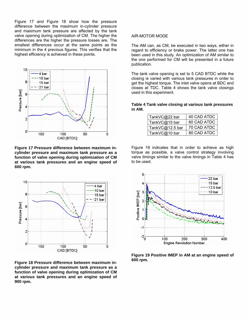
Figure 17 and Figure 18 show how the pressure difference between the maximum in-cylinder pressure and maximum tank pressure are affected by the tank valve opening during optimization of CM. The higher the differences are the higher the pressure losses are. The smallest differences occur at the same points as the minimum in the 4 previous figures. This verifies that the highest efficiency is achieved in these points.
Figure 17 Pressure difference between maximum in-cylinder pressure and maximum tank pressure as a function of valve opening during optimization of CM at various tank pressures and an engine speed of 600 rpm.
Figure 18 Pressure difference between maximum in-cylinder pressure and maximum tank pressure as a function of valve opening during optimization of CM at various tank pressures and an engine speed of 900 rpm.
AIR-MOTOR MODE
The AM can, as CM, be executed in two ways, either in regard to efficiency or brake power. The latter one has been used in this study. An optimization of AM similar to the one performed for CM will be presented in a future publication.
The tank valve opening is set to 5 CAD BTDC while the closing is varied with various tank pressures in order to get the highest torque. The inlet valve opens at BDC and closes at TDC. Table 4 shows the tank valve closings used in this experiment.
Table 4 Tank valve closing at various tank pressures in AM.
TankVC@22 bar 40 CAD ATDCTankVC@15 bar 60 CAD [email protected] bar 70 CAD ATDCTankVC@10 bar 80 CAD ATDC
Figure 19 indicates that in order to achieve as high torque as possible, a valve control strategy involving valve timings similar to the valve timings in Table 4 has to be used.
Figure 19 Positive IMEP in AM at an engine speed of 600 rpm.

Figure 20 Mean tank pressure during AM at an engine speed of 600 rpm.
It can be seen in Figure 20 that when the pressure is as high as 22 bars, it lasts for over 40 seconds at the current engine speed and valve timings. This time duration can be extended if the tank valve duration is decreased and thereby the AM efficiency would be increased.
Notice that when the tank pressure reaches a value below 4.5 bars, IMEP becomes negative. This is due to wrong tank or inlet valve timings. The amount of pressurized air charged into the cylinder is not enough in order to expand it to atmospheric pressure at BDC. Instead the pressure will decrease bellow atmospheric pressure and since the inlet valve opens at BDC there will be a blowdown of atmospheric air into the cylinder which leads to negative IMEP. This event is illustrated in Figure 21. In order to avoid this, the inlet valve should not open until the cylinder pressure reaches atmospheric pressure. Another way to avoid negative IMEP in this case is to have longer tank valve duration. In this way the cylinder pressure will reach atmospheric pressure at BDC and the inlet valve can then open at BDC without any backflow of atmospheric air into the cylinder.
Figure 21 PV-diagram illustrates why IMEP is below 0 bars at some point during AM.
REGENERATIVE EFFICIENCY
In order to estimate the potential of the pneumatic hybrid, the regenerative efficiency has to be calculated. The regenerative efficiency is defined as the ratio between the energy produced during AM and the energy stored during CM. It can also be defined as the ratio between the positive and negative IMEP:
−
+=IMEPIMEP
regenη (2)
It can also be interesting to see the efficiencies for every revolution during CM and AM. They are defined as:
−
=engine
CMtankCM P
P ,η (3)
and
AMtank
engineAM P
P
,
+=η (4)
where Pengine- is the engine motoring power during CM and Pengine+ is the engine brake power during AM.
Ptank in (3) and (4) is defined as the change of energy in the tank per time unit:
t
EPP stored
AMtankCMtank ΔΔ
=−= ,, (5)
Figure 22 and Figure 23 show the efficiency in CM and AM, respectively. The reason why all the efficiency curves are going towards zero in Figure 23 is that IMEP

is going towards 0 bars. These really low, near zero, efficiencies are not desirable and it is then better to use the remaining pressurized air to supercharge the engine as described by Schechter et al. [1, 4].
Figure 24 and Figure 25 show the total efficiency in CM and AM, respectively.
Figure 22 Compressor efficiency calculated for every engine revolution during CM at three different engine speeds.
Figure 23 Air-motor efficiency calculated for every engine revolution during CM at various tank pressures and at an engine speed of 600 rpm
Figure 24 Total compressor efficiency as a function of engine revolutions during CM at three different engine speeds.
Figure 25 Total air-motor efficiency as a function of engine revolutions during CM at various tank pressures and an engine speed of 600 rpm.
Next step is to calculate the regenerative efficiency. First thing to do is to calculate how much work has been used in order to compress air from 5 bars to 22 bars in the three different CM runs. These numbers have been chosen because the starting tank pressure in AM is about 22 bars and 5 bars corresponds to the remaining air pressure when IMEP is around zero in AM. The total work used during CM is then divided with the total work recovered during AM. The calculated regenerative efficiency can be seen in Table 5 and the results shows that the run at 900 rpm was the most optimized as stated in one of the previous sections.
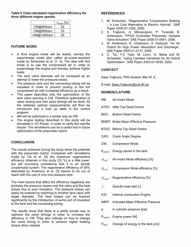
Table 5 Total calculated regenerative efficiency for three different engine speeds.
ηregen [%] CM@600rpm 32 CM@900rpm 33 CM@1200rpm 25
FUTURE WORK
• A third engine mode will be tested, namely the supercharge mode also called air-power-assisted mode by Schechter et al. [1, 4]. The idea with this mode is to use the compressed air in order to supercharge the engine and thereby achieve higher loads.
• The tank valve diameter will be increased as an attempt to lower the pressure losses.
• The pressure tank and the connecting tubing will be insulated in order to prevent cooling of the hot compressed air with increased efficiency as a result.
• This paper describes only the optimization of the tank valve opening in CM. Therefore optimization of valve closing and inlet valve timings will be done. All the obtained optimal measurements will then be introduced into a look up table in the control program.
• AM will be optimized in a similar way as CM. • The engine testing described in this study will be
simulated in GT-Power, in order to verify the real-life results. The simulations can be a useful tool in future optimization of the pneumatic hybrid.
CONCLUSION
The results achieved during the study show the potential with the pneumatic hybrid. Compared with simulations made by Tai et al. [4] the maximum regenerative efficiency obtained in this study (33 %) is a little lower, but still promising considering that it is an almost unoptimized system. The regenerative efficiency of 55% described by Anderson et al. [3] seems to be out of reach with the use of only one pressure tank.
The main factors that affect the efficiency negatively are probably the pressure losses over the valve and the heat losses due to poor insulation. The pressure losses can easily be lowered by switching to another tank valve with larger diameter. The heat losses can be lowered significantly by the introduction of some sort of insulation to the tank and the connecting tubing.
The results show that there is a pretty simple way to optimize the valve timings in order to increase the efficiency in CM. They also indicate on how to change the valve timing in order to achieve higher braking torque when needed.
REFERENCES
1. M. Schechter, “Regenerative Compression Braking – a Low Cost Alternative to Electric Hybrids”, SAE Paper 2000-01-1025, 2000.
2. S. Trajkovic, A. Milosavljevic, P. Tunestål, B. Johansson, “FPGA Controlled Pneumatic Variable Valve Actuation” SAE Paper 2006-01-0041, 2006.
3. M. Andersson, B. Johansson, A. Hultqvist, “An Air Hybrid for High Power Absorption and Discharge”, SAE Paper 2005-01-2137, 2005.
4. C. Tai, T-C Tsao, M. Levin, G. Barta and M. Schechter, “Using Camless Valvetrain for Air Hybrid Optimization”, SAE Paper 2003-01-0038, 2003.
CONTACT
Sasa Trajkovic, PhD student, Msc M. E.
E-mail: [email protected]
NOMENCLATURE
AM: Air-motor Mode
ATDC: After Top Dead Centre
BDC: Bottom Dead Centre
BMEP: Brake Mean Effective Pressure
BTDC: Before Top Dead Centre
CAD: Crank Angle Degree
CM: Compressor Mode
Estored: Energy stored in the tank
AMη : Air-motor Mode efficiency [%]
CMη : Compressor Mode efficiency [%]
regenη : Regenerative efficiency [%]
γ : Specific heat ratio [-]
ICE: Internal combustion Engine
IMEP: Indicated Mean Effective Pressure
p: In-cylinder pressure [bar]
Pengine: Engine power [W]
Ptank: Change of energy in the tank [J/s]

t: Time [s]
TDC: Top Dead Centre
RPM: Revolutions Per Minute
V: Cylinder volume [m3]

Paper 2

2008-01-1715
Investigation of Different Valve Geometries and Valve Timing Strategies and their Effect on Regenerative Efficiency for a
Pneumatic Hybrid with Variable Valve Actuation
Sasa Trajkovic, Per Tunestål and Bengt Johansson Division of Combustion Engines, Lund University, Faculty of Engineering
Copyright © 2008 SAE International
ABSTRACT
In the study presented in this paper a single-cylinder Scania D12 diesel engine has been converted to work as a pneumatic hybrid. During pneumatic hybrid operation the engine can be used as a 2-stroke compressor for generation of compressed air during vehicle deceleration and during vehicle acceleration the engine can be operated as an air-motor driven by the previously stored pressurized air.
The compressed air is stored in a pressure tank connected to one of the inlet ports. One of the engine inlet valves has been modified to work as a tank valve in order to control the pressurized air flow to and from the pressure tank.
In order to switch between different modes of engine operation there is a need for a VVT system and the engine used in this study is equipped with pneumatic valve actuators that uses compressed air in order to drive the valves and the motion of the valves are controlled by a combination of electronics and hydraulics.
This paper describes the introduction of new tank valve geometry to the system with the intent to increase the pneumatic hybrid regenerative efficiency. The new tank valve has a larger valve head diameter than the previously used setup described in [1], in order to decrease the pressure drop over the tank valve. In order to ensure tank valve operation during high in-cylinder pressures the valve is combined with an in-house developed pneumatic valve spring which makes the tank valve pressure compensated.
A comparison between the old and the new tank valve geometry and their effect on the pneumatic hybrid efficiency has been done. Also, optimization of the valve timings for both CM (Compressor Mode) and AM (Air-motor Mode) has been done in order to achieve further improvements on regenerative efficiency.
INTRODUCTION
As the pollution standards are becoming more stringent going towards zero emissions together with increasing fuel prices, engine developers are looking for alternative engine management to meet the increasing demand for better fuel economy. Of great importance is to improve the fuel economy at part-load, especially during city driving since it involves frequent acceleration and deceleration. In conventional vehicles all the kinetic energy built up during acceleration is lost during declaration in the form of heat generated by the friction brakes. This leads to a higher fuel consumption during city driving compared with freeway driving where acceleration and deceleration is less frequent.
Today there are several solutions to meet the demand for better fuel economy and one of them is electric hybrids. The idea with electric hybridization is to reduce the fuel consumption by taking advantage of the, otherwise lost, brake energy. Hybrid operation in combination with engine downsizing can also allow the combustion engine to operate at its best operating points in terms of load and speed.
An electric hybrid consists of two power sources, an ICE (Internal Combustion Engine) and an electric motor that can be used separately or combined. During deceleration the electric motor transforms the kinetic energy of the vehicle to electric power which it then stores in the batteries. The energy stored in the batteries will then be used when the vehicle accelerates. The main disadvantage with electric hybrids is that they require an extra propulsion system and large heavy battery. All this costs the manufacturers a lot of money, which is compensated by a higher end-product price.
One way of keeping the extra cost as low as possible compared to a conventional vehicle, is the introduction of pneumatic hybrid. It doesn’t require an expensive extra propulsion source and it works in a way similar to the electric hybrid. During deceleration of the vehicle, the

engine is used as a compressor that converts the kinetic energy contained in the vehicle into energy in the form of compressed air which is stored in a pressure tank. After a standstill the engine is used as an air-motor that utilizes the pressurized air from the tank in order to accelerate the vehicle. During a full stop the engine can be shut off.
Tai et al. [2] describes simulations with a so called “round-trip” efficiency of 36% and an improvement of 64% on fuel economy in city driving. Simulations made by Andersson et al. [3] show a regenerative efficiency as high as 55% for a dual pressure tank system for heavy vehicles. Real engine studies made by Trajkovic et al. [1] shows that the pneumatic hybrid has a promising potential in the reality and a regenerative efficiency of 33% has been achieved.
All these features of the pneumatic hybrid contribute to lower fuel consumption and in combination with the simplicity of the system, the pneumatic hybrid can be a promising alternative to the traditional vehicles of today and a serious contender to the better known electric hybrid.
PNEUMATIC HYBRID
Pneumatic hybrid operation introduces new operating modes in addition to conventional ICE operation. The main idea with pneumatic hybrid is to use the ICE in order to compress atmospheric air and store it in a pressure tank when retarding the vehicle. The stored compressed air can then be used either to accelerate the vehicle or to supercharge the engine in order to achieve higher loads when needed. The pneumatic hybrid also makes it possible to completely shut off the engine at idling like for instance at a stoplight, which in turn contributes to lower fuel consumption. [2,4,5,6]
In this study a single-cylinder engine was used. In reality, in for instance a heavy duty truck, one cylinder will not be enough to take full advantage of the pneumatic hybrid. A pneumatic hybrid will most probably utilize multiple cylinders. The number of cylinders that will be converted for pneumatic hybrid operation for a certain vehicle is hard to estimate at this point. It depends on, among other things, the vehicle weight and the maximum braking torque needed. Drive cycle simulations using data from engine experiments obtained in this study will be conducted in a near future in order to find optimal parameters like required number of converted cylinders and optimal tank volume, just to mention a few.
PNEUMATIC VARIABLE VALVE ACTUATION
In order to be able to switch between all pneumatic hybrid operations and conventional ICE operations, a variable valve actuating system is needed. In this study a pneumatic variable valve actuating system has been used. The valve system is designed and manufactured by a Swedish company named Cargine Engineering AB.
The system uses compressed air in order to drive the valves and the motion of the valves are controlled by a combination of electronics and hydraulics. The system is a fully variable valve actuating system, which means that the valve lift, valve timing and valve lift duration can be completely controlled, independently of each other. The pneumatic valve system in question and the control program has been more thoroughly described by Trajkovic et al. [7].
TANK VALVE
In order to run the engine as a pneumatic hybrid, a pressure tank has to be connected to the cylinder head. Tai et al. [2] describes an intake air switching system in which one inlet valve per cylinder is feed by either fresh intake air or compressed air from the pressure tank. Andersson et al. [3] describes a dual valve system where one of the intake ports has two valves, one of whom is connected to the air tank. A third solution would be to add an extra port to the cylinder head, which would be connected to the air tank. Since these three solutions demand significant modifications to a standard engine a simpler solution, where one of the existing inlet valves has been converted to a tank valve, has been chosen for this study. Since the engine used in this study has separated air inlet ports, there will be no interference between the intake system and the compressed air system. The drawback with this solution is that there will be a significant reduction in peak power, and reduced ability to generate and control swirl for good combustion.
MODES OF ENGINE OPERATION
The main pneumatic hybrid vehicle operations are compressor mode (CM) and air-motor mode (AM). Both modes have been tested in the study described in this paper and an attempt to optimize them has been carried out. The optimization of both CM and AM will be presented later on in this paper.
COMPRESSOR MODE
In CM the engine is used as a 2-stroke compressor in order to decelerate the vehicle. The kinetic energy of the moving vehicle is converted to potential energy in the form of compressed air.
During CM the inlet valve opens a number of CAD after TDC and brings fresh air to the cylinder, and closes around BDC. The moving piston starts to compress the air contained in the cylinder after BDC and the tank valve opens somewhere between BDC and TDC, depending on how much braking torque is needed, and closes shortly after TDC. The compressed air generated during CM is stored in a pressure tank that is connected to the cylinder head.
AIR-MOTOR MODE
In AM the engine is used as a 2-stroke air-motor that uses the compressed air from the pressure tank in order

to accelerate the vehicle. The potential energy in the form of compressed air is converted to mechanical energy on the crankshaft which in the end is converted to kinetic energy.
During AM the tank valve opens at TDC or shortly after and the compressed air fills the cylinder to give the torque needed in order to accelerate the vehicle. Somewhere between TDC and BDC the tank valve closes, depending on how much torque the driver demands. Increasing the tank valve duration will increase the torque generated by the compressed air. The inlet valve opens around BDC in order to avoid compression.
PRESSURE COMPENSATED TANK VALVE
In experiments done by Trajkovic et al. [1], one of the intake valves was chosen to work as tank valve. The intake valve had to be modified in order to make it possible to achieve desired TankVO (Tank Valve Opening) at high in-cylinder pressures. The tank valve diameter had to be reduced from the original size of 45 mm, down to 16 mm. Also the tank valve spring preloading had to be changed from 100 N to 340 N in order to keep the tank valve completely closed at tank pressures up to 25 bars. Both modifications lead to some complications. The reduced valve diameter increases the pressure losses over the tank valve and thus the regenerative efficiency will be reduced. The increased spring pre-loading will affect the pneumatic valve actuator energy consumption, but this is only of importance in a real vehicle where the actuators have to be feed with pressurized air from a compressor.
In an attempt to avoid the pressure losses over the tank valve, an in-house designed pneumatic valve spring has been developed and has replaced the conventional tank valve spring. Figure 1 shows a simple cross section illustration of the pneumatic valve spring arrangement mounted on the cylinder head. The pneumatic spring is constructed in such way, that it uses the tank pressure to keep the valve closed. A cylinder (indicated by number 1) is placed on the top of the cylinder head (indicated by number 4), with the tank valve (indicated by number 3) in the center of the cylinder. The cylinder is sealed in the bottom against the cylinder head and on the top the cylinder is sealed with the valve spring retainer (indicated by number 2). The space between the bottom sealing and the tank valve spring retainer is the pneumatic valve spring and it is connected to the tank valve port (indicated by number 6) and thus to the compressed air through 4 passages machined on the tank valve (indicated by number 5). The pressurized air enters the air passages on the valve and is guided up to the pneumatic valve spring, as indicated by the blue arrows. The passages are made in such way, that the pneumatic spring will be connected to the tank valve port at any time and any valve lift. Since the compressed air in the pneumatic spring works on the underside of the tank valve spring retainer and the compressed air in the tank valve port acts on the upside of the tank valve
head, as indicated by the yellow arrows, the net force should be zero, and thus the valve should be pressure compensated. This means that the tank will be kept closed without using any valve spring and the valve diameter can now be increased in order to reduce the pressure drop over the valve. In the study presented in this paper, the tank valve diameter has been increased to 28 mm, which is almost the double of what has been used before. Figure 2 shows a picture of the two tank valves used in this study. Geometrical properties of the pneumatic spring arrangement can be seen in Table 1.
Figure 1 A simple cross section illustration of the pneumatic valve spring arrangement mounted on the cylinder head When the valve is open the force generated by the pressurized air acting on the upside of the tank valve head is canceled. This means that there now only exist a considerable force on the undersurface of the valve spring retainer trying to close the tank valve. In order to overcome this problem, the tank valve actuator is feed with compressed air from the tank. This means that the pressure at a certain time is the same in the pneumatic valve spring as in the valve actuator. Since the actuator piston has a larger diameter than the tank valve spring retainer, the actuator will always have enough power to open the valve and maintain it open for as long as desired.
1
3
2
4
5
6
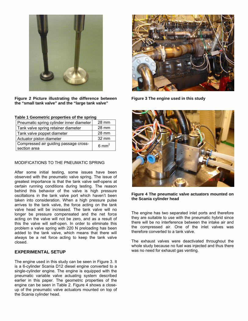
Figure 2 Picture illustrating the difference between the “small tank valve” and the “large tank valve”
Table 1 Geometric properties of the spring Pneumatic spring cylinder inner diameter 28 mm Tank valve spring retainer diameter 28 mm Tank valve poppet diameter 28 mm Actuator piston diameter 32 mm Compressed air guiding passage cross-section area 6 mm2
MODIFICATIONS TO THE PNEUMATIC SPRING
After some initial testing, some issues have been observed with the pneumatic valve spring. The issue of greatest importance is that the tank valve self-opens at certain running conditions during testing. The reason behind this behavior of the valve is high pressure oscillations in the tank valve port which haven’t been taken into consideration. When a high pressure pulse arrives to the tank valve, the force acting on the tank valve head will be increased. The tank valve will no longer be pressure compensated and the net force acting on the valve will not be zero, and as a result of this the valve will self-open. In order to eliminate this problem a valve spring with 220 N preloading has been added to the tank valve, which means that there will always be a net force acting to keep the tank valve closed.
EXPERIMENTAL SETUP
The engine used in this study can be seen in Figure 3. It is a 6-cylinder Scania D12 diesel engine converted to a single-cylinder engine. The engine is equipped with the pneumatic variable valve actuating system described earlier in this paper. The geometric properties of the engine can be seen in Table 2. Figure 4 shows a close-up of the pneumatic valve actuators mounted on top of the Scania cylinder head.
Figure 3 The engine used in this study
Figure 4 The pneumatic valve actuators mounted on the Scania cylinder head
The engine has two separated inlet ports and therefore they are suitable to use with the pneumatic hybrid since there will be no interference between the intake air and the compressed air. One of the inlet valves was therefore converted to a tank valve.
The exhaust valves were deactivated throughout the whole study because no fuel was injected and thus there was no need for exhaust gas venting.

Table 2 Engine geometric properties
Displaced Volume 1966 cm3 Bore 127.5 mm Stroke 154 mm Connecting Rod Length 255 mm Number of Valves 4 Compression Ratio 18:1 Piston type Flat Inlet valve diameter 45 mm Tank valve diameter 16 and 28 mm Piston clearance 7.3 mm
The pressure tank used in this study is an AGA 50 litre pressure tank suitable for pressures up to 200 bars and it is shown in Figure 5. The pressure tank is connected to the cylinder head by metal tubing. In order to eliminate the metal tubing as a potential bottleneck on account of air flow choking, the diameter of the tubing was doubled at the same time as the small tank valve was replaced by the large tank valve. The tank size in the current system is selected based on availability rather than optimality, but in the future the tank volume will be an important parameter for the optimization of the system.
Figure 5 The pressure tank connected to the cylinder head by metal tubing
Table 3 shows some valve parameters. The maximum valve lift height in this study is limited to 7 mm in order to avoid valve to piston contact. The valve system can, when unlimited, offer a valve lift height of about 12 mm.
Table 3 Valve parameters
Inlet valve supply pressure 4 bar Tank valve supply pressure 6 bar Hydraulic brake pressure 4 bar Inlet valve spring preloading 100 N Tank valve spring preloading 220 N Maximum valve lift 7 mm
Since the pneumatic valve spring arrangement require the actuator to be fed by compressed air from the tank, an extra pressurized air supply line had to be added. A problem with the actuator being fed with tank pressure is that there is a pressure threshold below which the pneumatic valve actuator will not work as expected. This means that the actuator has to be fed with compressed air from an external source. This adds thereby the need of having a pressure source switch. The switching system used in this study is built up by two check-valves which are arranged in such way that the source feeding the valve actuator will always be the source with the highest pressure. For instance if the external source of compressed air is set to 6 bars it will be the main feeding source until the pressure in the pressure tank exceeds 6 bars. A picture of the pressure source switching system is shown in Figure 6.
Figure 6 Pressurized air switching system built up by two check-valves
ENGINE EXPERIMENTAL RESULTS
Both CM and AM have been tested in the study described in this paper. Main focus have been on the optimization of CM and AM and comparison between the old and new setup. The results will be discussed thoroughly. Note that all presented pressure values are absolute and IMEP is given in 2-stroke scale.
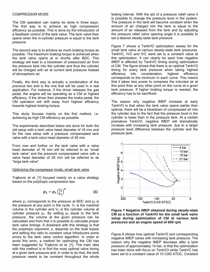
COMPRESSOR MODE
The CM operation can mainly be done in three ways. The first way is to achieve as high compression efficiency as possible. This is done by the introduction of a feedback control of the tank valve. The tank valve then opens when the in-cylinder pressure is equal to the tank pressure.
The second way is to achieve as much braking torque as possible. The maximum braking torque is achieved when the tank valve opens at or shortly after BDC. This strategy will lead to a blowdown of pressurized air from the pressure tank into the cylinder and thus the cylinder will be charged with air at current tank pressure instead of atmospheric air.
Finally, the third way is actually a combination of the previous two and is the one that will be used in a real application. For instance, if the driver releases the gas pedal, the engine will be operating as a CM at highest efficiency. If the driver then presses the brake pedal, the CM operation will drift away from highest efficiency towards highest braking torque.
This study focuses mainly on the first method, i.e. achieving as high CM efficiency as possible.
The experiments described below are done for both the old setup with a tank valve head diameter of 16 mm and for the new setup with a pressure compensated tank valve with a tank valve head diameter of 28 mm.
From now and further on the tank valve with a valve head diameter of 16 mm will be referred to as “small tank valve” and the pressure compensated valve with a valve head diameter of 28 mm will be referred to as “large tank valve”.
Optimizing the compressor mode, small tank valve
Trajkovic et al. [1] focused mainly on a valve strategy based on the polytro ic ssion law: p compre
(1)
where p1 corresponds to the pressure at BDC and p2 is the pressure at any point in the cycle. V1 is the maximal volume in the cylinder and V2 is the cylinder volume at cylinder pressure p2. By setting p2 equal to the tank pressure, the volume at the given pressure can be calculated and from that it is possible to calculate proper tank valve timings. A drawback with this strategy is that the polytropic exponent, κ, depends on the heat losses and setting this ratio to constant value introducers some errors to the tank valve control algorithm. In order to avoid this error, a method for optimizing the CM has been suggested by Trajkovic et al. [1]. The main idea with this method is to find the most optimal valve timing at a given tank pressure and, in order to do that, the tank pressure needs to be constant throughout the whole
testing interval. With the aid of a pressure relief valve it is possible to change the pressure level in the system. The pressure in the tank will become constant when the amount of air charged into the tank is equal to the amount of air released from the tank and by adjusting the pressure relief valve opening angle it is possible to set a desired steady-state tank pressure.
Figure 7 shows a TankVO optimization sweep for the small tank valve at various steady-state tank pressures. TankVC, IVO and IVC were set to a constant value at this optimization. It can clearly be seen how negative IMEP is affected by TankVO timing during optimization of CM. The figure shows that there is an optimal TankVO timing for every tank pressure when taking highest efficiency into consideration, highest efficiency corresponds to the minimum in each curve. This means that it takes less power to compress the inducted air at this point than at any other point on the curve at a given tank pressure. If higher braking torque is needed, the efficiency has to be sacrificed.
The reason why negative IMEP increase at early TankVO is that when the tank valve opens earlier than optimal, there will be a blowdown of compressed air into the cylinder due to the fact that the pressure level in the cylinder is lower than in the pressure tank. At a certain premature TankVO, negative IMEP will dramatically increase with increasing tank pressure, due to a larger pressure level difference between the cylinder and the pressure tank.
Figure 7 Negative IMEP obtained during steady-state CM as a function of TankVO for the small tank valve setup during optimization of CM at various tank pressures and an engine speed of 600 rpm
Figure 8 shows how optimal TankVO and corresponding negative IMEP varies with increasing tank pressure. The reason why the negative IMEP decrease after a tank pressure of approximately 14 bar, is that the optimization has been done with focus on TankVO while TankVC has been set to a constant value of 10 CAD ATDC. Constant

TankVC will affect the negative IMEP at higher tank pressures because ideally TankVC should be retarded towards TDC with increasing tank pressure. IVO should be set in such way that the pressurized air trapped in the cylinder after TankVC will be expanded to atmospheric pressure. At higher tank pressures, a late TankVC means that the in-cylinder pressure is higher than desired, and this excess pressure pushes the piston as it moves towards BDC and thereby contributes with positive IMEP which decreases the negative IMEP for the whole cycle.
Figure 8 TankVO and negative IMEP as a function of tank pressure for the small tank valve setup at an engine speed of 600 rpm
Figure 9 Comparison of negative IMEP for unoptimized and optimized TankVO as a function of engine cycle number during CM operation for the small tank valve setup. End tank pressure is about 21 bars in both cases
CM operation testing has been done both with an unoptimized tank valve, i.e. the feedback control of the tank valve was based on equation (1), and with the optimal TankVO timings seen in Figure 8. The result can
be seen in Figure 9 where negative IMEP for both the unoptimized tank valve and the optimized tank valve is shown. Initially, negative IMEP for the unoptimized tank valve is similar to negative IMEP for the optimized tank valve, but after about 300 engine cycles negative IMEP for the optimized tank valve remains reasonably constant while negative IMEP for the unoptimized tank valve continues to increase throughout the rest of the test.
The reason why negative IMEP is decreasing during optimized tank valve operation between 600 and 800 engine cycles is that the optimization is based on the valve timings shown in Figure 8, and thus the same IMEP behavior is expected.
Optimizing the compressor mode, large tank valve
In order to reduce the pressure drop over the tank valve the small valve has been replaced with a valve that has a larger valve head diameter in combination with the previously described pneumatic spring arrangement.
Figure 10 Negative IMEP obtained during steady-state CM as a function of TankVO for the large tank valve setup at various tank pressures for engine speeds of 600 and 900 rpm
Figure 10 shows a TankVO optimization sweep for the large tank valve at various steady-state tank pressures, similar to the TankVO sweep in Figure 7. With the larger valve, the negative IMEP at a tank pressure of 4 bar and at optimal TankVO for both 600 and 900 rpm is lower compared to the negative IMEP in Figure 7 at the same tank pressure. This is because the pressure drop is decreased due to the larger tank valve head diameter. At 10 and 15 bars, there is hardly any difference between negative IMEP for the large tank valve compared to the small tank valve. The only difference is that the optimal TankVO for the large tank valve is advanced a number of CAD compared to TankVO for the small valve. One of the reasons for this behavior is most likely that there is a blowdown of pressurized air into the cylinder through the

tank valve. It seems as the tank valve is not completely pressure compensated as expected and thus there exist a net force acting to open the tank valve. Another reason is that there is some pressure losses in the pressurized air supply line between the tank and the pneumatic valve actuator, which means that the pressurized air fed to the valve actuator at a certain time is not the same as the mean tank pressure at the corresponding time and therefore the ability to open the tank valve at optimal timing is lost and has to be advanced. An advance in TankVO compared to optimal timing means that there will be a blowdown of pressurized air into the cylinder and thus negative IMEP will increase. The reason why negative IMEP for the large tank valve is considerably lower than for the small tank valve at 4 bars tank pressure is that at this tank pressure level, the actuator is fed with 6 bars of compressed air from an external source. This means that, at this point there is a surplus of 2 bars feeding the valve actuator and thus the optimal TankVO timing can be achieved.
Another observation that can be made from Figure 10 is that at a certain tank pressure, there is a difference in negative IMEP between the case at 600 rpm and the case at 900 rpm. The reason is that at a higher engine speed, there will be less time for the blowdown process previously described and thereby its effect on the negative IMEP will be less.
Figure 11, Figure 12 and Figure 13 show how optimal TankVO and corresponding negative IMEP varies with increasing tank pressure at various engine speeds for the large tank valve setup. Comparing negative IMEP from Figure 11 with negative IMEP from Figure 8 indicates that the pressure losses over the valve are lower with the large valve than with the small valve. If focus is put on the TankVO, it can clearly be seen that the optimal TankVO for the large tank valve is occurs considerably earlier compared to the optimal TankVO for the small tank valve. The reason for this behavior can once again be explained as inadequate amount of pressurized air supplied to the tank valve actuator and therefore the valve timing has to be advanced a number of CAD away from the real optimum, which contributes to a higher negative IMEP.
It can also be seen that TankVO advances with engine speed at the same tank pressure with the reason being the same as stated previously. As the engine speed increase, the pressure tank charging rate increase faster than the supply rate of compressed air to the actuator due to restrictions in the pressurized air supply line between the pressure tank and the valve actuator. The result is that at a certain time, mean tank pressure will be higher than actuator supply pressure. As engine speed increase, the pressure difference between the tank pressure and the actuator supply pressure will also increase. Therefore TankVO has to be advanced with increasing engine speed.
Figure 11 Optimized TankVO timing and corresponding negative IMEP during CM optimization as a function of tank pressure for the large tank valve setup at an engine speed of 600 rpm
Figure 12 Optimized TankVO timing and corresponding negative IMEP during CM optimization as a function of tank pressure for the large tank valve setup at an engine speed of 900 rpm
Notice that at a tank pressure of 4 bars, negative IMEP at all three engine speeds presented in Figure 11, Figure 12 and Figure 13, are lower than negative IMEP shown in Figure 8. This is once again due to the surplus of 2 bars in the pressurized air supply line feeding the tank valve actuator since the compressed air source is external with an air pressure set to 6 bars. This indicates that in order to achieve optimal TankVO timing, there should always be a surplus of minimum 2 bars in the supply line to compensate for all the pressure losses through it.

Figure 13 Optimized TankVO timing and corresponding negative IMEP during CM optimization as a function of tank pressure for the large tank valve setup at an engine speed of 1200 rpm
Comparing Figure 11, Figure 12 and Figure 13 with one another indicates that at equal tank pressure, negative IMEP increases with engine speed. This is due to the fact that with increasing engine speed there is less time to vent the cylinder from compressed air and thus there will be an overshoot in cylinder pressure which increases with increasing engine speed. This is illustrated in Figure 14.
Figure 14 PV-diagram during CM for three different engine speeds at 4 bars of tank pressure
Figure 15 shows negative IMEP during optimal CM at three different engine speeds for the large tank valve setup. Comparing the result displayed in Figure 15 with the result from the optimized test shown in Figure 9 indicates that there is only a difference the first 200 cycles. The results obtained with the large tank valve shows that IMEP is lower than the corresponding results
obtained with the small tank valve which verifies that increasing the tank valve diameter decreases the pressure drop over the tank valve. The reason why negative IMEP is almost the same in both cases after 200 cycles is probably once again insufficient pressure in the compressed air supply line feeding the tank valve actuator.
Figure 15 Negative IMEP during optimal CM as a function of engine cycle number at three different engine speeds for the tank valve setup
The corresponding mean tank pressure as a function of engine cycle number at three different engine speeds can be seen in Figure 16. There is a slight difference between the curves. The end pressure at 900 rpm is higher than at both 600 and 1200 rpm. This can probably be explained with tank pressure leakage into the cylinder through the tank valve. This would mean that there exists a net force acting to open the tank valve and in that case the tank valve is not pressure compensated. Since leakage of compressed air through an orifice is constant in time at a constant pressure, the amount of air inducted into the cylinder per cycle due to leakage will decrease with increasing engine speed, and thus the end tank pressure should reach a higher level. At 1200 rpm, this explanation is not enough since the end tank pressure is at the same level as at 600 rpm. Careful observation of the tank pressure curve at 1200 rpm in Figure 16, indicates that it follow the tank pressure curve at 900 rpm quite well up to approximately 600 engine cycles and then it starts to deviate and ends at the same pressure level as at 600 rpm. The reason is probably that, during this specific test run, the tank valve actuator didn’t behave as expected. This can be verified from Figure 15, where negative IMEP at 1200 rpm starts to decrease at about 600 cycles. The reason for this behavior is that, due to inexplicable performance of the tank valve actuator, the duration of maximum valve lift abruptly decreases after 600 cycles, as displayed in Figure 17. A shorter duration means that there will not be enough time to vent the cylinder on pressurized air and therefore the cylinder will still be filled with pressurized air at tank valve closing. This excess of

compressed air pushes the piston as it moves towards BDC and thus contributes with positive IMEP, which in turn decreases negative IMEP for the whole cycle.
Figure 16 Mean tank pressure as a function of engine cycle number at three different engine speeds
Figure 17 Tank valve lift at two different engine cycles at an engine speed of 1200 rpm
Figure 18 and Figure 19 displays the port temperature immediately after the tank valve and the temperature in the pressure tank, respectively, at three different engine speeds. The results indicate that there is a considerable amount of heat losses through the system. The explanation is that the metal tubing, which connects the cylinder head with the tank, and the pressure tank are not heat insulated in any way. Therefore, a considerable amount of the total thermal energy generated during CM will be transferred to the surroundings and thus the total efficiency of the pneumatic hybrid will be decreased.
Figure 18 Temperature after tank valve (port temperature) as a function of engine cycle number at three different engine speeds
Figure 19 Pressure tank temperature as a function of engine cycle number at three different engine speeds Figure 20 and Figure 21 illustrates the pressure drop over the small tank valve and the large valve, respectively, obtained at three different engine speeds during CM. The hump-like behavior between 100 and 200 engine cycles at both 900 and 120 rpm in Figure 21 occurs due to the pressurized air source switching system described earlier. As the tank pressure is reaching a pressure level close to the switching pressure level, the tank valve lift height is decreasing, as can be seen in Figure 22. The tank valve lift has decreased by almost 1 mm at engine cycle 150 compared to cycle 100. At cycle 200 the tank valve lift height has nearly returned to a maximum. The reason for this behavior is thought to be bad interaction between the check-valves due to pressure oscillations in the pressurized air supply line. During normal running conditions one of the check-valves will be completely open, but during the transition period, both check-valves will open and close frequently

due to the pressure oscillations, which lead to a deficit in pressure and thus the valve lift will decrease.
Figure 20 Pressure difference between maximum in-cylinder pressure and maximum pressure after the tank valve (port pressure) as a function of engine cycle number at various speeds. Tank valve with small diameter was used during this test.
Figure 21 Pressure difference between maximum in-cylinder and maximum pressure after the tank valve (port pressure) as a function of engine cycle number at various engine speeds. Tank valve with large diameter was used during this test.
Another observation made from Figure 20 and Figure 21 is that the curves displayed in Figure 21 are indicating an increasing trend, while the curves in Figure 20 are decreasing or somewhat constant throughout the whole test. The reason is, as stated before, insufficient pressure in the pressurized air supply line feeding the tank valve actuator which forces TankVO to deviate from the optimal timing, and thereby the pressure difference between the pressure after the valve and the cylinder pressure will increase.
Figure 22 Tank valve lift at three different engine cycles and at an engine speed of 1200 rpm
Figure 23 and Figure 24 show cylinder pressure at a mean tank pressure of 8 bars for the small tank valve setup and the large tank valve setup, respectively. It can clearly be seen that the pressure losses over the small tank valve are considerably higher than they are with the larger tank valve. This is mainly because choking occurs over the small tank valve which limits the air flow and thereby the pressure will increase. Figure 23 and Figure 24 indicates that this overshoot in pressure can be lowered dramatically if the small tank valve diameter is increased.
Figure 23 In-cylinder pressure and tank pressure during CM with a small valve diameter at revolution 200 and an engine speed of 600 rpm
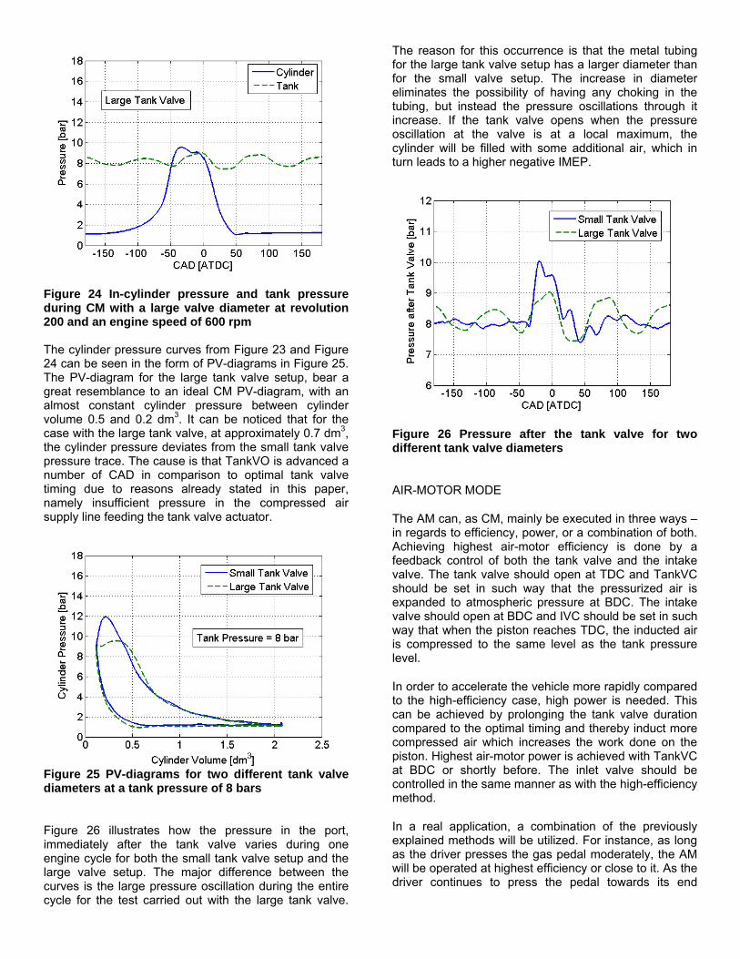
Figure 24 In-cylinder pressure and tank pressure during CM with a large valve diameter at revolution 200 and an engine speed of 600 rpm The cylinder pressure curves from Figure 23 and Figure 24 can be seen in the form of PV-diagrams in Figure 25. The PV-diagram for the large tank valve setup, bear a great resemblance to an ideal CM PV-diagram, with an almost constant cylinder pressure between cylinder volume 0.5 and 0.2 dm3. It can be noticed that for the case with the large tank valve, at approximately 0.7 dm3, the cylinder pressure deviates from the small tank valve pressure trace. The cause is that TankVO is advanced a number of CAD in comparison to optimal tank valve timing due to reasons already stated in this paper, namely insufficient pressure in the compressed air supply line feeding the tank valve actuator.
Figure 25 PV-diagrams for two different tank valve diameters at a tank pressure of 8 bars
Figure 26 illustrates how the pressure in the port, immediately after the tank valve varies during one engine cycle for both the small tank valve setup and the large valve setup. The major difference between the curves is the large pressure oscillation during the entire cycle for the test carried out with the large tank valve.
The reason for this occurrence is that the metal tubing for the large tank valve setup has a larger diameter than for the small valve setup. The increase in diameter eliminates the possibility of having any choking in the tubing, but instead the pressure oscillations through it increase. If the tank valve opens when the pressure oscillation at the valve is at a local maximum, the cylinder will be filled with some additional air, which in turn leads to a higher negative IMEP.
Figure 26 Pressure after the tank valve for two different tank valve diameters
AIR-MOTOR MODE
The AM can, as CM, mainly be executed in three ways – in regards to efficiency, power, or a combination of both. Achieving highest air-motor efficiency is done by a feedback control of both the tank valve and the intake valve. The tank valve should open at TDC and TankVC should be set in such way that the pressurized air is expanded to atmospheric pressure at BDC. The intake valve should open at BDC and IVC should be set in such way that when the piston reaches TDC, the inducted air is compressed to the same level as the tank pressure level.
In order to accelerate the vehicle more rapidly compared to the high-efficiency case, high power is needed. This can be achieved by prolonging the tank valve duration compared to the optimal timing and thereby induct more compressed air which increases the work done on the piston. Highest air-motor power is achieved with TankVC at BDC or shortly before. The inlet valve should be controlled in the same manner as with the high-efficiency method.
In a real application, a combination of the previously explained methods will be utilized. For instance, as long as the driver presses the gas pedal moderately, the AM will be operated at highest efficiency or close to it. As the driver continues to press the pedal towards its end

position, the AM operation will drift away from highest efficiency towards maximum air-motor power.
This study focuses mainly on the first method, namely achieving as high AM efficiency as possible.
Optimizing the air-motor mode
An attempt to use the polytropic compression law, in order to achieve a proper valve strategy during AM, has been done. TankVC is controlled in such way that at a certain tank pressure, a proper closing angle is calculated with the help of the polytropic relation. Also the IVC is calculated in a similar way. TankVO and IVO are set to a constant value of 0 CAD ATDC and 180 CAD BTDC, respectively. TankVC and corresponding positive IMEP obtained with this method can be seen in Figure 27. These results are quite poor compared to the results shown by Trajkovic et al [1], where IMEP levels of 4 bars have been shown with constant valve timings. The reason is that, as stated before, the specific-heat ratio depends on the heat losses and setting this ratio to a constant value introduces some errors to the valve control algorithm. Also, the polytropic relation doesn’t take the pressure losses over the tank valve into account, and therefore the TankVC will be chosen closer to TDC than what would be optimal.
Figure 27 TankVO and corresponding positive IMEP during AM as a function of tank pressure for the large tank valve setup at an engine speed of 600 rpm. TankVO timings are based on the polytropic relation. In order to optimize the AM, there is a need for a method that can help finding the optimal valve timings. The steady-state method, used for optimizing the CM, cannot be used in order to optimize the AM, since there is no charging of the pressure tank during AM and thereby a steady-state tank pressure cannot be achieved.
A method for finding the optimal IVC has been developed. The idea is to vary IVC and thus the corresponding peak cylinder pressure will also be varied.
In that way a map, containing IVC as a function of peak cylinder pressure can be created.
In order to find the optimal TankVC, results from the CM optimization, shown in Figure 11, have been used. During the compression stroke in CM, the atmospheric air in the cylinder is compressed to the same pressure level as the tank pressure level before the tank valve opens. In AM, the procedure should be the opposite. The pressure level in the cylinder is the same as the tank pressure level when the tank valve is supposed to close. The pressurized air is then expanded to the atmospheric pressure level. Thereby the results obtained during CM optimization can, with some modification, be used to control the valve during AM. In order to fit the results from CM to AM, some tuning of the valve timings had to be done.
Figure 28 shows the final results from AM testing where both IVC and TankVC have been optimized with the methods described above. Comparing the results from Figure 28 with the results from Figure 11 indicates that the curves bear a resemblance to one another. But there are some differences, mainly for the TankVC. For instance, at a tank pressure of 20 bars, the results in Figure 28 indicates a TankVC at approximately 33 CAD ATDC, while the results in Figure 11 indicates a TankVO at approximately 38 CAD BTDC. The difference of 6 CAD is due to the fact that IVC during AM is chosen in such way that the peak in-cylinder pressure is lower than the tank pressure when the tank valve opens, which can be seen in Figure 29. Thereby, the deficit in the pressurized air supply line is compensated for.
Figure 28 Optimized TankVO and corresponding positive IMEP during AM as a function of tank pressure for the large tank valve setup at an engine speed of 600 rpm

Figure 29 Illustration on the difference between the tank valve port pressure and the cylinder pressure at TankVO during AM operation Figure 30 shows positive IMEP obtained with two different tank valve setups and valve strategies during AM operation. The small tank valve curve has been obtained with the constant valve timings displayed in Table 4. The large tank valve curve has been obtained with the optimal valve timings shown in Figure 28. The starting tank pressure is about 20 bars in both cases. It can be realized that, an increase in valve head diameter together with optimal valve timings, has a large impact on the AM operation. This will in turn lead to a considerable increase in the AM total efficiency. The reason why IMEP for the large tank valve setup is much higher throughout the whole test compared to the small tank valve setup, is that the pressurized air is used in a much more efficient way. A larger tank valve diameter contributes to less pressure losses over the tank valve and an optimized valve control strategy contributes to a more efficient use of the pressurized air, and together they contribute to a higher positive IMEP.
Figure 30 Positive IMEP for two different tank valve setups and valve strategies as a function of engine cycle number at an engine speed of 600 rpm during AM operation
Table 4 Valve timing used for the small tank valve setup during AM operation
IVO [CAD BTDC] 180 IVC [CAD BTDC] 0 TankVO [CAD ATDC] -5 TankVC [CAD ATDC] 40
Figure 31 shows the tank pressure decrease for the small tank valve setup and large tank valve setup, obtained during the test displayed in Figure 30. With the large tank valve, the tank pressure decreases almost linearly. With the smaller valve, the tank pressure has a higher rate of discharge in the beginning, but after about 150 cycles the discharge rate starts to decrease. The reason for this behavior is that the valve timings with the small tank valve are set to a constant value. This means that in the beginning the tank valve duration is much longer than the optimal tank valve duration, and thereby the cylinder will be filled with more compressed air, thus leading to a higher rate of discharge of the tank pressure for this case. After a while, as the tank pressure decrease, the duration becomes too short and the cylinder is filled with less air than is optimal and thereby the tank pressure discharge will decrease.
Figure 31 Mean tank pressure for two different valve geometries at an engine speed of 600 rpm
Figure 32 and Figure 33 illustrates PV-diagrams for both tank valve setups at tank pressures 16.5 bars and 6.5 respectively. There are evident differences in peak cylinder pressure between the small tank valve setup and the large tank valve setup in both figures. The reason is that the flow over the small tank valve will become chocked due to a very restricted flow area. With the larger tank valve, the flow area is increased more than three times compared to the small tank valve flow area and therefore the threshold for choked flow has been raised. Another issue with constant tank valve timing, which can be seen in Figure 33, is that one portion of the PV-curve indicates negative IMEP. Too
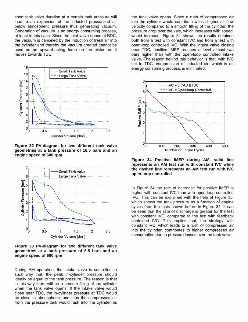
short tank valve duration at a certain tank pressure will lead to an expansion of the inducted pressurized air below atmospheric pressure thus generating vacuum. Generation of vacuum is an energy consuming process, at least in this case. Since the inlet valve opens at BDC, the vacuum is canceled by the induction of fresh air into the cylinder and thereby the vacuum created cannot be used as an upward-acting force on the piston as it moves towards TDC.
Figure 32 PV-diagram for two different tank valve geometries at a tank pressure of 16.5 bars and an engine speed of 600 rpm
Figure 33 PV-diagram for two different tank valve geometries at a tank pressure of 6.5 bars and an engine speed of 600 rpm
During AM operation, the intake valve is controlled in such way that, the peak in-cylinder pressure should ideally be equal to the tank pressure. The reason is that in this way there will be a smooth filling of the cylinder when the tank valve opens. If the intake valve would close near TDC, the in-cylinder pressure at TDC would be close to atmospheric, and thus the compressed air from the pressure tank would rush into the cylinder as
the tank valve opens. Since a rush of compressed air into the cylinder would contribute with a higher air flow velocity compared to a smooth filling of the cylinder, the pressure drop over the vale, which increases with speed, would increase. Figure 34 shows the results obtained both from a test with constant IVC and from a test with open-loop controlled IVC. With the intake valve closing near TDC, positive IMEP reaches a level almost two bars higher than with the open-loop controlled intake valve. The reason behind this behavior is that, with IVC set to TDC, compression of inducted air, which is an energy consuming process, is eliminated.
Figure 34 Positive IMEP during AM, solid line represents an AM test run with constant IVC while the dashed line represents an AM test run with IVC open-loop controlled
In Figure 34 the rate of decrease for positive IMEP is higher with constant IVC than with open-loop controlled IVC. This can be explained with the help of Figure 35, which shows the tank pressure as a function of engine cycles from the tests shown before in Figure 34. It can be seen that the rate of discharge is greater for the test with constant IVC, compared to the test with feedback controlled IVC. This implies that, the strategy with constant IVC, which leads to a rush of compressed air into the cylinder, contributes to higher compressed air consumption due to pressure losses over the tank valve.

Figure 35 Tank pressure during AM, solid line represents an AM test run with constant IVC while the dashed line represents an AM test run with IVC open-loop controlled
Figure 36 shows torque for both constant IVC and open-loop controlled IVC. The result is quite impressive for a 2-litre engine operating without any combustion. The reason behind the large difference in maximum torque between the curves is that due to that rushing compressed air flow hits the piston with a huge force when the tank valve opens. With feedback controlled IVC, compressed air enters the cylinder smoothly and therefore no shock force will be generated.
Figure 36 Torque during AM for both constant IVC timing and open-loop controlled IVC at an engine speed of 600 rpm Figure 37, Figure 38 and Figure 39 illustrates PV-diagrams for both intake valve strategies at tank pressures 16.5 bars and 6.5 respectively. The pressure curve, obtained with constant IVC, has an overshoot at TDC compared to the curve obtained with open-loop controlled IVC. The reason is that as the compressed air starts to rush into the cylinder, a pressure wave is
generated which propagates though the cylinder and out again through the open tank valve. A close-up of the PV-diagrams in Figure 37 is illustrated in Figure 38. It can clearly be seen that with constant IVC, the cylinder pressure overshoots at first and then decreases bellow the cylinder pressure obtained with open-loop controlled IVC. This indicates that there is a pressure wave propagating through the cylinder.
Figure 37 PV-diagram obtained during AM at a tank pressure of 16.5 bar and at an engine speed of 600 rpm, solid line represents an AM test run with constant IVC while the dashed line represents an AM test run with IVC open-loop controlled
Figure 38 Close-up of the PV-diagrams at a tank pressure of 16.5 bars shown in Figure 37

Figure 39 PV-diagram obtained during AM at a tank pressure of 6.5 bar and at an engine speed of 600 rpm, solid line represents an AM test run with constant IVC while the dashed line represents an AM test run with IVC open-loop controlled
REGENERATIVE EFFICIENCY
In order to estimate the potential of the pneumatic hybrid, and the possibility to compare different tests with each other, a regenerative efficiency has to be calculated. The regenerative efficiency is the ratio between the energy recovered during AM and the energy consumed during CM. It can also be defined as the ratio between p sitive d ative IMEP: o an neg
(2)
Table 5 show the regenerative efficiency with different tank valve setups and valve strategies at three engine speeds. The regenerative efficiency obtained with the small tank valve setup is retrieved from [1]. It has a maximum value of 33% at 900 rpm. The reason why the efficiency is higher at 900 rpm than at 600 rpm, as explained by Trajkovic et al. [1], is that the unoptimized feedback controller by coincidence is better suited for the case at 900 rpm than at 600 rpm. The regenerative efficiency for the large tank valve setup indicates that with optimized tank valve timing, the maximum efficiency occurs at 600 rpm and decreases with increasing engine speed. A tremendous improvement has been achieved while switching from the small tank valve setup to the large tank valve setup. The improvement mainly depends on a larger tank valve head diameter and optimized tank valve timing during AM. A change in inlet valve strategy from constant IVC to open-loop controlled IVC, increases the regenerative efficiency further.
The pneumatic tank valve actuator consumes energy in the form of compressed air from the pressure tank. Since its energy consumption decreases the total energy stored in the pressure tank, it has to be seen as energy losses. These losses have automatically been taken into
account in the calculation of regenerative efficiency. This is only valid for the large valve setup, since the pneumatic tank valve used in the small tank valve setup has been feed with compressed air generated from an external source. This means that the regenerative efficiency calculated for the large tank valve setup, is lower than it would be if the pneumatic valve actuator energy losses were excluded from the calculation.
Table 5 Calculated total regenerative efficiency for different tank valve setups and valve strategies at three different engine speeds ηregen
Engine speed 600 900 1200
Small tank valve setup 32 33 25
Large Tank valve setup, constant IVC during AM 44 40 37 Large tank valve setup 48 44 40
It should be noticed that the regenerative efficiency, described in this paper is actually an indicated efficiency, apart from the included pneumatic valve actuator energy losses. This means that a real vehicle cannot utilize the energy in the same extent due, among other things, to engine and driveline friction losses, which will lead to a lower regenerative efficiency.
CONCLUSION
A pressure compensated tank valve with a valve head diameter of 28 mm has been tested and evaluated. The pressure compensation has been achieved with an in-house developed pneumatic valve spring arrangement mounted on the cylinder head. The evaluation has shown that there exists some trouble with the pneumatic valve spring concerning tank valve actuation, mostly because the pneumatic valve actuator is driven by compressed air from the pressurize air. This can be resolved by the use of externally generated pressurized air in order to drive the pneumatic tank valve actuator.
Results from tests done with the pressure compensated tank valve have been compared with results from tests where a tank valve with a valve head diameter of 16 mm has been used. The results indicate that the increase in valve diameter reduces the pressure drop over the tank valve, contributing to a higher regenerative efficiency.
Feedback control of tank valve timing based on the polytropic compression law is not suitable for the pneumatic hybrid. Instead, optimal tank valve timings can be obtained from steady-state engine testing.
Optimization of both tank valve timing and inlet valve timing for CM and AM contributes to an increase of the regenerative efficiency.

Test during AM with constant IVC versus open-loop controlled IVC, shows that a much higher torque can be achieved with constant IVC due to the blowdown of compressed air. The drawback is that such AM operation lowers the AM efficiency due to higher pressure losses.
NOMENCLATURE
AM: Air-motor Mode
ATDC: After Top Dead Centre
BDC: Bottom Dead Centre The total regenerative efficiency has been increased from 33% with the small tank valve setup to 48% with the large tank valve setup, primarily due to a larger valve head diameter and optimal valve timing,
BMEP: Brake Mean Effective Pressure
BTDC: Before Top Dead Centre
REFERENCES CAD: Crank Angle Degree
1. S. Trajkovic, P. Tunestål, and B. Johansson, “Introductory Study of Variable Valve Actuation for Pneumatic Hybridization”, SAE Paper 2007-01-0288, 2007.
CM: Compressor Mode
regenη : Regenerative efficiency [%]
κ: polytropic exponent [-] 2. C. Thai, T-C Tsao, M. Levin, G. Barta and M. Schechter, “Using Camless Valvetrain for Air Hybrid Optimization”, SAE Paper 2003-01-0038, 2003 ICE: Internal combustion Engine
IMEP: Indicated Mean Effective Pressure 3. M. Andersson, B. Johansson and A. Hultqvist, “An
Air Hybrid for High Power Absorption and Discharge”, SAE paper 2005-01-2137, 2005 IVC: Inlet Valve Closing
IVO: Inlet Valve Opening 4. M. Schechter, “Regenerative Compression Braking – A low Cost Alternative to Electric Hybrids”, SAE Paper 2000-01-1025, 2000 p: In-cylinder pressure [bar]
TankVO: Tank Valve Opening 5. M. Schechter, “New Cycles for Automobile Engines”,
SAE paper 1999-01-0623, 1999 TankVC: Tank Valve Closing 6. P. Higelin, A. Charlet, Y. Chamaillard,
"Thermodynamic Simulation of a Hybrid Pneumatic-Combustion Engine Concept International Journal of Applied Thermodynamics", Vol 5, No. 1, pp 1 – 11, ISSN 1301 9724, 2002
TDC: Top Dead Centre
RPM: Revolutions Per Minute
V: Cylinder volume [m3] 7. S. Trajkovic, A. Milosavljevic, P. Tunestål, B.
Johansson, ”FPGA Controlled Pneumatic Variable Valve Actuation”, SAE Paper 2006-01-0041, 2006
CONTACT
Sasa Trajkovic, PhD student, Msc M. E.
E-mail: [email protected]

Paper 3
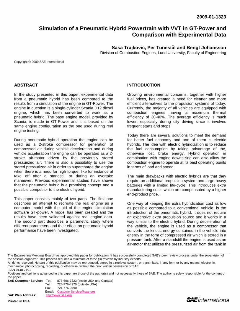
The Engineering Meetings Board has approved this paper for publication. It has successfully completed SAE’s peer review process under the supervision of the session organizer. This process requires a minimum of three (3) reviews by industry experts. All rights reserved. No part of this publication may be reproduced, stored in a retrieval system, or transmitted, in any form or by any means, electronic, mechanical, photocopying, recording, or otherwise, without the prior written permission of SAE. ISSN 0148-7191 Positions and opinions advanced in this paper are those of the author(s) and not necessarily those of SAE. The author is solely responsible for the content of the paper. SAE Customer Service: Tel: 877-606-7323 (inside USA and Canada) Tel: 724-776-4970 (outside USA) Fax: 724-776-0790 Email: [email protected] SAE Web Address: http://www.sae.org
Printed in USA
2009-01-1323
Simulation of a Pneumatic Hybrid Powertrain with VVT in GT-Power and Comparison with Experimental Data
Sasa Trajkovic, Per Tunestål and Bengt Johansson Division of Combustion Engines, Lund University, Faculty of Engineering
Copyright © 2009 SAE International
ABSTRACT
In the study presented in this paper, experimental data from a pneumatic hybrid has been compared to the results from a simulation of the engine in GT-Power. The engine in question is a single-cylinder Scania D12 diesel engine, which has been converted to work as a pneumatic hybrid. The base engine model, provided by Scania, is made in GT-Power and it is based on the same engine configuration as the one used during real engine testing.
During pneumatic hybrid operation the engine can be used as a 2-stroke compressor for generation of compressed air during vehicle deceleration and during vehicle acceleration the engine can be operated as a 2-stroke air-motor driven by the previously stored pressurized air. There is also a possibility to use the stored pressurized air in order to supercharge the engine when there is a need for high torque, like for instance at take off after a standstill or during an overtake maneuver. Previous experimental studies have shown that the pneumatic hybrid is a promising concept and a possible competitor to the electric hybrid.
This paper consists mainly of two parts. The first one describes an attempt to recreate the real engine as a computer model with the aid of the engine simulation software GT-power. A model has been created and the results have been validated against real engine data. The second part describes a parametric study where different parameters and their effect on pneumatic hybrid performance have been investigated.
INTRODUCTION
Growing environmental concerns, together with higher fuel prices, has created a need for cleaner and more efficient alternatives to the propulsion systems of today. Currently, the majority of all vehicles are equipped with combustion engines having a maximum thermal efficiency of 30-40%. The average efficiency is much lower, especially during city driving since it involves frequent starts and stops.
Today there are several solutions to meet the demand for better fuel economy and one of them is electric hybrids. The idea with electric hybridization is to reduce the fuel consumption by taking advantage of the, otherwise lost, brake energy. Hybrid operation in combination with engine downsizing can also allow the combustion engine to operate at its best operating points in terms of load and speed.
The main drawbacks with electric hybrids are that they require an additional propulsion system and large heavy batteries with a limited life-cycle. This introduces extra manufacturing costs which are compensated by a higher end-product price.
One way of keeping the extra hybridization cost as low as possible compared to a conventional vehicle, is the introduction of the pneumatic hybrid. It does not require an expensive extra propulsion source and it works in a way similar to the electric hybrid. During deceleration of the vehicle, the engine is used as a compressor that converts the kinetic energy contained in the vehicle into energy in the form of compressed air which is stored in a pressure tank. After a standstill the engine is used as an air-motor that utilizes the pressurized air from the tank in

order to accelerate the vehicle. During a full stop the engine can be shut off.
In this study, a model of the pneumatic hybrid engine has been created with the intent to further explore its potential and characteristics. Previous experimental studies [1, 2] have shown that different factors, like for instance tank valve head diameter and valve timings, play an important role in the overall pneumatic hybrid performance. While it is time consuming to change the tank valve head diameter on a real engine, it can be done within seconds on a computer model. Therefore a real engine based computer model can serve as a tool in order to more easily find optimal engine parameters.
PNEUMATIC HYBRID
Pneumatic hybrid operation introduces new operating modes in addition to conventional internal combustion engine (ICE) operation. The main idea with pneumatic hybrid is to use the ICE in order to compress atmospheric air and store it in a pressure tank when decelerating the vehicle. The stored compressed air can then be used either to accelerate the vehicle or to supercharge the engine in order to achieve higher loads when needed. The pneumatic hybrid also makes it possible to completely shut off the engine at idling like for instance at a stoplight, which in turn contributes to lower fuel consumption. [3,4,5,6]
In this study a single-cylinder engine was used. In reality, in for instance a heavy duty truck, one cylinder will not be enough to take full advantage of the pneumatic hybrid. A pneumatic hybrid will most probably utilize multiple cylinders. The number of cylinders that will be converted for pneumatic hybrid operation for a certain vehicle is hard to estimate at this point. It depends on, among other things, the vehicle weight and the maximum braking torque needed.
MODES OF ENGINE OPERATION
The main pneumatic hybrid vehicle operations are compressor mode (CM) and air-motor mode (AM).
COMPRESSOR MODE
In compressor mode (CM) the engine is used as a 2-stroke compressor in order to decelerate the vehicle. The kinetic energy of the moving vehicle is converted to potential energy in the form of compressed air.
During CM the inlet valve opens a number of crank angle degrees (CAD) after top dead centre (ATDC) and brings fresh air to the cylinder, and closes around bottom dead centre (BDC). The moving piston starts to compress the air contained in the cylinder after BDC and the tank valve opens somewhere between BDC and TDC, depending on how much braking torque is needed, and closes shortly after TDC. The compressed air
generated during CM is stored in a pressure tank that is connected to the cylinder head.
AIR-MOTOR MODE
In air-motor mode (AM) the engine is used as a 2-stroke air-motor that uses the compressed air from the pressure tank in order to accelerate the vehicle. The potential energy in the form of compressed air is converted to mechanical energy on the crankshaft which in the end is converted to kinetic energy.
During AM the tank valve opens at TDC or shortly after and the compressed air fills the cylinder to give the torque needed in order to accelerate the vehicle. Somewhere between TDC and BDC the tank valve closes, depending on how much torque the driver demands. Increasing the tank valve duration will increase the torque generated by the compressed air. The inlet valve opens around BDC in order to allow the compressed air to escape from the cylinder.
EXPERIMENTAL SETUP
The engine used in this study can be seen in Figure 1. It is a 6-cylinder Scania D12 diesel engine converted to a single-cylinder engine. The engine is equipped with a pneumatic-electric fully variable valve actuating system which has been more thoroughly described by Trajkovic et al. [7]. The geometric properties of the engine can be seen in Table 1. Figure 2 shows a close-up of the pneumatic valve actuators mounted on top of the Scania cylinder head.
Figure 1 The engine used in this study
The exhaust valves were deactivated throughout the whole study because no fuel was injected and thus there was no need for exhaust gas venting.

PRESSURE COMPENSATED TANK VALVE Table 1 Engine geometric properties
Experiments done by Trajkovic et al. [1] showed that the chosen tank valve diameter was too small and introduced unnecessary pressure losses with a reduced efficiency as a result. In an attempt to avoid these pressure losses, an in-house designed pneumatic valve spring was developed and used instead of the conventional tank valve spring. The main idea with the pneumatic valve spring was to pressure compensate the tank valve, which means that the forces, generated by the pressurized air, acting on the tank valve are cancelled out. The net force acting on the valve is therefore zero which means that the tank valve can be kept closed without using any valve spring. The valve diameter can therefore be increased in order to reduce the pressure losses over the tank valve.
Displaced Volume 1966 cm3 Bore 127.5 mm Stroke 154 mm Connecting Rod Length 255 mm Number of Valves 4 Compression Ratio 18:1 Piston type Flat Inlet valve diameter 45 mm Inlet valve diameter 41 mm Tank valve diameter 16 and 28 mm Piston clearance 7.3 mm
TANK VALVE The pneumatic valve spring arrangement requires the pneumatic valve actuators to be fed with pressurized air at the same pressure level as the cylinder pressure at the time of expected tank valve opening. Therefore, the tank valve actuator was fed with pressurized air directly from the pressure tank.
In order to run the engine as a pneumatic hybrid, a 50 litre pressure tank has to be connected to the cylinder head. Tai et al. [3] describe an intake air switching system in which one inlet valve per cylinder is fed by either fresh intake air or compressed air from the pressure tank. Andersson et al. [8] describe a dual valve system where one of the intake ports has two valves,
A more thorough and detailed description of the pneumatic valve spring arrangement and its characteristics can be found in [2].
ENGINE MODELING
The base engine model, provided by Scania, is made in GT-Power and it is based on the same base engine configuration as the one used during real engine testing. However, since only one cylinder was used during the experimental study, the base model had to be modified. The base model engine was equipped with camshaft driven valves which were replaced with a variable valve timing (VVT) system equivalent GT-Power part. A pressure tank was also added to the model and connected to one of the inlet ports of the engine. The final model can be seen in Figure 3.
The addition of new parts to the model introduces new unknown parameters such as heat transfer coefficient for the pressure tank, and friction losses in the metallic tubing connecting the pressure tank to the engine. Since these new parameters are unknown, great care has to be taken in tuning them. Therefore the model has to be validated against experimental engine data.
Figure 2 The pneumatic valve actuators mounted on the Scania cylinder head
one of which is connected to the air tank. A third solution would be to add an extra port to the cylinder head, which would be connected to the air tank. Since these three solutions demand significant modifications to a standard engine a simpler solution, where one of the existing inlet valves has been converted to a tank valve, has been chosen for this study. Since the engine used in this study has separated air inlet ports, there will be no interference between the intake system and the compressed air system. The drawback with this solution is that there will be a significant reduction in peak power, and reduced ability to generate and control swirl for good combustion.
An important aspect of model validation is that the relative error between measured data and simulated data should not exceed a certain value in order to name the model “reliable”. Morrissey et al. [9] showed results where the error ranges up to 30% while Westin et al. [10] showed steady-state operating points with an inaccuracy of 5-10%. The aim of the model calibration in this study was to ensure that the error would not exceed 5% for as many model parameters as possible.
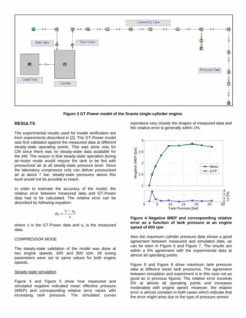
Figure 3 GT-Power model of the Scania single-cylinder engine.
RESULTS
The experimental results used for model verification are from experiments described in [2]. The GT-Power model was first validated against the measured data at different steady-state operating points. This was done only for CM since there was no steady-state data available for the AM. The reason is that steady-state operation during air-motor mode would require the tank to be fed with pressurized air at all steady-state pressure level. Since the laboratory compressor only can deliver pressurized air at about 7 bar, steady-state pressures above this level would not be possible to reach.
In order to estimate the accuracy of the model, the relative error between measured data and GT-Power data had to be calculated. The relative error can be described by following equation:
where x is the GT-Power data and x0 is the measured data.
COMPRESSOR MODE
The steady-state validation of the model was done at two engine speeds, 600 and 900 rpm. All tuning parameters were set to same values for both engine speeds.
Steady-state simulation
Figure 4 and Figure 5 show how measured and simulated negative indicated mean effective pressure (IMEP) and corresponding relative error varies with increasing tank pressure. The simulated curves
reproduce very closely the shapes of measured data and the relative error is generally within 1%.
Figure 4 Negative IMEP and corresponding relative error as a function of tank pressure at an engine speed of 600 rpm
Also the maximum cylinder pressure data shows a good agreement between measured and simulated data, as can be seen in Figure 6 and Figure 7. The results are within a 5% agreement with the experimental data at almost all operating points.
Figure 8 and Figure 9 show maximum tank pressure data at different mean tank pressures. The agreement between simulation and experiment is in this case not as good as in previous figures. The relative error exceeds 5% at almost all operating points and increases moderately with engine speed. However, the relative error is almost constant in both cases which indicate that the error might arise due to the type of pressure sensor
1
1.5
2
2.5
3
Ne
ga
tive
IME
P [b
ar]
MeasGTP
0 5 10 15 20 25 300123
Tank Pressure [bar]
δx [%
]

Figure 5 Negative IMEP and corresponding relative error as a function of tank pressure at an engine speed of 900 rpm
Figure 6 Maximum cylinder pressure and corresponding relative error as a function of tank pressure at an engine speed of 600 rpm
used to measure the port pressure. The sensor in question is a piezoresistive transducer and according to tests done by Tsung et al. [11] the response rate of such transducers are one quarter of the response rate of piezoelectric transducers usually used for in-cylinder pressure measurement. This means that the pressure signal achieved with the piezoresistive transducer is damped and therefore deviates from what would be achieved with a piezoelectric transducer.
The tank valve port temperature can be seen in Figure 10 and Figure 11. The relative error reaches almost 10% at some point which implies that additional calibration needs to be done in order to achieve satisfactory results. The reason why predicted results deviates heavily from measured is that the calibration has mainly been focused on setting the right dimensions of the pipes and connections rather than tuning the heat transfer coefficients and wall temperatures. A greater care in
Figure 7 Maximum cylinder pressure and corresponding relative error as a function of tank pressure at an engine speed of 900 rpm
Figure 8 Maximum tank pressure together with the corresponding relative error at 600 rpm
Figure 9 Maximum tank pressure together with the corresponding relative error at 900 rpm
1
1.5
2
2.5
3
3.5N
eg
ativ
e IM
EP
[ba
r]
MeasGTP
0 5 10 15 20 25 30-2024
Tank Pressure [bar]
δx [%
]
0
5
10
15
20
25
Ma
x C
ylin
de
r P
ress
ure
[ba
r]
MeasGTP
0 5 10 15 20 25 300
5
Tank Pressure [bar]
δx [%
]
0
5
10
15
20
25
Ma
x C
ylin
de
r P
ress
ure
[ba
r]
MeasGTP
0 5 10 15 20 25 300510
Tank Pressure [bar]
δx [%
]
0
5
10
15
20
25
Ma
x T
an
k P
ress
ure
[ba
r]
MeasGTP
0 5 10 15 20 25 300
5
10
Tank Pressure [bar]
δx [%
]
0
5
10
15
20
25
Ma
x T
an
k P
ress
ure
[ba
r]
MeasGTP
0 5 10 15 20 25 30
6810
Tank Pressure [bar]
δx [%
]

calibration of these parameters would most likely decrease the margin of error. The decline in temperature for the simulated data between tank pressures of 15 and 25 bar indicates that the heat losses in the model are greater compared to measured data.
Transient simulation
During transient engine operation, the valve timings of both the intake and the tank valve are open-loop controlled. The valve timing map has been created from data retrieved during steady-state operation.
Figure 10 Tank valve port temperature and corresponding relative error as a function of tank pressure at an engine speed of 600 rpm
Figure 11 Tank valve port temperature and corresponding relative error as a function of tank pressure at an engine speed of 900 rpm
Figure 12 and Figure 13 show negative IMEP during 800 consecutive cycles of transient engine operation for both simulated and measured values. The agreement of simulated data with measured data is quite good with a relative error mainly within 5 %. However, between 0
and 200 engine cycles, the error exceeds 5 % for both cases. It is difficult to estimate exactly why the simulated data deviates in this way, but one explanation might be poor tuning with respect to heat transfer. The hump-like behavior in Figure 13 in the cycle-interval of 100-200 cycles occurs due to some issues with the pneumatic valve spring arrangement. These issues have been thoroughly discussed in [2]. A behavior like this is quite hard to simulate and therefore there will be some discrepancy between measured and predicted values.
If the results from transient operation are compared with
Figure 12 Negative IMEP and corresponding relative error as a function of engine cycle number during transient CM simulation at an engine speed of 600 rpm
Figure 13 Negative IMEP and corresponding relative error as a function of engine cycle number during transient CM simulation at an engine speed of 900 rpm
those retrieved during steady-state simulations, it can be noticed that transient operation lead to a higher relative error. There might be various possible reasons for such behavior. The most probable reason is that transient gas
350
400
450
500
550
Ta
nk
Va
lve
Po
rt T
em
pe
ratu
re [K
]
MeasGTP
0 5 10 15 20 25 30-10
0
10
Tank Pressure [bar]
δx [%
]
350
400
450
500
550
600
650
Ta
nk
Va
lve
Po
rt T
em
pe
ratu
re [K
]
MeasGTP
0 5 10 15 20 25 30-10
-5
0
Tank Pressure [bar]
δx [%
]
0
1
2
3
4
Ne
ga
tive
IME
P [b
ar]
MeasGTP
0 200 400 600 800-5
0
5
Number of Engine Cycles
δx [%
]0
1
2
3
4
Ne
ga
tive
IME
P [b
ar]
MeasGTP
0 200 400 600 800-5
0
5
Number of Engine Cycles
δx [%
]
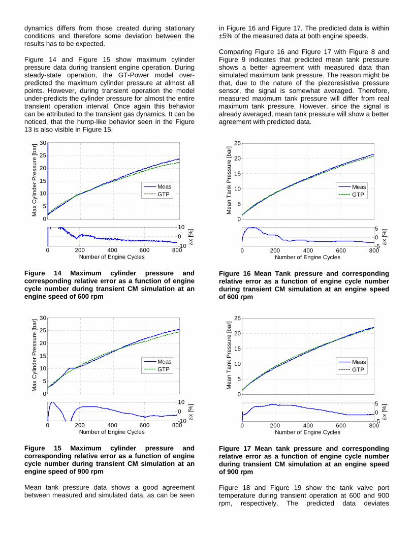
dynamics differs from those created during stationary conditions and therefore some deviation between the results has to be expected.
Figure 14 and Figure 15 show maximum cylinder pressure data during transient engine operation. During steady-state operation, the GT-Power model over-predicted the maximum cylinder pressure at almost all points. However, during transient operation the model under-predicts the cylinder pressure for almost the entire transient operation interval. Once again this behavior can be attributed to the transient gas dynamics. It can be noticed, that the hump-like behavior seen in the Figure 13 is also visible in Figure 15.
Figure 14 Maximum cylinder pressure and corresponding relative error as a function of engine cycle number during transient CM simulation at an engine speed of 600 rpm
Figure 15 Maximum cylinder pressure and corresponding relative error as a function of engine cycle number during transient CM simulation at an engine speed of 900 rpm
Mean tank pressure data shows a good agreement between measured and simulated data, as can be seen
in Figure 16 and Figure 17. The predicted data is within ±5% of the measured data at both engine speeds.
Comparing Figure 16 and Figure 17 with Figure 8 and Figure 9 indicates that predicted mean tank pressure shows a better agreement with measured data than simulated maximum tank pressure. The reason might be that, due to the nature of the piezoresistive pressure sensor, the signal is somewhat averaged. Therefore, measured maximum tank pressure will differ from real maximum tank pressure. However, since the signal is already averaged, mean tank pressure will show a better agreement with predicted data.
Figure 16 Mean Tank pressure and corresponding relative error as a function of engine cycle number during transient CM simulation at an engine speed of 600 rpm
Figure 17 Mean tank pressure and corresponding relative error as a function of engine cycle number during transient CM simulation at an engine speed of 900 rpm
Figure 18 and Figure 19 show the tank valve port temperature during transient operation at 600 and 900 rpm, respectively. The predicted data deviates
0
5
10
15
20
25
30
Ma
x C
ylin
de
r P
ress
ure
[ba
r]
MeasGTP
0 200 400 600 800-10
0
10
Number of Engine Cycles
δx [%
]
0
5
10
15
20
25
30
Ma
x C
ylin
de
r P
ress
ure
[ba
r]
MeasGTP
0 200 400 600 800-10
0
10
Number of Engine Cycles
δx [%
]
0
5
10
15
20
25
Me
an
Ta
nk
Pre
ssu
re [b
ar]
MeasGTP
0 200 400 600 800-5
0
5
Number of Engine Cycles
δx [%
]
0
5
10
15
20
25
Me
an
Ta
nk
Pre
ssu
re [b
ar]
MeasGTP
0 200 400 600 800-5
0
5
Number of Engine Cycles
δx [%
]

considerably at some points during transient operation, comparable with the results from steady-state operation. It can be noticed that the starting temperature in both figures are not the same for measured data compared to simulated data. These results support the need for additional calibration of heat transfer related parameters.
Figure 18 Tank valve port temperature and corresponding relative error as a function of engine cycle number during transient CM simulation at an engine speed of 600 rpm
Figure 19 Tank valve port temperature and corresponding relative error as a function of engine cycle number during transient CM simulation at an engine speed of 900 rpm
AIR-MOTOR MODE
As stated before, measured steady-state data from AM operation are not available due to a limited supply of pressurized air at pressure levels exceeding 7 bar. Therefore, this subsection deals only with results retrieved from transient AM operation. All AM results have been achieved at an engine speed of 600 rpm.
Transient simulation
Figure 20 shows positive IMEP created during 800 consecutive cycles of transient AM operation for both simulated and measured values. The simulated curve reproduces the shape of the measured data very well with a relative error mainly within 5 %.
Figure 20 Positive IMEP and corresponding relative error as a function of engine cycle number during transient AM simulation
Figure 21 Maximum cylinder pressure and corresponding relative error as a function of engine cycle number during transient AM simulation
In Figure 21, simulated and measured maximum cylinder pressure can be seen. In this case, the relative error is very large and at some points it exceeds 100%. This means that greater care regarding calibration has to be taken. The offset between measured and simulated data are almost constant throughout the whole transient interval. The reason for occurrence of this offset is that the valve lift profiles for experimental and predicted data differs from one another, which can be seen in Figure 22. The simulated tank valve lift goes from minimum to maximum almost instantly, while it takes about 70 CAD
350
400
450
500
550
600
Ta
nk
Va
lve
Po
rt T
em
pe
ratu
re [K
]
MeasGTP
0 200 400 600 800-10
0
10
Number of Engine Cycles
δx [%
]
350
400
450
500
550
600
Ta
nk
Va
lve
Po
rt T
em
pe
ratu
re [ o C
]
MeasGTP
0 200 400 600 800-10
0
10
Number of Engine Cycles
δx [%
]
0
1
2
3
4
Po
sitiv
e IM
EP
[ba
r]
MeasGTP
0 100 200 300 400 500-10
0
10
Number of Engine Cycles
δx [%
]
0
5
10
15
20
25
Ma
x C
ylin
de
r P
ress
ure
[ba
r]
MeasGTP
0 100 200 300 400 5000
50
100
Number of Engine Cyclesδx
[%]

for the measured valve lift to do the same. This means that the flow into the cylinder will reach a maximum much faster with the simulated valve lift compared to the measured valve lift. This sudden state of maximal flow area will lead to the generation of a pressure wave which will propagate through the cylinder and contribute to an abrupt increase in cylinder pressure. In the case with measured valve lift, the filling of the cylinder will be smoother and therefore the maximum cylinder pressure will be lower compared to the simulated valve lift. To get rid of this problem, the measured valve lift curves should be implemented in the GT-Power model.
Figure 22 Tank valve lift profiles, measured and simulated.
Figure 23 Mean tank pressure and corresponding relative error as a function of engine cycle number during transient AM simulation
Figure 23 shows the mean tank pressure during transient AM operation. The relative error in this case ranges from 5 to 40%. In spite of this, it can be noticed that the simulated results follow the trend of the measured results. The poor agreement between predicted and measured data can be explained with references to Figure 24 which shows the tank valve port temperature. It is quite clear from Figure 24 that the
initial temperature is not calibrated well. The difference in incline between measured and predicted data indicates that the heat transfer needs additional tuning. These inclines in temperature means that the pressure in the tank will decrease, not only because it is used for motoring the engine, but also because of cooling of the hot pressurized air. Since the temperature is decreasing at a higher rate for the measured data compared to simulated, the tank pressure will do the same and this is the reason why the simulated tank pressure is higher than the measured pressure at all time during transient AM operation.
Figure 24 Tank valve port temperature and corresponding relative error as a function of engine cycle number during transient AM simulation
PARAMETRIC STUDY
The aim with this parametric study is to investigate the effects of different parameters on the pneumatic hybrid performance. The following parameters are considered in this study: Tank valve opening (TankVO), Tank valve diameter and tank hose length. The results will be thoroughly discussed below.
Since simulation of AM shows that additional calibration is crucial for predictive accuracy, the parametric study will only focus on CM.
TankVO sweep
Proper TankVO timing is crucial regarding pneumatic hybrid performance. For optimal CM efficiency the tank valve should open when the tank pressure equals the cylinder pressure. A premature TankVO, leads to a blowdown of compressed air into the cylinder with a decrease in pneumatic hybrid efficiency, as a result. A late TankVO will lead to an overshoot in cylinder pressure compared to the tank pressure and CM efficiency will suffer. However, at some situations the maximum achievable braking torque is more important than the efficiency.
-150 -100 -50 0 50 100 1500
1
2
3
4
5
6
7
8
CAD [ATDC]
Ta
nk
Va
lve
Lift
[mm
]
MeasGTP
0
5
10
15
20
25
Me
an
Ta
nk
Pre
ssu
re [b
ar]
MeasGTP
0 100 200 300 400 50002040
Number of Engine Cycles
δx [%
]
300
350
400
450
500
550
Ta
nk
Va
lve
Po
rt T
em
pe
ratu
re [K
]
MeasGTP
0 100 200 300 400 500-40
-20
0
Number of Engine Cycles
δx [%
]

Figure 25 illustrates a TankVO sweep for various steady-state tank pressures at an engine speed of 600 and 900 rpm, respectively. It can clearly be seen how negative IMEP is affected by TankVO timing. The figure shows that there is an optimal TankVO timing for every tank pressure when taking highest efficiency into consideration, where highest efficiency occurs near the minimum in each IMEP curve. This means that it takes less power to compress the inducted air at this point than at any other point on the curve at a given tank pressure. The results indicate that higher negative IMEP and thus braking torque is achieved with early TankVO. The braking torque at a TankVO of 180 CAD before TDC (BTDC) is quite impressive, see Figure 26. According to [12], the exhaust brake of a Scania 16-litre engine produces up to 3000 Nm of torque. The maximum break
Figure 25 Negative IMEP obtained during steady-state CM as a function of TankVO at various tank pressures for engine speeds of 600 and 900 rpm
Figure 26 Engine torque obtained during steady-state CM as a function of TankVO at various tank pressures at an engine speed of 600 rpm
torque during CM at 12 bar of tank pressure reaches 400 Nm for a 2-litre cylinder given in 2-stroke scale. This
means that a 16-litre engine would produce 6400 Nm in 4-stroke scale.
Tank Valve Diameter sweep
In a previous study done by Trajkovic et al. [2] results retrieved with two different tank valve geometries were compared. The results indicated that an increase in tank valve diameter from 16 mm to 28 mm reduces the pressure drop over the tank valve, contributing to higher pneumatic hybrid efficiency.
Changing valve geometries on an experimental engine is very time consuming since both the original valve and corresponding valve seating has to be modified. Such modification can often only be done by specialized workshops, which further prolongs lead time between valve changes. With a GT-Power model, a change in valve diameter can be done within seconds, hence making it a very powerful and time saving tool for optimization purposes.
Figure 27 Cylinder pressure obtained during steady-state CM for various tank valve diameters at a tank pressure of about 9.5 bar
Figure 27 shows how cylinder pressure varies with tank valve diameter during steady-state CM operation. The results indicate that the biggest difference lies in the interval of 10-20 mm in valve diameter. Figure 28 shows a 3D-view of the results shown in Figure 27. It can clearly be seen that there is almost no difference in cylinder pressure in the interval of 20-45 mm in valve diameter. This means that as long as the valve diameter is above a threshold value, in this case 20 mm, the change in CM efficiency will be modest.
The same line of argument as with previous two figures can be applied to Figure 29. With a tank valve diameter of 10 mm, the flow into the tank is limited and results in a high in-cylinder pressure and IMEP. As the valve diameter increases, IMEP decreases to a point where an increase in diameter no longer has any effect on IMEP.
-200 -150 -100 -50 00
2
4
6
8
10
12
14
TankVO [CAD BTDC]
Ne
ga
tive
IME
P [b
ar]
4 bar, 600 rpm4 bar, 900 rpm8 bar, 600 rpm8 bar, 900 rpm12 bar, 600 rpm12 bar, 900 rpm
-200 -150 -100 -50 050
100
150
200
250
300
350
400
450
TankVO [CAD BTDC]
En
gin
e T
orq
ue
[Nm
]
4 bar8 bar12 bar
-50 0 500
5
10
15
20
25
CAD [ATDC]
Cyl
ind
er
Pre
ssu
re [b
ar]
∅=10 mm∅=20 mm∅=30 mm∅=40 mm

Figure 28 A 3D-view of cylinder pressure during steady-state CM operation for various tank valve diameters at a tank pressure of about 9.5 bar
Figure 29 Negative IMEP obtained during steady-state CM as a function of tank pressure at various tank valve diameters
The effects of various tank valve diameters on CM have also been investigated during transient CM operation. Figure 30 illustrates how IMEP varies during 800 consecutive cycles. The results show a similar trend as seen previously in Figure 29. In Figure 31 the corresponding mean tank pressure can be seen. The tank pressure at a tank valve diameter of 10 mm is much lower compared to all the remaining cases. This proves that the air flow into the tank is restricted and thus the tank will be charged with a smaller amount of pressurized air. With valve diameters larger than 10 mm, almost no difference can be noticed in tank pressure.
Tank hose length sweep
It is widely known that the geometry of the intake and exhaust lines has a great influence on the gas wave motion, which can be utilized for supercharging of the
Figure 30 Negative IMEP obtained during transient CM operation as a function of engine cycle number at various tank valve diameters
Figure 31 Tank pressure obtained during transient CM operation as a function of engine cycle number at various tank valve diameters
engine. Knowledge of pressure wave propagation is also important for the pneumatic hybrid. If the pipeline connecting the pressure tank to the engine is poorly tuned, a pressure wave can propagate back into the cylinder while the tank valve is open which can lead to a less than optimal charging of the tank.
Figure 32 shows how cylinder pressure varies with tank hose length. It can clearly be seen that all pressure curves differs from one another, which indicates that the length of the pipes indeed has a considerable effect on the wave motion. This can also be verified with references to Figure 33, which shows a 3D-view of the results from Figure 32. The 3D-view gives a better insight into how the wave motion changes with tank hose length.
In Figure 34, negative IMEP as a function of tank pressure for various tank hose lengths can be seen. The
0 5 10 15 20 25 300.5
1
1.5
2
2.5
3
3.5
Tank Pressure [bar]
Ne
ga
tive
IME
P [b
ar]
∅=10 mm∅=15 mm∅=20 mm∅=25 mm∅=30 mm∅=35 mm∅=40 mm∅=45 mm
0 200 400 600 8000.5
1
1.5
2
2.5
3
Number of Engine Cycles [bar]
Ne
ga
tive
IME
P [b
ar]
∅=10 mm∅=20 mm∅=30 mm∅=40 mm
0 200 400 600 8000
5
10
15
20
25
Number of Engine Cycles [bar]
Ta
nk
Pre
ssu
re [b
ar]
∅=10 mm∅=20 mm∅=30 mm∅=40 mm
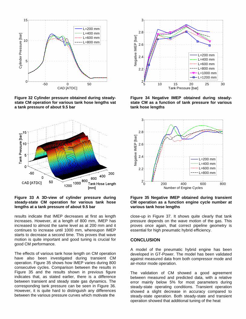
Figure 32 Cylinder pressure obtained during steady-state CM operation for various tank hose lengths vat a tank pressure of about 9.5 bar
Figure 33 A 3D-view of cylinder pressure during steady-state CM operation for various tank hose lengths at a tank pressure of about 9.5 bar
results indicate that IMEP decreases at first as length increases. However, at a length of 800 mm, IMEP has increased to almost the same level as at 200 mm and it continues to increase until 1000 mm, whereupon IMEP starts to decrease a second time. This proves that wave motion is quite important and good tuning is crucial for good CM performance.
The effects of various tank hose length on CM operation have also been investigated during transient CM operation. Figure 35 shows how IMEP varies during 800 consecutive cycles. Comparison between the results in Figure 35 and the results shown in previous figure indicates that, as stated earlier, there is a difference between transient and steady state gas dynamics. The corresponding tank pressure can be seen in Figure 36. However, it is quite hard to distinguish any differences between the various pressure curves which motivate the
Figure 34 Negative IMEP obtained during steady-state CM as a function of tank pressure for various tank hose lengths
Figure 35 Negative IMEP obtained during transient CM operation as a function engine cycle number at various tank hose lengths
close-up in Figure 37. It shows quite clearly that tank pressure depends on the wave motion of the gas. This proves once again, that correct pipeline geometry is essential for high pneumatic hybrid efficiency.
CONCLUSION
A model of the pneumatic hybrid engine has been developed in GT-Power. The model has been validated against measured data from both compressor mode and air-motor mode operation.
The validation of CM showed a good agreement between measured and predicted data, with a relative error mainly below 5% for most parameters during steady-state operating conditions. Transient operation showed a slight decrease in accuracy compared to steady-state operation. Both steady-state and transient operation showed that additional tuning of the heat
-50 0 500
5
10
15
CAD [ATDC]
Cyl
ind
er
Pre
ssu
re [b
ar]
L=200 mmL=400 mmL=600 mmL=800 mm
5 10 15 20 25 302
2.2
2.4
2.6
2.8
3
Tank Pressure [bar]
Ne
ga
tive
IME
P [b
ar]
L=200 mmL=400 mmL=600 mmL=800 mmL=1000 mmL=1200 mm
0 200 400 600 8002
2.2
2.4
2.6
2.8
3
Number of Engine Cycles
Ne
ga
tive
IME
P [b
ar]
L=200 mmL=400 mmL=600 mmL=800 mm

Figure 36 Tank pressure obtained during transient CM operation as a function engine cycle number at various tank hose lengths
Figure 37 Close-up of the tank pressure curves shown in Figure 36
transfer needs to be done in order to further increase the accuracy.
The agreement between predicted and measured data for AM operation was not as good as with CM operation. The uncertainty during transient operation exceeded 40% in some cases. One reason is inadequate tuning of parameters associated with heat transfer and initial wall temperatures. Another reason is that the simulated valve lift profiles did not match the corresponding measured valve lift profiles.
A parametric study was conducted, where the influence of tank valve timing, tank valve diameter and tank hose length on pneumatic hybrid performance were investigated.
The investigation of tank valve timing illustrated the effect of tank valve opening on IMEP and torque. An engine torque of 400 Nm (2-stroke) for a 2-litre cylinder was achieved at a tank pressure of 12 bar.
The search for optimal tank valve diameter showed that as long as the valve diameter is above a threshold value, in this case 20 mm, the change in CM efficiency will be modest.
It was shown that tank hose length to a great extent influences the wave motion of the gas, and therefore a great care in choosing the right pipeline geometry is essential for good pneumatic hybrid performance.
REFERENCES
1. S. Trajkovic, P. Tunestål and B. Johansson, “Introductory Study of Variable Valve Actuation for Pneumatic Hybridization”, SAE Paper 2007-01-0288, 2007
2. S. Trajkovic, P. Tunestål and B. Johansson, “Investigation of Different Valve Geometries and Valve Timing Strategies and their Effect on Regenerative Efficiency for a Pneumatic Hybrid with Variable Valve Actuation”, SAE Paper 2008-01-1715, 2008
3. C. Thai, T-C. Tsao, M. Levin, G. Barta and M. Schechter, “Using Camless Valvetrain for Air Hybrid Optimization”, SAE Paper 2003-01-0038, 2003
4. M. Schechter, “Regenerative Compression Braking – A low Cost Alternative to Electric Hybrids”, SAE Paper 2000-01-1025, 2000
5. M. Schechter, “New Cycles for Automobile Engines”,
SAE paper 1999-01-0623, 1999 6. P. Higelin, A. Charlet, Y. Chamaillard,
"Thermodynamic Simulation of a Hybrid Pneumatic-Combustion Engine Concept International Journal of Applied Thermodynamics", Vol 5, No. 1, pp 1 – 11, ISSN 1301 9724, 2002
7. S. Trajkovic, A. Milosavljevic, P. Tunestål and B. Johansson, “FPGA Controlled Pneumatic Variable Valve Actuation”, SAE Paper 2006-01-0041, 2006
8. M. Andersson, B. Johansson and A. Hultqvist, “An Air Hybrid for High Power Absorption and Discharge”, SAE paper 2005-01-2137, 2005
9. C. Morrissey and T. Shedd, “Experimental Validation of a Carburetor Model in One-Dimensional Engine Software”, SAE Paper 2008-32-0043, 2008
10. F. Westin and H.E Ångström, “Simulation of a Turbocharged SI-Engine with Two Software and Comparison with Measured Data”, SAE Paper 2003-01-3124, 2003
0 200 400 600 8000
5
10
15
20
25
Number of Engine Cycles
Ta
nk
Pre
ssu
re [b
ar]
L=200 mmL=400 mmL=600 mmL=800 mm
650 660 670 680 690 70018
18.5
19
19.5
Number of Engine Cycles
Ta
nk
Pre
ssu
re [b
ar]
L=200 mmL=400 mmL=600 mmL=800 mm

11. T.T Tsung and L.L. Han, “Evaluation of dynamic performance of pressure sensors using a pressure square-like wave generator”, Measurement Science and Technology 15, pp 1133-1139, 2004
12. Scania, “Scania launches new 16-litre V8 with outstanding performance”. Available at http://www.scania.com/news/events/archive/2000/v8/press_16033.asp, (October 9, 2008)
CONTACT
Sasa Trajkovic, PhD student, Msc M. E.
E-mail: [email protected]
Phone: +46763161804
DEFINITIONS, ACRONYMS, ABBREVIATIONS
AM: Air-motor Mode
ATDC: After Top Dead Centre
BDC: Bottom Dead Centre
BTDC: Before Top Dead Centre
CAD: Crank Angle Degree
CM: Compressor Mode
GTP: GT-Power
ICE: Internal Combustion Engines
IMEP: Indicated Mean Effective Pressure
IVC: Inlet Valve Closing
IVO: Inlet Valve Opening
TankVO: Tank Valve Opening
TankVC: Tank Valve Closing
TDC: Top Dead Centre
RPM: Revolutions Per Minute
VVT: Variable Valve Timing

Paper 4

2010-01-0825
Vehicle Driving Cycle Simulation of a Pneumatic Hybrid Bus Based on Experimental Engine Measurements
Sasa Trajkovic, Per Tunestål and Bengt Johansson Division of Combustion Engines, Lund University
This is a work of the Government of Sweden
ABSTRACT
In the study presented in this paper, a vehicle driving cycle simulation of the pneumatic hybrid has been conducted. The pneumatic hybrid powertrain has been modeled in GT-Power and validated against experimental data. The GT-Power engine model has been linked with a MATLAB/simulink vehicle model. The engine in question is a single-cylinder Scania D12 diesel engine, which has been converted to work as a pneumatic hybrid. The base engine model, provided by Scania, is made in GT-power and it is based on the same engine configuration as the one used in real engine testing.
During pneumatic hybrid operation the engine can be used as a 2-stroke compressor for generation of compressed air during vehicle deceleration and during vehicle acceleration the engine can be operated as a 2-stroke air-motor driven by the previously stored pressurized air. There is also a possibility to use the stored pressurized air in order to supercharge the engine when there is a need for high torque, like for instance at take off after a standstill or during a overtake maneuver. Previous experimental studies have shown that the pneumatic hybrid is a promising concept with great possibility for fuel consumption reduction during city-driving conditions.
Earlier studies have shown a great reduction in fuel consumption whit the pneumatic hybrid compared to conventional vehicles of today. However, most of these studies have been completely of theoretical nature. In this paper, the engine model is based on and verified against experimental data, and therefore more realistic results can be expected.
The intent with the vehicle driving cycle simulation is to investigate the potential of the pneumatic hybrid regarding reduction in fuel consumption (FC) compared to a traditional internal combustion engine (ICE) powered vehicle.
The results show that a reduction in fuel economy of up to about 30% is possible for a pneumatic hybrid bus on the Braunschweig duty cycle. The main part of this reduction comes from the stop/start functionality of the system, while regenerative braking only contributes with 8.4 % to the reduction in FC. The results also show that an amazing 87% of the braking power can be absorbed and converted to compressed air. However, only a small portion of this energy, about 20%, can be converted to positive work.
INTRODUCTION
Growing environmental concerns, together with higher fuel prices, has created a need for cleaner and more efficient alternatives to the propulsion systems of today. Currently, the majority of all vehicles are equipped with combustion engines having a maximum thermal efficiency of 30-40%. The average efficiency is much lower, especially during city driving since it involves frequent starts and stops.
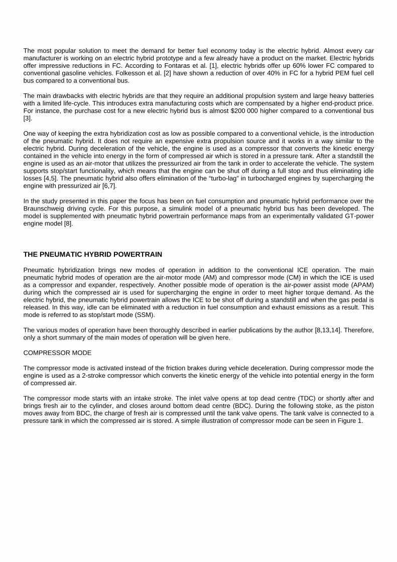
The most popular solution to meet the demand for better fuel economy today is the electric hybrid. Almost every car manufacturer is working on an electric hybrid prototype and a few already have a product on the market. Electric hybrids offer impressive reductions in FC. According to Fontaras et al. [1], electric hybrids offer up 60% lower FC compared to conventional gasoline vehicles. Folkesson et al. [2] have shown a reduction of over 40% in FC for a hybrid PEM fuel cell bus compared to a conventional bus.
The main drawbacks with electric hybrids are that they require an additional propulsion system and large heavy batteries with a limited life-cycle. This introduces extra manufacturing costs which are compensated by a higher end-product price. For instance, the purchase cost for a new electric hybrid bus is almost $200 000 higher compared to a conventional bus [3].
One way of keeping the extra hybridization cost as low as possible compared to a conventional vehicle, is the introduction of the pneumatic hybrid. It does not require an expensive extra propulsion source and it works in a way similar to the electric hybrid. During deceleration of the vehicle, the engine is used as a compressor that converts the kinetic energy contained in the vehicle into energy in the form of compressed air which is stored in a pressure tank. After a standstill the engine is used as an air-motor that utilizes the pressurized air from the tank in order to accelerate the vehicle. The system supports stop/start functionality, which means that the engine can be shut off during a full stop and thus eliminating idle losses [4,5]. The pneumatic hybrid also offers elimination of the “turbo-lag” in turbocharged engines by supercharging the engine with pressurized air [6,7].
In the study presented in this paper the focus has been on fuel consumption and pneumatic hybrid performance over the Braunschweig driving cycle. For this purpose, a simulink model of a pneumatic hybrid bus has been developed. The model is supplemented with pneumatic hybrid powertrain performance maps from an experimentally validated GT-power engine model [8].
THE PNEUMATIC HYBRID POWERTRAIN
Pneumatic hybridization brings new modes of operation in addition to the conventional ICE operation. The main pneumatic hybrid modes of operation are the air-motor mode (AM) and compressor mode (CM) in which the ICE is used as a compressor and expander, respectively. Another possible mode of operation is the air-power assist mode (APAM) during which the compressed air is used for supercharging the engine in order to meet higher torque demand. As the electric hybrid, the pneumatic hybrid powertrain allows the ICE to be shot off during a standstill and when the gas pedal is released. In this way, idle can be eliminated with a reduction in fuel consumption and exhaust emissions as a result. This mode is referred to as stop/start mode (SSM).
The various modes of operation have been thoroughly described in earlier publications by the author [8,13,14]. Therefore, only a short summary of the main modes of operation will be given here.
COMPRESSOR MODE
The compressor mode is activated instead of the friction brakes during vehicle deceleration. During compressor mode the engine is used as a 2-stroke compressor which converts the kinetic energy of the vehicle into potential energy in the form of compressed air.
The compressor mode starts with an intake stroke. The inlet valve opens at top dead centre (TDC) or shortly after and brings fresh air to the cylinder, and closes around bottom dead centre (BDC). During the following stoke, as the piston moves away from BDC, the charge of fresh air is compressed until the tank valve opens. The tank valve is connected to a pressure tank in which the compressed air is stored. A simple illustration of compressor mode can be seen in Figure 1.

Figure 1 Illustration of Compressor Mode. I) Intake of fresh air, II) Compression of air and pressure tank charging. Right port is connected to the pressure tank.
For maximum braking power, the tank valve should open in the vicinity of BDC during the compressor stroke. In this way, a specific brake torque of over 300 Nm per liter engine displacement can be achieved, as will be shown later on in this paper.
AIR-MOTOR MODE
The air-motor mode is activated during the subsequent acceleration after a standstill. During air-motor mode the engine is used as a 2-stoke air-motor/expander, converting the compressed air into kinetic energy.
The air-motor mode starts with an expansion stroke. At TDC, the tank valve opens and compressed air fills the cylinder. The closing of the valve occurs somewhere between TDC and BDC, depending on the torque demand. At BDC, the inlet valve opens and remains open during the compression stroke. The air-motor mode is illustrated in Figure 2.
Figure 2 Illustration of Air-Motor Mode. I) Intake of compressed air, II) Air venting. Right port is connected to the pressure tank.
The required amount of admitted charge into the cylinder depends on the current power demand, and is controlled by the closing point of the tank valve. For maximum AM efficiency the tank valve should close in such a way that when the piston reaches BDC, the cylinder pressure reaches atmospheric conditions. Late closing of the tank valve will lead to higher power but a low AM efficiency since the cylinder pressure at BDC will be above atmospheric conditions, with a blow down through the intake port when the inlet valve opens as a result.
VEHICLE MODELING
The base vehicle model is made in MATLAB/Simulink and is based upon a typical vehicle for personal transport and weighs 1300 kg. It is modeled with a 1.5 liter diesel engine based on maps obtained experimentally. The model has been developed by the Department of Industrial Electrical Engineering and Automation (IEA) at Lund University and has been thoroughly described in [15].

Since the purpose of the study presented in this paper was to evaluate the pneumatic hybrid powertrain implemented in a city bus, the model needed to be modified. Below, a list of the most significant modifications is presented.
The original ICE model was based on a 1.5L spark ignited (SI) 4-cylinder engine, while the city bus engine was based on a 12L direct injected (DI) 6-cylinder engine. Therefore, the original ICE model was replaced by an ICE model based on data from a GT-Power model of a SCANIA D12 engine model designed by SCANIA and validated by Svensson [16]. Geometric properties of the engine can be seen in Table 1.
All electric-hybrid related components were removed and replaced by pneumatic hybrid components. The pneumatic hybrid powertrain performance maps are generated in a GT-Power model validated against experimental data [8].
Vehicle specific data like weight, frontal area, maximum torque and power, were updated with suitable data for the chosen vehicle. The most significant vehicle data can be seen in Table 2. The auxiliary power demand of 4 kW is a mean value for the entire Braunschweig drive cycle and has been chosen in accordance with [17].
Table 1 Geometric properties of the SCANIA D12 diesel engine
Displaced Volume 1966 cm3 Bore 127.5 mm Stroke 154 mm Connecting Rod Length 255 mm Number of Valves 4 Compression Ratio 18:1 Piston type Bowl Inlet valve diameter 45 mm Exhaust valve diameter 41 mm Valve Timing Variable
Table 2 Vehicle data for the simulated city bus
Total Vehicle Weight 15000 kg Wheel Radius, rw 0.517 m Air Resistance, Cd 0.75 Rolling Resistance, Cr 0.008 Frontal Area 7.5 m2 Auxiliary power demand 4 kW Maximum Vehicle Speed 80 km/h Pressure Tank Volume 40 liter Starting tank pressure 23.7 bar Lower tank pressure limit 8 bar Upper tank pressure limit 27 bar
Figure 3 and Figure 4 show the top lever of the pneumatic hybrid bus model and the pneumatic hybrid subsystem, respectively.

Figure 3 Top level of the pneumatic hybrid bus model
Figure 4 The Pneumatic hybrid specific subsystem
THE BRAUNSCHWEIG CITY DRIVING CYCLE
To estimate the fuel saving potential of the pneumatic hybrid concept applied to a city bus, the Braunschweig cycle was used. The Braunschweig cycle was developed at the Technical University of Braunschweig, Germany and is an urban bus driving cycle with frequent stops. Figure 5 shows the vehicle speed during the entire drive cycle. The cycle contains rapid accelerations and retardations which makes it very demanding. Table 3 shows the basic parameters of the Braunschweig cycle.

Figure 5 Vehicle speed during the Braunschweig driving cycle
The reason why the Braunschweig cycle has been chosen for the study presented in this paper is that it has been frequently used in various research projects and there exists a great foundation of information which makes the validations of the model easier.
Table 3 Basic parameters of the Braunschweig cycle
Cycle Braunschweig
Time [s] 1740
Distance [km]
10.87
Av. Speed [km/h]
22.5
Max Speed [km/h] 58.2
Idle [%] 25.3
Max Acc. [m/s2]
2.41
SIMULATION RESULTS
The content of this section can be divided into three parts. In the first part, the pneumatic hybrid powertrain performance maps generated in GT-Power are discussed. The second part of this section deals with the results obtained from the vehicle simulation. Finally, in the third part, results from a study on the effect of pressure tank volume and minimum allowable tank pressure on FC will be shown.
PNEUMATIC HYBRID POWERTRAIN PERFORMANCE MAPS
In [8], a model of the pneumatic hybrid powertrain based on the SCANIA D12 engine used in this paper was developed in GT-Power and validated against experimental data. In the study presented in this paper, the same model has been used in order to create performance maps of both AM and CM. The performance maps shows the mass flow of air into or out from the tank (depending on the mode of operation) as a function of engine load and tank pressure. Figure 6 and Figure 7 show the performance map of CM while Figure 9 and Figure 10 show the performance map of AM.
From Figure 6 and Figure 7, it can be seen that, during CM operation, the engine torque and IMEP can reach very high levels. According to the Appendix the maximum achievable theoretical IMEP can be calculated with following simple equation:
0 500 1000 15000
10
20
30
40
50
60
Time [s]
Ve
hic
le S
pe
ed
[km
/h]

This mean that at a tank pressure of 20 bars and an inlet manifold pressure of 1 bar, the value of IMEP will be 19 bar. In 4-stroke scale this would correspond to 38 bar. As can be seen in Figure 7, IMEP is about 19 bar at a tank pressure of 20 bar.
Figure 6 Mass flow rate (g/cycle) in to the tank as a function of both engine torque (2-stroke scale) and tank pressure during Compressor Mode.
Figure 7 Mass flow rate (g/cycle) in to the tank as a function of both negative IMEP (2-sroke scale) and tank pressure during Compressor Mode.
The appearance of almost constant contour lines at a specific tank pressure can be explained in the following way. The charging of the tank with compressed air will not start before until the cylinder pressure and tank pressure reaches equilibrium, no matter when the tank valve opens. At higher IMEP, the tank valve will open before pressure equilibrium occurs with a blowdown of pressurized air into the cylinder, as a result, se Figure 8. The cylinder will now contain air inducted during the intake stroke and compressed air from the blowdown. As the piston approaches TDC, the air in the cylinder will be pushed into the tank and the net mass flow will only depend on the amount of air inducted during the intake stroke. This line of argument can also be illustrated by following equation:
Notice that this equation is simplified, since in reality, there will still be a portion of compressed air in the compression volume at TDC that cannot be pushed into the tank.
Tank Pressure [bar]
En
gin
e T
orq
ue
[Nm
]
1.8
1.61.4 1.2 1
0.8
5 10 15 20
100
200
300
400
500
600
700
Tank Pressure [bar]
Ne
ga
tive
IME
P [b
ar]
1.8
1.61.4 1.2 1 0.8
5 10 15 20
5
10
15
20

Figure 8 Illustration of blowdown of compressed air from the tank into the cylinder at an early tank valve opening.
Another thing that can be observed in Figure 6 is that the maximum engine brake torque at low tank pressure is very limited. This means that in order to always have access to sufficient brake torque and avoid unnecessary friction brake usage, the pressure level in the tank has to be above a threshold value. The effect of minimum allowable tank pressure will be presented later on in this paper.
The reason why mass flow rate into the tank decreases with increasing tank pressure, can be explained by two phenomena. The first is that with higher tank pressures the flow over the valve is limited due to chocking, which results in a smaller dose of compressed air pushed into the tank. The other is that at a higher tank pressure the equilibrium pressure level, at which the tank valve should open, occurs later in the compression stroke with less time to vent the cylinder from compressed air, as a result.
Figure 9 Mass flow rate (g/cycle) out from the tank as a function of both engine torque and tank pressure during Air-Motor Mode.
Tank Pressure [bar]
En
gin
e T
orq
ue
[Nm
]
2
4
6
8
10
5 10 15 20
50
100
150
200
250

Figure 10 Mass flow rate (g/cycle) out from the tank as a function of both positive IMEP and tank pressure during Air-Motor Mode.
From Figure 9 and Figure 10, it can be seen that the maximum engine load in AM is limited to about 300 Nm, which is much lower compared to maximum engine load in CM. The reason is not that it is not possible to achieve higher engine loads; according to APPENDIX A, AM has the same potential in maximum torque as CM. The problem is that AM efficiency drops rapidly with increasing load; the higher the load, the higher the required amount of compressed air becomes. This in turn means that the tank valve closing will occur much later in the cycle compared to optimal closing. This results in that the cylinder pressure level at the time of inlet valve opening (around BDC), will be higher compared to the inlet manifold pressure. Therefore, there will be a blowdown of compressed air into the intake manifold, without any positive work being extracted from it, with a decrease in AM efficiency, as a result. This behavior is confirmed by Figure 11, where a PV-diagram of one cycle during AM can be seen. The illustrated operating point corresponds to the upper right corner of Figure 9 and Figure 10. At inlet valve opening (point 3), the cylinder pressure is about 6 bar and reaches almost 1 bar at inlet valve closing (point 4). This is a pressure loss of about 5 bar, which corresponds to a energy loss of approximately 1 kJ per cycle.
Figure 11 PV-diagram of one cycle during Air-Motor Mode illustrating the blowdown of compressed air through the inlet port at high engine loads.
DRIVE CYCLE SIMULATION RESULTS
As discussed earlier in the paper, the Braunschweig drive cycle has been chosen for the drive cycle simulation for the study presented in this paper.
Tank Pressure [bar]
Po
sitiv
e IM
EP
[ba
r]
2
4
6
8
10
5 10 15 20
1
2
3
4
5
6
7
8
9
0 0.5 1 1.5 2 2.50
5
10
15
20
25
Cylinder Volume [liter]
Cyl
ind
er
Pre
ssu
re [b
ar]
Torque = 250 NmIMEP = 8.5 barTankPressure = 17.4 bar
4
3
21

Figure 12 shows how tank pressure varies during the Braunschweig drive cycle. It can be noticed that the minimum tank pressure is limited to 8 bar. According to the forthcoming sub-section, 8 bar is the lower pressure limit at which minimum FC can be observed. The underlying factors influencing this limit will be discussed more thoroughly later on in the paper.
Figure 12 Tank pressure as a function of time during the Braunschweig drive cycle
It can also be seen that the tank pressure has an upper limit at 27 bar. This limit is not chosen based on minimum FC, but rather as a safety precaution to avoid failure of pressure sensitive system components which has been experienced during the work described in [14]. In a real application this could be achieved in two ways. The first solution is the implementation of a relief valve to the system. The relief valve can then be preset to a suitable pressure at which the valve opens to release excess pressurized air to the atmosphere. The second solution is to modify the valve operation during CM. In ordinary CM operation, the intake vale opens during the expansion stroke in order to avoid generation of vacuum and to bring fresh air into the cylinder. If the pressure in the tank reaches maximum limit, the flow of fresh air into the cylinder should be avoided. Therefore, the inlet vale should be deactivated at this point. This will lead to vacuum generation during the expansion stroke followed by an induction of pressurized air from the tank and into the cylinder. The CM cycle is finished by the charging of the tank with the same air that was previously inducted into the cylinder. In this way, there will be no addition of fresh air, and the tank pressure will therefore remain constant. The second solution is probably more attractive, due to the fact that the first solution would generate unnecessary noise when releasing the surplus of compressed air.
The initial tank pressure was set to the value obtained at the end of the driving cycle. In this way, the influence of starting tank pressure on pneumatic hybrid performance was eliminated. If, for instance, the initial tank pressure would have been set to a pressure lower than the pressure at the end of the cycle, the pneumatic hybrid efficiency would have been affected negatively, due to the fact that the last portion of captured and stored braking energy would never have been used.
Table 4 Fuel consumption and energy flow parameters for a bus driving the Braunschweig duty cycle
Fuel energy used [MJ] 181.0
Road Load energy [MJ] 45.7
Braking energy [MJ] 29.1
FC with friction braking [l/100 km] 41.7
FC with Regenerative efficiency of 100% [l/100 km]
15.1
FC reduction with Regenerative efficiency of 100 % [%]
63.7
Table 4 shows the fuel consumption and energy flow for a conventional bus driving the Braunschweig duty cycle. It also presents the fuel consumption for a bus with ideal regenerative braking i.e. without any losses. The fuel consumption of
0 500 1000 15005
10
15
20
25
30
Time [s]
Ta
nk
Pre
ssu
re [b
ar]
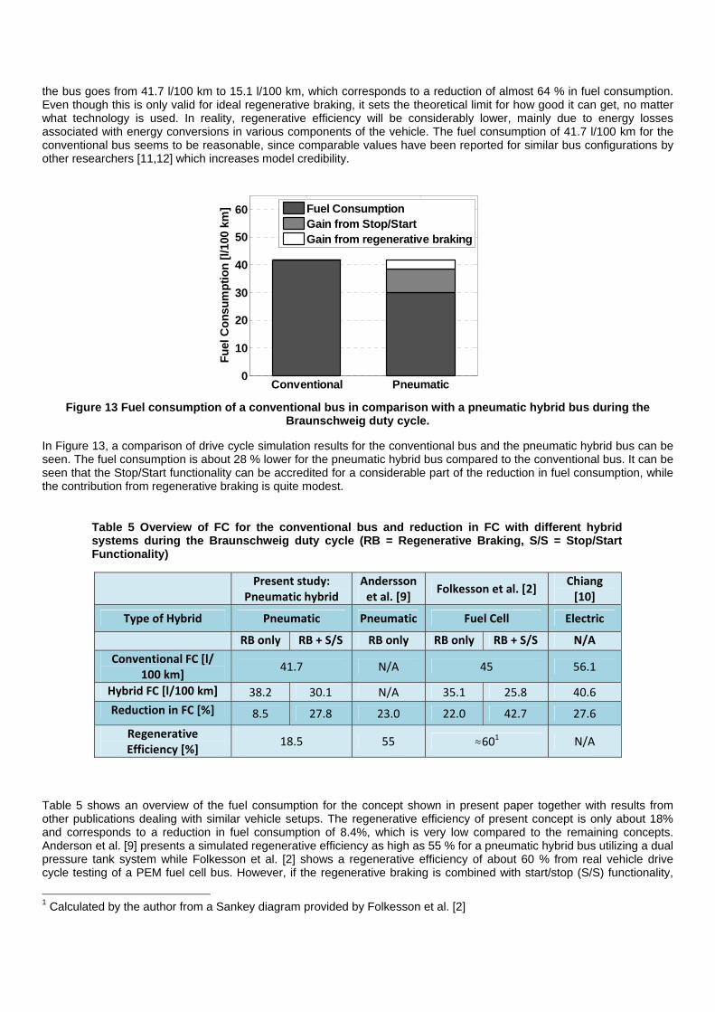
the bus goes from 41.7 l/100 km to 15.1 l/100 km, which corresponds to a reduction of almost 64 % in fuel consumption. Even though this is only valid for ideal regenerative braking, it sets the theoretical limit for how good it can get, no matter what technology is used. In reality, regenerative efficiency will be considerably lower, mainly due to energy losses associated with energy conversions in various components of the vehicle. The fuel consumption of 41.7 l/100 km for the conventional bus seems to be reasonable, since comparable values have been reported for similar bus configurations by other researchers [11,12] which increases model credibility.
Figure 13 Fuel consumption of a conventional bus in comparison with a pneumatic hybrid bus during the
Braunschweig duty cycle.
In Figure 13, a comparison of drive cycle simulation results for the conventional bus and the pneumatic hybrid bus can be seen. The fuel consumption is about 28 % lower for the pneumatic hybrid bus compared to the conventional bus. It can be seen that the Stop/Start functionality can be accredited for a considerable part of the reduction in fuel consumption, while the contribution from regenerative braking is quite modest.
Table 5 Overview of FC for the conventional bus and reduction in FC with different hybrid systems during the Braunschweig duty cycle (RB = Regenerative Braking, S/S = Stop/Start Functionality)
Present study: Pneumatic hybrid
Andersson et al. [9]
Folkesson et al. [2] Chiang [10]
Type of Hybrid Pneumatic Pneumatic Fuel Cell Electric
RB only RB + S/S RB only RB only RB + S/S N/A
Conventional FC [l/ 100 km]
41.7 N/A 45 56.1
Hybrid FC [l/100 km] 38.2 30.1 N/A 35.1 25.8 40.6
Reduction in FC [%] 8.5 27.8 23.0 22.0 42.7 27.6
Regenerative Efficiency [%]
18.5 55 ≈601 N/A
Table 5 shows an overview of the fuel consumption for the concept shown in present paper together with results from other publications dealing with similar vehicle setups. The regenerative efficiency of present concept is only about 18% and corresponds to a reduction in fuel consumption of 8.4%, which is very low compared to the remaining concepts. Anderson et al. [9] presents a simulated regenerative efficiency as high as 55 % for a pneumatic hybrid bus utilizing a dual pressure tank system while Folkesson et al. [2] shows a regenerative efficiency of about 60 % from real vehicle drive cycle testing of a PEM fuel cell bus. However, if the regenerative braking is combined with start/stop (S/S) functionality,
1 Calculated by the author from a Sankey diagram provided by Folkesson et al. [2]
Conventional Pneumatic0
10
20
30
40
50
60F
uel
Co
nsu
mp
tio
n [
l/100
km
]
Fuel ConsumptionGain from Stop/StartGain from regenerative braking

the reduction in fuel consumption rises to almost 28% for the present pneumatic hybrid concept. The corresponding reduction shown by Folkesson et al. [2] is about 43%, while Chiang [10] shows a reduction of 27.6% for an electric hybrid bus. The pneumatic hybrid is thus inferior to the fuel cell but shows similar values as the electric hybrid bus when it comes to reduction in fuel consumption. However, what the pneumatic hybrid lacks in performance, it makes up for in cost effectiveness and simplicity. All this factors have to be taken into consideration in deciding which concept is the most beneficial from an economical and environmental point of view.
Table 6 Regenerative braking energy flow of the pneumatic hybrid bus compared to the conventional bus (PH = Pneumatic Hybrid)
PH Road Load Energy [MJ]
PH Brake Energy [MJ]
Relative To conventional [%]
Road Load Energy [%]
Brake Energy [%]
4.7 25.3 10.3 87.0
In order to investigate the cause of such a low regenerative efficiency, an energy flow analysis of the pneumatic hybrid operation is presented in Table 6. The brake energy of 25.3 MJ absorbed during regenerative braking corresponds to 87% of the total brake energy during the entire cycle (friction brakes are hardly used). However, only 4.7 MJ is converted to road load energy, which corresponds to about 10% of the total road load energy consumed during the entire cycle. The question now is where does the missing 20.6 MJ go? The answer can be divided into two parts. One part of it will be transformed into heat during the compression stroke in CM, and will be lost to the cooling system of the engine. The other part will be lost due to inefficient operation during AM. This loss will be investigated more thorough below.
Figure 14 Optimal torque as a function of tank pressure (dashed line) combined with data shown in Figure 9
Figure 14 shows the performance map of AM together with an optimal torque trace retrieved from the study presented in [14]. The optimal torque line shows where AM efficiency is at a maximum. If an operating point is chosen above this line, AM efficiency will go down. The reason for this has already been explained earlier in present paper (see Figure 11). At high torque demands, the compressed air, trapped in the cylinder during the expansion stroke, will not be allowed to expand to the same pressure level as in the inlet manifold before the inlet valve opens. As the inlet valve opens, the compressed air will escape from the cylinder into the inlet manifold where it will expand without any positive work being extracted from it. The further above the optimal line the operating point is located, the more compressed air will be wasted, with a decreasing AM efficiency as a result. If the operating point is located below the optimal line, the problem is instead insufficient compressed air, with creation of vacuum as a result. This is an energy consuming process, which decreases the net positive work output during the cycle. This is illustrated in Figure 15. Two enclosed loops can be seen in the figure. The loop on the right side is the negative loop and is contributing with negative work. The amount of pressurized air charged into the cylinder is not enough in order to expand it to atmospheric pressure at BDC. Instead the pressure will decrease below atmospheric pressure and thus vacuum is created.
Tank Pressure [bar]
En
gin
e T
orq
ue
[Nm
]
5 10 15 20
50
100
150
200
250 Mass FlowOptimal Torque

Figure 15 PV-diagram of one cycle during Air-Motor Mode illustrating the inefficient use of energy when operating below the optimal torque line.
In an attempt to increase the regenerative efficiency, the optimum torque line has been added to the simulink model as a constraint on maximum torque in AM. The effect of the torque limitation on fuel consumption and regenerative efficiency can be seen in Table 7. It can be seen that the introduction of a torque limitation on AM increases the regenerative efficiency with more than 2 percentage points and the total fuel consumption reduction reaches almost 30%.
The reason, why regenerative efficiency only increases with about 2 percentage points, is that the pneumatic hybrid powertrain operates a bit below the optimal torque line a considerable part of the drive cycle. Therefore, the improvement in AM efficiency, due to the torque limitation, will be limited. The operating points during torque limited AM operation can be seen in Figure 16.
Table 7 Comparison of FC and regenerative efficiency before and after the implementation of a torque limitation in AM (RB = Regenerative Braking, S/S = Stop/Start Functionality).
Without torque limitation
With torque limitation
RB only RB + S/S
RB only
RB + S/S
Conventional FC [l/ 100 km] 41.7 41.7
Hybrid FC [l/100 km] 38.2 30.1 37.6 29.3
Reduction in FC [%] 8.5 27.8 9.7 29.7
Regenerative Efficiency [%] 18.5 20.6
0 0.5 1 1.5 20
5
10
15
20
Cylinder Volume [liter]
Cyl
ind
er
Pre
ssu
re [b
ar]
Cylinder PressureAtmospheric Pressure
Torque = 20 NmIMEP = 0.6 barTankPressure = 18.3 bar

Figure 16 Torque distribution during Air-Motor Mode operation as a function of tank pressure during the entire drive cycle.
THE EFFECT OF MINIMUM TANK PRESSURE ON FC
It is very important to determine the minimum tank pressure due to at least two factors. The first is fuel consumption variation with minimum tank pressure. This is illustrated in Figure 17. It can be seen that there exist a minimum tank pressure where fuel consumption is at a minimum, in this case about 8 bar. Notice that at this point, the regenerative efficiency is at a maximum.
The reason why fuel consumption varies with minimum tank pressure as shown in Figure 17 can be explained with the help of Figure 18. It can be seen that a low minimum pressure, leads to a low mean tank pressure which in turn leads to a higher level of friction brake energy, i.e. the friction brake usage during the drive cycle increases. A high mean tank pressure means that there is a higher potential for braking without using the friction brakes and vice versa. As minimum tank pressure increases, mean tank pressure increases while friction brake energy decreases. At the same time, fuel consumption decreases until it reaches a minimum at 8 bar of minimum tank pressure (Figure 17), after which it starts to increase. The reason why fuel consumption starts to increase is that, due to the higher mean tank pressure and higher level of braking torque supplied by the pneumatic hybrid engine, the operating points are located in a less favorable area on the CM and AM performance maps (see Figure 6 and Figure 9) and the regenerative efficiency will decrease. A decrease in regenerative efficiency means that there will be less energy available for propulsion of the vehicle and therefore, the ICE engine has to deliver extra energy to recover this deficit of propulsion energy which leads to a direct increase in fuel consumption.
Figure 17 Regenerative efficiency and fuel consumption as a function of minimum tank pressure.
0 4 8 12 1614
16
18
20
Re
ge
ne
rativ
e E
ffici
en
cy [%
]
Minimum Tank Pressure [bar]
0 4 8 12 162.9
3
3.1
3.2
Fu
el C
on
sum
ptio
n [l
/10
km
]
R.EffFC
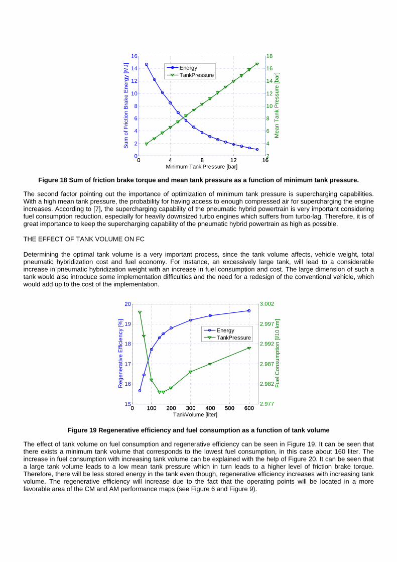
Figure 18 Sum of friction brake torque and mean tank pressure as a function of minimum tank pressure.
The second factor pointing out the importance of optimization of minimum tank pressure is supercharging capabilities. With a high mean tank pressure, the probability for having access to enough compressed air for supercharging the engine increases. According to [7], the supercharging capability of the pneumatic hybrid powertrain is very important considering fuel consumption reduction, especially for heavily downsized turbo engines which suffers from turbo-lag. Therefore, it is of great importance to keep the supercharging capability of the pneumatic hybrid powertrain as high as possible.
THE EFFECT OF TANK VOLUME ON FC
Determining the optimal tank volume is a very important process, since the tank volume affects, vehicle weight, total pneumatic hybridization cost and fuel economy. For instance, an excessively large tank, will lead to a considerable increase in pneumatic hybridization weight with an increase in fuel consumption and cost. The large dimension of such a tank would also introduce some implementation difficulties and the need for a redesign of the conventional vehicle, which would add up to the cost of the implementation.
Figure 19 Regenerative efficiency and fuel consumption as a function of tank volume
The effect of tank volume on fuel consumption and regenerative efficiency can be seen in Figure 19. It can be seen that there exists a minimum tank volume that corresponds to the lowest fuel consumption, in this case about 160 liter. The increase in fuel consumption with increasing tank volume can be explained with the help of Figure 20. It can be seen that a large tank volume leads to a low mean tank pressure which in turn leads to a higher level of friction brake torque. Therefore, there will be less stored energy in the tank even though, regenerative efficiency increases with increasing tank volume. The regenerative efficiency will increase due to the fact that the operating points will be located in a more favorable area of the CM and AM performance maps (see Figure 6 and Figure 9).
0 4 8 12 160
2
4
6
8
10
12
14
16
Su
m o
f Fric
tion
Bra
ke E
ne
rgy
[MJ]
Minimum Tank Pressure [bar]
0 4 8 12 162
4
6
8
10
12
14
16
18
Me
an
Ta
nk
Pre
ssu
re [b
ar]
EnergyTankPressure
0 100 200 300 400 500 60015
16
17
18
19
20
Re
ge
ne
rativ
e E
ffici
en
cy [%
]
TankVolume [liter]
0 100 200 300 400 500 6002.977
2.982
2.987
2.992
2.997
3.002
Fu
el C
on
sum
ptio
n [l
/10
km
]
EnergyTankPressure
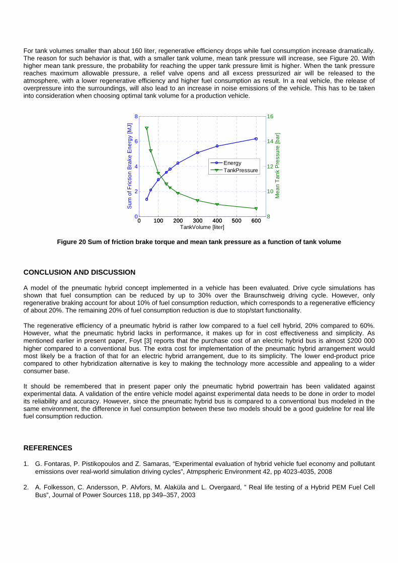
For tank volumes smaller than about 160 liter, regenerative efficiency drops while fuel consumption increase dramatically. The reason for such behavior is that, with a smaller tank volume, mean tank pressure will increase, see Figure 20. With higher mean tank pressure, the probability for reaching the upper tank pressure limit is higher. When the tank pressure reaches maximum allowable pressure, a relief valve opens and all excess pressurized air will be released to the atmosphere, with a lower regenerative efficiency and higher fuel consumption as result. In a real vehicle, the release of overpressure into the surroundings, will also lead to an increase in noise emissions of the vehicle. This has to be taken into consideration when choosing optimal tank volume for a production vehicle.
Figure 20 Sum of friction brake torque and mean tank pressure as a function of tank volume
CONCLUSION AND DISCUSSION
A model of the pneumatic hybrid concept implemented in a vehicle has been evaluated. Drive cycle simulations has shown that fuel consumption can be reduced by up to 30% over the Braunschweig driving cycle. However, only regenerative braking account for about 10% of fuel consumption reduction, which corresponds to a regenerative efficiency of about 20%. The remaining 20% of fuel consumption reduction is due to stop/start functionality.
The regenerative efficiency of a pneumatic hybrid is rather low compared to a fuel cell hybrid, 20% compared to 60%. However, what the pneumatic hybrid lacks in performance, it makes up for in cost effectiveness and simplicity. As mentioned earlier in present paper, Foyt [3] reports that the purchase cost of an electric hybrid bus is almost $200 000 higher compared to a conventional bus. The extra cost for implementation of the pneumatic hybrid arrangement would most likely be a fraction of that for an electric hybrid arrangement, due to its simplicity. The lower end-product price compared to other hybridization alternative is key to making the technology more accessible and appealing to a wider consumer base.
It should be remembered that in present paper only the pneumatic hybrid powertrain has been validated against experimental data. A validation of the entire vehicle model against experimental data needs to be done in order to model its reliability and accuracy. However, since the pneumatic hybrid bus is compared to a conventional bus modeled in the same environment, the difference in fuel consumption between these two models should be a good guideline for real life fuel consumption reduction.
REFERENCES
1. G. Fontaras, P. Pistikopoulos and Z. Samaras, “Experimental evaluation of hybrid vehicle fuel economy and pollutant emissions over real-world simulation driving cycles”, Atmpspheric Environment 42, pp 4023-4035, 2008
2. A. Folkesson, C. Andersson, P. Alvfors, M. Alaküla and L. Overgaard, ” Real life testing of a Hybrid PEM Fuel Cell Bus”, Journal of Power Sources 118, pp 349–357, 2003
0 100 200 300 400 500 6000
2
4
6
8
Su
m o
f Fric
tion
Bra
ke E
ne
rgy
[MJ]
TankVolume [liter]
0 100 200 300 400 500 6008
10
12
14
16
Me
an
Ta
nk
Pre
ssu
re [b
ar]
EnergyTankPressure

3. G. Foyt, “Demonstration and Evaluation of Hybrid Diesel-Electric Transit Buses – Final Report”, Connecticut Academy of Science and Engineering R, CT-170-1884-F-05-10, 2005
4. M. Schechter, “Regenerative Compression Braking – a Low Cost Alternative to Electric Hybrids”, SAE Paper 2000-01-1025, 2000
5. C. Tai, T-C Tsao, M. Levin, G. Barta and M. Schechter, “Using Camless Valvetrain for Air Hybrid Optimization”, SAE Paper 2003-01-0038, 2003
6. I. Vasile, P. Higelin, A. Charlet and Y. Chamaillard, “Downsized engine torque lag compensation by pneumatic hybridization, 13th International Conference on Fluid Flow Technologies, 2006
7. C. Dönitz, I. Vasile, C. Onder and L. Guzzella, “ Realizing a Concept for High Efficiency and Excellent Drivability: The Downsized and Supercharged Hybrid Pneumatic Engine”, SAE paper 2009-01-1326, 2009
8. S. Trajkovic, P. Tunestål and B. Johansson, “Simulation of a Pneumatic Hybrid Powertrain with VVT in GT-Power and Comparison with Experimental Data”, SAE paper 2009-01-1323, 2009
9. M. Andersson, B. Johansson and A. Hultqvist, “An Air Hybrid for High Power Absorption and Discharge”, SAE paper 2005-01-2137, 2005
10. P.K. Chiang, “Two-Mode Urban Transit Hybrid Bus In-Use Fuel Economy Results from 20 Million Fleet Miles”, SAE paper 2007-01-0272, 2007
11. N-O. Nylund, K. Erkkilä and T. Hartikka, “Fuel consumption and exhaust emissions of urban buses”, VTT Research Notes 2373, 2007
12. N-O. Nylund, K. Erkkilä, N. Clark and G. Rideout, “Evaluation of duty cycles for heavyduty urban vehicles”, VTT Research Notes 2396, 2007
13. S. Trajkovic, P. Tunestål and B. Johansson, “Introductory Study of Variable Valve Actuation for Pneumatic Hybridization”, SAE Paper 2007-01-0288, 2007
14. S. Trajkovic, P. Tunestål and B. Johansson, “Investigation of Different Valve Geometries and Valve Timing Strategies and their Effect on Regenerative Efficiency for a Pneumatic Hybrid with Variable Valve Actuation”, SAE Paper 2008-01-1715, 2008
15. M. Alaküla, K. Jonasson, C. Andersson, B. Simonsson, S. Marksell, “Hybrid Drive Systems for Vehicles - Part 1”, Department of Industrial Electrical Engineering and Automation, Lund University, 2004. Available at: http://www.lu.se/o.o.i.s?id=12683& postid=588012, Last accessed 16 October 2009.
16. K. Svensson, “Variable Compression Ratio for increasing the Power Density of Heavyduty Diesel Engines”, Master Thesis, Lund Institute of Technology, Lund, Sweden, 2004.
17. C. Andersson, “On auxiliary systems in commercial vehicles”, Ph.D. Thesis, Department of Industrial Electrical Engineering and Automation, Lund Institute of Technology, Lund, Sweden, 2004

CONTACT
Sasa Trajkovic, PhD student, Msc M. E.
E-mail: [email protected]
Phone: +46-763-161804
DEFINITIONS, ACRONYMS, ABBREVIATIONS
AM: Air-motor Mode
APAM: Air-Power Assist Mode
BDC: Bottom dead Centre
CM: Compressor Mode
DI: Direct Injection
FC: Fuel Consumption
ICE: Internal Combustion Engine
IMEP: Indicated Mean Effective Pressure
PEM: Proton Exchange Membrane
RB: Regenerativ Braking
SI: Spark Ignition
SSM: Stop-Start Mode
S/S: Stop/Start Functionality
TDC: Top Dead Centre

APPENDIX A
The maximum IMEP that can be achieved at a certain tank pressure can be seen in Figure 21 where a PV-diagram shows how an ideal cycle regarding maximum engine load looks like. At BDC the tank valve opens and the cylinder is charged so that the pressure in the cylinder equals the tank pressure. As the piston travels away from BDC, the cylinder pressure will remain constant assuming that the tank is of infinite volume. At TDC the tank valve closes while inlet valve opens and a blowdown of compressed air through the inlet port occurs. As the piston travels away from TDC air enters the cylinder through the inlet port and keeps the volume in the cylinder constant. This entire process is ideal, and cannot be achieved in reality, but shows the absolute maximum achievable engine load at a certain tank pressure.
Figure 21 PV-diagram of maximum achievable engine load during on engine cycle of CM operation
The equation for calculating the maximum theoretical IMEP at a certain tank pressure level is quiet simple:
(1)
where pim = inlet manifold pressure
Here is how it is derived:
The conventional way of calculating IMEP is:
∮ (2)
where Vd = displacement volume of the engine
p = pressure inside the cylinder
dV = is the change in volume
Since the pressure is constant between points 1-2 and 3-4, equation 2 can now be written as:
∗ (3)
The pressure in point 2 is equal to the tank pressure and the pressure in point 3 is equal to the inlet manifold pressure. This leads to the following equation:
This is the same as equation 1.
The same line of argument can be applied for AM just in opposite direction (4-1) with the same outcome, as a result. However, during AM it is not wise to achieve maximum achievable engine load since the entire charge of compressed air will be lost when the inlet valve opens at BDC with a extremely low efficiency as a result.

Paper 5

1 Copyright © 2010 by ASME
Proceedings of the ASME 2010 Internal Combustion Engine Division Fall Technical Conference ICEF2010
September 12-15, 2010, San Antonio, Texas, USA
ICEF2010-35093
A SIMULATION STUDY QUANTIFYING THE EFFECTS OF DRIVE CYCLE CHARACTERISTICS ON THE PERFORMANCE OF A PNEUMATIC HYBRID BUS
Sasa Trajkovic, Per Tunestål and Bengt Johansson
Division of Combustion Engines, Lund University Lund, Skåne, Sweden
E-mail: [email protected]
ABSTRACT In the study presented in this paper, the effect of different
vehicle driving cycles on the pneumatic hybrid has been investigated. The pneumatic hybrid powertrain has been modeled in GT-Power and validated against experimental data. The GT-Power engine model has been linked with a MATLAB/simulink vehicle model. The engine in question is a single-cylinder Scania D12 diesel engine, which has been converted to work as a pneumatic hybrid. The base engine model, provided by Scania, is made in GT-power and it is based on the same engine configuration as the one used in real engine testing.
Earlier studies have shown a great reduction in fuel consumption with the pneumatic hybrid compared to conventional vehicles of today. However, most of these studies have been completely of theoretical nature. In this paper, the engine model is based on and verified against experimental data, and therefore more realistic results can be expected.
The intent with the vehicle driving cycle simulation is to investigate the potential of a pneumatic hybrid bus regarding reduction in fuel consumption (FC) compared to a traditional internal combustion engine (ICE) powered bus.
The results show that the improvement in fuel economy due to pneumatic hybridization varies heavily with choice of drive cycle. The New York bus drive cycle shows a reduction of up to 58 % for the pneumatic hybrid while the FIGE drive cycle only shows a reduction of 8%. What all cycles have in common is that the main part of the fuel consumption reduction comes from the start/stop-functionality, while regenerative braking only account for a modest part of up to about 12% of the fuel consumption. The results also show that the optimal pressure tank volume varies with drive cycles, ranging from 60 to over 500 liters.
INTRODUCTION Growing environmental concerns, together with higher
fuel prices, has created a need for cleaner and more efficient
alternatives to the propulsion systems of today. Currently, the majority of all vehicles are equipped with combustion engines having a maximum thermal efficiency of 30-40%. The average efficiency is much lower, especially during city driving since it involves frequent starts and stops.
The most popular solution to meet the demand for better fuel economy today is the electric hybrid. Almost every car manufacturer is working on an electric hybrid prototype and a few already have a product on the market. Electric hybrids offer impressive reductions in FC. According to Fontaras et al. [1], electric hybrids offer up to 60% lower FC compared to conventional gasoline vehicles. Folkesson et al. [2] have shown a reduction of over 40% in FC for a hybrid PEM fuel cell bus compared to a conventional bus.
The main drawbacks with electric hybrids are that they require an additional propulsion system and large heavy batteries with a limited life-cycle. This introduces extra manufacturing costs which are compensated by a higher end-product price. For instance, the purchase cost for a new electric hybrid bus is almost $200 000 higher compared to a conventional bus [3].
One way of keeping the extra hybridization cost as low as possible compared to a conventional vehicle, is the introduction of the pneumatic hybrid. It does not require an expensive extra propulsion source and it works in a way similar to the electric hybrid. During deceleration of the vehicle, the engine is used as a compressor that converts the kinetic energy contained in the vehicle into energy in the form of compressed air which is stored in a pressure tank. After a standstill the engine is used as an air-motor that utilizes the pressurized air from the tank in order to accelerate the vehicle. The system supports stop/start functionality, which means that the engine can be shut off during a full stop and thus eliminating idle losses [4,5]. The pneumatic hybrid also offers elimination of the “turbo-lag” in turbocharged engines by supercharging the engine with pressurized air [6,7].

2 Copyright © 2010 by ASME
In the study presented in this paper the focus has been on fuel consumption and pneumatic hybrid performance over 10 different driving cycles. For this purpose, a simulink model of a pneumatic hybrid bus has been developed. The model is supplemented with pneumatic hybrid powertrain performance maps from an experimentally validated GT-power engine model [8].
THE PNEUMATIC HYBRID POWERTRAIN Pneumatic hybridization brings new modes of operation in
addition to the conventional ICE operation. The main pneumatic hybrid modes of operation are the air-motor mode (AM) and compressor mode (CM) in which the ICE is used as a compressor and expander, respectively. Another possible mode of operation is the air-power assist mode (APAM) during which the compressed air is used for supercharging the engine in order to meet higher torque demand. As the electric hybrid, the pneumatic hybrid powertrain allows the ICE to be shut off during a standstill and when the gas pedal is released. In this way, idle can be eliminated with a reduction in fuel consumption and exhaust emissions as a result. This mode is referred to as stop/start mode (SSM).
The various modes of operation have been thoroughly described in earlier publications by the author [8,9,10]. Therefore, only a short summary of the main modes of operation will be given here.
Compressor Mode The compressor mode is activated instead of the friction
brakes during vehicle deceleration. During compressor mode the engine is used as a 2-stroke compressor which converts the kinetic energy of the vehicle into potential energy in the form of compressed air.
The compressor mode starts with an intake stroke. The inlet valve opens at top dead centre (TDC) or shortly after and brings fresh air to the cylinder, and closes around bottom dead centre (BDC). During the following stoke, as the piston moves away from BDC, the charge of fresh air is compressed until the tank valve opens. The tank valve is connected to a pressure tank in which the compressed air is stored. A simple illustration of compressor mode can be seen in Figure 1.
For maximum braking power, the tank valve should open in the vicinity of BDC during the compressor stroke. In this way, a specific brake torque of over 300 Nm per liter engine displacement can be achieved, as will be shown later on in this paper.
Air-motor Mode The air-motor mode is activated during the subsequent
acceleration after a standstill. During air-motor mode the engine is used as a 2-stoke air-motor/expander, converting the compressed air into kinetic energy.
The air-motor mode starts with an expansion stroke. At TDC, the tank valve opens and compressed air fills the cylinder. The closing of the valve occurs somewhere between TDC and BDC, depending on the torque demand. At BDC, the
inlet valve opens and remains open during the compression stroke. The air-motor mode is illustrated in Figure 2.
Figure 1 Illustration of Compressor Mode. I) Intake of fresh
air, II) Compression of air and pressure tank charging. Right port is connected to the pressure tank.
Figure 2 Illustration of Air-Motor Mode. I) Intake of
compressed air, II) Air venting. Right port is connected to the pressure tank.
The required amount of admitted charge into the cylinder
depends on the current power demand, and is controlled by the closing point of the tank valve. For maximum AM efficiency the tank valve should close in such a way that when the piston reaches BDC, the cylinder pressure reaches atmospheric conditions. Late closing of the tank valve will lead to higher power but a low AM efficiency since the cylinder pressure at BDC will be above atmospheric conditions, with a blow down through the intake port when the inlet valve opens as a result.
VEHICLE MODELING The base vehicle model is made in MATLAB/Simulink and
is based upon a typical vehicle for personal transport and weighs 1300 kg. It is modeled with a 1.5 liter diesel engine based on maps obtained experimentally. The model has been developed by the Department of Industrial Electrical

3 Copyright © 2010 by ASME
Engineering and Automation (IEA) at Lund University and has been thoroughly described in [11].
Since the purpose of the study presented in this paper was to evaluate the pneumatic hybrid powertrain implemented in a city bus, the model needed to be modified. Below, a list of the most significant modifications is presented.
The original ICE model was based on a 1.5L spark
ignited (SI) 4-cylinder engine, while the city bus engine was based on a 12L direct injected (DI) 6-cylinder engine. Therefore, the original ICE model was replaced by an ICE model based on data from a GT-Power model of a SCANIA D12 engine model designed by SCANIA and validated by Svensson [12]. Geometric properties of the engine can be seen in Table 1.
All electric-hybrid related components were removed
and replaced by pneumatic hybrid components. The pneumatic hybrid powertrain performance maps are generated in a GT-Power model validated against experimental data [8].
Vehicle specific data like weight, frontal area,
maximum torque and power, were updated with suitable data for the chosen vehicle. The most significant vehicle data can be seen in Table 2. The auxiliary power demand of 4 kW is a mean value for the entire Braunschweig drive cycle and has been chosen in accordance with [13].
Figure 3 and Figure 4 show the top level of the pneumatic
hybrid bus model and the pneumatic hybrid subsystem, respectively.
Drive Cycles In [14], the pneumatic hybrid performance over the
Braunschweig drive cycle was investigated with promising results. However, it is of great importance to study how performance will change with a change in driving pattern. In this way, the effect of parameters such as acceleration, average speed and stops/km on fuel consumption can be examined. Therefore, in the present study, 10 different drive cycles were investigated. Some basic parameters of all the chosen drive cycles can be seen in Table 3. Figure 5 and Figure 6 illustrates the vehicle speed as a function of time for two drive cycles, the New York bus cycle and the FIGE (Forschungsinstitut Gerausche und Erschutterungen) drive cycle. The New York bus cycle is characterized by a low maximum and average speed together with a high rate of stops/km. The FIGE drive cycle consists of three parts, including city, rural and motorway driving where the duration of each part is 600s.
Figure 7 and Figure 8 show the mean and maximum acceleration/deceleration, respectively, for all drive cycles.
They illustrate the rate of aggressiveness of the different drive cycles. For instance, the CBD drive cycle has the highest mean acceleration and deceleration which together with a relatively
Table 1 Geometric properties of the SCANIA D12 diesel engine
Displaced Volume/Cylinder 1966 cm3
Bore 127.5 mm
Stroke 154 mm
Connecting Rod Length 255 mm Number of Valves 4 Compression Ratio 18:1 Piston type Bowl Inlet valve diameter 45 mm
Exhaust valve diameter 41 mm
Valve Timing Variable
Table 2 Vehicle data for the simulated city bus
Total Vehicle Weight 15000 kg
Wheel Radius, rw 0.517 m
Air Resistance, Cd 0.75
Rolling Resistance, Cr 0.008
Frontal Area 7.5 m2
Auxiliary power demand 4 kW
Maximum Vehicle Speed 80 km/h
Pressure Tank Volume 40 liter
Starting tank pressure 23.7 bar
Lower tank pressure limit 8 bar
Upper tank pressure limit 27 bar high maximum acceleration and deceleration, makes this drive cycle quite aggressive. The New York and Manhattan bus drive cycles both have very low mean and maximum acceleration/deceleration which makes them the least aggressive of all chosen drive cycles. The effect of the aggressiveness on pneumatic hybrid performance will be discussed later on in the paper.
Figure 9 illustrates mean and maximum speed during the chosen drive cycles. The bus cycles shows a quite low mean speed which can be explained by the high ratio of stops/km compared to the non-bus cycles .The FIGE drive cycle show the highest mean speed of all drive cycles, mainly due to the fact that this drive cycle contains a motorway-driving section.
SIMULATION RESULTS The content of this section can be divided into three parts.
In the first part, the pneumatic hybrid powertrain performance maps generated in GT-Power are discussed. The second part of this section deals with the results obtained from the vehicle simulation. Finally, in the third part, different parameters affecting the tank volume for different drive cycles are investigated.

4 Copyright © 2010 by ASME
Figure 3 Top level of the pneumatic hybrid bus model
Figure 4 The Pneumatic hybrid specific subsystem
Table 3 Basic parameters of the different drive cycles used in present study ( CBD=Central Business District, OC=Orange
County, CSC=City Suburban Cycle, HD-UDDS= Heavy-Duty Urban Dynamometer Driving Schedule)
Cycle Braunschweig
Bus CBD NewYork
Bus NewYork Composite
Manhattan Bus
OC Bus
FIGE CSC Japan JE05
HD-UDDS
Time [s] 1740 560 600 1029 1089 1909 1800 1700 1829 1060 Distance
[km] 10.87 3.29 0.99 4.03 3.32 10.53 29.49 10.75 13.89 8.94
Avg. Speed [km/h]
22.50 21.13 5.94 14.11 10.99 19.85 58.98 22.77 27.33 30.32
Max Speed [km/h]
58.20 32.19 49.57 57.94 40.88 65.39 91.10 70.56 87.60 93.34
Idle [%] 25.34 17.65 65.52 33.14 35.98 21.27 0.00 23.29 25.19 33.27 Max Acc. [m/s^2]
2.42 0.89 0.31 2.07 0.22 1.82 3.83 1.14 1.59 1.96
Max Decl. [m/s^2]
3.58 2.24 0.22 1.96 0.27 2.29 4.03 1.77 1.83 2.07
Stops 30 14 12 21 21 32 0 14 15 15
Stops/km 2.76 4.25 12.13 5.21 6.32 3.04 0.00 1.30 1.08 1.68

5 Copyright © 2010 by ASME
Figure 5 Vehicle speed during the New York Bus drive cycle
Figure 6 Vehicle speed during the FIGE drive cycle
Figure 7 Mean acceleration and deceleration during the
different drive cycles
Figure 8 Maximum acceleration and deceleration during
different drive cycles
Figure 9 Mean and maximum speed during different drive cycles
Pneumatic Hybrid Powertrain Performance Maps In [8], a model of the pneumatic hybrid powertrain based
on the SCANIA D12 engine used in this paper was developed in GT-Power and validated against experimental data. In the study presented in this paper, the same model has been used in order to create performance maps of both AM and CM. The performance maps shows the mass flow of air into or out from the tank (depending on the mode of operation) as a function of engine load and tank pressure. Figure 10 and Figure 11 show the performance map of CM while Figure 13 and Figure 14 show the performance map of AM. All performance maps shown are for one cylinder only.
From Figure 10 and Figure 11, it can be seen that, during CM operation, the engine torque and IMEP can reach very high levels. According to Appendix A, the maximum achievable theoretical IMEP can be calculated with following simple equation:
(1)
0 100 200 300 400 500 6000
10
20
30
40
50
Time [s]
Ve
hic
le S
pe
ed
[km
/h]
0 500 1000 15000
20
40
60
80
100
Time [s]
Ve
hic
le S
pe
ed
[km
/h]
-2
-1
0
1
2
Acc
eler
atio
n [
m/s
2]
CBD
NYbus
NYcom
p
Man
h
OCbus
BraunS
FIGE
CSCJE
05
UDDS
Mean AccelerationMean Deceleration
-6
-4
-2
0
2
4
6
Acc
eler
atio
n [
m/s
2]
CBD
NYbus
NYcom
p
Man
h
OCbus
BraunS
FIGE
CSCJE
05
UDDS
Max AccelerationMax Deceleration
0
20
40
60
80
100
Sp
eed
[km
/h]
CBD
NYbus
NYcom
p
Man
h
OCbus
BraunS
FIGE
CSCJE
05
UDDS
Mean SpeedMax Speed
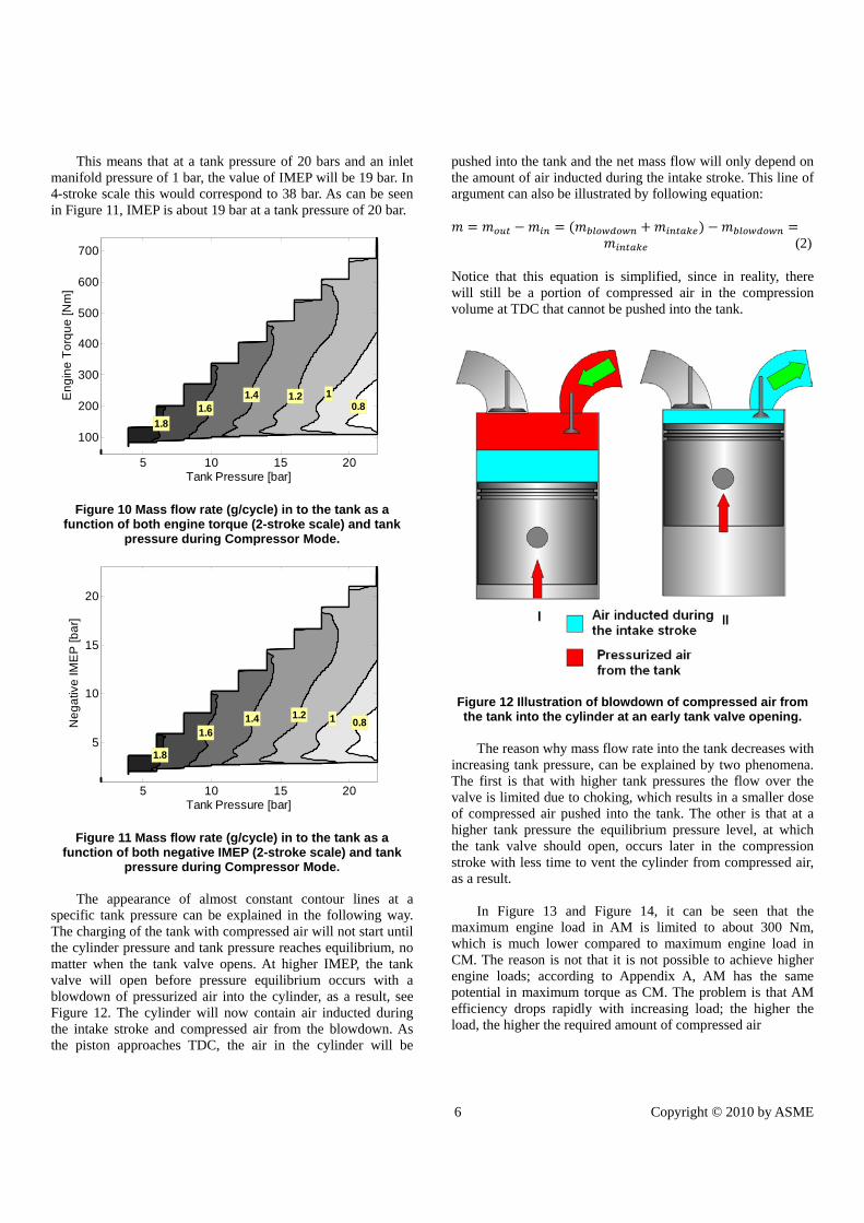
6 Copyright © 2010 by ASME
This means that at a tank pressure of 20 bars and an inlet manifold pressure of 1 bar, the value of IMEP will be 19 bar. In 4-stroke scale this would correspond to 38 bar. As can be seen in Figure 11, IMEP is about 19 bar at a tank pressure of 20 bar.
Figure 10 Mass flow rate (g/cycle) in to the tank as a function of both engine torque (2-stroke scale) and tank
pressure during Compressor Mode.
Figure 11 Mass flow rate (g/cycle) in to the tank as a function of both negative IMEP (2-stroke scale) and tank
pressure during Compressor Mode. The appearance of almost constant contour lines at a
specific tank pressure can be explained in the following way. The charging of the tank with compressed air will not start until the cylinder pressure and tank pressure reaches equilibrium, no matter when the tank valve opens. At higher IMEP, the tank valve will open before pressure equilibrium occurs with a blowdown of pressurized air into the cylinder, as a result, see Figure 12. The cylinder will now contain air inducted during the intake stroke and compressed air from the blowdown. As the piston approaches TDC, the air in the cylinder will be
pushed into the tank and the net mass flow will only depend on the amount of air inducted during the intake stroke. This line of argument can also be illustrated by following equation:
(2)
Notice that this equation is simplified, since in reality, there will still be a portion of compressed air in the compression volume at TDC that cannot be pushed into the tank.
Figure 12 Illustration of blowdown of compressed air from the tank into the cylinder at an early tank valve opening.
The reason why mass flow rate into the tank decreases with
increasing tank pressure, can be explained by two phenomena. The first is that with higher tank pressures the flow over the valve is limited due to choking, which results in a smaller dose of compressed air pushed into the tank. The other is that at a higher tank pressure the equilibrium pressure level, at which the tank valve should open, occurs later in the compression stroke with less time to vent the cylinder from compressed air, as a result.
In Figure 13 and Figure 14, it can be seen that the
maximum engine load in AM is limited to about 300 Nm, which is much lower compared to maximum engine load in CM. The reason is not that it is not possible to achieve higher engine loads; according to Appendix A, AM has the same potential in maximum torque as CM. The problem is that AM efficiency drops rapidly with increasing load; the higher the load, the higher the required amount of compressed air
Tank Pressure [bar]
En
gin
e T
orq
ue
[Nm
]
1.8
1.61.4 1.2 1
0.8
5 10 15 20
100
200
300
400
500
600
700
Tank Pressure [bar]
Ne
ga
tive
IME
P [b
ar]
1.8
1.61.4 1.2 1 0.8
5 10 15 20
5
10
15
20

7 Copyright © 2010 by ASME
Figure 13 Mass flow rate (g/cycle) out from the tank as a function of both engine torque and tank pressure during
Air-Motor Mode.
Figure 14 Mass flow rate (g/cycle) out from the tank as a function of both positive IMEP and tank pressure during
Air-Motor Mode.
becomes. This in turn means that the tank valve closing will occur much later in the cycle compared to optimal closing. This results in that the cylinder pressure level at the time of inlet valve opening (around BDC), will be higher compared to the inlet manifold pressure. Therefore, there will be a blowdown of compressed air into the intake manifold, without any positive work being extracted from it, with a decrease in AM efficiency, as a result. This behavior is confirmed by Figure 15, where a PV-diagram of one cycle during AM can be seen. The illustrated operating point corresponds to the upper right corner of Figure 13 and Figure 14. At inlet valve opening (point 3), the cylinder pressure is about 6 bar and reaches almost 1 bar at inlet valve closing (point 4). This is a pressure loss of about 5
Figure 15 PV-diagram of one cycle during Air-Motor Mode illustrating the blowdown of compressed air through the
inlet port at high engine loads. bar, which corresponds to an energy loss of approximately 1 kJ per cycle.
Drive Cycle Simulation Results Figure 16 and Figure 17 show how tank pressure varies
during the New York bus cycle and FIGE drive cycle, respectively. The New York cycle is characterized by a high rate of stops/km and frequent idling, which in Figure 16 is illustrated by constant pressure after a prece ding increase in tank pressure. The FIGE drive cycle consists of three parts, including city, rural and motorway driving. The city driving part of the FIGE cycle shows similar patterns of frequent change in tank pressure as seen during the New York cycle. During the rural driving section, the change in tank pressure becomes less frequent and during the last part, motorway driving, there is almost no charging of the pressure tank. During motorway driving, the vehicle is propelled at almost constant speed with almost no braking and thus no compressed air will be generated. Another thing that can be seen in Figure 16 and Figure 17, is that the minimum tank pressure is limited to 8 bar. The minimum tank pressure has been chosen in accordance with [14] and 8 bar is the lower pressure limit at which minimum FC can be observed.
From Figure 16 and Figure 17 it can also be noticed that the initial tank pressure has been set to the same level as at the end of the driving cycle. In this way, the influence of starting tank pressure on pneumatic hybrid performance was eliminated. If, for instance, the initial tank pressure would have been set to a pressure lower than the pressure at the end of the cycle, the pneumatic hybrid efficiency would have been affected negatively, due to the fact that the last portion of captured and stored braking energy would never have been used.
Tank Pressure [bar]
En
gin
e T
orq
ue
[Nm
]
2
4
6
8
10
5 10 15 20
50
100
150
200
250
Tank Pressure [bar]
Po
sitiv
e IM
EP
[ba
r]
2
4
6
8
10
5 10 15 20
1
2
3
4
5
6
7
8
9
0 0.5 1 1.5 2 2.50
5
10
15
20
25
Cylinder Volume [liter]
Cyl
ind
er
Pre
ssu
re [b
ar]
Torque = 250 NmIMEP = 8.5 barTankPressure = 17.4 bar
4
3
21
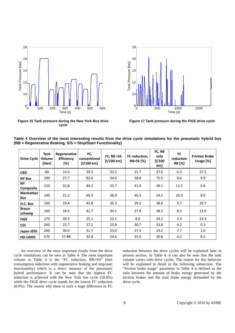
8 Copyright © 2010 by ASME
Figure 16 Tank pressure during the New York Bus drive cycle
Figure 17 Tank pressure during the FIGE drive cycle
Table 4 Overview of the most interesting results from the drive cycle simulations for the pneumatic hybrid bus (RB = Regenerative Braking, S/S = Stop/Start Functionality)
Drive Cycle Tank
Volume [liter]
Regenerative Efficiency
[%]
FC, conventional [l/100 km]
FC, RB +SS [l/100 km]
FC reduction, RB+SS [%]
FC, RB only [l/100 km]
FC reduction RB [%]
Friction Brake Usage [%]
CBD 60 14.3 39.5 33.3 15.7 37.0 6.3 27.5
NY Bus 100 27.7 82.6 34.0 58.8 75.5 8.6 4.9
NY Composite
110 32.8 44.2 25.7 41.9 39.1 11.5 0.9
Manhattan Bus
140 21.3 60.3 36.0 40.3 54.1 10.3 8.0
O.C. Bus 150 19.4 42.8 30.3 29.2 38.6 9.7 10.7
Braun‐schweig
160 18.5 41.7 30.1 27.8 38.2 8.5 13.0
FIGE 170 28.3 25.1 23.1 8.0 24.2 3.4 22.4
CSC 260 22.7 37.2 25.8 30.7 33.8 9.2 0.3
Japan JE05 260 30.0 31.7 23.0 27.4 29.2 7.7 1.0
HD‐UDDS 570 27.88 32.8 24.6 25.0 30.8 6.2 8.3
An overview of the most important results from the drive cycle simulations can be seen in Table 4. The most important column in Table 4 is the “FC reduction, RB+SS” (fuel consumption reduction with regenerative braking and stop/start functionality) which is a direct measure of the pneumatic hybrid performance. It can be seen that the highest FC reduction is achieved with the New York bus cycle (58.8%) while the FIGE drive cycle stands for the lowest FC reduction (8.0%). The reason why there is such a huge difference in FC
reduction between the drive cycles will be explained later in present section. In Table 4, it can also be seen that the tank volume varies with drive cycles. The reason for this behavior will be explained in detail in the following subsection. The “friction brake usage” parameter in Table 4 is defined as the ratio between the amount of brake energy generated by the friction brakes and the total brake energy demanded by the drive cycle.
0 100 200 300 400 500 6008
10
12
14
16
18
Time [s]
Ta
nk
Pre
ssu
re [b
ar]
0 500 1000 15008
10
12
14
16
18
Time [s]
Ta
nk
Pre
ssu
re [b
ar]

9 Copyright © 2010 by ASME
Figure 18 and Figure 19 give a clearer view of the total fuel consumption reduction and fuel consumption reduction only due to regenerative braking, respectively. By comparing the two figures to one another, it can clearly be concluded that the Stop/Start functionality can be accredited for a considerable part of the reduction in fuel consumption, since the contribution from regenerative braking is quite modest. It can also be seen that both these figures show similar trends in FC reduction for the different drive cycles. This is quite logical since the reduction in FC comes from regenerative braking and stop/start functionality. Every stop is accompanied by pneumatic hybrid operation - a segment of regenerative braking before the stop and a segment of air-motor operation after the stop. This means that the ratio of stops to pneumatic hybrid operation is about 1 which explains the behavior of similar trends observed in Figure 18 and Figure 19. However, this explanation is not entirely correct, since a stop followed by a long idle period would lead to a much larger reduction in FC compared to what the accompanying pneumatic hybrid operation could achieve. This is the case with the New York bus cycle which shows the largest discrepancy from this explanation. The reason is that the New York bus cycle has the highest rate of idle (65.5%) of all drive cycles examined and therefore a larger part of the FC reduction will come from the elimination of the idle period.
Figure 18 Fuel consumption reduction for the different
drive cycles
Figure 20 illustrates how fuel consumption reduction is related to the frequency of stopping in the various cycles. As can be seen, the data have been fitted to a linear regression and the correlation is quite strong. This can be explained by the fact that each stop is accompanied by pneumatic hybrid operation and an idle period, both contributing to a reduction in FC. This means that a drive cycle involving frequent stops has the highest potential in FC reduction. The New York bus cycle shows, in accordance with Figure 20, the highest FC reduction and has the highest rate of stops per kilometer, while the FIGE drive cycle, which is predominantly a high-speed cycle and involves very few stops, has the lowest FC reduction of all drive cycles examined.
Figure 19 Fuel consumption reduction achieved only with regenerative braking for the different drive cycles (RB =
Regenerative Braking)
Figure 20 Fuel consumption reduction for all drive cycles
as a function of stops/km
Figure 21 Fuel consumption reduction as a function of idle
0
10
20
30
40
50
60
Fu
el C
on
su
mp
tio
n R
edu
ctio
n [
%]
CBD
NYbus
NYcom
p
Man
h
OCbus
BraunS
FIGE
CSCJE
05
UDDS
0
2
4
6
8
10
12
14
Fu
el C
on
sum
pti
on
Red
uct
ion
RB
on
ly [
%]
CBD
NYbus
NYcom
p
Man
h
OCbus
BraunS
FIGE
CSCJE
05
UDDS
0 2 4 6 8 10 12 140
10
20
30
40
50
60
70
Stops/Km
Fu
el C
on
sum
ptio
n R
ed
uct
ion
[%]
MeasurmentLinear fit
R2=0.7603
0 20 40 60 800
10
20
30
40
50
60
70
Idle [%]
Fu
el C
on
sum
ptio
n R
ed
uct
ion
[%]
MeasurmentLinear fit
R2=0.7859

10 Copyright © 2010 by ASME
The relation between fuel consumption reduction and idle duration can be seen in Figure 21. It is not surprising to see that the reduction of fuel consumption will increase with the rate of idle. With the pneumatic hybrid powertrain, the engine can be completely shut-off during a stand-still, thus eliminating idle and no fuel will be used during this period. The longer this period is the more FC is reduced. The results in Figure 20 and Figure 21 are closely related since a complete stop is most likely followed by a period of idle and there is a synergy between the two affecting the FC positively. A cycle with long periods of idle but few stops will see lower beneficial impacts on FC.
Figure 22 Fuel consumption reduction as a function of
average speed
Figure 23 Stops/km as a function of average speed Figure 22 shows how fuel consumption reduction varies
with average speed. It can be seen that an increase in average speed results in a decrease in fuel consumption reduction. This behavior can be explained with the help of Figure 23, where it can be observed that the average speed decreases with stops/km. A drive cycle with frequent stops, consequently also
contains frequent parts where the vehicle slows down. For instance, a drive cycle representing highway-driving, contains very few stops and a quite high vehicle top speed. This will lead to a high average speed since there will be a low number of decelerations present in the drive cycle decreasing the average speed. The FIGE drive cycle, which is predominantly a high-speed cycle and involves very few stops, has the highest average speed, which results in that the FIGE drive cycle shows the lowest fuel consumption reduction of all drive cycles examined. The New York bus cycle and Manhattan bus cycle are both characterized by low average speed and frequent stops, which results in high fuel consumption reductions.
Figure 24 AM usage ratio for different drive cycles The compressor mode only contributes to FC reduction
indirectly through the air-motor mode. If the air, compressed during CM operation, is not used during AM, there will be no reduction in FC since the captured energy from braking will not be converted to useful work. This implies that the utilization of AM relates better to the FC reduction than the utilization of CM. Therefore a parameter that relates the AM usage in form of supplied AM torque to the amount of drive torque demanded during the entire drive cycle has been derived and can be defined as:
(3)
Figure 24 illustrates how AM usage ratio varies with
different drive cycles. There is a great resemblance between Figure 24 and Figure 18, which implies that AM usage ratio and FC reduction are strongly related. This relation is illustrated in Figure 25 where it can clearly be seen that the FC reduction is an almost linear function of the AM usage ratio. A high AM torque contribution leads to a high decrease in FC. The results from Figure 25 are quite logical since a higher AM torque contribution means that the amount of time that the ICE engine has to kick in to satisfy the drive torque demand decreases.
0 10 20 30 400
10
20
30
40
50
60
70
Average speed [km/h]
Fu
el C
on
sum
ptio
n R
ed
uct
ion
[%]
MeasurmentLinear fit
R2=0.7826
0 5 10 150
5
10
15
20
25
30
35
Ave
rag
e s
pe
ed
[km
/h]
Stops/km [-]
MeasurmentLinear fit
R2=0.8275
0
10
20
30
40
50
AM
usa
ge
rati
o [
%]
CBD
NYbus
NYcom
p
Man
h
OCbus
BraunS
FIGE
CSCJE
05
UDDS

11 Copyright © 2010 by ASME
Figure 25 Fuel consumption reduction as a function of AM
usage ratio.
Figure 26 AM usage ratio as a function of average speed.
Figure 26 shows how the AM usage ratio is related to the
average speed of the vehicle. As discussed earlier, the average speed is strongly related to stops/km. A drive cycle with high average speed contains fewer stops/km compared to a drive cycle with lower average speed. A small number of stops/km means that the amount of time the powertrain will spend in air-motor mode during the drive cycle will be small, and the other way around. Further, this means that a drive cycle with a high average speed contains a low number of stops/km and consequently a lower AM usage ratio, as can be seen in Figure 26.
Investigation of Tank Volume Influence on Drive Cycle Performance
As listed in Table 4, the predicted optimal volume differs for the drive cycles. Figure 27 and Figure 28, illustrate how friction brake usage and mean tank pressure are affected by
Figure 27 Friction brake usage and mean tank pressure as
a function of tank volume for the FIGE drive cycle
Figure 28 Friction brake usage and mean tank pressure as
a function of tank volume for the New York Composite drive cycle
tank volume for two different drive cycles, namely the FIGE drive cycle and the New York Composite drive cycle. Friction brake usage is directly related to the amount of time the powertrain will spend in compressor mode during the drive cycle. A low friction brake usage means that the main part of the braking comes from a high CM activity. It can be seen in both figures that mean tank pressure decreases while friction brake usage increases with increasing tank volume. The reason for this behavior is that the energy that can be stored in the tank during the drive cycle is almost constant, independent of tank volume and since energy stored in the tank is a function of volume and pressure, the pressure in the tank will decrease with increasing tank volume. With references to Figure 10, this decrease in mean tank pressure will lead to a decrease in maximum achievable brake torque during CM which in turn will limit the braking torque generated during CM operation and therefore friction brake usage will increase.
0 10 20 30 40 50 600
10
20
30
40
50
60
AM usage ratio [%]
Fu
el C
on
sum
ptio
n R
ed
uct
ion
[%]
MeasurmentLinear fit
R2=0.9337
0 10 20 30 40 50 600
10
20
30
40
50
AM
usa
ge
ra
tio [%
]
Average Speed [km/h]
MeasurmentLinear fit
R2=0.7162
0 100 200 300 400 500 60016
18
20
22
24
26
Fric
tion
Bra
ke U
sag
e [%
]
TankVolume [liter]
0 100 200 300 400 500 6008
8.5
9
9.5
10
10.5
Me
an
Ta
nk
Pre
ssu
re [b
ar]
BrakesTankPress.
0 100 200 300 400 500 6000
0.3
0.6
0.9
1.2
1.5
1.8
2.1
2.4F
rictio
n B
rake
Usa
ge
[%]
TankVolume [liter]
0 100 200 300 400 500 6008
8.5
9
9.5
10
10.5
11
11.5
12
Me
an
Ta
nk
Pre
ssu
re [b
ar]
BrakesTankPress.

12 Copyright © 2010 by ASME
By comparing Figure 27 to Figure 28, it can be seen that the results show similar trends in both figures and from these results no conclusion can be drawn about why the tank volume varies with drive cycles. Instead, the answer can be found with the help of two other parameters, air mass flow out of the pressure tank during AM operation and AM usage ratio. They are plotted in Figure 29 and Figure 30, respectively, against tank volume.
The positive work done during AM operation due to the expansion of compressed air can be defined as:
∮ (4)
where W is the work done during AM operation, P and dV are the pressure and volume, respectively, of the compressed air inducted into the cylinder. If W is to remain constant while P decreases, dV has to increase. Applied to the AM operation, this means that as the tank pressure decreases, the volume of compressed air inducted into the cylinder have to increase while keeping the work done constant. However if, the tank pressure decreases below the level at which the demanded dV reaches a maximum, i.e when dV equals the cylinder volume of the engine, the torque supply will start to decrease. In other words, the cylinder cannot be filled with enough compressed air in order to satisfy the work demanded by the drive cycle. This can clearly be seen in Figure 29. At first, AM air mass flow increases with tank volume according to the discussion above. At a tank volume of about 100 liter the air mass flow reaches a stagnation point after which it starts to decrease and results in that the demanded torque cannot be satisfied anymore. The same argument can be applied to Figure 30 where AM usage ratio is plotted against tank volume. It can be seen that maximum/optimal AM usage ratio is achieved at a tank volume between 150 and 200 liter. If the tank volume decreases compared to the optimal point, the AM usage ratio
Figure 29 AM air mass flow and mean tank pressure as a
function of tank volume for the Manhattan bus cycle
Figure 30 AM usage ratio as a function of tank volume for
the FIGE drive cycle will also decrease. The reason for this behavior is that the tank volume will be so small that there will not be enough air in the tank to satisfy the torque demand throughout the drive cycle and therefore the ICE will kick in more often with a decrease in AM usage ratio as a result. If the tank volume increases compared to the optimal point, the AM usage ratio will decrease. This decrease occurs due to the inability to fill the cylinder with an adequate amount of air at low tank pressures, as discussed above with reference to Figure 29, and the torque demand cannot be satisfied. The volume at which optimal AM usage ratio occurs is drive cycle specific and explains why optimal predicted tank volume varies with different drive cycles.
CONCLUSION AND DISCUSSION A model of the pneumatic hybrid concept implemented in a
bus has been evaluated for 10 different drive cycles. The simulations have shown that fuel consumption varies heavily with drive cycles. The New York bus drive shows a fuel consumption reduction of up to 58% for the pneumatic hybrid while the FIGE drive cycle only shows a modest fuel consumption reduction of about 8%. It has been shown that regenerative braking only account for up to about 12% of this fuel consumption reduction at best. The remaining fuel consumption reduction is mainly due to the stop/start functionality.
The main reason why fuel consumption varies with different drive cycles is their driving patterns. Average fuel consumption highly depends on parameters such as acceleration, average speed and stops/km. The results indicates that city drive cycles that are not aggressive regarding acceleration and deceleration, have a low average speed and a high number of stops benefit from pneumatic hybrid operation. For drive cycles that are predominantly high-speed cycles and involve very few stops, the pneumatic hybrid will have a modest influence on the improvement of fuel economy.
0 100 200 300 400 500 6000.4
0.42
0.44
0.46
0.48
0.5
AM
Air
Ma
ss F
low
[kg
/s]
Tank Volume [liter]
0 100 200 300 400 500 6000.5
0.7
0.9
1.1
1.3
1.5
Me
an
Ta
nk
Pre
ssu
re [b
ar]
Mass FlowTankPress.
0 100 200 300 400 500 6007.2
7.4
7.6
7.8
8
8.2
Tank Volume [liter]
AM
-to
-IC
E to
rqu
e r
atio
[%]

13 Copyright © 2010 by ASME
The results have shown that optimal pressure tank volume varies with drive cycles, ranging from 60 to over 500 liters. The pressure tank volume highly depends on parameters such as air flow output and the amount of time the powertrain spends in air-motor mode.
It should be remembered that in present paper only the pneumatic hybrid powertrain has been validated against experimental data. A validation of the entire vehicle model against experimental data needs to be done in order to model its reliability and accuracy. However, since the pneumatic hybrid bus is compared to a conventional bus modeled in the same environment, the difference in fuel consumption between these two models should be a good guideline for real life fuel consumption reduction.
REFERENCES 1. G. Fontaras, P. Pistikopoulos and Z. Samaras,
“Experimental evaluation of hybrid vehicle fuel economy and pollutant emissions over real-world simulation driving cycles”, Atmpspheric Environment 42, pp 4023-4035, 2008
2. A. Folkesson, C. Andersson, P. Alvfors, M. Alaküla and L. Overgaard, ” Real life testing of a Hybrid PEM Fuel Cell Bus”, Journal of Power Sources 118, pp 349–357, 2003
3. G. Foyt, “Demonstration and Evaluation of Hybrid Diesel-Electric Transit Buses – Final Report”, Connecticut Academy of Science and Engineering R, CT-170-1884-F-05-10, 2005
4. M. Schechter, “Regenerative Compression Braking – a Low Cost Alternative to Electric Hybrids”, SAE Paper 2000-01-1025, 2000
5. C. Tai, T-C Tsao, M. Levin, G. Barta and M. Schechter, “Using Camless Valvetrain for Air Hybrid Optimization”, SAE Paper 2003-01-0038, 2003
6. I. Vasile, P. Higelin, A. Charlet and Y. Chamaillard, “Downsized engine torque lag compensation by pneumatic hybridization, 13th International Conference on Fluid Flow Technologies, 2006
7. C. Dönitz, I. Vasile, C. Onder and L. Guzzella, “ Realizing a Concept for High Efficiency and Excellent Drivability: The Downsized and Supercharged Hybrid Pneumatic Engine”, SAE paper 2009-01-1326, 2009
8. S. Trajkovic, P. Tunestål and B. Johansson, “Simulation of a Pneumatic Hybrid Powertrain with VVT in GT-Power and Comparison with Experimental Data”, SAE paper 2009-01-1323, 2009
9. S. Trajkovic, P. Tunestål and B. Johansson, “Introductory Study of Variable Valve Actuation for Pneumatic Hybridization”, SAE Paper 2007-01-0288, 2007
10. S. Trajkovic, P. Tunestål and B. Johansson, “Investigation of Different Valve Geometries and Valve Timing Strategies and their Effect on Regenerative Efficiency for a Pneumatic Hybrid with Variable Valve Actuation”, SAE Paper 2008-01-1715, 2008
11. M. Alaküla, K. Jonasson, C. Andersson, B. Simonsson, S. Marksell, “Hybrid Drive Systems for Vehicles - Part 1”, Department of Industrial Electrical Engineering and Automation, Lund University, 2004. Available at: http://www.lu.se/o.o.i.s?id=12683& postid=588012, Last accessed 16 October 2009.
12. K. Svensson, “Variable Compression Ratio for increasing the Power Density of Heavyduty Diesel Engines”, Master Thesis, Lund Institute of Technology, Lund, Sweden, 2004.
13. C. Andersson, “On auxiliary systems in commercial vehicles”, Ph.D. Thesis, Department of Industrial Electrical Engineering and Automation, Lund Institute of Technology, Lund, Sweden, 2004
14. S.Trajkovic, P. Tuenstål and B. Johansson, “Vehicle Driving Cycle Simulation of a Pneumatic Hybrid Bus Based on Experimental Engine Measurments”, SAE Paper 2010-01-0825, 2010
NOMENCLATURE AM: Air-motor Mode APAM: Air-Power Assist Mode BDC: Bottom dead Centre CM: Compressor Mode DI: Direct Injection dV: change in Volume FC: Fuel Consumption ICE: Internal Combustion Engine IMEP: Indicated Mean Effective Pressure P: Pressure PEM: Proton Exchange Membrane RB: Regenerativ Braking SI: Spark Ignition SSM: Stop-Start Mode S/S: Stop/Start Functionality TDC: Top Dead Centre W: Work

14 Copyright © 2010 by ASME
ANNEX A
MAXIMUM IMEP OF COMPRESSOR MODE AND AIR MOTOR MODE The maximum IMEP that can be achieved during CM at a
certain tank pressure can be seen in Figure 31 where a PV-diagram shows how an ideal cycle regarding maximum engine load looks like. At BDC the tank valve opens and the cylinder is charged so that the pressure in the cylinder equals the tank pressure. As the piston travels away from BDC, the cylinder pressure will remain constant assuming that the tank is of infinite volume. At TDC the tank valve closes while inlet valve opens and a blowdown of compressed air through the inlet port occurs. As the piston travels away from TDC air enters the cylinder through the inlet port and keeps the volume in the cylinder constant. This entire process is ideal, and cannot be achieved in reality, but shows the absolute maximum achievable engine load at a certain tank pressure.
Figure 31 PV-diagram of maximum achievable engine load during on engine cycle of CM operation
The equation for calculating the maximum theoretical
IMEP at a certain tank pressure level is quite simple:
(5)
where pim = inlet manifold pressure.
Here is how it is derived: The conventional way of calculating IMEP is
∮ (6)
where Vd = displacement volume of the engine p = pressure inside the cylinder
dV = is the change in volume
Since the pressure is constant between points 1-2 and 3-4, equation 2 can now be written as:
∗ (7)
The pressure in point 2 is equal to the tank pressure and the pressure in point 3 is equal to the inlet manifold pressure. This leads to the following equation:
This is the same as equation 1.
The same line of argument can be applied for AM just in opposite direction (4-1) with the same outcome, as a result. However, during AM it is not wise to achieve maximum achievable engine load since the entire charge of compressed air will be lost when the inlet valve opens at BDC with an extremely low efficiency as a result.

Paper 6

Int. J.Powertrains , Vol. 1, No. 1, 2011 1
Copyright © 200x Inderscience Enterprises Ltd.
A Study on Compression Braking as a Means for Brake Energy Recover for Pneumatic Hybrid Powertrains
Sasa Trajkovic, Per Tunestål and Bengt Johansson
Division of Combusstion Engines, Lund University, Lund, Sweden E-mail: [email protected]
Abstract:
Hybrid powertrains have become a very attractive technology over the last 10 years due to their potential of lowering fuel consumption and emissions. A large portion of all manufacturers worldwide are now focusing on hybrid electric powertrains, which are the most common hybrid powertrains of today. However, in recent years a new technology has emerged, namely the pneumatic hybrid powertrain. Although the concept is still only under research, it has been tested in various laboratories with promising results.
The basic idea with pneumatic hybridization is to take advantage of the otherwise lost energy when braking and convert it to potential energy in the form of compressed air by using the engine as a two-stroke compressor. The compressed air is stored in a pressure tank and when needed it is used to propel the vehicle through expansion in the engine cylinders. Previous studies have shown that more than 40% of the braking energy can be regenerated and used as useful work, leading to a lower fuel consumption compared to a conventional vehicle.
Present paper deals with an in-depth investigation of the parameters influencing the performance of the compressor braking mode. Also, a control strategy has been adopted, that controls the pneumatic hybrid powertrain load during compressor mode at different tank pressures.
The results show that the influence of parameters such as valve head diameter, tank valve opening and closing, and inlet valve opening have a considerable effect on the performance of the compressor mode. Further, the results show that the chosen controller strategy performs well with an ability to control the compressor mode load on an almost cycle-to-cycle basis. The results shown in present study are an important step in the development of the pneumatic hybrid powertrain.
Keywords: hybrid, compressor, pneumatic, VVA

1 Introduction
The modern world of today relies heavily on combustion engine powered vehicles as a means of transportation. The toxic exhaust gases emitted by these vehicles are a heavy the load on the environment. In an effort to minimize the air pollution manufacturers worldwide are looking for alternative means of transportation with less impact on the environment. There are a couple of solutions under development today, such as hydraulic hybrids, fuel cell hybrids, flywheel hybrids and finally the electric hybrid which is probably the most developed today. Almost all manufacturers are also working on electric vehicles as a “zero emitting” alternative. All these solutions have a couple of things in common. They offer great reductions in fuel consumption and thereby emissions from exhaust gases. However, they are all expansive, due to their complexity, use of exotic materials, extra weight, etc. A way to avoid the complexity and to lower the cost is the introduction of a new type of hybrid vehicle. The concept in question is the Pneumatic Hybrid. In contrast to the other hybrid solutions, the pneumatic hybrid is a relatively simple solution utilizing only the ICE already existent in conventional vehicles as propulsion source. Instead of expansive batteries with a limited life-cycle, the pneumatic hybrid utilizes a relatively cheap pressure tank to store energy.
The pneumatic hybrid operates in a way similar to the electric hybrid. During deceleration of the vehicle, the engine is used as compressor that converts the kinetic energy contained in the vehicle into energy in the form of compressed air which is stored in a pressure tank. This is also known as the Compressor Mode (CM). After a standstill the engine is used as an air-motor that utilizes the pressurized air from the tank in order to accelerate the vehicle. This is also known as the Air-Motor Mode (AM). Another feature with the pneumatic hybrid is that it enables stop/start functionality, which means that the engine can be shut off during a full stop, thus eliminating unnecessary fuel consumption and emission of exhaust gases during idle (Schechter, 2000; Tai et al., 2003). The pneumatic hybrid also offers elimination of the “turbo-lag” in turbocharged engines by supercharging the engine with pressurized air (Vasile, et al., 2006; Dönitz, et al., 2009). In present paper focus is on pneumatic hybridization for heavy-duty engine applications, however pneumatic hybridization can also be applied to light-duty engine application (Schechter, 1999; Higelin, et al., 2002).
The purpose of the study described in present paper is to investigate and understand the influence of some parameters on pneumatic hybrid powertrain performance. Previous experimental studies (Trajkovic, et al., 2007, 2008) have shown that different parameters, like for instance tank valve head diameter and valve timings, play an important role in the performance of the pneumatic hybrid powertrain. In present paper, a more in-depth analysis of different parameters and their influence on the performance of the pneumatic hybrid is presented. Due to the extensive amount of information extracted from the above mentioned analysis only the results from compressor mode operation will be presented in present paper.
2 Pneumatic Hybrid
Pneumatic hybridization introduces new operating modes is addition to the conventional internal combustion engine (ICE) operation. Mainly, there are four different modes. Compressor Mode is the mode during which the compressed air is generated. Air-Motor
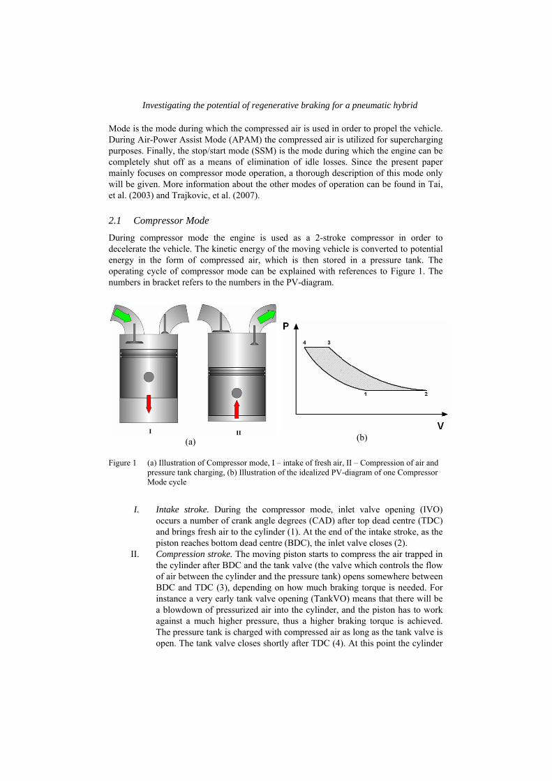
Investigating the potential of regenerative braking for a pneumatic hybrid
Mode is the mode during which the compressed air is used in order to propel the vehicle. During Air-Power Assist Mode (APAM) the compressed air is utilized for supercharging purposes. Finally, the stop/start mode (SSM) is the mode during which the engine can be completely shut off as a means of elimination of idle losses. Since the present paper mainly focuses on compressor mode operation, a thorough description of this mode only will be given. More information about the other modes of operation can be found in Tai, et al. (2003) and Trajkovic, et al. (2007).
2.1 Compressor Mode
During compressor mode the engine is used as a 2-stroke compressor in order to decelerate the vehicle. The kinetic energy of the moving vehicle is converted to potential energy in the form of compressed air, which is then stored in a pressure tank. The operating cycle of compressor mode can be explained with references to Figure 1. The numbers in bracket refers to the numbers in the PV-diagram.
(a)
(b)
Figure 1 (a) Illustration of Compressor mode, I – intake of fresh air, II – Compression of air and pressure tank charging, (b) Illustration of the idealized PV-diagram of one Compressor Mode cycle
I. Intake stroke. During the compressor mode, inlet valve opening (IVO)
occurs a number of crank angle degrees (CAD) after top dead centre (TDC) and brings fresh air to the cylinder (1). At the end of the intake stroke, as the piston reaches bottom dead centre (BDC), the inlet valve closes (2).
II. Compression stroke. The moving piston starts to compress the air trapped in the cylinder after BDC and the tank valve (the valve which controls the flow of air between the cylinder and the pressure tank) opens somewhere between BDC and TDC (3), depending on how much braking torque is needed. For instance a very early tank valve opening (TankVO) means that there will be a blowdown of pressurized air into the cylinder, and the piston has to work against a much higher pressure, thus a higher braking torque is achieved. The pressure tank is charged with compressed air as long as the tank valve is open. The tank valve closes shortly after TDC (4). At this point the cylinder

is filled with compressed air at the same pressure level as the air in the pressure tank. As the piston moves towards BDC, the compressed air expends and the intake valve opens (1) when ambient pressure is reached in the cylinder.
2.2 Variable Valve Actuation
The description of the compressor mode above implies a need for a variable valve actuating (VVA) system. The VVA system used in the study described in present paper is an electro pneumatic valve actuating (EPVA) system. The EPVA uses compressed air in order to drive the valves and the motion of the valves are controlled by a combination of electronics and hydraulics. The system is a fully variable valve actuating system, i.e. valve timing, duration and lift height can be controlled independently of each other. A thorough description of the EPVA system can be found in the work of Trajkovic, et al. (2006) while Ma, et al. (2006) presents a dynamic model of the EPVA system.
2.3 Tank Valve
In order to run the engine as a pneumatic hybrid powertrain, a pressure tank has to be connected to the engine. There is also a need for a valve dedicated to control the flow of air into and out from the pressure tank. There are numerous suggested solutions to how such a way should be constructed. Tai, et al. (2003) describes an intake air switching system in which one inlet valve per cylinder is feed by either fresh intake air or compressed air form the pressure tank. Andersson, et al. (2005) describes a dual valve system, where one of the intake ports has two valves, one of whom is connected to the pressure tank. Dönitz, et al. (2009), presents a solution where an extra valve is introduced to the cylinder head in addition to the conventional valve train. In the study described in present paper, a different and simpler solution has been chosen where one of the existing inlet valves has been converted to operate as a tank valve. Since the engine used the study has separated inlet ports, there will be no interference between the intake system and the compressed air system. The drawback with this solution is that there will be a significant reduction in peak power due to limited air flow into the cylinder during the intake stroke. Another drawback is that the ability to generate and control swirl for good combustion will be reduced.
3 Load Control during Compressor Mode
An important aspect of the pneumatic hybrid concept is its ability to control the amount of braking torque at a specific time. A desired torque should be achievable whatever the pressure level in the tank is. For this purpose, a control strategy has been adopted, that controls the pneumatic hybrid powertrain load during compressor mode and air-motor mode at different tank pressures. Figure 2 illustrates the closed-loop controller for compressor mode load control. The structure consists of a feed-forward filter and a PID controller. The feed-forward filter contains data about valve timings at different loads acquired from steady-state experiments. It takes the measured load from previous cycle as argument and based on this, it outputs proper steady-state valve timings at current
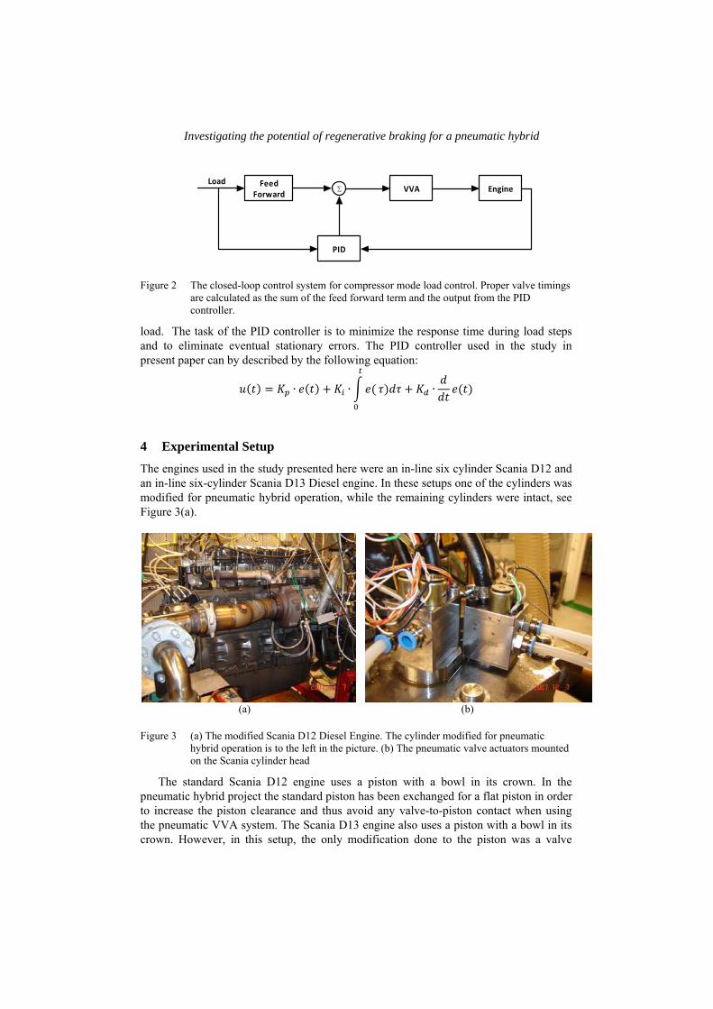
Investigating the potential of regenerative braking for a pneumatic hybrid
Figure 2 The closed-loop control system for compressor mode load control. Proper valve timings are calculated as the sum of the feed forward term and the output from the PID controller.
load. The task of the PID controller is to minimize the response time during load steps and to eliminate eventual stationary errors. The PID controller used in the study in present paper can by described by the following equation:
∙ ∙ ∙
4 Experimental Setup
The engines used in the study presented here were an in-line six cylinder Scania D12 and an in-line six-cylinder Scania D13 Diesel engine. In these setups one of the cylinders was modified for pneumatic hybrid operation, while the remaining cylinders were intact, see Figure 3(a).
(a) (b)
Figure 3 (a) The modified Scania D12 Diesel Engine. The cylinder modified for pneumatic hybrid operation is to the left in the picture. (b) The pneumatic valve actuators mounted on the Scania cylinder head
The standard Scania D12 engine uses a piston with a bowl in its crown. In the pneumatic hybrid project the standard piston has been exchanged for a flat piston in order to increase the piston clearance and thus avoid any valve-to-piston contact when using the pneumatic VVA system. The Scania D13 engine also uses a piston with a bowl in its crown. However, in this setup, the only modification done to the piston was a valve
VVA EngineFeed
Forward
PID
Load

pocket for the tank valve. The reason is that the engine will be used for fired operation later in the pneumatic hybrid project and therefore there is a need for the bowl to achieve satisfying diesel combustion. Some engine specifications can be found in Table 1.
Table 1 Geometric properties of the Scania D12 and D13 diesel engine
Scania D12 Scania D13
Displaced Volume (x6) 1966 cm3 2100 cm3
Bore 127.5 mm 130 mm
Stroke 154 mm 160 mm
Connecting Rod Length 255 mm
Number of Valves 4
Compression Ratio 18:1 17.2
Piston type Flat Bowl
Inlet valve diameter 45 mm
Tank valve diameter 28
Piston clearance 7.3 mm 0.9 mm The standard camshaft has been removed from both engines, and the engine valves
are instead actuated by the pneumatic VVA system described earlier. Figure 3(b) shows the pneumatic valve actuators mounted on top of the Scania D12 cylinder head. The same setup has been used on the Scania D13 engine. In Table 2, some valve operating parameters are shown. The maximum valve lift height has been limited to 7 mm in order to avoid valve-to-piston contact and thus prevent engine failure. The standard valve springs have been exchanged for less stiff springs in order to reduce the energy required to operate the valves.
Both engines have two separated inlet ports and therefore they are suitable to use with the pneumatic hybrid since there will be no interference between the intake air and the compressed air. One of the inlet valves was therefore converted to a tank valve. The exhaust valves were deactivated throughout the study presented here because no fuel was injected and thus there was no need for exhaust gas venting.
The pressure tank used in the study presented here was an AGA 50 liter pressure tank normally used for storage of different types of gases at pressures up to 200 bar. It is connected to the cylinder head by metal tubing. The size of the tank in present study was selected based on availability rather than optimality.
Table 2 Valve operating parameters
Inlet valve supply pressure 4 bar
Tank valve supply pressure 6 bar
Hydraulic brake pressure 4 bar
Inlet valve spring preloading 100 N
Tank valve spring preloading 340 N
Maximum valve lift 7 mm

Investigating the potential of regenerative braking for a pneumatic hybrid
5 Results
The Compressor Mode can be done mainly in three different ways: with emphasis on maximum efficiency, maximum brake torque generation and lastly a combination of both. The first two subsections focus on CM operation with maximum compressor mode efficiency, both with theoretically calculated valve timings and with valve timings retrieved from experimental data. The third subsection focuses mainly on the parameters influencing the compressor mode performance while the subsection deals with closed-loop control of the load during compressor mode.
5.1 Compressor Mode Operation with Theoretically Calculated Valve Timings
One way of running CM operation with focus on maximum efficiency is to use theoretically calculated valve timings. As described earlier in present paper, according to idealized CM operation the TankVO should occur when the pressure inside the cylinder equals the pressure in the tank. This means that there will be no blow down or over-compression of pressurized air. In this part of the study, the TankVO was controlled by an open-loop controller based on the polytropic compression law:
where p1 corresponds to the pressure at BDC and p2 is the pressure at any point in the cycle. V1 is the maximum volume in the cylinder and V2 is the cylinder volume at cylinder pressure p2. By setting p2 equal to the tank pressure, the volume at the given pressure can be calculated. By comparing V2 to a precalculated CAD-resolved volume trace, proper valve timings can be determined. The same strategy can also be used to determine TankVC and IVO.
The advantage with this strategy is that the valve timings are determined in a very simple way and it is easy to implement in the control program. However, there are some drawbacks with this strategy. On is that the polytropic exponent, κ, depends on heat losses and setting it to a constant value introduces some errors in the TankVO control algorithm. Another drawback is that the strategy doesn’t take the dynamics of the system, such as pressure wave propagation into consideration.
Figure 4 PV-diagram of the cylinder pressure (left) and tank pressure (right) of one CM cycle at a tank pressure of 6 bar and an engine speed of 600 rpm
0 0.5 1 1.5 2 2.50
2
4
6
8
10
12
Cylinder Volume [dm3]
Cyl
ind
er
Pre
ssu
re [b
ar]
TVC TVO
IVO IVC
Tank Pressure = 6 barTVO = 50 CAD BTDCTVC = 6 CAD ATDCIVO = 49 CAD ATDCIVC = 180 CAD ATDC
-150 -100 -50 0 50 100 1504
4.5
5
5.5
6
6.5
7
7.5
8
CAD [ATDC]
Ta
nk
Pre
ssu
re [b
ar]
TVO
TVC
IVO
IVC

Int. J.Powertrains , Vol. 1, No. 1, 2011 8
Copyright © 200x Inderscience Enterprises Ltd.
Figure 5 Negative IMEP and mean tank pressure during transient CM operation as a function of engine cycle number at an engine speed of 600 rpm
Figure 4 show a PV diagram of the in-cylinder pressure and tank pressure during one engine cycle. According to the idealized PV-diagram shown in Figure 1(b), the pressure between TVO and TVC should be constant. However, the PV-diagram in Figure 4 shows no such isobaric event during real engine testing. The reason is that the flow over the tank valve becomes very restricted which is also known as choked flow. This will therefore lead to an overshoot in in-cylinder pressure compared to the idealized conditions. This phenomenon highly depends on the size of the tank valve, tank pressure and engine speed, which will be demonstrated later on in present paper.
Figure 5 shows the generated negative indicated mean effective pressure (IMEP) and accumulated tank pressure during 800 consecutive engine cycles. The valve timings are controlled according to the strategy described earlier in current subsection. One thing that can be noted from the figure is that the negative IMEP at first increases rapidly but then it starts to move towards an almost constant value. The reason for this behaviour is the choice of valve timings and can be explained with the help of Figure 6. When the pressure in the tank is low, TankVO occurs early in the cycle. As the tank pressure starts to increase, TankVO moves away from BDC and towards TDC. At low tank pressures the, difference in TankVO for a given pressure difference, is much larger than at a high tank pressure for the same pressure difference. A large change in valve timing will lead to
Figure 6 Illustration of how the change in CAD for a change in pressure by 1 bar changes with increasing pressure.
0 200 400 600 8000
0.8
1.6
2.4
3.2
4
Ne
ga
tive
IME
P [b
ar]
Number of Engine Cycles [-]
0 200 400 600 8000
5
10
15
20
25
Ta
nk
Pre
ssu
re [b
ar]
Negative IMEPTank Pressure
-70 -60 -50 -40 -30 -20 -10
2
4
6
8
10
12
14
16
18
20
CAD [ATDC]
Cyl
ind
er
Pre
ssu
re [b
ar]
Δp=1 bar
Δp=1 bar

Investigating the potential of regenerative braking for a pneumatic hybrid
a large change in IMEP while a small change in TankVO will only have a modest influence on IMEP.
5.2 Optimized Compressor Mode Operation The strategy with theoretically calculated valve timings have some flaws as described
above and this can lead to inaccurate valve timing when taking maximum compressor mode efficiency in consideration. In order to avoid this problem, proper valve timings can be determined experimentally. In present study a method to optimize the compressor mode will be presented. The main idea with this method is to find optimal valve timing at a given tank pressure and, in order to do that, the tank pressure needs to be constant throughout the entire testing interval (steady state). With a pressure relief valve connected to the tank, it is possible to control the pressure level in the system.
(a) (b)
Figure 7 Steady-state optimization of the Compressor Mode at an engine speed of 600 rpm; (a) Negative IMEP obtained during steady-state CM as a function of TankVO for different tank pressures; (b) Optimal TankVO and corresponding negative IMEP for Compressor Mode operation as a function of tank pressure.
Figure 7(a) shows a TankVO optimization sweep at various steady-state tank pressures. It can clearly be seen how negative IMEP is affected by TankVO timing during optimization of CM. Figure 7(a) indicates that there is an optimal TankVO timing for every tank pressure when taking highest compressor mode efficiency in consideration; highest efficiency corresponds to the minimum in each curve. This means that it takes less power to compress the inducted air at this point that at any other point on the curve at a given tank pressure. If higher brake torque is needed, the efficiency has to be sacrificed The reason why negative IMEP increases at early TankVO is that when the tank valve opens earlier than optimal, there will be a blowdown of compressed air into the cylinder due to the fact that the pressure level in the cylinder is lower than the pressure level in the pressure tank. At a certain premature TankVO, negative IMEP will dramatically increase with increasing tank pressure, due to a larger pressure level difference between the cylinder and the pressure tank. Trajkovic et al. (2009) demonstrated that if maximum braking torque is desired, the TankVO should open at BDC. In this way it was possible to achieve over 6000 Nm of braking torque for a 16-liter heavy-duty truck engine.
0501001502002
3
4
5
6
7
TankVO [CAD BTDC]
Ne
ga
tive
IME
P [b
ar]
4 bar10 bar15 bar21 bar
3 6 9 12 15 18 21
20
35
50
65
80
Ta
nkV
O [C
AD
BT
DC
]
Tank Pressure [bar]
3 6 9 12 15 18 211.5
2
2.5
3
3.5
Ne
ga
tive
IME
P [b
ar]
TankVONegative IMEP

Figure 7(b) shows the how optimal TankVO and corresponding negative IMEP varies with increasing tank pressure. The reason why the negative IMEP decreases after a tank pressure of approximately 14 bar is most likely due to system dynamics in the form of pressure wave propagation through the system. A more in-depth look on this matter will be presented later in present paper.
In Figure 8, the results from transient compressor mode operation during 800 consecutive engine cycles can be seen. The results contain data from compressor mode operation with both theoretical valve timing and optimized valve timing. Initially, negative IMEP for the theoretical case is similar to the negative IMEP for the optimized case, but after about 300 engine cycles negative IMEP for the optimized case remains reasonably constant while negative IMEP for the theoretical case continues to increase throughout the rest of the experiment. Even though a higher efficiency has been achieved with the optimized case, the final tank pressure after 800 engine cycles is lower by 0.2 bar compared to the theoretical case. This behaviour can once again be explained by the dynamics of the system and a more thorough investigation of this occurrence will be presented later in present paper.
Figure 8 Comparison of negative IMEP for theoretical and optimized valve timings as a function of engine cycle number during CM operation.
5.3 Parametric Study of Compressor Mode The main goal during compressor mode is always to, at any given situation maximize
the charging of the pressure tank. In previous subsection it could be noticed that even though the valve timings were optimized with regards to maximum compressor mode efficiency, the tank pressure decreased compared to the less accurate theoretical approach. This leads to the conclusion that there are some underlying phenomena affecting the performance of the compressor mode. The purpose of current subsection is to investigate different parameters in order to understand their influence on the compressor mode performance. The relevant parameters which will be investigated are the tank valve diameter, tank valve opening and closing, and inlet valve opening. There are some more parameters influencing the performance of compressor mode, but their influence is small compared to the once mentioned above and they are therefore not dealt with here.
0 200 400 600 8000
0.5
1
1.5
2
2.5
3
3.5
Number of Engine Cycles
Ne
ga
tive
IME
P [b
ar]
Theoretical Valve TimingFinal TankP = 21.2 barOptimized Valve TimingFinal TankP = 21.0 bar

Investigating the potential of regenerative braking for a pneumatic hybrid
5.3.1 Tank Valve Diameter The importance of proper tank valve diameter high efficiency compressor mode
operation has been demonstrated by Trajkovic et al. (2008), where two different tank valves configurations with different valve diameters were tested. A small tank valve diameter will restrict the air flow into and out from the pressure tank with high pressure losses as a result. During compressor mode operation this will show as an overshoot in in-cylinder pressure. By maximizing the tank valve diameter the restriction of the flow can be held to a minimum. Figure 9 show how the in-cylinder pressure at two different engine speeds and a tank pressure of 10 bar. It can clearly be seen how the overshoot in in-cylinder pressure decreases with increasing tank valve diameter. Also the engine speed plays an important role here. At an engine speed of 600 rpm, the overshoot with the 16 mm tank valve is larger compared to the other two valve configurations but still at reasonable levels. However, as the engine speed increases to 1500 rpm, the in-cylinder pressure overshoots by more than 10 bar compared to the tank pressure for the 16 mm tank valve, which implies that the flow into the tank is extremely restricted. In Figure 10
(a) (b)
Figure 9 Cylinder pressure for various tank valve diameters at the engine speeds 600 rpm (a) and 1500 rpm (b). Tank pressure = 10 bar.
(a) (b)
Figure 10 Cylinder pressure with a tank valve diameter of 16 mm (a) and 32 mm (b), respectively, at various engine speeds
-50 0 500
5
10
15
20
25
CAD [ATDC]
Cyl
ind
er
Pre
ssu
re [b
ar]
=16 mm=24 mm=32 mm
-50 0 500
5
10
15
20
25
CAD [ATDC]
Cyl
ind
er
Pre
ssu
re [b
ar]
=16 mm=24 mm=32 mm
-50 0 500
5
10
15
20
25
CAD [ATDC]
Cyl
ind
er
Pre
ssu
re [b
ar]
600 rpm900 rpm1200 rpm1500 rpm
-50 0 500
5
10
15
20
25
CAD [ATDC]
Cyl
ind
er
Pre
ssu
re [b
ar]
600 rpm900 rpm1200 rpm1500 rpm

it can be more clearly seen how the engine speed affects the overshoot in in-cylinder pressure for a 16 mm tank valve and a 32 mm tank valve, respectively.
A direct measure of the performance of the compressor mode is the mass flow of compressed air into the tank. The higher the mass flow is, the higher the increase in tank pressure will be. In Figure 11 the mass flow of compressed air into the tank for different engine speeds and tank valve diameters can be seen. At low engine speeds, the mass flow is almost constant independently of valve diameter. The reason is that, at low piston speeds, there will be enough time for the compressed air to flow into the tank, even though it is restricted for the smaller tank valve diameters. However at higher engine speeds the available time for venting the cylinder from compressed air decreases and it can clearly be seen that the tank valve diameter of 16 mm limits the mass flow severely compared to the other tank valve configurations. It is also very interesting to see that with the 32 mm tank valve, the mass flow becomes almost constant above 900 rpm, see Figure 11(b).
(a) (b)
Figure 11 (a) Mass flow of compressed air into the tank as a function of tank valve diameter for various engine speeds, (b) Mass flow of compressed air into the tank as a function of engine speed for two different tank valve diameters. Tank pressure = 10 bar
In The results shown so far in present subsection has all been retrieved during steady-stat Compressor Mode operation. In Figure 12, the results from transient Compressor Mode operation during 800 consecutive engine cycles are shown. The results at 600 rpm are in analogy with what has previously been shown for steady-state operation. In Figure 11(a) the mass flow was almost independent of valve diameter at 600 rpm, and
Table 3, IMEP and mass flow for two different valve diameters and two different engine speeds are presented. IMEP represents the energy that the engine consumes in order to compress the air to a specific pressure level and the mass flow represents the energy that goes into the pressure tank. For best performance, the energy consumed should be at a minimum while the energy transferred to the tank should be at a maximum. In other words, the goal is to lower the IMEP and in the same time maximize the mass flow of compressed air into the tank. At 600 rpm, it can be seen that with the 32 mm tank valve IMEP is lower and mass flow is slightly higher compared to the case with the 16 mm tank valve, thus the Compressor Mode performance will be better with the larger
15 20 25 30 351.3
1.4
1.5
1.6
1.7
1.8
Tank Valve Diameter [mm]
Ma
ss fl
ow
[g/c
ycle
]
600 rpm900 rpm1200 rpm1500 rpm
600 800 1000 1200 1400 16001.3
1.4
1.5
1.6
1.7
1.8
Engine Speed [rpm]
Ma
ss fl
ow
[g/c
ycle
]
=16 mm=32 mm

Investigating the potential of regenerative braking for a pneumatic hybrid
valve setup. At 1500 rpm, the difference between the two tank valve configurations becomes much higher, indicating the advantage of using a large tank valve diameter.
The results shown so far in present subsection has all been retrieved during steady-stat Compressor Mode operation. In Figure 12, the results from transient Compressor Mode operation during 800 consecutive engine cycles are shown. The results at 600 rpm are in analogy with what has previously been shown for steady-state operation. In Figure 11(a) the mass flow was almost independent of valve diameter at 600 rpm, and
Table 3 The influence of tank valve diameter and engine speed on IMEP and mass flow during Compressor Mode operation
Engine speed [rpm]
ø [mm]IMEP [bar]
Mflow [g/cycle]
600 16 2.49 1.77
32 2.16 1.78
1500 16 3.25 1.34
32 2.73 1.72
this behaviour can once again be seen during transient operation in Figure 12(a). At 1500 rpm the mass flow is comparable to what has been shown for steady state operation in Figure 11(a). One thing that requires attention is that even though the mass flow has decreased at1500 rpm compared to at 600 rpm, the tank pressure has increased. The explanation for
(a) (b)
Figure 12 Mass flow and tank pressure as a function of number of engine cycles for two different valve configurations during transient CM operation at an engine speed of 600 rpm (a) and 1200 rpm (b), respectively.
this behaviour is most likely that, at a higher engine speed there will be less time for heat transfer to occur between the hot compressed air and the system it flows through. This
0 200 400 600 8000.2
1
1.8
2.6
3.4
Ma
ss F
low
[g/c
ycle
]
Number of Engine Cycles [-]
0 200 400 600 8000
6
12
18
24
0 200 400 600 8000
6
12
18
24
=16 mm=32 mm
0 200 400 600 8000.2
1
1.8
2.6
3.4
Ma
ss F
low
[g/c
ycle
]
Number of Engine Cycles [-]
0 200 400 600 8000
6
12
18
24
Ta
nk
Pre
ssu
re [b
ar]
0 200 400 600 8000
6
12
18
24
=16 mm=32 mm

means that the temperature in the pressure tank will be higher compared to the case at 600 rpm, with higher pressure in the tank as a result.
5.3.2 Tank Valve Opening The TankVO is probably the most important parameter influencing the performance
of the Compressor Mode operation. It directly determines how much brake torque will be generated at a given tank pressure. Figure 13 shows the results IMEP and mass flow from a TankVO sweep at two engine speeds, 600 and 1200 rpm. As mentioned earlier in section 5.2, optimal TankVO with regards to maximum efficiency will occur where IMEP is at a minimum, in this case at about 40 CAD BTDC. At this optimal point the cylinder pressure will be about equal to the tank pressure. If TankVO is advanced from the optimal point, IMEP will start to increase due to excessive compression of the air in the cylinder. Retarding the TankVO from the optimal point also leads to an increase in IMEP. The reason is that, when TankVO opens earlier than at the optimal point, there will be a blowdown of compressed air into the cylinder due to the fact that the in-cylinder pressure will be below the pressure in the tank. By retarding TankVO, the amount of braking torque generated can be controlled. Highest brake torque will be achieved when TankVO occurs at BDC. Between 180 and 70 CAD BTDC, it can be noticed that IMEP is higher for the case at 600 rpm compared to the case at 1200 rpm. The main reason for this behaviour is that at a higher engine speed, there will be less time for the previously described blowdown process to occur and thereby its effect on IMEP will be less.
Figure 13 Mass flow and IMEP as a function of TankVO at a tank pressure of 10 bar and two different engine speeds.
The other variable shown in Figure 13 is the mass flow of compressed air into the tank. It can be observed that the mass flow at the optimum point (40 CAD BTDC) and at an engine speed of 600 rpm is not at a maximum. The maximum mass flow instead occurs with a TankVO at about 130 CAD BTDC. However, at 1200 rpm the maximum air flow occurs in the vicinity of the optimal point. This phenomenon can be explained by pressure wave propagation in the pipeline connecting the tank to the cylinder head. For instance, a pressure wave can propagate back into the cylinder while the tank valve is open which can lead to a less than optimal charging of the tank. This propagation of pressure waves and their effect on the Compressor Mode performance will be discussed in more detail in section 5.3.5.
-200 -150 -100 -50 01
1.2
1.4
1.6
1.8
2
Ma
ss F
low
[g/c
ycle
]
TankVO [CAD ATDC]
-200 -150 -100 -50 02
4
6
8
10
12
Ne
ga
tive
IME
P [b
ar]
-200 -150 -100 -50 02
4
6
8
10
12
600 rpm1200 rpm

Investigating the potential of regenerative braking for a pneumatic hybrid
Figure 14 and Figure 15 display IMEP, mass flow and tank pressure for three different TankVO during transient Compressor Mode operation at two different engine speeds, 600 and 1200 rpm. The results follow the same trend as shown for the steady-state operation shown in Figure 13. In analogy to Figure 13, IMEP increases with retarded TankVO at both engine speeds, see Figure 14(a) and Figure 15(b). At 1200 rpm the mass flow has decreased for early TankVO and consequently the tank pressure has also decreased compared to the case at 600 rpm. For late TankVO (80 CAD BTDC) the mass flow at 600 and 1200 rpm, respectively, is almost the same, and hence similar pressure curves are achieved.
(a) (b)
Figure 14 Various parameters as a function of engine cycles for three different TankVO at an engine speed of 600 rpm, (a) Negative IMEP, (b) Mass flow and tank pressure.
(a) (b)
Figure 15 Various parameters as a function of engine cycles for three different TankVO at an engine speed of 1200 rpm, (a) Negative IMEP, (b) Mass flow and tank pressure.
5.3.3 Tank Valve Closing
TankVC is also a very important parameter influencing the Compressor Mode performance. It determines when the charging of the pressure tank should end. Ideally the TankVC should occur during the expansion stroke at the moment the pressure in the
0 200 400 600 8000
5
10
15
20
25
Engine cycles [-]
Ne
ga
tive
IME
P [b
ar]
TankVO=-180TankVO=-130TankVO=-80
0 200 400 600 8000.2
1
1.8
2.6
3.4
Ma
ss F
low
[g/c
ycle
]
Number of Engine Cycles [-]
0 200 400 600 8000
6
12
18
24
Ta
nk
Pre
ssu
re [b
ar]
0 200 400 600 8000
6
12
18
24
0 200 400 600 8000
6
12
18
24
TankVO=180TankVO=130TankVO=80
0 200 400 600 8000
5
10
15
20
25
Engine cycles [-]
Ne
ga
tive
IME
P [b
ar]
TankVO=-180TankVO=-130TankVO=-80
0 200 400 600 8000.2
1
1.8
2.6
3.4
Ma
ss F
low
[g/c
ycle
]
Number of Engine Cycles [-]
0 200 400 600 8000
6
12
18
24
Ta
nk
Pre
ssu
re [b
ar]
0 200 400 600 8000
6
12
18
24
0 200 400 600 8000
6
12
18
24TankVO=180TankVO=130TankVO=80
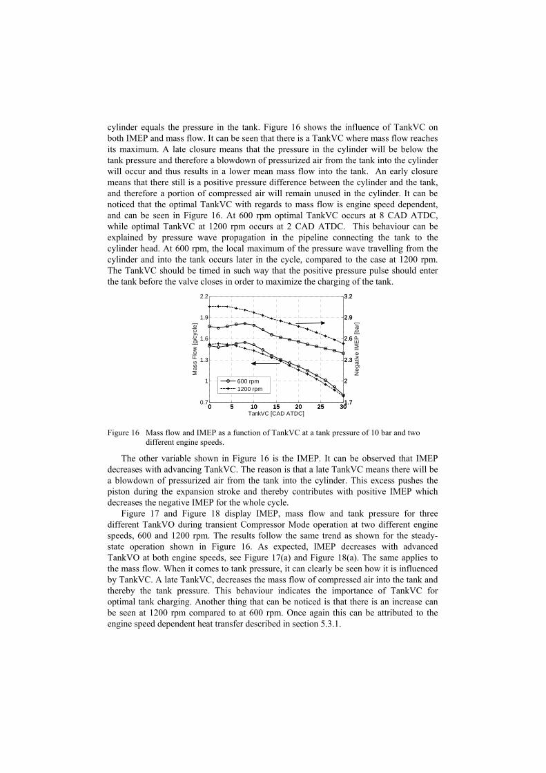
cylinder equals the pressure in the tank. Figure 16 shows the influence of TankVC on both IMEP and mass flow. It can be seen that there is a TankVC where mass flow reaches its maximum. A late closure means that the pressure in the cylinder will be below the tank pressure and therefore a blowdown of pressurized air from the tank into the cylinder will occur and thus results in a lower mean mass flow into the tank. An early closure means that there still is a positive pressure difference between the cylinder and the tank, and therefore a portion of compressed air will remain unused in the cylinder. It can be noticed that the optimal TankVC with regards to mass flow is engine speed dependent, and can be seen in Figure 16. At 600 rpm optimal TankVC occurs at 8 CAD ATDC, while optimal TankVC at 1200 rpm occurs at 2 CAD ATDC. This behaviour can be explained by pressure wave propagation in the pipeline connecting the tank to the cylinder head. At 600 rpm, the local maximum of the pressure wave travelling from the cylinder and into the tank occurs later in the cycle, compared to the case at 1200 rpm. The TankVC should be timed in such way that the positive pressure pulse should enter the tank before the valve closes in order to maximize the charging of the tank.
Figure 16 Mass flow and IMEP as a function of TankVC at a tank pressure of 10 bar and two different engine speeds.
The other variable shown in Figure 16 is the IMEP. It can be observed that IMEP decreases with advancing TankVC. The reason is that a late TankVC means there will be a blowdown of pressurized air from the tank into the cylinder. This excess pushes the piston during the expansion stroke and thereby contributes with positive IMEP which decreases the negative IMEP for the whole cycle.
Figure 17 and Figure 18 display IMEP, mass flow and tank pressure for three different TankVO during transient Compressor Mode operation at two different engine speeds, 600 and 1200 rpm. The results follow the same trend as shown for the steady-state operation shown in Figure 16. As expected, IMEP decreases with advanced TankVO at both engine speeds, see Figure 17(a) and Figure 18(a). The same applies to the mass flow. When it comes to tank pressure, it can clearly be seen how it is influenced by TankVC. A late TankVC, decreases the mass flow of compressed air into the tank and thereby the tank pressure. This behaviour indicates the importance of TankVC for optimal tank charging. Another thing that can be noticed is that there is an increase can be seen at 1200 rpm compared to at 600 rpm. Once again this can be attributed to the engine speed dependent heat transfer described in section 5.3.1.
0 5 10 15 20 25 300.7
1
1.3
1.6
1.9
2.2
Ma
ss F
low
[g/c
ycle
]
TankVC [CAD ATDC]
0 5 10 15 20 25 301.7
2
2.3
2.6
2.9
3.2
Ne
ga
tive
IME
P [b
ar]
0 5 10 15 20 25 301.7
2
2.3
2.6
2.9
3.2
600 rpm1200 rpm

Int. J.Powertrains , Vol. 1, No. 1, 2011 17
Copyright © 200x Inderscience Enterprises Ltd.
(a) (b)
Figure 17 Various parameters as a function of engine cycles for three different TankVC at an engine speed of 600 rpm, (a) Negative IMEP, (b) Mass flow and tank pressure.
(a) (b)
Figure 18 Various parameters as a function of engine cycles for three different TankVC at an engine speed of 1200 rpm, (a) Negative IMEP, (b) Mass flow and tank pressure.
5.3.4 Inlet Valve Opening
The role of the inlet valve during Compressor Mode operation is to admit a fresh charge of air during the end of the expansion stroke. The inlet valve should open when the pressure in the cylinder during the expansion stroke reaches ambient pressure. A too late IVO will lead to a decrease in in-cylinder pressure below ambient pressure and thus vacuum is created which is an energy consuming process. When the IVO finally occurs, the vacuum is cancelled by the induction of fresh air into the cylinder and thereby the vacuum previously created cannot be used as an upward-acting force on the piston as it moves towards TDC. The influence of IVO on mass flow and IMEP during steady-state operation for two engine speeds can be seen in Figure 19. It can be observed that there is an optimal IVO where mass flow reaches a maximum at both engine speeds. There are two different effects occurring when IVO is retarded or advanced, respectively, away from optimal IVO. If IVO occurs too early, the pressure in the cylinder will be above
0 200 400 600 8001.5
2
2.5
3
3.5
4
Engine cycles [-]
Ne
ga
tive
IME
P [b
ar]
TankVC=0TankVC=15TankVO=30
0 200 400 600 8000.2
1
1.8
2.6
3.4
Ma
ss F
low
[g/c
ycle
]
Number of Engine Cycles [-]
0 200 400 600 8000
6
12
18
24
Ta
nk
Pre
ssu
re [b
ar]
0 200 400 600 8000
6
12
18
24
0 200 400 600 8000
6
12
18
24
TankVC=0TankVC=15TankVC=30
0 200 400 600 8002
2.5
3
3.5
4
4.5
Engine cycles [-]
Ne
ga
tive
IME
P [b
ar]
TankVC=0TankVC=15TankVO=30
0 200 400 600 8000.2
1
1.8
2.6
3.4
Ma
ss F
low
[g/c
ycle
]
Number of Engine Cycles [-]
0 200 400 600 8000
6
12
18
24
Ta
nk
Pre
ssu
re [b
ar]
0 200 400 600 8000
6
12
18
24
0 200 400 600 8000
6
12
18
24
TankVC=0TankVC=15TankVC=30
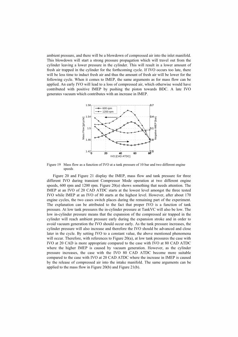
ambient pressure, and there will be a blowdown of compressed air into the inlet manifold. This blowdown will start a strong pressure propagation which will travel out from the cylinder leaving a lower pressure in the cylinder. This will result in a lower amount of fresh air trapped in the cylinder for the forthcoming cycle. If IVO occurs too late, there will be less time to induct fresh air and thus the amount of fresh air will be lower for the following cycle. When it comes to IMEP, the same arguments as for mass flow can be applied. An early IVO will lead to a loss of compressed air, which otherwise would have contributed with positive IMEP by pushing the piston towards BDC. A late IVO generates vacuum which contributes with an increase in IMEP.
Figure 19 Mass flow as a function of IVO at a tank pressure of 10 bar and two different engine speeds
Figure 20 and Figure 21 display the IMEP, mass flow and tank pressure for three different IVO during transient Compressor Mode operation at two different engine speeds, 600 rpm and 1200 rpm. Figure 20(a) shows something that needs attention. The IMEP at an IVO of 20 CAD ATDC starts at the lowest level amongst the three tested IVO while IMEP at an IVO of 80 starts at the highest level. However, after about 170 engine cycles, the two cases switch places during the remaining part of the experiment. The explanation can be attributed to the fact that proper IVO is a function of tank pressure. At low tank pressures the in-cylinder pressure at TankVC will also be low. The low in-cylinder pressure means that the expansion of the compressed air trapped in the cylinder will reach ambient pressure early during the expansion stroke and in order to avoid vacuum generation the IVO should occur early. As the tank pressure increases, the cylinder pressure will also increase and therefore the IVO should be advanced and close later in the cycle. By setting IVO to a constant value, the above mentioned phenomena will occur. Therefore, with references to Figure 20(a), at low tank pressures the case with IVO at 20 CAD is more appropriate compared to the case with IVO at 80 CAD ATDC where the higher IMEP is caused by vacuum generation. However, as the cylinder pressure increases, the case with the IVO 80 CAD ATDC become more suitable compared to the case with IVO at 20 CAD ATDC where the increase in IMEP is caused by the release of compressed air into the intake manifold. The same arguments can be applied to the mass flow in Figure 20(b) and Figure 21(b).
0 20 40 60 801.42
1.46
1.5
1.54
1.58
Ma
ss F
low
[g/c
ycle
]
IVO [CAD ATDC]
0 20 40 60 802.5
2.8
3.1
3.4
3.7
Ne
ga
tive
IME
P [b
ar]
0 20 40 60 802.5
2.8
3.1
3.4
3.7600 rpm1200 rpm

Int. J.Powertrains , Vol. 1, No. 1, 2011 19
Copyright © 200x Inderscience Enterprises Ltd.
(a) (b)
Figure 20 Various parameters as a function of engine cycles for three different TankVC at an engine speed of 600 rpm, (a) Negative IMEP, (b) Mass flow and tank pressure.
(a) (b)
Figure 21 Various parameters as a function of engine cycles for three different TankVC at an engine speed of 600 rpm, (a) Negative IMEP, (b) Mass flow and tank pressure.
5.3.5 The Effects of Pressure Wave Propagation on Compressor Mode operation
It is widely known that the geometry of the intake and exhaust lines has a great influence on the gas wave motion, which can be utilized for supercharging of the engine. Knowledge of pressure wave propagation is also important for the pneumatic hybrid. If the pipeline connecting the pressure tank to the engine is poorly tuned, a pressure wave can propagate back into the cylinder while the tank valve is open which can lead to a less than optimal charging of the tank. Figure 22 shows the mass flow as a function of both IMEP and tank pressure. It can be seen that the isolines show a wave-like behaviour. At low tank pressures the isolines are almost parallel with the y-axis. In other words, the mass flow at low tank pressures is almost independent of the load. However, at higher tank pressures the isolines transforms into wave-like lines. This behaviour can be explained with pressure wave propagation in the pipeline connecting the pressure tank with the cylinder head.
0 200 400 600 8001.5
2
2.5
3
3.5
4
4.5
5
Number of Engine Cycles [-]
Ne
ga
tive
IME
P [b
ar]
IVO=20IVO=50IVO=80
0 200 400 600 8000.2
1
1.8
2.6
3.4
Ma
ss F
low
[g/c
ycle
]
Number of Engine Cycles [-]
0 200 400 600 8000
6
12
18
24
Ta
nk
Pre
ssu
re [b
ar]
0 200 400 600 8000
6
12
18
24
0 200 400 600 8000
6
12
18
24
IVO=20IVO=50IVO=80
0 200 400 600 8002
2.5
3
3.5
4
4.5
5
Number of Engine Cycles [-]
Ne
ga
tive
IME
P [b
ar]
IVO=20IVO=50IVO=80
0 200 400 600 8000.2
1
1.8
2.6
3.4
Ma
ss F
low
[g/c
ycle
]
Number of Engine Cycles [-]
0 200 400 600 8000
6
12
18
24
Ta
nk
Pre
ssu
re [b
ar]
0 200 400 600 8000
6
12
18
24
0 200 400 600 8000
6
12
18
24
IVO=20IVO=50IVO=80
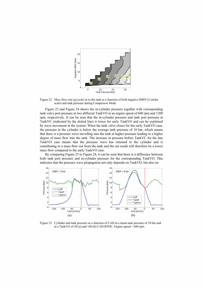
Figure 22 Mass flow rate (g/cycle) in to the tank as a function of both negative IMEP (2-stroke scale) and tank pressure during Compressor Mode
Figure 23 and Figure 24 shows the in-cylinder pressure together with corresponding tank valve port pressure at two different TankVO at an engine speed of 600 rpm and 1200 rpm, respectively. It can be seen that the in-cylinder pressure and tank port pressure at TankVC (indicated by the dotted line) is lower for early TankVO and can be explained by wave movement in the system. When the tank valve closes for the early TankVO case, the pressure in the cylinder is below the average tank pressure of 10 bar, which means that there is a pressure wave travelling into the tank at higher pressure leading to a higher degree of mass flow into the tank. The increase in pressure before TankVC for the late TankVO case means that the pressure wave has returned to the cylinder and is contributing to a mass flow out from the tank and the net result will therefore be a lower mass flow compared to the early TankVO case.
By comparing Figure 23 to Figure 24, it can be seen that there is a difference between both tank port pressure and in-cylinder pressure for the corresponding TankVO. This indicates that the pressure wave propagation not only depends on TankVO, but also on
(a) (b)
Figure 23 Cylinder and tank pressure as a function of CAD at a mean tank pressure of 10 bar and at a TankVO of 50 (a) and 140 (b) CAD BTDC. Engine speed = 600 rpm.
Tank Pressure [bar]
Ne
ga
tive
IME
P [b
ar]
1.8
1.61.4 1.2 1 0.8
5 10 15 20
5
10
15
20
-150 -100 -50 0 50 1000
2
4
6
8
10
12
14
16
CAD [ATDC]
Pre
ssu
re [b
ar]
CylPTankPTankVC
IMEP = 3 bar
-150 -100 -50 0 50 1000
2
4
6
8
10
12
14
16
CAD [ATDC]
Pre
ssu
re [b
ar]
CylPTankPTankVC
IMEP = 9 bar

Investigating the potential of regenerative braking for a pneumatic hybrid
(a) (b)
Figure 24 Cylinder and tank pressure as a function of CAD at a mean tank pressure of 10 bar and at a TankVO of 50 (a) and 140 (b) CAD BTDC. Engine speed = 600 rpm.
engine speed. In Figure 23(a), the cylinder pressure starts to increase at about 10 CAD before TankVC which indicates that there is pressure wave entering the cylinder. However, in Figure 24(a) the cylinder pressure is decreasing before TankVC, which indicates that a positive pressure pulse is leaving the cylinder. This means that at a TankVO of 50 CAD BTDC, the charging of the tank is more favourable at 1200 rpm. By comparing Figure 24(b) to Figure 23(b) it can be seen that there exist a phase shift in tank port pressure. In Figure 23(b), the tank port pressure before TankVC is decreasing and reaches a minimum at TankVC indicating that the positive pulse has left the cylinder. In Figure 24(b), the tank port pressure has undergone a phase shift. The tank port pressure is decreasing before TankVC but does not reach its minimum, which indicates that the positive pressure pulse has not completely left the cylinder at TankVC resulting in a less than optimal charging of the tank.
Table 4 The influence of TankVO and engine speed on mass flow and IMEP during Compressor Mode operation
TankVO [CAD BTDC]
n [rpm] Mflow
[g/cycle] IMEP [bar]
50 600 1.49 2.80
1200 1.52 3.10
140 600 1.63 8.60
1200 1.40 7.50
In Table 4, mass flow and IMEP for two different TankVO and engine speeds can be
seen. For the case with a TankVO at 50 CAD BTDC, it has been concluded that the tank charging is more favourable at 1200 rpm compared to at 600 rpm. This is proved once again in Table 4, where it can be noticed that the mass flow of compressed air into the tank is higher at 1200 rpm compared to at 600 rpm. For the case with a TankVO at 140
-150 -100 -50 0 50 1000
2
4
6
8
10
12
14
16
CAD [ATDC]
Pre
ssu
re [b
ar]
CylPTankPTankVC
IMEP = 7.5 bar
-150 -100 -50 0 50 1000
2
4
6
8
10
12
14
16
CAD [ATDC]
Pre
ssu
re [b
ar]
CylPTankPTankVC
IMEP = 3.1 bar

CAD BTDC, it was earlier concluded that the tank charging was more favourable at 600 rpm compared to at 1200 rpm. This is once again proved in Table 4, where it can be seen that the mass flow of compressed air into the tank is higher at 600 rpm compared to 1200 rpm. It should be noted that, at 600 rpm the mass flow at a TankVO of 140 CAD BTDC is higher compared to at a TankVO of 50 CAD BTDC, which is in analogy with the results presented in section 5.3.2.
5.4 Load Control of Compressor Mode
The results in previous sections have shown the influence of different parameters on compressor mode operation at various conditions. With the help of these results it is possible to choose the parameters in such a way that the compressor mode performance is maximized. However, in a real application, the choice of parameters will be entirely determined by the driving conditions and not by what is currently most optimal. During a braking event, the driver should be given the ability to choose the degree of braking power by pressing the brake pedal. Therefore, an important aspect of the pneumatic hybrid concept is its ability to control the amount of braking torque at a specific time. A desired torque should be achievable whatever the pressure level in the tank is. For this purpose, a control strategy has been adopted, that controls the pneumatic hybrid powertrain load during compressor mode at different tank pressures.
(a) (b)
Figure 25 (a) Load step from 2.5 to 3.5 bar at a tank pressure of 5 bar, (b) Load step from 4 to 6 bar at a tank pressure of 10 bar.
Figure 25 illustrates two load steps at different tank pressures with corresponding PID output, TankVO and tank valve duration (TankDur). In Figure 25(a) the load step is between an IMEP of 2.5 and 3.5 bar at a tank pressure of 5 bar, while the load step in Figure 25(b) is between an IMEP of 4 and 6 bar at a tank pressure of 10 bar. It can be seen that the response to the change in set point is very fast, and after the measured IMEP has reached the set point it remains constant during the remaining part of the experiment. Figure 26 shows a close-up of the load step shown in Figure 25(b). It can be observed that there is a response delay from the moment the set point changes to the moment the
2
2.5
3
3.5
4
IME
P [b
ar]
SetpointMeasured
50
100
150
Ta
nkV
O [C
AD
BT
DC
]
0 200 400 600 80050
100
150
Ta
nkD
ur
[CA
D]
Engine Cycles [-]
3.5
4
4.5
5
5.5
6
6.5
IME
P [b
ar]
SetpointMeasured
50
100
150
Ta
nkV
O [C
AD
BT
DC
]
0 200 400 600 80050
100
150
Ta
nkD
ur
[CA
D]
Engine Cycles [-]

Investigating the potential of regenerative braking for a pneumatic hybrid
measured value changes. The response delay is about 2 engine revolutions and occurs mainly due to data handling and communication with the actuators. After the actuator has received the first control signal it takes about 2 additional engine revolutions to reach the desired set point. This delay occurs due to the dynamics of the PI controller. In total, it takes up to 4 engine revolutions from the moment the set point changes and to the moment when the measured variable reaches the set point. By moving the control system to a real-time operating system (RTOS) and better tuning of the PI controller, these delays can most likely be halved.
Figure 26 Close-up of the load step shown in Figure 25(b)
In Figure 27, four consecutive load steps are displayed. The load step is changed between 4 and 6 bar with an increment of 1 bar. Once again the controller manages to rapidly bring the measured variable to its new set point. The shorter dwell periods between the load steps seems to have no observable negative effects on the stability of the controller.
Figure 27 Four consecutive load steps ranging from 4 to 6 bar at a tank pressure of 10 bar.
150 155 160 165 1703.5
4
4.5
5
5.5
6
6.5
IME
P [b
ar]
Engine Cycles [-]
SetpointMeasured
3.5
4
4.5
5
5.5
6
6.5
IME
P [b
ar]
SetpointMeasured
60
80
100
Ta
nkV
O [C
AD
BT
DC
]
0 200 400 600 80050
100
150
Ta
nkD
ur
[CA
D]
Engine Cycles [-]

An important issue that requires attention is that, with references to Figure 22, the maximum achievable negative IMEP at low tank pressures is quite limited. According to Trajkovic et al. (2010), the maximum theoretical IMEP during compressor mode is a function of tank pressure and can be defined as:
where ptank is the tank pressure and pim is the manifold pressure. For instance, at a tank pressure of 5 bar the maximum achievable negative IMEP is 4 bar which might not be enough during a hard braking event. The solution is to find a minimum allowable tank pressure that will keep the friction brake usage at a minimum. However, to find a general solution to this problem is quite hard, since the brake power depends heavily on the driving conditions and the drivers braking habits. Setting the minimum allowable tank pressure too high or too low will lead to a decrease in the contribution to fuel consumption reduction by pneumatic hybridization. In Trajkovic et al. (2010), a minimal tank pressure of 8 bar was shown to give the lowest fuel consumption together with a friction brake usage of only 13% during the Braunschweig city driving cycle.
6 Conclusions
In present paper a thorough investigation of the parameters influencing the pneumatic hybrid powertrain performance during compressor mode has been conducted. The results have shown that, theoretically calculated valve timings can give satisfying results during the compressor mode. However, optimal performance can only achieved by optimization of valve timings.
The parametric study of different valve parameters, such as valve head diameter, tank valve opening and closing, and inlet valve opening, has shown that these parameters influence the performance of compressor mode considerably. Therefore, fine-tuning of these parameters is crucial in order to secure optimal operation of the compressor mode. What differentiates theoretical valve timings from valve timings determined from experiments is that there is pressure propagation in the system which will lead to the fact that optimal valve timings with regards to optimal tank charging will be different at different operating conditions. This applies both to TankVO and TankVC, as well as for intake valve opening.
Further, a control strategy for load control has been developed in order to investigate the performance of compressor mode during more realistic driving conditions. The results show that the chosen controller strategy performs well with some minor constraints mainly at low tank pressures. The desired load level of the powertrain can be controlled almost on a cycle-to-cycle basis. The results shown in present study are an important step in the development of the pneumatic hybrid powertrain.
7 References
Andersson, M. Johansson, B. and Hultqvist, A. (2005) ‘An Air Hybrid for High Power Absorption and Discharge’, 2005 SAE Brasil Fuels & Lubricants Meeting, Rio De Janiero, Brazil, May.

Investigating the potential of regenerative braking for a pneumatic hybrid
Dönitz, C. Vasile, I. Onder C. and Guzzella, L. (2009) ‘Realizing a Concept for High Efficiency and Excellent Drivability: The Downsized and Supercharged Hybrid Pneumatic Engine’, SAE 2010 World Congress, Detroit, MI, April.
Higelin, P. Charlet, A. and Chamaillard, Y. (2002) ‘Thermodynamic Simulation of a Hybrid Pneumatic-Combustion Engine Concept’, Int. J. Applied Thermodynamics, 5 (1), pp. 1-11.
Ma, J. Stuecken, T. Carlson, U. Höglund, A. and Hedman, M. (2006) ‘Analysis and Modeling of an Electronically Controlled Pneumatic Hydraulic Valve for an Automotive Engine’, SAE 2006 World Congress, Detroit, MI, April.
Schechter, M., (1999) ‘New Cycles for Automobile Engines’, International Congress & Exposition, Detroit, MI, March.
Schechter, M. (2000) ‘Regenerative Compression Braking – a Low Cost Alternative to Electric Hybrids’, SAE 2000 World Congress, Detroit, MI, March.
Tai, C. Tsao, T-C. Levin, M. Barta, G. and Schechter, M. (2003) ‘Using Camless Valvetrain for Air Hybrid Optimization’, SAE 2003 World Congress, Detroit, MI, March.
Trajkovic, S. Milosavljevic, A. Tunestål, P. and Johansson, B. (2006) ‘FPGA Controlled Pneumatic Variable Valve Actuation’, SAE 2006 World Congress, Detroit, MI, April.
Trajkovic, S. Tunestål, P. and Johansson, B. (2007) ‘Introductory Study of Variable Valve Actuation for Pneumatic Hybridization’, SAE 2007 World Congress, Detroit, MI, April.
Trajkovic, S. Tunestål, P. and Johansson, B. (2008) ‘Investigation of Different Valve Geometries and Valve Timing Strategies and their Effect on Regenerative Efficiency for a Pneumatic Hybrid with Variable Valve Actuation’, SAE 2008 International Powertrains, Fuels and Lubricants, Shanghai, China, June.
Trajkovic, S. Tunestål, P. and Johansson, B. (2009) ‘Simulation of a Pneumatic Hybrid Powertrain with VVT in GT-Power and Comparison with Experimental Data’, SAE 2009 World Congress, Detroit, MI, April.
Trajkovic, S. Tunestål, P. and Johansson, B. (2009) ‘Vehicle Driving Cycle Simulation of a Pneumatic Hybrid Bus Based on Experimental Engine Measurements’, SAE 2010 World Congress, Detroit, MI, April.
Vasile, I. Higelin, P. Charlet A. and Chamaillard, Y. (2006) ‘Downsized engine torque lag compensation by pneumatic hybridization’, 13th International Conference on Fluid Flow Technologies, Budapest, Hungary.

Paper 7
1
VVT Aided Load Control during Compressor Mode Operation of a Pneumatic Hybrid Powertrain
Sasa Trajkovic Division of Combustion Engines Lund University Sweden E‐mail: [email protected] Per Tunestål Division of Combustion Engines Lund University Sweden E‐mail: [email protected]
Claes‐Göran Zander Scania CV AB/ Lund University Sweden E‐mail: Claes‐[email protected] Bengt Johansson Division of Combustion Engines Lund University Sweden E‐mail: [email protected]
Abstract
Hybrid powertrains have become a very attractive technology over the last 10 years due to their potential of lowering fuel consumption and emissions. A large portion of all manufacturers worldwide are currently focusing on hybrid electric powertrains, which are the most common hybrid powertrains of today. However, in recent years a new technology has emerged, namely the pneumatic hybrid powertrain. Although the concept is still only under research, it has been tested in various laboratories with promising results.
The basic idea with pneumatic hybridization is to take advantage of the otherwise lost energy when braking and convert it to potential energy in the form of compressed air by using the engine as a two‐stroke compressor. The compressed air is stored in a pressure tank and when needed it is used as fuel to propel the vehicle through expansion in the engine cylinders. Previous studies have shown that more than 40% of the braking energy can be regenerated and used as useful work, leading to a lower fuel consumption compared to a conventional vehicle.
An important aspect of the pneumatic hybrid concept is its ability to control the amount of braking torque at a specific time. A desired torque should be achievable whatever the pressure level in the tank is. For this purpose, a control strategy that controls the pneumatic hybrid engine load during compressor mode (CM) operation at different tank pressures has been adopted. The controller strategy has also been tested with load transients.
The results show that the chosen controller strategy performs well with some minor constraints mainly at low tank pressures. The desired load level of the powertrain can be reached within a couple of engine revolutions. The results from both steady state and transient operation shows the stability and fast response of the controller used. The results shown in present study are an important step in the development of the pneumatic hybrid powertrain.
Introduction
The environmental awareness has never been as high as today, and together with more stringent emission legislation the need for cleaner and more fuel efficient vehicles is obvious. One solution that has gained momentum during the last decade is the hybridization of vehicles. With this solution, the fuel economy can be improved drastically with lower exhaust gas emissions as a direct result. A hybrid vehicle normally has more than one source of propulsion power and the most common combination today is the one of the hybrid electric vehicle (HEV). In this type of vehicle an electric motor is added in addition to the
2
conventional internal combustion engine (ICE) and the HEV can be powered by either one independently or by both together. Other types of hybrid systems include hydraulic, fuel cell and flywheel hybrids [1,2,3]. The main reasons why hybrid vehicles are more fuel efficient compared to conventional vehicles are
Regenerative braking Stop/start technology More efficient use of the ICE
The idea with regenerative braking is to convert the kinetic energy of the vehicle into useful energy during a brake event and store it in an energy storage device for use at a later time. In this way a considerable part of the brake energy, otherwise lost as heat in the friction brakes, can be utilized to propel the vehicle with lower fuel consumption as a result. Some systems also offer the ability to completely shut off the combustion engine during idle and thus prevent unnecessary consumption of fuel. Hybrid operation in combination with engine downsizing can also allow the ICE to operate at its best operating points in terms of load and speed.
The hybrid systems that are on the market today are very complex and requires very expensive extra components such as a secondary propulsion power source and an energy storage device. This increases the manufacturing cost and consequently the end‐product price considerably in comparison to conventional vehicles. The introduction of the pneumatic hybrid vehicle is an attempt to take advantage of the benefits with vehicle hybridization and to do this at a very low additional cost. With the pneumatic hybrid, the combustion engine is used as the only propulsion source and the recovered energy is stored in the form of pressurized air in a pressure tank. It offers the possibility of regenerative braking together with stop/start functionality [4,5]. In addition, there is a possibility of supercharging the engine with the pressurized air [6,7]. The idea with pneumatic hybridization is to utilize the combustion engine as a compressor during deceleration of the vehicle and convert the kinetic energy of the vehicle into energy in the form of compressed air which is then stored in a pressure tank. During acceleration of the vehicle, the combustion engine is used as an air‐motor driven by the pressurized air from the pressure tank.
Experimental studies done so far in the field of pneumatic hybridization has mainly focused on optimal compressor mode operation with regards to pneumatic hybrid engine efficiency [8,9]. In these studies it was shown that at a certain tank pressure there was only one load corresponding to maximum efficiency. Any deviation from this load would lead to a decrease in efficiency. During transient operation the engine was operated only in these maximum efficiency points. However, simulation studies have shown that during standardized drive cycles, the demanded load will be far from optimal regarding efficiency [10]. The intent with the study presented in present paper is to investigate the possibility of load control during the Compressor Mode as a more realistic way of running the engine.
Pneumatic Hybrid Powertrain Operation
With pneumatic hybridization, some new modes of engine operation in addition to the conventional ICE operation are introduced. The main pneumatic hybrid modes of operation are the compressor mode (CM) and the air‐motor mode (AM) during which the ICE is used as a compressor and expander, respectively. Another possible mode of operation is the air‐power assist mode (APAM) during which the compressed air is used for supercharging the engine in order to meet higher torque demand. The pneumatic hybrid powertrain also allows the ICE to be shut off during a standstill and when the gas pedal is released. In this way, idle can be eliminated with a reduction in fuel consumption and exhaust emissions as a result. This mode is referred to as stop/start mode (SSM). In present paper, the focus is on compressor mode and therefore this mode will be more thoroughly described below. All above mentioned modes of operation have been thoroughly described in previous publications by the author [8,9].
Compressor Mode
The compressor mode is used during a braking event or when the gas pedal is released. During this mode the combustion engine is used as a 2‐stroke compressor that converts the kinetic energy of the vehicle into potential energy in the form of compressed air. The compressed air is transferred from the cylinder

3
into a pressure tank via a port dedicated to pneumatic hybrid engine operation and the flow of compressed air is controlled with a tank valve.
The working principal of the compressor mode can be explained with references to Figure 1.
I. The compressor mode starts with an induction stroke. At top dead centre (TDC), the inlet valve opens (IVO) and fresh air is drawn into the cylinder as the piston moves towards bottom dead centre (BDC).
II. At BDC the inlet valve closes (IVC) and the compression stroke starts. During the compression stroke, the air trapped in the cylinder is compressed and when the pressure in the cylinder reaches a desired level, the tank valve opens (TankVO) and the compressed air is transferred to the pressure tank. The compressor mode cycle is completed at about TDC at which point the tank valve closes (TankVC).
Figure 1 Illustration of the working principal of the Compressor Mode. I) While the piston moves away from TDC the Intake valve opens and brings fresh air into the cylinder. II) At BDC the inlet valve closes and as the piston travels towards TDC the air trapped in the cylinder is compressed. When desired pressure is reached, the tank valve opens, and compressed air is forced into the tank.
The load during this mode is mainly controlled with the tank valve. If a low torque is desired, the tank valve opens in the vicinity of TDC. To achieve maximum torque the tank valve should open at BDC which leads to a complete filling of the cylinder with pressurized air from the pressure tank. In this way a specific brake torque of about 300 Nm per liter engine displacement can be achieved [10].
Variable Valve Actuation
As described above, during compressor mode operation the valve timings should be set in a certain way in order to achieve desired load or efficiency. This implies a need for a variable valve actuating (VVA) system. The VVA system used in the study described in present paper is an electro pneumatic valve actuating (EPVA) system. The EPVA uses compressed air in order to drive the valves and the motion of the valves are controlled by a combination of electronics and hydraulics. The system is a fully variable valve actuating system in which both valve timing and lift height can be controlled independently of each other. The EPVA system has been thoroughly described by Trajkovic et al. [11] while Ma et al. [12] presents a dynamic model of the system.
Load Control during Compressor Mode
An important aspect of the pneumatic hybrid concept is its ability to control the amount of braking torque at a specific time. As stated previously in present paper, the load demand during CM will be far from optimal regarding efficiency. In Figure 2, the compressor mode torque during a standard driving cycle, in this case the Braunschweig cycle, is illustrated together with data from optimal compressor mode operation visualized as a dashed line in the figure. It can clearly be seen that most of the operating points will deviate considerably from optimal operation. This means that running the engine only in optimal operating points is not realistic. The load will depend on the driving conditions and the tank pressure.

4
Therefore, the need for a more advanced control of the load is evident. For this purpose, a control strategy that controls the pneumatic hybrid engine load during compressor mode at different tank pressures has been adopted.
Figure 2 Torque distribution during Compressor Mode operation as a function of tank pressure during the entire Braunschweig driving cycle.
Figure 3 illustrates the closed‐loop controller for compressor mode load control. The structure consists of a feed‐forward controller and a PID controller. The feed‐forward controller contains data about valve timings acquired from steady‐state experiments at different loads and tank pressures. It takes the measured load and tank pressure from previous cycle as argument and based on this, it outputs proper steady‐state valve timings at current load. The task of the PID controller is to minimize the rise time, settling time and overshoots during load steps and to eliminate eventual stationary errors.
Figure 3 The closed‐loop control system for compressor mode load control. Proper valve timings are calculated as the sum of the feed forward term and the output from the PID controller.
The PID controller used in the study in present paper can by described by the following equation:
∙ ∙ ∙
where u(t) is the control signal, e(t) is the difference between desired and actual value (control error) and K is the gain. Figure 4 illustrates a map of the tank valve opening as a function of both brake load and tank pressure. The map has been generated from real experimental engine data. It can be noticed that the compressor mode operation is limited on two fronts. The occurrence of the lower limit seen in the figure can be explained by inadequate amount of tank pressure for reaching higher loads. For instance, at a tank pressure of 5 bar, the maximum achievable load is almost 4 bar. The reason why the load is limited is that when the tank valve opens at ‐180 CAD ATDC, the maximum charging capacity of the cylinder has been reached and the cylinder cannot be filled with any additional compressed air, and therefore an increase in load beyond this limit at a given tank pressure is not possible. The occurrence of the limit to the left in the figure can be explained by improper valve actuator function. A low load demand at a high tank pressure will lead to a tank valve opening close to TDC with too short tank valve duration as a result. With too short
VVA EngineFeed
Forward
PID
ref
‐1
yTank pressure

5
tank valve durations, the stability of the valve actuators decreases considerably. In order to ensure proper valve actuator functionality at all time, the limits seen in the figure were implemented as a constraint in the control program.
Figure 4 Tank valve opening as a function of both IMEP and Tank pressure. The valve opening is expressed in CAD ATDC.
Experimental Setup
The engine used in the study presented here was an in‐line six cylinder Scania D13 diesel engine, see Figure 5a. In this setup one of the cylinders was modified for pneumatic hybrid operation, while the remaining cylinders were intact.
(a) (b)
Figure 5 (a) The Engine used in the study. (b) The pneumatic valve actuators mounted on top of the modified Scania cylinder head
The standard Scania D13 diesel engine uses a piston with a bowl in its crown. In previous setups described in [8,9], the standard piston was exchanged for a flat piston in order to increase the piston clearance and thus avoid any valve‐to‐piston contact when using the pneumatic VVA system. However, since current system is equipped with a direct injection system, the bowl needs to remain intact as much as possible in order to secure a satisfying combustion. The only modification done to the piston crown was the addition of a valve pocket directly underneath the tank valve since it usually needs to be open even at TDC and the low piston clearance would not allow this. Some engine specifications can be found in Table 1.
IMEP [bar]
Ta
nk
Pre
ssu
re [b
ar]
-60-80 -100
-120
-140
2 4 6 84
6
8
10
12
Lower Limit
Upper Limit

6
Table 1 Geometric properties of the Scania D13 diesel engine
Scania D13
Displaced Volume/Cylinder 2100 cm3
Bore 130 mm
Stroke 160 mm
Connecting Rod Length 255 mm
Number of Valves 4
Compression Ratio 17.2
Piston type Bowl
Inlet valve diameter 45 mm
Tank valve diameter 28
Piston clearance 0.9 mm
The standard camshaft has been removed from the engine and the engine valves are instead actuated by the pneumatic VVA system described earlier. Figure 5b shows the pneumatic valve actuators mounted on top of the modified Scania D13 cylinder head. In Table 2, some valve operating parameters are shown. The maximum valve lift height of the tank valve has been limited to 7 mm in order to avoid valve‐to‐piston contact and thus prevent engine failure. It was not possible to make a deeper valve pocket in order to allow higher valve lifts since this would interfere with the cooling channels of the piston. The standard valve springs have been exchanged for less stiff springs in order to reduce the energy required to operate the valves.
The engine has two separated inlet ports and therefore they are suitable to use with the pneumatic hybrid since there will be no interference between the intake air and the compressed air. One of the inlet valves was therefore converted to a tank valve. The exhaust valves were deactivated throughout the study presented here because no fuel was injected and thus there was no need for exhaust gas venting.
The pressure tank used in the study presented here was an AGA 50 liter pressure tank normally used for storage of different types of gases at pressures up to 200 bar. It is connected to the cylinder head by metal tubing. The size of the tank in present study was selected based on availability rather than optimality. Some of the experiments described later on in present paper require a constant steady state tank pressure and for this purpose a pressure relief valve has been connected to the tank. In this way two tank flows are achieved, one into the tank from the engine and one out from the tank to the surroundings. By matching the outflow against the inflow, different degrees of steady state tank pressure can be achieved. The greater the valve opening angle the higher the flow out from the tank becomes with a lower steady tank pressure as a result.
Table 2 Valve operating parameters
Inlet valve supply pressure 4 bar
Tank valve supply pressure 6‐20 bar
Hydraulic brake pressure 4 bar
Inlet valve spring preloading 100 N
Tank valve spring preloading 340 N
Tank Valve, Maximum valve lift 7 mm
Inlet Valve, Maximum valve lift 14 mm
Another thing that can be noticed in Table 2 is that the supply pressure to the tank valve varies between 6 and 20 bar. The reason is that the tank valve is feed with pressurized air from the tank and together with an in‐house designed pneumatic spring the tank valve can open at a much wider range of cylinder pressures than if it would be feed with pressurized air from an external compressor with very limited maximum pressure. More information on this setup can be found in [9].
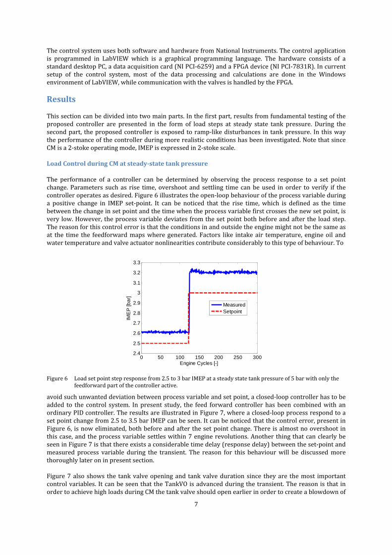
7
The control system uses both software and hardware from National Instruments. The control application is programmed in LabVIEW which is a graphical programming language. The hardware consists of a standard desktop PC, a data acquisition card (NI PCI‐6259) and a FPGA device (NI PCI‐7831R). In current setup of the control system, most of the data processing and calculations are done in the Windows environment of LabVIEW, while communication with the valves is handled by the FPGA.
Results
This section can be divided into two main parts. In the first part, results from fundamental testing of the proposed controller are presented in the form of load steps at steady state tank pressure. During the second part, the proposed controller is exposed to ramp‐like disturbances in tank pressure. In this way the performance of the controller during more realistic conditions has been investigated. Note that since CM is a 2‐stoke operating mode, IMEP is expressed in 2‐stoke scale.
Load Control during CM at steady‐state tank pressure
The performance of a controller can be determined by observing the process response to a set point change. Parameters such as rise time, overshoot and settling time can be used in order to verify if the controller operates as desired. Figure 6 illustrates the open‐loop behaviour of the process variable during a positive change in IMEP set‐point. It can be noticed that the rise time, which is defined as the time between the change in set point and the time when the process variable first crosses the new set point, is very low. However, the process variable deviates from the set point both before and after the load step. The reason for this control error is that the conditions in and outside the engine might not be the same as at the time the feedforward maps where generated. Factors like intake air temperature, engine oil and water temperature and valve actuator nonlinearities contribute considerably to this type of behaviour. To
Figure 6 Load set point step response from 2.5 to 3 bar IMEP at a steady state tank pressure of 5 bar with only the feedforward part of the controller active.
avoid such unwanted deviation between process variable and set point, a closed‐loop controller has to be added to the control system. In present study, the feed forward controller has been combined with an ordinary PID controller. The results are illustrated in Figure 7, where a closed‐loop process respond to a set point change from 2.5 to 3.5 bar IMEP can be seen. It can be noticed that the control error, present in Figure 6, is now eliminated, both before and after the set point change. There is almost no overshoot in this case, and the process variable settles within 7 engine revolutions. Another thing that can clearly be seen in Figure 7 is that there exists a considerable time delay (response delay) between the set‐point and measured process variable during the transient. The reason for this behaviour will be discussed more thoroughly later on in present section.
Figure 7 also shows the tank valve opening and tank valve duration since they are the most important control variables. It can be seen that the TankVO is advanced during the transient. The reason is that in order to achieve high loads during CM the tank valve should open earlier in order to create a blowdown of
0 50 100 150 200 250 3002.4
2.5
2.6
2.7
2.8
2.9
3
3.1
3.2
3.3
IME
P [b
ar]
Engine Cycles [-]
MeasuredSetpoint

8
compressed air from the tank into the cylinder and thus push the piston with negative force. The earlier the TankVO occurs the greater the difference in pressure level between the cylinder and the pressure tank will be with an increase in the negative force acting on the piston as a result.
Figure 7 Load step from 2.5 to 3.5 bar IMEP at a tank pressure of 5 bar (Closed loop process response to a set point change in CM IMEP from 2.5 bar to 4.5 bar at a steady‐state tank pressure of 5 bar)
Figure 8 Several load steps between 2.5 and 3.5 bar IMEP at a tank pressure of 5 bar
In Figure 8, the controller performance is tested by performing four consecutive set point changes, both positive and negative. There are some differences here compared to previous figure. For instance, the response delay ranges from 1 to 2 engine revolutions, compared to 3 engine revolutions in Figure 7. There is also a difference in settling time between the two figures, which has changed from 7 engine revolutions in Figure 7 to about 4 engine revolutions in Figure 8 , including the response delay. This means that if the response delay would be deducted, the settling time would be almost the same in both figures. It can be concluded from Figure 8 that both rise time and settling time are low without any visible overshoot and there seems to be no visible difference in controller performance between a positive and a negative set point change.
Figure 9 shows the process respond to a change in set‐point from 4 to 5 bar IMEP. The response delay is 1 engine revolution while the settling time is 3 engine revolutions. The reason why the settling time has decreased to 3 engine revolutions in comparison to 7 engine revolutions in Figure 7 is that the feedforward output is closer to the set point in this case and therefore the PID controller can do the final push towards the set‐point in a shorter time.
2.4
2.7
3
3.3
3.6
IME
P [b
ar]
MeasuredSetpoint
75
85
95
105
115
Ta
nkV
O [C
AD
BT
DC
]
150 200 250 30090
100
110
120
130
Ta
nkD
ur
[CA
D]
Engine Cycles [-]
2
2.5
3
3.5
4
IME
P [b
ar]
Measured Setpoint
75
85
95
105
115T
an
kVO
[CA
D B
TD
C]
50 100 150 200 250 300 350 400 45090
100
110
120
130
Ta
nkD
ur
[CA
D]
Engine Cycles [-]

9
Figure 9 Load step from 4 to 5 bar IMEP at a tank pressure of 8 bar
Figure 10 Several load steps between 4 and 5 bar IMEP at a tank pressure of 8 bar
In Figure 10, a series of both negative and positive set point changes between the same loads as in Figure 9 can be seen. Even though the response delay during all four set point changes is only 1 engine revolution, the settling time is about 7 engine revolutions. The reason is that the feedforward over predicts the output which leads to an overshoot in process response which the PID controller has to counteract.
In previous four figures, the amplitude of the set point change has been 1 bar IMEP. In next two figures, the amplitude of the set‐point changes will be 3 and 4 bar IMEP, respectively. In this way, the stability of the controller during large set point changes can be verified. Figure 11 shows process response during a positive set point change from 4 to 7 bar IMEP. Once again, the controller performs as expected, with low rise and settling time. In Figure 12, the process response to a negative set‐point change from 8 to 4 bar IMEP is shown. It can be seen that the controller has no problems controlling the output of the process during a relatively large set point change.
Figure 13 illustrates the process response during a set point change in the form of a staircase. The intention is to illustrate a more realistic increase from 4 to 7 bar IMEP during a braking event. In a real
3.9
4.2
4.5
4.8
5.1
IME
P [b
ar]
MeasuredSetpoint
80
86
92
98
104
Ta
nkV
O [C
AD
BT
DC
]
100 150 200 250 300104
110
116
122
128
Ta
nkD
ur
[CA
D]
Engine Cycles [-]
3.5
4
4.5
5
5.5
IME
P [b
ar]
Measured Setpoint
80
86
92
98
104
Ta
nkV
O [C
AD
BT
DC
]
100 200 300 400 500 600104
110
116
122
128
Ta
nkD
ur
[CA
D]
Engine Cycles [-]
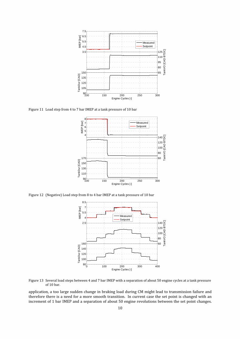
10
Figure 11 Load step from 4 to 7 bar IMEP at a tank pressure of 10 bar
Figure 12 (Negative) Load step from 8 to 4 bar IMEP at a tank pressure of 10 bar
Figure 13 Several load steps between 4 and 7 bar IMEP with a separation of about 50 engine cycles at a tank pressure of 10 bar.
application, a too large sudden change in braking load during CM might lead to transmission failure and therefore there is a need for a more smooth transition. In current case the set point is changed with an increment of 1 bar IMEP and a separation of about 50 engine revolutions between the set point changes.
3.5
4.5
5.5
6.5
7.5
IME
P [b
ar]
MeasuredSetpoint
65
80
95
110
125
Ta
nkV
O [C
AD
BT
DC
]
100 150 200 250 30090
105
120
135
150
Ta
nkD
ur
[CA
D]
Engine Cycles [-]
4
5
6
7
8
IME
P [b
ar]
MeasuredSetpoint
60
80
100
120
140
Ta
nkV
O [C
AD
BT
DC
]
100 150 200 250 30090
110
130
150
170
Ta
nkD
ur
[CA
D]
Engine Cycles [-]
2.5
4
5.5
7
8.5
IME
P [b
ar]
MeasuredSetpoint
60
80
100
120
140
Ta
nkV
O [C
AD
BT
DC
]
0 100 200 300 40080
100
120
140
160
Ta
nkD
ur
[CA
D]
Engine Cycles [-]

11
Once again the controller has no problems controlling the process response even though the time duration between changes in set point has decreased.
Figure 14 illustrates the difference between open‐loop load control (a) and closed‐loop load control (b) during steady state operation, i.e. with constant tank pressure. During open‐loop control it can be noticed that the control error increases throughout the experiment, again indicating the lack of adaptation to changes in for instance intake temperature, engine oil and water temperature when only a feedforward controller is used. During closed‐loop control, the process variable follows the set‐point quite well. However there are some oscillations present, which can clearly be seen in the control error part of Figure 14a. The reason for this behaviour is nonlinearities in the valve controlling the tank pressure [13]. The valve suffers from backlash which introduces a deadband within which the valve doesn’t respond to input signals. While the valve is in its deadband, the controller increases the control signal since the process variable remains unchanged and as soon as the valve comes out of its deadband, the controller output has grown too large which leads to excessive valve movement with an overshoot in process variable response as a result.
(a)
(b)
Figure 14 IMEP and the control error during steady state operation with only a feedforward controller (a) and with both PID and feedforward controllers (b).
Earlier in the present section it was established that there exists a response delay between the set point and the process variable during a transient. Figure 15, illustrates the response delay when the set point changes from 4 to 7 bar IMEP. The response delay is, in this particular case, 2 engine revolutions. The rise time of the process respond, not including the response delay, is also 2 engine revolutions. During the third revolution the process is mostly controlled by the feedforward controller and it takes an additional revolution for the PID controller to reach the set point the first time. This means that the total time it takes the controller to reach the desired set point is doubled compared to a system that would react instantly to a set point change.
3.8
3.9
4
4.1
4.2
IME
P [b
ar]
Setpoint Measured
0 50 100 150 200 250 300-1.5
0
1.5
Err
or
[%]
Engine Cycles [-]
3.8
3.9
4
4.1
4.2
IME
P [b
ar]
Setpoint Measured
0 50 100 150 200 250 300-1.5
0
1.5
Err
or
[%]
Engine Cycles [-]

12
Figure 15 A close‐up of a load step from 4 to 7 bar at a tank pressure of 10 bar illustrating the response delay between set point and process variable during a transient.
Figure 16 Histogram showing the distribution of the system response delay, here defined as the time duration between a change in set point and moment the control program outputs an updated control signal, i.e. the time delay due to communication with actuators is not included. Engine speed is 600 rpm.
The question to be answered is why these response delays occur. In Figure 16, the response delays from 135 consecutive set point changes are visualized in the form of a histogram. It can be noticed that the spread is quite large. However there are two areas on the x‐axis where a certain response delay occurs more frequently, in this case at a response delay of about 160 and 220 milliseconds, respectively. At an engine speed of 600 rpm this corresponds to a response delay of 2 and 3 engine revolutions, respectively. One reason for this occurrence is internal communication between different parts of the control program. The LabVIEW scheduler manages the timing and priorities of different parts of the application, and determines when each function should be executed. Since the execution is sequential, only one part of the application can execute at a time. This means that all other functions have to wait for their turn, and in worst case a deadline will be missed with an increase in response delay as a result. Another reason for the response delay occurrence is that the control program is not put on a dedicated real‐time PC. Instead a PC with Windows as operative system (OS) has been used which means that the control program also has to compete with other processes present in the Windows OS for available execution time which creates extra jitter in the control program execution. This problem can be avoided by moving the control application to a PC with a real‐time operative system (RTOS). In this way the CPU of the PC would only be dedicated to the control program. This kind of setup has been used by Zander et al. [14] for in‐cycle combustion control with promising results. Another possible solution with potential in decreasing the response delay is to put the load control loop directly on the FPGA. Since the FPGA allows real parallel execution at a speed of up to 40 MHz, the response delay could be decreased to a minimum.
154 156 158 160 162 164 166 1683.5
4
4.5
5
5.5
6
6.5
7
7.5
IME
P [b
ar]
Engine Cycles [-]
MeasuredSetpoint
100 150 200 2500
5
10
15
20
25
30
35
Fre
qu
en
cy [-
]
Response delay [ms]

13
Load control during CM at transient tank pressure
In previous section, the performance of the suggested controller has been investigated considering its behavior to set point changes during steady state tank pressure. However, in a real application the tank pressure will increase during a brake event. Therefore, the ability of the controller to reject disturbances has been tested. In current case, the disturbance is introduced as a ramp‐like increase in tank pressure. Figure 17 shows how the controller reacts to a disturbance in tank pressure. It can be noticed that there exists a bump in the process variable response immediately after the disturbance is introduced. However, the controller manages to reject the disturbance eventually. The maximum control error observed is less than 2% which corresponds to less than 0.1 bar of IMEP.
In Figure 17, the goal was to keep the process variable, i.e. the load, at a constant level. However, during a brake event the brake force demand will most likely vary and thus the CM load demand will also vary. Therefore, in Figure 18 a sequence of set point changes have been introduced in addition to the disturbance in tank pressure. Once again, the controller manages to maintain the process variable at the desired set point even though there is a disturbance in tank pressure indicating its suitability for real driving conditions. The maximum control error is again less than 2%.
Figure 17 A ramp‐like change in tank pressure and its effect on the control of IMEP. The vertical solid line denotes the start of change in tank pressure.
3
3.25
3.5
3.75
4
IME
P [b
ar]
MeasuredSetpoint
4
6
8
10
12
Ta
nk
Pre
ssu
re [b
ar]
40
55
70
85
100
Ta
nkV
O [C
AD
BT
DC
]
0 200 400 600 80080
90
100
110
120
Ta
nkD
ur
[CA
D]
Engine Cycles [-]
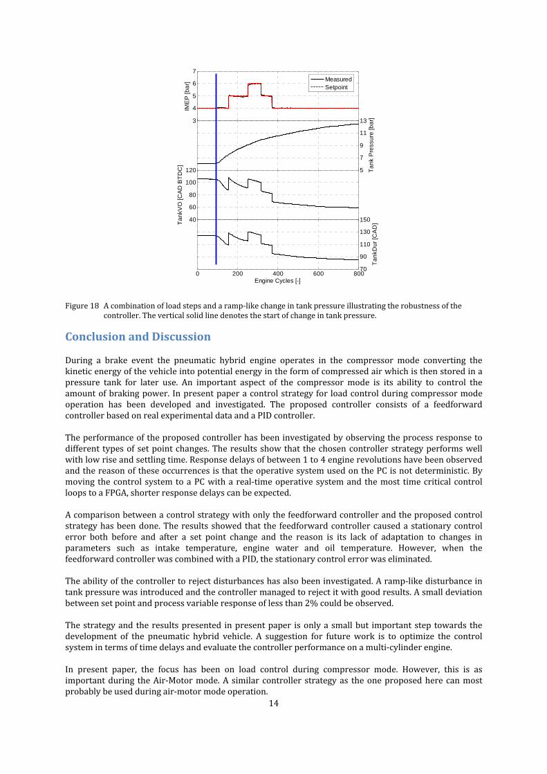
14
Figure 18 A combination of load steps and a ramp‐like change in tank pressure illustrating the robustness of the controller. The vertical solid line denotes the start of change in tank pressure.
Conclusion and Discussion
During a brake event the pneumatic hybrid engine operates in the compressor mode converting the kinetic energy of the vehicle into potential energy in the form of compressed air which is then stored in a pressure tank for later use. An important aspect of the compressor mode is its ability to control the amount of braking power. In present paper a control strategy for load control during compressor mode operation has been developed and investigated. The proposed controller consists of a feedforward controller based on real experimental data and a PID controller.
The performance of the proposed controller has been investigated by observing the process response to different types of set point changes. The results show that the chosen controller strategy performs well with low rise and settling time. Response delays of between 1 to 4 engine revolutions have been observed and the reason of these occurrences is that the operative system used on the PC is not deterministic. By moving the control system to a PC with a real‐time operative system and the most time critical control loops to a FPGA, shorter response delays can be expected.
A comparison between a control strategy with only the feedforward controller and the proposed control strategy has been done. The results showed that the feedforward controller caused a stationary control error both before and after a set point change and the reason is its lack of adaptation to changes in parameters such as intake temperature, engine water and oil temperature. However, when the feedforward controller was combined with a PID, the stationary control error was eliminated.
The ability of the controller to reject disturbances has also been investigated. A ramp‐like disturbance in tank pressure was introduced and the controller managed to reject it with good results. A small deviation between set point and process variable response of less than 2% could be observed.
The strategy and the results presented in present paper is only a small but important step towards the development of the pneumatic hybrid vehicle. A suggestion for future work is to optimize the control system in terms of time delays and evaluate the controller performance on a multi‐cylinder engine.
In present paper, the focus has been on load control during compressor mode. However, this is as important during the Air‐Motor mode. A similar controller strategy as the one proposed here can most probably be used during air‐motor mode operation.
3
4
5
6
7
IME
P [b
ar]
MeasuredSetpoint
5
7
9
11
13
Ta
nk
Pre
ssu
re [b
ar]
40
60
80
100
120
Ta
nkV
O [C
AD
BT
DC
]
0 200 400 600 80070
90
110
130
150
Ta
nkD
ur
[CA
D]
Engine Cycles [-]

15
References
1. Buchwald, P., Christensen, H., Larsen, H. and Pedersen, P.S.: Improvement of City bus Fuel Economy Using a Hydraulic Hybrid Propulsion System —a Theoretical and Experimental Study. SAE Paper 790305, Warrendale, PA, USA, 1979.
2. A. Folkesson, C. Andersson, P. Alvfors, M. Alaküla and L. Overgaard, ” Real life testing of a Hybrid PEM Fuel Cell Bus”, Journal of Power Sources 118, pp 349–357, 2003
3. D. Cross and C. Brockbank, “Mechanical Hybrid System Comprising a Flywheel and CVT for Motorsport and Mainstream Automotive Applications”, SAE Paper 2009‐01‐1312, 2009
4. M. Schechter, “Regenerative Compression Braking – A Low Cost Alternative to Electric Hybrids”, SAE Technical Paper 2000‐01‐1025, 2000
5. C. Tai, T‐C. Tsao, M. Levin, G. Barta and M. Schechter, “Using Camless Valvetrain for Air Hybrid Optimization, “SAE Technical Paper 2003‐01‐0038, 2003
6. I. Vasile, P. Higelin, A. Charlet and Y. Chamaillard, “Downsized engine torque lag compensation by pneumatic hybridization, 13th International Conference on Fluid Flow Technologies, 2006
7. C. Dönitz, I. Vasile, C. Onder and L. Guzzella, “Realizing a Concept for High Efficiency and Excellent Drivability: The Downsized and Supercharged Hybrid Pneumatic Engine”, SAE Technical Paper 2009‐01‐1326, 2009
8. S. Trajkovic, P. Tunestål, B. Johansson, U. Carlson and A. Höglund, “Introductory Study of Variable Valve Actuation for Pneumatic Hybridization”, SAE Technical Paper 2007‐01‐0288, 2007
9. S. Trajkovic, P. Tunestål and B. Johansson, “Investigation of Different Valve Geometries and Valve Timing Strategies and their Effect on Regenerative Efficiency for a Pneumatic Hybrid with Variable Valve Actuation”, SAE Int. J. Fuels Lubr. 1(1):1206‐1223, 2008
10. S. Trajkovic, P. Tunestål and B. Johansson, “A Simulation Study Quantifying the Effects of Drive Cycle Characteristics on the Performance of a Pneumatic Hybrid Bus”, ASME Technical Paper ICEF2010‐35093, 2010
11. S. Trajkovic, A. Milosavljevic, P. Tunestål and B. Johansson, ”FPGA Controlled Pneumatic Variable Valve Actuation”, SAE Technical Paper 2006‐01‐0041, 2006
12. J. Ma, T. Stuecken, U. Carlson, A. Höglund and M. Hedman, ”Analysis and Modeling of an Electronically Controlled Pneumatic Hydraulic Valve for an Automotive Engine”, SAE Technical Paper 2006‐01‐0042
13. H.D Baumann, “Control Valve Primer: A User’s Guide”, 4th ed., North Carolina: ISA, 2009 14. C.G. Zander, O. Stenlås, P. Tunestål and B. Johansson ” In‐cycle Closed Loop Control of the Fuel
Injection on a 1‐Cylinder Heavy Duty CI‐Engine”, ASME Paper ICEF2010‐35100, 2010
Contact
Sasa Trajkovic, PhD Student, MSc M.E.
E‐mail: [email protected]
Nomenclature
AM: Air‐motor Mode
APAM: Air Power Assist Mode
ATDC: After Top Dead Centre
BDC: Bottom Dead Centre
BTDC: Before Top Dead Centre
CM: Compressor Mode

16
FPGA: Field Programmable Gate Array
ICE: Internal Combustion Engine
IMEP: Indicated Mean Effective Pressure
IVC: Inlet Valve Closing
IVO: Inlet Valve Opening
OS: Operative System
RTOS: Real Time Operating System
TankVC: Tank Valve Closing
TankVO: Tank Valve Opening
TDC: Top Dead Centre