Embed Size (px)
Citation preview
DOCTORAL THESIS
“Essays on Monetary Policy, Wage Bargaining andFiscal Policy”
Stefano GnocchiUniversitat Pompeu Fabra
Department of Economics and Business
Advisor: Jordi Galı
November, 2007

Corresponding Address:
Stefano Gnocchi
Universitat Autonoma de Barcelona
Department of Economics and Economic History
Edifici B, Campus UAB
08193 Bellaterra, Barcelona
Spain
Phone: 0034 93 581 4324
Email: [email protected]
i

Contents
Acknowledgements v
Introduction vi
1 Non-Atomistic Wage Setters and Monetary Policy in a New-KeynesianFramework 11.1 Introduction . . . . . . . . . . . . . . . . . . . . . . . . . . . . . . . . . 11.2 The Model . . . . . . . . . . . . . . . . . . . . . . . . . . . . . . . . . . 4
1.2.1 Households . . . . . . . . . . . . . . . . . . . . . . . . . . . . . 51.2.2 Firms . . . . . . . . . . . . . . . . . . . . . . . . . . . . . . . . 71.2.3 Unions . . . . . . . . . . . . . . . . . . . . . . . . . . . . . . . . 91.2.4 The Sticky Price Equilibrium . . . . . . . . . . . . . . . . . . . 121.2.5 The Pareto Optimum . . . . . . . . . . . . . . . . . . . . . . . . 121.2.6 The Steady State . . . . . . . . . . . . . . . . . . . . . . . . . . 131.2.7 The Dynamics . . . . . . . . . . . . . . . . . . . . . . . . . . . . 16
1.3 Conclusions . . . . . . . . . . . . . . . . . . . . . . . . . . . . . . . . . 17
2 Optimal Simple Monetary Policy Rules and Non-Atomistic Wage Set-ters 222.1 Introduction . . . . . . . . . . . . . . . . . . . . . . . . . . . . . . . . . 222.2 The Model: Sticky Prices, Unionized Labor Markets and Wage Mark-up
Shocks . . . . . . . . . . . . . . . . . . . . . . . . . . . . . . . . . . . . 242.3 The Policy Problem . . . . . . . . . . . . . . . . . . . . . . . . . . . . . 26
2.3.1 The Welfare Criterion . . . . . . . . . . . . . . . . . . . . . . . 272.3.2 Average Distortion, Inflation Stabilization and Welfare . . . . . 292.3.3 The Trade-Off: an Additional Dimension . . . . . . . . . . . . . 32
2.4 Optimal Simple Policy Rules . . . . . . . . . . . . . . . . . . . . . . . . 332.5 Conclusion . . . . . . . . . . . . . . . . . . . . . . . . . . . . . . . . . . 39
ii

3 Discretionary Fiscal Policy and Optimal Monetary Policy in a Cur-rency Area 543.1 Introduction . . . . . . . . . . . . . . . . . . . . . . . . . . . . . . . . . 543.2 Literature Review . . . . . . . . . . . . . . . . . . . . . . . . . . . . . . 563.3 The Private Sector Equilibrium . . . . . . . . . . . . . . . . . . . . . . 58
3.3.1 Households . . . . . . . . . . . . . . . . . . . . . . . . . . . . . 593.3.2 Firms . . . . . . . . . . . . . . . . . . . . . . . . . . . . . . . . 643.3.3 Government Expenditure . . . . . . . . . . . . . . . . . . . . . . 653.3.4 Market Clearing . . . . . . . . . . . . . . . . . . . . . . . . . . . 653.3.5 The Pareto Optimum . . . . . . . . . . . . . . . . . . . . . . . . 663.3.6 Equilibrium Dynamics . . . . . . . . . . . . . . . . . . . . . . . 66
3.4 The Policy Problem . . . . . . . . . . . . . . . . . . . . . . . . . . . . . 683.5 Perfect Coordination . . . . . . . . . . . . . . . . . . . . . . . . . . . . 693.6 Optimal Monetary Policy under Fiscal Discretion . . . . . . . . . . . . 72
3.6.1 Union-wide Equilibrium . . . . . . . . . . . . . . . . . . . . . . 733.6.2 Equilibrium in The Representative Country . . . . . . . . . . . 75
3.7 Impulse Responses and Second Moments . . . . . . . . . . . . . . . . . 763.7.1 The Currency Area . . . . . . . . . . . . . . . . . . . . . . . . . 763.7.2 The Representative Country . . . . . . . . . . . . . . . . . . . . 77
3.8 Welfare Analysis . . . . . . . . . . . . . . . . . . . . . . . . . . . . . . 793.9 Conclusion . . . . . . . . . . . . . . . . . . . . . . . . . . . . . . . . . . 80
A Addendum to Chapter 1 93A.1 Labor Demand Elasticity . . . . . . . . . . . . . . . . . . . . . . . . . . 93A.2 Simulation and Numerical Results . . . . . . . . . . . . . . . . . . . . . 95
B Addendum to Chapter 2 101B.1 Appendix: Derivation of equation (2.4) . . . . . . . . . . . . . . . . . . 101B.2 Timelessly Optimal Fluctuations . . . . . . . . . . . . . . . . . . . . . 104B.3 Evaluation of suboptimal rules . . . . . . . . . . . . . . . . . . . . . . . 110B.4 Appendix: Derivation of coefficients fπ,a, fπ,u, fx,a and fx,u . . . . . . . 112B.5 Appendix: Derivation of equation (2.15) . . . . . . . . . . . . . . . . . 113
C Addendum to Chapter 3 115C.1 Perfect Coordination . . . . . . . . . . . . . . . . . . . . . . . . . . . . 115C.2 The Discretionary Fiscal Policy Problem . . . . . . . . . . . . . . . . . 116
C.2.1 The Currency Area Problem . . . . . . . . . . . . . . . . . . . . 117C.2.2 The Representative Country Problem . . . . . . . . . . . . . . . 117
iii

C.3 The Monetary Policy Problem . . . . . . . . . . . . . . . . . . . . . . . 119
iv

Acknowledgements
I thank Jordi Galı for his excellent supervision, his great support and his encouragement
to always challenge myself in search of improvement.
I also thank everybody I had the opportunity to talk to in UPF, in particular people
who followed my research closely, Christian Haefke, Michael Reiter and Thijs van Rens.
A special thank to Alessia Campolmi, Francesco Caprioli, Harald Fadinger and Chiara
Forlati for being friends, not just colleagues, and always staying close to me during
these years.
Part of my research have been developed while visiting the Econometric Modelling
Division at the European Central Bank. I enjoyed and benefitted from conversation
with Michele Lenza, Julian Morgan, Klaus Adam, Giacomo Carboni, Andrea Carriero,
Ania Lipinska and Julia Lendvai.
A very special thank to my parents, for their love, support and dedication.
Barcelona, November 2007 Stefano Gnocchi
v

Introduction
General equilibrium models with monopolistic competition and nominal rigidities have
become a workhorse in the design of the optimal monetary and fiscal policy response to
shocks over the business cycle. This literature pays scant attention to the role of strate-
gic interaction among private agents and policy makers. We identify two interesting
economic problems that can hardly abstract from the issue: the monetary policy impli-
cations of unionized labor markets; the coordination problems arising when monetary
and fiscal policy do not necessarily coordinate or agree on the optimal stabilization
policy mix. Those questions are analyzed in the context of a New-Keynesian frame-
work.
The first chapter generalizes the baseline New-Keynesian model to allow for a union-
ized labor force, a distinctive feature of labor markets in most of OECD countries. The
presence of large wage setters affects the transmission channel of monetary policy. Big
unions internalize the effects of their wage policy on inflation, by anticipating that a
rise in the wage produces inflationary pressures and a consequent reduction of labor
demand through monetary policy tightening. Tougher inflation stabilization policies
punish wage increases with a harsher contraction of aggregate labor demand, giving
unions the incentive to restrain real wages. In this context, the central bank can raise
long-run employment by implementing more aggressive stabilization policies. Strate-
gic interaction creates a transmission mechanism of monetary policy acting via labor
supply, rather than aggregate demand. The effectiveness of this channel increases in
wage setting centralization, as bigger unions internalize to a greater extent the impact
of their wage policy on inflation. As a consequence, depending on the labor market
structure, policy makers have an additional reason to stabilize inflation, other than
the usual concerns about relative price dispersion. This fact may be important in that
it is likely to alter the policy trade-off in favor of more conservative policies. Such a
question is the object of Chapter 2.
vi

Chapter 2 designs optimal monetary policy rules in a New-Keynesian model fea-
turing the presence of non-atomistic unions. The central bank faces an additional
trade-off with respect to the one traditionally considered in the literature. In fact,
steady state efficiency can be enhanced only by increasing aggressiveness in stabilizing
inflation, or equivalently only by accepting a higher volatility of the output gap. The
more is centralized the wage bargaining process, the higher is the marginal gain of sta-
bilizing inflation in terms of steady state efficiency, as the effectiveness of the strategic
interaction channel increases in labor market concentration. Consequently, the optimal
monetary policy stance is tighter. It turns out that concentrated labor markets call
for more aggressive stabilization policies. Finally, it is computed the cost of deviat-
ing from optimal policy. Such a cost is measured as the fraction of consumption that
agents are willing to give up to be indifferent between the optimal policy and a given
alternative regime. The welfare cost is decomposed in order to disentangle steady state
and stabilization effects of policy. The welfare analysis shows that most of the cost
can be accounted for by the steady state component. The result confirms the intuition
that in the presence of concentrated labor markets it is optimal to tighten monetary
policy, in order to exploit strategic interaction so as to increase long-run employment.
Chapter 3 evaluates the effects of fiscal discretion in a currency area, where a com-
mon and independent monetary authority commits to optimally set the union-wide
nominal interest rate. National governments implement fiscal policy by choosing gov-
ernment expenditure without coordinating with the central bank. The assumption of
fiscal policy coordination across countries is retained in order to evaluate the costs
exclusively due to discretion, leaving aside the free-riding problems stemming from
non-cooperation. In such a context, nominal rigidities potentially generate a stabi-
lization role for fiscal policy, in addition to the one of ensuring efficient provision of
public goods. However, it is showed that, under discretion, aggregate fiscal policy
stance is inefficiently loose and the volatility of government expenditure is higher than
vii

optimal. As an implication, the optimal monetary policy rule involves the targeting
of union-wide fiscal stance, on top of inflation and output gap. The result questions
the welfare enhancing role of government expenditure, as the proper instrument for
stabilizing asymmetric shocks. In fact, discretion entails significant welfare costs, the
magnitude depending on the stochastic properties of the shocks and, for plausible pa-
rameter values, it is not optimal to use fiscal policy as a stabilization tool.
viii

Chapter 1
Non-Atomistic Wage Setters andMonetary Policy in aNew-Keynesian Framework
1.1 Introduction
New-Keynesian (NK) models have been extensively used in recent years to analyze the
impact of monetary policy on business cycle fluctuations and to provide guidelines in
the design of optimal monetary policy rules.
NK literature commonly disregards potential strategic interaction between policy
makers and large wage setters, by assuming atomistic private agents. Yet, collective
wage bargaining is a distinctive feature of labor markets in most of OECD countries.
Figure 1.1 plots union density, measured as the fraction of workers affiliated to some
union, against bargaining coverage, defined as the fraction of workers covered by union-
negotiated terms and conditions of employment. Despite the historically low union
membership rates, a large fraction of wage contracts is negotiated in the context of
collective agreements: the average coverage level is twice as high as the density level (60
versus 34 percent). In continental Europe, at least two out of three workers are covered
by bargained wage setting with the exception of Switzerland and Eastern Europe. The
1

divergence between density and coverage is due to the widespread practice of extending
by law the collective contract to the non-unionized work force as well. Tables 1.1 and
1.2 show that several OECD countries feature highly centralized wage bargaining. In
fact, negotiations are delegated to few large unions whose decisions have a considerable
impact on the aggregate level of wages, which is in turn one of the main forces driving
the real cost of labor and, as a consequence, of inflation. In such an environment,
strategic interaction between wage setters and the monetary policymaker is an issue.
Although quite recent, the idea of studying how the presence of large wage setters
affects the monetary policy transmission channel is not new. Bratsiotis and Martin
(1999), Iversen and Soskice (2000) and Lippi (2002, 2003) among others1 show that, in
the presence of a unionized labor force, the systematic behavior of the central bank has
an impact on labor supply decisions and, as a consequence, on the long-run equilibrium
level of employment and production. These models are static and deterministic and
they hardly relate central bank’s targets to the microeconomic structure of the model
economy. As a consequence, they are silent on the optimal monetary policy response to
shocks over the cycle. Nevertheless, they identify a source of monetary non neutrality
that may well alter the traditional monetary policy results delivered by NK models.
Therefore, it may be a fruitful improvement upon the state of the art to merge these
two strands of the literature.
This chapter generalizes the baseline NK model to allow for a unionized labor
force. It is shown that, once the presence of large wage setters is taken into account,
an additional channel of transmission of monetary policy, other than the conventional
demand side channel, is created. The degree of wage setting centralization and the
aggressiveness of the central bank in stabilizing inflation jointly affect the equilibrium
1See also Cukierman and Lippi (1999) and Coricelli, Cukierman and Dalmazzo (2006). Holden(2005) took this literature a step forward by considering the effects of the monetary regime on wagesetters’ incentives to coordinate their decisions. Zanetti (2005) develops a NK model to study themonetary policy implications of unionized labor markets. His model however differs from the oneoutlined here, since atomistic unions are assumed.
2

level of real economic activity in the long-run. The classical neutrality result is not
challenged: a temporary shock to the policy instrument dies off in the long-run. A
change in the policy rule, however, has a permanent real effect since it alters the
steady state equilibrium level of employment. Two assumptions are key for the result:
wage setters have positive mass and they internalize the consequences of their actions.
Since wage setters are non-atomistic, they are able to influence the aggregate wage
index. In addition, if unions understand that firms set the price at a mark-up over the
marginal cost, they also realize that a variation in the aggregate wage index has an
impact on inflation, triggering the reaction of the central bank. Then, wage inflationary
pressures will induce the monetary authority to contract aggregate demand and, as a
consequence, aggregate labor demand. The higher central bank’s inflation aversion, the
stronger the response of the nominal interest rate and the more severe the contraction
of aggregate labor demand. Therefore, tougher inflation stabilization policies raise
the steady state level of employment by giving unions the incentive to restrain wages.
Because of strategic interaction, the central bank can push output towards Pareto
efficiency without creating inflation.
In this context, price stability is consistent with the elimination of any deviation
of real economic activity from Pareto efficiency and it is, as a consequence, the op-
timal policy. The outcome distinguishes the model outlined here from the standard
NK, where, without the proper fiscal policy, zero inflation under full commitment is
still optimal, but it can be reached only at the cost of a suboptimal production level.
Price stability as the optimal policy follows from the fact that price stickiness is the
only source of dynamic inefficiency. The introduction of other dynamic distortions
would introduce a tension between inflation and output gap stabilization and would
then undermine the policy implication. However, the main message would survive:
concentrated labor markets provide an additional reason to stabilize inflation fluctua-
tions other than the usual concerns about relative price dispersion. This fact may be
3

important in that it is likely to alter the trade-off traditionally considered in favor of
more conservative policies. Such a question is the object of Chapter 2.
The Chapter is organized as follows. Section 2 describes the model economy, the
main results and the policy implications. Section 3 concludes.
1.2 The Model
The model economy consists of a continuum of households and firms and a finite number
of unions. Households and firms are modelled as in the baseline NK model with goods
prices staggered a la Calvo (1983)2. The main differences with respect to the standard
framework are in the structure of the labor market. Households indeed delegate wage
setting decisions to unions and, for given wage, they are willing to supply whatever
quantity of labor is required to clear the markets.
The central bank sets the nominal interest rate, reacting to endogenous variations
in inflation according to the following policy rule
it = ρ+ γππt (1.1)
where it is the log of the nominal interest rate factor, ρ is the steady state level of it,
inflation is defined as πt = logPt − logPt−1 and γπ > 1.
It is assumed that the fiscal policy is responsible for offsetting the static distortions
arising because of imperfectly competitive goods markets, while, differently from the
baseline model, the inefficiency arising in labor markets is not corrected for. Lump-sum
transfers and taxes are available and they are free to adjust in order to balance the
government budget constraint at all times.
2For derivations of the baseline model I refer to Calvo (1983), Clarida, Galı and Gertler (1999),Galı (2003), Walsh (2003) and Woodford (2003)
4

1.2.1 Households
The economy is populated by a continuum of infinitely lived households indexed by i
on the unit interval [0,1], each of them consumes a continuum of differentiated goods
and supplies a differentiated labor type. Households have preferences defined over
consumption and hours worked described by the utility function3
E0
∞∑t=0
βt
[logCt,i −
L1+φt,i
1 + φ
](1.2)
where C is aggregate consumption, obtained aggregating in the Dixit-Stiglitz form the
quantities consumed of each variety f ∈ [0, 1]
Ct,i =
1∫0
Ct,i(f)θp−1
θp df
θp
θp−1
(1.3)
and the parameter θp > 1 is representing the elasticity of substitution among varieties.
Defining the aggregate price index4 as
Pt =
[∫ 1
0
Pt(f)1−θpdf
] 11−θp
(1.4)
optimal allocation of expenditure among varieties implies
C∗t,i(f) =
[Pt(f)
Pt
]−θp
Cti (1.5)
The budget constraint faced by households in each period is
Ct,i + δt,t+1Bt,i ≤ Bt−1,i +Wt,i
Pt
Lt,i + Tt,i +Divt,i (1.6)
δt,t+1 is the price vector of a state contingent asset paying one unit of consumption
in a particular state of nature in period t+1, Bt is the vector of the corresponding
3The analysis is restricted to the case of log utility. In this case not only the model is more tractable,but the policy analysis is particularly intuitive and transparent. However, it is possible to show thatall results derived here continue to hold in the more general case of a CRRA utility function.
4The price index has the property that the minimum cost of a consumption bundle Ct is PtCt
5

state contingent claims purchased by the household and Bt−1 the value of the claims
for the current realization of the state of nature.Wt,i
PtLt,i represents real labor income.
Finally, each consumer receives a share Divt,i of the aggregate profits and lump-sum
government transfers Tt,i. Households maximize their lifetime utility (1.2) subject to
the budget constraint (1.6) choosing state contingent paths of consumption and assets.
Optimal allocation of consumption over time implies the standard Euler equation
C−1t = Et[β(1 +Rt)C
−1t+1] = Et[β(1 + It)
Pt
Pt+1
C−1t+1] (1.7)
Rt, the risk-free real interest rate, is the rate of return of an asset that pays one unit
of consumption in every state of nature at time t+1 and the risk-free nominal interest
rate, It, is the rate of return of an asset that yields one unit of currency in every state
of nature at time t+1. Integrating (1.5) across households, total demand of variety f
is
C∗t (f) =
[Pt(f)
Pt
]−θp
Ct; Ct =
∫ 1
0
Ct,idi (1.8)
Let aggregate output Yt be defined by
Yt =
[∫ 1
0
Yt(f)θp−1
θp df
] θpθp−1
(1.9)
then the clearing of all goods markets
Yt,f = Ct,f (1.10)
implies
Yt = Ct (1.11)
Combining the Euler equation with the monetary policy rule, after imposing (1.11),
yields
Yt = Π−γπt
[Et
Π−1
t+1Y−1t+1
]−1(1.12)
where Πt is the gross inflation rate, defined as
Πt ≡Pt
Pt−1
(1.13)
6

Equation (1.12) fully describes the aggregate demand block of the model: it relates
aggregate output demand to inflation, conditionally on expectations about future vari-
ables. Note that the reaction of output to inflation depends on central bank’s aggres-
siveness in stabilizing inflation.
1.2.2 Firms
Consider a continuum of monopolistically competitive firms, indexed by f on the in-
terval [0, 1], each producing a differentiated good using a continuum of labor types
according to the following constant return to scale technology
Yt(f) = AtLt,f (1.14)
Productivity (TFP), denoted by At, follows an autoregressive process represented by
logAt+1 = ρalogAt + εt+1,a (1.15)
where εt is white noise with standard deviation σε,a. The effective labor input is ob-
tained aggregating in the Dixit-Stiglitz form the quantities hired of each differentiated
labor type
Lt,f =
[∫ 1
0
Lt,f (i)θw−1
θw di
] θwθw−1
The parameter θw > 1 is representing the elasticity of substitution among labor types.
Firms do not have market power in the labor market, then they take wages as given.
Defining the aggregate wage5 as
Wt =
[∫ 1
0
Wt(i)1−θwdi
] 11−θw
(1.16)
5As for the price index, aggregate wage has the property that the minimum cost of a unit ofcomposite labor input Lt is WtLt
7

cost minimization implies
L∗t,f (i) =
[Wt(i)
Wt
]−θw
Lt,f (1.17)
Firms set the price in order to maximize profits, subject to the constraint that demand
must be satisfied at the posted price, according to equation (1.8). Prices are set in
staggered contracts with random duration as in Calvo (1983): in any period each firm
faces a constant probability 1− α to reoptimize and charge a new price. A subsidy is
used by the fiscal authority to undo the steady state distortion induced by firms’ market
power in the goods markets. The definition of the price index and profit maximization
imply [1− αΠ
θp−1t
1− α
] 11−θp
=Et
∑∞j=0(αβ)jMCt+jΠ
θp
t,t+j
Et
∑∞j=0(αβ)jΠ
θp−1t,t+j
(1.18)
where Πt,t+j ≡ Pt+j
Ptand the real marginal cost is identical across firms and equal to
MCt =Wt
PtAt
(1.19)
Integrating (1.17) across firms yields total demand of labor faced by household i
L∗t (i) =
[Wt(i)
Wt
]−θw
Lt; Lt =
∫ 1
0
Lt,fdf (1.20)
It is convenient to rewrite (1.18) in the form
1− αΠθp−1t
1− α=
(Kt
Ft
)1−θp
(1.21)
defining K and F
Kt ≡ Et
∞∑j=0
(αβ)jMCt+jΠθp
t,t+j (1.22)
Ft ≡ Et
∞∑j=0
(αβ)jΠθp−1t,t+j (1.23)
8

Note that (1.22) and (1.23) can be expressed recursively as
Kt = MCt + αβEt
(Πt+1)
θpKt+1
(1.24)
Ft = 1 + αβEt
(Πt+1)
θp−1Ft+1
(1.25)
Equation (1.21) fully describes the aggregate supply block of the model: it relates
aggregate output supply to inflation, conditionally on expectations about future vari-
ables.
Finally, it can be easily shown that the aggregate production function is given by
Yt∆t = AtLt (1.26)
where ∆t6 is defined as
∆t =
∫ 1
0
Yt(f)
Yt
df (1.27)
and represents a measure of relative price dispersion, evolving according to the law
∆t = (1− α)
(1− αΠ
θp−1t
1− α
) θpθp−1
+ αΠθp
t ∆t−1 (1.28)
1.2.3 Unions
The economy is populated by a finite number of unions indexed by j, where j ∈1, ..., n, n ≥ 2. All workers are unionized and they split equally among unions so
that each union has mass n−1. The mass can be interpreted as the degree of wage
setting centralization (CWS) as well as unions’ ability to internalize the consequences
of their actions. As a matter of fact, the higher is the number of unions the lower
6It can be proved that log(∆) is a function of the cross sectional variance of relative prices and itis of second order.
9
is their mass and then the lower the impact of union’s j wage policy on aggregate
variables.
It is assumed that wages are fully flexible and any possibility of pre-commitment
to future wage policies is ruled out. Each union j sets the real wage on behalf of
her members to maximize their lifetime utility function (1.2) subject to the budget
constraint7 (1.6) and labor demand (1.20) for all members i ∈ j. Unions set wages
simultaneously and each of them takes other unions’ real wages as given.
The assumption that wage setters have positive mass is key for the outcome of the
model. Since unions are non-atomistic, they internalize the impact of their wage policy
on the aggregate wage. Then they also realize that an increase in union’s j wage creates
inflationary pressures via the price setting rule of firms, inducing the central bank to
contract aggregate demand, and then aggregate labor demand. Formally, the aggregate
wage index (1.16), aggregate demand (1.12), the production function (1.26) and the
short run aggregate supply (1.21) are internalized on top of the budget constraint (1.6)
and labor demand (1.20). It follows that aggregate labor demand is a function ofWj,t
Pt
through the monetary policy rule. The elasticity of aggregate labor demand to changes
in the wage is8
ΣL = γπ(1− α)(1− αβ)
α(1.29)
implying the following elasticity of labor demand perceived by the j-th union for each
of her members
η = θw(1− 1
n) +
1
nΣL (1.30)
This is a weighted average of the elasticity of substitution among labor types and the
7Fiscal policy and dividends are taken as given, as it is usually assumed in the literature. See Lippi(2002, 2003)
8For the derivation of ΣL see Appendix A. Note that ΣL is not constant over time. However, asit is shown in the appendix, for empirically relevant values of the parameters and for the calibrationsconsidered below, elasticity fluctuations do not generate quantitatively significant variation out of thesteady state at a first-order accuracy. Then it is assumed in the rest of the chapter that elasticity isconstantly equal to its steady state value.
10
elasticity of aggregate labor demand, which is in turn an increasing function of γπ. This
is because the more is restrictive the policy stance, the harsher will be the contraction of
aggregate demand as a reaction to inflation variability, with the consequence of making
labor demand more sensitive to a variation in the wage. The effect is increasing in the
mass of the union as larger unions internalize more the impact of their wage policy on
aggregate variables. Note that price stickiness enters negatively through the elasticity
of aggregate labor demand. Indeed, when price stickiness raises, the fraction of firms
re-optimizing in each period is lower. Therefore, also the impact of a change in the
real wage on inflation, and then on aggregate output through central bank’s reaction,
has to be lower.
The solution to unions’ problem implies the following relation
Wt
Pt
=η
η − 1Lφ
tCt (1.31)
Index j has been dropped because of symmetry. The first order condition for unions
has the same form as in the standard case with atomistic wage setters. The real wage in
fact is set at a mark-up over the marginal rate of substitution. However, the mark-up
depends not only on the elasticity of substitution among labor types, but also on the
number of unions and on central bank’s aggressiveness in stabilizing inflation. Tough
inflation stabilization policies discourage wage pressures by punishing a wage increase
with a contraction of aggregate demand. Note finally that unions have been modelled
in such a way that the case of non-atomistic wage setters nests the two limiting cases
of monopolistically competitive and perfectly competitive labor markets. When the
number of unions tends to infinity, the wage mark-up becomes θw
θw−1. Alternatively, if
the elasticity of substitution between labor types tends to infinity, the wage collapses
to the competitive level.
11

1.2.4 The Sticky Price Equilibrium
Given ∆−1, the exogenous stochastic process At and a value for the policy parame-
ter γπ, the rational expectation equilibrium for the sticky price economy is a process
Yt,Πt, Ft, Kt,∆t∞t=0 satisfying the following system of equations
Y −1t = Πγπ
t EtΠ−1t+1Y
−1t+1
1− αΠθp−1t
1− α=
(Kt
Ft
)1−θp
Kt =η
η − 1
(Yt
At
)1+φ
∆φt + αβEt
(Πt+1)
θpKt+1
Ft = 1 + αβEt
(Πt+1)
θp−1Ft+1
∆t = (1− α)
(1− αΠ
θp−1t
1− α
) θpθp−1
+ αΠθp
t ∆t−1
η = θw(1− 1
n) +
1
nγπ
(1− α)(1− αβ)
α
which can be easily obtained using equations (1.11), (1.12), (1.19), (1.21), (1.24), (1.25),
(1.26), (1.28), (1.30) and (1.31).
1.2.5 The Pareto Optimum
For the subsequent analysis it is useful to derive the Pareto efficient level of output,
consumption and labor. Pareto efficiency requires that the marginal rate of substi-
tution between consumption and leisure equalizes the corresponding marginal rate of
transformation
12

At = LφtCt (1.32)
The goods market clearing condition (1.11) and the production function (1.26), can be
used to get the Pareto efficient values of output
Y ∗t = At (1.33)
and employment
L∗t = 1 (1.34)
Hence, at the non-stochastic steady state
Y ∗ = C∗ = L∗ = 1
1.2.6 The Steady State
The non-stochastic steady state of the model is derived setting the shocks to their mean
value. It is straightforward to prove that the steady state level of the gross inflation
rate and price dispersion are equal to one, using aggregate demand and the law of
motion for price dispersion. Moreover, from the short run aggregate supply and the
definition of the auxiliary variables Kt and Ft, we can obtain the steady state value of
output, employment and consumption
Y = L = C =
[1− 1
η
] 11+φ
(1.35)
The result can be easily compared with the two benchmark cases usually studied in
the literature, monopolistic competition and perfectly competitive labor markets, that
can in turn be seen as particular cases of the non-atomistic wage setters framework.
Letting the number of unions tend to infinity, employment, consumption and output
are back to the monopolistic competition levels
limn→∞
L = limn→∞
[1− 1
η
] 11+φ
=
[θw − 1
θw
] 11+φ
(1.36)
13

When indeed there are infinitely many unions, their mass tends to zero and they do
not internalize the effect of their actions on the aggregate variables. As a consequence,
the strategic interaction channel is shut down and the degree of Pareto inefficiency
depends only on the degree of substitutability among labor types in the production
process.
The perfect competition result arises instead when perfect substitutability among
labor types is assumed
limθw→∞
L = limθw→∞
[1− 1
η
] 11+φ
= 1 (1.37)
as labor demand becomes perfectly elastic.
Some conclusions can be drawn looking at the steady state level of employment
(1.35).
First, recall from (1.34) that the efficient level of employment is L∗t = 1. Hence,
the steady state is not Pareto efficient: imperfect substitutability of labor types and
the presence of unions drive a wedge between the marginal productivity of labor and
the marginal rate of substitution, determining a suboptimal employment equilibrium
level. As market power on the goods markets is offset by fiscal policy, the steady state
distortion is coming exclusively from the labor market side.
Second, the steady state is not independent of the monetary policy rule. This is
because the central bank is able to induce wage restraint by implementing tougher sta-
bilization policies. Then the steady state level of employment, output and consumption
are increasing functions of the coefficient entering the Taylor rule. The outcome of the
model does not challenge the conventional neutrality result: a transitory shock to the
nominal interest rate dies off in the long run and leaves the steady state unaffected.
The way in which the central bank systematically behaves, however, has an impact on
real economic activity.
Moreover, the labor market structure interacts with monetary policy in determining
14

the long-run equilibrium values of the real variables. In fact, the way in which a change
in the degree of wage setting centralization affects equilibrium depends on the monetary
policy stance: a less unionized labor market enhances welfare, provided that monetary
policy is not too aggressive in stabilizing inflation. To prove it, it is sufficient to look at
the elasticity of labor demand perceived by the j-th union (1.30). As it is a weighted
average between θw and ΣL, where the weights are respectively 1 − 1/n and 1/n, η
increases in n if and only if θw > ΣL. This is equivalent to say that η increases in n if
and only if
γπ ≤ γπ (1.38)
where
γπ ≡ θwα
(1− α)(1− αβ)(1.39)
As the steady state is in turn increasing in η, a decentralization of wage setting raises
long-run employment only when (1.38) is satisfied. This result is quite intuitive. The
presence of unions has two opposite effects: on one side the higher market power tends
to depress employment; on the other hand, the strategic interaction channel of mone-
tary policy tends to increase employment restraining real wage demands. The second
effect decreases with the number of unions, because unions with a lower mass internal-
ize less the consequences of their actions on aggregate variables. When the central bank
is aggressive, the wage restraint induced by monetary policy is very important and it
may be excessively costly to reduce the degree of wage setting centralization. When
(1.38) is satisfied, the argument is reversed and the lower is the mass of the unions, the
higher is welfare. For a sensible calibration of parameters, the threshold value of γπ is
much higher than the one empirically observed9. Then, for empirically plausible values
of parameters, a decentralization in the wage bargaining process is welfare enhancing.
This seems to be in contrast with some contributions pointing towards a hump-shaped
9For the calibration considered below and displayed in Table 3 the threshold value is equal to128.1553
15

relation between centralization of wage setting and employment10. This is because the
model is well defined only for n ≥ 2. A single encompassing union would act as a
planner and would behave so as to attain Pareto efficiency, independently of monetary
policy.
Finally, in the case of γπ →∞, efficiency is restored
limγπ→∞
L = limγπ→∞
[1− 1
η
] 11+φ
= 1 (1.40)
This case is known in the literature as strict inflation targeting. When the coefficient
entering the Taylor rule tends to infinity, inflation is on target not only on average, but
also period by period. Since the target inflation rate implied by the specified Taylor rule
is zero, strict inflation targeting allows the central bank to achieve price stability also
outside the steady state. The model predicts that strict inflation targeting implements
Pareto efficiency in the long run, through the strategic interaction channel. This result
introduces an additional reason to penalize deviations from price stability.
1.2.7 The Dynamics
Log-linearizing the model around the non-stochastic steady state allows to fully char-
acterize the equilibrium dynamics at a first order accuracy by
xt = Etxt+1 − (it − Etπt+1 − r∗t ) (1.41)
πt = βEtπt+1 +(1− α)(1− αβ)
α(1 + φ)xt (1.42)
(1.41) and (1.42) are respectively the conventional IS equation and the New-Keynesian
Phillips curve (NKPC) and r∗t is an exogenous disturbance defined as
r∗t = −(1− ρa)at + ρ
10For instance, this is the case made by Calmfors and Driffill (1988). However, the empirical andthe literature are far from having reached a consensus in this respect. For a survey of the issue, seeCalmfors (2001).
16

Note that the output gap
xt ≡ yt − y∗t (1.43)
refers to output deviations from Pareto efficiency rather than from the flexible price
equilibrium. In fact, the flexible price equilibrium does not need to be efficient, as fiscal
policy is not assumed to offset the static distortion arising from imperfectly competitive
labor markets. Therefore, it is more insightful to relate inflationary pressures to a
welfare relevant variable such as the gap between actual and efficient output.
From the Phillips curve, it is immediate to see that strict inflation targeting allows
to fully stabilize the output gap. The steady state value of the gap depends on the
monetary policy stance and, as it has been previously showed, it is zero under a strict
inflation targeting policy. Hence, price stability is consistent with the elimination of any
deviation of real economic activity from Pareto efficiency and it is, as a consequence, the
optimal policy. This is the outcome of strategic interaction: the central bank affects the
equilibrium level of output not only through aggregate demand, but also through labor
supply. Then, it is possible to push the economy towards Pareto efficiency without
creating inflation. This result distinguishes the model outlined here from the standard
NK, where, without the proper fiscal policy, zero inflation under full commitment is
still optimal, but can be reached only at the cost of a suboptimal production level.
1.3 Conclusions
This Chapter builds a model where the presence of large wage setters creates a new
monetary policy transmission channel. Two main differences with respect to the base-
line model should be highlighted.
First, the policy rule has a permanent effect on real economic activity, while in the
standard framework changes in the policy rule do not have any effect on the steady
state value of real variables.
17
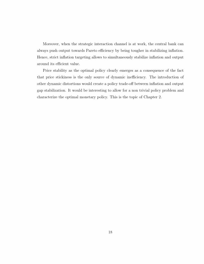
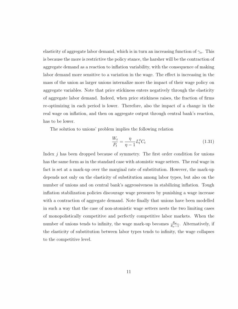
Moreover, when the strategic interaction channel is at work, the central bank can
always push output towards Pareto efficiency by being tougher in stabilizing inflation.
Hence, strict inflation targeting allows to simultaneously stabilize inflation and output
around its efficient value.
Price stability as the optimal policy clearly emerges as a consequence of the fact
that price stickiness is the only source of dynamic inefficiency. The introduction of
other dynamic distortions would create a policy trade-off between inflation and output
gap stabilization. It would be interesting to allow for a non trivial policy problem and
characterize the optimal monetary policy. This is the topic of Chapter 2.
18

Figure 1.1: Union density versus union coverage in OECD countries, 2000.Source: OECD Employment Outlook 2004. Percentage of wage earners.
Union Density vs. Coverage, 2000source: OECD 2004 Employment Oultook
Australia
Austria
Belgium
Canada
Czech Republic
Denmark
FinlandFrance
Germany
Hungary
Italy
Japan
Korea
Luxembourg
Netherlands
New Zealand
Norway
Poland
Portugal
Slovak Republic
Spain
Sweden
Switzerland
United Kingdom
United States
0,0
10,0
20,0
30,0
40,0
50,0
60,0
70,0
80,0
90,0
100,0
0,0 10,0 20,0 30,0 40,0 50,0 60,0 70,0 80,0 90,0 100,0
Union Density (%)
Co
ver
age
(%)
19
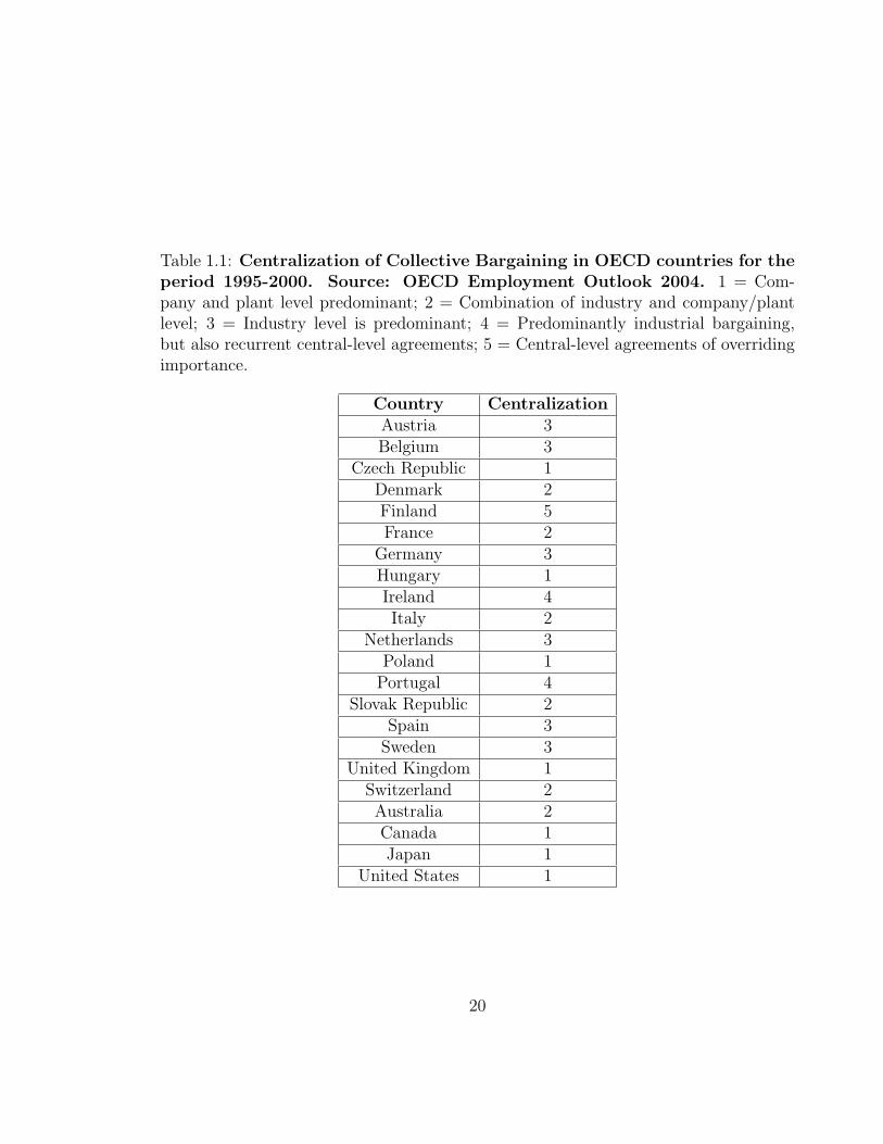
Table 1.1: Centralization of Collective Bargaining in OECD countries for theperiod 1995-2000. Source: OECD Employment Outlook 2004. 1 = Com-pany and plant level predominant; 2 = Combination of industry and company/plantlevel; 3 = Industry level is predominant; 4 = Predominantly industrial bargaining,but also recurrent central-level agreements; 5 = Central-level agreements of overridingimportance.
Country CentralizationAustria 3Belgium 3
Czech Republic 1Denmark 2Finland 5France 2
Germany 3Hungary 1Ireland 4Italy 2
Netherlands 3Poland 1
Portugal 4Slovak Republic 2
Spain 3Sweden 3
United Kingdom 1Switzerland 2Australia 2Canada 1Japan 1
United States 1
20
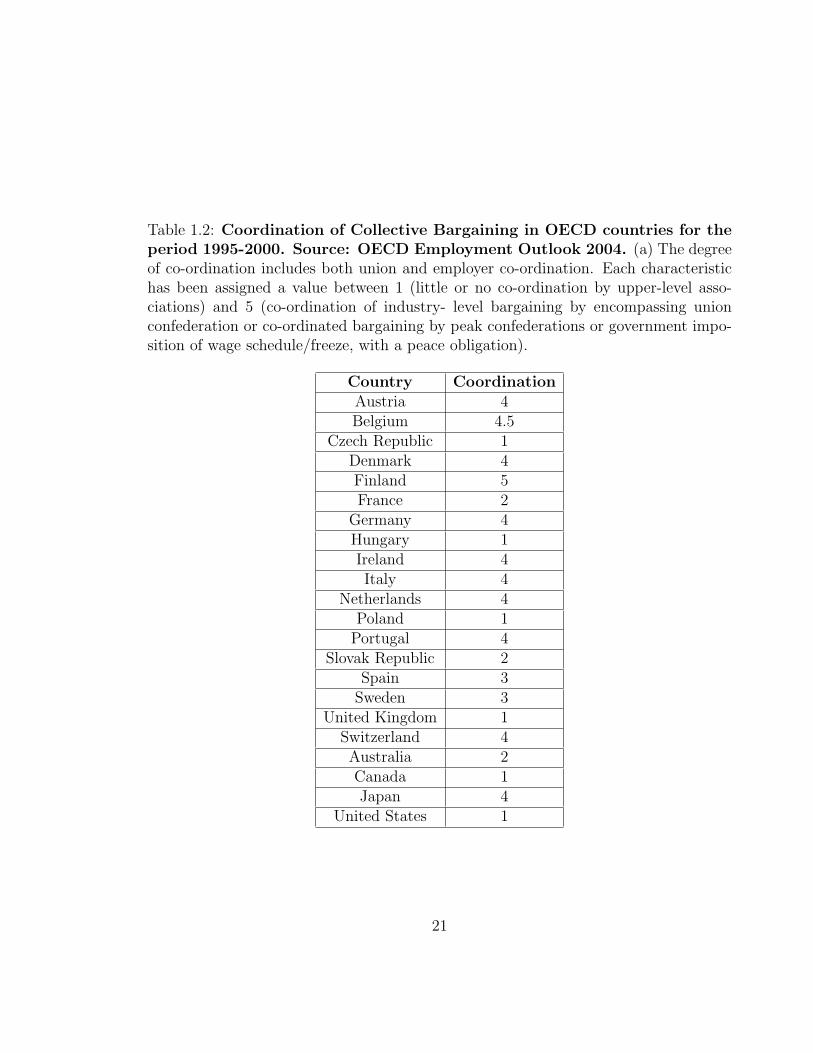
Table 1.2: Coordination of Collective Bargaining in OECD countries for theperiod 1995-2000. Source: OECD Employment Outlook 2004. (a) The degreeof co-ordination includes both union and employer co-ordination. Each characteristichas been assigned a value between 1 (little or no co-ordination by upper-level asso-ciations) and 5 (co-ordination of industry- level bargaining by encompassing unionconfederation or co-ordinated bargaining by peak confederations or government impo-sition of wage schedule/freeze, with a peace obligation).
Country CoordinationAustria 4Belgium 4.5
Czech Republic 1Denmark 4Finland 5France 2
Germany 4Hungary 1Ireland 4Italy 4
Netherlands 4Poland 1
Portugal 4Slovak Republic 2
Spain 3Sweden 3
United Kingdom 1Switzerland 4Australia 2Canada 1Japan 4
United States 1
21

Chapter 2
Optimal Simple Monetary PolicyRules and Non-Atomistic WageSetters
2.1 Introduction
Chapter 1 extends a baseline DSGE model with sticky prices to the case of a unionized
labor force. The goal of the present Chapter1 is to allow for a non trivial policy
trade-off in a NK model augmented with unions and to study how such a trade-off is
modified depending on the labor market structure, in order to characterize the optimal
monetary policy. As a first step the analysis is restricted to the case of simple rules,
while the case of the fully optimal policy is left to future research. The design of the
optimal policy rule is performed by using the methodology introduced by Rotemberg
and Woodford (1997) and further developed by Benigno and Woodford (2005). The
method resorts to a second order approximation to households’ lifetime utility as an
approximate welfare measure. Because of the long-run non-neutrality of the rule, the
welfare measure is decomposed in such a way to disentangle the steady state and the
stabilization effects of policy.
1The first version of the paper on which the chapter is based has been circulated as ECB WorkingPaper No.690, October 2006, http://ecb.int/pub/pdf/scpwps/ecbwp690.pdf
22
We show that the presence of large wage setters creates an additional dimension of
the policy trade-off with respect to the one traditionally considered by the literature.
This is because in a model with unions, being more aggressive in stabilizing inflation
allows to reduce steady state distortion by inducing wage restraint. But, as tougher
inflation stabilization policies amplify output gap volatility, the policy maker has to
trade-off steady state efficiency against dynamic efficiency. Two are the forces underly-
ing the policy dilemma: wage setting centralization and the volatility of the cost push
shock. Highly centralized labor markets are associated to high gains of aggressiveness
in terms of average distortion. In fact, larger unions internalize more the impact of
their wage policy on inflation, making more effective the strategic interaction channel
of monetary policy. On the other hand, the more volatile is the cost push shock, the
more costly is price stability in terms of gap fluctuations. This implies a high cost of
reducing average distortion.
The two forces interact resolving the policy trade-off and determining the following
optimal policy results.
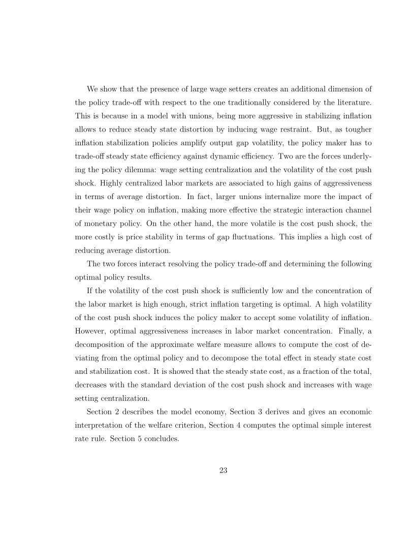
If the volatility of the cost push shock is sufficiently low and the concentration of
the labor market is high enough, strict inflation targeting is optimal. A high volatility
of the cost push shock induces the policy maker to accept some volatility of inflation.
However, optimal aggressiveness increases in labor market concentration. Finally, a
decomposition of the approximate welfare measure allows to compute the cost of de-
viating from the optimal policy and to decompose the total effect in steady state cost
and stabilization cost. It is showed that the steady state cost, as a fraction of the total,
decreases with the standard deviation of the cost push shock and increases with wage
setting centralization.
Section 2 describes the model economy, Section 3 derives and gives an economic
interpretation of the welfare criterion, Section 4 computes the optimal simple interest
rate rule. Section 5 concludes.
23

2.2 The Model: Sticky Prices, Unionized Labor
Markets and Wage Mark-up Shocks
Consider the same economy as in Chapter 1. The model outlined there shares with
the baseline NK model an unpleasant feature: the lack of a non-trivial policy trade-off,
which is perceived to be as an empirically relevant problem by any central banker. It is
needed to create a tension between inflation and output gap stabilization. Therefore,
it is assumed from now on that the wage mark-up is fluctuating exogenously around
its mean value2. The first order condition is modified accordingly to include a random
shockWt
Pt
= expµwt
η
η − 1Lφ
tCt (2.1)
µwt follows an autoregressive process represented by
µwt+1 = ρuµ
wt + εt+1,u (2.2)
where εt,u is white noise with standard deviation denoted by σε,u3.
Whenever the economy is hit by wage mark-up shocks, it is not feasible to attain the
Pareto efficient outcome by stabilizing inflation. In fact, complete inflation stabilization
replicates the flexible price equilibrium, which is not efficient because of stochastic
deviations of the real wage from the marginal rate of substitutions. As a consequence,
the central bank has to trade-off inflation fluctuations against output deviations from
Pareto efficiency.
2This can be seen as a shortcut to include other forms of nominal rigidities, such as wage stickiness.See also Clarida et al. (1999), Galı (2003) and Woodford (2003)
3As before ΣL is not constant over time. Again, you can show that, for empirically relevant valuesof the parameters and for the calibrations considered below, elasticity fluctuations do not generatequantitatively significant variation out of the steady state at a second-order accuracy. To this purposethe model has been approximated to second order and simulated using the method developed bySchmitt-Grohe and Uribe (2004b). Then it is assumed in the rest of the paper that elasticity isconstantly equal to its steady state value. This is inconsequential also for the results obtained in thewelfare analysis.
24

As the dynamics of the model is now driven by an additional shock, the sticky
price allocation can be redefined as it follows. Let xt = (Yt,Πt,∆t) and Xt = (Ft, Kt).
Given ∆−1, exogenous stochastic processes At and µwt and given a value for the policy
parameter γπ, the rational expectation equilibrium for the sticky price economy is a
process xt, Xt∞t=0 that satisfies the following system of equations
Y −1t = Πγπ
t EtΠ−1t+1Y
−1t+1
1− αΠθp−1t
1− α=
(Kt
Ft
)1−θp
Kt =η
η − 1expµw
t (Yt
At
)1+φ
∆φt + αβEt
(Πt+1)
θpKt+1
Ft = 1 + αβEt
(Πt+1)
θp−1Ft+1
∆t = (1− α)
(1− αΠ
θp−1t
1− α
) θpθp−1
+ αΠθp
t ∆t−1
η = θw(1− 1
n) +
1
nγπ
(1− α)(1− αβ)
α
While changing the dynamics, the presence of cost push shocks does not alter the
steady state of the economy. Hence, the analysis performed in Chapter 1 continues to
hold.
Before introducing the policy problem, it is convenient to define a measure of aver-
age distortion. A reasonable candidate is the wedge between marginal productivity and
the marginal rate of substitution. While the efficient steady state implies the following
marginal rate of substitution
mrs∗ = (L∗)φC = 1
25

at the actual steady state
mrs = LφC = 1− η−1
so that Φ ≡ η−1 can be defined as a measure of steady state inefficiency.
2.3 The Policy Problem
The previous section defines the private sector equilibrium when the central bank
credibly commits to a monetary policy rule. The policy problem faced by the central
bank can then be described as the choice of the coefficients entering the rule, taking
into account the reaction of the agents to the policy commitment.
I wish to find the optimal monetary policy rule within a class of simple and im-
plementable rules of the kind described by equation (1.1). A rule is said to be im-
plementable if it brings about a locally unique rational expectation equilibrium in a
neighborhood of the non-stochastic steady state, under the assumption of sufficiently
tightly bounded exogenous processes. An implementable rule is optimal, within the
particular family of policies taken into consideration, if it yields the highest value for
a suitably defined welfare criterion.
The definition of such a criterion and the analysis of its implications for the mon-
etary policy problem are the objects of the section. The issue is addressed using the
linear-quadratic approach introduced by Rotemberg and Woodford (1997) and further
developed by Benigno and Woodford (2005). Because of the long-run non-neutrality
of the rule, the welfare measure is decomposed in such a way to disentangle the steady
state and the stabilization effects of policy.
Optimality is judged from a timeless perspective. For a policy to be optimal in this
sense, it is sufficient to limit central bank’s ability to exploit the expectations already
in place at the time the commitment is chosen.
26

2.3.1 The Welfare Criterion
The conditional expectation of lifetime utility as of time zero is
U0 = E0
∞∑t=0
βt
[logCt −
L1+φt
1 + φ
](2.3)
It might seem natural to define the optimal policy rule at time zero as the one
that maximizes (2.3) subject to the constraints imposed by the behavior of the private
sector. However, the use of (2.3) leads to a time inconsistent selection of the rule.
This is because the optimal choice correctly takes into account the effects of policy
on future expectations, but not on the expectations formed prior to time zero. Past
expectations about current outcomes are in fact given at the time of policy selection. As
a consequence, should the policy be reconsidered at a later period, the new commitment
would not be a continuation of the original plan: the policy maker has the incentive
to fool the agents whenever she has the possibility of revising her commitments. To
overcome the time inconsistency problem, I closely follow Benigno and Woodford (2005)
who propose to penalize the rules exploiting the expectations already in place at the
time the commitment is chosen. According to their method the welfare criterion can
be defined in three steps. The intuition of the procedure is described below while I
refer to the appendix for the technical details.
First, one needs to characterize the unconstrained timelessly optimal policy. The
term unconstrained here refers to the fact that the optimal policy does not necessarily
need to be implemented by a simple policy rule of the kind described by equation
(1.1). Note also that, differently from the case studied by Benigno and Woodford
(2005), average distortion is controlled by the monetary authority.
Second, it is computed the gain of fooling the agents, that is the value of choosing
a policy that does not validate past expectations about current equilibrium outcomes.
This is equivalent to compute the gain of deviating from the timelessly optimal plan.
Finally, the welfare criterion is constructed by subtracting from U0 the gain of
27

fooling the agents, Ψ(µw,0), associated to the policy under scrutiny
U0 = U0 −Ψ(µw,0)
Since Ψ(µw,0) is a function of the whole history of cost push disturbances up to time
zero, it is computed the unconditional expected value of the modified welfare criterion,
integrating over all possible histories of shocks. A second order approximation to U0
yields the purely quadratic approximate welfare measure
W0 =U(Φ)
1− β− 1
2
Φ(1− Φ)
1 + φE
∞∑t=0
βt(µwt )2 +
−1
2
θp
λE
∞∑t=0
βt
[π2
t + (1 + φ)λ
θp
x2t
]− EΨ(µw,0) (2.4)
where λ = (1−α)(1−αβ)α
and U is the steady state level of utility. All variables are
expressed in log deviations from the non-stochastic steady state and the welfare relevant
output gap
xt ≡ yt − y∗t
is defined as the output deviation from a properly defined target
y∗t ≡ at −Φ
1 + φµw
t
The welfare criterion can be used not only to determine the rule that is optimal
within a given class, but also to compute the cost of deviating from the optimized
rule. Consider two policy regimes, R (reference) and A (alternative), respectively
characterized by the induced allocations (CRt , L
Rt ∞t=0) and (CA
t , LAt ∞t=0). Then the
associated welfare is
UR = U(CRt , L
R∞t=0) and UA = U(CAt , L
A∞t=0)
28

Let the cost of regime A be denoted by γ. I measure γ as the fraction of regime R’s
consumption that households would be willing to give up in order to be as well off as
under regime A. Formally it is implicitly defined by
U((1− γ)CRt , L
R∞t=0) = U(CAt , L
A∞t=0)
It can be easily shown that, given the functional form of the utility function
γ = 1− exp(1− β)(UA − UR) (2.5)
2.3.2 Average Distortion, Inflation Stabilization and Welfare
A well defined approximate welfare measure allows to analyze what are the objectives
of a benevolent central bank willing to choose the state-contingent path of the economic
variables preferred by the private sector. It turns out that, differently from a standard
NK framework, the evaluation of alternative policies cannot disregard possible effects
stemming from the policy rule non-neutrality due to the presence of unionized labor
markets.
In fact, the welfare function can be decomposed into two parts: a stabilization com-
ponent measuring the welfare effects of fluctuations around the non-stochastic steady
state
W Stab0 = −1
2
θp
λE
∞∑t=0
βt
[π2
t + (1 + φ)λ
θp
x2t
]−Ψ(µw,0) (2.6)
and a steady state component measuring the welfare effects due to a change in the
average distortion of the economy
W StSt0 =
U(Φ)
1− β− 1
2
Φ(1− Φ)
1 + φE
∞∑t=0
βt(µwt )2 (2.7)
29

The stabilization component provides a rationale for minimizing inflation and out-
put gap deviations from properly defined targets. Inflation fluctuations are penalized
in that they create unnecessary variability in the relative price dispersion. The tar-
get level of inflation is zero, because only complete price stability would remove any
dispersion in relative prices. Fluctuations in the output gap are also costly. This is
because price stickiness implies inefficient changes in the average mark-up charged by
firms. As in the case of atomistic agents studied by Benigno and Woodford (2005), the
output target is a linear combination of the natural and the efficient output
y∗t = Φynt + (1− Φ)yFB
t
where ynt
ynt ≡ at −
1
1 + φµw
t (2.8)
is the natural output and the efficient output is
yFBt = at (2.9)
The case of non-atomistic agents exhibits however an interesting additional fea-
ture. For the policy rule has permanent real effects, steady state distortion, which is
commonly disregarded as independent of policy, cannot be taken as given in a model
featuring the presence of large wage setters. In particular, when alternative policy rules
are evaluated on welfare theoretical grounds, one cannot abstract from the contribution
of the steady state component W StSt0 . Looking at (2.7), two are the channels through
which average distortion affects welfare. The first one is represented by the term
U(Φ)
1− β
30

This is the discounted steady state level of utility, which is a decreasing function of Φ.
Recall that Φ is the wedge between the marginal rate of substitution and the marginal
rate of transformation. As long as Φ is positive, the agents are willing to give up
leisure in exchange for consumption at a rate that is on average higher than the one
implied by the technological constraints. Hence, they would be better off consuming
less leisure and more goods. Tougher stabilization policies induce unions to restrain
wages, increasing the steady state level of employment and then enhancing efficiency
and welfare. The second component
−1
2
Φ(1− Φ)
1 + φE
∞∑t=0
βt(µwt )2
isolates the negative effect of inefficient wage mark-up fluctuations. When the steady
state is non distorted, this term disappears and wage mark-up fluctuations do not
matter per se but only to the extent they create output gap variability. Only when the
steady state is distorted, changes in the mark-up directly and negatively affect welfare.
The result is quite intuitive: though transitory, inefficient fluctuations add on top of a
positive and permanent level of average distortion, then it would be welfare improving
to smooth them over the cycle. It can be proved that the steady state component is
strictly decreasing in average distortion4.
The analytical expression of the welfare criterion allows to get the intuition of
how the policy problem is affected by the strategic interaction channel of monetary
policy. Big players in the labor markets internalize the consequences of their actions on
aggregate variables. This gives the monetary authority a chance of controlling average
distortion that in turn reduces welfare through the two channels described above. As
a consequence, the central bank has an additional reason to stabilize inflation other
4There exists a threshold value for the variance of the cost push shock such that, above thatthreshold, steady state welfare is not monotone decreasing in average distortion. However, for thosevalues the approximation would not be second order accurate, so that the analysis disregards thiscase.
31

than the usual concern about relative price dispersion: the policy maker has to face an
additional dilemma.
2.3.3 The Trade-Off: an Additional Dimension
Being the welfare criterion purely quadratic, it is sufficient to approximate the struc-
tural equations to first order, to obtain an approximation to the optimal policy at
a first order accuracy. Hence, the policy problem consists in selecting the inflation
coefficient entering the policy rule in order to maximize W0 subject to the following
log-linear constraints
xt = Etxt+1 − (it − Etπt+1 − r∗t ) (2.10)
πt = βEtπt+1 + κxt + (1− Φ)λµwt (2.11)
where (2.10) is the IS equation and (2.11) is the New-Keynesian Phillips curve (NKPC).
r∗t is a composite disturbance defined as follows
r∗t = −(1− ρa)at + (1− ρu)Φ
1 + φµw
t + ρ
Looking at the policy problem, it is possible to isolate an additional dimension of
the trade-off with respect to the one traditionally studied in the literature.
Because of the cost push disturbance, it is not feasible to fully stabilize inflation and
output gap simultaneously: it is possible to reduce inflation volatility only at the cost
of increasing gap volatility. This is the classical trade-off between inflation and output
gap stabilization. In an economy populated by atomistic agents, its solution determines
optimal fluctuations and provides a complete description of optimal monetary policy.
In a model with unions, however, this is not the end of the story. It may be optimal to
32

deviate from those optimal fluctuations in exchange for less average distortion. But the
only way to reduce average distortion is by being more aggressive in stabilizing inflation.
Therefore, static efficiency can be enhanced only at the cost of more volatility in the
output gap. In other words, static efficiency is costly in terms of dynamic efficiency:
this is the additional dilemma faced by the policy maker.
The economic intuition suggests that the key forces underlying the new policy trade-
off are the standard deviation of the cost push shock relatively to the TFP shock, as
in the baseline NK model, and wage setting centralization. The higher the relative
standard deviation of the cost push shock (RS), the higher the cost of price stability
relatively to gap stability. Then, also the cost of reducing average distortion has to be
higher in terms of dynamic efficiency. On the other hand, the more the labor market
is concentrated, the bigger are unions and then the stronger is the strategic interaction
channel of monetary policy. This implies that being tough in stabilizing inflation pays
more in terms of average distortion, so that the additional dimension of the trade-off
gains importance relatively to the traditional stabilization concerns.
2.4 Optimal Simple Policy Rules
I turn now to the design of the optimal simple rule which is subsequently used as a
benchmark to evaluate the performance of alternative suboptimal rules. The welfare
criterion is computed analytically. However, welfare maximization is performed nu-
merically over a grid since first order conditions do not have a closed form solution.
Before stating the optimal monetary policy results, it is useful to study the behavior
of the welfare function.
It has been established so far that, under a timeless perspective, a benevolent policy
33

maker is choosing the rule in order to maximize
W0 =U(Φ)
1− β− 1
2
Φ(1− Φ)
1 + φE
∞∑t=0
βt(µwt )2 +
−1
2
θp
λE
∞∑t=0
βt
[π2
t + (1 + φ)λ
θp
x2t
]− EΨ(µw,0)
subject to the constraints imposed by private agents’ behavior
xt = Etxt+1 − (it − Etπt+1 − r∗t )
πt = βEtπt+1 + κxt + (1− Φ)λµwt
Using the IS equation, the Phillips curve and the policy rule the equilibrium dynamics
can be represented by a system of stochastic difference equations[xt
πt
]= AEt
[xt+1
πt+1
]+B(r∗t − ρ) + Cλ(1− Φ)µw
t (2.12)
where
Ω =1
1 + κγπ
A = Ω
[1 1− βγπ
κ κ+ β
]
B = Ω
[1κ
]
C = Ω
[−γπ
1
]The system has a unique solution and the state-contingent evolution of inflation and
output gap is
πt = fπ,aat + fπ,uµwt (2.13)
34

xt = fx,aat + fx,uµwt (2.14)
where fπ,a, fπ,u, fx,a and fx,u are a function of structural parameters and of the co-
efficients entering the policy rule. The solution of inflation and output gap are used
in the welfare criterion to solve for expectations. Finally, (2.4) can be related to the
monetary policy stance.
EW0 =U(Φ)
1− β− 1
2
Φ(1− Φ)
1 + φ
σ2u
1− β− 1
2
σ2a
1− β
θp
λ(f 2
π,a + λf 2x,a) +
−1
2
σ2u
1− β
θp
λ(f 2
π,u + λf 2x,u) + fπ,uλΓ (2.15)
The Appendix shows how to recover coefficients fπ,a, fπ,u, fx,a and fx,u and function
(2.15). Γ and λ are convolutions of parameters defined in the Appendix.
Before computing the optimal monetary policy, it is instructive to look at the shape
of the welfare criterion and to study how it changes when CWS and RS vary. In order
to plot the welfare function it is considered a range of values for the monetary policy
stance, chosen from an equally spaced grid on the interval [1.25,125]. The length of
each subinterval is fixed to 0.25. Given the very high value of the upper bound of the
grid, a policy setting γπ = 125 is referred to as strict inflation targeting. Parameters
are calibrated as it is reported in Table 2.1. These values are conventionally used in
the NK literature. It has been checked that results are robust to alternative plausible
calibrations. Concerning the cost push shock, autocorrelation is set to zero while
alternative calibrations of σε,u are considered in order to match different values of
the relative standard deviation, as it is displayed in Table 2.2. It is labelled as high,
medium or low a cost push shock standard deviation that is respectively twenty, ten or
five times TFP standard deviation. These are the three representative cases commented
below. Note that in general the values considered for the standard deviation of the cost
push shock are quite high. Hence the calibration is relatively conservative in the sense
that results are biased against the argument that unionized labor markets matter for
optimal monetary policy.
35

Two are the main results suggested by the numerical analysis.
First, given wage setting centralization and the chosen bounds for aggressiveness in
inflation stabilization, you can find a value of the relative standard deviation, RS∗, such
that if RS < RS∗ strict inflation targeting performs better than any other policy con-
sidered within the bounds. If relative standard deviation is higher, the welfare function
has a maximum within the bounds5. This is because a high relative standard deviation
implies high marginal costs of over-stabilizing inflation relatively to marginal gains in
terms of average distortion: the stabilization dimension of the trade-off dominates the
second one. The intuition is confirmed looking at the graphs.
The left hand panel of Figure 2.1 displays the welfare criterion for an economy
with three unions and low RS. The function is strictly increasing in the inflation
coefficient, hence strict inflation targeting is the optimal policy. The right hand panel
shows the welfare cost of deviating from the optimized value. To grasp some insight,
total welfare is decomposed in steady state and stabilization component in Figures 2.2
and 2.3 respectively. In both charts the solid line represents actual welfare while the
dotted line is the value that corresponds to the inflation coefficient maximizing total
welfare. Looking at Figures 2.2 and 2.3, it is immediate to see that in the optimal
policy the steady state component is maximized while the stabilization component is
not. Hence, given the degree of concentration in the labor markets a low RS resolves
the trade-off between stabilization and average distortion in favor of the latter. The
opposite is observed in the case of a high RS. Figure 2.4 again displays total welfare
for an economy with three unions. Now the function has a maximum. If the effect of
policy is decomposed, as in Figure 2.5 and 2.6, it is evident that the stabilization part
is maximized while steady state welfare is not. The additional dilemma is dominated
5The apparent discontinuity is induced only by the fact that the welfare function is evaluatednumerically over a grid. The most plausible conjecture, however, is that it can always be founda maximum if the upper bound of the grid is sufficiently high. Moreover, the results consideredaltogether do not suggest any discontinuity: high CWS always calls for higher γπ and high RS alwaysrequires lower γπ.
36

by the traditional concerns about stabilization.
Then, it can be inferred that the higher is the relative standard deviation of the cost
push shock the less labor market unionization matters in terms of optimal monetary
policy.
The second result is that RS∗ is increasing with the centralization of wage setting:
it is more likely to prefer strict inflation targeting when labor markets are concentrated.
The intuition is that high CWS implies high steady state marginal gains from inflation
stabilization. Once again it is insightful to have a look at the plots.
Consider the case of three unions and low, high or medium RS as depicted in
Figures 2.1, 2.4 and 2.7 respectively. It can be easily seen that RS∗=MEDIUM, i.e. if
the relative standard deviation of the cost push shock is higher than or equal to the
medium value, then strict inflation targeting is not optimal. However, if you consider
the case with two unions as in figures 2.8 and 2.9, it is clear that RS∗=HIGH. This
means that when the degree of CWS increases it is needed a higher volatility of the
cost push shock to rule out strict inflation targeting as the optimal policy.
With a clear intuition of how the welfare criterion is affected by the key forces
underlying the policy trade-off, it is straightforward to interpret the optimal monetary
policy results.
Optimal monetary policy is defined by the inflation coefficient entering the Taylor
rule that maximizes the welfare criterion over the grid. Table 2.3 shows the value of γπ
as a function of the degree of centralization of wage setting and of the relative standard
deviation of the cost push shock. The main result is that the optimal stance is always
increasing in the centralization of the wage bargaining process. Interestingly, if the
volatility of the cost push shock is sufficiently low and the concentration of the labor
market is high enough, then strict inflation targeting is optimal even in the presence
of inefficient fluctuations of output. This is the case of low RS and 2, 3 or 5 unions.
On the other hand, for high values of the volatility of the cost push shock, the policy
37

maker accepts some volatility of inflation as in the standard NK model. However, the
more the labor market is concentrated, the higher is the optimal aggressiveness.
Then, it can be concluded that the optimal policy is significantly affected by the
labor market structure.
Welfare analysis allows to assess more closely the relevance of the changes induced
in the policy prescriptions by the presence of a unionized labor force. Tables 2.4 and
2.5 display the welfare cost of adopting an ad-hoc Taylor rule with a coefficient γπ = 1.5
instead of the optimal one. The two extreme cases of high and low RS are considered
for an economy characterized by 2, 3 or 15 unions.
If RS is high, welfare costs are almost entirely accounted for by the stabiliza-
tion component that is however implausibly high (always more than three percentage
points). In the case of N = 2 the steady state cost is not negligible (0.2473 percentage
points of consumption) while it is not significant for N = 3 and N = 15 (less than
a hundredth of a percentage point). On the other hand, if RS is low and the labor
market is highly concentrated (as in the case of N = 2 or N = 3), not only the steady
state component is not negligible, it is also the most important part of the welfare cost.
Finally, if the wage bargaining process is sufficiently decentralized, as for N = 15, the
steady state component is again negligible as in the case of high RS.
Hence, welfare analysis suggests that both the total and the steady state cost of
deviating from the optimal policy are increasing in the centralization of wage setting.
In particular, the steady state cost as a fraction of the total increases with CWS and
decreases with the relative standard deviation of the cost push shock.
We can conclude that, unless implausibly high values for the standard deviation of
the cost push shock are assumed, it is costly to disregard the labor market structure
as a determinant of the optimal monetary policy. This is because the central bank can
induce wage restraint and then reduce average distortion through aggressive inflation
stabilization. The gains stemming from aggressiveness are greater than the costs asso-
38

ciated to a higher variability of the output gap. The fact that that most of the cost is
coming from the steady state component is in line with the economic intuition.
2.5 Conclusion
It has been studied whether and how the labor market structure affects the monetary
policy problem in a model with nominal rigidities and non-atomistic unions. In par-
ticular, it is computed the optimal simple interest rate rule as a function of the degree
of wage setting centralization.
The main finding is that the optimal aggressiveness in stabilizing inflation is in-
creasing in wage setting centralization. Moreover, the relevance of policy prescriptions
is assessed resorting to welfare analysis. It turns out that it is significantly costly to
disregard possible inefficiencies stemming from high degrees of centralization of the
bargaining process.
39

Figure 2.1: Low RS, 3 Unions
0 50 100 150−51.1
−51
−50.9
−50.8
−50.7
−50.6
−50.5
−50.4
−50.3Total Welfare
inflation coefficient
0 50 100 1500
0.1
0.2
0.3
0.4
0.5
0.6
0.7Welfare Cost
inflation coefficient
Welfare Ref Welfare
40

Figure 2.2: Low RS, 3 Unions
0 50 100 150−50.55
−50.5
−50.45
−50.4
−50.35
−50.3
−50.25Steady−State Welfare
inflation coefficient
0 50 100 1500
0.05
0.1
0.15
0.2
0.25
0.3
0.35Welfare Cost
inflation coefficient
Welfare Ref Welfare
41

Figure 2.3: Low RS, 3 Unions
0 50 100 150−0.5
−0.45
−0.4
−0.35
−0.3
−0.25
−0.2
−0.15Stabilization Welfare
inflation coefficient
0 50 100 150−0.1
−0.05
0
0.05
0.1
0.15
0.2
0.25
0.3Welfare Cost
inflation coefficient
Welfare Ref Welfare
42

Figure 2.4: High RS, 3 Unions
0 50 100 150−58
−57.5
−57
−56.5
−56
−55.5
−55
−54.5
−54
−53.5Total Welfare
inflation coefficient
0 50 100 1500
0.5
1
1.5
2
2.5
3
3.5
4
4.5Welfare Cost
inflation coefficient
Welfare Ref Welfare
43

Figure 2.5: High RS, 3 Unions
0 50 100 150−51.15
−51.1
−51.05
−51
−50.95
−50.9
−50.85
−50.8
−50.75
−50.7
−50.65Steady−State Welfare
inflation coefficient
0 50 100 150−0.4
−0.35
−0.3
−0.25
−0.2
−0.15
−0.1
−0.05
0
0.05
0.1Welfare Cost
inflation coefficient
Welfare Ref Welfare
44

Figure 2.6: High RS, 3 Unions
0 50 100 150−7
−6.5
−6
−5.5
−5
−4.5
−4
−3.5
−3
−2.5Stabilization Welfare
inflation coefficient
0 50 100 150−0.5
0
0.5
1
1.5
2
2.5
3
3.5
4
4.5Welfare Cost
inflation coefficient
Welfare Ref Welfare
45
Figure 2.7: Medium RS, 3 Unions
0 50 100 150−52.4
−52.2
−52
−51.8
−51.6
−51.4
−51.2
−51Total Welfare
inflation coefficient
Welfare Ref Welfare
0 50 100 1500
0.2
0.4
0.6
0.8
1
1.2
1.4Welfare Cost
inflation coefficient
46

Figure 2.8: Medium RS, 2 Unions
0 50 100 150−53
−52.8
−52.6
−52.4
−52.2
−52
−51.8
−51.6
−51.4
−51.2Total Welfare
inflation coefficient
Welfare Ref Welfare
0 50 100 1500
0.2
0.4
0.6
0.8
1
1.2
1.4
1.6Welfare Cost
inflation coefficient
47

Figure 2.9: High RS, 2 Unions
0 50 100 150−58.5
−58
−57.5
−57
−56.5
−56
−55.5
−55
−54.5
−54
−53.5Total Welfare
inflation coefficient
Welfare Ref Welfare
0 50 100 1500
0.5
1
1.5
2
2.5
3
3.5
4
4.5Welfare Cost
inflation coefficient
48

Table 2.1: Baseline Calibration
Parameter ValuePrice Stickiness 0.75Discount Factor 0.99
Elast. Subst. Goods 11Elast. Subst. Labor Types 11
Elast. Marginal Disutility Labor 1TFP autocorrelation 0.95
TFP Std. Dev. Innovation 0.0071
49

Table 2.2: Cost Push Shock Calibration
Std. Dev. Innovation Relative Std. Dev.0.0227 10.0455 20.1137 5 (LOW)0.2274 10 (MEDIUM)0.4548 20 (HIGH)
50

Table 2.3: Optimal Monetary Policy
Std. Dev. CP Number of Unions Optimal StanceHigh 2 16High 3 13.75High 5 13.25High 10 13.00High 15 12.75Low 2-3-5 Strict Inflation TargetingLow 10 14.00Low 15 13.50
51

Table 2.4: Welfare Costs of Deviation from Optimal Policy: High Cost PushShock Standard Deviation. The cost is measured relatively to the optimized rule. Itis expressed as the percentage decrease in the output process associated to the optimalpolicy necessary to make welfare under the ad-hoc rule as high as under the optimizedrule.
NOptimal StanceAd-hoc Rule
Total Cost Steady-State Cost Stabilization Cost
2161.5
3.9858 0.2473 3.7477
313.751.5
3.6646 0.0703 3.5968
1512.751.5
3.4470 0.0058 3.4415
52

Table 2.5: Welfare Costs of Deviation from Optimal Policy: Low Cost PushShock Standard Deviation. The cost is measured relatively to the optimized rule. Itis expressed as the percentage decrease in the output process associated to the optimalpolicy necessary to make welfare under the ad-hoc rule as high as under the optimizedrule.
NOptimal StanceAd-hoc Rule
Total Cost Steady-State Cost Stabilization Cost
21251.5
0.8802 0.7118 0.1696
31251.5
0.4627 0.2925 0.1708
1513.51.5
0.2462 0.0036 0.2426
53
Chapter 3
Discretionary Fiscal Policy andOptimal Monetary Policy in aCurrency Area
3.1 Introduction
Literature on optimal monetary and fiscal policy in currency areas is rapidly growing.
In this context, the nominal exchange rate as a shock absorbing device is not available
and, in the presence of nominal rigidities, fiscal policy is regarded as a potentially
alternative instrument to deal with asymmetric shocks. Beetsma and Jensen (2004,
2005) and Galı and Monacelli (2005) characterize the optimal policy mix, under the
assumptions of commitment of both monetary and fiscal policy, cooperation of fiscal
authorities across countries and perfect coordination between the central bank and
national governments. Two are the main results. Monetary policy stabilizes union
average inflation and output gap. Fiscal policy only takes care of asymmetric shocks:
average government expenditure is set at its efficient level and then is not used to
stabilize the currency area as a whole.
These results constitute a useful benchmark. However, it is hard to believe that
fiscal policy is set under commitment, cooperatively across countries and coordinating
54

with the monetary authority. A strand of the literature tests the robustness of optimal
policy results to the assumption of fiscal cooperation. We merely focus on the issue
of fiscal discretion. Credibility and transparency have recently become the key guide-
lines in the practice of central banking and they certainly are the criteria inspiring the
design of European monetary policy institutions. It is according to those principles
that the European Central Bank has been assigned by statute the primary objective to
maintain price stability. In contrast, even if within the limits imposed by the Stability
and Growth Pact, fiscal policy is conducted in a discretionary fashion by national gov-
ernments, whose tenure is limited in time and whose unique mildly binding constraints
are represented by electoral promises.
Such an asymmetry poses some questions of particular interest. First, it is rele-
vant to assess the effects of fiscal discretion, to investigate whether they undermine the
achievement of the stabilization goals pursued by the monetary authority and to study
the optimal response of monetary policy to potential misbehavior of national govern-
ments. While those issues concern a closed economy as well as a currency area, the
evaluation of welfare costs stemming from fiscal discretion features some peculiarities
that are specific to the case of a monetary union. In fact, those costs could offset the
benefits of using fiscal policy as a stabilization tool, as an alternative to the nominal
exchange rate. To answer these questions, we modify the framework built by Galı and
Monacelli (2005) to allow for a policy game, where the central bank commits to the
optimal monetary policy plan, taking into account that fiscal policy is acting under
discretion.
This Chapter1 shows that discretionary governments generate an inefficiently loose
aggregate fiscal stance, as long as the central bank faces a short-run trade-off. This is
because the central bank and the government do not agree on the costs and benefits
1The first version of the paper on which the chapter is based has been circulated asWorking Paper No. 602 of Economics Department of Bologna University, September 2007,http://www2.dse.unibo.it/wp/602.pdf
55

associated to monetary policy actions. In particular, governments evaluate monetary
policy tightening as more recessionary. As a consequence, they have the incentive to
deviate from the full commitment solution and to generate a public spending over-
expansion in the case of a negative output gap. This leads to higher than optimal
volatility of government expenditure and, through aggregate demand, to higher than
optimal volatility either of aggregate inflation or aggregate output gap. Hence, fiscal
discretion exacerbates the stabilization trade-off, making harder the job of the central
bank in dampening union-wide fluctuations. If the monetary authority internalizes
government misbehavior, the optimal policy rule involves the targeting of union-wide
fiscal stance, on top of inflation and output gap.
Finally, we perform welfare analysis, resorting to second order approximation to
households’ lifetime utility as a welfare criterion. Not surprisingly fiscal discretion
entails welfare costs, the magnitude depending on the stochastic properties of the
shocks. In particular, for some plausible parameter values, the cost is higher than
the benefit of addressing asymmetric shocks. Therefore, the model casts some doubts
on the desirability of using fiscal policy as a stabilization tool, or at least opens the
question of designing suitable institutional arrangements to cope with the problem of
discretionary governments.
3.2 Literature Review
Several papers study monetary and fiscal interaction, both in closed and open economy.
Dixit and Lambertini (2003b) consider the case of a model where output is sub-
optimally low, as inefficiencies arising from monopolistically competitive goods markets
are not corrected by any production subsidy. The fiscal policy objective function is
assumed to be social welfare, while monetary policy is delegated to a central bank
with an inflation target more conservative than society, in the spirit of the proposal by
Rogoff (1985). It is showed that the constrained efficient outcome can be implemented
56

by assigning identical objectives to policy makers, being the output target the social
optimum and the inflation target appropriately conservative. Dixit and Lambertini
(2003a) assume policy makers to have the same inflation and output targets, but not
necessarily the same weights, according to an ad-hoc quadratic objective function.
It is showed that output and inflation goals can be achieved without the need for
fiscal coordination across countries and without the need for monetary commitment,
irrespectively of which authority moves first. Finally, Dixit and Lambertini (2001)
show that under the more general case of different goals and weights, the conflict of
objectives prevents both authorities to implement the desired outcomes. Our work
differs from those contributions in two respects. First, we assume the central bank
and the government to be benevolent, while they differ in their ability to commit to
future policies. Second, the desired outcome is not implementable, as we allow for the
presence of short-run stabilization trade-offs.
Faia (2005) studies the policy game arising in a currency area, where national
governments independently choose domestic public spending and nominal debt. The
Ramsey outcome is compared with a regime where all policy makers act under dis-
cretion and the common central bank is assumed to move after observing national
governments’ choices. In such a context, each government realizes both that the mon-
etary authority has the incentive to deflate debt by loosening monetary policy and
that the resulting inflation costs are shared among all area members. This generates
a free riding problem, leading to an equilibrium characterized by higher than optimal
debt, public spending and inflation. This contribution differs from ours, as the results
abstract from the presence of nominal rigidities. In addition, monetary policy is not
set optimally, because of the lack of commitment on the part of the central bank.
Adam and Billi (2007) investigate non-cooperative monetary and fiscal policy games
in a closed economy featuring steady-state distortions under the assumption that pol-
icymakers cannot commit to future policies. In this environment, inflation and public
57

spending upward biases emerge as the optimal response to the static distortions. The
paper shows that appointing a central banker more conservative than society in terms
of inflation targets improves steady-state welfare, at the small cost of generating some
stabilization biases, arising because of departures from the assumption of benevolent
policy makers. The authors also compute the optimal inflation rate, defined as the
one that would be chosen by a Ramsey planner internalizing that fiscal variables are
chosen in a discretionary fashion. That optimal inflation rate is conceptually the same
as the one derived in our model. However, only its steady-state value is computed
while we are interested in characterizing its state-contingent path. This is because we
want to focus on the optimal monetary policy response to shocks under fiscal discre-
tion. Moreover, our analysis is performed within a linear-quadratic framework without
steady-state distortions. This allows to derive an explicit targeting rule specifying how
the objectives of the central bank optimally relate to each other.
Finally, contributions by Sargent and Wallace (1981), Leeper (1991) and Woodford
(2001) gave rise to an important strand of the literature that characterizes the optimal
monetary and fiscal policy mix leaving aside coordination problems, by assuming that
all policy variables are chosen by a unique authority. A representative, though not
exhaustive, sample includes Ferrero (2005), Lambertini (2006), Leith and Wren-Lewis
(2006), Pappa and Vassilatos (2007) and Schmitt-Grohe and Uribe (2004a, 2007) to-
gether with the authors cited above, Beetsma and Jensen (2004, 2005) and Galı and
Monacelli (2005).
3.3 The Private Sector Equilibrium
The currency union is represented by a continuum of infinitely many countries indexed
by i on the unit interval [0,1]. Each country is a small open economy whereas the union
as a whole is assumed to be a closed economic system. The members of the currency
area have symmetric preferences and are ex-ante identical in terms of technology and
58
market structure, but they are subject to asymmetric shocks. Each economy is pop-
ulated by infinitely many households and firms interacting on goods, labor and asset
markets. Goods markets are imperfectly competitive and prices are set in staggered
contracts with random duration. Labor markets are monopolistically competitive and
labor mobility across countries is ruled out. Moreover, the wage mark-up is assumed
to fluctuate exogenously around its mean value in order to create a meaningful policy
trade-off at the union-wide level. Financial markets are complete and the law of one
price is assumed to hold.
Monetary policy is in charge to set the union-wide nominal interest rate, while fiscal
policy is responsible for choosing government expenditure and taxes. It is assumed for
simplicity that the static distortion due to imperfect competition on goods and labor
markets is undone by means of subsidies, while lump-sum taxes and transfers are
available and they adjust so as to balance the government budget constraint at all
times.
It is described next the private sector equilibrium as a function of monetary and
fiscal policy.
3.3.1 Households
Each household in country i consumes a continuum of private and public goods and sells
differentiated labor services to firms. Preferences are described by a utility function
defined over private consumption, public expenditure and leisure
U i0 =
∞∑t=0
βt
((1− χ)logCi
t + χlogGit −
(N it )
1+ϕ
1 + ϕ
)(3.1)
Cit is a composite consumption good defined as
Cit =
(Cii,t)
1−α(CiF,t)
α
(1− α)(1−α)αα(3.2)
59

where Cii,t is a CES aggregator of domestically produced varieties
Cii,t =
[∫ 1
0
Cii,t(j)
εp−1
εp dj
] εpεp−1
(3.3)
Cii,t(j) denotes the quantity consumed of variety j produced in country i and εp is
the elasticity of substitution between varieties produced in the same country. CiF,t is
domestic consumption of imported varieties from the other members of the currency
area
CiF,t = exp
∫ 1
0
logCif,tdf (3.4)
and it is in turn a function of an aggregator combining all varieties j produced in each
foreign country f
Cif,t =
[∫ 1
0
cif,t(j)εp−1
εp dj
] εpεp−1
(3.5)
The parameter α can be interpreted as a measure either of home bias in private con-
sumption or of opennes towards the rest of country members.2
Defining for each country i the aggregate price index of domestically produced goods
(i.e. the producer price index) as
P it =
[∫ 1
0
P it (j)
1−εpdj
] 11−εp
(3.6)
the union wide price index as
P ∗t = exp
∫ 1
0
logP ft df (3.7)
and the consumer price index for each country i
P ic,t = (P i
t )1−α (P ∗t )α (3.8)
2As long as α < 1, because of the home bias, countries are consuming different consumptionbundles. As a consequence, CPI inflation differentials may arise even if the law of one price is assumedto hold. Were absent the home bias, one would observe producer price inflation differentials only.
60

optimal intra-temporal allocation among varieties implies the following equations3
Cii,t(j) =
(P i
t (j)
P it
)−εp
Cii,t (3.9)
P ft C
if,t = P ∗t C
iF,t (3.10)
P itC
ii,t = (1− α)P i
c,tCit P ∗t C
∗F,t = αP i
c,tCit (3.11)
Given optimal allocation of expenditure, the period budget constraint can be written
as
P ic,tC
it + Et
Qt,t+1D
it+1
≤ Di
t + (1 + τw)W itN
it + T i
t (3.12)
W itN
it is nominal labor income, τ i
w is a proportional subsidy to labor income and T it
are lump-sum taxes. In addition, households hold a portfolio that is including state
contingent assets and shares in foreign and domestic firms. Dit+1 denotes the nominal
payoff of the portfolio in t+1, Qt,t+1 is the one-period ahead stochastic discount factor
and it is such that EtQt,t+1R∗t = 1, where R∗t is the risk-free nominal interest rate
factor of the currency area.
Labor services offered by households are regarded by firms as imperfect substitutes,
where the elasticity of substitution is equal to εw > 1. As in the standard monopolistic
competition set up, total labor demand faced by each household is given by
N it (h) =
[W i
t (h)
W it
]−εw
N it (3.13)
where
N it =
[∫ 1
0
N it (h)
εw−1εw dh
] εwεw−1
(3.14)
3Price indexes P it , P ∗
t and P ic,t are defined so that the minimum cost of consumption bundles Ci
i,t,Ci
F,t and Cit are respectively P i
t Cii,t, P ∗
t CiF,t, and P i
c,tCit . Moreover, P i
t Cii,t + P ∗
t CiF,t = P i
c,tCit .
61

is the aggregate labor index combining in the Dixit-Stiglitz from the total quantity
sold of each variety and
W it =
[∫ 1
0
(W i
t (h))1−εw
dh
] 11−εw
(3.15)
can be interpreted as the aggregate wage, defined so that the minimum cost of the
aggregate labor index∫ 1
0N i
t (h)Wit (h)dh is W i
tNit .
Utility maximization subject to the period budget constraints and labor demand yields
the standard optimality conditions4
Cit(N
it )
ϕ = (1− χ)W i
t
P ic,t
(3.16)
β
(Ci
t
Cit+1
)(P i
c,t
P ic,t+1
)= Qt,t+1 (3.17)
In order to introduce a tension between inflation and output gap stabilization, it is
assumed from now on that the wage mark-up fluctuates exogenously around its mean
value5. Hence, equation (3.16) is modified accordingly to include a random shock
expµwt Ci
t(Nit )
ϕ = (1− χ)W i
t
P ic,t
(3.18)
µw,it follows an autoregressive process represented by
µw,it+1 = ρuµ
w,it + εi
t+1,u (3.19)
where εit,u is white noise with standard deviation denoted by σε,u. εi
t,u and εjt,u are
assumed to be uncorrelated for all t and for all i 6= j.
4The wage equation already takes into account that the subsidy to labor income is set so as tooffset market power
5The assumption could be rationalized by any real or nominal friction in the wage contractingprocess. See also Clarida et al. (1999), Galı (2003) and Woodford (2003)
62

After rewriting (3.17) as a conventional Euler equation
βR∗tEt
(Ci
t
Cit+1
)(P i
c,t
P ic,t+1
)= 1 (3.20)
complete financial markets imply the following international risk sharing condition6
Cit = Cf
t (Sif,t)
1−α (3.21)
where Sif,t stands for the bilateral terms of trade between any country i and f and it
is defined as
Sif,t =
P ft
P it
so that the effective terms of trade of any country i against the rest of the currency
area are
Sit =
P ∗tP i
t
(3.22)
= exp
∫ 1
0
(logP ft − logP i
t ) df
= exp
∫ 1
0
logSif,t df
Note finally that the terms of trade can be related to CPI by
P ic,t = P i
t (Sit)
α (3.23)
this implying the following relation between CPI and domestic inflation
πic,t = πi
t + α∆sit (3.24)
6(3.21) holds under the assumption of symmetric initial conditions and initial zero net foreign assetholdings.
63

3.3.2 Firms
Each country is populated by a continuum of firms indexed by j on the unit interval
[0, 1], each producing a variety with a constant return to scale technology
Y it (j) = Ai
tNit (j) (3.25)
Country-specific productivity is denoted by Ait and follows an autoregressive process
represented by
logAit+1 = ρalogA
it + εi
t+1,a (3.26)
where εit is white noise with standard deviation σε,a. εi
t and εjt are assumed to be
uncorrelated for all t and all i 6= j.
Prices are staggered a la Calvo, then in every period firms face a constant probability
θ of changing the price. The optimal (log) price charged by firms that are allowed to
re-optimize in period t is7
pit = µ+ (1− βθ)
∞∑k=0
(βθ)kEt
mcit+k + pi
t+k
(3.27)
where µ = log εp
εp−1is the log of the optimal mark-up. mct stands for the log of the
marginal cost and is equal to
mcit = −log(1− τ ip) + wi
t − pit − ai
t + µw,it (3.28)
and τ ip is a proportional production subsidy. Finally, it can be easily shown that the
aggregate production function is given by
Y it Z
it = Ai
tNit (3.29)
where Zit is defined as
Zit =
∫ 1
0
Y it (j)
Yt
dj (3.30)
7To a first order approximation.
64

and represents a measure of relative price dispersion8.
3.3.3 Government Expenditure
Define aggregate government expenditure as
Git =
[∫ 1
0
Git(j)
εp−1
εp dj
] εpεp−1
(3.31)
where Git(j) is the quantity of public consumption of variety j. Note that, differ-
ently from households, government is assumed to consume only domestically produced
goods.9 Given Git, the government chooses Gi
t(j) so as to minimize expenditure. Hence
the following condition has to be satisfied
Git(j) =
(P i
t (j)
P it
)−εp
Git (3.32)
3.3.4 Market Clearing
After defining aggregate output as
Y it =
[∫ 1
0
Y it (j)
εp−1
εp dj
] εpεp−1
(3.33)
one can show that the clearing of all goods markets, along with conditions for optimal
intra-temporal allocation among varieties10, implies that
Y it = Ai
tNit = Ci
t(Sit)
α +Git (3.34)
8It can be proved that log(Z) is a function of the cross sectional variance of relative prices and itis of second order.
9The assumption that the government consumes domestically produced goods only is not as strongas it may look like: the empirical evidence in fact is in favor of a considerably higher home bias inpublic consumption than private consumption.
10For further details see Galı and Monacelli (2005).
65

3.3.5 The Pareto Optimum
The Pareto efficient equilibrium is determined by solving the problem of a planner who
wishes to maximize utility of the union as a whole∫ 1
0
U(Cit , N
it , G
it)di (3.35)
subject to technology and resource constraints
Y it = Ai
tNit (3.36)
Y it = Ci
i,t +
∫ 1
0
Cfi,tdf +Gi
t (3.37)
for all i ∈ [0, 1] The corresponding first order conditions determine the following efficient
outcome for country i
Ni
t = 1; Yi
t = Ait; C
i
t = (1− χ)(1− α)(Ait)
1−α(A∗t )α; G
i
t = χAit (3.38)
Aggregating over i yields the union-wide Pareto optimum
N∗t = 1; Y
∗t = A∗t ; C
∗t = (1− χ)A∗t ; G
∗t = χA∗t (3.39)
The evolution of the terms of trade at an efficient equilibrium has to be
Si
t =
(C
i
t
C∗t
) 11−α
=Ai
t
A∗t(3.40)
3.3.6 Equilibrium Dynamics
As efficiency will constitute the benchmark for welfare analysis, it is convenient to
describe the equilibrium dynamics in terms of deviation from first best outcomes. Let
output, government expenditure and fiscal gaps be respectively defined as
yt = yt − yt; gt = gt − gt; ft = gt − yt; (3.41)
66

ft can be interpreted as the percentage deviation from efficiency of government ex-
penditure, as a fraction of GDP. The steady state of the model coincides with the
first best steady state because of two reasons. First, fiscal policy is assumed to sub-
sidize production to undo the static distortion induced by monopolistic competition
in the goods markets. The absence of distortionary taxation allows to restore static
efficiency. Moreover, the choice of the subsidy is not influenced by the desire of ma-
nipulating terms of trade in a country’s favor. This is because fiscal policy is assumed
to be set cooperatively across countries.
One can show that country i’s inflation and output gap are fully described by the
following equations (in log deviations from the efficient steady state)
πit = βEtπi
t+1+ λ(1 + ϕ)yit − λ
χ
1− χf i
t + λµw,it (3.42)
∆yit −∆y∗t =
χ
1− χ(∆f i
t −∆f ∗t )− [(πit − π∗t ) + (∆ai
t −∆a∗t )] (3.43)
as a function of domestic fiscal policy f it, given productivity differentials and the
evolution of union-wide inflation and output gap, where the following definitions apply
π∗t =
∫ 1
0
πitdi y∗t =
∫ 1
0
yitdi f ∗t =
∫ 1
0
f itdi (3.44)
and λ is a convolution of deep parameters
λ =(1− θ)(1− θβ)
θ
Equation (3.43) is peculiar to the case of a currency area. It relates the evolution
of output gap differentials to fiscal gap, inflation and productivity differentials. In
particular, note that ∆ait −∆a∗t is the efficient change in the terms of trade. As in a
monetary union the nominal exchange rate cannot adjust so as to keep the terms of
trade at their efficient level, price stickiness implies that each country can increase its
own output gap relatively to the average, by creating deflation and then pushing the
67

terms of trade above their efficient level. Hence, other things equal, devaluations of the
real exchange rate increase domestic output gap through a beggar thy neighbor policy.
Finally, after specifying a monetary policy rule, the equilibrium of the currency area
as a whole can be determined using union-wide versions of the standard closed-economy
Phillips and IS curves
π∗t = βEtπ∗t+1+ λ(1 + ϕ)y∗t − λχ
1− χf ∗t + λµw,∗
t (3.45)
y∗t = Ety∗t+1 +
χ
1− χf ∗t −
χ
1− χEtf
∗t+1 − (r∗t − Etπ∗t+1 − rr∗t ) (3.46)
where rr∗t is a function of TFP shocks
rr∗t = ρ+ Et∆a∗t+1 (3.47)
3.4 The Policy Problem
A second order approximation to the sum of utilities of union households around the
efficient steady-state yields
W = −1
2
∞∑t=0
βt
∫ 1
0
(εpλ
(πit)
2 + (1 + ϕ)(yit)
2 +χ
1− χ(f i
t )2
)di (3.48)
Nominal rigidities, cost push disturbances and the asymmetry of shocks make it im-
possible to attain the Pareto efficient allocation. Therefore, the question of how to
design monetary and fiscal policy rules is a non-trivial issue.
Following Beetsma and Jensen (2004, 2005), we solve the model by applying Aoki
(1981) factorization of the variables into averages and differences from the average. As
countries are ex-ante symmetric and of equal size, the factorization allows to split the
full optimization programs of both authorities into a currency area part and a relative
part, completely independent from each other. Defining country i inflation, output gap
and fiscal gap differentials
πdit = πi
t − π∗t fdit = f i
t − f ∗t ydit = yi
t − y∗t (3.49)
68

the welfare function (3.48) and the constraints (3.42), (3.43), (3.44) and (3.46) can be
rewritten as
W = W ∗ +W d (3.50)
π∗t = βEtπ∗t+1+ λ(1 + ϕ)y∗t − λχ
1− χf ∗t + λµw,∗
t (3.51)
y∗t = Ety∗t+1 +
χ
1− χf ∗t −
χ
1− χEtf
∗t+1 − (r∗t − Etπ∗t+1 − rr∗t ) (3.52)
πdit = βEtπdi
t+1+ λ(1 + ϕ)ydit − λ
χ
1− χfdi
t + λ(µw,it − µw,∗
t ) (3.53)
∆ydit =
χ
1− χ∆fdi
t − [πdit + (∆ai
t −∆a∗t )] (3.54)
∫ 1
0
πdit di = 0
∫ 1
0
ydit di = 0
∫ 1
0
fdit di = 0 (3.55)
where
W ∗ = −1
2E0
∞∑t=0
βt
(εpλ
(π∗t )2 + (1 + ϕ)(y∗t )
2 +χ
1− χ(f ∗t )2
)(3.56)
W d = −1
2E0
∞∑t=0
βt
∫ 1
0
(εpλ
(πdit )2 + (1 + ϕ)(ydi
t )2 +χ
1− χ(fdi
t )2
)di (3.57)
To retrieve country-i variables, it is sufficient to apply (3.49).
3.5 Perfect Coordination
Before studying monetary and fiscal policy interaction, it is useful to look as a bench-
mark at the case of perfect coordination, where the two authorities share the same
objectives and operate under the same regime. We first recall the full commitment
solution for the currency area as a whole, derived by Galı and Monacelli (2005). Then,
we derive the policy mix under discretion. It is interesting to note that, under both
regimes, it is completely indifferent whether monetary and fiscal policy are chosen by
69
a single authority or simultaneously chosen by two independent authorities that are
taking as given the policy instrument of the other. These findings are reminiscent of
the ones by Dixit and Lambertini (2003b) and Adam and Billi (2007), even though in
the context of a different model. The crucial assumption driving the result is that there
is not any disagreement about the targets and about the costs and benefits associated
to policy actions.
The optimal policy under commitment for the currency area is defined by a rule
for the fiscal gap f ∗t and the union-wide nominal interest rate r∗t that maximize
(3.56) subject to (3.51)11. The optimal policy mix implies
λ−1εpπ∗t + λ−1∆y∗t = 0 (3.58)
f ∗t = −y∗t (3.59)
(3.58) and (3.59) define the second best, or equivalently the constrained efficient allo-
cation in terms of union-wide variables.
Under discretion policy makers do not choose once and for all the state-contingent
path of policy instruments, they are rather allowed to re-optimize in every period. As
a consequence, they do not take into account the impact of current choices on past
variables through the expectation channel. The resulting policy mix is
λ−1εpπ∗t + λ−1y∗t = 0 (3.60)
f ∗t = −y∗t (3.61)
Equations (3.58), (3.59), (3.60) and (3.61) correspond exactly to the standard rules that
would characterize a closed economy sharing preferences and technology of the union’s
member countries. The features of optimal monetary policy and its advantages over a
discretionary regime are well known facts in the literature. However, it may be useful
11The IS equation, (3.52), can be implemented ex-post, by choosing the interest rate consistentlywith optimal inflation, output and fiscal gaps
70

to recall that (3.58) and (3.60) differ because the latter overlooks the marginal gain of
committing to future deflations in terms of current output gap, λ−1y∗t , which is in fact
appearing lagged one period in (3.58) but not in (3.60). In the event of an adverse
cost-push shock, committed policy makers can contain inflationary pressures though a
lower interest rate increase (a lower output contraction), simply by announcing future
higher rates (lower future inflation). Through this mechanism, it is possible to smooth
the impact of the shock over time. Such a policy is not time consistent and then it
cannot be implemented under discretion, as it would not be credible. It follows that
discretionary policy makers would evaluate the policy tightening implemented by a
committed authority in the face of an adverse cost-push shock as too recessionary.
In addition, some interesting conclusions about fiscal policy can be drawn. First,
(3.59) implies
g∗t = 0 (3.62)
Hence, in the optimal policy mix, government expenditure is set to its first best level,
or equivalently, fiscal policy is not used as a stabilization tool. Therefore, the central
bank is the only responsible for addressing aggregate fluctuations. This is due to
the asymmetry of costs associated to the use of the policy instruments. The absence
of transaction frictions allows to vary the nominal interest rate, without generating
welfare costs. On the contrary, fluctuations in government expenditure are costly, as
they imply a departure from efficient public goods provision.
In addition, under perfect coordination, irrespectively of the policy regime, (3.62)
still holds. Hence, discretion per se does not produce inefficiency losses in public
goods provision. This ceases to be true when monetary policy optimally reacts to
governments’ lack of commitment, as it will be clear in the following sections.
71

3.6 Optimal Monetary Policy under Fiscal Discre-
tion
We turn now to the case where monetary and fiscal policy are conducted by two in-
dependent authorities, sharing the same objectives. Only the latter is able to credibly
commit to future policies, while the fiscal policy maker chooses the fiscal gap sequen-
tially, i.e. she solves the policy problem in each period, in order to determine the
current instrument only. Because of the lack of commitment, the government cannot
directly control future fiscal gaps. As a consequence, the impact of current actions
on past expectations is not internalized. Being private sector forward looking, this is
costly as long as policy choices are subject to time inconsistency problems. As in Dixit
and Lambertini (2003a), we model strategic interaction as a Stackelberg game. The
committed authority, the central bank in our case, is assumed to be the leader, while
fiscal policy is the follower. As such, the latter takes the union-wide nominal interest
rate as given in each period and the IS equation is perceived to be a constraint imposed
by monetary policy. The model is solved by backward induction: after solving for the
fiscal rule of the government, the central bank determines at time zero the optimal
state contingent path of output, inflation and fiscal gaps, taking into account the fiscal
policy reaction function. In the remainder of the section, we first define the policy
game. Then, we characterize the equilibrium of the currency area as a whole and of
the representative country. We refer to the appendix for derivations.
Definition 3.6.1 Discretionary fiscal policy is defined as the solution to the following
problems. The currency area problem consists in selecting a fiscal policy rule for the
union-wide fiscal gap f ∗t ∞t=0 maximizing (3.56) subject to (3.51) and (3.52), given the
union-wide nominal interest rate and the exogenous stochastic processes. Finally, opti-
mization of the welfare function (3.57) subject to (3.53), (3.54) and (3.55) determines
the state-contingent path of fiscal gap differentials fdit ∞t=0, for all i ∈ [0, 1]
72

Before defining the monetary policy problem, observe that fiscal policy fully determines
inflation, output and fiscal gap differentials. The result reflects the fact that monetary
policy does not have enough instruments to stabilize fluctuations of single country
variables. Two are the main implications. First, given the constraints imposed by
national governments, the central bank has one degree of freedom to choose the union-
wide policy rule, but she does not have any leverage on differentials. Equivalently,
the monetary authority has to solve the union-wide part of the optimization program,
while the relative part is determined by the constraints. Second, there is no strategic
interaction, and then no policy game, as far as single country stabilization issues are
concerned. The solution to the relative part of the fiscal optimization problem is
completely irrelevant for the policy game, which in turns determines currency area
equilibrium only.
Definition 3.6.2 Optimal monetary policy under fiscal discretion is defined as the
state contingent path for the common interest rate r∗t , together with the associated
union-wide policy outcomes, π∗t , y∗t and f ∗t maximizing welfare (3.56) subject to
(3.51) and the union-wide fiscal rule.
3.6.1 Union-wide Equilibrium
The union-wide fiscal policy rule is
f ∗t = −y∗t − ϕ(y∗t + εpπ∗t ) (3.63)
while the targeting rule of the central bank is
εpπ∗t + ∆y∗t = χ(1 + ϕεpλ)(f ∗t + y∗t )− χ(f ∗t−1 + y∗t−1) (3.64)
The equilibrium of the currency area as a whole is fully described by the rules (3.63)
and (3.64), together with the union-wide Phillips curve (3.51). A comparison of (3.63)
and (3.64) with the rules characterizing the case of perfect coordination allows to gain
some important economic insights:
73

• As it has been stressed in section 3.5, governments evaluate policy tightening as
more recessionary than a central bank who is able to manipulate expectations.
The disagreement about the costs and benefits associated to monetary policy
actions generates inefficient public spending over-expansion in case of negative
output gaps. Therefore, fiscal policy exacerbates the trade-off faced by the mon-
etary authority as long as she is also concerned about fiscal gap stabilization.
Note that if the central bank behaves in a discretionary fashion, the deviation
of government expenditure from its commitment level vanishes12. A committed
central bank could still set the nominal interest rate so as to eliminate completely
government over-reaction. However, she should accept the inflation and output
gap variability associated to full discretion. This would not be optimal and a
combination of positive inflation, output and fiscal gap variability is preferred.
• Optimal monetary policy involves the targeting of fiscal gap deviations from the
full commitment (second best) level. In particular, coherently with the reaction
function of the government, higher deviations call for higher inflation or higher
output gap. This allows the central bank to reduce government over-reaction.
Moreover, if the government does not deviate from the full commitment solution,
the monetary policy rule (3.64) converges to (3.58).
• As in the standard case, optimal monetary policy under fiscal discretion is inertial:
the lagged fiscal gap appears in the targeting rule. Then, for given future fiscal
gaps, the central bank commits to tighten future monetary policy in the event of
an increase of the current fiscal gap above its second best level. This improves
the current trade-off between inflation and fiscal gap stabilization by reducing
expected future inflation.
12It can also be proved that in such a case the Lagrange multiplier attached to the IS equation inthe fiscal policy problem is equal to zero. This is because, despite the lack of coordination there is nodisagreement between the two authorities so that monetary policy does not impose any constraint onfiscal policy
74

• In the absence of cost-push shocks, the full commitment solution can be imple-
mented even in the case of fiscal discretion. Keeping inflation and output at their
natural level eliminates any incentive of over-expansion on the part of the gov-
ernment. In fact, absent any short-run stabilization trade-off, time inconsistency
is not an issue as the efficient allocation is feasible.
Finally, note that the equilibrium evolution of the currency area as a whole is exactly
the same that would be observed in a closed economy sharing preferences and technol-
ogy of the union’s member countries. Hence, from now on, all starred variables can be
interpreted either as union-wide or closed economy variables.
3.6.2 Equilibrium in The Representative Country
The representative country part of the problem is more involved than the case of the
currency area, as the lagged values of fiscal and output gap appear in equation (3.54).
This means that expectations of future variables cannot be taken as given. In fact, even
restricting to Markov strategies, one has to take into account that in any stationary
equilibrium expectations of future states will depend on their own lags. To solve the
model we use the same method as Clarida et al. (1999) and Beetsma and Jensen (2004,
2005). What has to be taken as given is how private sector expectations react to current
policy, rather than expectations. Hence, we conjecture that expectations are a linear
function of current states for some arbitrary coefficients. Those coefficients are defined
to be such to coincide with the parameters entering the state space representation
of the rational expectation equilibrium 13. We refer to the appendix for all technical
details and we report below the fiscal policy rule for country i
ϕεpλπdit + (1 + ϕ)(d1 − λϕ)ydi
t + (1 + ϕ)d1fdit = (3.65)
βEt
[ϕεpλπ
dit+1 + (1 + ϕ)ydi
t+1 + ft+1
]13This is a conventional fixed point problem that can be easily solved either via undetermined
coefficients or through some recursive numerical method.
75
where
d1 = 1 + β(1− c1) + λ(1 + ϕ) (3.66)
and c1 is a state space coefficient defined in the appendix. It is immediate to see
that the fiscal policy rule is entirely forward looking. This is because, due to the
lack of commitment, the government fails to internalize the effect of policy on past
expectations.
3.7 Impulse Responses and Second Moments
3.7.1 The Currency Area
Let each country be subject to cost-push shocks following the process (3.19). Aggre-
gating across countries and applying the definition µw,∗t =
∫ 1
0µw,i
t di yields
µw,∗t+1 = ρuµ
w,∗t + ε∗t+1,u (3.67)
where ε∗t,u =∫ 1
0εi
t,udi is white noise with standard deviation denoted by σε,u. Given
the stochastic process (3.67), equations (3.63), (3.64) and the union-wide Phillips curve
allow to compute the impulse response functions of starred variables. They can be
interpreted either as the response of a closed economy or as the response of the currency
area to a shock hitting every member country i. Structural parameters are the same
as in Galı and Monacelli (2005) and they are reported in Table 3.1. ϕ is set equal to 3,
implying a labor supply elasticity of 1/3. The elasticity of substitution among goods
and labor types, εp and εw are equal to 6, which is consistent with average mark-ups
of 20 percent. θ and β are respectively set to 0.75 and 0.99. The steady-state share
of government spending in output, γ = χ, is parameterized to 0.25, the average of
final government consumption for the euro zone. TFP standard deviation is calibrated
to the conventional value 0.0071. Two alternative calibrations for serial correlation
have been chosen: ρu = 0.95 and ρu = 0. Figures 3.1 and 3.2 display the response
76

of output gap, fiscal gap and inflation to a cost-push shock, under the two regimes of
full commitment and discretionary fiscal policy. Table 3.2 and 3.3 report percentage
standard deviations of inflation, output, fiscal and government expenditure gaps. We
normalize to one the relative standard deviation of the cost-push shock with respect to
TFP. Sensitivity analysis of welfare to changes in the standard deviation and the serial
correlation are postponed to section 3.8. Some features are worth to be stressed:
• Under fiscal discretion, the fiscal gap response to cost-push shocks is significantly
stronger. The volatility of public spending translates through aggregate demand
into higher than optimal volatility either of aggregate inflation or aggregate out-
put gap. Fluctuations in the fiscal gap can only be dampened either by tolerating
more volatile inflation or by under-stabilizing the output gap. Which option is
preferred by the central bank depends on the persistence of the shock. As sug-
gested by Table 3.2 and 3.3, the first one is preferred when the serial correlation
of the shock is high.
• Although the fiscal rule targets contemporaneous variables, monetary policy can
induce inertia by suitably choosing her policy instrument. In fact, the central
bank has a first mover advantage over the government, who takes monetary policy
as given. This is evident from Figure 3.2, showing the case of serially uncorrelated
cost-push shocks.
• Comparing Figures 3.1 and 3.2, it is immediate to see that higher serial correla-
tion magnifies fiscal policy over-reaction to a negative cost push shock, implying
persistently higher inflation.
3.7.2 The Representative Country
As it has been previously stressed, there is no strategic interaction at the country level:
fiscal policy is ”alone” in the task of addressing asymmetric shocks. This meaning that
77

our discretionary fiscal policy is the same as in Beetsma and Jensen (2004, 2005). In
fact, our results are in line with theirs, even if the first order conditions are not directly
comparable. Figures 3.3 and 3.4 report impulse responses to TFP and cost-push shocks
respectively. Serial correlation of both shocks is set to 0.95. Note that the response of
country-i variables and of differentials from the union-average coincide in the case of a
country-specific shock with zero mass, as union-wide variables are unaffected. This is
not the case when all countries are simultaneously hit by shocks.
In the absence of nominal rigidities, asymmetric shocks to productivity would re-
quire the terms of trade to adjust in order to keep output and public spending at their
first best level. However, when prices are sticky inflation fluctuations are costly and
it is optimal to smooth price changes over time, by allowing a temporary departure
of output from efficiency. In the transition to the steady state, an expansionary fis-
cal policy reduces the cost in terms of output, both under discretion and commitment.
However, under discretion the effect of the shock on prices is persistently stronger, since
the government cannot control expectations to improve current stabilization trade-offs.
On the other hand, output and fiscal gaps are less volatile than optimal.
In the case of a cost-push shock, fiscal stance is tightened. Monetary policy cannot
stabilize national business cycles and government expenditure is the only available in-
strument to address the distortions induced by sticky prices and inefficient fluctuations
in the wage mark-up. Therefore, it is not possible to close all the gaps: national gov-
ernments have to choose a combination of positive inflation and negative output gap.
As a consequence, the fiscal gap has to fall in order to counteract inflationary pres-
sures, by contracting aggregate demand. Again, under commitment the fiscal authority
manipulates private sector expectations in order to improve the trade-off at the time
the shock hits the economy. On the contrary, a discretionary government generates on
impact more volatile responses to shocks. Moreover, prices, output gap and fiscal gap
are higher than optimal during the transition to the steady state.
78

Tables 3.4 and 3.5 report percentage standard deviations of differentials: the lack of
commitment worsens inflation stabilization so much that the fiscal authority is induced
to stabilize output and fiscal gap more than optimally. Hence, discretionary fiscal
policy is less active than it should. The result does not contradict the fact that the
fiscal stance is inefficiently loose at the currency area level. As all governments are
over-reacting to shocks, the union-wide fiscal gap is fluctuating too much, while fiscal
gap differentials are fluctuating too little.
3.8 Welfare Analysis
Recent literature claims that, in a currency area, a committed fiscal policy enhances
welfare through the stabilization of asymmetric shocks. After evaluating the costs
generated by fiscal discretion, we ask whether the result survives when governments
act in a discretionary fashion, without coordinating with the central bank. We com-
pute welfare as a function of serial correlation and of relative standard deviation of
the cost-push shock. All welfare differences across regimes are measured in consump-
tion equivalents, i.e. the percentage variation of steady state consumption under the
benchmark policy that is making agents indifferent to the alternative policy regime.
Figure 3.5 plots the contour sets of the cost generated by discretion, with respect to
full commitment. Not surprisingly, discretion entails welfare costs. This is due to two
reasons: on one hand, the union-wide fiscal gap is too volatile, making harder the job of
the central bank in stabilizing inflation and output gap. On the other hand, discretion
leads to sub-optimal fluctuations of inflation, output and fiscal gap differentials. The
relative importance of the two components is assessed in Figure 3.6, displaying the
fraction of the total cost due to inefficient union-wide fluctuations. Note that this is
the least important part of the cost (always less than a half). The intuition is that,
while monetary policy can at least partially cope with fiscal misbehavior at the union
level, there is no possibility to influence single country variables and then the behavior
79

of differentials.
Given the cost stemming from fiscal discretion, it is interesting to ask whether it is
sensible to use public spending as an instrument to stabilize national business cycles,
rather than confining governments to the role of efficiently providing public goods.
To answer this question, we compare welfare under full commitment and under fis-
cal discretion against the case of inactive fiscal policy, meaning expenditure set at its
efficient level at all times. Figure 3.7 plots the welfare gain of the full commitment
solution. The stabilizing role of fiscal policy always generates welfare gains, the magni-
tude depending on the stochastic properties of the shocks. Figure 3.8 displays welfare
differences between the fiscal discretion regime and the case of inactive fiscal policy.
Such differences can be decomposed into two parts. The first is always negative and
captures the cost arising from the fact that the fiscal stance is inefficiently loose at
the union level. The second component measures differences due to fluctuations in
inflation, output and fiscal gap differentials: it can be positive or negative, depending
whether the welfare improving role of fiscal policy survives to discretion. Figures 3.9
and 3.10 show the two components. For most of parameter combinations, the only
cost imposed by fiscal discretion is represented by excessive fiscal gap variability at
the union level. But, interestingly, for some parameter combinations, even the positive
role of fiscal policy in stabilizing asymmetric shocks is compromised by the inability of
steering inflation expectations due to lack of commitment.
Overall, welfare analysis casts some doubt, at least for some plausible calibrations
of parameters, on the desirability of using fiscal policy to address asymmetric shocks.
3.9 Conclusion
This Chapter studies the optimal monetary and fiscal policy mix in a currency area,
where only the central bank is able to commit to future policies. The contribution is
twofold. First, we show that the optimal reaction on the part of monetary policy to
80

fiscal discretion involves the targeting of union-wide fiscal stance, on top of inflation
and output gap stabilization. Moreover, we perform welfare analysis and we find
that the costs generated by discretion may offset the benefits of using fiscal policy for
stabilization purposes. In those cases, it is welfare enhancing to confine governments to
the role of efficiently providing public goods. The result opens the question of designing
a suitable institutional framework coping with the problem of fiscal discretion.
The issue deserves further theoretical and empirical investigation. In particular,
some relevant distortions we are abstracting from could push welfare results in op-
posite directions, either strengthening or weakening our argument. In fact, on one
hand the introduction of distortionary taxation and debt may worsen the effects of
discretionary fiscal policy as emphasized by Leith and Wren-Lewis (2006). In this per-
spective, our analysis would just provide a lower bound of the costs generated by the
lack of commitment on the fiscal side. On the other hand, transaction frictions would
reduce the cost of using public spending as a stabilization instrument, relatively to the
nominal interest rate. This provides a motive for the use of government expenditure
as a union-wide stabilization tool, even under full commitment.
81

Table 3.1: Baseline Calibration
Parameter Valueϕ 3
εp = εw 6θ 0.75β 0.99
γ = χ 0.25ρa 0.95σε,a 0.0071
Table 3.2: Percentage standard deviations of union-wide variables in the caseof serially correlated cost-push shocks.Cost-push shock standard deviation is setequal to TFP standard deviation.
ρ = 0.95 Inflation Output Gap Fiscal Gap Gov. Exp. GapDiscretionary Fiscal 0.0451 0.4630 1.0845 0.6351Full Commitment 0.0209 0.5093 0.5093 0
Table 3.3: Percentage standard deviations of union-wide variables in the caseof serially uncorrelated cost-push shocks. Cost-push shock standard deviation isset equal to TFP standard deviation.
ρ = 0 Inflation Output Gap Fiscal Gap Gov. Exp. GapDiscretionary Fiscal 0.0580 0.3301 0.4906 0.3548Full Commitment 0.0621 0.3046 0.3046 0
82

Table 3.4: Percentage standard deviations of differentials. Cost-push shockstandard deviation is set equal to TFP standard deviation.
ρ = 0.95 Inflation Output Gap Fiscal Gap Gov. Exp. GapDiscretionary Fiscal 0.3748 0.6475 3.0429 2.7601Full Commitment 0.3264 0.7384 3.4430 3.4526
Table 3.5: Percentage standard deviations of differentials. Cost-push shockstandard deviation is set equal to TFP standard deviation.
ρ = 0 Inflation Output Gap Fiscal Gap Gov. Exp. GapDiscretionary Fiscal 0.3801 0.3719 2.8466 2.8205Full Commitment 0.3399 0.3690 3.4473 3.4847
83

Figure 3.1: Impulse responses to a union-wide cost-push shock. Serial correla-tion has been set to 0.95. Parameters are calibrated as in Table 1.
0 5 10 15 20−0.25
−0.2
−0.15
−0.1
−0.05Union−wide Output Gap
Quarters
Fiscal DiscretionFull Commitment
0 5 10 15 200
0.1
0.2
0.3
0.4
0.5Union−wide Fiscal Gap
Quarters
Fiscal DiscretionFull Commitment
0 5 10 15 20−0.01
0
0.01
0.02
0.03
0.04Union−wide Inflation
Quarters
Fiscal DiscretionFull Commitment
0 5 10 15 200
0.05
0.1
0.15
0.2
0.25
0.3
0.35Union−wide Government Expenditure
Quarters
Fiscal DiscretionFull Commitment
84

Figure 3.2: Impulse responses to a union-wide cost-push. Serial correlation hasbeen set to 0. Parameters are calibrated as in Table 4.1.
0 5 10 15 20−0.2
−0.15
−0.1
−0.05
0Union−wide Output Gap
Quarters
Fiscal DiscretionFull Commitment
0 5 10 15 200
0.05
0.1
0.15
0.2Union−wide Fiscal Gap
Quarters
Fiscal DiscretionFull Commitment
0 5 10 15 20−0.02
−0.01
0
0.01
0.02
0.03Union−wide Inflation
Quarters
Fiscal DiscretionFull Commitment
0 5 10 15 200
0.05
0.1
0.15
0.2Union−wide Government Expenditure
Quarters
Fiscal DiscretionFull Commitment
85

Figure 3.3: Impulse responses to a single-country TFP shock. Serial correlationhas been set to 0.95. Parameters are calibrated as in Table 4.1.
0 5 10 15 20−0.15
−0.1
−0.05
0
0.05Country−i Output Gap
Quarters
Fiscal DiscretionFull Commitment
0 5 10 15 20−0.5
0
0.5
1
1.5
2Country−i Fiscal Gap
Quarters
Fiscal DiscretionFull Commitment
0 5 10 15 20−0.7
−0.6
−0.5
−0.4
−0.3
−0.2Country−i Price Level
Quarters
Fiscal DiscretionFull Commitment
86

Figure 3.4: Impulse responses to a single-country cost-push shock. Serialcorrelation has been set to 0.95. Parameters are calibrated as in Table 4.1.
0 5 10 15 20−0.25
−0.2
−0.15
−0.1
−0.05Country−i Output Gap
Quarters
Fiscal DiscretionFull Commitment
0 5 10 15 20−0.3
−0.2
−0.1
0
0.1
0.2
0.3
0.4Country−i Fiscal Gap
Quarters
Fiscal DiscretionFull Commitment
0 5 10 15 200.05
0.1
0.15
0.2
0.25Country−i Price Level
Quarters
Fiscal DiscretionFull Commitment
87

Figure 3.5: Welfare cost of discretion. Contour sets of the welfare cost of discretionas a function of cost-push shock serial correlation and relative standard deviation.Welfare cost is measured in consumption equivalents, i.e. as the percentage decreaseof steady state consumption under full commitment in order to be indifferent to thefiscal discretion regime.
0 0.1 0.2 0.3 0.4 0.5 0.6 0.7 0.8 0.9
2
4
6
8
10
12
14
16
18
20
Serial Correlation
Rel
ativ
e S
tand
ard
Dev
iatio
n
Total Welfare Cost of Discretion
0.05
0.050.05
0.1
0.1
0.1
0.15
0.15
0.15
0.2
0.2
0.20.2
0.25
0.25
0.25
0.3
0.3
0.30.3
88

Figure 3.6: Welfare cost of discretion: union-wide component. The graphdisplays contour sets of the union-wide component as a fraction of the total cost ofdiscretion. The cost is measured in consumption equivalents.
0 0.1 0.2 0.3 0.4 0.5 0.6 0.7 0.8 0.91
2
3
4
5
6
7
8
9
10
Serial Correlation
Rel
ativ
e S
tand
ard
Dev
iatio
n
Cost of Discretion: Union−Wide Component
0.150.150.15
0.2 0.20.2
0.25
0.25
0.25
0.25
0.3
89

Figure 3.7: Welfare gain from committed fiscal policy. The gain is computedwith respect to inactive fiscal policy, i.e. a regime where fiscal policy is constrained toefficient provision of public goods.
0 0.1 0.2 0.3 0.4 0.5 0.6 0.7 0.8 0.9
2
4
6
8
10
12
14
16
18
20
Serial Correlation
Rel
ativ
e S
tand
ard
Dev
iatio
n
Welfare Gains from Committed Fiscal Policy
0.050.05 0.05
0.1
0.10.1
0.1
0.2
0.2
0.2
0.2
0.3
0.30.3
0.3
0.4
0.40.4
0.4
90

Figure 3.8: Welfare gain from discretionary fiscal policy. The gain is computedwith respect to inactive fiscal policy.
0.7 0.75 0.8 0.85 0.9 0.95
2
4
6
8
10
12
14
16
18
20
Serial Correlation
Rel
ativ
e S
tand
ard
Dev
iatio
n
Total Welfare Gains from Discretionary Fiscal
0.2
0.1
0.1
0.05
0.05
0.05
00
0
−0.05
−0.05
−0.1
−0.1
−0.2
Figure 3.9: Welfare gain from discretionary fiscal policy: union-wide compo-nent.
0 0.1 0.2 0.3 0.4 0.5 0.6 0.7 0.8 0.9
2
4
6
8
10
12
14
16
18
20
Serial Correlation
Rel
ativ
e S
tand
ard
Dev
iatio
n
Welfare Gains from Discretionary Fiscal Policy: Union−Wide Component
−0.4−0.35
−0.3
−0.3
−0.25
−0.25
−0.2
−0.2
−0.2
−0.15
−0.15
−0.15
−0.1
−0.1
−0.1−0.05
−0.05
−0.05
91

Figure 3.10: Welfare gain from discretionary fiscal policy: differential com-ponent.
0.75 0.8 0.85 0.9 0.95
2
4
6
8
10
12
14
16
18
20
Serial Correlation
Rel
ativ
e S
tand
ard
Dev
iatio
n
Welfare Gains from Discretionary Fiscal Policy: Differential Component
0.2
0.2
0.1
0.1
0.05
0.05
0.05
00
−0.05
−0.1
92

Appendix A
Addendum to Chapter 1
This appendix first derives the elasticity of labor demand as a function of CWS. Then,
section A.2 shows that fluctuations of labor demand elasticity generate non significant
variations of endogenous variables out of the steady state.
A.1 Labor Demand Elasticity
Let the real wage be
wt =Wt
Pt
(A.1)
hence
wt =
[∫ 1
0
wt(i)1−θwdi
] 11−θw
(A.2)
Considering that the representative union takes as given the wage of the workers of
other unions and that the wage is the same for the workers of union j
∂wt
∂wt,j
=∂
∂wt,j
[∫ 1
0
wt(i)1−θwdi
] 11−θw
=∂
∂wt,j
[∫i∈j
wt(i)1−θwdi+
∫i/∈j
wt(i)1−θwdi
] 11−θw
=1
n
[wt,j
wt
]−θw
=1
n(A.3)
93

the result follows immediately from the definition of the real aggregate wage index.
The last equality holds because of symmetry at equilibrium. Note that, because of
symmetry, it is also true that
∂wt
∂wt,j
wt,j
wt
=∂wt
∂wt,j
=1
n(A.4)
The elasticity of labor demand perceived by the j-th union can be derived in three
steps
Step 1: The elasticity of inflation to the aggregate real wage
From equations (1.21), (1.24) and (1.25) the elasticity of inflation to the aggregate real
wage is
ΣΠ,t ≡∂logΠ
∂logw= Π
1−θp
t
(Kt
Ft
)1−θp 1− α
α
MCt
Kt
(A.5)
At the zero inflation steady state
ΣΠ =(1− α)(1− αβ)
α(A.6)
Step 2: The elasticity of aggregate labor demand to the aggregate wage
index
Aggregate labor demand is a function of aggregate demand faced by firms. The elas-
ticity of aggregate labor to aggregate demand is constant and equal to 1. It follows
from aggregate demand (1.12) and the elasticity of inflation to the aggregate real wage
index (A.5) that
ΣL,t ≡ −∂logL∂logw
= −∂logL∂logΠ
ΣΠ,t = γπΣΠ,t (A.7)
At the zero inflation steady state
ΣL = γπ(1− α)(1− αβ)
α(A.8)
94

Step 3: The elasticity of type j labor demand to union’s j real wage
From firms’ optimization problem
L∗t (j) =
[wt(j)
wt
]−θw
Lt (A.9)
Equation (A.9) allows the j-th wage setter to compute the perceived elasticity of its own
labor demand with respect to the real wage charged (differently from the standard
case, aggregate labor is NOT taken as given, but it is perceived to be a function of
the real wage through the strategic interaction with the central bank as it is showed
in steps 1 and 2). Hence,
ηt ≡ −∂logLt,j
∂logwt,j
= θw −1
nθw +
1
nΣL,t
= θw −1
nθw +
1
nγπΠ
1−θp
t
1− αΠθp−1t
1− α
1− α
α
MCt
Kt
(A.10)
θw is assumed to be such that labor demand is elastic, that is η > 1. It is immediate
to see from (A.10) that labor elasticity is not constant over time. This implies that the
wage mark-up fluctuates over time. At the zero inflation steady state
η = θw −1
nθw +
1
nγπ
(1− α)(1− αβ)
α(A.11)
Equations (1.11), (1.12), (1.19), (1.21), (1.24), (1.25), (1.26), (1.28), (1.30), (1.31), and
(A.10) together with the specification of exogenous processes and an initial value for
price dispersion ∆ fully characterize the equilibrium dynamics.
A.2 Simulation and Numerical Results
The impulse responses to a technology shock are computed using the baseline calibra-
tion displayed in Table A.1. The same exercise is repeated under the assumption that
95

labor demand elasticity is constantly equal to its steady state value. Figure A.1 reports
impulse responses. It is immediate to see that the time variation in the wage mark-up
induced by elasticity fluctuations does not generate quantitatively significant variation
out of the steady state.
The result still holds for alternative calibrations of the parameters. Figures A.2
and A.3 report the percentage standard deviation of inflation and output gap, for
alternative degrees of wage setting centralization and for alternative values of the steady
state wage mark-up. The elasticity of substitution among labor types, θw, is chosen
to match the values of η, given the other parameters that are calibrated as in the
baseline specification. The difference in the standard deviations generated by elasticity
fluctuations is always less than a hundredth of a percentage point.
96

Figure A.1: Impulse Responses to a Technology Shock (percentage deviation fromsteady state)
0 10 20 30 40−0.1
−0.08
−0.06
−0.04
−0.02
0
Quarters
Inflation
0 10 20 30 40−0.035
−0.03
−0.025
−0.02
−0.015
−0.01
−0.005
0
Quarters
Output Gap
0 10 20 30 400
0.005
0.01
0.015
0.02
0.025
0.03
0.035
Quarters
Labor Demand Elasticity
0 10 20 30 40−6
−5
−4
−3
−2
−1
0x 10
−3
Quarters
Wage Mark Up
constant elasticityvariable elasticity
constant elasticityvariable elasticity
constant elasticityvariable elasticity
constant elasticityvariable elasticity
97

Figure A.2: Percentage Standard Deviations (constant elasticity of labor demand)
0 10 20 300.05
0.055
0.06
0.065
0.07
0.075
0.08Output Gap
Number of Unions0 10 20 30
0.2
0.202
0.204
0.206
0.208
0.21
0.212
0.214
0.216
0.218
0.22Inflation
Number of Unions
etha=9etha=10etha=11
etha=9etha=10etha=11
98

Figure A.3: Percentage Standard Deviations (time varying elasticity of labor demand)
0 10 20 300.05
0.055
0.06
0.065
0.07
0.075
0.08Output Gap
Number of Unions
etha=9etha=10etha=11
0 10 20 300.2
0.202
0.204
0.206
0.208
0.21
0.212
0.214
0.216
0.218
0.22Inflation
Number of Unions
etha=9etha=10etha=11
99

Table A.1: Baseline Calibration
Parameter ValuePrice Stickiness 0.75Discount Factor 0.99
Monetary Policy Stance 1.5Elast. Subst. Goods 11
Elast. Subst. Labor Types 11Elast. Marginal Disutility Labor 1
Number of Unions 3TFP Autocorrelation 0.95
TFP Std. Dev. Innovation 0.0071
100

Appendix B
Addendum to Chapter 2
B.1 Appendix: Derivation of equation (2.4)
The welfare criterion (2.4) is derived using the method proposed by Benigno and Wood-
ford (2005) for the evaluation of suboptimal policy rules. First, it is characterized the
timelessly optimal policy, i.e. an optimal policy that validates private sector’s expec-
tations at time zero. Then it is computed an approximation to the value of deviating
from the timelessly optimal policy. That value is finally subtracted from the second
order approximation of households’ lifetime utility.
In the case of non-atomistic wage setters the procedure differs with respect to
the one treated in Benigno and Woodford (2005) in that average distortion is not
independent of policy. However it can be shown that the timelessly optimal problem
can be suitably redefined and solved in two steps: the determination of the timelessly
optimal allocation as a function of average distortion and then the choice of the average
distortion that maximizes households’ utility subject to the constraint of implementing
a timelessly optimal allocation.
This further complication makes convenient to introduce the notion of timelessly
optimal fluctuations (or timelessly optimal stabilization policy). Recall that xt =
(Yt,Πt,∆t) and Xt = (Ft, Kt).
101

Definition 1: Let x∗t (Φ), X∗t (Φ)∞t=0 be the solution to the following problem
Max U0 s.t.
1− αΠθp−1t
1− α=
(Kt
Ft
)1−θp
(B.1)
Kt = [1− Φ]−1 expµwt (Yt
At
)1+φ
∆φt + αβEt
(Πt+1)
θpKt+1
(B.2)
Ft = 1 + αβEt
(Πt+1)
θp−1Ft+1
(B.3)
∆t = (1− α)
(1− αΠ
θp−1t
1− α
) θpθp−1
+ αΠθp
t ∆t−1 (B.4)
X0 = X∗0 (B.5)
given ∆−1, At, µwt ∞t=0, X
∗0 and a value for average distortion Φ. If X∗
0 is chosen in
such a way that x∗t (Φ), X∗t (Φ)∞t=0 is a time invariant function of exogenous states1,
then x∗t (Φ), X∗t (Φ)∞t=0 is defined to be the timelessly optimal stabilization policy.
Note that the timelessly optimal stabilization policy is conditional on Φ, it is in
other terms the best response to shocks, given a certain degree of average distortion.
In line with the timeless perspective, the initial value of forward looking variables is
constrained in the stabilization policy problem. Technically, these constraints allow
1see Woodford (2003) and Giannoni and Woodford (2002)
102
to make recursive a problem that naturally is not. Economically, imposing those con-
straints is equivalent to ask the policy maker not to take advantage of expectations
already in place at the time of choosing the commitment.
If the central bank were not constrained by a simple rule, she could choose whatever
degree of average distortion she liked, Φ∗, and then implement the timelessly optimal
stabilization policy consistent with that degree of average distortion by selecting an
appropriate policy rule. x∗t (Φ∗), X∗t (Φ∗),Φ∗∞t=0 would then be a full characterization
of the timelessly optimal policy. Formally the follow definition applies.
Definition 2: Let x∗t , X∗t ,Φ
∗∞t=0 be the solution to the following problem
Max U0 s.t.
x∗t∞t=0 = x∗t (Φ)∞t=0
X∗t ∞t=0 = X∗
t (Φ)∞t=0
given ∆−1 and At, µwt ∞t=0. Then x∗t , X∗
t ,Φ∗∞t=0 is defined to be the timelessly optimal
policy.
Hence, the timelessly optimal policy problem can be broken in two steps: first the
choice of optimal fluctuations compatible with any degree of average distortion and
then the choice of average distortion or, equivalently, the choice of the non-stochastic
steady state.
Concerning the second step, it is assumed that whenever the bank has the chance
to choose monetary policy without restricting to a simple rule, the best average distor-
tion is zero. This amounts to assume that the marginal benefits of reducing average
distortion are greater than the marginal costs. It has been checked numerically that
this is always the case for all calibrations considered here.
103

The rest of the section develops as follows: section 1 characterizes and approximates
to first order the timelessly optimal stabilization policy; section 2 derives the welfare
criterion for the evaluation of simple policy rules.
B.2 Timelessly Optimal Fluctuations
The problem associated to Definition 1 has no closed form solution. However, using
a linear-quadratic approach allows to obtain an approximate characterization of the
timelessly optimal stabilization policy at a first order accuracy. Before resorting to
local approximation techniques it is shown the existence of a non-stochastic steady
state.
The constraints implied by the initial commitments X0 = X∗0 can be equivalently
rewritten as
Πθp−10 F0 = Π
∗θp−10 F ∗0 (B.6)
Πθp
0 K0 = Π∗θp
0 K∗0 (B.7)
where Π∗0 is the inflation rate consistent with X∗0 according to equation (B.1). Let
ψ1,t through ψ4,t denote the Lagrange multipliers corresponding to constraints (B.1)
through (B.4) and let −αψ∗2,−1 −αψ∗3,−1 denote the Lagrange multipliers corresponding
to constraints (B.6) and (B.7). Hence, the problem associated to Definition 1 can be
restated using the following Lagrangian function
Λt = E0
∞∑t=0
βt h(ψt, ψt−1;xt, xt−1, Xt)
− ψ∗2,−1α[Π
θp−10 F0 − Π
∗θp−10 F ∗0
]− ψ∗3,−1α
[Π
θp
0 K0 − Π∗θp
0 K∗0
]104
where ψ is the vector of Lagrange multipliers and h(·) is defined as
h(ψt, ψt−1;xt, xt−1, Xt) = ut + ψ1,t
Kt
(1− αΠ
θp−1t
1− α
) 1θp−1
− Ft
+ ψ2,t
[Ft − 1− αβ(Πt+1)
θp−1Ft+1
]+ ψ3,t
[Kt −MCt − αβ(Πt+1)
θpKt+1
]+ ψ4,t
∆t − (1− α)
(1− αΠ
θp−1t
1− α
) θpθp−1
− αΠθp
t ∆t−1
For convenience the following definitions have been used
MCt = [1− Φ]−1 expµwt (Yt
At
)1+φ
∆φt
ut = logYt −
(Yt∆t
At
)(1+φ)
1 + φ
The marginal benefit of relaxing constraints (B.6) and (B.7) is equal to the value of
the corresponding Lagrange multipliers and it can be interpreted as the marginal gain
of fooling agents at time zero.
Rearranging terms, the Lagrangian can be rewritten (up to a constant) in the
following discounted stationary form so that a time invariant system of first order
conditions can be trivially obtained
Λt = E0
∞∑t=0
βtg(ψt, ψt−1;xt, xt−1, Xt) (B.8)
where g(·) is now defined as
105

g(ψt, ψt−1;xt, xt−1, Xt) = ut + ψ1,t
Kt
(1− αΠ
θp−1t
1− α
) 1θp−1
− Ft
+ ψ2,t[Ft − 1]− αψ2,t−1
[(Πt)
θp−1Ft
]+ ψ3,t[Kt −MCt]− αψ3,t−1
[(Πt)
θpKt
]+ ψ4,t
∆t − (1− α)
(1− αΠ
θp−1t
1− α
) θpθp−1
− αΠθp
t ∆t−1
(B.8) has the same form as the one used by Benigno and Woodford (2005)2 and it
can be immediately seen that their results apply to the case with non-atomistic wage
setters. Hence I refer to their paper in stating the following results.
Proposition 1: The non-stochastic steady state of the problem associated to Definition
1 exists and is such that
K = F = (1− αβ)−1
Π = ∆ = 1
Y = (1− Φ)1
1+φ
Proposition 2: A second order approximation to lifetime utility (2.3) yields
U
1− β+ E0
∞∑t=0
βt
[Φyt −
1
2uyyy
2t −
1
2uππ
2t + uyaytat −
1
2uaaa
2t + uaat
]where yt measures deviations of aggregate output from its steady state level and the
coefficients entering equation (B.9) are
2see their Appendix B1
106
uyy = uya = uaa = (1− Φ)(1 + φ)
uπ = (1− Φ)θp
λua = (1− Φ)
λ =(1− α)(1− αβ)
α
Note that when the steady state is distorted, a non-zero linear term appears in (B.9),
implying that you cannot evaluate utility to the second order using an approximate
solution for output that is accurate to first order only. However, the linear term can
be substituted out using a second order approximation to the aggregate supply (B.1)
Proposition 3: The second order approximation to lifetime utility (B.9) can be rewrit-
ten in the following purely quadratic form
W0 =U(Φ)
1− β− 1
2
θp
λE0
∞∑t=0
βt
[π2
t + (1 + φ)λ
θp
x2t
]+
−1
2
Φ(1− Φ)
1 + φE0
∞∑t=0
βt(µwt )2 + E0
∞∑t=0
βty∗t + T0 (B.9)
Proof : A second order approximation to the aggregate supply (B.1) yields
V0 = λE0
∞∑t=0
βt[vyyt +1
2vyyy
2t +
1
2vππ
2t − vyaytat +
1
2vaaa
2t − vaat +
+µwt +
1
2(µw
t )2 + (1 + φ)µwt (yt − at)] (B.10)
where
107
vyy = vya = vaa = (1 + φ)2
vπ = (1 + φ)θp
λva = (1 + φ)
vy = (1 + φ)
xt = yt − y∗t
y∗t = at −Φ
1 + φµw
t
Subtracting Φλ(1+φ)
V0 from U0 one can obtain (B.9) where T0
T0 =Φ
λ(1 + φ)V0
is a deterministic component that depends only on the initial commitments on the
forward looking variables and that is predetermined at the time of the policy choice.
These results can be used to derive a first order approximation to the timelessly optimal
stabilization policy. Within a linear-quadratic framework the problem associated to
Definition 1 can be reformulated as follows
Min 12E0
∞∑t=0
βt[π2
t + λx2t
]s.t.
πt = βEtπt+1 + κxt + (1− Φ)λµwt
π0 = π∗0
where
κ = λ(1 + φ)
λ = κ/θp
108

Defining ϕ as the Lagrange multiplier associated to the log-linear version of the aggre-
gate supply, the first order conditions are
πt + ϕt − ϕt−1 = 0
λxt − κϕt = 0
These conditions can be rearranged in order to have either a targeting rule
πt +λ
κ(xt − xt−1) = 0 (B.11)
or an equation describing the evolution of the Lagrange multiplier
Etϕt+1 −1
β(1 + β +
κ2
λ)ϕt +
1
βϕt−1 =
1
β(1− Φ)λµw
t (B.12)
It can be shown that the characteristic equation
µ2 − 1
β(1 + β +
κ2
λ)µ+
1
β= 0
has two roots µ1 and µ2 such that 0 < µ1 < 1 < µ2. Hence, equation (B.12) has a
unique bounded solution and
ϕt = µϕt−1 − µ(1− Φ)λE0
∞∑t=0
(βµ)tµwt (B.13)
where µ ≡ µ1. If a process for the mark-up shock of the form (2.2) is assumed, (B.13)
becomes
ϕt = µϕt−1 −µ(1− Φ)λ
1− βρuµµw
t (B.14)
The Lagrange multiplier can be solved as a function of the history of wage mark-up
shocks
109

ϕt = −µ(1− Φ)λ
1− βρuµ
∞∑j=0
µjµwt−j (B.15)
Finally (B.15), together with the log-linear version of the Phillips curve and the first
order conditions, determines inflation and output gap as a function of the history of
shocks and average distortion. In the timelessly optimal policy average distortion is
zero, hence it follows that
ϕ∗t = − µλ
1− βρuµ
∞∑j=t
µjµwt−j (B.16)
(B.16) can be interpreted as a first order approximation to the marginal value of devi-
ating from the timelessly optimal policy.
B.3 Evaluation of suboptimal rules
Although expected lifetime utility as of time zero has been used in determining the
timelessly optimal policy, W0 cannot serve the purpose of evaluating policy rules. This
is because of the time inconsistency issue.
In a timeless perspective, initial commitments guarantee that policy confirms past
expectations about current outcomes. However, it may be the case that the optimal
initial commitments are not feasible within the class of rules under consideration. In
turn the violation of initial commitments may give an advantage to those rules, because
of the usual time inconsistency that naturally arises in any Ramsey problem.
Notwithstanding, it is undesirable to prefer rules that are improving the stabiliza-
tion trade-off by fooling the agents at the time of policy selection. Therefore, Benigno
and Woodford (2005) propose to use a welfare criterion that is still based on expected
lifetime utility but that penalizes deviations from the timelessly optimal commitments.
In particular the criterion is modified in such a way that if the class is flexible enough
110

to contain the timelessly optimal policy, then the rule implementing the timelessly
optimal policy is selected as the best one. Hence the new criterion becomes
U0 = U0 − ψ∗2,−1α[Π
θp−10 F0 − Π
∗θp−10 F ∗0
]− ψ∗3,−1α
[Π
θp
0 K0 − Π∗θp
0 K∗0
](B.17)
Note that any rational expectation equilibrium that is maximizing (B.17) and is satis-
fying the timelessly optimal commitments is by definition the timelessly optimal alloca-
tion. It is in fact the solution to the problems associated to Definition 1 and Definition
2. In addition the following result holds
Proposition 4: A second order approximation to the modified welfare criterion (B.17)
can be written in the following purely quadratic form
W0 − ϕ∗−1(π0 − π∗0) =U(Φ)
1− β− 1
2
Φ(1− Φ)
1 + φE0
∞∑t=0
βt(µwt )2 + E0
∞∑t=0
βty∗t (B.18)
−1
2
θp
λE0
∞∑t=0
βt
[π2
t + (1 + φ)λ
θp
x2t
]− ϕ∗−1(π0 − π∗0)
where ϕ∗−1 is the Lagrange multiplier associated to the timelessly optimal policy problem
in its linear-quadratic version and π∗0 is a first order approximation to the timelessly
optimal initial commitment
Since the Lagrange multiplier depends on the history of shocks prior to the policy
choice, in the spirit of the timeless it is computed the unconditional expectation of
(B.18) integrating over all possible histories of the shocks
111

W0 = EW0 − ϕ∗−1(π0 − π∗0)
=
U(Φ)
1− β− 1
2
Φ(1− Φ)
1 + φE
∞∑t=0
βt(µwt )2 +
−1
2
θp
λE
∞∑t=0
βt
[π2
t + (1 + φ)λ
θp
x2t
]− E
ϕ∗−1(π0 − π∗0)
(B.19)
Defining EΨ(µw,0) as Eϕ∗−1(π0 − π∗0)
, (B.19) becomes (2.4).
B.4 Appendix: Derivation of coefficients fπ,a, fπ,u,
fx,a and fx,u
The system of stochastic difference equation (2.12) has a unique solution of the form
[xt
πt
]= −(1− ρa) [I − ρaA]−1Bat +
[I − ρuA]−1
[(1− ρu)ΦB
1 + φ+ λ(1− Φ)C
]µw
t
Defining
TFP = −(1− ρa) [I − ρaA]−1B
and
CP = [I − ρuA]−1[
(1−ρu)ΦB1+φ
+ λ(1− Φ)C]
it follows that fπ,a = TFP (2, 1), fx,a = TFP (1, 1), fπ,u = CP (2, 1) and fx,u =
CP (1, 1).
112

B.5 Appendix: Derivation of equation (2.15)
Define
σ2u =
σ2ε,u
1− ρ2u
σ2a =
σ2ε,a
1− ρ2a
Using (2.13) and (2.14), the third term of (B.19) becomes
E
∞∑
t=0
βt[π2t + (1 + φ)
λ
θp
x2t ]
=
σ2a
1− β(f 2
π,a + λf 2x,a) +
σ2u
1− β(f 2
π,u + λf 2x,u) (B.20)
From the solution of the Lagrange multiplier (B.15)
Eϕt−1µwt = − µλρuσ
2u
(1− βρuµ)(1− ρuµ)
Substituting the previous equation and (2.13) in the fourth term of (B.19) yields
Eϕ∗−1(π0 − π∗0)
= fπ,uEϕ∗−1π0+ t.i.p.
= −fπ,uµλρuσ
2u
(1− βρuµ)(1− ρuµ)+ t.i.p.
= −fπ,uλΓ + t.i.p. (B.21)
where
Γ =µρuσ
2u
(1− βρuµ)(1− ρuµ)
Finally, given the stochastic properties of the wage mark-up shock,
113

1
2
Φ(1− Φ)
1 + φE
∞∑t=0
βt(µwt )2 =
1
2
Φ(1− Φ)
1 + φ
σ2u
1− β(B.22)
Using (B.20), (B.21) and (B.22) in (B.19), (2.15) can be immediately obtained.
114

Appendix C
Addendum to Chapter 3
C.1 Perfect Coordination
Defining country i inflation, output gap and fiscal gap differentials
πdit = πi
t − π∗t fdit = f i
t − f ∗t ydit = yi
t − y∗t (C.1)
the welfare function (3.48) and the constraints (3.42), (3.43), (3.44) and (3.46) can be
rewritten as
W = W ∗ +W d (C.2)
π∗t = βEtπ∗t+1+ λ(1 + ϕ)y∗t − λχ
1− χf ∗t + λµw,∗
t (C.3)
y∗t = Ety∗t+1 +
χ
1− χf ∗t −
χ
1− χEtf
∗t+1 − (r∗t − Etπ∗t+1 − rr∗t ) (C.4)
πdit = βEtπdi
t+1+ λ(1 + ϕ)ydit − λ
χ
1− χfdi
t + λ(µw,it − µw,∗
t ) (C.5)
∆ydit =
χ
1− χ∆fdi
t − [πdit + (∆ai
t −∆a∗t )] (C.6)
∫ 1
0
πdit di = 0
∫ 1
0
ydit di = 0
∫ 1
0
fdit di = 0 (C.7)
where
W ∗ = −1
2
∞∑t=0
βt
(εpλ
(π∗t )2 + (1 + ϕ)(y∗t )
2 +χ
1− χ(f ∗t )2
)+ tips (C.8)
115

W d = −1
2
∞∑t=0
βt
∫ 1
0
(εpλ
(πdit )2 + (1 + ϕ)(ydi
t )2 +χ
1− χ(fdi
t )2
)di+ tips (C.9)
Concerning the optimal policy mix under commitment for the currency area as a whole
we simply refer to Galı and Monacelli (2005).
We solve the currency area optimization problem under discretion by restricting to
Markov perfect equilibria. Since the problem does not involve endogenous state vari-
ables, future variables are functions of future exogenous states only. As a consequence,
a discretionary government that cannot manipulate private beliefs has to take expec-
tations as given. Therefore, the currency area problem reduces to a sequence of static
problems. Maximizing (C.8) subject to (C.3) with respect to inflation, output and
fiscal gaps yieldsεpλπ∗t + ν∗π,t = 0 (C.10)
(1 + ϕ)y∗t − λ(1 + ϕ)ν∗π,t = 0 (C.11)
χ
1− χf ∗t + λ
χ
1− χν∗π,t = 0 (C.12)
Combining (C.10)-(C.12) the policy rules (3.60) and (3.61) can be easily obtained.
C.2 The Discretionary Fiscal Policy Problem
The fiscal policy problem can be split in two independent parts. The currency area
problem consists in selecting a fiscal policy rule for the union-wide fiscal gap f ∗t ∞t=0
maximizing (C.8) subject to (C.3) and (C.4), given the union-wide nominal interest rate
and the exogenous stochastic processes. Finally, optimization of the welfare function
(C.9) subject to (C.5), (C.6) and (C.7) determines the state-contingent path of fiscal
gap differentials fdit ∞t=0, for all i ∈ [0, 1].
116

C.2.1 The Currency Area Problem
First order conditions are the following
εpλπ∗t + ψ∗π,t = 0 (C.13)
(1 + ϕ)y∗t − λ(1 + ϕ)ψ∗π,t + ψ∗r,t = 0 (C.14)
χ
1− χf ∗t + λ
χ
1− χψ∗π,t −
χ
1− χψ∗r,t = 0 (C.15)
together with the constraints (C.3) and (C.4), where ψ∗π,t and ψ∗r,t are the lagrange
multipliers respectively associated to (C.3) and (C.4). The system can be equivalently
rewritten asεpλπ∗t + ψ∗π,t = 0 (C.16)
(1 + ϕ)y∗t − λ(1 + ϕ)ψ∗π,t + ψ∗r,t = 0 (C.17)
f ∗t = −y∗t − ϕ(y∗t + εpπ∗t ) (C.18)
where (C.18) is the fiscal policy rule reported in the text, (3.63), and the first two
equations, given the solution that the central bank wants to implement, serve the only
purpose to determine lagrange multipliers.
C.2.2 The Representative Country Problem
The differential part of the fiscal optimization program is more involved than the
currency area problem, as, even restricting to Markov strategies, in any stationary
equilibrium endogenous variables depend on their own lags. This is because the lagged
values of fiscal and output gaps enter equation (C.6). As an implication, expectations
cannot be taken as given. Therefore, we conjecture that the private sector forecasts
future variables as linear functions of current states for some arbitrary coefficients.
At the rational expectation equilibrium, those coefficients are defined to be such to
117

coincide with the true fundamental parameters of the state space representation. To
keep the problem tractable, we substitute out inflation using its definition
πdit = pdi
t − pdit−1 (C.19)
and the fact that
ydit =
χ
1− χfdi
t −[pdi
t + (ait − a∗t )
](C.20)
This allows to reduce the number of endogenous states, by replacing (C.6) with (C.20).
The equivalent optimization program features two controls, ydit and fdi
t , and an en-
dogenous state, pdit . It is guessed that
pdit = c1p
dit−1 + c2(a
it − a∗t ) + c3(µ
it − µ∗t ) (C.21)
equation (C.20) can be used in the Phillips curve to write fdit in terms of current and
past states only
fdit =
1− χ
χλϕ[1 + β(1− c1) + λ(1 + ϕ)] pdi
t −1− χ
χλϕpdi
t−1
+1− χ
χλϕ[λ(1 + ϕ)− βρc2] (a
it − a∗t )
− 1− χ
χλϕ(λ+ βρc3)(µ
it − µ∗t )
(C.22)
Plugging (C.22) back into (C.20) yields
ydit =
1
λϕ[1 + β(1− c1) + λ(1 + ϕ)]− 1
pdi
t −1
λϕpdi
t−1
+
1
λϕ[λ(1 + ϕ)− βρc2]− 1
(ai
t − a∗t )
− 1
λϕ(λ+ βρc3)(µ
it − µ∗t )
(C.23)
The problem consists in minimizing the value function
Vt = min
ε
λ(pdi
t − pdit−1)
2 + (1 + ϕ)(ydit )2 +
χ
1− χ(fdi
t )2 + βEtVt+1
(C.24)
118

subject to (C.22) and (C.23). The corresponding first order condition is
2ε
λ(pdi
t − pdit−1) + 2(1 + ϕ)
1
λϕ[1 + β(1− c1) + λ(1 + ϕ)]− 1
ydi
t
+2
λϕ[1 + β(1− c1) + λ(1 + ϕ)] fdi
t + βEt∂Vt+1
∂pt
= 0
(C.25)
Updating one period ahead the envelope condition
∂Vt
∂pt−1
= −2ε
λ(pdi
t − pdit−1)−
2(1 + ϕ)
λϕydi
t −2
λϕfdi
t (C.26)
and substituting it in (C.25) yields equation (3.65) in the text.
C.3 The Monetary Policy Problem
The central bank has to choose a state contingent path for the union-wide policy
outcomesπ∗t , y
∗t , f
∗t
∞t=0
in order to maximize W ∗ subject to (3.51) and (C.18). The
nominal interest rate is chosen ex-post, consistently with the union-wide IS equations.
The associated first order conditions are
εpλπi
t + ∆ξ∗π,t + ϕεpξ∗f,t = 0 (C.27)
(1 + ϕ)y∗t − λ(1 + ϕ)ξ∗π,t + (1 + ϕ)ξ∗f,t = 0 (C.28)
χ
1− χf ∗t + λ
χ
1− χξ∗π,t + ξ∗f,t = 0 (C.29)
where ξ∗π,t, ξ∗f,t are the lagrange multipliers respectively associated to (3.51) and (C.18).
(C.28) and (C.29) allow to express lagrange multipliers as functions of output and fiscal
gaps
ξ∗π,t =1− χ
λy∗t −
χ
λf ∗t (C.30)
ξ∗f,t = −χ(y∗t + f ∗t ) (C.31)
Substituting back into (C.27) yields the monetary policy rule (3.64) in the text.
119

Bibliography
Adam, Klaus and Roberto M. Billi, “Monetary Conservatism and Fiscal Policy,”
ECB mimeo, 2007.
Aoki, Masanao, Dynamic Analysis of Open Economies, New York Academic Press,
1981.
Beetsma, Roel and Henrik Jensen, “Mark-Up Fluctuations and Fiscal Policy
Stabilization in a Monetary Union,” Journal of Macroeconomics, 2004, 26.
and , “Monetary and Fiscal Policy Interactions in a Micro-Founded Model of a
Monetary Union,” Forthcoming, Journal of International Economics, 2005.
Benigno, Pierpaolo and Michael Woodford, “Inflation Stabilization and Wel-
fare: The Case of a Distorted Steady State,” Journal of the European Economic
Association, 2005, 3 (4), 1185–1236.
Bratsiotis, George and Christopher Martin, “Stabilisation, Policy Targets and
Unemployment in Imperfectly Competitive Economies,” Scandinavian Journal of
Economics, 1999, 101 (2), 241–256.
Calmfors, Lars, “Wages and Wage-Bargaining Institutions in the EMU - A Survey
of the Issues,” Seminar Paper No. 690, IIES Stockholm University, 2001.
and John Driffill, “Bargaining Structure, Corporatism and Macroeconomic Per-
formance,” Economic Policy, 1988, 6.
120

Calvo, Guillermo, “Staggered Prices in a Utility Maximizing Framework,” Journal
of Monetary Economics, 1983, 12 (3), 383–398.
Clarida, Richard, Jordi Galı, and Mark Gertler, “The Science of Monetary
Policy: A New Keynesian Perspective,” Journal of Economic Literature, 1999, 37
(4), 1661–1707.
Coricelli, Fabrizio, Alex Cukierman, and Alberto Dalmazzo, “Monetary Insti-
tutions, Monopolistic Competition, Unionized Labor Markets and Economic Perfor-
mance,” Scandinavian Journal of Economics, 2006, 108 (1), 39–64.
Cukierman, Alex and Francesco Lippi, “Central Bank Independence, Centraliza-
tion of Wage Bargaining, Inflation and Unemployment: Theory and Some Evidence,”
European Economic Review, 1999, 43, 1395–1434.
Dixit, Avinash and Luisa Lambertini, “Monetary-Fiscal Policy Interactions and
Commitment Versus Discretion in a Monetary Union,” European Economic Review,
2001, 45.
and , “Interactions of Commitment and Discretion in Monetary and Fiscal Poli-
cies,” American Economic Review, 2003, 93 (5).
and , “Symbiosis of Monetary and Fiscal Policies in a Monetary Union,” Journal
of International Economics, 2003, 60.
Faia, Ester, “Sustainable Price Stability Policies in A Currency Area with Free-Riding
Fiscal Policies,” UPF mimeo, 2005.
Ferrero, Andrea, “Fiscal and Monetary Rules for a Currency Union,” ECB Working
Paper No. 502, 2005.
Galı, Jordi, “New Perspectives on Monetary Policy, Inflation and The Business Cy-
cle,” Advances in Economic Theory, 2003, vol. III, 151–197.
121

and Tommaso Monacelli, “Optimal Monetary and Fiscal Policy in a Currency
Union,” UPF Working Paper, 2005.
Giannoni, Marc and Michael Woodford, “Optimal Interest-Rate Rules: I. General
Theory,” NBER working paper, 2002, (no.9419).
Holden, Steinar, “Monetary Regimes and the Co-Ordination of Wage Setting,” Eu-
ropean Economic Review, 2005, 49, 833–843.
Iversen, Torben and David Soskice, “The Non-Neutrality of Monetary Policy
with Large Price or Wage Setters,” Quarterly Journal of Economics, 2000, 115 (1),
265–284.
Lambertini, Luisa, “Monetary-Fiscal Interactions with a Conservative Central
Bank,” Scottish Journal of Political Economy, 2006, Vol. 53 (No. 1), 90–128.
Leeper, Eric, “Equilibria under Active and Passive Monetary and Fiscal Policy,”
Journal of Monetary Economics, 1991, 27, 129–147.
Leith, Campbell and Simon Wren-Lewis, “Fiscal Sustainability in a New-
Keynesian Model,” mimeo, 2006.
Lippi, Francesco, “Revisiting the Case For a Populist Central Banker,” European
Economic Review, 2002, pp. 601–612.
, “Strategic Monetary Policy with Non-Atomistic Wage Setters,” Review of Economic
Studies, 2003, 70 (4), 909–919.
Pappa, Evi and Vanghelis Vassilatos, “The Unbearable Tightness of Being in a
Monetary Union: Fiscal Restrictions and Regional Stability,” European Economic
Review, 2007, 51 (6), 1492–1513.
122
Rogoff, Kenneth, “The Optimal Degree of Commitment to an Intermediate Mone-
tary Target,” Quarterly Journal of Economics, 1985, 100 (4), 1169–1189.
Rotemberg, Julio and Michael Woodford, “An Optimization-Based Econometric
Framework for the Evaluation of Monetary Policy,” in B.S. Bernanke and Rotemberg,
eds., NBER Macroeconomic Annual 1997, MIT Press, 1997, pp. 297–346.
Sargent, Thomas J. and Neil Wallace, “Some Unpleasant Monetarist Arithmetic,”
Federal Reserve Bank of Minneapolis Quarterly Review, 1981, 5 (3).
Schmitt-Grohe, Stephanie and Martin Uribe, “Optimal Fiscal and Monetary
Policy under Sticky Prices,” Journal of Economic Theory, 2004, 114 (2), 198–230.
and , “Solving Dynamic General Equilibrium Models Using a Second-Order Ap-
proximation to The Policy Function,” Journal of Economic Dynamics and Control,
2004, (28), 755–775.
and , “Optimal Simple and Implementable Monetary and Fiscal Rules,” Forth-
coming Journal of Monetary Economics, 2007.
Walsh, Carl, Monetary Theory and Policy, MIT Press, 2003.
Woodford, Michael, “Fiscal Requirements for Price Stability,” Journal of Money
Credit and Banking, 2001, 33 (3), 669–728.
, Interest and Prices, Princeton University Press, 2003.
Zanetti, Francesco, “Non-Walrasian Labor Markets, Business Cycles and Monetary
Policy,” Bank of England, 2005.
123