Embed Size (px)
Citation preview
UNIVERSITÉ DE STRASBOURG
DOCTORAL SCHOOL Physics Chemistry-Physics
UMR 7550
THESIS defended by:
Jérémy CHASTENET on: September, 26th 2017
to be granted the rank of: PhD of the Université de Strasbourg
Major/Specialty: Astrophysics
Analysis of dust emission in nearby galaxies
Implications of the modeling assumptions
THESIS supervised by: Mrs BOT Caroline Fellow astronomer, Observatoire astronomique de Strasbourg Mr Gordon Karl Astronomer, Space Telescope Science Institute
REPORTERS: Mrs MADDEN Susan CEA Engineer, CEAMr BAES Maarten Professor of Astrophysics, Sterrenkundig Observatorium
OTHER MEMBERS OF THE BOARD: Mrs Karin DEMYK Head of research, IRAP Mrs Françoise GENOVA Head of research, Observatoire astronomique de Strasbourg Mr Laurent CAMBRESY Astronomer, Observatoire astronomique de Strasbourg


Il faut se défier d’une réponse trop précise, car des explications circonstanciées sur de tels sujets
tournent aisément à la fausse profondeur, quand ce n’est à l’absurdité gratuite.
Ernst GOMBRICH, in Histoire de l’art


AcknowledgementsI wish to express my deepest gratitude to my advisers, Caroline and Karl, without whom the
last 3 years would have not been such a success. I am thankful that they have trusted me withtheir project, and led me with great tutorship towards this ending. Encouraging, friendly, andsensitive, they have always seemed to show the best of themselves, and I thrived learning howto be a researcher thanks to their advice. I sincerely hope to have reached their expectations,and will do my best to pursue this path, and perpetuate their insights1. I also wish to thankFrançoise, first for agreeing to be my adviser, and then for having kept an eye on my work andfor showing a constant interest in my progress. And to Mark and Hervé, for their unfailingsupport as directors, through every crisis I had to face.
Cette thèse aurait été beaucoup moins facile sans le soutien de ma famille. Merci à mesparents, Papa et Maman (ou René et Véronique pour les moins intimes) pour leur aide dansmes multiples déménagements2, leur soutien inébranlable et leurs encouragements. Merci aussià ma fratrie, Marine et Jonathan, pour avoir été aussi présents que nécessaire, pour toutes lesbonnes nouvelles et les célébrations3. Merci aussi à Arnaud, d’être toujours là, sans condition,et sans qui cette dernière année aurait moins de sens.
Tout ce travail n’aurait pas été possible sans l’Observatoire astronomique de Strasbourg, ettout son personnel, en particulier Céline, Sandrine et Véronique. Un grand merci pour m’avoirépauler dans mes (trop) nombreuses démarches administratives. Merci aussi à tous les autres,pour les réponses à mes questions, scientifiques ou pas.I am grateful to the people who made my working environment as pleasant as possible duringmy stay at the STScI: Bram, Gail, Heddy, Josh, Julia, Kirill, Martha. With motivating discus-sions, intelligent remarks and a good sense of humor; these things have made our meetingsdelightful.
Merci à mes amis d’ici, toujours aux rendez-vous, qu’ils soient près ou qu’elle soit loin :Anaïs, Clémentine, Elodie, Eva, Fanny, Hélène, Pauline, Vincent et d’autres. Les retrouvailles,régulières ou pas, sont toujours aussi brillantes et pleines de nouveaux souvenirs.Thank you, of course, to all the friends I made during my journeys in the US: Adrian, Alyssan-dra, Asa, Caleb, Dylan, Jackie, Lynn, and Ricky. They have taught me the culture of theircountry, shown me some of it, and made my experience of the US a marvelous one. Thank youfor correcting my English mistakes, making fun of my Frenchness, voting Democrats4, and, formy roommates: feeding me bacon.
Et enfin, merci à mes “co-docs” sans qui l’ambiance de la thèse n’aurait pas été la même :François, Guillaume, JB, Jérôme, Julien, Mathieu, Maxime, et aussi Nicolas, Nicolas, et Nico-las5. Les rires, les terrasses me manqueront davantage que le son des verres qui s’entrechoquent.
Merci à tous. Here’s to us.
1Including: how to be a good Pokémon™ trainer, how to be friend with everyone, and how not to work onweekends. I did not pass any of those.
2J’ai cumulé un total de huit logements différents en trois ans. Alors merci beaucoup !3Qui s’échelonnent d’une union maritale à la sortie de la Nintendo© Switch.4You failed nonetheless.5“Not necessarily in that order.”
v

vi
Contents
I General Introduction 1
1 Enter the void 31.1 Watching a galaxy . . . . . . . . . . . . . . . . . . . . . . . . . . . . . . . . . 41.2 The Interstellar Medium . . . . . . . . . . . . . . . . . . . . . . . . . . . . . 51.3 The Interstellar Radiation Field . . . . . . . . . . . . . . . . . . . . . . . . . . 7
2 Interstellar Dust 92.1 Discovery, history and context . . . . . . . . . . . . . . . . . . . . . . . . . . 92.2 Dust extinction . . . . . . . . . . . . . . . . . . . . . . . . . . . . . . . . . . 10
2.2.1 Some definitions . . . . . . . . . . . . . . . . . . . . . . . . . . . . . 102.2.2 Dust physics properties . . . . . . . . . . . . . . . . . . . . . . . . . . 122.2.3 Measurements of dust extinction . . . . . . . . . . . . . . . . . . . . . 142.2.4 The Diffuse Interstellar Bands . . . . . . . . . . . . . . . . . . . . . . 14
2.3 Dust emission . . . . . . . . . . . . . . . . . . . . . . . . . . . . . . . . . . . 162.3.1 Thermal equilibrium . . . . . . . . . . . . . . . . . . . . . . . . . . . 162.3.2 Stochastic heating . . . . . . . . . . . . . . . . . . . . . . . . . . . . 172.3.3 Aromatic-rich (cyclic) carbonaceous . . . . . . . . . . . . . . . . . . . 19
2.4 Elemental abundances and dust composition . . . . . . . . . . . . . . . . . . . 202.5 Grain sizes . . . . . . . . . . . . . . . . . . . . . . . . . . . . . . . . . . . . 212.6 Dust grain models . . . . . . . . . . . . . . . . . . . . . . . . . . . . . . . . . 21
2.6.1 Draine & Li (2007) . . . . . . . . . . . . . . . . . . . . . . . . . . . . 222.6.2 Compiègne et al. (2011) . . . . . . . . . . . . . . . . . . . . . . . . . 232.6.3 THEMIS . . . . . . . . . . . . . . . . . . . . . . . . . . . . . . . . . 232.6.4 Calibration . . . . . . . . . . . . . . . . . . . . . . . . . . . . . . . . 23
2.7 Observations and Instruments . . . . . . . . . . . . . . . . . . . . . . . . . . . 24
II Modeling dust emission in the Magellanic Clouds 27
3 Fitting the IR emission in nearby galaxies 293.1 Context of this study . . . . . . . . . . . . . . . . . . . . . . . . . . . . . . . 293.2 Studying nearby galaxies . . . . . . . . . . . . . . . . . . . . . . . . . . . . . 30
4 The Magellanic Clouds: close neighbors 334.1 Description of the Clouds . . . . . . . . . . . . . . . . . . . . . . . . . . . . . 334.2 Interest of the MCs . . . . . . . . . . . . . . . . . . . . . . . . . . . . . . . . 344.3 Data used in this study . . . . . . . . . . . . . . . . . . . . . . . . . . . . . . 35
vii

5 Tools and computation 395.1 DustEM . . . . . . . . . . . . . . . . . . . . . . . . . . . . . . . . . . . . . . 395.2 DustBFF . . . . . . . . . . . . . . . . . . . . . . . . . . . . . . . . . . . . . . 405.3 Model (re-)calibration . . . . . . . . . . . . . . . . . . . . . . . . . . . . . . . 45
6 Model comparison 476.1 Using a single ISRF . . . . . . . . . . . . . . . . . . . . . . . . . . . . . . . . 476.2 Using multiple ISRFs . . . . . . . . . . . . . . . . . . . . . . . . . . . . . . . 496.3 Varying the small grain size distribution . . . . . . . . . . . . . . . . . . . . . 51
7 Dust properties inferred from modeling 557.1 Parameter spatial variations . . . . . . . . . . . . . . . . . . . . . . . . . . . . 557.2 Silicate grains abundance . . . . . . . . . . . . . . . . . . . . . . . . . . . . . 567.3 Dust masses and gas-to-dust ratios . . . . . . . . . . . . . . . . . . . . . . . . 61
8 Exploring the impact of inferred dust properties 658.1 Grain formation/destruction . . . . . . . . . . . . . . . . . . . . . . . . . . . . 658.2 Extinction curves . . . . . . . . . . . . . . . . . . . . . . . . . . . . . . . . . 668.3 Other variations in dust models . . . . . . . . . . . . . . . . . . . . . . . . . . 68
8.3.1 Change in carbon size distribution . . . . . . . . . . . . . . . . . . . . 688.3.2 Allowing smaller silicate grains . . . . . . . . . . . . . . . . . . . . . 688.3.3 On the recalibration . . . . . . . . . . . . . . . . . . . . . . . . . . . . 69
8.4 Impact of the ISRF shape . . . . . . . . . . . . . . . . . . . . . . . . . . . . . 698.5 Using Draine & Li (2007) . . . . . . . . . . . . . . . . . . . . . . . . . . . . . 71
9 Conclusions and perspectives on dust in the Magellanic Clouds 75
III Systematics in Dust Modeling 79
10 Using radiative transfer in dust studies 8110.1 The Radiative Transfer method . . . . . . . . . . . . . . . . . . . . . . . . . . 8110.2 The Radiative Transfer Equation . . . . . . . . . . . . . . . . . . . . . . . . . 8210.3 Finding a way to solve . . . . . . . . . . . . . . . . . . . . . . . . . . . . . . 84
10.3.1 3D Discretization . . . . . . . . . . . . . . . . . . . . . . . . . . . . . 8410.3.2 Make the photons move . . . . . . . . . . . . . . . . . . . . . . . . . 8410.3.3 Monte Carlo solution . . . . . . . . . . . . . . . . . . . . . . . . . . . 85
11 The DIRTYGrid 8711.1 DIRTYGrid description . . . . . . . . . . . . . . . . . . . . . . . . . . . . . . 8711.2 Public distribution . . . . . . . . . . . . . . . . . . . . . . . . . . . . . . . . . 89
12 Methodology 9312.1 The fitted: SEDs from the DIRTYGrid . . . . . . . . . . . . . . . . . . . . . . 9312.2 The fitter: full dust model . . . . . . . . . . . . . . . . . . . . . . . . . . . . . 95
12.2.1 Draine & Li (2007) . . . . . . . . . . . . . . . . . . . . . . . . . . . . 9512.2.2 THEMIS . . . . . . . . . . . . . . . . . . . . . . . . . . . . . . . . . 9512.2.3 Model Calibration . . . . . . . . . . . . . . . . . . . . . . . . . . . . 96
12.3 Fitting technique . . . . . . . . . . . . . . . . . . . . . . . . . . . . . . . . . 96
viii

13 Fitting results 9713.1 Using an identical model . . . . . . . . . . . . . . . . . . . . . . . . . . . . . 97
13.1.1 Quality of the fits . . . . . . . . . . . . . . . . . . . . . . . . . . . . . 9713.1.2 Recovering dust masses . . . . . . . . . . . . . . . . . . . . . . . . . 9913.1.3 Finding the PAH Fraction . . . . . . . . . . . . . . . . . . . . . . . . 9913.1.4 Investigating the parameter ranges . . . . . . . . . . . . . . . . . . . . 101
13.2 Using a different dust composition . . . . . . . . . . . . . . . . . . . . . . . . 10213.3 More DIRTYGrid variations . . . . . . . . . . . . . . . . . . . . . . . . . . . . 103
13.3.1 Continuous vs Burst Star formation . . . . . . . . . . . . . . . . . . . 10413.3.2 Clumpy vs Homogeneous dust distribution . . . . . . . . . . . . . . . 104
14 Dust RT: conclusions and perspectives 107
IV General Conclusion & Perspectives 111
V Annexes 123
A Extinctions curves 125
B THEMIS parameters: triangular plots 133
ix

x

List of Figures
1.1 M33 at different wavelengths . . . . . . . . . . . . . . . . . . . . . . . . . . . 41.2 NGC6240 SED . . . . . . . . . . . . . . . . . . . . . . . . . . . . . . . . . . 51.3 Sketch of the ISM life-cycle . . . . . . . . . . . . . . . . . . . . . . . . . . . 61.4 Global ISRF in the solar neighborhood . . . . . . . . . . . . . . . . . . . . . . 8
2.1 Observations of light absorption in space . . . . . . . . . . . . . . . . . . . . . 102.2 Reflection nebula NGC1999 . . . . . . . . . . . . . . . . . . . . . . . . . . . 122.3 Extinction efficiencies in THEMIS . . . . . . . . . . . . . . . . . . . . . . . . 142.4 Extinction curves from Fitzpatrick (1999) . . . . . . . . . . . . . . . . . . . . 152.5 Diffuse Interstellar Bands absorption spectrum . . . . . . . . . . . . . . . . . . 152.6 Temperature variations of dust grains . . . . . . . . . . . . . . . . . . . . . . . 182.7 Temperature probability distributions of dust grains . . . . . . . . . . . . . . . 182.8 Real dust grains . . . . . . . . . . . . . . . . . . . . . . . . . . . . . . . . . . 212.9 Space telescopes recent missions . . . . . . . . . . . . . . . . . . . . . . . . . 25
3.1 Images of the Milky Way, Andromeda and Triangulum galaxy . . . . . . . . . 31
4.1 The Magellanic Clouds . . . . . . . . . . . . . . . . . . . . . . . . . . . . . . 344.2 Spitzer and Herschel data of the Small Magellanic Clouds . . . . . . . . . . . . 364.3 Spitzer and Herschel data of the Large Magellanic Clouds . . . . . . . . . . . . 37
5.1 Compiègne et al. (2011) and THEMIS models . . . . . . . . . . . . . . . . . . 415.2 Regions used for background definition in the LMC . . . . . . . . . . . . . . . 425.3 DustBFF outputs . . . . . . . . . . . . . . . . . . . . . . . . . . . . . . . . . 44
6.1 Two fits in the SMC with THEMIS, in a bright and a faint pixels . . . . . . . . 486.2 Fit residuals in the SMC and LMC (i) . . . . . . . . . . . . . . . . . . . . . . 506.3 Fit residuals in the SMC and LMC (ii) . . . . . . . . . . . . . . . . . . . . . . 526.4 Fit residuals in the SMC and LMC (iii) . . . . . . . . . . . . . . . . . . . . . . 53
7.1 Parameter maps in the SMC . . . . . . . . . . . . . . . . . . . . . . . . . . . 577.2 Parameter maps in the LMC . . . . . . . . . . . . . . . . . . . . . . . . . . . 587.3 Examples of parameter likelihoods in two pixels of the SMC . . . . . . . . . . 597.4 Representation of a low-constrained and a constraint silicate abundances . . . . 607.5 Dust masses in literature and Chastenet et al. (2017) . . . . . . . . . . . . . . . 63
8.1 Observed and derived extinction curves of two stars in the MCs . . . . . . . . . 678.2 Parameter maps of the ISRFs in the SMC and the LMC . . . . . . . . . . . . . 708.3 Fit residuals in the SMC and LMC (iv) . . . . . . . . . . . . . . . . . . . . . . 728.4 Parameter maps of the SMC and the LMC with Draine & Li (2007) model. . . 73
xi
10.1 A 3D representation of a dust RT grid . . . . . . . . . . . . . . . . . . . . . . 84
11.1 Block diagram of DIRTY . . . . . . . . . . . . . . . . . . . . . . . . . . . . . 8811.2 DIRTYGrid geometries . . . . . . . . . . . . . . . . . . . . . . . . . . . . . . 8911.3 DIRTY outputs . . . . . . . . . . . . . . . . . . . . . . . . . . . . . . . . . . . 9011.4 Diagram of the public distribution for DIRTYGrid . . . . . . . . . . . . . . . . 92
12.1 One example of the fitting approach of this study . . . . . . . . . . . . . . . . 94
13.1 Fitting residuals of the DIRTYGrid with DL07 . . . . . . . . . . . . . . . . . . 9813.2 Dust masses results from the fit of the DIRTYGrid . . . . . . . . . . . . . . . . 10013.3 qPAH recovery with the DL07 model . . . . . . . . . . . . . . . . . . . . . . . 10113.4 Dust masses histograms: full and sub-sample . . . . . . . . . . . . . . . . . . 10213.5 Fitting residuals of the DIRTYGrid with THEMIS . . . . . . . . . . . . . . . . 10313.6 Dust masses residuals of the DIRTYGrid with THEMIS . . . . . . . . . . . . . 104
B.3 Schéma simplifié du cycle du MIS. . . . . . . . . . . . . . . . . . . . . . . . . . 3B.4 Haut : Spectre d’émission (Compiègne et al. 2011). Bas : Courbe d’extinction (Fitz-
patrick 1999). . . . . . . . . . . . . . . . . . . . . . . . . . . . . . . . . . . . . 4B.5 Images de la bande SPIRE à 500 µm du Grand Nuage de Magellan (LMC, gauche) et
du Petit Nuage de Magellan (SMC, droite). Les échelles sont en MJy/sr. . . . . . . . 6B.6 Résumé des masses de poussière déduites dans mon étude, et quelques travaux précédents. 8B.7 Résidus en masses pour les trois géométries, en utilisant un modèle identique pour la
création de DIRTYGrid et le modèle à ajuster. . . . . . . . . . . . . . . . . . . . . 11
xii

List of Tables
2.1 Identification of the emission features . . . . . . . . . . . . . . . . . . . . . . 192.2 Elemental solar abundances . . . . . . . . . . . . . . . . . . . . . . . . . . . . 20
4.1 Mass indicators in the Magellanic Clouds . . . . . . . . . . . . . . . . . . . . 34
5.1 Integrated SED of the galactic diffuse ISM . . . . . . . . . . . . . . . . . . . . 46
7.1 Dust masses and GDR in the SMC and the LMC. . . . . . . . . . . . . . . . . 62
12.1 Summary of the DIRTYGrid parameters. . . . . . . . . . . . . . . . . . . . . . . . 94
xiii

xiv
Part I
General Introduction
1


1Enter the void
We can estimate that there are about 54 galaxies in our “direct” neighborhood (astronomicallyspeaking, so... very far). In our Milky Way (MW) only, a couple of hundreds of billions starsof all kinds and colors can be counted. In other words, there is a lot going on in this vast space.All these stars of different masses, compositions, ages; galaxies with different shapes, speeds,populations; gas gathered in clouds diffuse or dense; dust grains packed and glued forminglarge structures; high-energy objects of unbearable densities, planets that hold the secrets oftheir formation... There is an infinite reservoir of questions to answer in our Universe, and eachof us can only do so much to satisfy our endless curiosity.
That is why, in this thesis, we will focus on one of the things that is found in our Universe:dust. “Dust”, in its general term, refers to small solid particles, of nanometer to micrometer insize; a dust grain is mainly composed of carbon and hydrogen, with heavier elements in lowerquantity. Clarification though: “dust” can refer to two different kinds: one can be found inwhat is called protoplanetary disks, in an early stage of planet formation, and the other is calledinterstellar dust. We will focus only on the dust that evolves in the void between stars, insidea galaxy –aka the interstellar medium (ISM). The interstellar medium refers to the mixture ofgas and dust, tightly mixed together and yet different. Dust is carried by gas flows, illuminatedby starlight and re-radiates its own light. It is a fascinating probe of the intense industry thatis going on inside galaxies. This first part aims at explaining the physics and chemistry of dustgrains: how do they react to light, what are they made of, where do they come from...? In a fewwords: what do we know about them (so far)? We will go over the history and equations weneed to build a comprehensive understanding of dust. This information will become crucial forthe following chapters that are exclusively dedicated to the study of this dust in nearby galaxies,and in a more distanced approach, the study of its interpretation through observations.
Before diving head first into space, we will overview some of the basic descriptions of theobjects that can be found in a galaxy, and how they shape the information that we have whenwe look up at the skies, and collect the celestial light.
3

Chapter 1 - Enter the void Watching a galaxy
Visible Far-Infrared X-Ray Radio Ultraviolet
Figure 1.1: M33 seen in five parts of the electromagnetic spectrum, tracing various components of thegalaxy. Credit: http://coolcosmos.ipac.caltech.edu
1.1 Watching a galaxy
Light is our best –and almost only– friend in astronomy. Thanks to the photons carrying theenergy through space, the information comes to us. We use this light to learn all we can aboutthe place we live in. Figure 1.1 shows the Triangulum Galaxy (Messier 33) observed at differentwavelengths. The different parts of the electromagnetic spectrum relay different information.A short description of the wavelength domains, which we can separate to extract different in-formation, is given below.
Gamma rays trace very high energy, and extremely hot objects, close to a billion degrees.This includes cosmic rays when they collide with atomic hydrogen, pulsars, neutron stars (veryhigh density and rapidly rotating stars), or the surroundings of black holes, accreting and accel-erating matter.X-Rays trace the hot gas present in a galaxy, as well as neutron stars or supernova remnants(hot matter remaining after the explosion of a massive star). Gas, however, can be detectedthroughout the entire spectrum through the emission and absorption lines characteristic of thetransitions between energy levels of the composing atoms or molecular transitions.The ultraviolet (UV) emission comes from young, hot stars, recently formed (up to ∼ 1 Myrold), and quasars. This part of the spectrum also includes scattered photons from these varioussources; this is important to take into consideration as it means it does not only trace the sourcesthemselves.More evolved stars (a few Myr up to ∼ 1 Gyr) have an emission peak in the visible, whichtherefore traces galaxies, filled with stars, and planets seen in visible light by reflection.In the infrared (IR), dust emission prevails over other components, such as old and colder stars.It also allows observations of asteroids and comets.Finally, radio emission is characteristic of cold matter: cold gas and dust, molecular clouds, butalso the cosmic microwave background (remaining emission of the ‘first light of space’), andthe synchrotron emission.
The energy emitted by an astronomical source is distributed over the wavelength space.Figure 1.2 shows the spectral energy distribution (SED) of NGC6240, a starburst galaxy, andsome ranges of the electromagnetic spectrum.
To collect such signal, we cannot use the same kind of instruments at all wavelengths. Be-cause of our atmosphere, gamma rays, X-rays, UV and IR photons are mostly blocked beforereaching Earth, and observations at these wavelengths require space telescopes, or high-altitudeballoons and rockets. Ground-based observatories are thus almost entirely dedicated to observ-ing the visible sky, the near infrared, sub-millimeter, millimeter and the radio wavelengths.
4

Chapter 1 - Enter the void The Interstellar Medium
UV Vis FIR MIR NIR Sub-
mm
Microwaves
NGC6240
Figure 1.2: A few photometric points of the SED of NGC6240, a starburst galaxy. From the VizieRcatalogue access tool, CDS, Strasbourg, France (Ochsenbein et al. 2000).
1.2 The Interstellar Medium
In this section, we will briefly describe the ISM, the medium of main interest in this thesis.The ISM is mostly filled with H and He atoms. These elements were formed shortly after
the Big Bang, and observations notice a slow decrease of the H fraction with time and a slowincrease of He. The heavy elements1 found in the ISM are the results of stellar nucleosynthesis.Some of these elements are found in their solid forms in dust grains. Figure 1.3 shows a sketchof a few objects and processing in the ISM. The ISM evolution is a cycle, most of it is re-usedand enriched and modified. Let us start from the ’Molecular cloud’. It is a dense cloud of gasand dust, and, as it condenses and gets denser, it will eventually collapse on itself. When thedensity and temperature are high enough, it can give birth to new stars. Stars can be roughlydistinguished as low- and high-mass; their lives would not follow the same pattern and neitherwould their death. In one case, a bright supernova is the result of the stars death. In the othercase, a planetary nebula, which is more discreet. In both cases, heavy elements are formed andejected into the diffuse ISM through stellar winds and shock waves. Dust grains start to appearwhere and when metals are available : dust grains are formed in the atmospheres of low-massstars, and as they live, gather metals and other elements found in the diffuse ISM. We can findelements like oxygen, silicon or manganese in dust grains. Although contributing less in massthan hydrogen or carbon, they play an important role in dust composition. More details will begiven in the following sections. A region can be ionized by UV photons coming from the sur-roundings stars; the more diffuse, the stronger the ionization. It will affect the gas composition(for instance, ionize the H atoms) of that region, as well as, we believe, dust grains. Subjects to
1In an astrophysical context, ‘heavy element’ or ‘metal’ refers to any element heavier than He.
5

Chapter 1 - Enter the void The Interstellar Medium
HII region
Diffuse
medium
Molecular
Cloud
Supernova Red giant
AGB
Massive star
Low-mass star
Proto-star
Dense core
ionization
elements
formation
elements
formation
HII region
Diffuse
medium
Molecular
Cloud
Supernova Red giant
AGB
Massive starMassive star
Low-mass star
Proto-starProto-star
Dense core
ionization
elements
formation
elements elements
formation
Standard
Dust grain
Grains
aggregate
Ices / Mantles
Smaller
dust grain
Figure 1.3: Sketch of some processes occurring in the ISM, leading to a recycling of dust grains through-out different phases. Changes in grain sizes are due to interactions with photons or shocks, and agglom-erations of several grains.
interactions with other high-energy particles, grains are likely to be sputtered, eroded. If noth-ing as such is happening, the diffuse ISM will slowly evolve as it is enriched by generations ofstars, affecting its chemical composition. At some point, condensation and accretion will gatherthe dust grains, gluing them together, forming aggregates. This process also impacts the gas,turning a diffuse region into a denser cloud. And so on.
Even though it does not play a large part in the mass budget of a galaxy, the role of theISM in other processes is rarely negligible. In the Milky Way, only ∼ 10% of the baryons areattributed to the ISM, in the form of gas and dust particles, but in the IR, its contribution interms of energy budget is much higher.
Although interstellar gas is not at the center of this thesis, here I briefly describe the differentgas phases that are distinct, and these phases are used to separate the ISM:
• coronal gas: very hot shock-heated gas running away from supernovae explosion, withmultiply ionized atoms;
• ionized H II gas: high temperature (∼ 104 K) mixture of ions from the ionization of Hatoms by UV photons from hot stars; ionized gas can be found either in diffuse clouds,surrounded by a strong radiation that allows ionization, or in H II regions that are denser2;
• warm H I gas: neutral atomic gas with temperatures up to 5 000 K; it is referred to aswarm neutral medium;
• cool H I: neutral atomic gas with lower temperatures of ∼ 102 K; it is referred to as coldneutral medium;
2Usually, the estimation of “dense” refers to more than 1000 particles per cm−3 and “diffuse”, to ∼ 100 particlesper cm−3
6

Chapter 1 - Enter the void The Interstellar Radiation Field
• dense/diffuse H2 : in these media, the temperature is low (∼ 50 K in diffuse molecularclouds, and down to 10 K in denser regions) with densities high enough to allow formationof H2 molecules. The H2 molecule is the main component of cold gas found in densemolecular clouds.
1.3 The Interstellar Radiation Field
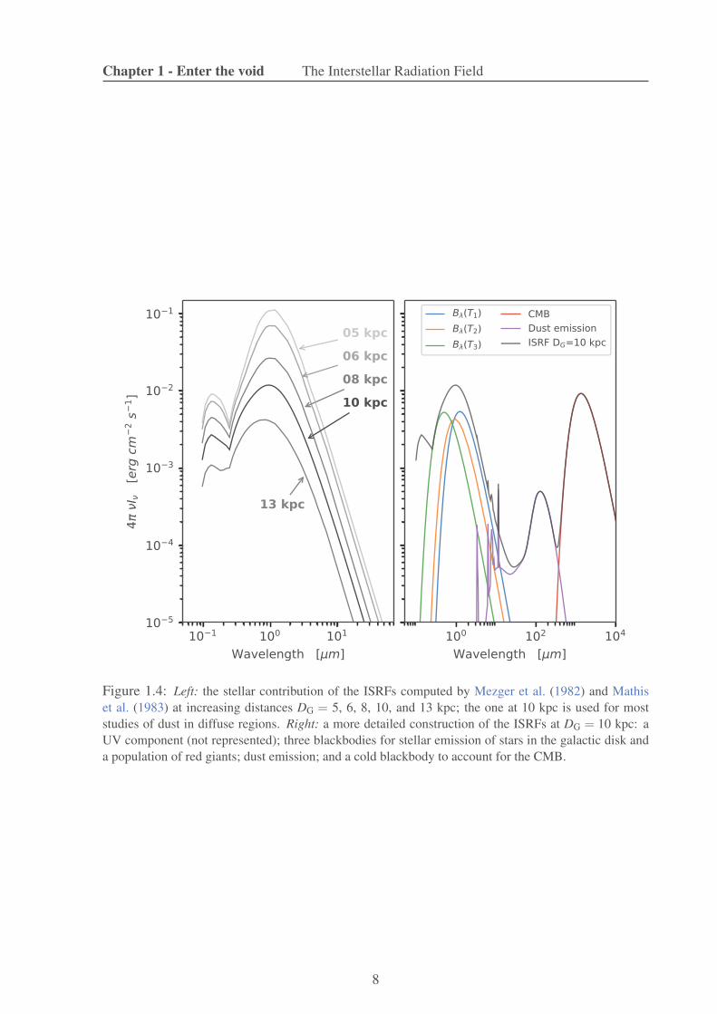
The gas and dust filling the ISM evolve under the conditions of the local interstellar radiationfield (ISRF), which determines their physical state. The ISRF is set by the surrounding stars3,as well as those distributed further throughout the galaxy. Their age, mass, or metallicity affectthis ISRF by the energy they provide. Dust emission depends on the shape and intensity of thesurrounding ISRF spectrum. To this day, the ISRF often used in dust modeling of diffuse regionshas been taken as that of the solar neighborhood. It is described with three main components(Figure 1.4):
• stars: the starlight from different stellar populations, modeled as a combination of severalblackbodies and a UV component. The three blackbodies have different temperatures(3000, 4000, and 7500 K) to depict two stellar populations in the disk, and a populationof red giant stars;
• dust emission: the resulting emission of dust grain heated by the photons at lower wave-lengths;
• cosmic microwave background (CMB): the remnant emission of the “first light” of theUniverse, modeled as a blackbody at ∼ 2.73 K;
Mezger et al. (1982) and Mathis et al. (1983) modeled this stellar emission as a function of thedistance to the galactic center, DG. In most studies, we use the reference at the distance DG =10 kpc, because it was approximately the estimated distance of our sun from the galactic centerat the time. Figure 1.4 shows these spectra at the different distances DG and the decompositionof the reference ISRF, based on the above description.
3Sometimes an active galactic nucleus can also be a significant contributor to dust heating, by affecting theISRF
7
Chapter 1 - Enter the void The Interstellar Radiation Field
Figure 1.4: Left: the stellar contribution of the ISRFs computed by Mezger et al. (1982) and Mathiset al. (1983) at increasing distances DG = 5, 6, 8, 10, and 13 kpc; the one at 10 kpc is used for moststudies of dust in diffuse regions. Right: a more detailed construction of the ISRFs at DG = 10 kpc: aUV component (not represented); three blackbodies for stellar emission of stars in the galactic disk anda population of red giants; dust emission; and a cold blackbody to account for the CMB.
8

2Interstellar Dust
Dust is a key component of the ISM. In this chapter, we will deepen the description of thephysical and chemical aspects of interstellar dust. This will lead us to understand how dustmodels are built and finally how can we detect dust in space.
2.1 Discovery, history and context
The idea of a component capable of absorbing light in space emerged about eighty years ago.Barnard (1910) noticed the obscuration of stars by “something” between them and us, the ob-servers. Trumpler (1930) established that this accentuated attenuation was different than thatdue to the simple diminution of light due to distance, as it decreased too rapidly. He analyzedpeculiar measurements, and concluded that small pieces of material were responsible of suchselective extinction. The reddening caused by dust, i.e. the shift in the emitted signal to shorter(redder) wavelengths was one of the essential clues of dust grain existence.
Dust is a crucial component of a galaxy for various reasons. First, it is a real chemistrylaboratory. For instance, grains hold heavy elements ejected from star cores. As such, it con-stitutes a reservoir of metals that eventually affects the evidence for evolution of a galaxy. Itis also important because of its cooling properties and its nature as a catalyst. Dust grains areformation sites for H2, mainly forming in the dense gas phase (Le Bourlot et al. 2012). Throughits absorbing properties, dust grains serve as cooling material of the ISM. Eventually, they allowfor molecular clouds to cool down to the temperature where gravitational collapse can happen,giving birth to stars. Dust also plays an important role in the energy distribution of the ISM.When heated by UV light from stars, electrons released by dust grains can be a major contrib-utor to heating the surrounding gas. The emission process from dust grains, that emit in theinfrared to release energy, is an important cooling mechanism, making dust grains a large con-tributor in the global energy budget and processing of a galaxy. Finally, dust grains can impactthe dynamics of the interstellar medium. For instance, they are sensitive to the magnetic fieldwhich can have an influence on dust grain orientation.
Studying dust is delicate, and the extent of our knowledge still promises critical progress.Observed dust properties are extremely dependant on the heating sources, and our understand-ing is thus linked to the observables. Nonetheless, more understanding of dust physics, along
9

Chapter 2 - Interstellar Dust Dust extinction
Figure 2.1: Left: Barnard68 molecular cloud, nicknamed Dark Cloud, observed at different wave-lengths. The absorption efficiency is clearly visible at smaller wavelength (blue), blocking the back-ground light coming from stars behind the cloud. Credit: ESO. Right: Lynds Dark Nebula 1251, anothermolecular cloud blocking the starlight. Credit: Lynn Hilborn
with progress in technology has lead to a list of observational constraints, whose terms will beexplained in the following sections, coupled with laboratories constraints:
• wavelength-dependent attenuation, and albedo;• features observed in extinction measurements: fixed position of the UV bump and vari-
able width;• polarization-dependent attenuation;• emission spectrum;• cosmic abundance of heavy elements;• optical and heating properties of condensed matter.
In the following, I describe more thoroughly these observables and dust properties.
2.2 Dust extinction
2.2.1 Some definitions
As aforementioned, one of the first measured characteristics of dust was its ability to absorblight. Dust “attenuates” the stellar light emitted in the UV (young objects) and optical (olderstars). Figure 2.1 illustrates this process in the Barnard 68 dark cloud. It is a dense cloud whichcompletely blocks the UV-optical light coming towards the observer. The multi-wavelengthpicture shows its efficiency depends on the wavelength.
Extinction measurements are usually done with the pair method. This consists of measuringthe signal of a star free of dust in its surroundings, and the dust-attenuated signal of a similar-type star, at a different position. The former gives the reference measurement for a wavelength.Knowing what the signal from the dusty star should be if no dust were present, we can derivethe amount that is removed by dust, and estimate a dust amount.
The intensity passing through a dust cloud at wavelength λ is determined by:
Iλ = Iλ0× e−τλ (2.1)
where Iλ0is the original intensity and τλ is the optical depth of the medium. The optical depth
characterizes the density, i.e. the number of particles, and the capacity of the dust (or gas) to
10

Chapter 2 - Interstellar Dust Dust extinction
extinguish light, with respect to their size and properties. It is usually defined with respect to theextinction in the V band (λ ∼ 0.55 µm). We can distinguish two extreme regimes described bythe optical depth: when τλ ≪ 1, we refer to the optically thin regime, i.e. few particles betweenthe source and the observer; when τλ ≫ 1, we refer to the optically thick regime. The originaland emerging intensities are related through the extinction term:
Aλ =−2.5log10(Iλ/Iλ0) (2.2)
which can eventually lead to an approximate relation between the extinction and the opticaldepth:
Aλ ∼ 1.086τλ (2.3)
The properties contained in the optical depth, τλ , depend on the extinction cross section, Cextand the grain radius a. In a homogeneous cloud of dimension l and particle density, nd:
τλ =Cext(a,λ ) nd l (2.4)
The grain properties are carried in the extinction efficiency, Qext:
Cext(a,λ ) = Qext(a,λ ) πa2 (2.5)
where πa2 represents the geometric cross section.
Absorption and Scattering The extinction is the cumulative effect of two processes calledabsorption and scattering. Equation 2.5 can be written:
Cext =Cabs +Csca and
Qabs ≡Cabs/πa2
Qsca ≡Csca/πa2 (2.6)
where Cabs and Csca are the absorption cross section and scattering cross section, respectively,and Qabs and Qabs are the absorption and scattering efficiencies, respectively.
Dust grains have the ability to absorb photons. This process leads to an increase of theinternal energy of the grain (equivalent to a raise of its temperature). Eventually, the grainre-emits the energy it absorbed, but at longer wavelengths, in the infrared.
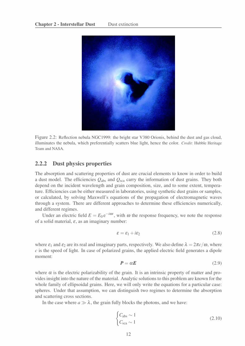
Scattering is the change of direction of propagation of a photon after it hits a dust grain.The photon has the same energy, but is not observable in the same direction. Scattering is mostvisible in what is called reflection nebulae, for which Figure 2.2 shows an example where acloud is illuminated by a star. The light we collect comes from the reverberation of the stellarlight on the dust particles of the cloud. Such situations provide measurements of the albedo,defined as the contribution of scattering compared to the total extinction:
albedo =Csca
Cext(2.7)
The albedo is thus an interesting property because it can be measured (e.g. Lewis et al. 2009),and provides an additional constraint for theoretical dust grain models. However, some works(e.g. Mathis et al. 2002) have showed that, even though we can measure extinction as well asand scattering in nebulae like that in Figure 2.2, constraining dust properties, and especiallytheir geometry, is very difficult and uncertain.
11
Chapter 2 - Interstellar Dust Dust extinction
Figure 2.2: Reflection nebula NGC1999: the bright star V380 Orionis, behind the dust and gas cloud,illuminates the nebula, which preferentially scatters blue light, hence the color. Credit: Hubble HeritageTeam and NASA.
2.2.2 Dust physics properties
The absorption and scattering properties of dust are crucial elements to know in order to builda dust model. The efficiencies Qabs and Qsca carry the information of dust grains. They bothdepend on the incident wavelength and grain composition, size, and to some extent, tempera-ture. Efficiencies can be either measured in laboratories, using synthetic dust grains or samples,or calculated, by solving Maxwell’s equations of the propagation of electromagnetic wavesthrough a system. There are different approaches to determine these efficiencies numerically,and different regimes.
Under an electric field E = E0 e−iωt , with ω the response frequency, we note the responseof a solid material, ε , as an imaginary number:
ε = ε1 + iε2 (2.8)
where ε1 and ε2 are its real and imaginary parts, respectively. We also define λ = 2πc/ω , wherec is the speed of light. In case of polarized grains, the applied electric field generates a dipolemoment:
PPP = αEEE (2.9)
where α is the electric polarizability of the grain. It is an intrinsic property of matter and pro-vides insight into the nature of the material. Analytic solutions to this problem are known for thewhole family of ellipsoidal grains. Here, we will only write the equations for a particular case:spheres. Under that assumption, we can distinguish two regimes to determine the absorptionand scattering cross sections.
In the case where a ≫ λ , the grain fully blocks the photons, and we have:
Cabs ∼ 1
Csca ∼ 1(2.10)
12

Chapter 2 - Interstellar Dust Dust extinction
If a ≪ λ , we call this regime the Rayleigh limit or the electric dipole limit. In this case, theelectric field appears uniform to the small grains, and the cross sections are:
Cabs =4πω
cIm(α)
Csca =8π
3
(ω
c
)4|α|2
(2.11)
And we can link this to the response ε (Equation 2.8):
Cabs = 18πε2
(ε1 +2)2 + ε22
Vλ
Csca = 24π3∣
∣
∣
∣
ε −1ε +2
∣
∣
∣
∣
2 V 2
λ 4
(2.12)
with V , the volume of grain material. We can note that, for very small grains, and still in thecase where a ≪ λ , as V → 0, Cabs ≫Csca: absorption prevails over scattering.In the same regime, at long wavelengths (λ → ∞ or ω → 0), we can write:
Cabs −−−→ω→0
fabsVλ 2
Csca −−−→ω→0
fscaV 2
λ 4
(2.13)
with fabs, fsca functions depending on the insulator or conductor nature of the grain:
fabs = fabs(ε0)
fsca = fsca(ε0)if insulator
fabs = f (1/σ0)
fsca = constantif conductor; σ0 is the grain conductivity
(2.14)
At long wavelengths, material with high σ0 will be a poor absorber as Cabs → 0. Figure 2.3shows an example of the extinction efficiencies for two types of grains, illustrating the λ−2 be-haviour. A very common example of this phenomenon is our daily blue sky, due to the Rayleighscattering at long wavelengths of sunlight by the particles in the atmosphere.
If the grain size is comparable to the wavelength, the previous solutions are not valid, andthe resolution of the Maxwell’s equations is not the same. The Mie theory, introduced by G. Mieand P. Debye around 1908, offers new solutions to this particular case. Then, the response of thegrain will depend on the ratio a/λ and its refractive index. As the incident electric wave travelsthrough the grain, the phase shift occurring after a distance a within the grain is an importantparameter to estimate the absorption and scattering cross sections of the grain.
We should also notice the importance of the spherical material assumption on the previousdevelopment. This is a strong simplification that could have important consequences whenconfronted with observations. The discrete dipole approximation (DDA; Purcell & Pennypacker1973) is an approach to avoid considering dust particles as spheroids. It is, however, verycomplex, and requires numerical calculations. The spheres approach is much faster, and is usedby most of the models to this day.
13

Chapter 2 - Interstellar Dust Dust extinction
Figure 2.3: Extinction efficiencies (absorption and scattering combined) for carbonaceous and silicategrains, in THEMIS (Jones et al. 2013; Köhler et al. 2014; Ysard et al. 2015)
2.2.3 Measurements of dust extinction
Empirically, variations of the extinction with wavelength can be summarized with an extinctioncurve. Cardelli et al. (1989) showed that the averaged extinction curves measured in the MilkyWay could be parameterized simply with
RV = AV/E(B−V ) (2.15)
The indices B and V refer to the bands at 0.44 and 0.55 µm, respectively; the reddeningE(B −V ) is the difference between the extinctions in these two bands. The same authorsshowed that the ratio Aλ/Aλref
can be completely parameterized by seven parameters, and ifRV is known, it can be parameterized by a one-parameter function.Figure 2.4 shows average extinction curves in the MW with varying RV) from Fitzpatrick(1999). A particular discrepancy between these curves can be noticed: the bump around4.5 µm−1 (∼ 217 nm). It is a well known feature of dust extinction, far from being wellunderstood, conveniently called the 2175 Å feature. Its position seems invariant but significantwidth variations have been observed (Beitia-Antero & Gómez de Castro 2017). Moreover, itappears absent in some lines of sight. If current evidence points towards a transition in graphiteor small aromatic hydrocarbons, its origin remains uncertain.
2.2.4 The Diffuse Interstellar Bands
The terms diffuse interstellar bands, or DIBs, refer to a series of extinction features, weak andbroad. Their width indicates that they are not atomic absorption lines but rather emerge fromlarge molecules. To this day, about 400 DIBs have been compiled, from 3900 Å to the NIR(Hobbs et al. 2009). It is important to admit that until very recently, none of these lines wereever assigned to a molecule. Figure 2.5 shows a compilation of several DIBs on the spectrum.
Although identified about 90 years ago, and classified as interstellar about a decade later(Heger 1922; Merrill & Wilson 1934; Merrill 1934) , only one idea has yet be proven right:buckminsterfullerene!
14

Chapter 2 - Interstellar Dust Dust extinction
Figure 2.4: A few extinction curves of the Galaxy from the work of Fitzpatrick (1999). They modeledextinction with a R (≡ RV) parametrization.
Figure 2.5: Cropped spectrum showing some Diffuse Interstellar Bands, after compilation from Jen-niskens & Desert (1994) work. Credit: http://www.kroto.info/dibs/
15

Chapter 2 - Interstellar Dust Dust emission
This cage-like molecule, composed of 60 carbon atoms and noted C60, resembles a football.In the late 80s, after a serendipitous discovery of C60 presence in space, its positively ionizedion was predicted to be a DIB carrier by Kroto & Jura (1992). Around 1995, two bands arestrongly suspected to be due to C+
60. In 2015, a team conclusively identifies C+60 as the carrier
of two DIBs, at 9577.4 and 9632.6 Å, thanks to an extremely low temperature experiment, thatallows the observations of molecules under 6 K (Campbell et al. 2015).
2.3 Dust emission
After absorbing the incident light in the UV and optical, dust grains re-emit this energy in theinfrared (from mid-infrared to sub-millimetric wavelengths). This emission also depends on thedust grain size and composition, and the shape and intensity of the incident interstellar radiationfield, its strength and hardness (see Section 1.3).
2.3.1 Thermal equilibrium
A grain large enough in a radiation field will absorb enough photons to be subject to a constantinput of energy, and will re-emit that energy at the same rate. In that particular state, the grainis in equilibrium with the heating rate1. The absorbed energy, Eabs, is:
Eabs =∫ ∞
04π nd πa2 Qabs(λ ,a) Jλ dλ (2.16)
where nd is the number density of grains, and Jλ is the mean intensity of the interstellar radiationfield. and we have energetic equality between emission and absorption, leading to:
∫ ∞
0Qabs(λ ,a) Jλ dλ =
∫ ∞
0Qabs(λ ,a) B(λ ,Td) dλ (2.17)
The term B(λ ,Td), or Bλ (Td) for simplification, is the Planck function at wavelength λ and dusttemperature, Td:
Bλ (Td) =2πc2
λ 5
1
ehc
kBλTd +1(2.18)
where c is the speed of light, h is the Planck constant, and kB is the Boltzmann constant.The grain emission however, is not a perfect blackbody, and is often referred to as a modified
blackbody. The modification lies in the emissivity of the dust grains. The surface brightness,Sλ , from a grain is:
Sλ = τλ Bλ (Td)
= nd πa2 Q Bλ (Td)
=Σd
mdπa2 Q Bλ (Td) with md =
43
πa3ρ
= κλ Σd Bλ (Td)
(2.19)
where τλ is the dust optical depth; nd is the number of grains, or dust column density; Σd is thedust surface density; ρ the grain density; md is the dust grain mass; and κλ is grain absorptioncross section per unit mass, characterizing the power of a dust grain to absorb/emit, at a givenwavelength.
1The equilibrium state can be achieved for small grain under the condition of a strong enough radiation field.However, it is usually admitted, from empirical situations, that mostly large grains are found to be in the equilibriumstate.
16

Chapter 2 - Interstellar Dust Dust emission
Wien’s law In the case of thermal equilibrium, it is possible to coarsely assess the peak ofradiation for large grain, using Wien’s law. It predicts:
λmax Td ∼ 3000 µm K (2.20)
where λmax is the wavelength at which the emission peaks. For instance, it means that dustgrains at temperature ∼ 30 K will have an emission peak at ∼ 100 µm.
Stefan-Boltzmann’s law In the case of a blackbody, the law of Stefan-Boltzmann predictsthat the power emitted is proportional to T4. In the case of grains in the equilibrium, i.e. emittingall the power they receive, we can connect this with the surrounding heating power, U (fromsurrounding stars; see Section 1.3):
U ∝ T 4+β (2.21)
where β is the spectral index of the dust grains. We therefore expect a large increase in lumi-nosity as the temperature rises. If we use the temperature of dust in the solar neighborhood, wecan derive a dust temperature knowing the local heating environment:
Td ∝ Td⊙
(
UU⊙
) 14+β
(2.22)
Recent results The space telescope Planck observed the universe from a few hundreds ofmicrons to centimeter wavelengths. The Planck collaboration modeled the dust emission withPlanck data and found Td between 16 and 24 K and β = 1.51 (Planck Collaboration et al. 2014,see also, Section 2.7).The Hi-GAL mission (Herschel Open Time Key-Project Molinari et al. 2010) mapped theGalactic plane (-1°< b < 1°) between 60 and 600 µm . Paradis et al. (2012) used this projectfor ISM studies and found dust temperatures between 16 and 25 K in this region, varying as thedistance from the Galactic center increases.
2.3.2 Stochastic heating
Thermal emission applies to grains whose size is sufficient to absorb photons continuously. Inthe opposite case, if the grain is too small that it absorbs photons irregularly, we refer to astochastic heating process. We no longer consider the power emitted by the dust grain as ablackbody, but as an average of the heat capacity of the grain, C(T ), over a timescale. Dueto absorption of individual photons, the grain temperature profile shows rapid spikes, and aslow decay toward lower temperatures. Every new photon absorbed creates a new raise intemperature, primarily due to a small heat capacity, as shown in Figure 2.6. It illustrates thetemperature in spikes, over a few lifetimes of grains at various sizes, and increasing time be-tween grain-photon interactions, τabs. It shows that, if the grain is too small, it undergoes strongpeaks in temperature, and a more gradual cooling, until it gets hit by a photon again. It depictsthe stochastic heating of small grains.
Instead of deriving an effective temperature, as for larger grains, we use a probability distri-bution of temperatures:
∫ ∞
0P(a,T ) dT with P(a,T ) = P(a,Tgrain ≤ T ) (2.23)
Figure 2.7 shows the peaks in temperature, for various grain sizes. We see that the smaller thegrain, the broader the temperature distribution. Only when the grain radius reaches a sufficientsize can we estimate a grain temperature.
17

Chapter 2 - Interstellar Dust Dust emission
Figure 2.6: Temperature fluctuations of dust grains, during ∼ 1 day. Each peak comes from a photonabsorption: if the grain radius a is too small, the grain undergoes a gradual cooling (bottom panel),instead of keeping a rather constant temperature (top panel). From Draine (2003a).
Figure 2.7: Temperature probability distributions of a few grains at different radii a. If the grains arebig enough, the probability is peaked, defining a unique grain temperature, as opposed to a small grain.
18

Chapter 2 - Interstellar Dust Dust emission
λ (µm) Identification
Known lines3.30 Aromatic C-H stretch6.22 Aromatic C-C stretch8.61 C-H bending, in-plane
Complexes
7.77.417 Aromatic C-C stretch7.56 Aromatic C-C stretch7.85 C-C stretch + C-h bending
11.311.23 C-H bending, out-of-plane11.33 C-H bending, out-of-plane
17.017.04 C-C-C bending17.38 C-C-C bending17.87 C-C-C bending
Empirical5.27 C-H bend + C-H stretch5.70 C-H bend + C-H stretch6.69 unknown13.5 C-H bending, out-of-plane14.2 C-H bending, out-of-plane15.9 unknown18.9 C-C-C bending
Table 2.1: Identification (or proposed specie, in italic) of some spectral lines, attempting todescribe the emission features in the range of 1−20 µm. Adapted from Draine & Li (2007)
2.3.3 Aromatic-rich (cyclic) carbonaceous
The emission in the mid-infrared, in the range ∼ 1− 20 µm, shows typical features that arisefrom vibration modes of cyclic hydrocarbon grains. They are characteristic of transitions ofthese large molecules and can be identified for the most part. Leger & Puget (1984) and Alla-mandola et al. (1985) identified the main features as:
• 3.3 µm: C - H stretching;• 6.2,7.7 µm: C - C stretching;• 8.6,11.3 µm: C - H bending.
However, the reality is more complicated. Some of these lines are complexes, encompassingthe combined emission of multiple signals. Some features are seen in laboratories but not inobserved spectra while some are seen in observations but their origins remain unknown. Draine& Li (2007) give a more complete description of these features and we gather a few of thecharacteristic features in Table 2.1.
Latest news: Stock & Peeters (2017) modeled the 7.7 µm complex with four Gaussian dis-tributions, instead of three as has usually been done. This would imply a fourth component inthe complex. That is not yet included in Table 2.1
19

Chapter 2 - Interstellar Dust Elemental abundances and dust composition
Element NX/NH Element NX/NH
C 2.69 10−4 Si 3.23 10−5
N 6.76 10−5 S 1.32 10−5
O 4.90 10−4 Mn 2.69 10−7
Mg 3.98 10−5 Fe 3.16 10−5
Table 2.2: Solar abundances adapted from Asplund et al. (2009).
2.4 Elemental abundances and dust composition
The dust emission and extinction are dependent on the chemical nature of the material. It isthus a necessity to know what dust grains are made of, in order to understand the interstellarobservables. Experimental measurements in laboratories allow us to derive optical and heatingproperties from grains of various sizes and nature.
The extinction theory and measurements we explained previously serve as a baseline toestimate the chemical composition of dust grains. From extinction measurements, it is possibleto estimate the total volume occupied by grains with respect to that of hydrogen atoms. Fromhere, a lower limit on the Mdust/MH (where Mdust is the total dust mass and MH is the hydrogenmass) ratio can be derived, which depends on the grain density ρ and a shape factor F :
Mdust
MH& 0.0056
(
1.2F
)(
ρ
3 g cm−3
)
(2.24)
However, H and He atoms locked in grains do not contribute a lot to the mass of these grains.To reach such ratio, it is essential to add element such as C, O, Mg, Si, S or Fe. Assumptionis made that the total interstellar abundance of an element is the sum of its quantities in the gasphase and in the solid phase. From spectroscopic measurements, we can measure the elementalabundances in the gas phase. The dust elemental abundance is thus the difference between thetotal and gas phase measurements:
The term [XH ]gas is called depletion of element X from the gas phase. It is estimated as the
difference between the observed abundance of the element X and that we would expect if theatoms were all in the gas phase:
[
XH
]
gas= log
(
N(X)
N(H)
)
−
[
XH
]
solar(2.25)
where N(X), N(H) are the volume densities if an element X and hydrogen, respectively, and[X
H ]solar is the depletion of the element X from the gas phase in the solar neighborhood. Stillusing spectroscopy, observations of absorption features, combined with molecular and atomicdata, allow the identification of the corresponding materials. For example, absorption lines at9.7 µm and 18 µm have been identified as Si−O and O−Si−O stretches. Combined withthe typical “broad and smooth” aspect of the absorption spectrum, we can strongly suspect thepresence of amorphous silicate in dust, instead of crystalline material. We are eventually ableto narrow down the possible solids describing dust grains: silicate in the form of pyroxene(MgxFe1−xSiO3) or olivine (Mg2xFe2−2xSiO4), oxides of metals (SiO2, MgO, Fe3O4), hydro-carbons, carbide (SiC)... There is a restriction, however, to the information spectra can give:absorption lines can only be recovered for atoms or small molecules. In the case of interstellardust, it is expected to find more complex material (like the silicates), and spectroscopic evidenceis therefore limited.
20

Chapter 2 - Interstellar Dust Grain sizes
Figure 2.8: Dust grains seen with electron microscopes. Left: Chondritic grain, i.e. found in a meteorite.Credit: Bradley et al. (2005). Middle: Aggregate of silicate and carbonaceous matter on a grain, probablychondritic. Credit: Volten et al. (2007). Right: Two images of SiC grains: (a) may be a fragment, while (b)appears to be a whole condensate. Credit: Heck et al. (2009)
Very few “real” interplanetary grains have been collected by spacecrafts in the Earth sur-roundings, or further away. They are used to conduct direct laboratories measurements. Figure2.8 shows a few example of these grains. The most striking information conveyed here is the(strongly) non-spherical aspect of the grains. Current models almost all assume spheres forefficient calculations. Such assumption underestimates the emissivity properties of dust grain,since their surface is, in fact, much larger. Also, these grains are very big compared to the limitsimposed on ISM dust grains. It is possible that interplanetary dust grains are conglomerates ofsmaller interstellar grains.
New Horizons Student Dust Counter: during its flyby to Pluto, the instrument designed tocollect and analyze dust grains on the fly was hit by only "six particles per cubic mile"; this isan indication on how rare the grains can be in our very close neighborhood.
2.5 Grain sizes
Minimal and maximal dust grain sizes are estimated through many observational constraints.Based on extinction measurements, scattering of visible light and polarization observations,we know that grains must cover a large size distribution, from ∼ 0.01 to 0.2 µm. Emissionfeatures tell us that smaller grains are required to reproduce observations, with sizes down to∼ 0.003 µm. Recent dust models, detailed in the following section, use that information tocreate dust grain size distributions matching those measurements.
2.6 Dust grain models
Modeling dust emission and extinction is critical, and the properties and methods describedabove are used to build dust models. At each grain size and grain composition, we know thelaws predicting the extinction and emission, through theoretical calculations and laboratorymeasurements. Despite this information, to this day, there is not a unique model able to repro-duce the observations. However, using this knowledge, numerous studies have focused on theinverse problem: with extinction and emission measurements from nearby and distant galaxies,what can we derive on the composition and size distribution of dust grains from regions faraway?
21

Chapter 2 - Interstellar Dust Dust grain models
In Section 2.3.1, we saw that the emission of large grains in thermal equilibrium can beapproximated by a blackbody, with a few changes. To build simple dust models taking intoaccount only the large grain distribution, we can change the term κλ with different approaches,which modify the blackbody spectrum. Two “common” methods to attribute a change to κλ arethe Simple Modified Blackbody (SMBB)and the Broken-Emissivity Modified Blackbody (BE-MBB). Gordon et al. (2014) defined properties of the SMBB as:
κSMBBλ = κeff
λ0
(
λ
λ0
)−β
κBEMBBλ = κeff
λ0
1
λ−β10
λ−β1 if λ < λb
λ(β2−β1)b λ−β2 if λ ≥ λb
(2.26)
β typically ranges between 1 and 3, according to laboratories measurements, and most studiesassumed a value of 2 (Henning & Mutschke 1997; Demyk et al. 2017). This is directly relatedto the Qabs and Qsca properties (see Section 2.2).
However, we know from MIR emission that there must be smaller grains that are responsi-ble for the emission features at shorter wavelengths. To model those, we need a complete modelwith grain size distributions. The first dust model was developed in the 1940s (Oort & van deHulst 1946). The solid phase was, at the time, described as ‘smoke’, an ensemble of smallparticles of a few microns in radius, and smaller. This smoke would contribute to the globalextinction visible in space.Mathis et al. (1977) used power-law size distributions to describe silicate and graphite popu-lations to fit the observed extinction. After pioneer work from Platt (1956) and Donn (1968),the PAHs became acknowledged as responsible of many extinction and emission features, andmodels started adding a third component to the dust composition: Desert et al. (1990); Draine& Li (2001); Li & Draine (2001); Weingartner & Draine (2001); Zubko et al. (2004); Draine &Li (2007).In most cases, these models vary from one another by the size distributions they use. Thedifference in composition can be minor (e.g. different extinction efficiencies) or carry greaterconsequences, like the use of different carbonaceous molecules: amorphous versus crystalline(graphite, diamond). All of these models manage to fit the Milky Way dust extinction and emis-sion, and lie within acceptable abundances. The free parameters vary from a model to another,and it is an important point to study: which parameter are degenerate? Which parameters arekept fixed and why? These questions are the very reasons for the work presented in this thesis.
In this thesis, we will use three of these models in particular. A more explicit description isneeded, in order to understand the differences that exist between models.
2.6.1 Draine & Li (2007)
The Draine & Li (2007) model (hereafter, DL07) originally stems from the model built byDraine & Lee (1984). It is a natural extension of the first graphite-silicate model, as newconstraints brought new insights on dust modeling. Cross sections used in DL07 come fromDraine & Lee (1984), who showed that their composition could fit the dust observables. Asignificant input was done by Draine & Li (2001) and Li & Draine (2001) by adding PAHs tothe carbon grain distribution, after identification of their emission features in the mid-IR. Draine& Li (2001) also updated heat capacities. The “current” DL07 model uses an updated sizedistribution following the extensive work from Weingartner & Draine (2001). Minor changesbased on more recent work and new assumptions bring revisions to this model, which is, to thisday, the most frequently used in IR dust modeling.
22

Chapter 2 - Interstellar Dust Dust grain models
2.6.2 Compiègne et al. (2011)
The Compiègne et al. (2011) model, or for further simplification, the DustEM model, alsofollows a family of dust models, its parent being that from Desert et al. (1990). The Desert et al.(1990) model described dust with three components: PAHs, very small grains, and big grains.The DustEM model is more precise in its description, and uses five components; the PAHpopulation is split between neutral and ionized molecules; the carbonaceous grains, amorphous,are divided between a small and a large populations; finally, the silicate component only useslarge grains. The small grain sizes are computed with a log-normal distribution while the largecarbon and silicate grains are determined to have a power-law distribution. The carbonaceouspopulations are based on Zubko et al. (1996) and the silicate properties come from Draine &Lee (1984); they are “astronomicalised” to be compatible with sub-mm observations and aretherefore more empirical, based on works from Li & Draine (2001), Draine (2003b) and Draine& Li (2001). An important point is the common spectral index of both large carbonaceous andsilicate grains. The PAHs cross sections are slightly modified from Draine & Li (2007).
2.6.3 THEMIS
Another model has recently been developed by Jones et al. (2013). Based on a series of newlaboratory measurements from Jones (2012c,d,a,e,b), and updated by Köhler et al. (2014) andYsard et al. (2015), it is named THEMIS for The Heterogeneous Evolution dust Model at theIAS2. Its particularity, besides taking into account laboratory data, is to take into account thePAH-like material in the form of mantles around the dust grains. In this model, the smallestgrains are only aromatic-rich, while large carbonaceous grains have an aliphatic-rich core, cov-ered by an aromatic mantle, just like silicate-core grains. The difference between aromatic andaliphatic lies in the crystal organization, leading to more or less H atoms. Further work havealso added ices to this model: it enables grain aggregation in very dense regions, such as molec-ular clouds.Because it is heavily based on laboratory data, this model is not exactly fit to the same observa-tions as the other models. However, Ysard et al. (2015) adjusted the dust masses and density tobe able to reproduce the different ISM phases in the MW.The model is therefore described by two grain populations, split into four components; thecarbonaceous material is divided between a small grain population, aromatic-rich, and a largegrain population with aliphatic cores and aromatic mantles. The metals are locked into twosilicate-based compositions: pyroxene (SiO3)2 and olivine (SiO4).
2.6.4 Calibration
Most dust models are calibrated on measurements done in the MW, and more precisely in thelocal neighborhood. It is where our constraints have the lower uncertainties, even though it rep-resents only one sample. For example, the DustEM model uses a combination of extinction andemission to adjust their model. The extinction curve is that of RV = 3.1 from Fitzpatrick (1999).The total emission spectrum used to calibrate DustEM is a compilation of many observationsfrom the near-IR to the submillimetric wavelengths. It covers a large portion of the sky at highgalactic latitude (|b| > 15°), in order to select the diffuse ISM of our Galaxy (see Compiègneet al. 2011, for a compilation).Additional information is used from depletion measurements. It helps to estimate a limit on the
2Institut d’Astrophysique Spatiale (Paris, France)
23

Chapter 2 - Interstellar Dust Observations and Instruments
quantity of each element to put in the grain composition. Jenkins (2009) carried out extensivework on depletions which are used today.Other galaxies have been used to constrain models. For instance, Weingartner & Draine (2001)built dust models, in particular size distributions based on fits of the Magellanic Clouds, twonearby galaxies (see Section 4).
2.7 Observations and Instruments
To confront theoretical models with “reality”, we need measurements that will constrain theemission, extinction and abundances in samples of galaxies of various shapes, dynamics, orages... Here is a short history of space telescopes used in IR studies.
Infrared measurements have to be taken from space. The atmosphere surrounding the Earthblocks infrared photons and therefore prevents ground based IR measurements. The InfraredAstronomical Satellite (IRAS; Neugebauer et al. 1984) was launched in 1983, for a missionthat lasted 10 months. It was the first space observatory to observe the full-sky at four in-frared wavelengths: 12, 25, 60 and 100 µm. The Cosmic Background Explorer (COBE) waslaunched in 1989; its main goal was to observe the microwave background emission, but two ofits instruments (DIRBE and FIRAS) took measurements of the sky in infrared wavelengths. In1995, the European Space Agency (ESA) launched the Infrared Space Observatory (ISO), forobservations between 2.4 and 240 µm.
More recent space observatories have had an incredible impact on modern astrophysics,and this thesis is mainly based on measurements from these telescopes. The level of precisionin IR observations was largely increased with the Spitzer Space Telescope (Werner et al. 2004)launched in 2003, whose main mission ended in 2009 (the “warm” mission is still ongoing at thetwo shortest wavelengths). It was not a full-sky survey, but pointed observations, as was ISO.Spitzer carried 3 instruments to orbit. Among these, two are for photometry, IRAC (InfraredArray Camera; Fazio et al. 2004) and MIPS (Multiband Imaging Photometer for Spitzer; Riekeet al. 2004). IRAC photometric bands are centered on 3.6, 4.5, 5.8, and 8.0 µm, and MIPS bandson 24, 70, and 160 µm. The spectrometer, IRS (Infrared Spectrograph; Houck et al. 2004),covered 5 to 38 µm, with both high and low resolutions. The science questions that Spitzer wasbuilt to tackle were, among others, star formation or young stellar objects as well as dust, givenits spectral coverage. Some programs used Spitzer, making significant contributions in dustanalysis in nearby galaxies. The SINGS consortium (Kennicutt et al. 2003) took measurementsof 75 galaxies and focused on their IR emission and star formation properties. Two programswere meant to study in detail regions of the Small Magellanic Cloud (SMC), a nearby dwarfgalaxy, in photometry and spectroscopy (S3MC, S4MC; Bolatto et al. 2007; Sandstrom et al.2012). The SAGE surveys (SMC and LMC; Meixner et al. 2006; Gordon et al. 2011) were keysprojects of the Spitzer program and are used in numerous studies.
The Herschel Space Observatory (Pilbratt et al. 2010) was launched in 2009, and remainedfunctional until 2013, working as a pointed instrument as well, and operating from the L2 point.Its photometry channels covered 6 bands, split between two instruments. PACS (Photoconduc-tor Array Camera and Spectrometer; Poglitsch et al. 2010) covered 70, 100, and 160 µm, andSPIRE (Spectral and Photometric Imaging Receiver ; Griffin et al. 2010) covered 250, 350, and500 µm. PACS also allowed for spectroscopy between 55 and 210 µm a moderate resolution;the HIFI spectrometer worked between 157 and 625 µm. Since its coverage was in the IR,Herschel was almost fully dedicated to the study of interstellar dust. Numerous studies haveused Herschel state-of-the-art resolutions and a lot of studies continue. One of the main pro-grams useful for us is HERITAGE (Meixner et al. 2013, 2015), which focused on dust in the
24
Chapter 2 - Interstellar Dust Observations and Instruments
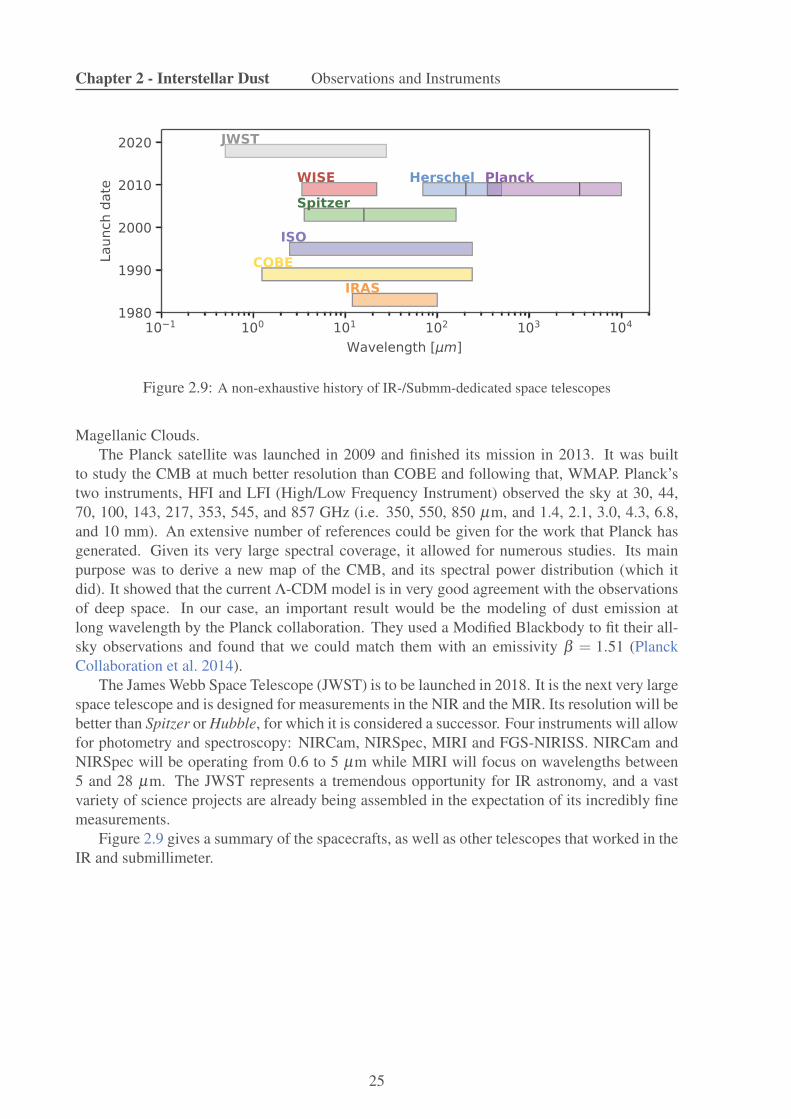
Figure 2.9: A non-exhaustive history of IR-/Submm-dedicated space telescopes
Magellanic Clouds.The Planck satellite was launched in 2009 and finished its mission in 2013. It was built
to study the CMB at much better resolution than COBE and following that, WMAP. Planck’stwo instruments, HFI and LFI (High/Low Frequency Instrument) observed the sky at 30, 44,70, 100, 143, 217, 353, 545, and 857 GHz (i.e. 350, 550, 850 µm, and 1.4, 2.1, 3.0, 4.3, 6.8,and 10 mm). An extensive number of references could be given for the work that Planck hasgenerated. Given its very large spectral coverage, it allowed for numerous studies. Its mainpurpose was to derive a new map of the CMB, and its spectral power distribution (which itdid). It showed that the current Λ-CDM model is in very good agreement with the observationsof deep space. In our case, an important result would be the modeling of dust emission atlong wavelength by the Planck collaboration. They used a Modified Blackbody to fit their all-sky observations and found that we could match them with an emissivity β = 1.51 (PlanckCollaboration et al. 2014).
The James Webb Space Telescope (JWST) is to be launched in 2018. It is the next very largespace telescope and is designed for measurements in the NIR and the MIR. Its resolution will bebetter than Spitzer or Hubble, for which it is considered a successor. Four instruments will allowfor photometry and spectroscopy: NIRCam, NIRSpec, MIRI and FGS-NIRISS. NIRCam andNIRSpec will be operating from 0.6 to 5 µm while MIRI will focus on wavelengths between5 and 28 µm. The JWST represents a tremendous opportunity for IR astronomy, and a vastvariety of science projects are already being assembled in the expectation of its incredibly finemeasurements.
Figure 2.9 gives a summary of the spacecrafts, as well as other telescopes that worked in theIR and submillimeter.
25

Chapter 2 - Interstellar Dust Observations and Instruments
PART I − TAKE AWAY
This Part has introduced us to the characteristics of interstellar dust. Here are a few keypoints to remember for the purpose of this thesis:
• a galaxy is filled with numerous and diverse components: old and young stars, hotand cold gas, diffuse and dense clouds of dust... which are all studied through light;
• the multiple objects in a galaxy contribute to the energy budget, and create availablephotons travelling through space and defining the Interstellar Radiation Field;
• dust can be observed through a few processes:
– dust absorbs and scatters the UV and visible light, through a global processthat we define as the extinction; its properties can be summarized in anextinction curve; this extinction curve has typical features like the 217 nmbump or the DIBS, whose variations and origins are uncertain;
– dust re-emits this energy in the IR through the process of emission; the emis-sion spectrum depends on the grain characteristics: large grains are inthermal equilibrium and their emission is similar to a modified blackbody,while small grains are stochastically heated and their emission showsfeatures in the MIR and PAH features;
– dust composition can be estimated through spectroscopy measurements in thegas phase; polarization is also a dust characteristic that can be observed;
• dust models adjusting all these observables are created to match our observationsand derive dust properties in nearby and distant galaxies.
We will use these models to fit the IR emission in nearby galaxies in an applicationdescribed in the Part II.
26

Part II
Modeling dust emission in the MagellanicClouds
27


3Fitting the IR emission in nearby galaxies
3.1 Context of this study
Dust plays a fundamental role in the evolution of a galaxy. It has a large impact on the thermo-dynamics and chemistry processes by catalyzing molecular gas formation (e.g. H2 formationsites). It can be a gas tracer when the gas-to-dust ratio is known. It reflects the chemical historyof a galaxy... To comprehend the dust impact on other processes and features in the ISM, it isof crucial importance to understand its physical state and composition, including minimal andmaximal grain sizes, as described by dust models presented in Section 2.6.
All these models vary from one to another by the definition of dust composition, size dis-tribution of grains, and laboratory-based data for optical properties, and are not necessarilyconstrained by the same observational references. As described in Chapter 2.7, the widelyaccepted description of dust involves two main chemical entities: carbonaceous grains, whichusually show both amorphous and aromatic structures, and silicate grains, with metallic-elementinclusions to agree with the observed abundances.
Section 2.7 presented the progress made in IR observations, from IRAS to Herschel andfuture JWST. In the ultraviolet, continued observations and analysis of extinction (Cardelli et al.1988, 1989; Mathis 1990; Fitzpatrick & Massa 2005; Cartledge et al. 2005; Gordon et al. 2003,2009) and depletions (Jenkins 2009; Tchernyshyov et al. 2015) have shown that large variationsin dust properties exist from one line of sight to the next, and between galaxies.
Although we may have identified common behaviour with different models, the same mod-els do not agree on all deduced properties (e.g., dust masses). It is difficult to determine whetherthe differences between dust studies arise from the intrinsic descriptions of the dust models, orthe statistical treatment of the fitting algorithm, or both. In this study published as a paper (Chas-tenet et al. 2017), we use current dust grain models to fit the MIR to sub-millimeter observationsof two nearby galaxies. Our goal is to quantitatively measure the discrepancies between themodels used in a common fitting scheme, and assess which part of the SEDs can be reproducedbest with a given set of physical inputs. To do so, we base our effort on the work of Gordonet al. (2014). In their study, they focused on fitting three models to the Herschel HERITAGEPACS and SPIRE photometric data: the Simple Modified BlackBody, the Broken EmissivityModified BlackBody and the Two Temperatures Modified BlackBody (SMBB, BEMBB and
29

Chapter 3 - Fitting the IR emission in nearby galaxies Studying nearby galaxies
TTMBB, respectively). They identified a substantial sub-millimeter excess at 500 µm, in twonearby galaxies, presented below, likely explained by a change in the emissivity slope. Theybuilt grids of spectra, varying parameters for a given model (e.g., for the SMBB model, they al-low the dust surface density, the spectral index, and the dust temperature to vary). They adopteda Bayesian approach to derive, for each spectrum, the multi-dimensional likelihood assuminga multi-variate Normal/Gaussian distribution for the data to assess the probability that a set ofparameters fit the data. Their residuals and derived gas-to-dust ratio favor the BEMBB model,which best accounts for the sub-millimeter excess. We use the same statistical approach in thisstudy. We present the two galaxies studied here, the Magellanic Clouds, before explaining thedata in Section 4.3. Because we extend the observational constraints to shorter wavelengths,we must account for smaller dust grains and “full” models, and we make use of the DustEMtool 1 (Compiègne et al. 2011) to build our own grid of physical dust models (Section 5). Wethen compare the different models used based on residual characteristics (Section 6) and derivephysical properties and interpretations (Sections 7 and 8).
3.2 Studying nearby galaxies
The closest galaxy to study is, of course, the one we live in. However, despite obvious highresolution, observing a galaxy from within comes with numerous drawbacks. For instance,the confusion along the line of sight, for any object in the MW lower than a latitude of ∼30°, is extremely important. Observations in the galactic disk are very complicated becausemost of the objects are found in this disk, all mixed together. A similar confusion can befaced when observing external galaxies. Because of our position in the MW, observations ofother galaxies may exhibit a foreground, a signal that is not part of the studied object. Inthe IR, this foreground is the emission of the Galactic cirrus, the atomic gas floating in theMW, and confusing observers. However blaming it all on our Galaxy would be a shame: aconfusing background also makes observations difficult. It is the signal emitted by faint anddistant galaxies, called the Cosmic Infrared Background. This mixture of signals coming fromdifferent parts in space, along a single line-of-sight, cannot be avoided, and only reduced.
Another kind of problematic mixture happens in observations of nearby galaxies. Whenthe spatial resolution is too coarse, the signal contained in that single fraction is the sum ofmultiple objects in a single pixel. Studying nearby galaxies is a way to decrease the impact ofthat problem: the closer the galaxy, the finer the spatial resolution, and the lower the number ofobjects in a single pixel.
Studying these galaxies, however, holds for an argument of statistical sample. Being re-stricted to only our Galaxy does not allow for general theories. The high variety of properties innearby galaxies is a tremendous advantage in constraining our models: different shapes, dynam-ics, or ages lead to different evolution scenarios, with various galaxy properties. In the case ofthe ISM, studying galaxies other than the MW gives us access to multiple types of environmentin which the dust and gas evolve. Since they are correlated with the star formation and age ofa galaxy, we do not expect to see the same properties when it comes to a galaxy different fromthe MW. Using this different stages helps us to understand the life-cycle of ISM componentswithin the galaxy, and how it changes from one galaxy to the next.
It also allows different approaches to study a galaxy. One can either consider its smallercomponents: when the resolution is good enough, we can distinguish sub-parts of the galaxysuch as bubbles, filaments, star formation regions... These parts have individual properties than
1http://www.ias.u-psud.fr/DUSTEM/
30

Chapter 3 - Fitting the IR emission in nearby galaxies Studying nearby galaxies
Figure 3.1: Artist view of the Milky Way (left), and pictures of the Andromeda (middle) and Triangulum(right) galaxies. Credit: NASA - Lorenzo Comolli - Robert Gendler
can be of interest as such. On the other hand, one can choose to treat the galaxy as a whole,with average properties. Going further, we might even link the detailed behavior of a galaxywith its global characteristic. In doing so, studying nearby galaxies can be of great help whendistant galaxies cannot be resolved.
In general, “nearby galaxies” refers to galaxies within the Local Group. It covers a radiusof ∼ 1.5 Mpc around the MW, including about 54 galaxies. It includes three spiral galaxies,represented in Figure 3.1, the Milky Way, the Andromeda Galaxy (M31) and the TriangulumGalaxy (M33). Most of the other objects are irregular and dwarf galaxies, satellites of the MilkyWay or Andromeda, including the Magellanic Clouds, two galaxies of particular interest in thisthesis.
31

Chapter 3 - Fitting the IR emission in nearby galaxies Studying nearby galaxies
32

4The Magellanic Clouds: close neighbors
4.1 Description of the Clouds
In the surroundings of the MW, two small galaxies dance around. They can be seen with thenaked eye, from the South hemisphere: the Small and Large Magellanic Clouds (together, theMCs; see Figure 4.1); although seen since ancient times, their name is a reference to the navi-gator Ferdinand Magellan who mention them in his travel journal. The Small Magellanic Cloud(SMC) is at 62 kpc from us (Graczyk et al. 2014) while the Large Magellanic Cloud (LMC)stands closer, at about 50 kpc (Keller & Wood 2006; Walker 2012). They are among the closestgalaxies to us, classified as dwarf irregular galaxies, and are objects of particular significancefor many reasons developed below, when it comes to studying the ISM.
With such proximity to us, the level of details achieved with recent instruments (Spitzer orHerschel) is unprecedented. With the resolution of Herschel, we can resolve down to ∼ 13 pcin the LMC and ∼ 17 pc in the SMC. As a comparison, studies have shown that the typical ISMstructure in the dense phase is of a few tens of parsecs (Roman-Duval et al. 2010). The MCsare therefore among the best nearby galaxies to study in terms of resolution. Because of theirposition (galactic latitude of ∼ 30−45°; ascension and declination coordinates: 00 52 38.0 -72 48 01 and 05 23 34.6 -69 45 22 for the SMC and LMC, respectively) the MCs suffer fromless foreground confusion than other galaxies at lower latitude. Close to the galactic pole, thezodiacal light contamination is also less substantial than in other observations.
With a lower metallicity than the MW, of respectively 1/2 Z⊙ and 1/5 Z⊙ for the LMC andSMC (Russell & Dopita 1992; Rolleston et al. 2002), the MCs are expected to show differencesin behaviour than that we would expect in a galaxy similar in metallicity to the MW. Withless metals available compared to the MW, the star formation history and composition of dustis bound to be different from what we observe in our Galaxy. In particular, in the scope ofthis work, the metallicity directly impacts the observed properties of the ISM. The elementsavailable for dust formation depend on the generations of stars that made possible heavy elementproduction, from the nucleosynthesis occurring in their dense cores.
Using H I gas measurements, we find evidence that the two galaxies are in interaction (Put-man et al. 2003; Brüns et al. 2005). The observable track left by this interaction is called theMagellanic Stream (for an extensive review, see D’Onghia & Fox 2016). In the SMC, this
33

Chapter 4 - The Magellanic Clouds: close neighbors Interest of the MCs
30-Dor
N11B
LMC4
Bar
N44
! 5.5°
N83A
Wing
Bar
N66A
NGC456
N88A
NGC602
SMCB2
Lirs36
SMCB1
! 3.5°
Figure 4.1: Left: The Large Magellanic Cloud. Credit: NASA, JPL-Caltech, M. Meixner and SAGE team.Right: The Small Magellanic Cloud. Credit: ESA, NASA, JPL-Caltech, STScI. The red regions indicate afew interesting spots in the galaxies, often studied and/or particularly bright.
LMC SMC
Stellar mass 3.9 109 M⊙ 3.0 108 M⊙
HI mass 4.4 108 M⊙ 4.0 108 M⊙
Total mass 1.7 1010 M⊙ 2.4 109 M⊙
Table 4.1: A few mass indicators in the LMC and SMC. The dust mass is omitted on purpose (Stan-imirovic et al. 2004; Brüns et al. 2005; Harris 2007; van der Marel & Kallivayalil 2014).
stream causes the gas and the stars to behave dynamically different, unlike that usually seen inother, more quiescent galaxies.
In Table 4.1 we gather a few indicators of masses in the galaxies. Despite an order ofmagnitude of difference in their total dust masses, the SMC atomic gas mass is quite close tothat of the LMC. The extent of the H I distribution around the SMC is characteristic of thisgalaxy: although many galaxies shows a broad distribution, this is more visible in the SMC.
4.2 Interest of the MCs
Observations show that the infrared SEDs of the MCs differ from those seen in the Milky Way(MW). At (sub-)millimeter and centimeter wavelengths, dust is well modeled by a blackbodyspectrum modified by a power-law (see Section 2.6). Many investigations have identified thistrend by pointing out “excess” emission in the far-infrared (FIR) to radio wavelengths (e.g.,Galliano et al. 2003, 2005; Bot et al. 2010; Israel et al. 2010; Gordon et al. 2010; Galliano et al.2011; Gordon et al. 2014). In those models, it means that the spectral emissivity index β islower in the MCs than in the MW. This excess had also been reported in the MW, althoughmore mildly by Reach et al. (1995), who suggested this excess in the MW comes from colddust. They rejected this hypothesis as the dust mass needed to account for such an emission(with dust at very low temperature) would be too high to be realistic, and violate elementalabundances. The current theory points toward different a power-law (i.e., different spectralindices) in the expression of the emissivity, in different wavelength ranges (e.g., a ‘broken-
34

Chapter 4 - The Magellanic Clouds: close neighbors Data used in this study
emissivity’ modified blackbody model). Another kind of excess has been identified at 70 µm,with respect to the expected emission from MW-based dust models. The studies of Bot et al.(2004) and Bernard et al. (2008) linked this excess to a different size distribution and abundanceof the very small grains whose emission is dominant at these wavelengths. The infrared peak(100 µm 6 λ 6 250 µm) also varies between the MW and the MCs and tends to be localized atshorter wavelengths in the SMC. This tendency may be due to the more intense radiation fieldsin the SMC.
Besides being close and offering good resolution, the MCs therefore seem to be good can-didates to test the limits of our dust models.
4.3 Data used in this study
In this study, I fit the dust emission of the MCs. The MIR, FIR, and sub-millimeter images usedin this study are taken from the Spitzer SAGE-SMC (Surveying the Agents of Galaxy Evolu-tion; Gordon et al. 2011) and SAGE-LMC (Meixner et al. 2006) Legacies and the HerschelHERITAGE Key Project (The Herschel Inventory of the Agents of Galaxy Evolution; Meixneret al. 2013, 2015). The SAGE observations were taken with Spitzer Space Telescope (Werneret al. 2004) photometry instruments: the Infrared Array Camera (IRAC; Fazio et al. 2004) pro-vided images at 3.6, 4.5, 5.8 and 8.0 µm and the Multiband Imaging Photometer for Spitzer(MIPS; Rieke et al. 2004) providing images at 24, 70, and 160 µm. The observations cover a∼ 30 °2 region for the SMC and ∼ 50 °2 for the LMC. Data in the FIR to sub-millimeter weretaken with PACS (Photoconductor Array Camera and Spectrometer; Poglitsch et al. 2010) andSPIRE (Spectral and Photometric Imaging Receiver; Griffin et al. 2010) on board the HerschelSpace Observatory (Pilbratt et al. 2010), providing images at 100, 160, 250, 350, and 500 µm.The observations cover the same regions as the Spitzer data.
I used the combined Spitzer and Herschel sets of bands to cover the IR spectrum. Thecombined bands are from IRAC 3.6, 4.5, 5.8, and 8.0 µm, MIPS 24 and 70 µm, PACS 100and 160 µm, and SPIRE 250, 350 and 500 µm. Thanks to the custom de-striping techniquesused to process the HERITAGE data (see Meixner et al. 2013, for details), the PACS 100 datacombines the resolution of Herschel with the sensitivity of IRAS 100. Similarly, the PACS 160image was merged with the MIPS 160 image.
Like Gordon et al. (2014), first, all the images were convolved using the Aniano et al. (2011)kernels to decrease the spatial resolution of all images to the resolution of the SPIRE 500 µmband of ∼ 36′′. Next, the foreground dust Milky Way dust emission was subtracted. To do so, webuilt a MW dust foreground map using the MW velocity H I gas maps from Stanimirovic et al.(2000) for the SMC and Staveley-Smith et al. (2003) for the LMC. To convert the velocity gasmaps to a dust emission map, I used the Compiègne et al. (2011) model. I derived conversioncoefficients from H I column to MW dust emission, and subtracted the resulting maps from thedata.
After this processing, the PACS observations show a gradient across the images. I removedthis gradient by subtracting a two-dimensional surface, estimated from background regions inthe images. Regions outside the galaxies (and bright sources) were chosen to evaluate a “back-ground” plane that was then subtracted from all the images. For the LMC, the observations didnot extend beyond the full disk and this introduced a larger uncertainty in the final backgroundsubtracted images. The SMC observations extend beyond the galaxy and we have access toregions on the images fully outside the galaxy. Finally, I rebinned the images to have a pixelscale of ∼ 56′′ that is larger than the resolution of the SPIRE 500 µm band to provide nominally
35

Chapter 4 - The Magellanic Clouds: close neighbors Data used in this study
Figure 4.2: The Small Magellanic Cloud seen with Spitzer at 3.6, 4.5, 5.8, 8.0, 24 and 70 µm andHerschel at 100, 160, 250, 350 and 500 µm.
independent measurements for later fitting. Figures 4.2 and 4.3 shows the final data used in the11 bands.
36

Chapter 4 - The Magellanic Clouds: close neighbors Data used in this study
Figure 4.3: The Large Magellanic Cloud seen with Spitzer at 3.6, 4.5, 5.8, 8.0, 24 and 70 µm andHerschel at 100, 160, 250, 350 and 500 µm.
37

Chapter 4 - The Magellanic Clouds: close neighbors Data used in this study
38

5Tools and computation
To create the model SEDs, I used DustEM. To find the best fit in each pixel, or compare modelsto observations, I used the SED fitting tool: DustBFF. We will overview here in more detailsboth tools and the work done.
5.1 DustEM
The DustEM tool (Compiègne et al. 2011) outputs emission and extinction curves calculatedfrom dust grains properties. For each grain type, properties like the scattering and absorptionefficiencies Qext(λ ,a) and Qsca(λ ,a), and the heat capacities C(λ ,a) are used. Each modelavailable explicitly specifies the minimal and maximal grain size amin, amax and the size dis-tribution law to adopt for each grain component. Finally, astronomical data like the full ISRFspectrum is used as well. I use the DustEM IDL wrapper1 to generate full model grids with alarge number of emission spectra. The wrapper forward-models the observations by multiply-ing the model SED with transmission curves. I used two dust models in this study (see 2.6 formore details) based on the work from Compiègne et al. (2011) and Jones et al. (2013) updatedby Köhler et al. (2014) and Ysard et al. (2015). Here, we remind briefly the reader what thecomponents of these models are.
The model from Compiègne et al. (2011) (MC11) is a mixture of PAHs, both neutral andionized (cations), small and large amorphous carbonaceous grains (SamC and LamC, respec-tively; Zubko et al. 1996) with different size distributions, and amorphous silicate grains (aSil;Draine & Lee 1984), that is, a total of five independent components. In my fitting, I chose to useonly a single PAH population, by summing the ionized and neutral species together. Given theshape of the emission spectra from the charged and neutral PAHs, the broad-band observationscould not constrain them independently. I also tied (by summing) the big grains (BGs) together,originally described by both large carbonaceous and amorphous silicates. At λ > 250 µm,the emissivity law of both carbon and silicate grains in this model is the same (β ∼ 1.7−1.8).Hence, they cannot be discriminated from their emission alone and allowing them to vary wouldresult in the fitting arbitrarily choosing one or the other type of grains. Their variations with the
1available at http://dustemwrap.irap.omp.eu/
39
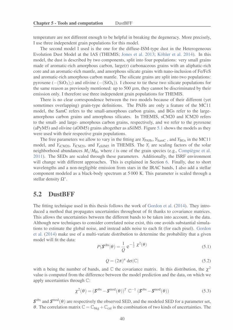
Chapter 5 - Tools and computation DustBFF
temperature are not different enough to be helpful in breaking the degeneracy. More precisely,I use three independent grain populations for this model.
The second model I used is the one for the diffuse-ISM-type dust in the HeterogeneousEvolution Dust Model at the IAS (THEMIS; Jones et al. 2013; Köhler et al. 2014). In thismodel, the dust is described by two components, split into four populations: very small grainsmade of aromatic-rich amorphous carbon, large(r) carbonaceous grains with an aliphatic-richcore and an aromatic-rich mantle, and amorphous silicate grains with nano-inclusion of Fe/FeSand aromatic-rich amorphous carbon mantle. The silicate grains are split into two populations:pyroxene (−(SiO3)2) and olivine (−(SiO4)). I choose to tie these two silicate populations forthe same reason as previously mentioned: up to 500 µm, they cannot be discriminated by theiremission only. I therefore use three independent grain populations for THEMIS.
There is no clear correspondence between the two models because of their different (yetsometimes overlapping) grain-type definitions. The PAHs are only a feature of the MC11model, the SamC refers to the small-amorphous carbon grains, and BGs refer to the large-amorphous carbon grains and amorphous silicates. In THEMIS, sCM20 and lCM20 refersto the small- and large- amorphous carbon grains, respectively, and we refer to the pyroxene(aPyM5) and olivine (aOlM5) grains altogether as aSilM5. Figure 5.1 shows the models as theywere used with their respective grain populations.
The free parameters we allow to vary in the fitting are YPAHs, YSamC , and YBGs in the MC11model, and YsCM20, YlCM20, and YaSilM5 in THEMIS. The Yi are scaling factors of the solarneighborhood abundances Mi/MH, where i is one of the grain species (e.g., Compiègne et al.2011). The SEDs are scaled through these parameters. Additionally, the ISRF environmentwill change with different approaches. This is explained in Section 6. Finally, due to shortwavelengths and a non-negligible emission from stars in the IRAC bands, I also add a stellarcomponent modeled as a black-body spectrum at 5 000 K. This parameter is scaled through astellar density Ω∗.
5.2 DustBFF
The fitting technique used in this thesis follows the work of Gordon et al. (2014). They intro-duced a method that propagates uncertainties throughout of fit thanks to covariance matrices.This allows the uncertainties between the different bands to be taken into account, in the data.Although new techniques to consider correlated noise exist, this one avoids substantial simula-tions to estimate the global noise, and instead adds noise to each fit (for each pixel). Gordonet al. (2014) make use of a multi-variate distribution to determine the probability that a givenmodel will fit the data:
P(SSSobs|θ) =1Q
e−12 χ2(θ) (5.1)
Q = (2π)n det|C| (5.2)
with n being the number of bands, and C the covariance matrix. In this distribution, the χ2
value is computed from the difference between the model prediction and the data, on which weapply uncertainties through C:
χ2(θ) = (SSSobs −SSSmod(θ))TC−1 (SSSobs −SSSmod(θ)) (5.3)
SSSobs and SSSmod(θ) are respectively the observed SED, and the modeled SED for a parameter set,θ . The correlation matrix C=Cbkg+Ccal is the combination of two kinds of uncertainties. The
40

Chapter 5 - Tools and computation DustBFF
Figure 5.1: Compiègne et al. (2011) (MC11 model, left) and THEMIS (right) emission spectra, forU=1 (from Mathis et al. (1983)) and NH = 1020 H cm−2. The difference between these two models arethe total number of components and optical and heating properties. The stellar component is a scaledblackbody at 5 000 K.
41

Chapter 5 - Tools and computation DustBFF
Figure 5.2: SPIRE500 image of the LMC showing the regions defined to determine the backgroundcorrelation matrix Cbkg, marked by red circles.
correlation of the background from band to band is an empirical measure made over each band,and each element of the matrix is defined as:
(Cbkg)2i j =
∑Nk (S
ki −〈Si〉)(Sk
j −〈S j〉)
N −1. (5.4)
with Skx, the value of the kth in the xth band, and 〈Sx〉, the average background value of the
xth band. In order to avoid contamination from the actual signal one tries to model, Cbkg iscalculated from regions outside of the galaxy. Figure 5.2 shows a example of regions (circles)chosen in the LMC. The higher the number of pixels, N, counted as part of the background, thebetter will be Cbkg estimation.
The errors made on the observations themselves are part of the Ccal matrix. It is calculatedas:
(Ccal)i, j = Smodi (θ)) Smod
i (θ)) (Muncorr +Mcorr) (5.5)
The matrices Muncorr and Mcorr are determined from the detailed calibration work done foreach instrument. For ‘uncorrelated’ errors, we usually refer to the characteristic of repeatabilityof measurements. This term describes how stable a measurement is in instrument units at high
42
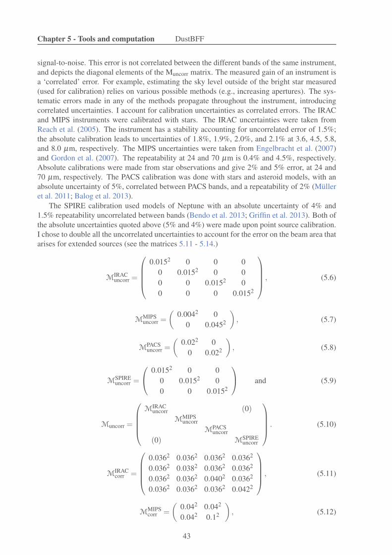
Chapter 5 - Tools and computation DustBFF
signal-to-noise. This error is not correlated between the different bands of the same instrument,and depicts the diagonal elements of the Muncorr matrix. The measured gain of an instrument isa ‘correlated’ error. For example, estimating the sky level outside of the bright star measured(used for calibration) relies on various possible methods (e.g., increasing apertures). The sys-tematic errors made in any of the methods propagate throughout the instrument, introducingcorrelated uncertainties. I account for calibration uncertainties as correlated errors. The IRACand MIPS instruments were calibrated with stars. The IRAC uncertainties were taken fromReach et al. (2005). The instrument has a stability accounting for uncorrelated error of 1.5%;the absolute calibration leads to uncertainties of 1.8%, 1.9%, 2.0%, and 2.1% at 3.6, 4.5, 5.8,and 8.0 µm, respectively. The MIPS uncertainties were taken from Engelbracht et al. (2007)and Gordon et al. (2007). The repeatability at 24 and 70 µm is 0.4% and 4.5%, respectively.Absolute calibrations were made from star observations and give 2% and 5% error, at 24 and70 µm, respectively. The PACS calibration was done with stars and asteroid models, with anabsolute uncertainty of 5%, correlated between PACS bands, and a repeatability of 2% (Mülleret al. 2011; Balog et al. 2013).
The SPIRE calibration used models of Neptune with an absolute uncertainty of 4% and1.5% repeatability uncorrelated between bands (Bendo et al. 2013; Griffin et al. 2013). Both ofthe absolute uncertainties quoted above (5% and 4%) were made upon point source calibration.I chose to double all the uncorrelated uncertainties to account for the error on the beam area thatarises for extended sources (see the matrices 5.11 - 5.14.)
MIRACuncorr =
0.0152 0 0 00 0.0152 0 00 0 0.0152 00 0 0 0.0152
, (5.6)
MMIPSuncorr =
(
0.0042 00 0.0452
)
, (5.7)
MPACSuncorr =
(
0.022 00 0.022
)
, (5.8)
MSPIREuncorr =
0.0152 0 00 0.0152 00 0 0.0152
and (5.9)
Muncorr =
MIRACuncorr (0)
MMIPSuncorr
MPACSuncorr
(0) MSPIREuncorr
. (5.10)
MIRACcorr =
0.0362 0.0362 0.0362 0.0362
0.0362 0.0382 0.0362 0.0362
0.0362 0.0362 0.0402 0.0362
0.0362 0.0362 0.0362 0.0422
, (5.11)
MMIPScorr =
(
0.042 0.042
0.042 0.12
)
, (5.12)
43

Chapter 5 - Tools and computation DustBFF
Figure 5.3: Representation of the DustBFF outputs: the ’max’ corresponds to the maximum likelihood,’exp’ to the weighted average likelihood. A few realizations are shown as well.
MPACScorr =
(
0.12 0.12
0.12 0.12
)
, (5.13)
MSPIREcorr =
0.082 0.082 0.082
0.082 0.082 0.082
0.082 0.082 0.082
and (5.14)
Mcorr =
MIRACcorr (0)
MMIPScorr
MPACScorr
(0) MSPIREcorr
. (5.15)
The DustBFF tool outputs the n-D likelihood function of the fits, and marginalizes it on eachparameter space to create 1D likelihoods. Several estimates can then be used. The ‘max’ value isdefined as the maximum likelihood, or sometimes traditionally referred to as the χ2; it reflectsthe closest model to the observations, and in this study I use it for residual calculations (seeSection 6). The expectation (‘exp’) value translates more the whole likelihood in the sense thatit is a weighted average. It has the advantage of giving a more global picture of the likelihoodfunction. A very useful approach is to randomly extract multiple values of a likelihood function.This ‘realization’ method reflects the shape of the function and the fitting noise. This will beused to study parameter behavior, and namely derive dust masses. These outputs are representedon a schematic view in Figure 5.3.
44

Chapter 5 - Tools and computation Model (re-)calibration
5.3 Model (re-)calibration
Since I want to investigate the differences between two dust-grain models independently of thefitting algorithm, it is critical to make sure that they share the same calibration. Moreover, thiscalibration should be made using the same measurements with the same technique. Usually,dust grain models are calibrated to reproduce the diffuse MW dust emission (e.g., Boulangeret al. 1996) and extinction, with constraints on elemental abundances from depletion measure-ments (e.g., Jenkins 2009; Tchernyshyov et al. 2015). However, they often do not share thesame calibration technique or the same constraint measurements.
MC11 and THEMIS size distributions are calibrated on the diffuse extinction in the MW.Measurements at high Galactic latitude from the Cosmic Background Explorer (COBE; Ben-nett et al. 1996), coupled with the Wilkinson Microwave Anisotropy Probe (WMAP; Jarosiket al. 2011) and Infrared Space Observatory (ISO; Mattila et al. 1996) trace the global SEDof dust emission. It was correlated with H I measurements and is expressed in flux units perhydrogen atom. Hence, in both models, the dust grain ‘masses’ are given as dust-to-hydrogenratios Mdust/MH. The total dust mass in each model implies a hydrogen-to-dust ratio that variesfrom one model to the other. Although each model fits the MW dust emission at high latitude,given their different dust descriptions, they do not necessarily share the same gas-to-dust ratio.However, this should be a reference point in calibrating dust models as this can be measuredwith other methods. In the MW, I follow the value of Gordon et al. (2014) and set the diffuseMW hydrogen-to-dust ratio at 150 (derived from Jenkins 2009, for F∗ ∼ 0.36).
To ensure that both models produce the same result when fitted to the MW diffuse ISM,I “recalibrate” the models using the ISO, COBE, and WMAP measurements of the local ISMas described in Compiègne et al. (2011). I do not take into account the 0.77 correction forthe ionized gas in order to be consistent with the depletion work of Jenkins (2009), whichdoes not correct the ionized gas contribution. I integrated this spectrum in the Spitzer andHerschel photometric bands and obtained a SED whose values are shown in Table 5.1. ThePACS and SPIRE values are very close to those displayed in Gordon et al. (2014) (Section 5.1in their paper).
I used the DustBFF fitting technique to scale the full spectrum of each model to the SEDdescribed in Table 5.1 and found the factor that gave the adopted gas-to-dust ratio of 150. Idid not allow the grain species to vary from one another, and I chose to keep the same ratiosbetween populations as described by the model. I set the ISRF at U = 1, that is, the sameused for the model definition. The fits thus consist of adjusting the global emissivity, andscaling the total emission spectrum. I built a different correlation matrix for the estimated fluxuncertainties from the observing instruments quoted. Following Gordon et al. (2014), I assumed5% correlated and 2.5% uncorrelated uncertainties at long wavelengths for the COBE, FIRAS,and DIRBE instruments (accounting for PACS and SPIRE bands). I presumed a 10% error forboth correlated and uncorrelated uncertainties at short wavelengths given the resolution of ISO(accounting for IRAC and MIPS bands). I derived a scaling factor that is the result of the fit ofthe models. The final correction factors are 1.6 and 2.42 for the whole spectrum of THEMISand the MC11 model, respectively. These factors aim at self-calibrating the models to givethe same gas-to-dust ratio of 150 for the same MW SED. This step is crucial as the goal is tocompare two models, independently of the fitting method, for which differences are eliminatedby the use of a common fitting procedure. It should be noted that, if the first step aims at arigorous fit to the MW SED, the second step’s goal is to adjust the GDR and therefore movesaway from a good fit.
I convert the emission output from DustEM 4π νIν , in erg s−1 cm−2 (H cm−2)−1 to surface
45

Chapter 5 - Tools and computation Model (re-)calibration
Bands Diffuse ISM Bands Diffuse ISM
IRAC3.6 0.00235 PACS100 0.714IRAC4.5 0.00206 PACS160 1.55IRAC5.8 0.0134 SPIRE250 1.08IRAC8.0 0.0431 SPIRE350 0.561MIPS24 0.0348 SPIRE500 0.239MIPS70 0.286
Table 5.1: The values of the local diffuse ISM integrated in the Spitzer and Herschel bands,used for calibration, in MJy sr−1 ×10²⁰ H atom−1.
brightness units, expressed in MJy sr−1, with the scaling factors as follows:
Sλ = 4π νIν ×2.65 1021 ×λ ×
1.6 if we use THEMIS
2.42 if we use MC11. (5.16)
46

6Model comparison
I vary a number of dust model parameters that affect the SED shape and fit these new spectra tothe data. In this study, I mainly examine dust emission when it is illuminated by different ISRFmixtures. At higher ISRFs, we expect the IR peak to shift to shorter wavelengths. I focus onthis behaviour after considering the shape of global SEDs in the MCs. In all cases, I vary the Yiparameters, which adjust each grain abundance. I also change the ISRF intensity, scaled by thefree parameter U . In the whole study, I use the standard radiation field defined by Mathis et al.(1983). The U = 1 case corresponds to the solar neighborhood ISRF U⊙. In one case only, Ivary the small grain size distribution. Throughout the fitting, I do not change the large grainsize distributions, and therefore assume no change between the MW and the MCs, regardingthis aspect.
I choose to fit each pixel that is detected at least 3σ above the background in eight bands(IRAC8.0, MIPS24 and MIPS70, PACS100 and PACS160 and all SPIRE bands): I do notimpose the detection condition at 3.6, 4.5, and 5.8 µm as these bands can include a significantcontribution from stars. I do include all the IRAC observational data in the fitting. In thefollowing, the ‘faint’ or ‘bright’ aspect of a pixel is based on its emission at 500 µm.
To study the fits quality, I use fitting residuals. They illustrate how the models match thedata and are expressed as the error (data−model)/data.
Figure 6.1 shows fitting results for two pixels in the SMC, one with faint emission (left) andone with bright emission (right), for THEMIS only. This figure gives an idea of the differentmodel variations that are described in the following sections.
6.1 Using a single ISRF
I first used the models with a single ISRF environment. This simply means that each spectrum iscalculated from the emission of grains illuminated by a single ISRF, the strength of which varies.I do not change the shape or hardness of the ISRF. In Figure 6.2, I show the distribution offractional residuals expressed as (data−model)/data, in the SMC (top) and the LMC (bottom)for the two different models. The red bars shows the results for THEMIS and the purple bars,the MC11 model.
47
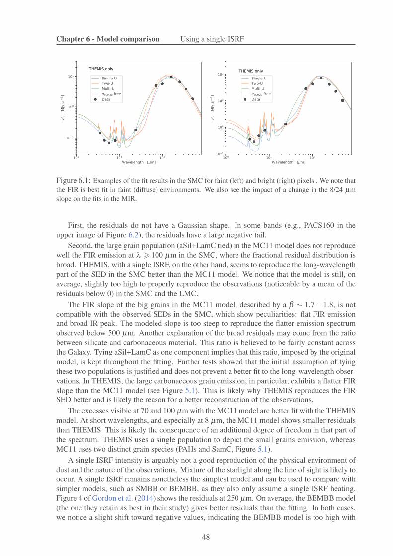
Chapter 6 - Model comparison Using a single ISRF
Figure 6.1: Examples of the fit results in the SMC for faint (left) and bright (right) pixels . We note thatthe FIR is best fit in faint (diffuse) environments. We also see the impact of a change in the 8/24 µmslope on the fits in the MIR.
First, the residuals do not have a Gaussian shape. In some bands (e.g., PACS160 in theupper image of Figure 6.2), the residuals have a large negative tail.
Second, the large grain population (aSil+LamC tied) in the MC11 model does not reproducewell the FIR emission at λ > 100 µm in the SMC, where the fractional residual distribution isbroad. THEMIS, with a single ISRF, on the other hand, seems to reproduce the long-wavelengthpart of the SED in the SMC better than the MC11 model. We notice that the model is still, onaverage, slightly too high to properly reproduce the observations (noticeable by a mean of theresiduals below 0) in the SMC and the LMC.
The FIR slope of the big grains in the MC11 model, described by a β ∼ 1.7− 1.8, is notcompatible with the observed SEDs in the SMC, which show peculiarities: flat FIR emissionand broad IR peak. The modeled slope is too steep to reproduce the flatter emission spectrumobserved below 500 µm. Another explanation of the broad residuals may come from the ratiobetween silicate and carbonaceous material. This ratio is believed to be fairly constant acrossthe Galaxy. Tying aSil+LamC as one component implies that this ratio, imposed by the originalmodel, is kept throughout the fitting. Further tests showed that the initial assumption of tyingthese two populations is justified and does not prevent a better fit to the long-wavelength obser-vations. In THEMIS, the large carbonaceous grain emission, in particular, exhibits a flatter FIRslope than the MC11 model (see Figure 5.1). This is likely why THEMIS reproduces the FIRSED better and is likely the reason for a better reconstruction of the observations.
The excesses visible at 70 and 100 µm with the MC11 model are better fit with the THEMISmodel. At short wavelengths, and especially at 8 µm, the MC11 model shows smaller residualsthan THEMIS. This is likely the consequence of an additional degree of freedom in that part ofthe spectrum. THEMIS uses a single population to depict the small grains emission, whereasMC11 uses two distinct grain species (PAHs and SamC, Figure 5.1).
A single ISRF intensity is arguably not a good reproduction of the physical environment ofdust and the nature of the observations. Mixture of the starlight along the line of sight is likely tooccur. A single ISRF remains nonetheless the simplest model and can be used to compare withsimpler models, such as SMBB or BEMBB, as they also only assume a single ISRF heating.Figure 4 of Gordon et al. (2014) shows the residuals at 250 µm. On average, the BEMBB model(the one they retain as best in their study) gives better residuals than the fitting. In both cases,we notice a slight shift toward negative values, indicating the BEMBB model is too high with
48

Chapter 6 - Model comparison Using multiple ISRFs
respect to the observations. Yet, their results better match the data. This is likely due to the factthat the FIR slope can be directly adjusted using the β2 parameter in each pixel independently.
6.2 Using multiple ISRFs
The next level of complexity for the heating environment is to use two ISRFs. In this case,I consider two components of dust: I calculate the emission of each grain population whenirradiated by two ISRFs with different strengths, which leads to a “warm” dust and a “colder”one, and then mix the spectra with a fraction f warm:
Iν = ∑X
YX
(
f warmIXwarm
ν +(1− f warm)IXcold
ν
)
, (6.1)
where X = aSilM5; lCM20;sCM20 (THEMIS). The fraction parameter YX is identical for allgrain populations. Effectively, we have two parameters Uwarm and Ucold, that both scale up anddown the ISRF. It physically means that I model two dust masses Mwarm
dust and Mcolddust , instead
of a single effective dust mass as in Section 6.1. The IXwarm
ν and IXcold
ν refer to the dust SEDsheated by Uwarm and Ucold, respectively, with Ucold < Uwarm. Meisner & Finkbeiner (2015)used a similar approach to fit the Planck HFI all-sky maps combined with IRAS 100 µm. Theyshowed that this provides better fits in the wavelength range (100 - 3 000 µm) than a simplemodified blackbody.
Finally, one can use a more complicated combination of ISRFs. Thus, I also follow thework of Dale et al. (2001) in which the final SED is a power-law combination of SEDs atvarious ISRFs, integrated over a range of strengths:
dMd(U) ∝ U−αISRFdU, 10−1U⊙ ≤U ≤ 103.5U⊙ (6.2)
The αISRF coefficient is the parameter that regulates the weight of strong/weak ISRFs in themixture used to irradiate the dust in a multi-ISRF model. A low αISRF gives more weight tothe high ISRFs. I allow the αISRF parameter to vary between 1 and 3, as suggested by previousstudies (e.g. Bernard et al. 2008).
Figure 6.1 gives a representation of the differences on the dust emission brought by changingthe ISRF. The results are shown for THEMIS, in a faint (left) and bright (right) pixels (basedon SPIRE500 emission). In Figure 6.1, we note that the use of multiple ISRFs leads to a bettermatch of the 24 µm data. In the faint pixel, the emission in the IRAC bands is dominated bystarlight and not extremely sensitive to small carbon grains, except at 8.0 µm. The differencesin the fits in a faint or bright pixel could mean that diffuse regions are better reproduced byTHEMIS than brighter regions, which are most likely denser. In these regions, dust may besignificantly different in terms of dust properties, and a fixed dust grain model may not beappropriate.
In Figure 6.3, I show the residuals for THEMIS used in a two-ISRF environment (orangebars), and THEMIS and MC11 models in a multi-ISRF environment (green bars). As a refer-ence, I keep the results for the simplest THEMIS model (i.e., “single ISRF”; red bars). The FIRresiduals for the MC11 model do not show improvements with respect to those of a single ISRFenvironment (Figure 6.2, purple bars). At λ 6 24 µm, it follows THEMIS with the same envi-ronment, and hence does not have strong assets. At long wavelengths (λ > 100 µm), THEMIS,in the two environments described in this section, has residuals centered on 0, and are no longershifted below 0 as is the case for the single-ISRF model. This is most visible in the SMC (top
49

Chapter 6 - Model comparison Using multiple ISRFs
Figure 6.2: Histograms of fractional residuals for the MC11 (purple) and THEMIS (red) models ina single ISRF environment in the SMC (top) and the LMC (bottom). On the upper panel, trianglesand squares show the residuals for the same faint and bright pixels, respectively, as Figure 6.1; colorscorrespond to the models.
50

Chapter 6 - Model comparison Varying the small grain size distribution
panel). In the LMC (bottom panel), the single-ISRF model provides a relatively good fit, andthe improvements of the other models are less significant.
We can see the multi-ISRF model improves the fits at 5.8 µm 6 λ 6 70 µm in both theSMC and LMC. Mixing the dust heated by different ISRFs notably helps to match the dataat 8.0 and 24 µm. Using only two ISRF components does not seem enough, and this modelreproduces the same SED as a single-ISRF model at these wavelengths. The efficiency of usinga power-law is due to its effect on the 8/24 µm slope. By steepening it, it matches both theNIR and MIR data better. After this section, I no longer use the MC11 model. It suffers fromstrong divergence with the data and the effects brought by using more than a single ISRF do notimprove the quality of the fits.
6.3 Varying the small grain size distribution
We saw in Section 6.1 that a single ISRF does not match the data at short wavelengths very well:the residuals are broad and mostly negative (i.e., the model overpredicts the observations). InSection 6.2, I tested different environment changes to try to better account for the shape ofSEDs. But variations in grain size distribution can also have an impact on the shape of thedust emission. In THEMIS, the small grain size distribution is described by a power-law, partlydefined as dn/da ∝ a−αsCM20 , where a is the grain radius. In order to obtain better fits at thesewavelengths (3.6, 4.5, 5.8, 8.0, 24 µm), I investigate the impact of changing the sCM20 sizedistribution. In this approach, I keep a single ISRF but allow the αsCM20 parameter to vary.
In Figure 6.4, I show the residuals for this variation (light blue) in the SMC (top), and theLMC (bottom). In both galaxies, the fits at λ > 70 µm are not improved by this model comparedto a simple single ISRF (red bars). However, the residuals show that this model matches thedata better at short wavelengths, particularly in the SMC. The peak of the residuals are centeredon 0 and the residuals are less broad. This improvement is due to the change in the shape ofthe SED brought by the free parameter αsCM20. When αsCM20 decreases, the 8/24 µm slopesteepens. This helps to decrease the model values in the MIR. In a more physical aspect, whenαsCM20 is lower, the sCM20 mass distribution is rearranged and it leads to fewer very smallgrains.
The SMC and the LMC exhibit two different fitting results to the αsCM20 parameter, whichcan vary between 2.6 and 5.4. In the LMC, I find 〈αsCM20〉 ∼ 5.0, that is, the default value setin the THEMIS model to reproduce MW dust emission. In the SMC, I find 〈αsCM20〉 ∼ 4.0,with αsCM20 < 4.0 in bright regions (e.g., N66, N76, N83) or H II regions (e.g. S54). Theimprovement in the residuals comes from a better fit in these regions allowed by a different SEDshape in the IRAC and MIPS24 bands. Bernard et al. (2008) found that changing the power-lawcoefficient of the VSG of the Desert et al. (1990) model from 3.0 to 1.0 helps matching the dataand decreases the 70 µm excess, and the estimate goes in the same direction.
51

Chapter 6 - Model comparison Varying the small grain size distribution
Figure 6.3: Histograms of fractional residuals for THEMIS in a two-ISRF (orange bars) and a multi-ISRF (green bars) environment, in the SMC (top), and the LMC (bottom). For reference, THEMIS in asingle ISRF is shown in red bars.
52

Chapter 6 - Model comparison Varying the small grain size distribution
Figure 6.4: Histograms of fractional residuals for THEMIS in a single ISRF environment with a changeof the sCM20 size distribution (blue bars) in the SMC (top) and the LMC (bottom). For reference,THEMIS in a single ISRF is shown by red bars.
53

Chapter 6 - Model comparison Varying the small grain size distribution
54

7Dust properties inferred from modeling
Based on the results from the residual study (described in Section 6), I focus on the outputfrom the models that best reproduces the observations: THEMIS, in a two-ISRF environment, amulti-ISRF environment, and with αsCM20 free in a single-ISRF environment. I investigate thedust properties that are inferred that way.
7.1 Parameter spatial variations
I investigated the spatial variations of the parameter distribution by building parameter maps.The maps show strong differences from one model to another.
In Figures 7.1 and 7.2, I show the maps of the resulting scaling factors Yi for i=aSilM5,lCM20 and sCM20 (first, second, and third rows, respectively), in the SMC (top) and theLMC (bottom), for the two-ISRF, multi-ISRF, and αsCM20 free models (first, second, and thirdcolumns, respectively). The first and third rows (YaSilM5 and YsCM20) show the most strikingvariations. I only display meaningful pixels, that is, pixels where the result is higher than itsuncertainty, in color. For example, in the upper-right corner of Figure 7.1 (top), the very fewpixels displayed are the only significant pixels. I emphasize that the same pixels were fitted ineach case, and the discrepancies in the images come from variations in results. As a guide, thefaint gray patterns show all fitting pixels, including those with no good fits.
The silicate fitting, discussed in the following section (7.2), is strongly affected by the choiceof heating environment in both galaxies, although it is particularly noticeable in the SMC. Usinga multi-ISRF model reduces the number of poorly-constrained fits (i.e., with an upper limit).On the other hand, the αsCM20 free model leaves an extensive portion of the galaxy with un-constrained fits (not-shown pixels, with an upper limit on silicate abundances, that is, a largeuncertainty). The results in the LMC appear to be less variable from one model to another. Asseen from the residuals, the models match the LMC observations better than they match theSMC observations. This difference may come from the constraints put on the silicate spectrumshape, which seem to vary from one model to another. In the case of a multi-ISRF model, theemission of silicates is significant at 70 µm. The total flux in this band (MIPS70) thus has astronger silicate contribution. This means the silicate spectrum has one more constraint, at ashorter wavelength. This could be the reason for the improved fitting result compared to other
55

Chapter 7 - Dust properties inferred from modeling Silicate grains abundance
models where the MIPS70 bands are mostly constrained by smaller grains. The more “con-stant” results in the LMC likely come from the fact that they are closer to MW SEDs, uponwhich the dust grain models are calibrated.
The YlCM20 fitting results (second rows) do not show strong variations from one model toanother. In the SMC, all the pixels are fitted, and the discrepancies are actual fitting results. Inthe LMC, the results are once again less variable and seem to be trustworthy. I compared theresulting fitting parameter maps to those derived by Paradis et al. (2009). They used the Desertet al. (1990) model to fit the Spitzer emission of the MCs. It should be noted that their study andours do not use the same model nor the same fitting technique. They found that the YPAH/YBGratio is higher in the LMC bar, in both cases, with a single ISRF and with a multi-ISRF model.Such a behavior does not appear in these maps. I do not find any spatial trend in the distributionof YsCM20/(YaSilM5 +YlCM20). However, it is difficult to rigorously establish a comparison aseven the grain species are not defined in the same way in the different studies.
The YsCM20 fitting results are sensitive to the model. The results from the αsCM20 free modelshows regions with more sCM20 that can be correlated to some extent with H II regions, tracedby Hα (Gaustad et al. 2001). The distribution of the YsCM20 parameter in the last column isdue to the change of size distribution of the small grains. Changing the power-law coefficientof the sCM20 size distribution has one main advantage: it steepens the 8/24 µm slope. Thishelps to fit the 8 and 24 µm bands in the SMC, as shown in Figure 6.4. However, it raises theIR emission peak of the small grains. In regions where αsCM20 is very low, the IR peak can befitted by the sCM20 species, and requires only a small contribution of the large grains.
7.2 Silicate grains abundance
In Section 7.1, we saw that the silicate grains component is highly model-dependent, and thatmost of the pixels are not fit with a reliable uncertainty (Figure 7.1). The figure shows that theSMC and the LMC do not exhibit the same results, and that the SMC is more sensitive to themodel than the LMC.
In both galaxies, I find pixels that show a likelihood where the silicate component is onlyconstrained as an upper limit (i.e., all models below a given abundance of silicates have thesame probability). From the likelihoods in the pixels with an unconstrained value of the silicatecomponent, I can quote a 3-σ upper limit for the absence of the silicate in the fitting. This upperlimit is YaSilM5 ∼ 100.4MaSilM5
⊙/MH, in both the SMC and the LMC.In Figure 7.3, I show likelihoods of the free parameters YaSilM5, YlCM20, YsCM20, and Ω∗ in
two pixels: one that shows a good constraint on the amount of silicates (blue line), and oneconstraining YaSilM5 with an upper-limit only. The results in the two galaxies differ: in theLMC, ∼ 10% of the pixels show this kind of likelihood; in the SMC, more than 50% do notshow a fully-constrained fit. In Figure 7.4, I display two representations of the SED fitting in thesame pixels used for the likelihoods of Figure 7.3. I used ‘realizations’ of the likelihoods (as inGordon et al. 2014, see Section 6). The realizations are a weighted sample from the likelihood.The opacity of the color in Figure 7.4 represents the probability of the value in the SED (themore opaque the color, the higher the probability). The top panel shows a very broad region withdecreasing probability (i.e., increasing transparency) towards the observational values, whereasthe bottom panel depicts a constrained fit (i.e., opaque colors).
Using the upper limit, the silicate/carbon mass ratios for the variations on THEMIS (single-,two-, multi-ISRF and αsCM20 free) ranges from ∼ 0.2−0.7 in the SMC and ∼ 0.3−1.0 in theLMC. The ratios vary from one model to another. There is only a slight evolution betweenthe two galaxies, but this ratio considerably differs from that of the MW (∼ 10). In all cases,
56

Chapter 7 - Dust properties inferred from modeling Silicate grains abundance
Figure 7.1: Parameter maps in the SMC from THEMIS fits of YaSilM5, YlCM20, and YsCM20 (first, second,and third rows, respectively) for the two-ISRF, multi-ISRF, and αsCM20 free (first, second, and thirdcolumn) models. The gray background represent all fitted pixels. We notice strong discrepancies fromone model to another. The spatial variations are dependent on the dust heating environment, especiallyfor the silicate and small carbonaceous grain components.
57

Chapter 7 - Dust properties inferred from modeling Silicate grains abundance
Figure 7.2: Parameter maps in the LMC from THEMIS fits of YaSilM5, YlCM20, and YsCM20 (first, second,and third rows, respectively) for the two-ISRF, multi-ISRF, and αsCM20 free (first, second, and thirdcolumn) models.
58

Chapter 7 - Dust properties inferred from modeling Silicate grains abundance
Figure 7.3: Marginalized and normalized likelihoods of the YaSilM5, YlCM20, YsCM20, and Ω∗ parametersfor two pixels in the SMC: a pixel showing an upper-limit in the YaSilM5 fit (red-dashed line) and a pixelshowing well-constrained fits (blue line).
more than 97% of the fitted pixels exhibit a ratio well below the MW value. It appears that theabundance of the silicate component should vary spatially in the MCs, and should be differentfrom that of the MW.
In order to test the requirement of the silicate grains component in the fit, I performed fitsusing a single large grain species with THEMIS, either carbonaceous or silicates, instead ofallowing the two to vary. The large carbon species alone provides a good fit to the SMC IRpeak: the residuals strictly follow that obtained for THEMIS with a single ISRF and both,independent, grain components, and show no requirement for an additional silicate component.On the other hand, if I only allow a silicate population, we observe a very broad and multi-modal residual distribution. This is expected as the silicate emission is too narrow to fit theSMC IR peak between 100 and 500 µm. Unlike the SMC, the LMC SEDs require both speciesto reproduce the data. A model without silicate grains follows the trend of a “complete” modelbut does not match the data as well and a model without large carbon does not follow theobservations.
I also perform a fit for which I tie the two populations, meaning that the silicate and thelarge carbon populations have to vary together the same way and keep the same initial ratio,that of the local ISM, given by Jones et al. (2013) to be ∼ 10. In this case as well, the residualsare again large and bi-modal at long wavelengths.
These results indicate that the silicate/carbon mass ratios in the SMC and LMC are not thesame as that in our Galaxy.
59
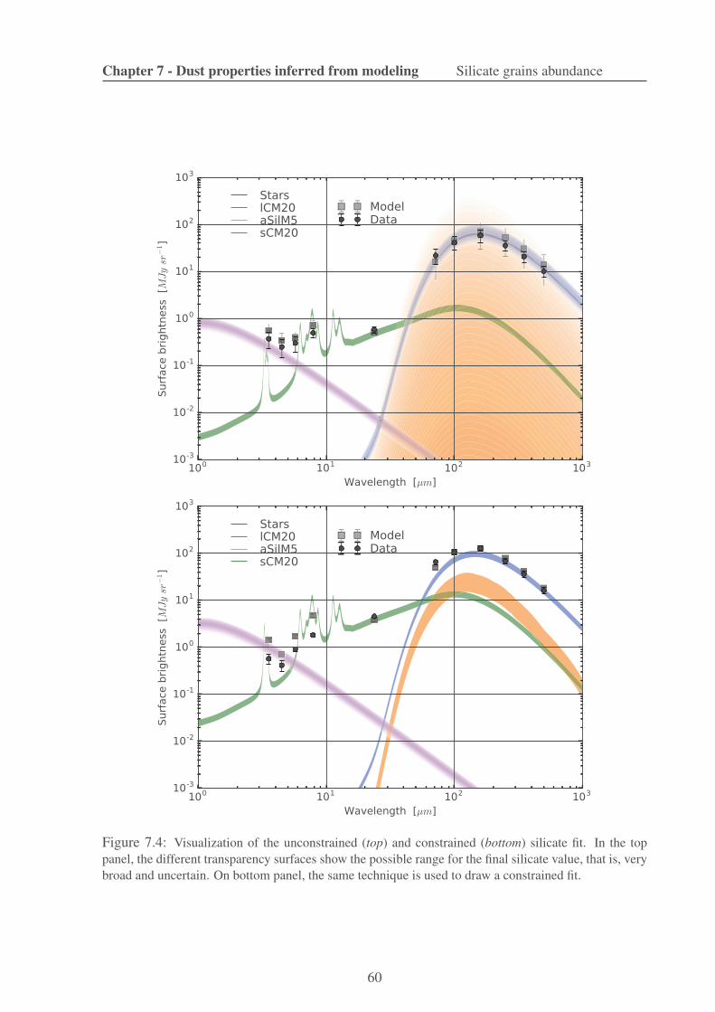
Chapter 7 - Dust properties inferred from modeling Silicate grains abundance
Figure 7.4: Visualization of the unconstrained (top) and constrained (bottom) silicate fit. In the toppanel, the different transparency surfaces show the possible range for the final silicate value, that is, verybroad and uncertain. On bottom panel, the same technique is used to draw a constrained fit.
60

Chapter 7 - Dust properties inferred from modeling Dust masses and gas-to-dustratios
7.3 Dust masses and gas-to-dust ratios
I computed total dust masses to assess whether or not the models produce reasonable amountsof dust in each case. I use multiple realizations of the likelihood in each pixel to estimatethe total dust mass uncertainty. Contrary to the maximum likelihood or the expectation value,the realization samples the likelihood and therefore takes into account the contribution that thefitting noise, for each pixel, makes to the uncertainty in the total dust mass.
I created 70 maps from the realizations; where the sum of every one of these maps gives atotal dust mass. The final total dust mass is the average of the realizations. Uncertainties on thisvalue are given by the distribution of the total dust masses. I derive the total dust mass frompixels that are detected in eight bands (see beginning of Section 6) of the fit, at a level of at least3σ above the background noise. This corresponds to a surface of ∼ 2.1×10⁶ pc2 (∼ 1.8°2) inthe SMC and ∼ 1.0× 10⁷ pc2 (∼ 14°2) in the LMC. The dust masses are given in Table 7.1;they range from ∼ 2.9 to 8.9×10⁴ M⊙ in the SMC and ∼ 3.7 to 4.2×10⁵ M⊙ in the LMC, forTHEMIS. I gather the results in the form of dust mass ± statistical uncertainty ± systematicuncertainty. The statistical uncertainty comes from the quality of the fits. It is very low due tothe number of constraints I have. The systematic uncertainty comes from our understanding ofthe models and their limitations. More precisely, I refer to the uncertainty on dust propertiessuch as emissivity (e.g., Weingartner & Draine 2001; Draine & Li 2007; Gordon et al. 2014),density, and the approach to building the optical and heating properties of dust grains (e.g., Mietheory, spherical grains). I also include degeneracies that come from the choices of ISRF (e.g.,a softer ISRF with more dust mass or a stronger ISRF with less dust mass).
Given the constraints on the requirement for a pixel to be fitted, there are a large numberof ‘undetected’ pixels. However, altogether, these regions may contribute significantly to thedust-mass estimation. In order to take these pixels into account, I average their emission ineach band to get an average SED. I fit this SED with the same models, and multiply by thesurface area of all the undetected pixels to obtain a total dust mass. In the SMC, including thecontribution from pixels below the detection threshold increases the dust masses given in Table7.1 from 50 to more than 100%, doubling the mass in some cases. This is due to the very sparsepixel detection in this galaxy. The ‘undetected’ area is approximately 10 times larger than thearea covered by pixels detected. In the LMC, the ‘undetected area’ is approximately the samesize as the fitted area and accounts for ∼ 10− 20% of the dust mass; H I mass, and GDR fordetected and undetected pixels are given in Table 7.1.
In Figure 7.5, I gather some of the dust masses found in the literature for the Magellanicclouds and this work. The dust masses I derived in this study are smaller than those estimatedby previous studies, especially for the simplest model. One interpretation of this difference liesin the carbon grains dominating this model fitting. The silicate emissivity is lower than that oflarge carbonaceous grains (∼ 5 cm2 g−1 and ∼ 17 cm2 g−1 at 250 µm, respectively). Therefore,for identical luminosity, if the fit uses only carbon grains, it requires less dust to produce thesame flux than if it used both carbon and silicates. Because the best results indicate a very smallcontribution of silicates, this eventually leads to a lower dust mass. The environment, throughthe definition of the ISRF, seems to have a strong impact on the dust masses. Although it ishard to evaluate a quantitative difference with residuals (Section 6), the final dust masses witha mixture of ISRF are closer to the values found in other studies.
I performed a test fit to verify this assumption: in THEMIS, I tied the large grain populations(aSilM5 + lCM20) together, using a single-ISRF approach. In this process, the informationregarding the independent distribution of the two types of grains is lost, but this resulted in dustmasses that are closer to those from Gordon et al. (2014), especially in the SMC; the LMC
61

Chapter 7 - Dust properties inferred from modeling Dust masses and gas-to-dustratios
Table 7.1: Dust masses and GDR in the SMC and the LMC.
Pixels > 3σ detection Including pixels < 3σ detection
Model Mdust [M⊙] GDR Mdust [M⊙] GDR
SMC
THEMIS single ISRF 2.86±0.005±0.8×10⁴ ∼ 4100 6.83±0.007±1.9×10⁴ ∼ 1750
THEMIS 2 ISRFs 8.93±0.04±2.5×10⁴ ∼ 1300 2.65±0.08±0.8×10⁵ ∼ 500
THEMIS multi-ISRFs 7.68±0.02±2.3×10⁴ ∼ 1500 1.20±0.07±0.3×10⁵ ∼ 1000
THEMIS αsCM20 free 6.25±0.01±1.7×10⁴ ∼ 1900 1.01±0.009±0.3×10⁵ ∼ 1200
MC11 3.44±0.006±1.0×10⁵ ∼ 350 3.71±0.006±1.1×10⁵ ∼ 910
LMC
THEMIS single ISRF 3.74±0.004±1.1×10⁵ ∼ 650 4.51±0.008±1.3×10⁵ ∼ 550
THEMIS 2 ISRFs 4.25±0.01±1.2×10⁵ ∼ 570 4.89±0.04±1.4×10⁵ ∼ 500
THEMIS multi-ISRFs 3.81±0.004±1.1×10⁵ ∼ 650 4.73±0.005±1.4×10⁵ ∼ 520
THEMIS αsCM20 free 4.21±0.005±1.3×10⁵ ∼ 580 4.88±0.008±1.4×10⁵ ∼ 500
MC11 2.05±0.001±0.6×10⁶ ∼ 120 2.11±0.002±0.6×10⁶ ∼ 170
Note: The total H masses in the SMC and the LMC are 1.2×10⁸ M⊙ and 3.3×10⁸ M⊙ for pixelsabove the 3σ detection, and 2.4×10⁸ M⊙ and 3.62×10⁸ M⊙ when accounting for pixels below the3σ detection.
being only slightly affected by the change. This seems to confirm the assumption that the lowdust mass I find comes from the carbon grain-dominated fitting results.
The gas-to-dust ratio (GDR) estimation of a galaxy varies depending on the approach. Fol-lowing Roman-Duval et al. (2014), I determined GDRs using H I measurements (Stanimirovicet al. 2000; Kim et al. 2003), and CO measurements (Mizuno et al. 2001) converted to H2 massestimations. The GDR estimations are thus really hydrogen-to-dust ratio, but, for clarity, I keepthe ‘GDR’ notation. I use the conversion coefficients XCO = 4.7× 1020 cm−2 (K km s−1)−1
from Hughes et al. (2010) for the LMC and XCO = 6× 1021 cm−2 (K km s−1)−1 from Leroyet al. (2007) for the SMC. I report values of GDR in Table 7.1. As mentioned above, the dustmasses with this model fitting are lower than the masses found by other works. This translatesto higher gas-to-dust ratios. Roman-Duval et al. (2014) found GDR of ∼ 1200 for the SMC and∼ 380 for the LMC, using dust surface density maps from Gordon et al. (2014). From Table7.1, the GDR values derived from the favored fits (two-ISRF and multi-ISRF models) rangefrom 1000 to 1200 in the SMC, and from 500 to 520 in the LMC. Using the model with tiedlarge grains, we find GDRs lower than those found by previous studies (∼ 700 in the SMC and∼ 400 in the LMC), and the shape of the observed SED is not well reproduced.
These GDRs show some variations (a factor of ∼ 2 in the SMC between the higher andlower values). In order to assess a stronger constraint on the GDR, I compare these results toindependent results given by depletion measurements or extinction.
Using the MW depletion patterns and the MCs abundances, one would expect GDRs of540-1300 in the SMC, and 150-360 in the LMC. This assumes a similar dust compositionand evolution between galaxies at different metalicities. I find values approximately 2 timeshigher than this. Tchernyshyov et al. (2015) used UV spectroscopy to derive depletions in theMCs. They found that scaling the MW abundances to lower metalicity, although approximately
62

Chapter 7 - Dust properties inferred from modeling Dust masses and gas-to-dustratios
Figure 7.5: Summary of the dust masses. Results from this work (right of the dashed line) are lowerthan previous studies. This likely comes from the low silicate abundances found in this paper.
correct in the LMC, can lead to significantly different numbers in the SMC than those derivedwith depletions. From their results, they predict a range of GDRs: 480-2100 in the SMC and190-565 in the LMC. My results fall within these limits. Their measurements were restricted tothe diffuse neutral medium (DNM). Since I cover the diffuse to dense parts of the galaxy, onewould expect more dust inferred from my fitting and thus, slightly lower GDRs.
Another way to predict GDR is to use extinction measurements. Gordon et al. (2003) mea-sured the dust extinction and H I absorption column in the SMC and LMC, deriving N(H I)/A(V)values. I determined the corresponding GDR expected from their results, using:
1/GDRSMC
1/GDRMW=
[N(H I)/A(V)]MW
[N(H I)/A(V)]SMC(7.1)
with DGRMW = 1/150. I used the averaged values in the SMC Bar, LMC, and LMC2 (super-shell) from their sample. I find reasonable values compared to their work.
Globally, my GDRs are in agreement with other studies that use different sets of measure-ments than IR emission. My fits manage to reproduce the observed SEDs and fall within reason-able ranges for dust masses and GDR. Previous studies have gathered GDR estimations fromnumerous programs and estimated a trend between the metalicities of galaxies and their gas-to-dust mass ratios (e.g., Engelbracht et al. 2008a,b; Galametz et al. 2011; Rémy-Ruyer et al.2014). I report my GDRs with the metalicity of the MCs (12+log(O/H) ∼ 8.0 in the SMC and∼ 8.3 in the LMC Russell & Dopita 1992) and found that the values are in agreement with thetrend.
63

Chapter 7 - Dust properties inferred from modeling Dust masses and gas-to-dustratios
64

8Exploring the impact of inferred dust
properties
8.1 Grain formation/destruction
Results from this first study on dust emission in the Magellanic Clouds indicate that the silicategrains are not found in the same amounts in the LMC and the SMC with respect to carbongrains. The fits show that the silicate/carbon ratio is unlikely the same in the MW, LMC, andSMC.
The lack of fully constrained fits of the silicate component suggests a deficit in silicate grainabundance, particularly in the SMC. This deficit could either be explained by less formation orby more destruction of silicate grains. Bocchio et al. (2014) showed that silicate grains are lesseasily destroyed than carbon grains in supernovae (SNe) due to their higher material density.This may therefore indicate that the higher abundance of carbon grains that I obtain is due tomore efficient carbon dust formation rather than selective silicate destruction. This could beconsistent with the low metalicity of this galaxy. It is well established that carbon stars formmore easily at low metalicity (e.g., Marigo et al. 2008). Nanni et al. (2013) showed that suchcarbon stars are efficient producers of carbonaceous dust. With the carbon excess, O-type dustis unlikely to form due to the absence of M-type stars. Recent work by Dell’Agli et al. (2015)investigated the evolution of AGB stars in the SMC using Spitzer observations. Using color-color diagrams built from photometry and modeling, they identify C-rich and O-rich stars atvarious masses. They found discrepancies between their distribution in the LMC and SMC.The amount of O-rich AGB stars in these samples is lower in the SMC than in the LMC, whichis ∼ 5%. This idea is in agreement with depletion studies (e.g., Welty et al. 2001; Tchernyshyovet al. 2015).
Yet, other studies have found constraints on the amount of silicates in the SMC. Weingartner& Draine (2001) constrained grain size distribution in the MW, LMC, and SMC from elementaldepletions and extinction curves. They adjust a functional form for each grain population (car-bonaceous and silicate). In the case of the SMC, they reproduced the extinction curve towardAzV398 from Gordon & Clayton (1998), in the SMC-bar. Their results indicate a larger amountof silicate dust than carbon dust. Their result is therefore opposite to ours. However, I did not
65

Chapter 8 - Exploring the impact of inferred dust properties Extinction curves
make observations of the same nature, nor did I use the same dust models. In the followingsub-section, I investigate the extinction curves in the MCs.
8.2 Extinction curves
Past programs measured extinction curves in the MCs, and have assessed discrepancies withthe extinction curves in the MW (steeper far-UV slope, absence of 2175 Åbump). Gordon et al.(2003) analyzed observed extinction curves in the MCs (5 in the SMC and 19 in the LMC)and derived RV values. In their sample, most of the curves could not be reproduced using therelationship based on MW extinction curves. They found 4 curves in the LMC (Sk -69 280, Sk-66 19, Sk -68 23, and Sk -69 108) that show a MW-like extinction curve.
The goal here is to verify if a fit of the dust emission in the MCs allows us to reconstruct theobserved extinction in the line of sight available. I did not try to directly fit the MCs extinctioncurves and the corresponding SED in emission at the same time. I extracted extinction curvesat the same positions indexed in Gordon et al. (2003) (4 in the SMC – I did not fit the pixelcorresponding to the AzV456 position, and all 19 in the LMC). Using the derived quantities foreach grain species from my fits, I calculated extinction curves with the DustEM outputs. I onlyderived extinction curves for the single-ISRF model and the model where αsCM20 is free. In themulti-ISRF model, the dust composition does not change when I compute the mixture spectra,therefore each extinction curve is the same and I do not use this variation to infer conclusions.
In the LMC, I reproduce the extinction observations in the four lines of sight that showeda MW-like shape. In the SMC, none of the extinction curves can be reproduced using the dustpopulation derived from IR emission fitting. This is also true for the rest of the LMC sample.In Figure 8.1, I show two results of extinction curves derived from the IR fitting (all curves areshown in Appendix A). I plot the observed and modeled extinctions in AzV -66 88 (LMC) inthe right panel. The αsCM20 = 5.4 is very close to the default value in the single-ISRF model.Given the similar abundance values, the modeled extinctions are therefore comparable. In theSMC (left panel, AzV 398) as well, αsCM20 = 5.4 and the result is close to that of a single-ISRF.In other lines of sight (e.g., AzV 214), a lower αsCM20 (e.g., ∼ 3) helps to match the near-IRpart of the observed extinction (1 6 λ−1 6 3). However, in both cases, the steep UV slope isnot well fit at all.
When the shape of the extinction curve is different from that of the MW, the dust propertiesinferred from IR emission correspond to an extinction curve that do not match that observed inthe UV. This could be due to the nature of dust grain models that are based on a MW calibration.It could also be due to a poor constraint on the small grain population by the IR emission,because the starlight and dust emission are mixed at those wavelengths. Either fitting the IRemission solely is not a good approach for deriving a quantitative impact of the small grainson the extinction, or the small grain population needs to be split in order to derive variousproperties that do not affect emission and extinction in the same way. This result accounts for thedifferences one may find when separately fitting the dust emission and extinction. Weingartner& Draine (2001) used one extinction curve in the SMC (toward Azv398) to constrain a sizedistribution. They found a larger amount of silicate than carbon. In the same line of sight,the result from fitting the emission reproduces the observed extinction. However, allowing fora larger amount of silicate than carbonaceous grains, as suggested by Weingartner & Draine(2001) results, does not help to match the IR observations.
66

Chapter 8 - Exploring the impact of inferred dust properties Extinction curves
Figure 8.1: Observed extinction curves (grey circles) in the LMC (right: Sk -68 129) and the SMC (left:AzV 398). I overplot the dust extinction derived from IR-emission fitting for a single-ISRF (dark redline) and a αsCM20 free model (purple line), and with smaller silicate grains (blue line, see Section 8.3.2).
67

Chapter 8 - Exploring the impact of inferred dust properties Other variations in dustmodels
8.3 Other variations in dust models
In this study, I investigated the change of model SED shape through variations in the ISRFenvironments, and by allowing independent grain variations. I showed that such changes sig-nificantly increase the quality of the fits, especially in the SMC. Those variations mainly affectthe 8−100 µm range by steepening the 8/24 µm slope and/or broadening the IR peak around100 µm. Other studies can provide more suggestions for changing the composition of dustmodels.
8.3.1 Change in carbon size distribution
Köhler et al. (2015) studied the dust properties evolution from diffuse to dense regions. Forexample, they showed that grains with an additional mantle have different properties that canlead to a steepening of the FIR slope and a lower temperature. They also investigated theinfluence of forming aggregates in dense media. In that case as well, the dust properties varysignificantly. Such approaches could be helpful for fitting the MCs dust emission. In Figures6.2 to 6.4, we can see THEMIS is slightly above the observations in the FIR (at 250, 350, and500 µm). A steepening of the spectral index may suggest that the model would better match thedata at these wavelengths.
Ysard et al. (2015) also investigated the variations of dust properties observed with Planck-HFI. In their study, they investigated the impact of varying the carbon abundance, while keepingthe silicate abundance constant. They found that this variation could help reproduce the obser-vation and account for the dust variations. They showed that changing the size distribution (bychanging the aromatic-mantle thickness or the size distribution function) participates in the dustvariations. This provides additional evidence that a single model with fixed size distribution isnot appropriate for fitting observations on a galaxy scale.
8.3.2 Allowing smaller silicate grains
Bocchio et al. (2014) computed size distribution, emission, and extinction curves for carbona-ceous and silicate grains from THEMIS in environments where dust is destroyed/sputtered byshocks with v ∼ 50−200 km/s. At sufficiently high shock velocities, carbon grains are mostlydestroyed, whilst silicates are fragmented into smaller grains due to their collisions with smallcarbon grains. Using their silicate grain size distribution leads to a steepening of the far-UV ex-tinction. Looking at the peculiar shape of the SMC extinction, this approach seems interesting.Once again, I want to know if fitting the dust emission can yield a good estimation of the dustextinction.
Allowing for smaller silicate grains helps to match the data in the IRAC bands, in the SMC.In the LMC, on the other hand, the residuals are not affected significantly, and the fits are notimproved. However, in both galaxies, we notice a change in the extinction shape. The far-UVslope is closer to the observations. In Figure 8.1, the cyan-dashed lines are those derived for afit of the emission with smaller silicate grains. In the SMC, two lines of sight are significantlyimproved by the change in the silicate size distribution. My results still exhibit a small bumparound 2175 Å, because I allow the small carbonaceous grains to vary. In the LMC, some linesof sight are greatly affected and the extinction can be matched with smaller silicates; see, forexample, the left panel of Figure 8.1.
I only applied the new size distribution to a single-ISRF environment to test the resulting ex-tinction with DustEM. In terms of dust masses, the new fits lead to ∼ 4.4×10⁴ M⊙ in the SMC,
68

Chapter 8 - Exploring the impact of inferred dust properties Impact of the ISRFshape
and ∼ 2.0×10⁵ M⊙ in the LMC, respectively higher and lower than a single-ISRF environment,without the change in size distribution.
8.3.3 On the recalibration
In this study, I used a different reference SED to rigorously compare models after they wererecalibrated on the same Galactic values. However, it should be noted that the models arenot defined as such. In THEMIS, the GDR is set to approximately 134 (Ysard et al. 2015).Without recalibration, I would obtain a dust mass of ∼ (1.9−5.6)×104 M⊙ in the SMC, and∼ (2.3−2.7)×105 M⊙ in the LMC, for the different variations of environment. THEMIS massdistribution for the grain populations is different than in other dust models (e.g., Draine & Li2007). For example, the silicate (pyroxene and olivine type) grains have a lower specific massdensity. Therefore, the model needs less silicate mass. We can also notice that the carbon massis mostly found in small carbonaceous grains.
In order to get a more accurate mass estimation, one possible path of investigation is to usethe different versions of the model to fit the various media of a galaxy, namely dense or diffuse.In THEMIS, dust in the transition from the diffuse ISM toward dense molecular clouds is de-scribed with aSilM5 and lCM20 grains coated with an additional H-rich carbon mantle. Insidedense molecular clouds, further evolution is assumed and THEMIS dust consists of aggregates(with or without ice mantles).
All methods and results up till this section have been publish in Chastenet et al. (2017). Iexplored other leads after publication, that I describe here.
8.4 Impact of the ISRF shape
As we have seen in the Introduction, the dust emission is dependent on the surrounding energyprovided by stars, which is modeled as the ISRF. Thanks to the design of the DustEM tool, it ispossible to directly change the ISRF shape, in addition to changing its intensity with a scalingfactor. The work of Mezger et al. (1982) and Mathis et al. (1983), presented in Section 1.3 of theIntroduction part, has determined the shapes of ISRF at various distances DG from the Galacticcenter. Their studies provide us with ISRF at DG =5, 6, 8, 10 and 13 kpc. Although the ISRFat DG = 10 kpc is the most used, there is no a priori reason to think that a single ISRF shapeis a realistic choice to model dust emission in galaxies. Their star formation rates, ages or thedistribution of dust are not unique, and they all directly affect the ISRF. Adapting the predicteddust emission in our model based on a different estimations of starlight energies seems to be areasonable approach.
I fit the same data sets using THEMIS, in environments recreating different ISRF hardness.To do so, I implemented the ISRF from Mezger et al. (1982) and Mathis et al. (1983) at allgalacic radii (not just the solar neighborhood), into the right format for DustEM., allowing meto derive new dust emission spectra. I then built a library of dust models following the approachpresented in Section 6.1. The goal was to let the fit choose between different shapes of ISRF aswell as its intensity.
The maps showing the type of ISRF chosen are displayed in Figure 8.2. The first strikingdifference is the average ISRF value in each galaxy. In the SMC, a hard ISRF at DG = 5 kpc(dark blue in Figure 8.2) apparently fits well the data, while a softer ISRF at DG = 13 kpc (darkred in Figure 8.2) is mostly chosen in the LMC. We know the two galaxies are not at the samestage of star formation, and we can therefore suspect the global energy absorbed by dust would
69

Chapter 8 - Exploring the impact of inferred dust properties Impact of the ISRFshape
Figure 8.2: Values of the ISRF distance DG from a fit allowing for various ISRF shapes, in the SMC(top) and the LMC (bottom). The two galaxies show striking differences: the LMC is better fit with asoft ISRF while the SMC shows the hardest value.
70

Chapter 8 - Exploring the impact of inferred dust properties Using Draine & Li(2007)
not be identical. This could be the reason of this difference of preferred ISRF shape betweenthe MCs.
However, we can also notice the spatial variations within each galaxy. This is most visible inthe LMC, where harder ISRF seems to be better to fit dust emission in brighter regions. Theseregions, in blue in the right panel of Figure 8.2, appear to be located at the same position asHII regions, where ionized gas is present. The same behavior was noticeable with the αsCM20parameter in Section 6.3. Once again, it indicates that the shape of the dust emission is not thesame in these regions, requiring a change in predicting the emission spectrum. In the SMC, itlooks like the H II regions also show a different result than the rest of the galaxy, but in a moreunexpected way. In these regions, where the energy heating dust should be greater, the fit showsthat a softer ISRF is better at reproducing the data. It is surprising, and not understood at thistime, but further investigations could bring more insights on this result.
Nonetheless, this approach is interesting as it shows that not all galaxies behave the sameway in terms of preferred shape of ISRF. It means that, as suspected, a single ISRF is notnecessarily sufficient to accurately reproduce dust emission in other galaxies. At the very least,it depicts a need to change the predicted dust emission spectrum, in a way or another.
8.5 Using Draine & Li (2007)
I fit the Magellanic Clouds dust emission with the DL07 model. I used the MW-based model,and not the size distributions that were based on MCs observations in Weingartner & Draine(2001). Further use of these models has shown that they were not able to fit the MCs themselves.
The D07 model does not provide a significantly better fit to the Magellanic Clouds thanTHEMIS overall. On Figure 8.3, I show the residuals for the SMC (left) and the LMC (right).
Figure 8.4 shows the parameter maps in the SMC (top), and the LMC (bottom). We cannotice some difference in the values of the parameters, which vary between both galaxies. Forinstance, the qPAH value in the SMC appears to be on average smaller than in the LMC. In theformer, the average value for qPAH is around 1%, while in the latter, it is 4%. It is consistentwith the Draine et al. (2007) results on qPAH as a function of metallicity. It may indicate adifference in dust evolution, either in PAH formation or their destruction. It is possible that astronger radiation field sputters the PAH, reducing their abundance. In both galaxies, we do notobserve a significant value of qPAH at high Umin. The β value (power-law coefficient for ISRFintegration in the DL07 model (see Section 12.2.1), also seems slightly higher in the LMC thanin the SMC, on average. A higher β translates into more weight of the small U in the integration.In the LMC, we can see a relation between this parameter and γ (the relative weight of the dustmixture at various temperatures, and the dust heated at a single temperature). In regions whereβ is high, i.e. with more impact of the small U , the best fit chooses a small γ , i.e. putting all theweight on the dust heated at a single temperature. This could be interpreted as, in each pixel,a single bright star dominates the dust heating and can be modeled without requiring multiplesources. This opposition is not as visually striking in the SMC, and does not seem to happen.
71

Chapter 8 - Exploring the impact of inferred dust properties Using Draine & Li(2007)
Figure 8.3: Histograms of fractional residuals for DL07 (brown bars) in the SMC (top) and the LMC(bottom). For reference, THEMIS in a single ISRF is shown by red bars.
72

Chapter 8 - Exploring the impact of inferred dust properties Using Draine & Li(2007)
Figure 8.4: Parameter maps of the Magellanic Clouds fit with the DL07 model. Striking differencesappear between the SMC and the LMC.
73
Chapter 8 - Exploring the impact of inferred dust properties Using Draine & Li(2007)
74

9Conclusions and perspectives on dust in the
Magellanic Clouds
I fitted the Spitzer SAGE and Herschel HERITAGE observations of the Magellanic clouds at∼ 10 pc, in 11 bands from 3.6 to 500 µm. I used three physical dust grain models: Compiègneet al. (2011), THEMIS (Jones et al. 2013; Köhler et al. 2015) and Draine & Li (2007) to modeldust emission in the IR.
Globally, I find that the Compiègne et al. (2011) model should not be used in this contextas it suffers from strong discrepancies with respect to the observations (e.g., large-grain steepemissivity in the FIR). Fitting THEMIS on the observations gives better residuals, especiallyin the SMC. THEMIS leaves a small deficit in the residuals in the FIR, that is, it is too lowcompared to the observations, in opposition to what has been identified in previous studies atan excess at 500 µm. I find that using more than a single ISRF greatly improves the qualityof the fit. More generally, a change in the shape of the model SED will help to get betterresiduals, either by using more than a single-ISRF environment, or by changing the dust grainsize distribution, with respect to the one calibrated on the diffuse ISM in the solar neighborhood.Parameter maps depict very model-dependent spatial variations. The approach chosen for thedust environment (ISRF) strongly affects the quality and result of the fits.
Using the THEMIS dust model, I find that the silicate abundance is estimated only as anupper-limit YaSilM5 ∼ 100.4MaSilM5
⊙ /MH, while the large carbonaceous grain emission is con-strained with well defined peaked likelihood distributions. The silicate/carbon ratio implied bythe fits indicates an evolution between the MW and the MCs. This ratio is approximately 10 inthe MW, but is not the same or constant throughout the MCs (6 1 in the SMC and LMC). Testsforcing a MW-like silicate/carbon ratio lead to very broad residuals and poor fitting, confirmingthat this ratio should not be kept constant for these galaxies.
The dust masses derived in the LMC from my fitting are lower than those derived by otherstudies by a factor lower than two, but remain close given the uncertainties (of ∼ 30% total).In the SMC, the values are in agreement with the literature (e.g., Gordon et al. 2014) but sufferfrom large uncertainties. The numerous pixels with the low upper-limit on silicate abundanceare mostly responsible for the slightly lower dust masses (especially in the SMC), because thecarbonaceous grains have a lower mass.
75

Chapter 9 - Conclusions and perspectives on dust in the Magellanic Clouds
I used the dust emission results to create modeled extinction curves. I find that fitting onlythe emission cannot give results that can be applied directly to match the measured dust ex-tinction in the MCs. These tests showed that a change in the estimated grain size distributions(based on MW measurements) would be needed to (more) accurately match the MCs extinctionfrom an emission fitting (e.g., different silicate grain distribution, namely smaller).
Further work will use additional dust grain models for comparison (e.g., Draine & Li 2007,THEMIS with aggregates), while the goal should remain the same, that is, to compare dustemission/extinction results from various dust models using a strictly identical fitting technique.In order to fully interpret these data, a more detailed approach, for example taking into accountthe gas-phase transitions, is needed (but is beyond the scope of this paper). A radiative transfertechnique should also be used to understand the errors of the assumptions made when devel-oping a dust model. The simplest heating environment ‘single-U’ is unlikely to be enough tofit dust emission in nearby galaxies, and the more sophisticated one (‘multi-U’) is empiricallychosen. A more realistic approach, compared to the more simple descriptions, could be helpfulin improving dust emission fitting techniques.
Linking the emission and the extinction was only briefly mentioned in this thesis. Anotherapproach to what we have seen would be to directly fit the emission and the extinction at thesame time. This is not an easy step, but could provide important clues on the connections be-tween dust properties that can be seen in emission and those that can be seen in extinction.Can both observables be adjusted correctly with our current models? Or can we fit them wellonly separately? If the ISRF hardness and intensity can be constrained with the emission, whatvariations does that allow in extinction? Extinction curves can show strong differences from aline-of-sight to the next: how does that affect the fit in emission? Can we see strong differencein the dust properties in those cases?Even though polarization was not used in this work, it is another dust property that can beobserved. A recent appeal to this characteristic is becoming more and more important in duststudies, in particular with the availability of the Planck data. Dust grain alignment with the mag-netic field is a clue to its composition properties, and its surroundings. It is another observablethat could be linked with extinction and emission.
76

Chapter 9 - Conclusions and perspectives on dust in the Magellanic Clouds
PART II − TAKE AWAY
The results in this second part have been published in Chastenet et al. (2017). We wantedto fit the dust emission in two nearby galaxies with different full dust models, using aconsistent fitting technique.
What did we show:
• although they fit the MW diffuse ISM emission, all dust models are not equal whenit comes to fitting IR emission of other galaxies. Dust characteristics like the FIRslope is critical in that matter, and THEMIS appears to give better results.
• In terms of dust masses, THEMIS agrees within the errors with results in the liter-ature. Choosing a less well-fitting model to fit the IR emission leads to a differenceof an order of magnitude in dust masses.
• The spatial variations of derived parameters are sensitive to the choice of dust heat-ing environment. Considering a single-temperature dust or dust elements heated atvarious temperature impacts the results.
• Within the Magellanic Clouds and from a galaxy to the other, avarying Silicate/Carbonaceous grains ratio implies that dust composition isnot the same as in the MW. Although the Silicate abundance is estimated with anupper limit, the MW reference value for this ratio is rarely found.
• Dust extinction curves from emission properties in the Magellanic Clouds donot match the observations. However, variations in size distributions seem to bepromising.
• Studying the impact of the ISRF shape on dust emission fitting appears to bring in-teresting conclusions, showing striking differences from a galaxy to another.
That last remark will be our starting point for the next part. We will investigate the impor-tance of a better estimation of the dust heating environment, compared to the approacheswe have used in this part.
77

Chapter 9 - Conclusions and perspectives on dust in the Magellanic Clouds
78

Part III
Systematics in Dust Modeling
79


10Using radiative transfer in dust studies
The next part of this thesis focuses on using a more sophisticated and less empirical approach tomodel the dust heating. As we have seen in the previous parts, dust observables, and thereforethe properties that we derive, are highly dependent on the surrounding radiation field, and hencethe photons that dust grains can absorb, or scatter. Not only the intensity of the radiation field,i.e. the number of photons available, is an important factor, but also their energy hν will stronglychange the shape of the spectrum of the resulting dust emission. Moreover, highly energetic UVphotons can sputter small dust grains, and generate a new grain size distribution, rendering ourdust models inaccurate. To take into account the mixing effects, we use an empirical power-law of the ISRFs, to mix dust elements at various temperatures. However, we do not know forsure the limitations of that assumption. Moreover, in this case, only the intensity of the ISRFchanges, and not its shape. Knowing the radiation field at different positions in a cloud withthe best accuracy possible is of great importance to model dust. Thanks to the improvements incomputer technologies, speed and storage space capacities have rapidly increased, allowing forfast and long computations, necessary for radiative transfer calculations.
10.1 The Radiative Transfer method
The dust radiative transfer (RT) aims at understanding the transport of radiation in a more orless dusty medium. Like we have seen in the Introduction, the interstellar radiation field (ISRF)is defined by its intensity (number of photons) and hardness (energy of the photons). Solvingthe RT problem means determining the intensity of the radiation field in every position, inall directions, for each wavelength. This leads to greatly increasing the dimensionality of theproblem. Dust RT is therefore not a simple thing to do: it is a non-linear and non-local process,and modelers, facing numerous difficulties, are often forced to make assumptions to speed upthe calculations. The non-locality happens in the three dimensions: position, direction andwavelengths, making the simplifications very difficult. The RT approach has however becomea major problem to tackle in modern astrophysics, since technologies now allow investigatingit to some level of details, and because dust remains an –almost– omnipresent component ofthe universe. It is therefore a critical issue to solve. While observations show structures andcomplex 3D layouts, the simple (non-RT) approach is unable to convey such intricacy. The
81

Chapter 10 - Using radiative transfer in dust studies The Radiative Transfer Equation
source anisotropy also fails at being recovered if not done with a full 3D geometry. That iswhy more extensive studies focus on estimating the ISRF in a geometry, and that is why I aminterested in using this approach for this study. Using the realistic calculations brought by theRT model, and comparing it to the more simple approach in dust models will allow us to foreseethe limitations of our models.
10.2 The Radiative Transfer Equation
The complete radiative transfer equation (RTE) is a 6D integro-differential equation that in-cludes the integral for scattered light and a non-linear coupling between the thermal sourceterm and a double-integral equation. Moreover, the changing nature of the RTE, depending onthe varying extinction, makes it very difficult to input into solvers, and is inherently limited byresources, sometimes implying a limitation in the problem itself. We will go over some of thedetails of the RTE, from a simple form to a more complete expression, and the refinements thatcan be input.
Solving the RTE means determining the specific intensity I(xxx,nnn,λ ) of the radiation field,i.e. the amount of energy in a wavelength interval1; xxx represents the position vector, nnn, thedirection, and λ the wavelength. The general form of the RTE can be written:
nnn ·∇∇∇I(xxx,nnn,λ ) =−κ(xxx,λ ) ρ(xxx) I(xxx,nnn,λ )+ j(xxx,nnn,λ ) (10.1)
The left hand term describes the specific intensity variation on an infinitesimal distance. Thevariations are due to interactions with sinks, i.e. a decrease in the intensity: the first term on theright-hand side of the equation (equivalent to absorption), where κ is the the mass extinctioncoefficient, and ρ the mass density of the medium; or source terms: j, that describe a gain inintensity (due to stars, dust...). The complexity of the RTE depends on the nature of the previousterms (e.g. scattering, dust emission, starlight, absorption...).
It is possible to express the equation in terms of a physical distance s, at position xxx, andin direction nnn. Doing so, and assuming that j does not depend on the intensity I, there is ananalytic solution to the general form of the Equation 10.1:
I(s,λ ) =∫ s
−∞j(s′,λ ) e−τ(s,s′,λ ) ds′ (10.2)
with the optical depth τ beingdτ
ds= κ(s,λ ) ρ(λ ) (10.3)
In this specific case, it shows that the intensity depends on every position anterior to s.A physical description of Equation 10.1 is to take into account the primary emission, and
the absorption. In that case, the source term becomes j∗(xxx,nnn,λ ), describing a stellar componentadding energy to the radiative transfer. The extinction coefficient is therefore the dust absorptioncoefficient κabs(xxx,nnn,λ ). Although this case is still simple to solve, it leaves a complex part outof the radiative transfer, that unfortunately greatly complicates the problem: scattering.
1It can be determined in a frequency interval as well. For notation purposes, we will not use the Iλ (xxx,nnn,λ )notation, and will get rid of the subscript.
82

Chapter 10 - Using radiative transfer in dust studies The Radiative Transfer Equation
Scattering As explained in the Introduction, scattering is the redirection of the photon inanother direction. It is, however, quite complex: the direction in which the photon bouncesback is determine by a probability law Φ which depends on dust properties. It is therefore ananisotropic process, and changes the RTE as such:
nnn ·∇∇∇I(xxx,nnn,λ ) =−κabs(xxx,λ ) ρ(xxx) I(xxx,nnn,λ )
+ j∗(xxx,nnn,λ )
+κsca(xxx,λ ) ρ(xxx)∫
4πΦ(nnn,nnn′′′,xxx,λ ) I(xxx,nnn′′′,λ ) dΩ′
(10.4)
where κabs and κsca are the absorption and scattering coefficients, respectively. The newdirection nnn′′′ of a photon is given by the scattering phase function Φ(nnn,nnn′′′,xxx,λ ), that describesthe probability that a photon moving in direction nnn will have a new direction nnn′′′.
The complete RTE equation is quite complex, and some levels of refinement can be imple-mented but may be less important in some situations. If scattering is inevitable, modelers candecide how much physical input they want to add in the numerical solver. In the following arebriefly shown a few of them.
• Dust mixtures A dust model, even a simple one, usually describes dust as a mixtureof several components, with different chemistry (Section 2.6: carbonaceous and silicategrains), optical properties... To take this variety of properties into account, the RTE caninclude a sum of terms that translate the presence of multiple extinction coefficients; eachκ term in Equation 10.4 is therefore replaced with a sum:
−κext(xxx,λ )→−∑i
wi(xxx) κext,i(λ )
κsca(xxx,λ )→ ∑i
wi(xxx) κsca,i(λ )(10.5)
The wi(xxx) terms describe the contribution of each grain population to the total dust model.
• Adding dust emission Dust absorbs optical/UV light and re-emits the absorbed energyin the infrared. This emission can be included in the RTE with an additional sourceterm jd(xxx,λ ). As seen in Section 2.3, dust grains can be either in thermal equilibrium orstochastic heating. In the first case, the new source term can be written:
jd(xxx,λ ) = ∑i
wi(xxx) κabs,i(λ ) ρ(xxx) B(Ti(xxx),λ ) (10.6)
where B(Ti(xxx),λ ) is the Planck function, determined as a function of temperature andwavelength. In the case of stochastic heating, the source term is:
jd(xxx,λ ) = ∑i
wi(xxx) κabs,i(λ ) ρ(xxx)
[
∫ ∞
0Pi(T,xxx) B(T,λ ) dT
]
(10.7)
• Polarization Dust grains can polarize light. The scattering process leads to polarizedphotons. In the RTE, it is possible to take this phenomenon into account. If so, we do notsolve for the intensity I but for a vector SSS. The scattering term in Equation 10.4 becomesan integral including a matrix which describes the vector SSS.
In the end, one is free to choose the terms to input in the RTE to solve, depending on the amountof resources available and the physical requirements for the chosen situation. Once the RTE isconstructed, a technique to solve it must be implemented.
83
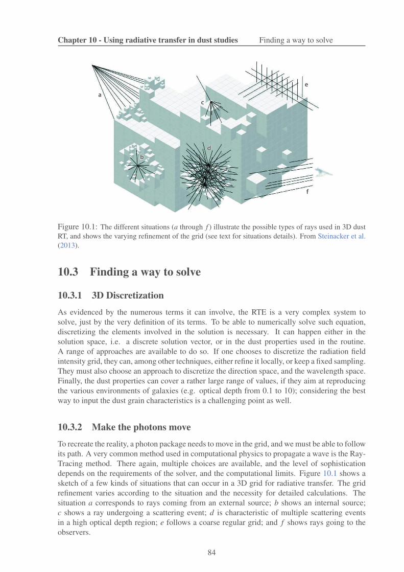
Chapter 10 - Using radiative transfer in dust studies Finding a way to solve
a
b
c
d
e
f
Figure 10.1: The different situations (a through f ) illustrate the possible types of rays used in 3D dustRT, and shows the varying refinement of the grid (see text for situations details). From Steinacker et al.(2013).
10.3 Finding a way to solve
10.3.1 3D Discretization
As evidenced by the numerous terms it can involve, the RTE is a very complex system tosolve, just by the very definition of its terms. To be able to numerically solve such equation,discretizing the elements involved in the solution is necessary. It can happen either in thesolution space, i.e. a discrete solution vector, or in the dust properties used in the routine.A range of approaches are available to do so. If one chooses to discretize the radiation fieldintensity grid, they can, among other techniques, either refine it locally, or keep a fixed sampling.They must also choose an approach to discretize the direction space, and the wavelength space.Finally, the dust properties can cover a rather large range of values, if they aim at reproducingthe various environments of galaxies (e.g. optical depth from 0.1 to 10); considering the bestway to input the dust grain characteristics is a challenging point as well.
10.3.2 Make the photons move
To recreate the reality, a photon package needs to move in the grid, and we must be able to followits path. A very common method used in computational physics to propagate a wave is the Ray-Tracing method. There again, multiple choices are available, and the level of sophisticationdepends on the requirements of the solver, and the computational limits. Figure 10.1 shows asketch of a few kinds of situations that can occur in a 3D grid for radiative transfer. The gridrefinement varies according to the situation and the necessity for detailed calculations. Thesituation a corresponds to rays coming from an external source; b shows an internal source;c shows a ray undergoing a scattering event; d is characteristic of multiple scattering eventsin a high optical depth region; e follows a coarse regular grid; and f shows rays going to theobservers.
84

Chapter 10 - Using radiative transfer in dust studies Finding a way to solve
10.3.3 Monte Carlo solution
Finally, the solving method needs to be implemented as well. The Monte Carlo (MC) methodhas been used for a long time in a large number of applications, in various areas, not restrictedto physics. Interesting and extensive overviews about MC methods in general, from Whitney(2011) or Steinacker et al. (2013), to name only a few, can be found. For astrophysics pur-poses, MC methods applied to transport of particles like photons, neutrons or cosmic rays haveemerged decades ago (e.g. Mattila 1970; Witt & Stephens 1974). The basic idea in MC is touse random numbers. In the case of RT, this applies to the path of a photon package: alongits journey, at each iteration, the new path of the photon package will be determined by ran-domly sampling a probability distribution function. Essentially, it means that instead of tryingto directly solve the RTE previously seen, the MC method treats it in a probabilistic approach.There is therefore a need to generate those random numbers, through an appropriate method.There are multiple ways to do so, and we will review only a few in the following. In bothcases presented, the solution emerges after numerous iterations. Each iteration corresponds toa movement of the photons packages. Each package is tracked until it is completely absorbs bydust grains, or until it escapes the grid.
Simple MC
If the dust emission is not used, the simple MC method can be done independently at eachwavelength (and therefore can be parallelized).
• The first step is the creation of the photon package, and its input into the computation. Itis created according to the source term j∗(xxx,nnn,λ ), and is assigned random position anddirection through the respective probability distribution functions.
• The next step is to determine the free path length, or how far the photon package cantravel without interacting with a sink/source term. To do so, it uses the optical depth τ ,which can be translated into a “physical” distance.
• At the new position, the photon is either absorbed or scattered by a dust grain, and theprobability distribution, now discrete, is set by the albedo of the grain κsca/κext. In thecase of an absorption event, it ends the package path. If the photon is scattered, a newdirection nnn′′′ is determined, and it goes back to the previous step. The repetition and thesecond and third steps goes on until there are no photons left in the computation space.
In the case of high optical depths, the grain density is high and absorption is more likely tooccur than scattering; these situations may induce errors due to the lack of iterations. To com-pensate, a minimum number of scattering events can be required, and ensure that the calculationis done for a sufficient number of times.
Weighted MC
Although practical, the simple MC method is only valid in 1D and 2D situations, thanks to themultiple symmetries that help to simplify the problem. In the case of 3D RT, such simplifica-tions cannot be made, and one is often required to use acceleration methods. One of them is theweighted MC method, or biasing. It is widely used. The basic idea is to use a different proba-bility distribution instead of the initial one, and then correct it after sampling. The correction ismade through a weight, assigned to the photon package, and varies depending on the accelera-tion method chosen. The recent work from Baes et al. (2016) has focused on this method in this
85
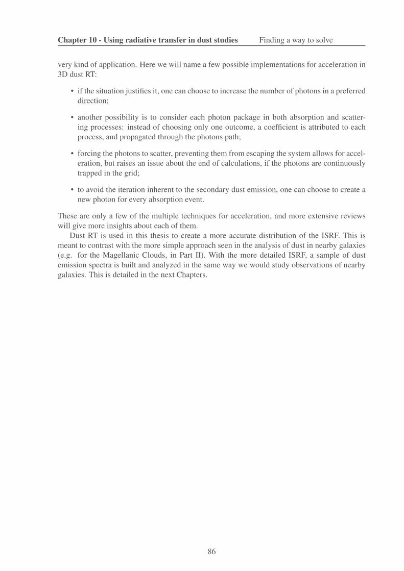
Chapter 10 - Using radiative transfer in dust studies Finding a way to solve
very kind of application. Here we will name a few possible implementations for acceleration in3D dust RT:
• if the situation justifies it, one can choose to increase the number of photons in a preferreddirection;
• another possibility is to consider each photon package in both absorption and scatter-ing processes: instead of choosing only one outcome, a coefficient is attributed to eachprocess, and propagated through the photons path;
• forcing the photons to scatter, preventing them from escaping the system allows for accel-eration, but raises an issue about the end of calculations, if the photons are continuouslytrapped in the grid;
• to avoid the iteration inherent to the secondary dust emission, one can choose to create anew photon for every absorption event.
These are only a few of the multiple techniques for acceleration, and more extensive reviewswill give more insights about each of them.
Dust RT is used in this thesis to create a more accurate distribution of the ISRF. This ismeant to contrast with the more simple approach seen in the analysis of dust in nearby galaxies(e.g. for the Magellanic Clouds, in Part II). With the more detailed ISRF, a sample of dustemission spectra is built and analyzed in the same way we would study observations of nearbygalaxies. This is detailed in the next Chapters.
86

11The DIRTYGrid
The RT calculations used for this thesis come from the RT code DIRTY (Gordon et al. 2001;Misselt et al. 2001). Using this RT routine and a dust emission calculator, Law et al. (inprep.) created the DIRTYGrid. This grid provides us with fluxes of dust emission in a numberof various environments, re-creating the diverse conditions in nearby galaxies.
11.1 DIRTYGrid description
The DIRTYGrid (Law et al., in prep.) uses the DIRTY code and the ISRF determined in eachcell to compute the corresponding SED at each position of the grid. Figure 11.1 shows a blockdiagram of the two routines used to creates the DIRTYGrid. The wavelength range extends fromthe UV to the submillimeter. Here, we review some important points of this work, crucial to thefollowing study.
The parameters in the DIRTYGrid are meant to cover a large range of galactic properties, asseen in numerous observations. There are seven free parameters in the DIRTYGrid. Three ofthem are ‘discrete’:
• grain type: there are three possible choices of grain composition, coming from those usedin Weingartner & Draine (2001).
– The first is a Milky-Way-type dust, based on MW abundances, emission and extinc-tion. Weingartner & Draine (2001) offer different possibilities of such composition,and that in the DIRTYGrid is for RV = 3.1, and bC = 6×10⁵ (number of C atoms).
– The second choice is a LMC-type dust, based on constraints from the super-shelllocated south-east of 30 Dor1. In this case, bC = 6×10⁵.
– Finally, the last choice is an SMC-type grain composition, based on constraints inthe SMC Bar (the main structure of the galaxy, see Figure 4.1).
130 Doradus is the brightest star formation region in the LMC. It is extensively studied for its stellar propertiesas well as its dust characteristics.
87
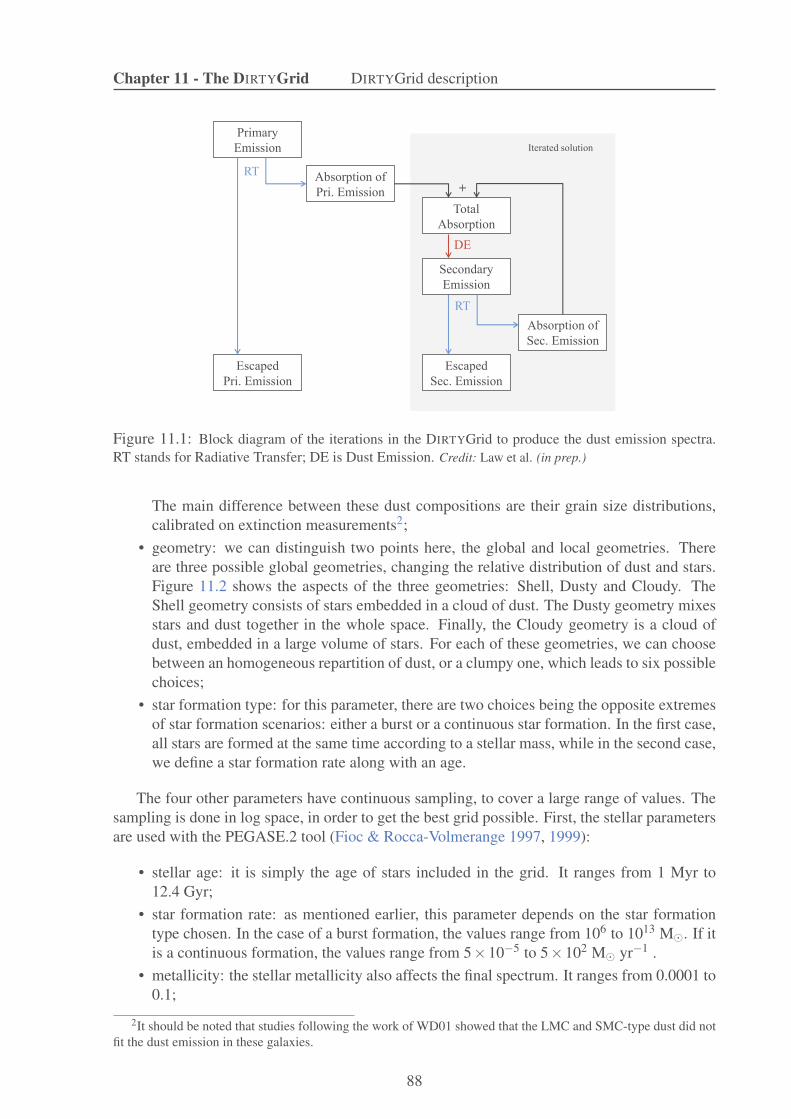
Chapter 11 - The DIRTYGrid DIRTYGrid description
Primary
Emission
Escaped
Pri. Emission
Absorption of
Pri. Emission
Total
Absorption
Secondary
Emission
Escaped
Sec. Emission
Absorption of
Sec. Emission
RT
RT
DE
+
Iterated solution
Figure 11.1: Block diagram of the iterations in the DIRTYGrid to produce the dust emission spectra.RT stands for Radiative Transfer; DE is Dust Emission. Credit: Law et al. (in prep.)
The main difference between these dust compositions are their grain size distributions,calibrated on extinction measurements2;
• geometry: we can distinguish two points here, the global and local geometries. Thereare three possible global geometries, changing the relative distribution of dust and stars.Figure 11.2 shows the aspects of the three geometries: Shell, Dusty and Cloudy. TheShell geometry consists of stars embedded in a cloud of dust. The Dusty geometry mixesstars and dust together in the whole space. Finally, the Cloudy geometry is a cloud ofdust, embedded in a large volume of stars. For each of these geometries, we can choosebetween an homogeneous repartition of dust, or a clumpy one, which leads to six possiblechoices;
• star formation type: for this parameter, there are two choices being the opposite extremesof star formation scenarios: either a burst or a continuous star formation. In the first case,all stars are formed at the same time according to a stellar mass, while in the second case,we define a star formation rate along with an age.
The four other parameters have continuous sampling, to cover a large range of values. Thesampling is done in log space, in order to get the best grid possible. First, the stellar parametersare used with the PEGASE.2 tool (Fioc & Rocca-Volmerange 1997, 1999):
• stellar age: it is simply the age of stars included in the grid. It ranges from 1 Myr to12.4 Gyr;
• star formation rate: as mentioned earlier, this parameter depends on the star formationtype chosen. In the case of a burst formation, the values range from 106 to 1013 M⊙. If itis a continuous formation, the values range from 5×10⁻⁵ to 5×10² M⊙ yr−1 .
• metallicity: the stellar metallicity also affects the final spectrum. It ranges from 0.0001 to0.1;
2It should be noted that studies following the work of WD01 showed that the LMC and SMC-type dust did notfit the dust emission in these galaxies.
88

Chapter 11 - The DIRTYGrid Public distribution
Shell Dusty Cloudy
Figure 11.2: 3D representations of the geometries used in DIRTYGrid. Left to right: Shell has a core ofstars surrounded by dust, Dusty is a mixture of stars and dust, Cloudy has a core of dust surrounded bystars.
Finally, there is a last free parameter in the DIRTYGrid:
• optical depth: this parameter, τV, translates the amount of dust, and ranges from 0.1 to10.
Outputs
The final output of the DIRTYGrid is a spectrum, for each parameter set detailed above. Thisspectrum has been integrated in a large number of photometric bands (e.g. GALEX, Spitzer,Herschel, ...) and these synthetic SEDs are the product I am using for this study. Figure 11.3shows examples of spectra displaying variations in each parameter space. These spectra areintegrated in photometric bands. The final grid eventually provides more than 6 millions mod-els. There are two kinds of outputs available: a library of spectra, and a bigger library of SEDpoints. The different size of the libraries comes from speed-up tricks implemented by Law etal. (in prep.) for the calculations.
11.2 Public distribution
I started an extensive work to enhance and publicly distribute the DIRTYGrid, with a series ofcodes in Python, allowing easy access to the data. I describe here a few keys points writtento this day. Since it is a complete dust RT work, it would be useful to a lot of other studies.There are two types of objects accessible in the DIRTYGrid: the full spectra and the integratedSEDs. The distribution offers the possibility of easily accessing these objects and saving themin a variable. They can be retrieved in many ways. The users can use a given set of parametersthey wish to study. For experts, the ID tag of a spectrum or the location indices of an SED canalso call the object. The saved points can then be plotted.
A major point is to be able to add new photometric points. As explained earlier, theDIRTYGrid uses a lesser number of spectra, integrate them in photometric bands and interpolatethese points to create all the SEDs. However, I found it useful to offer the possibility for usersto do so in the photometric bands of their choice. Routines to easily launch these processes,with a transmission curve as input, should greatly improve the DIRTYGrid flexibility.
89

Chapter 11 - The DIRTYGrid Public distribution
Figure 11.3: A few spectra from DIRTY, representing the variations in each parameter space.
90

Chapter 11 - The DIRTYGrid Public distribution
Figure 11.4 shows a sketch of the newly implemented and publicly available tools for theDIRTYGrid.
91

Chapter 11 - The DIRTYGrid Public distribution
DIR
TYG
rid
+
File
Table
Photo
metry
Spectro
scopy
Get D
ata
G
et D
ata
Plo
t Data
Plo
t Data
In
tegra
te
New
Band
Add
New
Band
Inte
rpo-
late
Fin
d
indic
es
Fin
d ID
Fin
d
Para
mete
rs
Fin
d
File
nam
e
Fetch the SED given
parameters or ID. May save
more than one.
Plot one or all the SED(s)
you saved.
From Spectroscopy: add the
new cube of integrated
values in a new dataset of
the DIRTYGrid
Fetch a spectrum given
parameters or ID. May save
more than one.
Plot one or all the
spectrum(a) you saved.
Integrate all available
spectra in the new
photometric band(s) using
transmission curve(s)
Fill in the missing values
from integration, with
interpolation
Given a set of parameters,
find the cube indices
corresponding
Given a set of parameters,
find the corresponding ID in
the File Table
From the file ID, find the
corresponding path and
name of the spectrum file
From an ID, find the
corresponding set of
parameters
Genera
l functio
ns
on 06/14/2017
Figure 11.4: Diagram of the public distribution for DIRTYGrid, presenting the main functions imple-mented so far. It is split into two classes, using the photometry (SEDs) or spectroscopy (full spectra).
92
12Methodology
The goal of this study is to use dust emission spectra from the DIRTYGrid as if they were ob-servations, and fit them with the dust models commonly used in nearby galaxies dust fittingstudies. RT calculations take into account source and sink terms to determine the local ISRFat each position, direction and wavelength of a grid for a given distribution of stars and dust.In doing so, hardness and intensity of the ISRF vary with the position, and the resulting dustemission spectrum is affected, being more realistic. In full dust models, to take into accountthe multiplicity of dust heating sources, the emission spectrum is created as a combination ofspectra at different temperatures with multiple ISRFs (the ISRFs have the same shape, or hard-ness, but varying intensities). I want to assess the systematic differences due to the assumptionsin the empirical mixing approaches that we use in most dust emission fitting studies of nearbygalaxies.
12.1 The fitted: SEDs from the DIRTYGrid
I use dust emission spectra created from RT calculations as the fitted data, as if they were ob-servations. Accounting for emission and absorption sources, and a 3D geometry, these spectraare approaching the reality of nearby galaxies measurements.
The DIRTYGrid (Chapter 11) gives us SEDs determined from the integration of the spectracreated by the RT routine. The SEDs are integrated using the transmission curves from instru-ments. As shown in Figure 12.1, there are initially 25 photometric bands available, coveringthe wavelength range from the UV (starting at 0.0912 µm) to the far-IR (FIR; 500 µm). Inthis work, I use 10 photometric bands covering the IR emission of dust: 3.6, 4.5, 5.8, 8.0, 24,70, and 160 µm from the instruments onboard Spitzer (Werner et al. 2004), and 250, 350, and500 µm from Herschel (Pilbratt et al. 2010). The 10 photometric points I use are shown withinthe light-blue shaded area in Figure 12.1. The corresponding wavelength range in the Draine &Li (2007) model is highlighted on the left part of the figure.
I summarize the DIRTYGrid parameter in Table ??. More details were given in Section 11.1.In the Table, I underline the type of SEDs I chose for the main part of the results: MW-typedust, in a clumpy geometry, with a continuous star formation. The other parameters are used inthe entirety.
93

Chapter 12 - Methodology The fitted: SEDs from the DIRTYGrid
Figure 12.1: Left: A few spectra from the Draine & Li (2007) model, with increasing qPAH. Right: OneSED of the DIRTYGrid for one set of parameters. In this study, I fit each SED in the DIRTYGrid with theDL07 model.
Parameter Range Number of valuesGrain type MW, LMC, SMC 3Geometry Cloudy, Dusty, Shell 3
Clumpiness Homogeneous, Clumpy 2Metallicity [0.0001; 0.1] 5Stellar age [1.0; 1.21 104] Myr 50
τV [0.1; 10] 25Star formation type Burst Continuous 2Star formation rate [1.0 106; 1.0 1013] M⊙ [5.0 10−5; 5.0 102] M⊙ yr−1 29
Table 12.1: Summary of the DIRTYGrid parameters.
94

Chapter 12 - Methodology The fitter: full dust model
12.2 The fitter: full dust model
I briefly remind here the contents of the dust models I use. For a more complete description Irefer the reader to Section 2.6.
12.2.1 Draine & Li (2007)
Since I want to investigate the effects of RT, I use the same dust model to fit the data, that isused in the DIRTYGrid: the Draine & Li (2007) dust model.
The heating environment used in DL07 is described by a power-law to combine dust ele-ments heated at various temperatures, and adds a single-temperature heated dust element to themixture, corresponding to the diffuse ISM. The relative weight of each term is set by a freeparameter γ:
dMdust
dU= (1− γ)Mdust δ (U −Umin)+ γ Mdust
β −1
U1−βmin −U1−β
max
U−β (12.1)
The idea of a power-law used to mix dust comes from the work of Dale et al. (2001). Theyshowed that this description, with a coefficient varying between 1 and 3, would reproduce wellthe RT effects in two extreme cases: a dense medium slab or a diffuse uniform medium. Al-though efficient in reproducing the shape of the IR SEDs of star-forming galaxies, it is anempirical mixing law that may not be a general solution. Comparing this approach, and ISRFscalculated locally will give us insights about its accuracy in more general situations.
The Draine & Li (2007) model is described by two grain populations: silicates and car-bonaceous grains. The carbonaceous component has two types of grains: graphite, rather large,and smaller particles described by poly-cyclic aromatic hydrocarbons (Leger & Puget 1984;Allamandola et al. 1985). In this study, this model has a total of 5 free parameters: Umin isthe minimal ISRF used in the mixture; β is the power-law coefficient for the integration overthe range of ISRFs; qPAH is the fraction of small PAH particles; γ , the relative weight of ISRF;Σdust, the dust surface density.
An additional parameter is used to model the stellar emission, as often done in dust emissionmodeling in the NIR. I use a blackbody at 5 000 K to account for stellar emission, that I scalethrough a free parameter Ω∗.
12.2.2 THEMIS
The DIRTYGrid emission spectra are built using the model from Draine & Li (2007), so Istarted by fitting these with the same model to investigate the effects of RT only. However,I also investigate the response of other dust models to fitting the DIRTYGrid SEDs. The ideais to observe the discrepancies that arise when observations are fit with a dust model that isnot the same description that the dust composition creating the dust emission observations. Inthis work, I thus also use THEMIS (Jones et al. 2013; Köhler et al. 2014; Ysard et al. 2015).THEMIS is used with the DustEM tool, which can output a dust emission spectrum. It usesthe local ISRF described by Mathis et al. (1983) to heat dust. I make use of this tool, andcompute a dust emission spectra library by combining several outputs using ISRFs of variousintensities, to take into account the mixing of temperature. This approach is described as amulti-U environment in Chastenet et al. (2017) (see Part II). In this case, the model has 5 freeparameters: αU, is the power-law coefficient for the integration over the range of ISRFs; Umin,is the minimal ISRF used in the mixture; Yi are the grain abundance factors in terms of Mi/MH,
95

Chapter 12 - Methodology Fitting technique
with i = aSilM5, lCM20, sCM20. In this case as well, I add the Ω∗ parameter that scales ablackbody at 5 000 K to take into account the stellar emission.
12.2.3 Model Calibration
Following the idea introduced in Gordon et al. (2014) and Chastenet et al. (2017), I re-calibratethe dust model onto the same galactic SED. Although they both manage to suitably fit the MWIR emission, I want to enforce that they strictly share the same gas-to-dust ratio (GDR), basedon galactic observations, as it is an independent measurement. Doing so, I hope to minimizethe inherent disparities between the models assumptions. I fit the models presented in Section12.2 to the high galactic latitude SED described in Compiègne et al. (2011). In each case, thisfit gives us a new set of dust abundances, scaling the models up or down. From these newabundances, I determine the corresponding GDR for each model. I finally find the factor thatscales this updated GDR to 150. This value is based on the work of Jenkins (2009) and itsdepletion measurements. Because both models do not use the same assumption in terms of gascolumn density, used to set the GDR, I find important to “reset” this value to a common ground.
12.3 Fitting technique
I use the DIRTYGrid fluxes as data, that I fit with the DL07 model presented in the previousSection. For each DIRTYGrid SED, I want to find the best fit with a full dust multi-U model andcheck that the parameters recovered from the fit are consistent with the ones used to generatethe SEDs.
I run the fits with the DustBFF tool (Gordon et al. 2014), presented in this thesis (PartII). Although this work does not use observations per se, I use the DIRTYGrid SEDs as such.In practice, these SEDs are integrated in photometric bands, using transmission curves frommultiple instruments, and their associated uncertainties. The DustBFF tool uses correlationmatrices to propagate uncertainties throughout the fit. In order to resemble a study that wouldinvolve observations, I use the errors of the instruments used to create the SEDs. I thereforeuse uncertainties from IRAC and MIPS from Spitzer , and SPIRE from Herschel . The valuesused for all bands except 160 µm can be found in Chastenet et al. (2017) (or Part II). Forthe MIPS 160 µm band, I use a 12% uncertainty for repeatability (as a diagonal term), and 2and 5% uncertainties for correlated uncertainties with the MIPS 24 and MIPS 70 µm bands,respectively (for anti-diagonal terms)1.
All fits are done in MJy/sr.
1The description of correlation matrices can be found in Gordon et al. (2014) and Chastenet et al. (2017).
96

13Fitting results
13.1 Using an identical model
First, I investigate the results of fits where the dust composition is the same in the model and thedata, i.e. I use the DL07 model to fit the DIRTYGrid fluxes. I run the fits for the three differentgeometries of DIRTYGrid: Shell, Cloudy and Dusty, with a clumpy distribution of dust, in acontinuous star formation scenario. I restrict this study to a single grain type I choose in theDIRTYGrid is MW-type dust, as it seems to be the only one needed in studies that fit the IRemission of galaxies (Draine et al. 2007), including the Magellanic Clouds (Sandstrom et al.2010). The goal is to check the fit quality, but also look at dust masses and qPAH fraction in theDIRTYGrid, since we know their values, and verify if they are correctly recovered with the fit.
13.1.1 Quality of the fits
I investigate the fits quality using the best fits, or maximum likelihood. Figure 13.1 showsthe fractional residuals corresponding to these fits. We notice that all geometries follow thesame trend in terms of fit quality. None seem to be a significantly better fit than the others.However, we see that the DL07 model constantly overestimates the fluxes at long wavelengths,at λ ≥ 160 µm. This shows that the shapes of the DIRTYGrid SEDs are not well reproduced withthe DL07 model. The fact that the overestimation occurs at λ ≥ 160 µm may be a combinationof two problems. The first problem might simply come from the fact that the shape of the IRpeak and sub-millimeter slope does not to fit such data. It is possible that the RT calculation forthe DIRTYGrid SEDs impacts the FIR slope and/or the IR peak in a way that the DL07 modelcannot reproduce. The second issue is that the uncertainties at long wavelengths are greaterthan at short wavelengths: the uncertainties in the IRAC and MIPS24 bands (∼ 4%) are lowerthan in the SPIRE bands (∼ 10%). It forces the fit to choose a model that better reproduces thedata at λ ≤ 160 µm. But it also means that, in order to appropriately recreate the data in theIRAC and MIPS bands, the model is not adapted for longer wavelengths. After a test-run, itturns out the quality of the fits is not really improved if I allow all bands to vary within the sameuncertainties.
97

Chapter 13 - Fitting results Using an identical model
Figure 13.1: Fitting residuals using the DL07 model for the three geometries: Shell (blue), Cloudy(purple) and Dusty (green). All situations follow the same trend in terms of fits quality. A poor recoveryof the data can be noticed at long wavelengths.
98

Chapter 13 - Fitting results Using an identical model
13.1.2 Recovering dust masses
The optical depth is known in the DIRTYGrid. We can translate this parameter as a dust mass,and then compare the value in the DIRTYGrid to that obtained by the best fit of the DL07 model.Figure 13.2 shows how the recovered Mdust scales with that in the DIRTYGrid for each fit, andshows the fractional residuals for these dust masses. On the top panel, I show 2D histogramsof the mass in the DIRTYGrid, versus the mass found by the fit. If it manages to recover thedust mass, the densest pixels should be aligned on the x = y dashed line. Globally, the resultsdemonstrate positively that using a simple approach for the dust heating environment remainsa reasonable assumption. The worst case in Figure 13.2 underestimates dust masses by a factorlower than 2.
The bottom row shows the fractional residuals of dust masses. We can immediately seethat the results depend on the geometry. The Dusty geometry, in which stars and dust are wellmixed together, shows the best agreement between the DIRTYGrid dust masses and those fromthe fits (first column in Figure 13.2). The maximum of the residuals is centered on 0, indicatinga significant fraction of well-fit masses. But they also show large wings: about 14% of thefits overestimate the DIRTYGrid masses by half or more, and about 12% underestimate themby half or more. The Cloudy geometry (corresponding to a cloud of dust in a shell of stars;second column in Figure 13.2) does not show satisfying results. In this case, the model clearlyunderestimates the dust mass. About 45% of the DIRTYGrid dust masses are underestimatedby the DL07, by half or more, and 75% are underestimated by more than 30%. The corre-sponding 2D histogram shows than the DL07 model in this geometry constantly underestimatesthe DIRTYGrid dust masses. The Shell geometry (a clump of stars within a shell of dust; thirdcolumn in Figure 13.2) seems to follow the trend of the Dusty geometry, only slightly shiftedto negative values: 45% of the fits overestimate the dust masses by less than half. However, asignificant fraction (30%) underestimate the dust masses.
Since the input dust masses are identical in all geometries, it means that RT effects do havean impact on dust mass estimation. Even though the fit quality is similar in each case, the dustparameters corresponding to the best fits are not. It appears that the parameters used to fit theDusty geometry are closer to the DIRTYGrid dust masses, without improving the fit itself.
13.1.3 Finding the PAH Fraction
The DL07 model is also interesting as it allows the PAH fraction to vary. The DIRTYGrid modelis built assuming a single value of ∼ 4.8% for the PAH fraction. It is interesting to know if theDL07 model fits can retrieve this reference value, in the different situations we have.
Figure 13.3 shows the recovered qPAH for the three geometries1. It appears that none ofthem allows for a correct estimation of the qPAH value. In all cases, the models overestimate thisparameter significantly, by choosing the highest value possible (∼ 7.4%) in the DL07 model.This is often linked with a low Ω∗ value. This is interesting as it means the fit chooses to usethe qPAH parameter to adjust the IRAC bands more than the stellar density parameter. The twoparameters however do not impact the SED the same way. The Ω∗ parameter mostly scalesthe data points at 3.6, 4.5 and 5.8 µm up and down. The qPAH parameter helps adjustingthese points, but also affects the slope between 8.0 and 24 µm, without changing too much theposition and intensity of the IR peak. It is surprising to compare the reasonable quality of thefits in the IRAC bands (Figure 13.1) and the poor recovery of the qPAH parameter. Nonetheless,
1At the end of writing this thesis, it appeared that an error on the qPAH results was leading to a wrong conclusionabout the quality of this parameter recovery. This point will be checked and corrected before submission of thepaper.
99

Chapter 13 - Fitting results Using an identical model
Figure 13.2: Top row: 2D histograms of the total dust masses in the DIRTYGrid and the results ofthese fits for the three geometries. Bottom row: Histograms of the dust mass residuals for correspondinggeometries. The Dusty case shows a good estimation of dust masses while the Cloudy situation isconstantly overestimated.
100

Chapter 13 - Fitting results Using an identical model
Figure 13.3: Recovered values of the qPAH parameter from DL07 fits, in the three geometries of theDIRTYGrid. The qPAH value in the DIRTYGrid is in the interval marked with grey lines. It is never foundby the fits, which mostly choose the maximum qPAH value.
this result indicates that the parameterization of the DL07 model prevents a correct estimationof the PAH fraction, with this set of parameters. It may be due to a strong degeneracy withΩ∗ or Umin, which both affect this part of the SED as well.
13.1.4 Investigating the parameter ranges
We saw in Figure 13.3 that the fits choose the maximum value in the qPAH sample to fit theDIRTYGrid SEDs. In Figure 13.2, I showed that the dust mass residuals have large wingsshowing a significant amount of over-/underestimated masses. In order to understand the impactof the sampling boundaries, I looked at the dust masses from the DL07 fit when I take out thefits for which the best parameter is one of the sample limits. For example, the qPAH parameterranges from 0.04% to 7.4%; here, I discard every fits that has one of these extreme values asbest qPAH parameter, and look at the dust mass residuals of only the fits with values in between.This is justified as, if the fit chooses one extreme value, it might imply that a lower/greater onemight have been better.
In Figure 13.4 the dashed lines show the dust masses for all the DL07 model fits (sameresults as Figure 13.2), and the solid lines show the results without the fits whose best param-eters include boundary values, as described above. Because it takes out a number of points,I normalized all histograms to have a readable histogram. We see that the residuals are nowmore peaked. The maximum are not shifted, but the number of over-/underestimated greatlydecreases. This means a significant portion of the dust masses that are not well-fitted comefrom the limits of the sampling space. For all geometries, the same behaviour is observed: theresiduals appear more peaked.
After further investigation, it turns out only the Umin parameter is responsible for this change.If I leave out the fits where the best fit is the lowest value available, then the underestimatedmasses (with respect to the peak for each geometry) is gone. If I leave out the fits with maximum
101

Chapter 13 - Fitting results Using a different dust composition
Figure 13.4: Histograms of the dust masses for the three geometries. The dash lines show the resultsfor the full sample, and the solid lines, results when I do not select the edge values of Umin parameter.The histograms were normalized.
Umin value, the same thing happens for the overestimated masses. It means the limits of theUmin sample, from 0.1 U⊙ to 50 U⊙, should be extended. However, a possible degeneracywith other parameters is likely. Adjusting the Umin value changes the shape of the dust emissionspectrum, and shifts the IR peak to lower wavelengths, are Umin increases. Moreover, an obviousdifference depending on geometry is visible: RT effects clearly play a role in the recovery ofdust masses.
13.2 Using a different dust composition
Since the fits quality is not perfect, and in studies of nearby galaxies we do not know the dustcomposition, we can test the impact of using another model to fit the DIRTYGrid SEDs. I testthe impact of fitting the DIRTYGrid SEDs, built with the DL07-type dust, with THEMIS (Joneset al. 2013; Köhler et al. 2014; Ysard et al. 2015; Jones et al. 2017). I choose THEMIS because ithas been shown that it can better reproduce IR SEDs shapes in the Magellanic Clouds (Chastenetet al. 2017), and that the inferred dust composition implies an evolution of dust composition.One can then wonder whether we are interpreting effects of RT as changes of composition.
Figure 13.5 shows fit residuals using THEMIS, in the Dusty, Shell and Cloudy geometries.Surprisingly, we see better fits at long wavelengths than previously. They appear more centeredon 0, with shorter wings. It indicates that having the same dust composition is not necessarilysynonym of a good fit. In this case, RT effects are compensated by a better FIR slope in the dustmodel. The better fits at long wavelengths likely lie in the spectral index β . In THEMIS, the FIRslope of aSilM5 and lCM20 grains (silicates and carbonaceous, respectively) are quite different,while the FIR slope of the two grain populations in the DL07 model are more similar. InTHEMIS, an increased flexibility in the FIR range is probably the reason of a better adjustment.However, the fit quality is significantly worse at short wavelengths, especially at 3.6 and 4.5 µm.
102
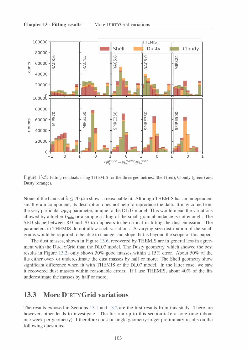
Chapter 13 - Fitting results More DIRTYGrid variations
Figure 13.5: Fitting residuals using THEMIS for the three geometries: Shell (red), Cloudy (green) andDusty (orange).
None of the bands at λ ≤ 70 µm shows a reasonable fit. Although THEMIS has an independentsmall grain component, its description does not help to reproduce the data. It may come fromthe very particular qPAH parameter, unique to the DL07 model. This would mean the variationsallowed by a higher Umin or a simple scaling of the small grain abundance is not enough. TheSED shape between 8.0 and 70 µm appears to be critical in fitting the dust emission. Theparameters in THEMIS do not allow such variations. A varying size distribution of the smallgrains would be required to be able to change said slope, but is beyond the scope of this paper.
The dust masses, shown in Figure 13.6, recovered by THEMIS are in general less in agree-ment with the DIRTYGrid than the DL07 model. The Dusty geometry, which showed the bestresults in Figure 13.2, only shows 30% good masses within a 15% error. About 50% of thefits either over- or underestimate the dust masses by half or more. The Shell geometry showsignificant difference when fit with THEMIS or the DL07 model. In the latter case, we sawit recovered dust masses within reasonable errors. If I use THEMIS, about 40% of the fitsunderestimate the masses by half or more.
13.3 More DIRTYGrid variations
The results exposed in Sections 13.1 and 13.2 are the first results from this study. There arehowever, other leads to investigate. The fits run up to this section take a long time (aboutone week per geometry). I therefore chose a single geometry to get preliminary results on thefollowing questions.
103

Chapter 13 - Fitting results More DIRTYGrid variations
Figure 13.6: Fractional residuals for dust masses using THEMIS. Color code is the same than Figure13.5.
13.3.1 Continuous vs Burst Star formation
I run a fit to compare the differences between a continuous and a burst star formation. In theprevious sections, all fits are done with a continuous star formation. Here, I fit a Dusty geometryonly, as it showed the best results in terms of dust masses in the previous section.
In terms of fits quality, there is no major difference between the two situations. Only theIRAC4.5 and IRAC5.8 bands are better fit in a continuous star formation situation. The otherbands show very similar results.
In terms of dust masses, the instantaneous-type formation follows almost exactly the resultsof the constant formation. A larger portion of the data point are being underestimated in theformer case, by 50−100%.
13.3.2 Clumpy vs Homogeneous dust distribution
I also investigate the differences between a clumpy and a homogeneous distributions of dust inthe Dusty geometry.
Once again, there is no significant difference in terms of fits quality, between the two dis-tributions. Their residuals both follow the same trend: they still exhibit negative wings at longwavelengths, and reasonable fits at shorter wavelengths. This result is quite in opposition withthe study of Witt & Gordon (2000), who showed a clumpy medium was more adequate toreproduce dust extinction, using radiative transfer as well.
The dust mass distributions in both situations are very similar. Contrary to the differenceseen in Section 13.3.1, the residuals overlap almost perfectly, and the homogeneous geometrydoes not show any peculiar result, compared to the Clumpy one.
104

Chapter 13 - Fitting results More DIRTYGrid variations
In both cases, there are few differences between a Burst or Continuous star formation, orbetween a Clumpy or Homogeneous dust distribution. That indicates that dust emission is likelya poor probe to discriminate between these situation in real observations. On the bright side, itmeans that dust emission models do not necessarily need to take these parameters into account,as they do not affect much the resulting properties.
105

Chapter 13 - Fitting results More DIRTYGrid variations
106

14Dust RT: conclusions and perspectives
The goal of this study was to investigate the effects due to to radiative transfer in dust emissionfitting. I used an RT-based library of dust emission SEDs: the DIRTYGrid. The SEDs werecreated by the integration of dust emission spectra in the photometric bands of the SpitzerIRAC and MIPS instruments, and the Herschel SPIRE instrument. The RT calculations aremade in various geometries of stars and dust, representative of the multiple possibilities thatcan be found in nearby galaxies. These SEDs were fit with the common dust models used in theliterature: the Draine & Li (2007) model and THEMIS (Jones et al. 2013). These models use adescription of the dust heating environment simpler than that from the RT calculations.
Using the same dust composition on both sides (RT-based and common model), I have stillidentified some discrepancies between the two approaches. Namely, the shape of the dust SEDin the FIR fails at being adjusted by the classical use of dust models like Draine & Li (2007).The fluxes in the DIRTYGrid are underestimated by the DL07 model. The dust masses recoveredare geometry-dependent. The quality of the results varies from a geometry to the other. This isindicative that the relative distribution of stars and dust is important in dust emission fitting. It isan aspect that simple descriptions of the ISRF fail at reproducing. In all cases, the dust massesare over- or underestimated by less than a factor 2, which is still a good sign, despite the visiblevariations. Unique to the DL07 model, the qPAH parameter is never properly recovered by thefits. It is constantly overestimated. The reason of the peculiar behavior still remains unknown,but a lack, or at least, a shortcoming of a parameter definition in the NIR is likely, additionallyto the RT effects.
I have shown that using a different dust composition may lead to better results in some partof the SED. For instance, THEMIS reproduces better the FIR SED points. However, it fails atadjusting the fluxes in the NIR and MIR. The same conclusion stands for the dust masses usingthis model. Contrary to the DL07 model, no geometry seems to present a good recovery of thedust masses that were put in the DIRTYGrid.
The differences that stand out for each model are interesting as they show their respectiveassets and shortcomings. In all cases, an accurate adjustment of all parameters at once seemsimpossible. However, investigation leads will stem from these results. For instance, a free sizedistribution may strongly improve the quality of the fits. The relative mass distribution in a dustmodel (more weight in the small carbonaceous or the large ones) is also an interesting path to
107

Chapter 14 - Dust RT: conclusions and perspectives
study. More work following this one will continue to make use of the RT-based and the commondust model, to identify and correct the systematic errors due to our simplifications.
To go further, a general question we can study is the impact of the number of bands on thefits. Is this number critical to the results? Is there a minimal number of bands to recover acorrect dust mass, and are there wavelengths to prefer to others? Small and large grains do notemit at the same wavelengths; silicate and large carbonaceous grains emission spectra do nothave the same shape. It is thus interesting to know how our results in modeling IR emission ofnearby galaxies are sensitive to the choice of wavelengths or ranges.For example, what are the wavelengths crucial to constraint the IR peak? Works have shownthat 100 µm is necessary. However, can we think that using both 70 and 160 µm could play thesame role? A lot of studies focus on the FIR/sub-mm part of the dust emission spectrum. In thatcase, modified blackbodies are often used. Understanding which band is critical to constrainthe temperature, and which is critical to the emissivity would bring a useful insights to that typeof study.We can also look closer at the sub-mm and millimeter ranges. Those are the wavelengths wherecold dust emits. In a “cold” environment, dust grains form aggregates; these might be non-negligible and contribute to the dust mass budget. As shown in the first study of this thesis(Part II, Chastenet et al. 2017), the sub-mm is also the frame where a distinction can be madebetween silicate and carbonaceous. It has been shown that their FIR emissivity slope is notidentical; at longer wavelength, the distinction could become more evident and, combined withshorter wavelengths, allow for a clear estimation of each population abundance.The 24-70 µm (or 8-70µm) slope is also interesting as it gives clues about small grain sizedistribution. Constraining these wavelengths may help to constrain shorter wavelengths, butalso have a consequence in our understanding of small grain processing. The project SPICA(Space Infrared telescope for Cosmology and Astrophysics) could be an excellent opportunityto gather data in this wavelength range. Its MIR instrument should provide with data between12 and 36 µm in spectroscopy and around 34 µm in photometry. It would be an excellentcandidate to help constraining the size distribution of small to large grains.
An interesting output of the DIRTYGrid is the distribution of the ISRF computed by the RTroutine in each cell. This is a tremendous information to analyze. The current method to mixtemperatures is based on empirical fittings and results. Looking directly at what distribution ofISRF the RT calculations determine would be a strong indicator of our accuracy. In the future,using this output can reveal more insights about the differences that may exist, for instance,between different geometries. We might expect a different ISRF distribution between the Dustygeometry, where dust and stars are completely mixed, and Cloudy, where the starlight is muchless blocked by dust grains. In these various situations, the relative contributions of ISRFs ofdifferent intensities or hardness may change, and not be similar to a power-law distribution.Determining another empirical law of mixing, or validate the current one, based on RT calcula-tions would be a tremendous step forward. A direct application to nearby galaxies would be agood confirmation (or rejection) of the model findings from RT.
108

Chapter 14 - Dust RT: conclusions and perspectives
PART III − TAKE AWAY
The results presented in this part are gathered in a publication that will be soon submitted.After identifying the differences between models in Part I, we wanted to investigate thebiases due to the assumptions made when using a dust model, in nearby galaxies, and inparticular in the recipes for mixing environment at different U. To do so, we used dustemission SEDs from radiative transfer (RT) calculations, fit with dust models used in theliterature.
What did we show:
• the RT effects do have an impact on the shape of the SEDeven when the dust composition is the same. The dust modeling we use innearby galaxies suffers from a “too simple” description of the ISRF, and from nottaking into account the distribution of dust and stars.
• My results show biases in the dust masses recovered compared to the ones in-put in the synthetic data. These biases are geometry dependent and the over-/underestimations can go up to ∼ 100%.
• Clues of a insufficient parameterization of the MIR are visible. A parameter, theqPAH fraction, shows no good fits, in any of the geometries.
• Using a different dust composition than that built in the grid may lead to a betterfit quality, in some bands; it means the flux recovery is not a strong indicator of theaccuracy of dust description.
This whole study is in a paper in preparation, and the first of a series that will use ex-tensively the comparisons between a synthetic grid and the dust models we use to fit IRemission of nearby galaxies.
109

Chapter 14 - Dust RT: conclusions and perspectives
110

Part IV
General Conclusion & Perspectives
111


General conclusion
The goal of this thesis was to question the impact of the assumptions made while fitting fulldust models to the IR emission of nearby galaxies. For instance, the dust composition betweenmodels changes: graphite or amorphous carbon, and silicates, presence of aromatic mantles,inclusions of metals. This is also true for the grain size distributions: one population or two,extent of the small grains. Different descriptions of the ISRF are also used: power-law mixingof radiation fields, single temperature or mixtures of environments. We can also find differentvalues for the emissivity index β . Despite these differences, all models are designed to fit moreor less the same reference: the dust constraints in the solar neighborhood (emission, extinction,and depletions). But our curiosity goes beyond our galaxy, and we are rightful to ask ourselvesif using this description in other galaxies is appropriate. My thesis work has hence focused onthe impact of assumptions and dust model choices on dust emission modeling in nearby galax-ies.
In a first part, I analyzed the IR emission of two nearby galaxies, the Magellanic Clouds(MCs). I have adjusted their emission from 3.6 to 500 µm with different dust models: Com-piègne et al. (2011), THEMIS, and Draine & Li (2007). This was done using a common fittingtechnique, DustBFF, in order to identify variations in the resulting parameters that would be dueto the choice of the models only.I found that THEMIS (Jones et al. 2013; Köhler et al. 2014; Ysard et al. 2015; Jones et al. 2017)reproduces the observations in the MCs better than the Compiègne et al. (2011) model. Thatis due to a more accurate description of the spectral index in the FIR/submillimeter regime.THEMIS was used in either a single or multiple ISRFs, to investigate the impact of the tem-perature mixing. I showed that using multiple ISRFs to create dust emission spectra leads toa better adjustment of the data. I derived dust properties from the fitting with THEMIS. Thismodel is described by a population of carbonaceous and silicate grains. I showed that theirrelative abundance is different on average between each galaxy and the Milky-Way. Variationswithin each galaxy are also seen. That indicates that the dust composition is different in ourGalaxy from the LMC and the SMC. Dust masses were inferred in this study as well, and are inagreement with previous studies.I used dust properties inferred from emission fitting to create dust extinctions curves, in a fewlines-of-sight in the MCs. I showed that using dust properties derived from emission only re-sults in extinction curves that do not match the observed data. It suggests that dust emissionproperties are not sufficient to completely describes its composition, and that extinction alsoconveys crucial information. These results have been published in Chastenet et al. (2017).
Following this study, I added the Draine & Li (2007) model to the comparison. My resultsindicate that this model provides similar results as THEMIS. Finally, using the same data, andTHEMIS, I also investigated the impact of the ISRF shape, as opposed to its intensity, on thefit quality. I showed that the preferred hardness of the radiation field is different between eachgalaxy.
113

This study highlighted the importance of the dust heating environment on derived properties.The second study presented in this thesis stemmed from this result.
In the second part of my thesis, I explored the implications of the empirical ISRF-mixinglaws on dust emission fitting in nearby galaxies. To do so, I used synthetic data created from ra-diative transfer (RT) calculations (DIRTYGrid: Gordon et al. 2001; Misselt et al. 2001, and Lawet al. in prep.), and fit them as if they were observations of nearby galaxies. The DIRTYGridaims at determining the ISRF in each position within a 3D geometry of stars and dust. Thedust emission spectrum is hence calculated with a more physically-determined ISRF, at eachposition of the cloud. I compared this realistic approach to the dust models used in nearbygalaxies (multi-ISRF model). First, I used the Draine & Li (2007) model as it is the same dustcomposition as in the DIRTYGrid. The differences observed between the best fit parameters andthe grid inputs are therefore only due to RT effects.I showed that the relative distribution of stars and dust has an impact on the inferred dust prop-erties, in particular on dust masses. Although this geometry effect does not affect much thequality of the fits, other parameters can be over- or underestimated depending on the situation.However, my results showed that these discrepancies do not go beyond a factor of 2. Theseresults, presented in a paper to be submitted soon, demonstrate that the empirical mixing lawsused in dust emission modeling of nearby galaxies still suffer shortcomings. Those results arethe first of a series that will make more use of the RT-based calculations and dust model com-parison. The advantage of this approach is that we know the reality of the data, that can bedirectly compared to the results of the fitting.
Those two studies show that the choices and assumptions made in dust modeling for dustemission fitting do have an impact on the inferred dust properties. The difference in dust com-position from a model to another, or the chosen law to mix dust at different temperatures affectestimations of dust masses, grain sizes and relative abundances.The framework developed in this thesis will be further used in the future. In particular, I willexplore the impact of the number of photometric bands, the empirical law of ISRF-mixing, andthe impact of clumpiness and star formation scenario on inferred dust properties.This thesis has presented a direct application only in two nearby galaxies. More extensive workwill be done in a large sample of galaxies at very low redshifts. I will collaborate with Drs.Karin Sandstrom and Adam Leroy on building a catalog of dust, gas and stars in galaxies atredshift z = 0. The vast number of observations will allow me to probe the extent of my resultsin various environments.
114


Bibliography
Allamandola, L. J., Tielens, A. G. G. M., & Barker, J. R. 1985, ApJ, 290, L25
Aniano, G., Draine, B. T., Gordon, K. D., & Sandstrom, K. 2011, PASP, 123, 1218
Asplund, M., Grevesse, N., Sauval, A. J., & Scott, P. 2009, ARA&A, 47, 481
Baes, M., Gordon, K. D., Lunttila, T., et al. 2016, A&A, 590, A55
Balog, Z., Müller, T., Nielbock, M., et al. 2013, Experimental Astronomy
Barnard, E. E. 1910, ApJ, 31
Beitia-Antero, L. & Gómez de Castro, A. I. 2017, MNRAS, 469, 2531
Bendo, G. J., Griffin, M. J., Bock, J. J., et al. 2013, MNRAS, 433, 3062
Bennett, C. L., Banday, A. J., Gorski, K. M., et al. 1996, ApJ, 464, L1
Bernard, J.-P., Reach, W. T., Paradis, D., et al. 2008, AJ, 136, 919
Bocchio, M., Jones, A. P., & Slavin, J. D. 2014, A&A, 570, A32
Bolatto, A. D., Simon, J. D., Stanimirovic, S., et al. 2007, ApJ, 655, 212
Bot, C., Boulanger, F., Lagache, G., Cambrésy, L., & Egret, D. 2004, A&A, 423, 567
Bot, C., Ysard, N., Paradis, D., et al. 2010, A&A, 523, A20
Boulanger, F., Abergel, A., Bernard, J.-P., et al. 1996, A&A, 312, 256
Bradley, J., Dai, Z. R., Erni, R., et al. 2005, Science, 307, 244
Brüns, C., Kerp, J., Staveley-Smith, L., et al. 2005, A&A, 432, 45
Campbell, E. K., Holz, M., Gerlich, D., & Maier, J. P. 2015, Nature, 523, 322
Cardelli, J. A., Clayton, G. C., & Mathis, J. S. 1988, ApJ, 329, L33
Cardelli, J. A., Clayton, G. C., & Mathis, J. S. 1989, ApJ, 345, 245
Cartledge, S. I. B., Clayton, G. C., Gordon, K. D., et al. 2005, ApJ, 630, 355
Chastenet, J., Bot, C., Gordon, K. D., et al. 2017, A&A, 601, A55
Compiègne, M., Verstraete, L., Jones, A., et al. 2011, A&A, 525, A103
Dale, D. A., Helou, G., Contursi, A., Silbermann, N. A., & Kolhatkar, S. 2001, ApJ, 549, 215
117

Dell’Agli, F., García-Hernández, D. A., Ventura, P., et al. 2015, MNRAS, 454, 4235
Demyk, K., Meny, C., Lu, X.-H., et al. 2017, A&A, 600, A123
Desert, F.-X., Boulanger, F., & Puget, J. L. 1990, A&A, 237, 215
D’Onghia, E. & Fox, A. J. 2016, ARA&A, 54, 363
Donn, B. 1968, ApJ, 152, L129
Draine, B. T. 2003a, ARA&A, 41, 241
Draine, B. T. 2003b, ApJ, 598, 1026
Draine, B. T., Dale, D. A., Bendo, G., et al. 2007, ApJ, 663, 866
Draine, B. T. & Lee, H. M. 1984, ApJ, 285, 89
Draine, B. T. & Li, A. 2001, ApJ, 551, 807
Draine, B. T. & Li, A. 2007, ApJ, 657, 810
Engelbracht, C. W., Blaylock, M., Su, K. Y. L., et al. 2007, PASP, 119, 994
Engelbracht, C. W., Rieke, G. H., Gordon, K. D., et al. 2008a, ApJ, 685, 678
Engelbracht, C. W., Rieke, G. H., Gordon, K. D., et al. 2008b, ApJ, 678, 804
Fazio, G. G., Hora, J. L., Allen, L. E., et al. 2004, ApJS, 154, 10
Fioc, M. & Rocca-Volmerange, B. 1997, A&A, 326, 950
Fioc, M. & Rocca-Volmerange, B. 1999, ArXiv Astrophysics e-prints
Fitzpatrick, E. L. 1999, PASP, 111, 63
Fitzpatrick, E. L. & Massa, D. 2005, AJ, 130, 1127
Galametz, M., Madden, S. C., Galliano, F., et al. 2011, A&A, 532, A56
Galliano, F., Hony, S., Bernard, J.-P., et al. 2011, A&A, 536, A88
Galliano, F., Madden, S. C., Jones, A. P., Wilson, C. D., & Bernard, J.-P. 2005, A&A, 434, 867
Galliano, F., Madden, S. C., Jones, A. P., et al. 2003, A&A, 407, 159
Gaustad, J. E., McCullough, P. R., Rosing, W., & Van Buren, D. 2001, PASP, 113, 1326
Gordon, K. D., Cartledge, S., & Clayton, G. C. 2009, ApJ, 705, 1320
Gordon, K. D. & Clayton, G. C. 1998, ApJ, 500, 816
Gordon, K. D., Clayton, G. C., Misselt, K. A., Landolt, A. U., & Wolff, M. J. 2003, ApJ, 594,279
Gordon, K. D., Engelbracht, C. W., Fadda, D., et al. 2007, PASP, 119, 1019
118

Gordon, K. D., Galliano, F., Hony, S., et al. 2010, A&A, 518, L89
Gordon, K. D., Meixner, M., Meade, M. R., et al. 2011, AJ, 142, 102
Gordon, K. D., Misselt, K. A., Witt, A. N., & Clayton, G. C. 2001, ApJ, 551, 269
Gordon, K. D., Roman-Duval, J., Bot, C., et al. 2014, ApJ, 797, 85
Graczyk, D., Pietrzynski, G., Thompson, I. B., et al. 2014, ApJ, 780, 59
Griffin, M. J., Abergel, A., Abreu, A., et al. 2010, A&A, 518, L3
Griffin, M. J., North, C. E., Schulz, B., et al. 2013, MNRAS, 434, 992
Harris, J. 2007, ApJ, 658, 345
Heck, P. R., Gyngard, F., Ott, U., et al. 2009, ApJ, 698, 1155
Heger, M. L. 1922, Lick Observatory Bulletin, 10, 146
Henning, T. & Mutschke, H. 1997, A&A, 327, 743
Hobbs, L. M., York, D. G., Thorburn, J. A., et al. 2009, ApJ, 705, 32
Houck, J. R., Roellig, T. L., van Cleve, J., et al. 2004, ApJS, 154, 18
Hughes, A., Wong, T., Ott, J., et al. 2010, MNRAS, 406, 2065
Israel, F. P., Wall, W. F., Raban, D., et al. 2010, A&A, 519, A67
Jarosik, N., Bennett, C. L., Dunkley, J., et al. 2011, ApJS, 192, 14
Jenkins, E. B. 2009, ApJ, 700, 1299
Jenniskens, P. & Desert, F.-X. 1994, A&AS, 106
Jones, A. P. 2012a, A&A, 545, C2
Jones, A. P. 2012b, A&A, 545, C3
Jones, A. P. 2012c, A&A, 540, A1
Jones, A. P. 2012d, A&A, 540, A2
Jones, A. P. 2012e, A&A, 542, A98
Jones, A. P., Fanciullo, L., Köhler, M., et al. 2013, A&A, 558, A62
Jones, A. P., Köhler, M., Ysard, N., Bocchio, M., & Verstraete, L. 2017, A&A, 602, A46
Keller, S. C. & Wood, P. R. 2006, ApJ, 642, 834
Kennicutt, Jr., R. C., Armus, L., Bendo, G., et al. 2003, PASP, 115, 928
Kim, S., Staveley-Smith, L., Dopita, M. A., et al. 2003, ApJS, 148, 473
Köhler, M., Jones, A., & Ysard, N. 2014, A&A, 565, L9
119

Köhler, M., Ysard, N., & Jones, A. P. 2015, A&A, 579, A15
Kroto, H. W. & Jura, M. 1992, A&A, 263, 275
Le Bourlot, J., Le Petit, F., Pinto, C., Roueff, E., & Roy, F. 2012, A&A, 541, A76
Leger, A. & Puget, J. L. 1984, A&A, 137, L5
Leroy, A., Bolatto, A., Stanimirovic, S., et al. 2007, ApJ, 658, 1027
Lewis, N. K., Cook, T. A., Wilton, K. P., et al. 2009, ApJ, 706, 306
Li, A. & Draine, B. T. 2001, ApJ, 554, 778
Marigo, P., Girardi, L., Bressan, A., et al. 2008, A&A, 482, 883
Mathis, J. S. 1990, ARA&A, 28, 37
Mathis, J. S., Mezger, P. G., & Panagia, N. 1983, A&A, 128, 212
Mathis, J. S., Rumpl, W., & Nordsieck, K. H. 1977, ApJ, 217, 425
Mathis, J. S., Whitney, B. A., & Wood, K. 2002, ApJ, 574, 812
Mattila, K. 1970, A&A, 9, 53
Mattila, K., Lemke, D., Haikala, L. K., et al. 1996, A&A, 315, L353
Meisner, A. M. & Finkbeiner, D. P. 2015, ApJ, 798, 88
Meixner, M., Gordon, K. D., Indebetouw, R., et al. 2006, AJ, 132, 2268
Meixner, M., Panuzzo, P., Roman-Duval, J., et al. 2013, AJ, 146, 62
Meixner, M., Panuzzo, P., Roman-Duval, J., et al. 2015, AJ, 149, 88
Merrill, P. W. 1934, PASP, 46, 206
Merrill, P. W. & Wilson, O. C. 1934, ApJ, 80, 19
Mezger, P. G., Mathis, J. S., & Panagia, N. 1982, A&A, 105, 372
Misselt, K. A., Gordon, K. D., Clayton, G. C., & Wolff, M. J. 2001, ApJ, 551, 277
Mizuno, N., Rubio, M., Mizuno, A., et al. 2001, PASJ, 53, L45
Molinari, S., Swinyard, B., Bally, J., et al. 2010, PASP, 122, 314
Müller, T., Nielbock, M., Balog, Z., Klaas, U., & Vilenius, E. 2011, PACS Photometer - Point-Source Flux Calibration, Tech. Rep. PICC-ME-TN-037, Herschel
Nanni, A., Bressan, A., Marigo, P., & Girardi, L. 2013, MNRAS, 434, 2390
Neugebauer, G., Habing, H. J., van Duinen, R., et al. 1984, ApJ, 278, L1
Ochsenbein, F., Bauer, P., & Marcout, J. 2000, A&AS, 143, 23
120

Oort, J. H. & van de Hulst, H. C. 1946, Bull. Astron. Inst. Netherlands, 10, 187
Paradis, D., Paladini, R., Noriega-Crespo, A., et al. 2012, A&A, 537, A113
Paradis, D., Reach, W. T., Bernard, J.-P., et al. 2009, AJ, 138, 196
Pilbratt, G. L., Riedinger, J. R., Passvogel, T., et al. 2010, A&A, 518, L1
Planck Collaboration, Abergel, A., Ade, P. A. R., et al. 2014, A&A, 566, A55
Platt, J. R. 1956, ApJ, 123, 486
Poglitsch, A., Waelkens, C., Geis, N., et al. 2010, A&A, 518, L2
Purcell, E. M. & Pennypacker, C. R. 1973, ApJ, 186, 705
Putman, M. E., Staveley-Smith, L., Freeman, K. C., Gibson, B. K., & Barnes, D. G. 2003, ApJ,586, 170
Reach, W. T., Dwek, E., Fixsen, D. J., et al. 1995, ApJ, 451, 188
Reach, W. T., Megeath, S. T., Cohen, M., et al. 2005, PASP, 117, 978
Rémy-Ruyer, A., Madden, S. C., Galliano, F., et al. 2014, A&A, 563, A31
Rieke, G. H., Young, E. T., Engelbracht, C. W., et al. 2004, ApJS, 154, 25
Rolleston, W. R. J., Trundle, C., & Dufton, P. L. 2002, A&A, 396, 53
Roman-Duval, J., Gordon, K. D., Meixner, M., et al. 2014, ApJ, 797, 86
Roman-Duval, J., Jackson, J. M., Heyer, M., Rathborne, J., & Simon, R. 2010, ApJ, 723, 492
Russell, S. C. & Dopita, M. A. 1992, ApJ, 384, 508
Sandstrom, K. M., Bolatto, A. D., Bot, C., et al. 2012, ApJ, 744, 20
Sandstrom, K. M., Bolatto, A. D., Draine, B. T., Bot, C., & Stanimirovic, S. 2010, ApJ, 715,701
Stanimirovic, S., Staveley-Smith, L., & Jones, P. A. 2004, ApJ, 604, 176
Stanimirovic, S., Staveley-Smith, L., van der Hulst, J. M., et al. 2000, MNRAS, 315, 791
Staveley-Smith, L., Kim, S., Calabretta, M. R., Haynes, R. F., & Kesteven, M. J. 2003, MNRAS,339, 87
Steinacker, J., Baes, M., & Gordon, K. D. 2013, ARA&A, 51, 63
Stock, D. J. & Peeters, E. 2017, ApJ, 837, 129
Tchernyshyov, K., Meixner, M., Seale, J., et al. 2015, ApJ, 811, 78
Trumpler, R. J. 1930, PASP, 42, 214
van der Marel, R. P. & Kallivayalil, N. 2014, ApJ, 781, 121
121

Volten, H., Muñoz, O., Hovenier, J. W., et al. 2007, A&A, 470, 377
Walker, A. R. 2012, Ap&SS, 341, 43
Weingartner, J. C. & Draine, B. T. 2001, ApJ, 548, 296
Welty, D. E., Lauroesch, J. T., Blades, J. C., Hobbs, L. M., & York, D. G. 2001, ApJ, 554, L75
Werner, M. W., Roellig, T. L., Low, F. J., et al. 2004, ApJS, 154, 1
Whitney, B. A. 2011, Bulletin of the Astronomical Society of India, 39, 101
Witt, A. N. & Gordon, K. D. 2000, ApJ, 528, 799
Witt, A. N. & Stephens, T. C. 1974, AJ, 79, 948
Ysard, N., Köhler, M., Jones, A., et al. 2015, A&A, 577, A110
Zubko, V., Dwek, E., & Arendt, R. G. 2004, ApJS, 152, 211
Zubko, V. G., Mennella, V., Colangeli, L., & Bussoletti, E. 1996, MNRAS, 282, 1321
122

Part V
Annexes
123


AExtinctions curves
Here I show the results for my estimation of extinction curves based on dust properties derivedfrom dust emission fitting. There are 4 lines of sight in the SMC, and 19 in the LMC, all labelledwith the star used to measure the extinction curve.
125

Figure A.1: Extinction curves in the SMC observed by Gordon et al. (2003) (grey circles), and themodeled curves created from emission-derived dust parameters (see Section 8.2).
126

Figure A.2: Extinction curves in the LMC observed by Gordon et al. (2003) (grey circles), and themodeled curves created from emission-derived dust parameters (see Section 8.2).
127

Figure A.3: Figure A.2 continued.
128

Figure A.4: Figure A.2 continued.
129

Figure A.5: Figure A.2 continued.
130

Figure A.6: Figure A.2 continued.
131

132

BTHEMIS parameters: triangular plots
I present here the triangular plots for two environments of Part II: a single ISRF and multi-ISRFs. This type of figure aims at showing possible degeneracies between parameters. We donot see strong variations between both approaches, and a slight difference between the galaxies,when it comes to the aSilM5 parameter.
133

Figure B.1: Triangular plots showing parameter relationships for THEMIS in a Single-U environmentin the MC (top) and LMC (bottom).

Figure B.2: Same as Figure B.1 in a Multi-U environment.


UNIVERSITÉ DE STRASBOURG
ÉCOLE DOCTORALE Physique, Chimie-Physique
UMR 7550
THÈSE présentée par :
Jérémy CHASTENET soutenue le : 26 septembre 2017
pour obtenir le grade de : Docteur de l’université de Strasbourg
Discipline/Spécialité : Astrophysique
Analyse de l’émission des poussières dans les galaxies proches
Impact des hypothèses et choix des modèles
THÈSE dirigée par : Mme BOT Caroline Astronome adjointe, Observatoire astronomique de Strasbourg M. GORDON Karl Astronome, Space Telescope Science Institute
RAPPORTEURS : Mme MADDEN Suzanne Ingénieur CEA, CEAM. BAES Maarten Professeur en Astrophysique, Sterrenkundig Observatorium
AUTRES MEMBRES DU JURY : Mme DEMYK Karine Directrice de Recherche, IRAP Mme GENOVA Françoise Directrice de Recherche, Observatoire astronomique de Strasbourg M. CAMBRESY Laurent Astronome, Observatoire astronomique de Strasbourg


Introduction généraleL’espace est rempli d’une quantité considérable d’objets d’une grande variété : des étoiles dedifférentes masses, des galaxies de différentes formes, des planètes lointaines et d’immensesnuages de gaz et de tout petits grains de poussières.Pendant ma thèse, je me suis attaché à étudier ce que l’on appelle la poussière. Il s’agit depetits grains solides associés au gaz, dont la taille varie entre le nanomètre et le micromètre.On trouve ces grains de poussière dans les disques de formation planétaire ou dans un milieudit interstellaire : l’espace entre les étoiles, au sein d’une galaxie. Nous nous intéresserons enparticulier à cette poussière interstellaire, et plus précisément, celle que l’on peut trouver dansles galaxies proches de la notre.Avant toute chose, revoyons brièvement les différentes parties du spectre électromagnétique, lesinformations qu’elles relaient, et le domaine d’étude de cette thèse.Les rayons Gamma permettent d’observer les objets très énergétiques et/ou très chauds, telsque des étoiles à neutrons ou les alentours des trous noirs. Les rayons-X sont caractéristiquesd’objets un peu moins chauds comme du gaz à haute température ou les restes d’une supernova.L’ultraviolet (UV) rend compte principalement de l’émission des étoiles jeunes, tandis que desétoiles plus vieilles sont visibles dans le domaine optique (observable à l’oeil nu). Dans ledomaine infrarouge (IR), on observe majoritairement l’émission de la poussière, et ce sontces longueurs d’onde qui vont nous intéresser, de quelques micromètres à un peu moins d’unmillimètre. Enfin, les ondes radio nous permettent de voir la matière froide, comme du gaz àbasse température ou des nuages moléculaires.
Région HII
Milieu diffus
Nuage moléculaire
Supernova Géante rouge
Etoile massive Etoile faible
masse
Proto-étoile
Dense core
ionisation
formation
d’éléments
formation
d’éléments
Région HII
Milieu diffus
Nuage moléculaire
Supernova Géante rouge
Etoile massive Etoile faible
masse
Proto-étoileProto-étoile
Dense core
ionisation
formation
d’éléments
formation formation
d’éléments
Grains
standards
Aggrégats
Glaces
Manteaux
Petits
grains
Figure B.3: Schéma simplifié du cycle du MIS.
Puisque nous nous intéressons àla poussière interstellaire, il con-vient d’introduire un peu le mi-lieu qu’elle constitue avec le gaz: le milieu interstellaire (MIS).Les grains de poussière évoluentselon un cycle dans le MIS. Par-tons du nuage moléculaire, sur laFigure B.3 : c’est un dense nu-age de gaz, principalement com-posé de H2. On y trouve desagglomérats de grains, collés en-tre eux, avec d’épais manteaux,possiblement faits de glace (H2O,CO2). Ce nuage moléculaire peutdonner vie à des étoiles s’il de-vient assez dense et s’effondre surlui-même. La génération d’étoilesainsi formées créent des élémentslourds par nucléosynthèse. Ces
éléments se retrouvent dans les grains de poussière, qui font leur apparition dans les enveloppesd’étoiles relativement massives. Par la suite, ces nouvelles étoiles génèrent des photons UVcapables d’ioniser les atomes d’hydrogène alentours. S’ils sont suffisamment énergétiques, ilspeuvent également éroder, voire briser, les grains de poussière. Cette région ionisée est dénom-mée région H II. Ces grains sont “rendus” au milieu diffus. La formation d’un nouveau nuagedense dépend de la gravité ; la coagulation des grains est possible dans ces nuages. La com-position et la taille des grains varient d’une région à l’autre. On définit la distribution de taille
3

standard de la poussière par celle du milieu diffus. Pour étudier la poussière dans ces régions,on définit aussi le champ de rayonnement. Il s’agit du spectre d’énergie des photons reçus parles grains. C’est une donnée importante qui impacte directement l’émission IR de la poussière,puisque c’est cette énergie qui sert à chauffer les grains. Mezger et al. (1982) et Mathis et al.(1983) ont produit plusieurs de ces spectres pour décrire le champs de rayonnement à différentesdistances du centre galactique. La référence très souvent utilisée est celle à DG = 10 kpc, dis-tance du Soleil au Centre galactique estimée à l’époque. En utilisant cette information, et leséquations de la physique du solide, nous pouvons maintenant dresser quelques caractéristiquesimportantes de la poussière.
Description de la poussière interstellaireLa poussière peut s’observer par différents moyens : par son extinction, sa capacité à absorberet diffuser les rayons UV, son émission dans l’IR ou sa polarisation avec le champ magnétique.Il est important de décrire correctement la poussière, afin de créer des modèles adéquats quireproduisent les observations, et pouvoir en déduire des propriétés dans les galaxies autres quela notre.
Figure B.4: Haut : Spectre d’émission (Compiègne et al.2011). Bas : Courbe d’extinction (Fitzpatrick 1999).
Extinction L’intensité de la lumièrepassant dans un nuage de poussièreest atténuée, en fonction du nom-bre et de la composition des partic-ules présentes et de la densité du nu-age. Le terme d’extinction Aλ varieselon la section efficace d’extinctionCext(a,λ ) = Qext(a,λ ) πa2. L’efficacitéd’extinction Qext(a,λ ) traduit les pro-priétés des grains de poussière consid-érés.L’extinction est l’effet cumulé de deuxprocessus : l’absorption et la diffusion.Le premier décrit la capacité des grainsà absorber un photon UV, qui provoqueune augmentation de l’énergie interne dugrain. Le second processus décrit la redi-rection des photons UV lorsqu’ils heur-tent un grain de poussière : l’énergiedu photon est la même, mais sa direc-tion change. Lorsque la longueur d’ondede l’onde incidente est plus grande quela taille du grain, plus le grain est petit,plus l’absorption l’emporte sur la diffu-sion.Les variations de l’extinction avec la longueur d’onde sont en général montrées par une courbed’extinction normalisée dans la bande V, comme sur la Figure B.4. Elle montre les particularitésde l’extinction comme la bosse à 2175 Å, ou la pente à grand 1/λ .La distribution de taille des grains est estimée principalement par ces observations. Les modèlesprédisent que les grains couvrent un intervalle de taille assez large, allant de 0.01 à 0.2 µm.
4

Émission L’émission de la poussière dépend de la quantité d’énergie qu’elle absorbe. On dis-tingue en général deux types d’émission des grains. Les grains suffisamment gros sont soumisà un flux incident constant de photons, et ré-émettent cette énergie en continu. On décrit cetteémission par un corps noir modifié, en utilisant la fonction de Planck B(λ ,Td). La pente dansl’infrarouge lointain est modifiée par l’émissivité des grains, qui traduit leur capacité à absorberet émettre la lumière. Si le grain est trop petit pour absorber des photons continuellement, onparle de chauffage stochastique. A chaque absorption d’un photon, un grain de poussière voitson énergie interne et sa température augmenter de façon drastique, avant de se refroidir lente-ment, jusqu’au prochain impact. Ce type de chauffage est décrit dans les modèles de façondifférente. La Figure B.4 montre un exemple de spectre d’émission avec ses différents parties.Dans l’infrarouge moyen (3 µm ≤ λ ≤ 30 µm), les pics d’émission sont caractéristiques desmodes de vibrations de grosses molécules identifiées comme étant des hydrocarbonés aroma-tiques polycycliques (PAH).
Composition chimique La teneur en éléments des grains de poussière est cruciale pour êtreà même de reproduire les observations. En combinant les équations qui décrivent l’extinctionet les observations, il est possible de déduire le volume occupé par les grains de poussière,relativement à celui des atomes d’hydrogène. Cela permet de mettre une limite sur la massede la poussière, et d’en déduire que d’autres éléments que l’hydrogène ou l’hélium contribuentforcément à cette masse.En mesurant les raies d’absorption du gaz interstellaire, on peut en déterminer la compositionchimique : carbone, oxygène, magnésium, silicium, fer... Il est également possible de connaitrela composition chimique du voisinage solaire (cette valeur est souvent utilisée comme référencepour l’abondance totale en éléments du MIS). La composition de la poussière est déduite par cequ’on appelle la déplétion : la différence entre l’abondance observée d’une étoile représentativedu MIS étudié et celle du gaz.
Modèles de grains En utilisant les informations précédemment développées, il est possiblede construire un modèle (dans cette thèse, il s’agit de modèles d’émission) décrivant les pro-priétés physico-chimiques des grains, afin de reproduire les observations de galaxies.Les modèles les plus simples s’intéressent uniquement à l’émission des gros grains. Ils utilisentun corps noir modifié par différentes approches : une simple loi de puissance pour décrirel’émissivité des grains à grand λ , deux lois de puissance, ou encore deux populations de grainsà deux températures différentes (voir Gordon et al. 2014).Des modèles plus complets couvrent une plus large distribution de taille de grains, et prédis-ent un spectre d’émission du proche infrarouge au sub-millimétrique. On peut nommer parexemple :
• Draine & Li (2007, DL07) : qui émerge des travaux de Draine & Lee (1984), avec desmises à jour sur la taille et physique des grains (Draine & Li 2001; Li & Draine 2001;Weingartner & Draine 2001). Ce modèle utilise une population de carbone graphite et unepopulation de grains silicatés. C’est le modèle le plus utilisé pour modéliser la poussière.
• Compiègne et al. (2011) : s’inspire du modèle de Desert et al. (1990), avec des modifica-tions venant des travaux de Draine & Lee (1984), Zubko et al. (1996), Draine (2003b) etDraine & Li (2007).
• THEMIS1 : développé par Jones et al. (2013), Köhler et al. (2014) et Ysard et al. (2015),ce modèle accorde une place importante à de nouvelles mesures en laboratoire (Jones2012c,d,a,e,b). Ce modèle décrit la poussière par des grains carbonés aliphatiques et desgrains silicatés, chacun recouvert d’un manteau aromatique.
1The Heterogeneous Evolution dust Model at the IAS.
5
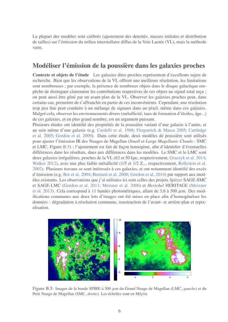
La plupart des modèles sont calibrés (ajustement des densités, masses initiales et distributionde tailles) sur l’émission du milieu interstellaire diffus de la Voie Lactée (VL), mais la méthodevarie.
Modéliser l’émission de la poussière dans les galaxies prochesContexte et objets de l’étude Les galaxies dites proches représentent d’excellents sujets derecherche. Bien que les observations de la VL offrent une meilleure résolution, les limitationssont nombreuses ; par exemple, la présence de nombreux objets dans le disque galactique em-pêche de distinguer clairement les contributions respectives de ces objets au signal total reçu ;on peut aussi être gêné par un avant-plan de la VL. Observer les galaxies proches peut, danscertains cas, permettre de s’affranchir en partie de ces inconvénients. Cependant, une résolutiontrop peu fine peut conduire à un mélange de signaux dans un pixel, même dans ces galaxies.Malgré cela, observer les environnements divers (métallicité, taux de formation d’étoiles, âge...)de ces galaxies, et en plus grand nombre, est un argument puissant.Plusieurs études ont identifié des propriétés de la poussière variant d’une galaxie à l’autre, etau sein même d’une galaxie (e.g. Cardelli et al. 1988; Fitzpatrick & Massa 2005; Cartledgeet al. 2005; Gordon et al. 2009). Dans cette étude, deux modèles de poussière sont utiliséspour ajuster l’émission IR des Nuages de Magellan (Small et Large Magellanic Clouds : SMCet LMC, Figure B.5) ; l’ajustement est fait de façon homogène, afin d’identifier d’éventuellesdifférences dans les résultats, dues aux différences dans les modèles. Le SMC et le LMC sontdeux galaxies irrégulières, proches de la VL (62 et 50 kpc, respectivement, Graczyk et al. 2014;Walker 2012), avec une plus faible métallicité (1/5 et 1/2 Z⊙, respectivement, Rolleston et al.2002). Plusieurs travaux se sont intéressés à ces galaxies, et ont notamment identifié des excèsd’émission (e.g. Bot et al. 2004; Bernard et al. 2008; Gordon et al. 2014) par rapport aux mod-èles existants. Les observations que j’ai utilisées ici sont celles des projets Spitzer SAGE-SMCet SAGE-LMC (Gordon et al. 2011; Meixner et al. 2006) et Herschel HERITAGE (Meixneret al. 2013). Cela correspond à 11 bandes photométriques, allant de 3,6 à 500 µm. Des mod-ifications communes aux deux lots d’images ont été mises en place afin d’homogénéiser lesdonnées : dégradation à résolution commune, soustraction de l’avant- et arrière-plan et repix-elisation.
Figure B.5: Images de la bande SPIRE à 500 µm du Grand Nuage de Magellan (LMC, gauche) et duPetit Nuage de Magellan (SMC, droite). Les échelles sont en MJy/sr.
6

Outils utilisés Afin de créer les spectres d’émission à ajuster aux données, j’ai utilisé l’outilDustEM (Compiègne et al. 2011). Pour une composition donnée, avec les valeurs liées auxpropriétés des grains choisis (Q, C, distribution de taille...), DustEM calcule l’extinction etl’émission de la poussière considérée, soumise à un champ de rayonnement (par défaut, celuide Mathis et al. 1983, à 10 kpc). Le modèle de Compiègne et al. (2011, MC11) et THEMIS sontutilisés dans cette étude. Ils divergent par la nature des grains pris en compte (MC11 utilise unepopulation de PAH, tandis que THEMIS modélise ceci par des manteaux aromatiques), la pentedans l’IR lointain (grains silicatés et carbonés ont le même indice spectral dans MC11, différentdans THEMIS), et leurs propriétés optiques et thermiques. Dans chaque cas, les paramètreslibres sont : les abondances de chaque population de grains (3 par modèle), l’intensité du champde rayonnement incident, et une composante stellaire (modélisée par un corps noir), soit aumoins 5 degrés de liberté. Chaque spectre est intégré dans les mêmes bandes photométriquesque les observations, résultant en des distributions spectrales d’énergie (SEDs).L’ajustement des modèles aux données est faite avec DustBFF (Gordon et al. 2014). Il s’agitd’une méthode de calcul qui propage les incertitudes à l’aide de matrices de covariance ; ellesdécrivent les erreurs instrumentales sur les mesures et l’arrière-plan dans les données. Celapermet de tenir compte des corrélations entre les bandes d’observations. La probabilité qu’unmodèle ajuste les données est calculé par un χ2 qui prend en compte la matrice en question.Par ailleurs, cette méthode est aussi intéressante car elle définit des priors pour les valeurs desparamètres considérés. Cela prend en compte des probabilités constantes dans les intervalleschoisis.
Comparaison des modèles Pour cette étude, j’ai créé les spectres d’émission de la poussièredans différents environnements. J’ai étudié plusieurs cas :
• un champ de rayonnement unique ;• deux champs à différentes intensités, créant deux spectres d’émission – un ‘chaud’ et un
‘froid’ – qui résultent en un spectre unique à l’aide d’un paramètre réglant la fractionchaude/froide (Meisner & Finkbeiner 2015) ;
• une combinaison de spectres d’émission à différentes intensités de champs de rayon-nement, résultant en un spectre unique par une intégration en loi de puissance (Dale et al.2001).
Dans le premier cas, un champ de rayonnement unique, THEMIS reproduit mieux les observa-tions que le modèle MC11. En particulier, dans le SMC, les résidus (νIdata
ν − νImodelν )/νIdata
ν
à λ ≥ 100 µm montrent un mauvais ajustement de la pente dans l’IR lointain par le mod-èle MC11. Cela est dû à un indice spectral unique, qui représente mal l’aspect plus plat dela SED à grandes longueurs d’onde. Au contraire, l’indice spectral des grains carbonés deTHEMIS s’accorde mieux à cette forme, et permet un meilleur ajustement des données. Acourtes longueurs d’onde, λ ≤ 8 µm, les deux modèles montrent de larges résidus (c’est-à-dire beaucoup d’erreurs), mais ceux du modèle MC11 sont plus centrés en 0, ce qui équivaut àun meilleur ajustement global. Ceci est vraisemblablement dû à la population des PAH de cemodèle, qui permet un meilleur ajustement dans ces bandes que la population des petits grainscarbonés de THEMIS. Néanmoins, l’ajustement des bandes à 70 et 100 µm par le modèle MC11est moins bon que celui obtenu par THEMIS. Globalement, THEMIS montre donc de meilleursrésultats.Dans les deuxième et troisième cas (plusieurs champs de rayonnements), seul THEMIS estétudié en détail. Les résultats montrent qu’utiliser plusieurs champs de rayonnement, qui per-met de prendre en compte les mélanges le long de la ligne de visée, permet de mieux ajuster lesdonnées. En particulier, la pente entre 8 et 70 µm est mieux reproduite par un environnementavec des champs de rayonnements intégrés en loi de puissance. Cela conduit à une meilleure
7

reproduction des données dans les courtes longueurs d’ondes (λ ≤ 24 µm). D’un point de vuegénéral, utiliser plusieurs champ de rayonnement permet de mieux centrer les résidus, ce quidémontre un meilleur ajustement des données, tant dans le SMC que dans le LMC.Une autre approche est testée, pour tenter de reproduire mieux les bandes à λ ≤ 70 µm :la distribution de tailles des petits grains carbonés est laissée libre, en utilisant un champ derayonnement unique. Cette méthode montre également de meilleurs résultats que la premièreapproche : à courtes longueurs d’onde, les résidus sont plus centrés en 0.
Propriétés des poussières dans les Nuages de Magellan Les propriétés des poussières dansle SMC et le LMC ont été déduites uniquement avec les résultats THEMIS.Les variations spatiales des abondances de chaque population de grains (petits et gros grainscarbonés et grains silicatés) montrent d’importantes variations entre elles, et selon le typed’environnement choisi. La quantité de gros grains carbonés est celle qui varie la moins d’unesituation à l’autre, et est estimée avec de faibles incertitudes.En revanche, seule une limite supérieure peut être posée quant à la quantité de grains silicatés.Les fonctions de probabilités de ce paramètre, dans la plupart des pixels, sont très plates ; cela setraduit par un ajustement équivalent quelque soit la quantité proposée, si elle est en-dessous dela limite. Le nombre de pixels montrant ce genre de résultats est de plus de 50% dans le SMC etd’environ 10% dans le LMC. En moyenne, la limite supérieure est de YaSilM5 ∼ 2,5 MaSilM5
⊙ /MH,identique dans les deux galaxies. Ce résultat impacte directement le rapport SiO2/C. Estimé à∼ 10 dans la VL, il varie entre 0,2 et 0,7 dans le SMC, et entre 0,3 et 1 dans le LMC. Ceciimplique que la composition de la poussière n’est pas la même entre la VL et les Nuages deMagellan.
Figure B.6: Résumé des masses de poussière déduitesdans mon étude, et quelques travaux précédents.
Un point important, et utile à la compara-ison des résultats d’une étude à l’autre,est la masse totale de poussière es-timée dans chaque galaxie. Dans leSMC, j’obtiens (2,9 − 8,9)× 104 M⊙
et (3,7 − 4,2)× 105 M⊙ dans le LMC(Figure B.6). Ces valeurs sont légère-ment plus faibles que celles de l’étudefaite par Gordon et al. (2014), en util-isant uniquement les bandes Herschel.Les erreurs considérées viennent directe-ment de la qualité des ajustements, don-née par le calcul, pour chaque pixel. J’aiégalement calculé les rapports gaz-sur-poussière (GDR) : il s’agit du rapport enmasse de la quantité totale de gaz (dansce cas : hydrogène uniquement) et decelle de poussière. La masse de gaz estcalculée par des observations en H I et CO (e.g. Stanimirovic et al. 2000; Mizuno et al. 2001).En considérant les résultats montrant les meilleurs résidus, les GDRs s’échelonnent entre 1000et 1200 dans le SMC et entre 500 et 520 dans le LMC. Dans le SMC, les variations du GDRen fonction du choix du champ de rayonnement sont assez larges. Des études n’utilisant pasl’émission IR de la poussière ont aussi estimé des GDRs dans les Nuages de Magellan (e.g.Gordon et al. 2003; Tchernyshyov et al. 2015). Bien que les écarts puissent être parfois larges,mes résultats s’accordent raisonnablement avec ces résultats.
8

Impact pour d’autres études En utilisant ces résultats, je me suis intéressé à d’autres prob-lèmes.Par exemple, j’ai créé des courbes d’extinctions en utilisant les abondances dérivées des ajuste-ment à l’émission. J’ai comparé ces courbes d’extinction à des mesures faites dans le SMC etLMC par Gordon et al. (2003). J’ai pu montrer qu’utiliser uniquement les propriétés liées àl’émission IR ne permet pas de reproduire l’extinction, et que les deux observables sont com-plémentaires.J’ai aussi créé des spectres d’émission comme précédemment, mais en utilisant les champs derayonnement construits par Mathis et al. (1983) à d’autres distances DG. J’ai pu montrer queles résultats dans le SMC et le LMC quant à la force (ou distance) du champ de rayonnementqui ajuste le mieux les données sont différents.
Conclusions Cette étude a permis de démontrer que tous les modèles ne reproduisent pasaussi bien les données de galaxies proches comme les nuages de Magellan, bien qu’ils soienttous ajustés sur la VL. Cela a mis en évidence une composition de la poussière différente entrela VL, le SMC et le LMC. Les résultats ont aussi montré que les hypothèses de modélisation(i.e. d’environnement) peuvent affecter lourdement les propriétés déduites de la poussière.
Erreurs systématiques dans la modélisation de la poussièreL’étude précédente a démontré l’importance des choix faits dans la modélisation de l’émissionIR de la poussière. Dans la seconde partie de ma thèse, je me suis intéressé à quantifier plusclairement les erreurs systématiques liées à ces choix. J’ai utilisé une méthode de transfertradiatif pour créer des spectres d’émission dont les propriétés sont connues ; j’ai ajusté cesspectres en les considérant comme des données observationnelles, avec les modèles couram-ment employés dans la littérature. Ces deux approches diffèrent dans la description du champde rayonnement qui chauffe les grains. Dans le cas du transfert radiatif, ce champ est calculé enprenant en compte les interactions possibles ; dans le cas des modèles utilisés pour ajuster lesdonnées, il est décrit empiriquement. Comparer ces deux approches est donc intéressant pouren comprendre les différences.
Transfert radiatif Les méthodes de transfert radiatif (TR) consistent à modéliser le déplace-ment d’une onde/d’un paquet de photons dans un milieu ; dans le cas présent, ce milieu estun mélange d’étoiles et de poussière. Comme décrit précédemment, les grains de poussièreabsorbent la lumière UV et visible, et émettent un rayonnement IR. Ces interactions et contri-butions au spectre électromagnétique sont complexes, et les méthodes les plus simples de mod-élisation de l’émission IR n’en tiennent pas toujours compte. Le TR tend à palier ce problème,et cherche à résoudre l’intensité du champ de rayonnement en chaque position xxx, direction nnn etlongueur d’onde λ d’une certaine géométrie en 3 dimensions. Il s’agit néanmoins d’une méth-ode lourde à mettre en oeuvre : le problème est non-linéaire et non-local, et il n’existe pas desolution analytique. La prise en compte de l’absorption de la poussière, de l’émission et surtoutde la diffusion par les grains fait de l’équation de TR une équation intégro-différentielle à 6 di-mensions. Elle prend en compte les termes sources : émission “primaire” venant des étoiles etémission “secondaire” de la poussière ; la diffusion est également prise en compte. Ces termescontribuent positivement à l’intensité I(xxx,nnn,λ ). Les autres termes contribuent négativement àl’intensité et il s’agit de l’extinction par la poussière. Le calcul numérique permet, par itération,de déterminer l’intensité I(xxx,nnn,λ ) du champ de rayonnement, et l’émission et absorption despoussières en chaque point.
9

De nombreuses approches sont possibles pour résoudre l’équation de TR. Il convient d’en dis-crétiser une ou plusieurs dimension(s), de faire se déplacer les photons selon une méthodechoisie, et de pouvoir en suivre le parcours. La méthode de résolution la plus employée est laméthode de Monte Carlo (MC) (voir par exemple Steinacker et al. 2013) ; ce type de méthodecalcule la solution de façon probabiliste, en itérant le processus de nombreuses fois. C’est laméthode employée pour créer les données utilisées dans la suite.
DIRTYGrid et données simulées Le code de TR utilisé ici est DIRTY (Gordon et al. 2001;Misselt et al. 2001) ; en utilisant ces travaux, Law et al. (in prep.) ont créé la DIRTYGrid :il s’agit d’un ensemble de spectres et de SEDs, allant de l’UV à l’IR lointain, déterminée parcalcul de TR combiné à un modèle de poussière. Le calcul prend en compte des paramètres stel-laires (âge, taux de formation d’étoiles, type de formation, métallicité), les types de poussièrede Weingartner & Draine (2001) et Draine & Li (2007) et la masse voulue, et une géométriedécrivant la distribution relative entre poussière et étoiles (Shell, Dusty ou Cloudy ; voir Witt& Gordon 2000). Tous ces paramètres couvrent une large gamme chacun, ce qui permet unebonne représentation de la diversité d’environnements rencontrés dans les galaxies proches.
Paramètre # de valeursType de grains 3
Géometrie 3Homogénéité 2
Métallicité 5Age stellaire 50
Masse de poussière 25Type de formation d’étoiles 2Taux de formation d’étoiles 29
Le calcul crée un grand nombre de spectres.Ces spectres sont intégrés dans les bandesphotométriques de plusieurs instruments, enutilisant les courbes de transmissions, ce quiconduit à des SEDs. J’utilise la partie de cesSEDs qui se situe dans le domaine IR (lesmêmes longueurs d’onde que l’étude précé-dente, de 3,6 à 500 µm).
Méthode Dans la suite de l’étude, cespoints sont considérés comme des observa-tions. Chaque SED calculée pour un ensem-ble de paramètres (stellaire, poussière, etc...)
est ajustée par des modèles, et j’en déduis des propriétés de poussière. Néanmoins, la connais-sance a priori des paramètres dans les SEDs synthétiques me permet de comparer les propriétésdéduites de l’analyse des SEDs comme des “observations”, avec ce qu’elles sont réellementdans les données. La suite du travail ne prend en compte que la poussière de type VL, et unseul scenario de formation stellaire. Les résultats sont regroupés par type de géométrie : pourchaque géométrie, je considère toutes les SEDs avec tous les autres paramètres libres.
Ajustement avec un modèle identique DIRTYGrid est construite avec le modèle de Draine& Li (2007). Dans un premier temps, je m’attache donc à utiliser le même modèle pour ajusterles SEDs synthétiques. Cela me permet de m’assurer que les possibles écarts entre les résultatsdéduits de l’ajustement et les propriétés a priori ne sont pas dus à des différences de modèle.La qualité des ajustements est peu dépendante de la géométrie choisie. Les résidus (νIDGrid
ν −νImodel
ν )/νIDGridν suivent tous la même tendance. A λ ≥ 160 µm, le modèle surestime le flux de
la DIRTYGrid, dans chaque cas. Il est possible que la pente de l’émission des poussières dansl’IR lointain, affectée par les calculs de TR, ne soit pas correctement ajustée par le modèle depoussières utilisé dans l’analyse des observations.Pour chaque ensemble de paramètres, la masse de poussière injectée dans les calculs des SEDsest connue ; il convient donc de vérifier si le modèle permet de déduire ces valeurs. La FigureB.7 montrent les résidus pour ces masses. Ici, les résultats sont dépendants de la géométriechoisie. Toutes les géométries montrent une distribution non gaussienne des résidus, avec un
10

certain nombre de résultats qui sur-estiment les masses. Néanmoins, l’une des géométries per-met au modèle de mieux reproduire les masses de poussière : en s’intéressant aux maximade ces résidus, on remarque que la géométrie Dusty offre les meilleurs résultats. Les autresgéométries sur-estiment ou sous-estiment significativement les masses de poussière, par un fac-teur inférieur à 2. Il s’agit d’un effet intéressant lié aux calculs de TR. La quantité de PAHqPAH retrouvée par le modèle d’analyse peut aussi être vérifiée. Les SEDs de la DIRTYGridsont construites avec une valeur unique, et le modèle autorise plusieurs possibilités pour cettegrandeur. Là encore, le modèle manque à reproduire la valeur a priori. Dans tous les cas degéométries, le modèle surestime qPAH, et considère la valeur maximale possible (soit environdeux fois plus) comme étant celle qui reproduit le mieux les observations.Les effets de TR induits par le calcul réaliste du champ de rayonnement ont donc de réels effetssur les propriétés de la poussière que l’on peut déduire en ajustant l’émission IR. Un ajustementraisonnable n’est pas forcément synonyme de caractéristiques exactes.
Figure B.7: Résidus en masses pour les trois géométries, en util-isant un modèle identique pour la création de DIRTYGrid et le mod-èle à ajuster.
Avec un autre modèle Ilest aussi intéressant d’essayerd’ajuster la DIRTYGrid avec unmodèle de poussières ayant unecomposition différente de celleemployée pour sa création.J’utilise pour cela le modèleTHEMIS introduit précédem-ment.Dans ce cas, la qualité desajustements à grand λ estmeilleure qu’avec le modèleDL07. Il apparait que lapente dans l’IR lointain décritepar THEMIS permet de mieuxreproduire les données à ceslongueurs d’onde. En re-vanche, les bandes à λ ≤70 µm sont très mal ajustéespar THEMIS. En termes demasses, contrairement au mod-èle DL07, THEMIS ne montre qu’une sous-estimation des masses. Aucune géométrie ne per-met de retrouver les valeurs correctes.Cela prouve cependant qu’une composition de la poussière différente que celle des observationspeut conduire à un meilleur ajustement des données (dans certaines bandes photométriques) etque la composition déduite peut être impactée et refléter plus des effets de TR.
Conclusions Cette étude montre que les effets de géométrie et de TR sont importants dansles études en émission de la poussière. Les lois empiriques utilisées pour décrire le chauffagedes grains dans les modèles “simples” ne s’accordent pas complètement avec les effets de TR.Cela conduit à une estimation biaisées de grandeurs comme la masse totale de poussière, bienque la qualité des ajustements soit en apparence corrects. Améliorer la description du champ derayonnement dans les modèles apparait crucial.
11

PerspectivesMa thèse s’est concentrée sur les conséquences des choix faits lors de la modélisation del’émission IR de la poussière dans les galaxies proches, et leurs impacts sur les propriétésdéduites des grains. Ces choix comprennent la nature du modèle (et par conséquent, la compo-sition de la poussière, distribution de taille, propriétés optiques et thermiques) ou la descriptiondu champ de rayonnement et des lois de mélange (souvent empiriques).Ces études ouvrent la voie à des questions et explorations supplémentaires ; par exemple :
• les résultats de cette thèse quant aux nuages de Magellan sont-ils observés dans d’autresgalaxies proches ? Cette question sera abordée dans mon projet de post-doctorat. En col-laboration avec le Dr Karin Sandstrom, je créerai et analyserai un catalogue des propriétésde la poussière dans environ 600 galaxies.
• Mes études ont porté sur des données Spitzer et Herschel , qui sont une combinaisoncourante. Mais on peut se demander : quel est l’impact du nombre de bandes pho-tométriques considérées pour l’ajustement ? Quelles sont celles nécessaires pour con-traindre le pic IR ? Les longueurs d’onde dans le domaine sub-millimétrique, où la pous-sière froide émet son rayonnement, peuvent-elles vraiment mieux contraindre la massetotale de poussière ? Ou leur apport est-il davantage lié aux caractéristiques des grosgrains (pente dans l’IR lointain) ?
• La prédiction de l’extinction par les propriétés obtenues de l’émission ne donne pas de ré-sultats satisfaisants. L’ajustement combiné des deux observables permet-il une meilleureestimation des propriétés de poussière ?
• La pente entre 8 et 70 µm permet-elle de mieux ajuster la quantité de petits grains dans lesbandes à courtes longueurs d’onde ? Le projet de télescope SPICA2 est particulièrementintéressant pour cet intervalle de longueur d’onde. Par ailleurs, les futures observationspar le télescope JWST3 promettent d’apporter de nouvelles informations concernant lespetits grains.
• Puisque le calcul par TR permet de connaitre la distribution du champ de rayonnementdans chaque cellule de la grille, peut-on vérifier la validité des lois empirique qui décriventce champ dans les modèles de poussière ? Y a-t-il une meilleure description pour ajusterles données ? Les effets de géométrie observés par TR peuvent-ils être pris en comptedans un modèle de poussière “simplifié” ?
Répondre à ces questions permettra d’améliorer encore davantage les modèles de poussièreactuels, et peut-être de les rendre plus généraux. Néanmoins, il semble évident qu’à mesureque les réponses apparaitront, de nouvelles interrogations feront surface, et promettent unerecherche intense et riche.
2Space Infrared telescope for Cosmology and Astrophysics3James Webb Space Telescope
12


Jérémy CHASTENET
Analyse de l’émission des poussières dans les galaxies
proches
Résumé
Ma thèse s’est concentrée sur les conséquences qu’ont les choix de modélisation de l’émission de la poussière sur ses propriétés déduites dans les galaxies proches.
Une première étude a montré que tous les modèles ne reproduisent pas des observations de deux galaxies proches de façon satisfaisante, bien que tous reproduisent l’émission IR de la Voie Lactée. Cela a aussi mis en évidence que la composition de la poussière est différente d’une galaxie à l’autre, et différente de celle de la Voie Lactée. Le choix de l’environnement des grains, à travers la description du champ de rayonnement qui chauffe ces grains, impacte significativement les résultats tels que la masse totale de poussières.
Une deuxième étude s’est concentrée sur les biais systématiques dus à l‘emploi de lois empiriquesde mélange pour décrire le chauffage de la poussière. J’ai montré que les masses déduites peuvent être sous- ou surestimées, bien que les ajustements aux données apparaissent raisonnables.
Les résultats de cette thèse montrent alors qu’il est nécessaire de prendre en compte les choix de modélisation pour déterminer au mieux les propriétés des poussières dans les galaxies proches.
Mots-clefs
Astrophysique – Milieu interstellaire – Poussière – Galaxies – Modélisation
Résumé en anglais
My thesis focused on the implications of dust emission modelisation choices on its derived properties in nearby galaxies.
A first approach showed that all models do not fit observations of two nearby galaxies adequately and similarly, although they all managed to fit the Milky Way infrared emission. It also highlighted that the dust composition is not the same between those two galaxies, and also with that of the Milky Way. The choice of the dust grains environment, through the incident radiation field, can significantly impact results like the total dust masses.
A second project investigated the systematics errors due to the empirical laws used to describe the radiation field that heats the dust grains. I showed that some parameters can be over- or underestimated, while showing good fits to the observations.
These results show that it is important to take into consideration the choices made for modelisation in order to accurately determine dust properties in nearby galaxies.
Key-words
Astrophysics – Interstellar medium – Dust – Galaxies – Modelisation


![Sempé - Goscinny [Petit Nicolas] (1960) Le petit Nicolas](https://img.dokumen.tips/doc/110x75/5571f98b49795991698fd471/sempe-goscinny-petit-nicolas-1960-le-petit-nicolas.jpg)


