Embed Size (px)
Citation preview
Centre de recherche sur l’emploi et les fluctuations économiques (CREFÉ)Center for Research on Economic Fluctuations and Employment (CREFE)
Université du Québec à Montréal
Cahier de recherche/Working Paper No. 53
Do the Hodrick-Prescott and Baxter-King Filters Provide a GoodApproximation of Business Cycles?*
Alain GuayDépartement de sciences économiques and CREFÉ, Université du Québec à Montréal
Pierre St-AmantDépartement des relations internationales, Banque du Canada**
August 1997
Guay : (514) 987-3000, e-mail: [email protected]: (613) 782-7386, e-mail: [email protected]
* We would like to thank Paul Beaudry, Alain DeSerres, Pierre Duguay, Robert Lafrance, JohnMurray, Alain Paquet, Louis Phaneuf, and Simon van Norden for useful comments anddiscussions. Of course, since we are solely responsible for the paper’s content, none of the abovementioned are responsible for any errors.
** The views expressed in this study are those of the authors and do not necessarily representthose of the Bank of Canada.

ABSTRACT
In this paper, the authors examine how well the Hodrick-Prescott filter (HP) andthe band-pass filter recently proposed by Baxter and King (BK) extract thebusiness-cycle component of macroeconomic time series. The authors assess thesefilters using two different definitions of the business-cycle component. First, theydefine that component to be fluctuations lasting no fewer than six and no morethan thirty-two quarters; this is the definition of business-cycle frequencies usedby Baxter and King. Second, they define the business-cycle component on the basisof a decomposition of the series into permanent and transitory components. Inboth cases the conclusions are the same. The filters perform adequately when thespectrum of the original series has a peak at business-cycle frequencies. When thespectrum is dominated by low frequencies, the filters provide a distorted businesscycle. Since most macroeconomic series have the typical Granger shape, the HPand BK filters perform poorly in terms of identifying the business cycles of theseseries.
RÉSUMÉ
Dans la présente étude, les auteurs cherchent à évaluer l’efficacité avec laquelle lefiltre de Hodrick-Prescott (HP) et le filtre passe-bande récemment proposé parBaxter et King (BK) permettent d’isoler la composante cyclique des sériesmacroéconomiques. Ils utilisent deux définitions du cycle économique pourcomparer la performance de ces filtres. Selon la première définition (celle queretiennent Baxter et King), la composante cyclique correspond à des fluctuationsd’une durée minimale de six trimestres et maximale de trente-deux trimestres.L’autre définition du cycle consiste dans la décomposition de la série en deuxcomposantes, l’une permanente et l’autre transitoire. Les auteurs parviennentaux mêmes conclusions peu importe la définition utilisée. Les filtres donnent desrésultats satisfaisants lorsque le spectre de la série initiale atteint un sommet auvoisinage des fréquences comprises entre six et trente-deux trimestres. Lorsque lespectre est dominé par les basses fréquences, le cycle économique obtenu donneune image faussée de la réalité. Comme la forme spectrale de la plupart des sériesmacroéconomiques ressemble à celle que Granger a mise en lumière, les filtres HPet BK réussissent mal à isoler la composante cyclique de ces séries.
1
1. INTRODUCTION
Identifying the business-cycle component of macroeconomic time series isessential for applied business-cycle researchers. Since the influential paper ofNelson and Plosser (1982), which suggested that macroeconomic time series couldbe better characterized by stochastic trends than by linear trends, methods forstochastic detrending have been developed. In particular, this has led to theincreasing use of mechanical filters to identify permanent and cyclical componentsof a time series. The most popular filter-based method is probably that proposedby Hodrick and Prescott (1980). More recently, Baxter and King (1995) haveproposed a band-pass filter whose purpose is to isolate certain frequencies in thedata. This filter has already been used in empirical studies.1
The use of the HP filter has already been criticized. King and Rebelo(1993) provide examples of how it alters measures of persistence, variability, andcomovement when it is applied to observed time series and series simulated withreal business-cycle models. Harvey and Jaeger (1993) and Cogley and Nason(1995a) show that spurious cyclicality is induced when the HP filter is applied tothe level of a random walk process. Osborn (1995) reports a similar result for asimple moving average detrending filter. The above results were obtained bycomparing the cyclical component obtained by applying the filters for the level ofthe series with the component corresponding to the business-cycle frequencies oftime series in difference.
The objective of this paper is to examine how well the Hodrick-Prescott (HP) and Baxter-King (BK) filters extract the business-cycle componentof macroeconomic series. In particular, we seek to characterize the conditionsnecessary to obtain a good approximation of the cyclical component with the HPand BK filters. To evaluate the performance of the HP filter, previous papers havefocused on specific processes and used unclear definitions of the business-cyclecomponent. Our aim is to obtain general results that can be applied to a large classof time series processes and to provide clear indications on the appropriateness ofthe HP and BK filters in applied macroeconomic work. We also hope that ourfindings could shed some light on results obtained in previous studies.
To do this, we need to define the business-cycle component ofmacroeconomic series. In the first part of this paper, we retain the definition ofbusiness-cycles proposed by N.B.E.R. researchers and adopted by Baxter and Kingwhich is based on the method put forward by Burns and Mitchell (1946). These
1. See Baxter (1994), King et al. (1995), and Cecchetti and Kashyap (1995). Other typesof band-pass filters have also been proposed. For example, see Hasler et al. (1994).

2
authors define the business-cycles as fluctuations lasting no less than 6 and nomore than 32 quarters. An ideal filter should extract this specific range ofperiodicities without altering the properties of the extracted component. To assessthe performance of the HP and BK filters on the basis of this criteria, we comparethe spectrum of the unfiltered series at these frequencies with that of their filteredcounterpart for several processes.
Our main conclusion is the following. The HP and BK filters do wellin terms of extracting business-cycle frequencies of time series whose spectra havea peak at those frequencies. Unfortunately, the peak of the spectral density of mostmacroeconomic series is at lower frequencies. Indeed, it is well known thatmacroeconomic series have the typical spectral shape identified by Granger(1966). Such series have most of their power at low frequencies and their spectradecreases sharply and monotonically at higher frequencies. For such series, theHP and BK filters perform poorly in terms of extracting business-cyclefrequencies. The intuition behind this result is simple. The problem is that muchof the power of typical macroeconomic time series at business-cycle frequencies isconcentrated in the band where the squared gain of the HP and BK filters differsfrom that of an ideal filter. Moreover, the shape of the squared gain of those filters,when applied to typical macroeconomic time series, induces a peak in thespectrum of the cyclical component that is absent from the original series. Twoconsequences of applying the HP and BK filters are then that they induce spuriousdynamic properties and that they extract a cyclical component that fails to capturea significant fraction of the variance contained in business-cycle frequencies.
However, macroeconomic time series are often represented as anunobserved permanent component containing a unit root and an unobservedcyclical component. While the HP and BK filters do not provide a goodapproximation of the business-cycle frequencies for the series in level, they mightstill provide a good approximation of an unobserved cyclical component if thiscomponent were characterized by a peak in its spectrum at business-cyclefrequencies. We explore this possibility through a simulation study. The data-generating process is a structural time-series model composed of a random walkplus a cyclical component. Both components are uncorrelated and the cyclicalcomponent can have a peak in its spectrum at business-cycle frequencies. Thefilters perform adequately when the spectrum of the original series (including thepermanent and cyclical components) has a peak at business-cycle frequencies.However, when the series are dominated by low frequencies, the HP and BK filtersprovide a distorted cyclical component. The series is dominated by low frequencieswhen the permanent component is important relative to the cyclical componentand/or when the later has its peak at zero frequencies. Since most macroeconomicseries have the typical Granger shape, the application of these filters is likely toprovide a distorted cyclical component. Our result holds also for more general
3
specifications of the permanent component and for a specification containing acyclical component correlated with the permanent component.
These results allow us to understand the findings of King and Rebelo(1993) for simulated series obtained with a R.B.C. model. It is now well known thatthis model has few internal propagation mechanisms.2 Indeed, the dynamic ofoutput for this model corresponds almost exactly to the dynamic of exogenousshocks. King and Rebelo report persistence, volatilities and comovement ofsimulated series for the cases where the exogenous process is a first orderautoregressive process with coefficient equal to 0.9 and 1. For these processes, thespectral densities of output, consumption and investment in level are dominatedby low frequencies. Applying the HP filter to these simulated series providesdistorted cyclical properties. The same argument explains the findings of Harveyand Jaeger (1993) and Cogley and Nason (1995a) for a random walk process.
The paper is organized as follows. In Section 2, we present the HP andBK filters and briefly discuss the existing literature on the HP filter. In Section 3,we examine how well the HP and BK filters extract frequencies corresponding tofluctuations of between 6 and 32 quarters. In Section 4, we present a simulationstudy to assess how well these filters retrieve the cyclical component of a timeseries composed of a random walk and a transitory component. We compare, inSection 5, the cyclical component resulting from the application of the HP and BKfilters with those obtained with the detrending methods proposed by Watson(1986) and Cochrane (1994) for U.S. output. We then present our conclusions andpropose alternative methods to identify the business-cycle component.
2. See King, Plosser and Rebelo (1988), Watson (1993), Cogley and Nason (1995b), andRotemberg and Woodford (1996) for a discussion of this point.

4
2. THE HP AND BK FILTERS
2.1 THE HP FILTER
The HP filter decomposes a time series into an additive cyclical component ( )and a growth component ( ),
.
Applying the HP filter involves minimizing the variance of the cyclical component subject to a penalty for the variation in the second difference of the growth
component ,
,
where , the smoothness parameter, penalizes the variability in the growthcomponent. The larger the value of , the smoother the growth component. Asapproaches infinity, the growth component corresponds to a linear time trend. Forquarterly data, Hodrick and Prescott propose to set . King and Rebelo(1993) show that the HP filter can render stationary any integrated process of upto the fourth order.
A number of authors have studied the HP filter’s basic properties. Asshown by Harvey and Jaeger (1993) and King and Rebelo (1993), the infinitesample version of the HP filter can be rationalized as the optimal linear filter ofthe trend component for the following process:3
,
where is an irregular component and the trend component, , isdefined by
,
3. That is, the filter that minimizes the mean square error ,where is the true cyclical component and is its estimate.
yt ytc
ytg
yt ytg yt
c+=
ytc
ytg
ytg{ }t 0=
T 1+ argmin yt ytg
–( )2 λ yt 1+g yt
g–( ) ytg yt 1–
g–( )–[ ]2+[ ]t 1=
T
∑=
λλ λ
λ 1600=
MSE 1 T⁄( ) ytc yt
c–( )2
t 1=
T
∑=yc
t ytc
yt µt εt+=
εt NID 0 σε2,( ) µt
µt µt 1– βt 1–+=

5
,
with . is the slope of the process and is independent of theirregular component. Note that this trend component is integrated of order two,i.e., stationary in second differences.
The use of the HP filter to identify the cyclical component of mostmacroeconomic time series cannot be justified on the basis of optimal filteringarguments since the following assumptions are unlikely to be satisfied in practice.
(1) Transitory and trend components are not correlated with each other. Thisimplies that the growth and cyclical components of a time series areassumed to be generated by distinct economic forces, which is oftenincompatible with business-cycle models -- see Singleton (1988) for adiscussion.
(2) The process is integrated of order 2. This is often incompatible with priorson macroeconomic time series. For example, it is usually assumed that realGDP is integrated of order 1 or stationary around a breaking trend.
(3) The transitory component is white noise. This is also questionable. Forexample, it is unlikely that the stationary component of output is strictlywhite noise. King and Rebelo (1993) show that this condition can bereplaced by the following assumption: an identical dynamic mechanismpropagates changes in the trend component and innovations to the cyclicalcomponent. However, the latter condition is also very restrictive.
(4) The parameter controlling the smoothness of the trend component, , isappropriate. Note that corresponds to the ratio of the variance of theirregular component to that of the trend component. Economic theoryprovides little or no guidance as to what this ratio should be. While attemptshave been made to estimate this parameter using maximum-likelihoodmethods -- see Harvey and Jaeger (1993) or Côté and Hostland (1993) -- itappears difficult to estimate with reasonable precision.
Moreover, for the finite sample version of the HP filter, the usershould not be interested in data points near the beginning or the end of thesample. This is simply a consequence of the fact that the HP filter, a two-sidedfilter, changes its nature and becomes closer to a one-sided filter as it approachesthe beginning or the end of a time series. Indeed, after studying the properties ofthe HP filter at those extremities, Baxter and King (1995) recommend that threeyears of data be dropped at both ends of a time series when the HP filter is appliedto quarterly or annual data.4
Despite these shortcomings, Singleton (1988) shows that the HP filter
βt βt 1– ζt+=
ζt NID 0 σ2( , )∼ βt ζt
yt
λλ
λ
6
can nevertheless be a good approximation of a high-pass filter when it is appliedto stationary time series. Here we need to introduce some elements of spectralanalysis. A zero-mean stationary process has a Cramer representation such as:
.
where is a complex value of orthogonal increments, i is the imaginarynumber ( ) and is frequency measured in radians, i.e., (seePriestley (1981) chapter 4). In turn, filtered time series can be expressed as
,
with
, (1)
Equation (1) is the frequency response (Fourier transform) of the filter. That is, indicates the extent to which responds to at frequency and can be
seen as the weight attached to the periodic component . In the case ofsymmetric filters, the Fourier transform is also called the gain of the filter.
An ideal high-pass filter would remove low frequencies or long cyclecomponents and allow high frequencies or short cycle components to pass through,so that for , where has some predetermined value and
for . Chart 1 shows the squared gain of the HP filter. We see thatthe squared gain is 0 at zero frequency and is close to 1 from around frequency
and up. Thus, the HP filter appears to be a good approximation of a high-pass filter in that it removes low frequencies and passes through higherfrequencies.
4. This is clearly a problem for policy makers hoping to use the HP filter to estimatecurrent potential output. This is discussed in Laxton and Tetlow (1992) and vanNorden (1995).
yt ε iωt z ω( )dπ–
π∫=
z ω( )d1–( ) ω π ω π≤ ≤–
ytf α ω( )eiωt
z ω( )dπ–
π∫=
α ω( ) aheiωh–
h k–=
k
∑=
α ω( ) ytf
yt ωe
iωtz ω( )d
α ω( ) 0= ω ωp≤ ωp
α ω( ) 1= ω ωp>
π 10⁄

7
Chart 1: Squared gain of the HP filter
An important problem is that most macroeconomic time series areeither integrated or highly persistent processes, so that they are bettercharacterized in small samples as non-stationary rather than stationaryprocesses. In their study of the implications of applying the HP filter to integratedor highly persistent time series, Cogley and Nason (1995a) argue that the HP filteris equivalent to a two-step linear filter that would initially first-difference the datato make them stationary and then smooth the differenced data with the resultingasymmetric filter. The filter tends to amplify cycles at business-cycle frequenciesin the detrended data and to dampen long-run and short-run fluctuations. Cogleyand Nason conclude that the filter can generate business-cycle periodicity even ifnone is present in the data. Harvey and Jaeger (1993) make the same point.5 Tobetter understand this result, consider the following I(1) process
, (2)
where is zero-mean and stationary. King and Rebelo (1993) show that the HPcyclical filter can be rewritten as . We define as the squared
5. Classic examples of filter-induced cyclicality in the context of stationary time series areSlustsky (1937) and Howrey (1968). These examples are discussed in Chapter 11 ofSargent (1987).
0 0.05 0.1 0.15 0.2 0.25 0.30.2
0.4
0.6
0.8
1
1.2
fraction of pi(32 quarters) (6 quarters)
ideal filter
1 L–( )yt εt=
εt1 L–( )4H L( ) HP ω( ) 2

8
gain corresponding to the HP cyclical filter where is the Fourier transformof at frequency . When the HP filter is applied to the level of theseries , the spectrum of the cyclical component is defined as
,
where is the Fourier transform of and is the spectrumof , which is well defined since is a stationary process. Obviously,
is not defined for . The expression isoften called the pseudo-spectrum of (see Gouriéroux and Monfort (1995)).
Cogley and Nason (1995a) and Harvey and Jaeger (1993) calculatethe squared gain of the HP cyclical component for . In such case, thesquared gain is equal to , since .By the Fourier transform, the squared gain corresponding to the filter applied to
is . The dashed line in Chart 2 represents thissquared gain. These authors then conclude that applying the HP filter to the levelof a random walk produces detrended series that have the characteristics of abusiness cycle. When this squared gain is compared with the ideal squared gainfor the series in difference, we can see that the filter amplifies business-cyclefrequencies and produces spurious dynamics.
Now suppose that in equation 2 is a white-noise process withvariance equal to , so that the spectrum of is equal to 1 at each frequency. Wechoose this example because the squared gain calculated by Cogley and Nasoncorresponds to the cyclical component extracted by the HP filter in this specificcase. Chart 2 presents the pseudo-spectrum of and the spectrum of the cyclicalcomponent identified by the HP filter for business-cycle frequencies. We can seethat the effect of the HP filter is quite different depending on whether we areinterested in retrieving the component corresponding to business-cyclefrequencies for the level of the series or for the series in difference .6
Indeed, if one is to judge the performance of the HP filter by how well it does inextracting a specified range of periodicities, which is the first of the six objectivesthat Baxter and King (1995) try to meet in constructing their band-pass filter, thespectrum of the extracted component should be compared to the spectrum (orpseudo-spectrum) for the series in level. The conclusion then differs from that ofCogley and Nason (1995a) and Harvey and Jaeger (1993). We still find that thespectrum of the cyclical component identified by the HP filter has a peak
6. The fact that we are interested in extracting business-cycles frequencies from the levelof integrated series may appear problematic. Note that we could also consider an AR(1)process with a coefficient of 0.95 and obtain the same result.
HP ω( )1 L–( )4H L( ) ω
yt
f yc ω( ) HP ω( ) 2 1 iω–( )exp– 2– f ε ω( )=
1 iω–( )exp–( ) 1 L–( ) f ε ω( )εt εt
1 iω–( )exp– 2– ω 0= 1 iω–( )exp– 2– f ε ω( )yt
1 L–( )yt1 L–( )3H L( ) 1 L–( )4
H L( )yt 1 L–( )3H L( ) 1 L–( )yt=
1 L–( )yt HP ω( ) 2 1 iω–( )exp– 2–
εt2π εt
yt
yt 1 L–( )yt

9
corresponding to a period of 30 quarters which is absent from the spectrum of theoriginal series. However, we also find that the filter in fact dampens the businesscycle fluctuations so that business-cycle frequencies are relatively less important.Thus, the conclusion is sensitive to the definition of the business-cycle component.Moreover, the conclusion of Cogley and Nason (1995a) and Harvey and Jaeger(1993) may not hold if one is interested in the cyclical component of other processesthan random walks. We consider these points respectively in Sections 3 and 4.
CHART 2: Spectrum of yt and of that series HP filtered(at frequencies between 6 and 32 quarters)
2.2 THE BK FILTER
While an ideal high-pass filter removes low frequencies from the data, an idealband-pass filter removes both low and high frequencies. Baxter and King (1995)propose a finite moving-average approximation of an ideal band-pass filter basedon Burns and Mitchell’s (1946) definition of a business-cycle, the BK filter isdesigned to pass through components of time series with fluctuations between 6
0.05 0.1 0.15 0.2 0.25 0.3 0.350
5
10
15
20
25
30
fraction of pi(32 quarter) (6 quarters)
squared gain of an ideal filter
HP filtered (squared gain for (1-L)yt)
series in level

10
and 32 quarters while removing higher and lower frequencies.
When applied to quarterly data, the band-pass filter proposed byBaxter and King takes the form of a 24-quarter moving average
.
where L is the lag operator. The weights can be derived from the inverseFourier transform of the frequency response function -- see Priestley (1981), p.274. Baxter and King adjust the band-pass filter with a constraint that the gain iszero on the zero frequency. This constraint implies that the sum of the movingaverage coefficients must be zero. When using the BK filter, 12 quarters aresacrificed at the beginning and the end of the time series, seriously limiting itsusefulness for analyzing contemporaneous data.
To study some time and frequency domain properties of the BK filter,assume the following data-generating process for :
, (3)
where determines the order of integration of and is a zero mean stationaryprocess. Baxter and King show that their filter can be factorized as
,
so that it is able to render stationary those time series that contain up to two unitroots.
ytf
ahyt h–h 12–=
12
∑ a L( )yt= =
ah
yt
yt 1 L–( ) r– εt=
r yt εt
a L( ) 1 L–( )2a∗ L( )=
11
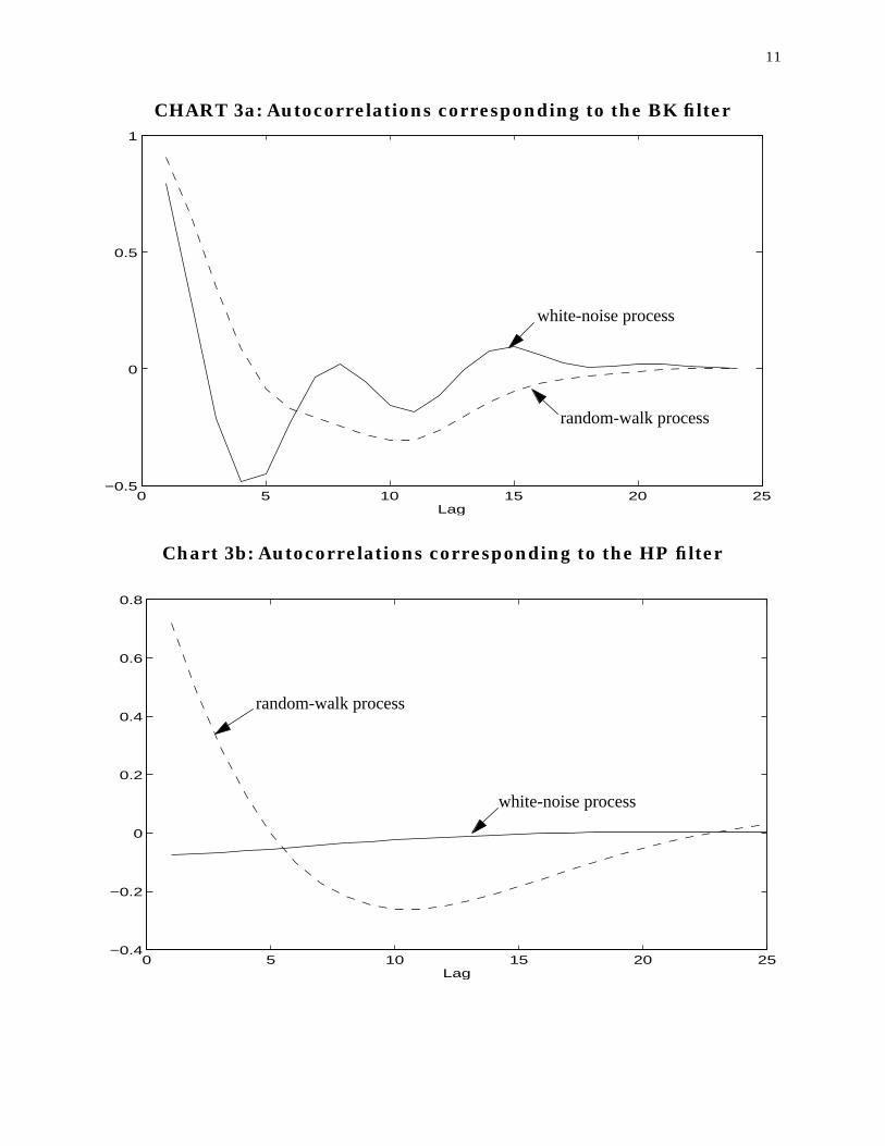
CHART 3a: Autocorrelations corresponding to the BK filter
Chart 3b: Autocorrelations corresponding to the HP filter
0 5 10 15 20 25−0.5
0
0.5
1
Lag
random-walk process
white-noise process
0 5 10 15 20 25−0.4
−0.2
0
0.2
0.4
0.6
0.8
Lag
white-noise process
random-walk process
12
Chart 3a shows the autocorrelation functions for the BK-filteredversion of a white-noise process and a random-walk process. In both cases, thecyclical component identified by the BK filter possesses strong positiveautocorrelations at shorter horizons. The result for the random walk is similar towhat Cogley and Nason (1995a) find for the HP filter (shown in Chart 3b).However, in contrast with the HP filter, the cyclical component identified by theBK filter displays strong dynamics for a white-noise process. One importantimplication of this result is that it precludes using the autocorrelation functionsresulting from this band-pass filter to evaluate the internal dynamic propagationmechanism of business-cycle models.
The spectrum of the cyclical component obtained via applying the BKfilter is
,
where is the squared gain of the BK filter and is the spectrum of. The squared gain is equal to , where denotes the Fourier
transform of at frequency . The pseudo-spectrum of is equal to
(sin2 )-r
for (see Priestley (1981), p. 597), where is the spectrum of the process, which is well defined since is stationary.
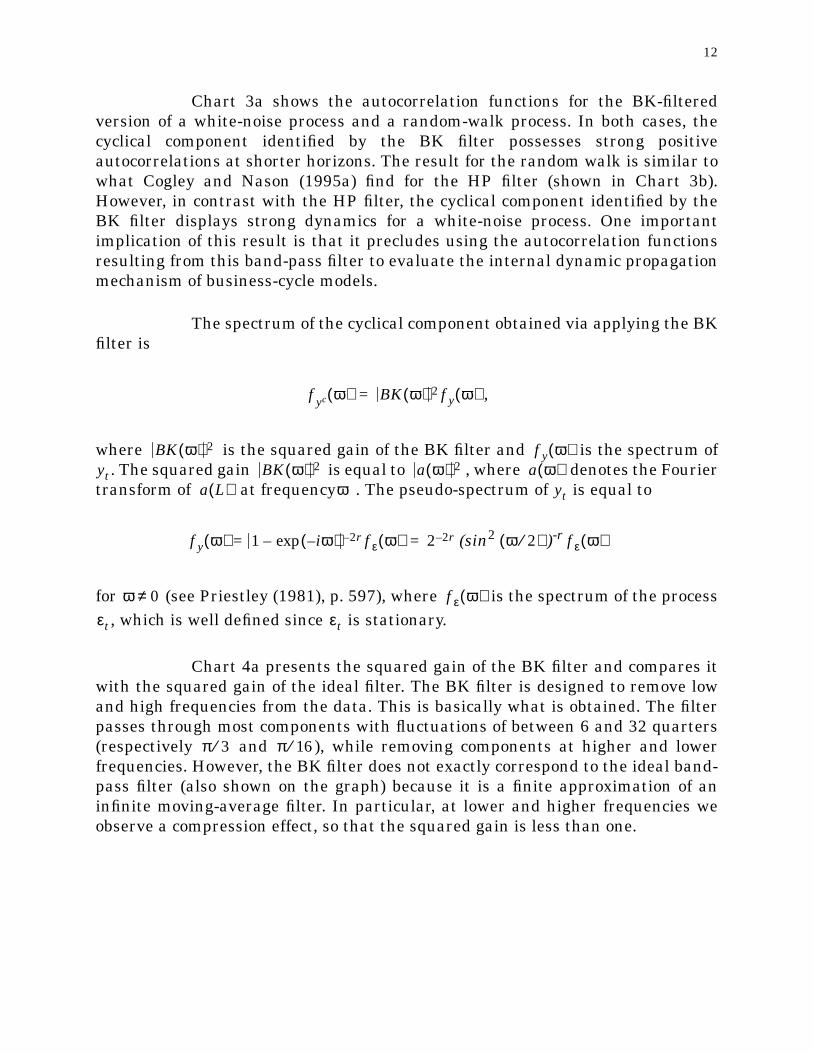
Chart 4a presents the squared gain of the BK filter and compares itwith the squared gain of the ideal filter. The BK filter is designed to remove lowand high frequencies from the data. This is basically what is obtained. The filterpasses through most components with fluctuations of between 6 and 32 quarters(respectively and ), while removing components at higher and lowerfrequencies. However, the BK filter does not exactly correspond to the ideal band-pass filter (also shown on the graph) because it is a finite approximation of aninfinite moving-average filter. In particular, at lower and higher frequencies weobserve a compression effect, so that the squared gain is less than one.
f yc ω( ) BK ω( ) 2 f y ω( )=
BK ω( ) 2 f y ω( )yt BK ω( ) 2 a ω( ) 2 a ω( )
a L( ) ω yt
f y ω( ) 1 iω–( )exp–= 2– r f ε ω( ) 2 2– r= ω 2⁄( ) f ε ω( )
ω 0≠ f ε ω( )εt εt
π 3⁄ π 16⁄
13
CHART 4a: Squared gain of the BK filter
As in Section 2.1, we now assume that r=1 and that is white noisewith variance equal to in equation (3). The spectrum of is then equal to 1 atall frequencies and the cyclical component obtained with the BK filter correspondsexactly to the squared gain of the BK filter as calculated by Cogley and Nason(1995a) and Harvey and Jaeger (1993) for the HP filter:
(sin2 )-1.
Chart 4b presents the pseudo-spectrum of and the spectrum of the cyclicalcomponent identified by the BK filter at business-cycle frequencies. Theconclusion once again depends on whether we are interested in retrieving thecomponent corresponding to business-cycle frequencies for the level of the series
or for the series in difference . In the latter case, as noted by Cogley andNason and by Harvey and Jaeger for the HP filter, the BK filter greatly amplifiesbusiness-cycle frequencies and creates spurious cycles when compared with theideal squared gain for the series in difference. For example, it amplifies by a factorof ten the variance of cycles with a periodicity of around 20 quarters ( ). Also,as in the case of the HP filter, business-cycle frequencies of the BK filtered seriesare less important than those of the original series in level and the cyclicalcomponent identified by the BK filter has a peak corresponding to a period of 20quarters (compared with 30 quarters in the case of the HP filter), which is absentfrom the spectrum of the level of the series .
0 0.05 0.1 0.15 0.2 0.25 0.30.2
0.4
0.6
0.8
1
1.2
fraction of pi(32 quarters) (6 quarters)
ideal filter
εt2π εt
BK ω( ) 2 1 iω–( )exp– 2– BK ω( ) 22 2–= ω 2⁄( )
yt
yt 1 L–( )yt
π 10⁄
yt

14
CHART 4b: Squared gain of the BK filter(Case of a random-walk process)
3. ABILITY OF THE FILTERS TO EXTRACT CYCLICAL PERIODICITIES
In this section, we examine how well the BK and HP filters capture the cyclicalcomponent of macroeconomic time series. Baxter and King’s (1995) first objectiveis to adequately extract a specified range of periodicities without altering theproperties of this extracted component. We use the same criteria to assess theperformance of the HP and BK filters. We show that when the peak of the spectral-density function of these series lies within business-cycle frequencies, these filtersprovide a good approximation of the corresponding cyclical component. If the peakis located at zero frequency, so that the bulk of the variance is located in lowfrequencies, those filters cannot identify the cyclical component adequately.
To show this, we consider the following data-generating process(DGP),
, (4)
where . A second-order autoregressive process is useful for our purpose
0.05 0.1 0.15 0.2 0.25 0.3 0.350
5
10
15
20
25
30
fraction of pi
spectrum of the series in levelsquared gain of the filter
squared gain of an ideal band-pass filter
yt φ1yt 1– φ2yt 2– εt+ +=
φ1 φ2 1<+

15
because its spectrum may have a peak at business-cycle frequencies or at zerofrequency. The spectrum of this process is equal to
and the location of its peak is given by
.
Thus, has a peak at frequencies other than zero for
and . (5)
Then has its peak at = cos-1 -- see Priestley (1981). Forother parameter values, the spectrum has a trough at non-zero frequencies if
and .
Charts 5 and 6 show the spectrum of autoregressive processes andthe spectrum of the cyclical component identified with the HP and BK filters.When the peak is located at zero frequency (i.e., most of the power of the series islocated at low frequencies) the spectrum of the cyclical component resulting fromthe application of both filters is very different from that of the original series,especially at lower frequencies (Chart 5). In particular, the HP and BK filtersinduce a peak at business-cycle frequencies even though it is absent from theoriginal series and they fail to capture a significant fraction of the variancecontained in the business-cycle frequencies. On the other hand, when the peak islocated at business-cycle frequencies, the spectrum of the cyclical componentidentified by HP and BK filtering matches fairly well the true spectrum at thesefrequencies (Chart 6). This result is robust for different sets of parameters and
. It is interesting to note that the BK filter does not perform as well as the HPfilter at frequencies corresponding to around 6 to 8 quarters cycles. Indeed, the BKfilter amplifies cycles of around 8 quarters but compresses those of around 6quarters. This results from the shape of the squared gain of the BK filter at thosefrequencies (see Chart 4a). The absence of a peak at business-cycle frequenciesdoes not imply that macroeconomic series do not feature business-cycles -- seeSargent (1987) for a discussion. In fact, while most macroeconomic series featurethe typical Granger shape, the growth rate of these series is often characterizedby a peak at the business-cycle frequencies. King and Watson (1996) call this “thetypical spectral shape of growth rates.”
f y ω( )σε
2
1 φ12 φ2
2 2φ1 1 φ2–( ) ωcos– 2φ2 2ωcos–+ +-----------------------------------------------------------------------------------------------------------=
σε2– f y ω( )2 2 ωsin( ) φ1 1 φ2–( ) 4φ2 ωcos+[ ]( )–
f y ω( )
φ2 0< φ1 1 φ2–( )–
4φ2---------------------------- 1<
f y ω( ) ω φ1 1 φ2–( ) 4φ2⁄–( )
φ2 0> φ1 1 φ2–( ) 4φ2⁄ 1<
φ1φ2

16
CHART 5: Series having the typical Granger shape(AR(2) coefficients: 1.26 -0.31)
CHART 6: Series with a peak at business-cycle frequencies(AR(2) coefficients: 1.26 -0.78)
0.05 0.1 0.15 0.2 0.25 0.3 0.350
0.02
0.04
0.06
0.08
0.1
0.12
0.14
fraction of pi
unfiltered
HP-filtered
BK-filtered
(32 quarters) (6 quarters)
0.05 0.1 0.15 0.2 0.25 0.3 0.350
0.01
0.02
0.03
0.04
0.05
0.06
0.07
0.08
fraction of pi
unfiltered
HP-filtered
BK-filtered
(32 quarters) (6 quarters)

17
To examine this question in more detail, we perform the followingexercise. First, we set a DGP by a choice of for the second-orderautoregressive process of equation (4). Second, we extract the correspondingcyclical component with the HP or BK filters. Third, we search among second-order autoregressive processes for the parameters and that minimize thedistance, at business-cycle frequencies, between the spectrum of this process andthe spectrum of the HP- or BK-filtered true second-order autoregressive processes.The problem is the following
,
where , , is the spectrum of the filtered DGP (where is the vector of true values for the parameters and ), and is the
spectrum of the evaluated autoregressive process. Thus, in the case where the HPand BK filters extract adequately the range of periodicities corresponding tofluctuations of between 6 and 32 quarters (respectively, and ),
will be equal to the true vector . Otherwise, the filter will extract a cyclicalcomponent corresponding to a second-order autoregressive process differing fromthe true one.
Table 1 presents our results for a DGP where the autoregressiveparameter of order 1 is set at 1.20 while the parameter of order 2 is allowed to vary.Using the restrictions implied by (5), the peak of the spectrum lies withinbusiness-cycle frequencies when .43. Although we report results only forthe HP filter, these are almost identical to those obtained with the BK filter.7
Results from this exercise corroborate those obtained from visual inspection. Thesecond-order autoregressive process which minimizes the distance between itsspectrum at business-cycle frequencies and that of the business-cycle componentidentified by the HP and BK filters for the true process is very different from thetrue second-order autoregressive process when the peak of the DGP is located atzero frequency. When the peak is located at business-cycle frequencies, theresulting second-order autoregressive process is close to the true second-orderautoregressive process.
7. These results are robust to the use of alternative values for , so that the restrictionsare respected.
θ φ1 φ2,( )=
φ1 φ2
θ min Syf ω θ0;( ) Sy ω θ;( )–( )2 ωdω1
ω2
∫arg=
ω1 π 16⁄= ω2 π 3⁄= Syf ω θ0;( )θ0 φ1 φ2 Sy ω θ;( )
ω π 3⁄= ω π 16⁄=θ θ0
φ2 0–<
θ0

18
The spectrum of the level of macroeconomic time series typically lookslike that of the unfiltered series shown on Chart 5. The spectrum’s peak is locatedat zero frequency and the bulk of its variance is located in the low frequencies.This is what is called Granger’s typical shape. Charts 7, 8, 9 and 10 display theestimated spectra of U.S. real GDP, real consumption, consumer price inflation,and the unemployment rate, as well as the spectra of the filtered counterparts tothese series.8 It is clear that the filters perform badly in terms of capturingbusiness-cycle frequencies in these cases.
8. We use a parametric estimator of the spectrum. An autoregressive process was fittedand the order of that process was determined on the basis of the Akaike criteria.
TABLE 1: Fitted values for the HP filter
DGP ( ) HP ( )
1.20 -0.25 -0.09 0.72
1.20 -0.30 0.12 0.40
1.20 -0.35 0.48 -0.15
1.20 -0.40 0.87 -0.20
1.20 -0.45 1.09 -0.41
1.20 -0.50 1.16 -0.50
1.20 -0.55 1.19 -0.56
1.20 -0.60 1.20 -0.61
1.20 -0.65 1.20 -0.66
1.20 -0.70 1.20 -0.70
1.20 -0.75 1.20 -0.75
1.20 -0.80 1.20 -0.80
θ0 θ
φ1 φ2 φ1 φ2
19
The intuition behind this result is simple. Charts 1 and 4a (Section 2)show that the gains of the HP and BK filters at low business-cycle frequencies aresignificantly smaller than that of the ideal filter. Indeed, the squared gain of theBK filter is 0.34 at frequencies corresponding to 32-quarter cycles, while that ofthe HP filter is 0.49. In the case of the HP filter, the squared gain does not reach0.95 before frequency (cycles of 16 quarters). The problem is that a largefraction of the power of typical macroeconomic time series at business-cyclefrequencies is concentrated in the band where the squared gains of HP and BKfilters differ from that of an ideal filter. Also, the shape of the squared gain of thosefilters when applied to typical macroeconomic time series induces a peak in thespectrum of the cyclical component that is absent from the original series. In short,applying the HP and BK filters to series dominated by low frequencies results inthe extraction of a cyclical component that does not capture an important fractionof the variance contained in business-cycle frequencies of the original series andthat induces spurious dynamic properties.
One could argue that macroeconomic time series are really made of apermanent component and a cyclical component, so that the peak of the spectrumof the series would be at zero frequency while the peak of the spectrum of thecyclical component would be at business-cycle frequencies. For example, thepermanent component could be driven by a random-walk technological processwith drift, while transitory monetary- or fiscal-policy shocks, among others, wouldgenerate the cyclical component with a peak in its spectrum at business-cyclefrequencies. If this is true, then the HP and BK filters might be able to adequatelycapture the cyclical component. We examine this issue in the next section.
π 8⁄

20
CHART 7: Spectrum of the logarithm of U.S. real GDP
CHART 8: Spectrum of the logarithm of U.S. real consumption
0 0.05 0.1 0.15 0.2 0.25 0.3 0.350
0.05
0.1
0.15
0.2
0.25
0.3
0.35
fraction of pi
unfiltered
BK-filtered
HP-filtered
(32 quarters) (6 quarters)
0 0.05 0.1 0.15 0.2 0.25 0.3 0.350
0.1
0.2
0.3
0.4
0.5
0.6
0.7
0.8
fraction of pi
unfiltered
HP-filteredBK-filtered
(32 quarters) (6 quarters)

21
CHART 9: Spectrum of U.S. consumer price inflation
CHART 10: Spectrum of U.S. unemployment rate
0 0.05 0.1 0.15 0.2 0.25 0.3 0.350
500
1000
1500
2000
2500
3000
3500
4000
fraction of pi
BK-filteredHP-filtered
unfiltered
(32 quarters) (6 quarters)
0 0.05 0.1 0.15 0.2 0.25 0.3 0.350
100
200
300
400
500
600
fraction of pi
unfiltered
HP-filtered
BK-filtered
(32 quarters) (6 quarters)
22
4. A SIMULATION STUDY
Consider the following DGP:
, (6)
where
and
, .
Equation (6) defines as the sum of a permanent component, , which in thiscase corresponds to a random walk, and a cyclical component, .9 The dynamicsof the cyclical component are specified as a second order autoregressive process sothat the peak of the spectrum could be at zero frequency or at business-cyclefrequencies. We assume that and are uncorrelated.
Data are generated from equation (6) with set at 1.2 and differentvalues for to control the location of the peak in the spectrum of the cyclicalcomponent. We also vary the standard-error ratio for the disturbances tochange the relative importance of each component. We follow the standardpractice of giving the value 1,600 to , the HP filter smoothness parameter. Wealso follow Baxter and King’s suggestion of dropping 12 observations at thebeginning and at the end of the sample. The resulting series contains 150observations, a standard size for quarterly macroeconomic data. The number ofreplications is 500.
The performance of the HP and BK filters is assessed by comparingthe autocorrelation function of the cyclical component of the true process to withthat obtained from the filtered data. We also calculate the correlation between thetrue cyclical component and the filtered cyclical component and report theirrelative standard deviations ( ). Table 2 presents the results for the HP filter
9. This is Watson’s (1986) specification for U.S. real GDP.
yt µt ct+=
µt µt 1– εt+=
ct φ1ct 1– φ2ct 2– η+ t+=
εt NID 0 σε2,( )∼ ηt NID 0 ση
2,( )∼
yt µtct
εt ut
φ1φ2
σε ση⁄
λ
σc σc⁄

23
and Table 3 those for the BK filter.
Table 2 shows that the HP filter performs particularly poorly whenthere is an important permanent component. Indeed, for high ratios, inmost cases the correlation between the true and the filtered components is notsignificantly different from zero. The estimated autocorrelation function isinvariant to the change in the cyclical component in these cases (the values of thetrue autocorrelation functions are given in parentheses in the tables). When theratio is equal to 0.5 or 1 and the peak of the cyclical component is locatedat zero frequency ( .43), the dynamic properties of the true and the filteredcyclical components are significantly different, as indicated by the estimatedparameter values. In general, the HP filter adequately characterizes the seriesdynamics when the peak of the spectrum is at business-cycle frequencies and theratio is small. However, even when the ratio of standard deviations is equalto 0.01 (i.e. the permanent component is almost absent), the filter performs poorlywhen the peak of the spectrum of the cyclical component is at zero frequency.Indeed, for .25, the dynamic properties of the filtered component differsignificantly from those of the true cyclical component, the correlation is onlyequal to 0.66, and the standard deviation of the filtered cyclical component is halfthat of the true cyclical component.
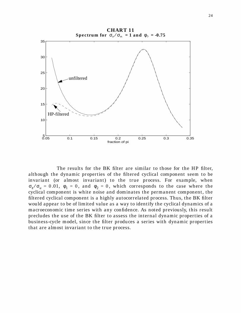
It is interesting to note that the HP filter does relatively well whenthe ratio is equal to 1, 0.5, or 0.01 and the spectrum of the original serieshas a peak at zero frequency and at business-cycle frequencies (i.e. the latterfrequencies contains a significant part of the variance of the series). This isreflected in Chart 11, which shows the spectrum for the case where = 1 and
= -0.75. Consequently, the conditions required to adequately identify thecyclical component with the HP filter can be expressed in the following way: thespectrum of the original series must have a peak located at business-cyclefrequencies, which must account for an important part of the variance of theseries. If the variance of the series is dominated by low frequencies, which is thecase for most macroeconomic series in levels, the HP filter does a poor job ofextracting the cyclical component.
σε ση⁄
σε ση⁄φ2 0–>
σε ση⁄
φ2 0–=
σε ση⁄
σε ση⁄φ2
24
CHART 11Spectrum for = 1 and = -0.75
The results for the BK filter are similar to those for the HP filter,although the dynamic properties of the filtered cyclical component seem to beinvariant (or almost invariant) to the true process. For example, when
.01, , and , which corresponds to the case where thecyclical component is white noise and dominates the permanent component, thefiltered cyclical component is a highly autocorrelated process. Thus, the BK filterwould appear to be of limited value as a way to identify the cyclical dynamics of amacroeconomic time series with any confidence. As noted previously, this resultprecludes the use of the BK filter to assess the internal dynamic properties of abusiness-cycle model, since the filter produces a series with dynamic propertiesthat are almost invariant to the true process.
σε ση⁄ φ2
0.05 0.1 0.15 0.2 0.25 0.3 0.355
10
15
20
25
30
35
fraction of pi
unfiltered
HP-filtered
σε σu⁄ 0= φ1 0= φ2 0=

25
TABLE 2: Simulation results for the HP filter
DGP Estimated values
Autocorrelationscorrelation
1 2 3
10 0 0 .71[0](.59,.80)
.46[0](.30,.60)
.26[0](.08,.43)
.08(-.07,.21)
12.96(10.57,15.90)
10 1.2 -.25 .71[.96](.61,.80)
.47[.90](.31,.61)
.27[.84](.08,.44)
.08(-.11,.28)
4.19(2.77,6.01)
10 1.2 -.40 .71[.86](.60,.80)
.46[.63](.30,.60)
.26[.41](.08,.44)
.13(-.12,.36)
6.34(4.82,8.07)
10 1.2 -.55 .71[.77](.60,.80)
.46[.38](.29,.60)
.26[.03](.06,.43)
.14(-.08,.33)
6.93(5.36,8.70)
10 1.2 -.75 .71[.69](.60,.78)
.46[.27](.30,.59)
.25[-.19](.07,.41)
.15(-.01,.31)
6.37(4.79,7.95)
5 0 0 .69[0](.58,.78)
.45[0](.30,.58)
.26[0](.09,.41)
.15(.02,.27)
6.50(5.28,7.85)
5 1.2 -.25 .71[.96](.61,.80)
.46[.90](.32,.61)
.26[.84](.08,.43)
.16(-.01,.36)
2.11(1.43,3.04)
5 1.2 -.40 .72[.86](.61,.80)
.46[.63](.31,.60)
.25[.41](.08,.42)
.23(-.01,.45)
3.26(2.47,4.15)
5 1.2 -.55 .71[.77](.61,.80)
.46[.38](.30,.59)
.24[.03](.06,.41)
.24(.01,.44)
3.60(2.83,4.52)
5 1.2 -.75 .70[.69](.61,.79)
.43[.27](.26,.57)
.20[-.19](.00,.38)
.29(.11,.44)
3.30(2.53,4.17)
1 0 0 .43[0](.27,.57)
.28[0](.11,.42)
.20[0](-.02,.31)
.59(.49,.70)
1.61(1.41,1.85)
1 1.2 -.25 .76[.96](.67,.83)
.51[.90](.37,.62)
.29[.84](.11,.44)
.51(.33,.68)
.66(.44,.91)
1 1.2 -.40 .75[.86](.67,.81)
.44[.63](.28,.55)
.16[.41](-.03,.33)
.71(.56,.82)
1.02(.83,1.22)
1 1.2 -.55 .72[.77](.66,.78)
.34[.38](.21,.47)
.01[.03](-.17,.19)
.76(.56,.82)
1.15(.83,1.22)
1 1.2 -.75 .68[.69](.63,.72)
.15[.27](.04,.27)
-.27[-.19](-.44,.10)
.83(.75,.89)
1.16(1.04,1.29)
.5 0 0 .16[0](.01,.32)
.10[0](-.04,0.24)
.04[0](-.10,.18)
.82(.75,.88)
1.16(1.07,1.27)
.5 1.2 -.25 .79[.96](.71,.85)
.53[.90](.38,.65)
.30[.84](.11,.46)
.61(.41,.79)
.55(.37,.76)
.5 1.2 -.40 .77[.86](.69,.81)
.43[.63](.29,.54)
.13[.41](-.05,.29)
.84(.73,.92)
.87(.74,.99)
.5 1.2 -.55 .72[.77](.67,.78)
.28[.38](.17,.39)
-.10[.03](-.25,.06)
.89(.83,.94)
.98(.89,1.07)
.5 1.2 -.75 .67[.69](.63,.71)
.07[.27](-.03,.18)
-.42[-.19](-.57,-.27)
.94(.90,.96)
1.02(.97,1.08)
σε ση⁄ φ1 φ2 σc σc⁄
(continued)

26
TABLE 2: (Continued)
DGP Estimated values
Autocorrelationscorrelation
1 2 3
.01 0 0 -.08[0](-.21,.06)
-.06[0](-.21,.06)
-.06[0](-.19,.06)
.98(.96,.99)
.97(.94,.99)
.01 1.2 -.25 .80[.96](.72,.86)
.54[.90](.38,.67)
.30[.84](.11,.48)
.66(.45,.83)
.51(.34,.69)
.01 1.2 -.40 .78[.86](.72,.83)
.43[.63](.30,.55)
12[.41](-.05,.28)
.90(.82,.96)
.81(.71,.90)
.01 1.2 -.55 .73[.77](.67,.77)
.26[.38](.15,.37)
-.14[.03](-.30,.01)
.96(.91,.99)
.92(.86,.96)
.01 1.2 -.75 .67[.69](.62,.71)
.02[.27](-.08,.13)
-.50[-.19](-.61,-.35)
.99(.97,1.0)
.97(.95,.99)
TABLE 3: Simulation results for the BK filter
DGP Estimated values
Autocorrelationscorrelation
1 2 3
10 0 0 .90[0](.87,.93)
.65[0](.52,.75)
.33[0](.13,.51)
.03(-.11,.16)
11.55(9.05,14.38)
10 1.2 -.25 .90[.96](.87,.93)
.65[.90](.55,.74)
.34[.84](.17,.49)
.08(-.13,.32)
3.71(2.34,5.45)
10 1.2 -.40 .90[.86](.87,.93)
.64[.63](.54,.73)
.33[.41](.16,.48)
.11(-.16,.36)
5.67(4.19,7.18)
10 1.2 -.55 .90[.77](.87,.93)
.64[.38](.53,.73)
.33[.03](.14,.48)
.12(-.12,.33)
6.23(4.71,7.93)
10 1.2 -.75 .90[.69](.86,.92)
.63[.27](.52,.73)
.31[-.19](.13,.48)
.16(-.04,.36)
5.69(4,37,7.16)
5 0 0 .90[0](.87,.90)
.64[0](.53,.73)
.33[0](.14,.49)
.05(-.09,.20)
5.80(4.54,7.16)
5 1.2 -.25 .90[.96](.87,.93)
.65[.90](.54,.73)
.34[.84](.16,.49)
.17(-.05,.38)
1.94(1.25,2.74)
5 1.2 -.40 .90[.86](.87,.93)
.64[.63](.53,.74)
.32[.41](.14,.49)
.23(-.03,.47)
2.93(2.15,3.76)
5 1.2 -.55 .89[.77](.87,.92)
.62[.38](.52,.72)
.30[.03](.12,.46)
.26(.03,.46)
3.19(2.45,3.98)
5 1.2 -.75 .88[.69](.85,.92)
.60[.27](.47,.70)
.26[-.19](.06,.44)
.28(.09,.45)
2.97(2.24,3.77)
1 0 0 .89[0](.85,.92)
.61[0](.48,.71)
.27[0](.06,.45)
.19(.05,.32)
1.21(.96,1.43)
1 1.2 -.25 .90[.96](.87,.93)
.65[.90](.53,.74)
.34[.84](.15,.50)
.53(.36,.71)
.60(.39,.84)
σε ση⁄ φ1 φ2 σc σc⁄
σε ση⁄ φ1 φ2 σc σc⁄
(continued)
27
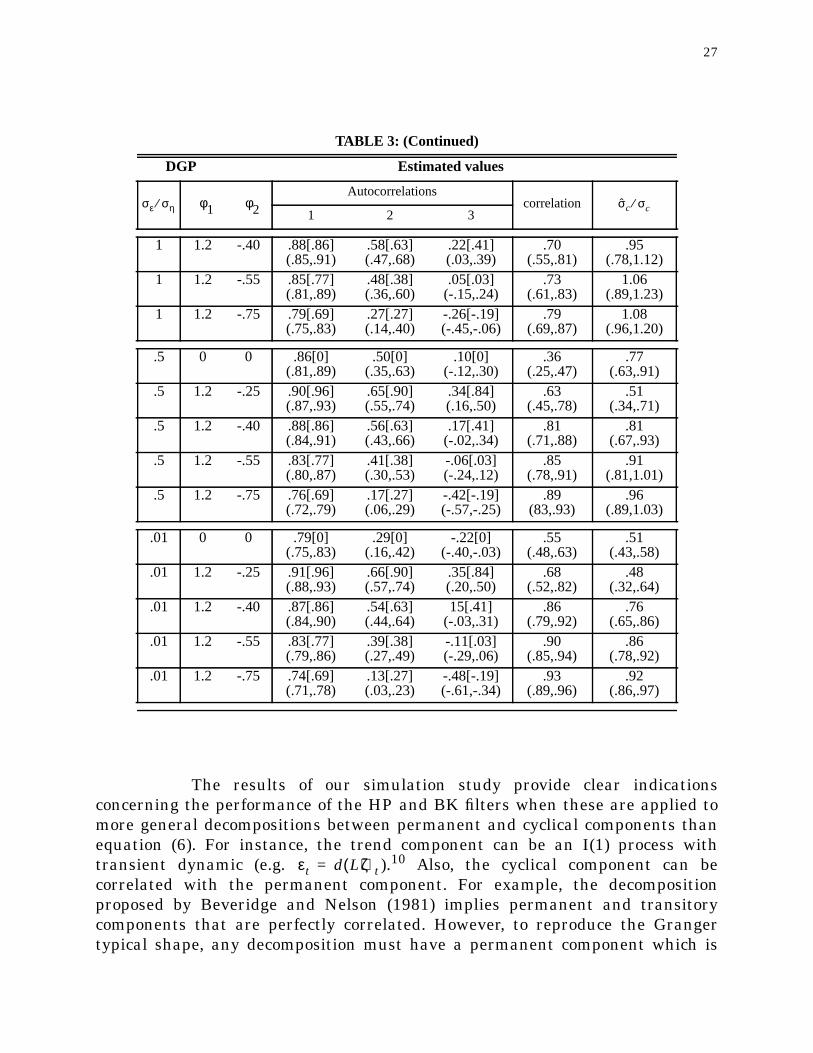
The results of our simulation study provide clear indicationsconcerning the performance of the HP and BK filters when these are applied tomore general decompositions between permanent and cyclical components thanequation (6). For instance, the trend component can be an I(1) process withtransient dynamic (e.g. ).10 Also, the cyclical component can becorrelated with the permanent component. For example, the decompositionproposed by Beveridge and Nelson (1981) implies permanent and transitorycomponents that are perfectly correlated. However, to reproduce the Grangertypical shape, any decomposition must have a permanent component which is
TABLE 3: (Continued)
DGP Estimated values
Autocorrelationscorrelation
1 2 3
1 1.2 -.40 .88[.86](.85,.91)
.58[.63](.47,.68)
.22[.41](.03,.39)
.70(.55,.81)
.95(.78,1.12)
1 1.2 -.55 .85[.77](.81,.89)
.48[.38](.36,.60)
.05[.03](-.15,.24)
.73(.61,.83)
1.06(.89,1.23)
1 1.2 -.75 .79[.69](.75,.83)
.27[.27](.14,.40)
-.26[-.19](-.45,-.06)
.79(.69,.87)
1.08(.96,1.20)
.5 0 0 .86[0](.81,.89)
.50[0](.35,.63)
.10[0](-.12,.30)
.36(.25,.47)
.77(.63,.91)
.5 1.2 -.25 .90[.96](.87,.93)
.65[.90](.55,.74)
.34[.84](.16,.50)
.63(.45,.78)
.51(.34,.71)
.5 1.2 -.40 .88[.86](.84,.91)
.56[.63](.43,.66)
.17[.41](-.02,.34)
.81(.71,.88)
.81(.67,.93)
.5 1.2 -.55 .83[.77](.80,.87)
.41[.38](.30,.53)
-.06[.03](-.24,.12)
.85(.78,.91)
.91(.81,1.01)
.5 1.2 -.75 .76[.69](.72,.79)
.17[.27](.06,.29)
-.42[-.19](-.57,-.25)
.89(83,.93)
.96(.89,1.03)
.01 0 0 .79[0](.75,.83)
.29[0](.16,.42)
-.22[0](-.40,-.03)
.55(.48,.63)
.51(.43,.58)
.01 1.2 -.25 .91[.96](.88,.93)
.66[.90](.57,.74)
.35[.84](.20,.50)
.68(.52,.82)
.48(.32,.64)
.01 1.2 -.40 .87[.86](.84,.90)
.54[.63](.44,.64)
15[.41](-.03,.31)
.86(.79,.92)
.76(.65,.86)
.01 1.2 -.55 .83[.77](.79,.86)
.39[.38](.27,.49)
-.11[.03](-.29,.06)
.90(.85,.94)
.86(.78,.92)
.01 1.2 -.75 .74[.69](.71,.78)
.13[.27](.03,.23)
-.48[-.19](-.61,-.34)
.93(.89,.96)
.92(.86,.97)
σε ση⁄ φ1 φ2 σc σc⁄
εt d L( )ζt=

28
important relative to the cyclical component or a cyclical component dominated bylow frequencies. In both cases, the HP and BK filters provide a distorted cyclicalcomponent.11
5. COMPARISON WITH OTHER APPROACHES
In this section, we compare the cyclical component obtained using the HP and BKfilters with those of other approaches. Watson (1986) proposes an unobservedstochastic trend decomposition into permanent and cyclical components. Hismodel for U.S. real GDP corresponds to equation (6) presented in the previoussection.
It would be interesting to see whether the HP or BK filter is able tocapture the cyclical component of the above DGP. Using Kuttner’s (1994)estimates ( = 1.44, = - 0.47, = 0.0052, and = 0.0069),12 we simulateddata on the basis of this DGP, filtered it, and compared the dynamic properties andthe correlation of the true and the filtered components. The results are shown inTable 4. Both the HP and BK filters produce cyclical components with dynamicproperties significantly different from the true one. Notably, the cyclicalcomponents identified by both filters are much less persistent than the true one.Also, the correlation is rather small. These results are not surprising given thatthe spectrum of the cyclical component has its peak at zero frequency and the bulkof the variance is located in the low frequencies.
10. Lippi and Reichlin (1994) argue that modeling the trend component in real GNP as arandom walk is inconsistent with the standard view concerning the diffusion processof technological shocks. Blanchard and Quah (1989) and King, Plosser, Stock andWatson (1991) used a multivariate representation to obtain a trend component havingan impulse function with a short-run impact smaller than the long-run impact. Thus,the effect of the permanent shock gradually increases to its long-run impact.
11. The results of complementary similations with different processes are available onrequest. For brevity these are not shown here.
12. We chose Kuttner’s estimates because he uses a larger sample than Watson. The useof Watson’s estimates would not change our conclusions, however.
φ1 φ2 σε2 ση
2

29
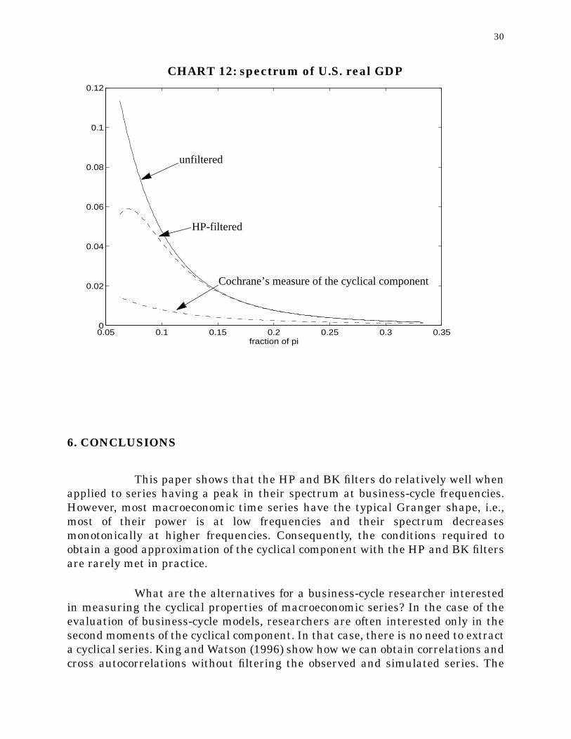
Cochrane (1994) proposes a simple detrending method for outputbased on the permanent-income hypothesis. This implies (for a constant realinterest rate) that consumption is a random walk with drift that is cointegratedwith total income. Thus, any fluctuations in GDP with unchanged consumptionmust be transitory. Cochrane uses these assumptions to decompose U.S. real GDPinto permanent and transitory components. Chart 12 presents the spectra for U.S.real GDP, for the same series when it is HP-filtered, and for Cochrane’s cyclicalcomponent.
Using Cochrane’s measure for comparison, the HP cyclical componentgreatly amplifies business-cycle frequencies. Also, while the peak of the spectrumof the HP-filtered cyclical component is located at business-cycle frequencies, thepeak of Cochrane’s measure is at zero frequency. The correlation between the twocyclical components is 0.57. To the extent that Cochrane’s method provides a goodapproximation of the cyclical component of U.S. real GDP, the HP-filtered measureappears inadequate.
TABLE 4
AutocorrelationsCorrelation
1 2 3
Theoretical values 0.98 0.94 0.89 --
BK filter 0.92(0.89-0.94)
0.70(0.60-0.78)
0.42(0.25-0.56)
0.47(0.30-0.67)
HP filter 0.84(0.78-0.89)
0.61(0.48-0.73)
0.38(0.20-0.54)
0.56(0.35-0.76)
30
CHART 12: spectrum of U.S. real GDP
6. CONCLUSIONS
This paper shows that the HP and BK filters do relatively well whenapplied to series having a peak in their spectrum at business-cycle frequencies.However, most macroeconomic time series have the typical Granger shape, i.e.,most of their power is at low frequencies and their spectrum decreasesmonotonically at higher frequencies. Consequently, the conditions required toobtain a good approximation of the cyclical component with the HP and BK filtersare rarely met in practice.
What are the alternatives for a business-cycle researcher interestedin measuring the cyclical properties of macroeconomic series? In the case of theevaluation of business-cycle models, researchers are often interested only in thesecond moments of the cyclical component. In that case, there is no need to extracta cyclical series. King and Watson (1996) show how we can obtain correlations andcross autocorrelations without filtering the observed and simulated series. The
0.05 0.1 0.15 0.2 0.25 0.3 0.350
0.02
0.04
0.06
0.08
0.1
0.12
fraction of pi
unfiltered
HP-filtered
Cochrane’s measure of the cyclical component
31
strategy consists in calculating these moments from the estimated spectraldensity matrix for business-cycle frequencies. We can obtain an estimator of thespectral density matrix with a parametric estimator, such as that used by Kingand Watson, or a non parametric estimator. The cyclical component can also beobtained in a univariate or a multivariate representation with the Beveridge-Nelson (1981) decomposition. Economic theory also provides alternative methodsof detrending. For example, Cochrane’s method (1994) based on the permanentincome theory or the Blanchard and Quah (1989) structural decomposition can beused.13 The authors are currently investigating the properties of these alternativemethodologies.
13. Cogley (1996) compares the HP and BK filters with the univariate Beveridge-Nelsondecomposition and Cochrane’s method using a R.B.C. model with different exogenousprocesses.
32
REFERENCES
Baxter, M. 1994. “Real Exchange Rates and Real Interest Differentials: Have weMissed the Business-Cycle Relationship?” Journal of Monetary Economics33: 5-37.
Baxter, M. and R. G. King. 1995. “Measuring Business-cycles: Approximate Band-Pass Filters for Economic Time Series.” Working Paper No. 5022. NationalBureau of Economic Research.
Beveridge, S. and C. R. Nelson (1981). “A New Approach to the Decomposition ofEconomic Time Series into Permanent and Transitory Components withParticular Attention to Measurement of the Business Cycle.” Journal ofMonetary Economics 7: 151-74.
Blanchard, O. J. and D. Quah. 1989. “The Dynamic Effect of Aggregate Demandand Supply Disturbances.” American Economic Review 79: 655-73.
Burns, A. M. and W. C. Mitchell. 1946. Measuring Business-Cycles.
Cecchetti S. G. and A. K. Kashyap. 1995. “International Cycles.” Working PaperNo. 5310. National Bureau of Economic Research.
Cochrane, J. H. 1994. “Permanent and Transitory Components of GNP and StockPrices.” Quarterly Journal of Economics 61: 241-65.
Cogley, T. 1996. “Evaluating Non-Structural Measures of the Business Cycle.”Draft Paper. Federal Reserve Bank of San Francisco.
Cogley, T. and J. Nason. 1995a. “Effects of the Hodrick-Prescott filter on Trend andDifference Stationary Time Series: Implications for Business-CycleResearch.” Journal of Economic Dynamics and Control 19: 253-78.
Cogley, T. and J. Nason. 1995b. “Output Dynamics in Real Business Cycle Models.”American Economic Review 85: 492-511.
Gouriéroux, C. and M. Monfort. 1995. Séries Temporelles et Modèles Dynamiques.Economica.
Granger, C. W. J. 1966. “The Typical Spectral Shape of an Economic Variable.”Econometrica 37: 424-38.
Harvey, A. C. and A. Jaeger. 1993. “Detrending, Stylized Facts and the Business-Cycle.” Journal of Applied Econometrics 8: 231-47.
Hasler, J., P. Lundvik, T. Persson, and P. Soderlind. 1994. “The Swedish Business-Cycle: Stylized Facts Over 130 Years.” In Measuring and InterpretingBusiness-Cycles, ed. V. Berstrom and A. Vredin. Oxford: Clarendon Press,pp. 7-108.
Hodrick, R. J. and E. Prescott. 1980. “Post-war U. S. Business-Cycles: AnEmpirical Investigation.” Working Paper. Carnegie-Mellon University.
33
Howrey, E.P. 1968. “A Spectral Analysis of the Long-swing Hypothesis.”International Economic Review 2: 228-60.
King, R. G., C. I. Plosser, and S. Rebelo. 1988. “Production, Growth, and BusinessCycles, II. New Directions.” Journal of Monetary Economics 21: 309-42.
King, R. G., C. I. Plosser, J. H. Stock, and M. W. Watson. 1991. “Stochastic Trendsand Economic Fluctuations.” American Economic Review 81 (September):819-40.
King, R. G. and S. Rebelo. 1993. “Low Frequency Filtering and Real Business-Cycles.” Journal of Economic Dynamics and Control 17: 207-31.
King, R. G., J. H. Stock and M. Watson. 1995. “Temporal Instability of theUnemployment-Inflation Relationship.” Economic Perspectives. FederalReserve Bank of Chicago. Vol. 19, pp. 753-95.
King, R. G., M. Watson. 1996. “Money, Prices, Interest Rates and the Business-Cycle.” Forthcoming in the Review of Economics and Statistics.
Kuttner, K. N. 1994. “Estimating Potential Output as a Latent Variable.” Journalof Business and Economic Statistics 12: 361-68.
Laxton, D. and R. Tetlow. 1992. A Simple Multivariate Filter for the Measurementof Potential Output. Technical Report No. 59. Ottawa: Bank of Canada.
Lippi, M. and Reichlin (1994). “Diffusion of Technical Change and theDecomposition of Output into Trend and Cycle.” Review of Economic Studies61: 19-30.
Nelson, C. R. and H. Kang. 1981. “Spurious Periodicity in InappropriatelyDetrended Time Series.” Econometrica 49: 741-51.
Nelson, C. R. and C. Plosser. 1982. “Trends and Ransom Walks in MacroeconomicTime Series.” Journal of Monetary Economics 10: 139-67.
Osborn, D. R. 1995. “Moving Average Detrending and the Analysis of Business-Cycles.” Forthcoming in Oxford Bulletin of Economics and Statistics.
Priestly, M. 1981. Spectral Analysis and Time Series. Academic Press.
Quah, D. 1992. “The Relative Importance of Permanent and TransitoryComponents: Identification and Some Theoretical Bounds.” Econometrica60: 107-18.
Rotemberg J. and M. Woodford. 1996. Real Business Cycle Models and theForecastable Movements in Output, Hours, and Consumption. TheAmerican Economic Review 86: 71-89.
Sargent, T. J. 1987. Macroeconomic Theory. Academic Press.
Singleton, K. 1988. “Econometric Issues in the Analysis of Equilibrium Business-Cycle Models.” Journal of Monetary Economics 21: 361-86.
Slutzky, E. 1937. “The Summation of Random Causes as the Source of CyclicProcesses.” Econometrica: 5. 105-46.
34
Van Norden, S. 1995. “Why is it so Hard to Measure the Current Output Gap?”Mimeo. Bank of Canada.
Watson, M. W. 1986. “Univariate Detrending Methods with Stochastic Trends.”Journal of Monetary Economics 18: 49-75.
Watson, M. W. 1988. “Measures of Fit for Calibrated Models.” Journal of PoliticalEconomy 101: 1011-41.