DI

SC

US

SI

ON

P

AP

ER

S

ER

IE

S

Forschungsinstitut zur Zukunft der ArbeitInstitute for the Study of Labor

Do SBA Loans Create Jobs?

IZA DP No. 7544

August 2013

J. David BrownJohn S. Earle

Do SBA Loans Create Jobs?

J. David Brown U.S. Census Bureau

and IZA

John S. Earle George Mason University,

CEU and IZA

Discussion Paper No. 7544 August 2013

IZA

P.O. Box 7240 53072 Bonn

Germany

Phone: +49-228-3894-0 Fax: +49-228-3894-180

E-mail: iza@iza.org

Any opinions expressed here are those of the author(s) and not those of IZA. Research published in this series may include views on policy, but the institute itself takes no institutional policy positions. The IZA research network is committed to the IZA Guiding Principles of Research Integrity. The Institute for the Study of Labor (IZA) in Bonn is a local and virtual international research center and a place of communication between science, politics and business. IZA is an independent nonprofit organization supported by Deutsche Post Foundation. The center is associated with the University of Bonn and offers a stimulating research environment through its international network, workshops and conferences, data service, project support, research visits and doctoral program. IZA engages in (i) original and internationally competitive research in all fields of labor economics, (ii) development of policy concepts, and (iii) dissemination of research results and concepts to the interested public. IZA Discussion Papers often represent preliminary work and are circulated to encourage discussion. Citation of such a paper should account for its provisional character. A revised version may be available directly from the author.

IZA Discussion Paper No. 7544 August 2013

ABSTRACT

Do SBA Loans Create Jobs?* Small Business Administration (SBA) loans have long been one of the most significant policy interventions in the U.S. affecting firm behavior, but little is known about their outcomes. This paper estimates the effects on employment using a list of all SBA loans linked to annual data on all U.S. employers from 1976 to 2010. Our methods combine firm fixed-effect regressions with matching on exact firm age, industry, year, and pre-loan size, and on propensity scores as a function of four years of employment history and other variables. The results imply positive average effects on loan recipient employment of about 25 percent, or 3 jobs at the mean. Including loan amount, we find little or no impact of loan receipt per se, but an increase of about 5.4 jobs for each million dollars of loans. Similar results for high-growth counties and industries suggest the estimates are not driven by differential demand conditions across firms. Exploiting variation in the distance of controls from recipient firms, we find only very small displacement effects. In all these cases, the results pass “placebo” and “pre-program” specification tests. Other specifications using only matching or only regression imply somewhat higher effects, but they fail these tests. The estimates facilitate calculations of total job creation by the SBA and of the cost per job created. JEL Classification: D04, G21, G28, H32, H81, J23, L52 Keywords: small business finance, entrepreneurship, employment, program evaluation Corresponding author: John S. Earle School of Public Policy George Mason University 3351 Fairfax Drive, MS 3B1 Arlington, VA 22201 USA E-mail: earle@gmu.edu

* We thank the National Science Foundation for support (Grant 1262269 to George Mason University) and participants in presentations at the Southern Economic Association Annual Meetings, the Comparative Analysis of Enterprise Data Conference in Nuremberg, George Mason University, Central European University, the Census Bureau, the Small Business Administration, the Kauffman-Brandeis Entrepreneurial Finance and Innovation Conference, Wesleyan University, and the Consumer Financial Protection Bureau, for helpful comments on preliminary results. We also thank the SBA for providing the list of loans we use in the analysis. Any opinions and conclusions expressed herein are those of the authors and do not necessarily reflect the views of the U.S. Census Bureau. All results have been reviewed to ensure that no confidential information on individual firms is disclosed.

1

1. Introduction

The number one “strategic goal” of the Small Business Administration (SBA) is

“growing businesses and creating jobs.”1 The urgency of the employment objective has

increased during the recent period of high unemployment in the U.S. Nearly all political groups

have reached a rare consensus that small businesses are the primary source of job creation, and

the budget of the SBA has been steadily increased, reaching “all-time records in the Agency’s

history, with over $30 billion in lending support to 60,000 small businesses in its top two lending

programs — 7(a) and 504” during fiscal year 2011.2

Do SBA loan programs actually raise employment? Theoretically, the answer is

ambiguous. Easier access or lower cost of capital may enable expansion, a scale effect. But it

may also induce capital-labor substitution, and it would reduce employment if capital and labor

are gross substitutes. Moreover, even if the scale effect dominates, so that the factors are gross

complements, the employment rise may be attenuated if the program crowds out other sources of

capital, and the aggregate employment effect may be reduced if there are general equilibrium

displacement effects (negative spillovers onto competing firms).3 An empirical analysis of the

programs is also difficult for several reasons: many factors influence employment and growth,

loan receipt may be subject to selection bias (positive or negative), and appropriate firm-level

microdata have usually been unavailable.

1 See SBA (2013a). This goal is the first of three; the other two (which would be still more difficult to evaluate) are

“building an SBA that meets the needs of today’s and tomorrow’s small businesses” and “serving as the voice for

small business.” 2 SBA programs have received strong support both from congress and all recent presidential administrations, and

small businesses are frequently cited as “…the places where most new jobs begin” (e.g., Whitehouse.gov,

President’s Weekly Address, February 6, 2010). For the budget figures, see SBA 2013b. 3 Hurst and Pugsley (2011) have recently criticized SBA programs on the basis that typical (median) small firms

neither grow nor report wanting to grow, and thus that the emphasis on small businesses is misplaced. Our paper

does not analyze the broader set of policies towards small businesses, but we do show that recipients of SBA loans

differ from the median in tending to grow prior to loan receipt – an important issue for our identification strategy.

2

Perhaps as a result of these problems – and despite the prominence of SBA programs,

their large size and high costs, and the many hopes vested in their power to stimulate business

growth – there have been few attempts to evaluate them using appropriate data and econometric

methods. Unlike job training programs, for example, where researchers have long estimated

employment and wage impacts using appropriate micro data and program evaluation methods,

analysts of SBA loan effects have had to rely on small samples, short time series, or aggregated

data that do not permit the use of recent developments in econometrics (e.g., Imbens and

Wooldridge, 2009). Most previous evaluations of small business programs consist of simple

comparisons before and after the policy interventions, with little use of comparison groups of

nonrecipients. The most common unit of observation in SBA studies is a geographic area such

as the county, with outcomes measured as overall employment or per-capita income in the local

area; Craig et al. (2009) review these studies. Many factors affect county-level employment and

income, of course, which makes it difficult to disentangle the effects of a program that is small

relative to the local economy. The SBA itself reports a “performance indicator” – the number of

“jobs supported,” reported in recent years at over 0.5 million.4 Although the exact calculation of

this indicator is unclear, it seems to be based on summing up the borrowers’ statements on loan

applications concerning their intentions to create or retain jobs.

Our research aims to contribute to estimating these employment impacts by using much

better data than were heretofore available and by applying recent econometric methods

developed for estimating causal effects with such data. We link administrative data on every

SBA 7(a) and 504 program loan to long-panel data on the universe of employers in the U.S.

economy, and we use the linked data to implement a longitudinal matching estimator (e.g.,

Heckman et al., 1997, 1998). The annual panels in our data run from 1976 to 2010 and permit us

4The figure is 583,737 for Fiscal Year 2010 (the most recent provided) in SBA 2013c, Appendix 3.

3

to select comparator firms based on age, industry, and several years of employment history, to

control for time and firm-fixed effects, and to measure the evolution of employment before and

after the loans were awarded. We use multiple control groups, differentiated by distance from

the loan-recipients, to assess possible general equilibrium (displacement) effects of the loans.

The paper builds on previous research on small business, finance, and government policy

in several ways. Much of the recent small business controversy in the U.S. has actually not

concerned policy directly, but rather the empirical relationship between business size and

employment growth. Birch’s (1987) claim that small businesses were responsible for most job

creation is widely cited as the basis for government programs supporting this sector, although the

underlying methods have been questioned by Davis, Haltiwanger, and Schuh (1996) (See also

Neumark, Wall, and Zhang 2011, Hurst and Pugsley 2011, and Haltiwanger, Jarmin, and

Miranda 2013). But the size-growth relationship is a different issue from the impact of the

programs on business growth and performance, which is the question relevant for policy and the

one we address in this paper.

Evaluating the effects of SBA loans on job creation is also related to macroeconomic

debates on the size of the government spending multiplier (e.g., Ramey 2011). As in this paper,

some of the recent literature on that question uses micro-data (e.g., Parker 2011 and Parker et al.

2011). Our analysis of potential displacement effects is relevant for the question whether

government spending merely reallocates resources across economic agents or whether it also has

an aggregate effect.

Finally, the paper is relevant for the broader theoretical and empirical literature on

finance and growth (Levine 2005; Clementi and Hopenhayn 2006). As emphasized in Beck’s

(2009) review of the econometric research, a standard identification problem is determining the

4

direction of causality between growth and finance, and despite a long list of empirical studies,

the degree to which financial development promotes economic growth remains controversial.

Most studies use aggregate (typically country-level) data. Those using firm-level data frequently

employ country-level measures of financial development, because of the difficulty of measuring

financial constraints at the firm level; see the controversy over the approach of analyzing the

relationship between investment and cash flow (Hubbard 1998). By contrast, in this paper we are

able to analyze a specific policy intervention varying at the firm level, which may be a unique

contribution to this literature.5

Section 2 describes the SBA programs we analyze. Section 3 describes the data,

including the matched control samples. Section 4 outlines our evaluation methodology. Section

5 provides results for several alternative estimators and reports analyses of robustness and

displacement. Section 6 summarizes the caveats and implications, including estimates of the

total job creation and cost per job associated with the SBA loan programs.

2. SBA Loan Programs

The SBA has several small business loan guarantee programs. In this paper, we focus on

the largest two categories of programs, 7(a) and 504, and this section briefly describes their

current characteristics.6 Most 7(a) loans (those not part of a special subprogram) have a

maximum amount of $5 million, with a maximum 85 percent SBA guarantee for loans up to

$150,000, and a 75 percent maximum guarantee for higher amounts. They purposes are listed as

expansion/renovation, new construction, land, buildings, equipment, working capital, debt

5 Beck (2009) concludes his review of this literature with a call for firm-level studies evaluating the growth effects

of finance by analyzing specific policy interventions, which is our purpose in this paper. 6 SBA (2013d) is the primary source for our description, and it contains further details. Glennon and Nigro (2005)

and de Andrade and Lucas (2009) also describe the 7(a) program; they focus on defaults and on costs to borrowers,

respectively, and they do not analyze the effects of the loans on employment or other outcomes.

5

refinancing for compelling reasons; seasonal line of credit; and inventory. Maturity is supposed

to depend on the ability to repay. Usually loans for working capital and machinery (not to

exceed the life of equipment) have a maturity of 5-10 years, while loans for purchase of real

estate can have a term up to 25 years. The SBA sets maximum loan interest rates, which

decrease with loan amount and increase with maturity. Since December 8, 2004 SBA has

charged a guaranty fee (subsidized under the recent stimulus program), which increases with

maturity and loan amount. To qualify, a business must be for-profit; meet SBA size standards;7

show good character, management expertise, and a feasible business plan; not have funds

available from other sources;8 and be an eligible type of business.

9 The SBA itself makes the

final credit decisions for these loans.

Some 7(a) programs are more streamlined. Unlike with other 7(a) loans, in the 7(a)

Preferred Lender Program (PLP) the SBA delegates the final credit decision and most servicing

and liquidation authority to PLP lenders. The SBA’s role is to check loan eligibility criteria.

The SBA selects lenders for PLP status based on their past record with the SBA, including

proficiency in processing and servicing SBA-guaranteed loans. In payment default cases, the

PLP lender agrees to liquidate all business assets before asking the SBA to honor its guaranty.

In the 7(a) Certified Lender Program (CLP), the SBA promises a loan decision within three

working days on applications handled by CLP lenders. Rather than ordering an independently

7 The size standards vary by industry. In some industries the criterion is the average number of employees, with a

cut-off ranging from 50 to 1,500. In other industries it is average annual receipts, ranging from $750,000 to $35.5

million. For many types of financial institutions, the cut-off is $175 million in assets. 8 In the lender’s application for an SBA guaranty, the lender must sign the following statement “Without the

participation of SBA to the extent applied for, we would not be willing to make this loan, and in our opinion the

financial assistance applied for is not otherwise available on reasonable terms.” In practice, the lender’s refusal to

give the applicant a conventional loan is normally considered sufficient to meet this requirement. 9 This includes engaging in business in the United States; possessing reasonable owner equity to invest; and using

alternative financial resources, including personal assets, before seeking financial assistance.

6

conducted analysis, the SBA conducts a credit review, relying on the credit knowledge of the

lender’s loan officers. Lenders with a good performance history may receive CLP status.

A final large category of 7(a) is the express loan program. These have a $350,000

maximum loan amount and 50 percent maximum SBA guaranty. Interest rates can be higher

than on other 7(a) loans. Qualified lenders may be granted authorization by the SBA to make

eligibility determinations. The SBA promises a decision within 36 hours.

The 504 Loan Program offers loan guarantees up to $5 million or $5.5 million, depending

on the type of business. Typically a lender covers 50 percent of the project costs without an

SBA guarantee, a Certified Development Company (CDC) certified by the SBA provides up to

40 percent of the financing (100 percent guaranteed by an SBA-guaranteed debenture), and the

borrower contributes at least 10 percent (the borrower is sometimes required to contribute up to

20 percent). CDCs are nonprofit corporations promoting community economic development via

disbursement of 504 loans. Proceeds may be used for fixed assets or to refinance debt in

connection with an expansion of the business via new or renovated assets. For-profit businesses

with tangible net worth of no more than $15 million and average income of no more than $5

million after federal income taxes in the two years prior to application are eligible. Businesses

must create or retain one job per $65,000 guaranteed by the SBA, with the exception of small

manufacturers, which must create or retain one job per $100,000.

3. Data

We use a database on all 7(a) and 504 loans guaranteed by the SBA from inception in

1953 through 2009 to identify loan recipients, amounts, and time of receipt. Loan amounts are

converted to real 2010 prices using the annual average Consumer Price Index. Loan timing is

7

based on the date the SBA approved the loan. In order to exclude firms receiving a disaster loan

before their first 7(a) or 504 loan from the analysis, we also use a database on all SBA disaster

loans from inception through 2009.

We match the SBA 7(a), 504, and disaster loan data to the Census Bureau’s employer and

non-employer business registers. As shown in Table A1 we use the following passes: The first is

an exact match on 5-digit zip code, exact match on standardized street address, and exact match

on standardized business name. For those observations unmatched after this pass, the second

pass is an exact match on 3-digit zip code, a standardized street address soundex (phonetic

algorithm), and an exact match on standardized business name. The third pass is an exact match

on 5-digit zip code, all of street address allowing for some fuzziness (70 percent sensitivity in

SAS’s DQMATCH software), and business name allowing for some fuzziness. The fourth pass

is an exact match on 5-digit zip code and business name allowing for some fuzziness; and the

fifth pass is place (city) soundex, business name allowing for some fuzziness, street name

allowing for some fuzziness, and street number allowing for some fuzziness. A match from the

first pass is prioritized over the second, which is prioritized over the third, etc. In a first series of

passes, the SBA data are matched to business registers from the same year as the loan. Then

they are matched to registers in the following year, and finally to registers in the previous year.

The Census Bureau’s Longitudinal Business Database (LBD) consists of longitudinally

linked employer business registers (Jarmin and Miranda 2002). The LBD tracks all firms and

establishments in the U.S. non-farm business sector with paid employees on an annual basis in

1976-2010. The SBA loan match to employer business registers allows us to link the SBA data

to the entire LBD. The LBD contains employment (as of the pay period including March 12th

),

annual payroll, establishment age (calculated based on the first year the establishment appears in

8

the dataset), state, county, zip code, and industry code. The industry code is a four-digit SIC

code through the year 2001 and a six-digit NAICS code in 2002-2010. We assign each

establishment the latitude and longitude of the centroid of its 5-digit zip code using centroids for

the decennial census years of 1990, 2000, and 2010, applying the 1990 centroids to the years

1976-1990, and linearly interpolating the centroids for 1991-1999 and 2001-2009.

As shown in Table 1, 55.39 percent of the SBA 7(a) and 504 loans could be matched to

business registers.10

In this study we focus on single-establishment employer businesses

receiving an SBA loan after their first year in operation.11

Among firms receiving multiple SBA

loans, we select the first 7(a) or 504 loan as the treatment. We drop firms with an SBA disaster

loan prior to their first 7(a) or 504 loan and those receiving their first 7(a) loan prior to 1977.12

Our identification method uses employment in the year prior to loan receipt, so we drop firms

that do not have it in the LBD. Finally, we drop firms for which no suitable controls are found.

Table 1 reports the number of loans dropped as after imposing each of these restrictions.

Potential biases can result from the fact that not all single-establishment employer

businesses receiving an SBA loan after start-up are included in the regression analysis. To get

some feel for the nature of the possible bias, in Table 2 we display descriptive statistics from the

SBA loan applications for four different samples: those reporting to be an existing business and

not linked to any business register, those not in the final sample due to missing employment in

the year prior to the loan, those not in the final sample because no suitable control firms were

found, and the main regression sample. Those not linked or missing LBD employment tend to

10

Among loans issued to firms identifying themselves on the loan application as existing businesses, the match rate

is somewhat higher, at 59.26 percent. 11

We drop loans issued to an entity that is part of a multi-establishment firm in the loan year or any earlier year.

Though the effects of SBA loans on multi-establishment firms and start-ups are of interest, they require different

identification methods, so we leave them for future research. 12

The first 504 loans were issued in 1986. Our identification methods require at least one year of data prior to

receipt of the loan, and the LBD starts in 1976, necessitating dropping 7(a) loans prior to 1977.

9

be smaller firms relative to those in the regressions, and more of them are minority-owned and

sole proprietorships or partnerships. In contrast, fewer recipients without suitable control firms

are minority-owned or sole proprietorships or partnerships, and they are generally larger. More

of those without controls are in manufacturing and fewer are in construction or services. There

are nearly nine times as many loans in the not matched to any business register and missing LBD

employment groups as there are in the group without suitable controls, so overall, the regression

sample has higher average employment than the other groups.

Table 3 shows descriptive statistics using variables from the LBD for matched SBA firms

(treated firms), as well as all other LBD firms (excluding multi-establishment firms and those

ever in a multi-establishment firm in the past). The standard deviation of employment for firms

not receiving SBA loans (i.e., non-treated firms) is much larger, reflecting the fact that large

firms are ineligible for SBA programs. Treated firm median employment is higher and mean

employment is about the same as for non-treated firms, however, suggesting that SBA loan

recipients tend to be larger firms within the small business sector. Treated firms are younger on

average. More treated firms are in manufacturing and wholesale and retail trade compared to

non-treated firms. These differences could affect employment growth, so a simple comparison

of treated and non-treated firm employment growth is likely to be misleading.

4. Empirical Strategy

4.1 Estimation Methods

Our goal is to estimate the causal effect of SBA loan receipt on employment. Let

{ } indicate whether firm i receives an SBA loan in year t, and let be

employment at time t+s, , following loan receipt. The employment of the firm if it had not

10

received a loan is . The loan’s causal effect for firm i at time t+s is defined as

,

and the average effect of treatment on the treated as {

}

{ } {

}. The standard evaluation problem is that

is unobserved for non-recipients; thus { }, the average employment outcome

of loan recipients had they not received a loan, must be estimated. The principal identification

approach constructs this counter-factual average using the average employment of never-treated

firms, { }.

13 As we showed in the previous section, however, treated and

nontreated firms differ in several important characteristics, motivating us to use matching

techniques to select a control group.

Our matching procedures include sample restrictions, exact matching on several firm

characteristics, and propensity score matching on several other variables, including a four-year

history of employment. As discussed in Section 3 above, we limit our treated sample to firms in

the LBD that have been single-establishment firms since birth, ones that are at least one year old

when receiving their first SBA loan, those receiving their first SBA 7(a) or 504 loan in 1977-

2009, those not receiving an SBA disaster loan prior to their first 7(a) or 504 loan, with non-

missing employment in the LBD in the year before loan receipt, and with no employment

outliers in the LBD throughout the 1976-2010 period.14

We symmetrically restrict the non-

treated sample so that a firm eligible to be a candidate control firm for a particular treated firm

must have non-missing employment in the year prior to the treated firm’s loan receipt (which

also means it isn’t a new start-up in the year of loan receipt) and no employment outliers in the

LBD; it can never have received an SBA 7(a), 504, or disaster loan at any time between 1953-

13

An alternative we consider briefly is { }, r>0, the pre-treatment values for the treated firms.

14 We define the following cases as outliers: an employment increase or decrease of more than ten times between the

first and second year of life or the second-to-last and last year of life; or an employment increase (decrease) of more

than five times followed in the next year by an employment decrease (increase) of more than five times.

11

2010; and it can never have been a part of a multi-establishment firm through the year of loan

receipt for the treated firm.

The exact matching requirements for control firms include industry, age-group, size-

group, and year. Specifically, for a firm to be a candidate control firm for a particular treated

firm it must be in the same four-digit industry (this is the four-digit SIC code through 2001 and

the first four digits of the NAICS code in 2002-2009) in the treated firm’s loan receipt year. It

must be in the same firm age category (1-2 years old, 3-5 years old, 6-10 years old, and 11 or

more years old) in the treated firm’s loan receipt year. It must be in the same firm employment

category (1 employee, 2-4 employees, 5-9 employees, 10-19 employees, 20-49 employees, 50-99

employees, and 100 or more employees) in the year before the treated firm’s loan receipt year.

Among firms with 19 or fewer employees in the previous year, we also require the candidate

control firm to be located in the same state (firms with 1-19 employees are much more numerous

than ones with more than 19 employees, so we can afford to impose more restrictions on this

group). In addition, we impose a restriction that the ratio of the treated firm’s employment in the

previous year to the control firm’s previous year employment be greater than 0.9 and less than

1.1. This means that among firms with ten or fewer employees, a majority of the sample,

employment must match exactly.

The exact matching creates a set of controls essentially identical in pre-treatment size,

industry, and age. But there are other variables that we would like to match on, especially

employment history and wage for which it is difficult to design matching thresholds for each

variable separately, so we reduce this dimensionality problem with propensity score matching.

After dropping treated firms with no candidate controls based on the sample restrictions and

exact matching conditions, we estimate separate probit regressions for each age-size group using

12

the sample of treated firms and their candidate controls. There are 28 age-size groups, based on

the 4 age groups and 7 size groups defined above. The probit regresses a dummy for SBA loan

receipt on the following variables: the log of employment in the year prior to the treated firm’s

loan receipt; the square of the log of employment in the year prior to the treated firm’s loan

receipt; the log of employment one year before minus log employment two years prior to the

treated firm’s loan receipt; the log of employment two years before minus log employment three

years prior to the treated firm’s loan receipt; the log of employment three years before minus log

employment four years prior to the treated firm’s loan receipt; the log of payroll/number of

employees in the year prior to the treated firm’s loan receipt; firm age; firm age squared; and

year dummies. For the three lagged employment growth variables and for the log of

payroll/number of employees in the year prior to the treated firm’s loan receipt, we also impute

zeroes in place of missing values and include dummies for such cases. Conditioning on four

years of lagged employment is intended to create a control group with very similar employment

histories to the treated firms, and it follows Heckman et al.’s (1997, 1998, 1999)

recommendations for evaluating the outcomes of labor market training programs.

The treated firm observations in the probit regressions are each assigned a weight of

( )

, where N is the total number of firms in the regression and R is the number of treated firms

in the regression. The non-treated firms are assigned a weight of 1. This equalizes the total

weight of the treated firm and non-treated firm groups. The purpose of this weighting is to

produce propensity scores that span a wider range, centered around 0.5 rather than near zero.

We limit the treated and non-treated firms in the final sample to those within a common

support, meaning that no propensity score of a treated (non-treated) firm that we use is higher

than the highest non-treated (treated) firm propensity score, and no propensity score of a treated

13

(non-treated) firm that we use is lower than the lowest non-treated (treated) firm propensity

score. A non-treated firm is included as a control for a particular treated firm if the ratio of the

treated to the non-treated firm’s propensity score is at least 0.9 and not more than 1.1.15

Treated

firms with no controls meeting all these criteria are not included in the employment regression

analysis. Non-treated firms appear in the employment regressions as many times as they have

treated firms to which they are matched (i.e., this is matching with replacement). Kernel weights

are applied to the controls.16

In the employment regressions, each control is assigned a final

weight of their kernel weight divided by the sum of the kernel weights for all controls for a

particular treated firm, and the treated firm is given a weight of 1. As a result, the treated firm

and all its control firms together receive equal weight.

Propensity score matching relies on a strong assumption of “selection on observables.”

Since our data are longitudinal, we are also able to eliminate unobserved, time-invariant

differences in employment through difference-in-differences (DID) regressions, again following

Heckman et al.’s (1997, 1998, 1999) recommendations to combine matching with DID methods,

although our data contain much longer time series than in the typical labor market program

evaluation upon which they focus.

The employment regressions take the form , where

y is employment, i indexes firms from 1 to I, j indexes from 1 to R the treated firms to which the

firm is a control,17

and t indexes the years from 1 to T. is a 1 x 66 vector of event time

dummies. Designating τ as the index of event time, the number of years since the treated firm

15

We have also carried out the analysis with a much smaller bandwidth (0.98 to 1.02) and obtained very similar

results.

16 The kernel weight is (

(

)

)

, where tr is a subscript for the treated firm, and ntr is a

subscript for the non-treated firm. 17

For treated firms, i=j.

14

received its first SBA loan, such that in the pre-loan

years, in the year of loan receipt, and in the post-loan years.18

is a 1 x 35 vector

of year dummies, is a fixed effect for each firm for each treated firm to which it is matched,

and is an idiosyncratic error.19

In alternative specifications, is the firm’s employment

and the natural logarithm of the firm’s employment. The log specification has several

advantages: it accounts for the skewed distribution of employment, the impact of SBA loan

receipt is assumed proportionate to employment rather than absolute, and problems of

heteroskedasticity are mitigated, while the unlogged specification permits more direct estimates

of the effects of receiving an SBA-backed loan and of receiving different loan amounts on the

number of jobs created.

is a vector of SBA loan treatment measures, and are the loan treatment effects of

interest. We estimate several alternative specifications of . The simplest specifications

include a post-loan dummy, which for treated firms is equal to 1 in the year after receipt of the

first SBA loan and in all subsequent years. Others include the amount of the SBA loan in the

post-loan period (equal to zero for non-recipients in all periods), expressed in $millions.20

Some

specifications include only the loan amount, and some also include the loan amount squared. We

also estimate dynamic specifications including treated-firm-specific dummy variables for the

years before and after first SBA loan receipt. For treated firms, these dummy variables take on

identical values to the event time dummies described above, except that we pool all years earlier

than 4 years prior to treatment into a single base category, while for non-treated control firms,

they are always zero.

18

These event time dummies, which are sometimes non-zero for all firms, in conjunction with , which are

sometimes non-zero only for treated firms, are necessary to make these DID regressions. 19

The standard errors are cluster-adjusted by firm. We have also bootstrapped some specifications, and the standard

errors are similar to those reported here. 20

If a firm is reported to have received multiple SBA loans in the year, the loan amounts are combined.

15

Table 4 shows the numbers of treated firms, combinations of control firm and treated

firms, pre-treatment and post-treatment firm-years for treated firms, and pre-treatment and post-

treatment years for control firm-treated firm combinations. On average there are several years of

data on each treated and control firm before and after treatment, the former facilitating control

for pre-treatment differences, and the latter allowing us to study long-run treatment effects. Note

that treated firms have more post-treatment years on average, indicating a higher survival rate.

4.2 Specification Tests

The reliability of these methods for estimating an average treatment effect on the treated

depends on whether, conditional on the variables in the exact and propensity score matching and

the fixed effects in the regressions, the potential outcomes are independent of treatment

incidence (e.g., Imbens and Wooldridge 2009). This unconfoundedness assumption cannot be

tested directly, but we can evaluate it partially in three ways. First, the matching literature

typically checks the balance of pre-treatment variables between the treated and control groups,

and for this purpose we perform standardized difference (or bias) tests for the main variables

included in the matching probit regressions. Table 5 reports the means of the main variables

included in the matching probit regressions for four different samples: all treated firms, all non-

treated firms, treated firms included in the employment regressions, and controls included in the

employment regressions. Treated firm employment and average wage are substantially larger

than for non-treated firms prior to matching, and treated firms experience more employment

growth in the four years prior to treatment. After matching, these differences are negligible. The

standardized difference measures confirm this: employment, employment growth, and wage

16

biases are reduced by over 89 percent, while age bias is reduced by 38 percent.21

None of the

biases are close to being large after matching.22

Second, we analyze the pre-treatment event time dynamics of employment for treated

versus control firms. The “pre-program test” of Heckman and Hotz (1989) involves a

comparison of the level of the outcome variable, typically in a single pre-treatment period, but

we are equally interested in assessing the extent to which the two groups display diverging trends

prior to treatment. If the estimated program effects reflect improved access to finance, rather

than selection into the program, then there should be no pre-treatment divergence between

treated firms and controls, and the presence of such a divergence would provide evidence of

selection bias. For this purpose, we study the dynamics of loan effects on employment in event

time, estimating separate effects by years normalized around the loan year. Grouping together

all years five and more years before the loan as the base period (a normalization is necessary

because of the inclusion of firm fixed effects), we permit the estimated coefficient to vary for

each year from four years before to 33 years after the loan. Examining the dynamics of the

estimates prior to the loan provides a Heckman-Hotz (1989) “pre-program test” of the

specification: if we observe large differences between the treated and control firms prior to the

loan, and particularly if we observe differing trends, then this would be symptomatic of residual

selection bias, even conditioning on our matching and regression procedures.

Finally, we construct a “placebo test” that is also motivated by the finance versus

selection mechanisms that may underlie a measured correlation of employment with loan receipt.

The test uses information not only on whether a firm receives an SBA loan but also on the size of

the loan. If SBA loans raise employment because they improve access to capital, then it stands

21

The mean age is very similar in the total treated and total non-treated samples, leaving little scope for

improvement through matching. 22

Rosenbaum and Rubin (1985) consider a value of 20 to be large.

17

to reason that the effect should rise with the size of the loan, and there should be no effect of loan

receipt per se (essentially, of receiving a loan of size zero), once loan amount is controlled for.

On the other hand, if program participation is estimated to affect employment growth regardless

of loan size, then this would provide evidence of biased selection into the program. A simple

way to implement this test is to include both the post-loan dummy and loan amount in the same

equation; because a significant coefficient on the dummy might reflect nonlinearities in the effect

of loan amount, we also consider specifications with a quadratic form for loan amount.

4.3 Potential Sources of Bias

Even for estimators satisfying these specification tests, there are potential biases arising

from the characteristics of the data and selection of the sample, from heterogeneity in the effects,

and from possible self-selection into the SBA loan programs. We consider each of these in turn.

Beginning with the nature of the data and sample, a first issue is that the SBA data available to us

do not distinguish disbursed from cancelled loans. The treated sample therefore contains an

unknown number of cases of cancellations, but Dilger (2013) reports that 7-10 percent are

cancelled each year. Assuming the effect of SBA loans is larger for firms actually receiving

them than for those not, the inclusion of untreated firms in the treatment group leads to a

negative bias on our estimate of the causal effect on employment. Second, our inability to match

all SBA recipients in the SBA data to the LBD implies that the constructed control group may

well contain treated firms; we cannot estimate the magnitude of this problem, but if the true SBA

effect is positive, then misallocating loan recipients to the controls implies a downward bias.

Other potential biases stem from restrictions on the sample necessary for convincing

identification. Start-ups are excluded because the lack of employment history prevents us from

matching, but if start-ups have a stronger employment response to SBA loans than do existing

18

firms, then this exclusion again implies a negative bias. Multi-establishment firms are excluded

because of the difficulties of isolating the establishment that gains from the loan and of using

geographic criteria in matching, but if loans are frequently used to set up new establishments and

these involve above-average levels of job creation, then the result is a downward bias in our

estimates. Finally, firms with no employees prior to loan receipt are excluded, because of lack of

information on non-employers, but again if such firms have a stronger employment response, the

effect will be to bias our estimates downward. Thus, these sources of potential bias all tend to

work in the same direction, implying under plausible assumptions that our estimates are lower

bounds on the true causal effect.23

A second category of issues about our estimates is the potential for heterogeneity in

causal effects, while we estimate an average for all treated firms. The dimensions of

heterogeneity are many: firm size, age, industry, and region; program characteristics such as

guarantee rate, interest rate, and term; and calendar time and business cycle. The average effects

we have estimated need not be simple or weighted averages of effects estimated for groups

defined along these dimensions separately, but the direction of the difference is unknown, and

we leave examination of heterogeneity to future research.

The final set of issues concerns potential selection bias remaining even after the matching

and regression procedures. For a specification passing the tests described in the previous sub-

section, any remaining selection bias must be time-varying, reflecting for example a positive

demand shock received by treated firms – but not by controls – precisely during the treatment

year. In what follows, we use the notation Sit = 1 for firms receiving this positive shock (or

having an idea or a project) in year t. Defining variables as demeaned by firm, calendar year,

23

Most of the assumptions are not testable, but we have discussed the multi-unit issue above and carried out some

preliminary analysis suggesting that start-ups with SBA loans may indeed grow faster than those without, an issue

we plan to address more extensively in future research.

19

and event year (the adjustments taken into account by the regressions), treated firms receiving

the demand shock will have average employment { } and treated

firms not receiving the positive shock will have { }, where t is

again the treatment year, s is the number of years since treatment, and X is the set of matching

variables. The average among all treated firms is then a weighted average of these two groups,

where the weights are proportions of firms in each group: { } and 1-

{ }, respectively.

In addition to demand shocks, another issue crucial for non-treated firms is whether they

receive finance without SBA support, such as a conventional loan from a bank or informal credit.

We have no information on any sources of capital aside from the SBA loan, so we cannot

distinguish these in the data, but it is useful to consider these possibilities. Kit = 1 denotes those

firms receiving finance through a non-SBA source in year t. We can distinguish four types of

controls according to whether they receive the shock and whether they get non-SBA finance,

with the following average employment in year s after the loan:

{ } for controls receiving neither a positive shock nor non-

SBA finance, { } for those receiving the shock but no other

finance, { } for those not getting the shock but receiving

non-SBA finance, and { } for those getting both the shock

and other finance. The average among all controls is a weighted average of these, with weights

determined by the proportions with and among the controls. If

{ } > { } and { } > { } so that positive

shocks and increased finance lead to higher employment, then the estimator

{ } - { } will be increasing in the share of treated firms

20

receiving positive shocks and decreasing in the share of controls receiving shocks and the share

of non-SBA finance.

This analysis clarifies both some potential sources of bias and the interpretation of our

estimates. Assuming, conditional on our matching procedures and firm fixed effects, that

treatment is independent of the shock, so that { } =

{ } and if in addition, there is no non-SBA finance ( ), then our

estimate can be interpreted as the causal effect of finance on growth. Maintaining the

conditional independence of treatment, but permitting non-SBA finance, implies that our

estimate is the causal effect of the program. Since is unobserved, the latter interpretation is

the appropriate one for our context.

Relaxing the conditional independence assumption, selection bias reflects differences

between the counterfactual outcome for treated firms and the observed outcome for the controls:

B(X) = { } - { } If { } > 0, so that

treated firms would have performed better than non-treated even if the former had not been

treated, then B(X) > 0. The magnitude of B(X) depends on the strength of the correlation

between treatment and demand shock. We try to assess this below by considering contexts

where arguably all firms have strong demand shocks and by using alternative control groups.

5. Results

5.1 Estimates from Alternative Specifications

In order to understand the data and the nature of the evaluation problem, it is useful

before presenting the results from our preferred estimator to take a step back and consider some

alternative empirical strategies, which include some approaches that are more traditional in

21

program evaluations. The alternatives include simple after-before differences and regressions for

treated firms only, and – for treated and non-treated firms – matching without regression,

regression without matching, and a combined matching and regression estimator (our preferred

approach). We assess these alternatives on two criteria: a placebo test of participation in the

loan program versus the effect of the size of the loan, and a pre-program test of loan effects prior

to loan receipt. We also report short- and long-run dynamics of the estimated effects.

A first alternative, frequently used by program evaluation offices of agencies with access

to administrative data, is the after-before estimator (AB), which uses treated firms only to

compare mean employment in the post- and pre-treatment periods. The top panel of Table 6

shows mean employment is 11.9 pre-treatment, and it rises to 20.9 post-treatment, an increase of

9 jobs per loan. Of course, this estimator makes no use of control groups, so the counter-factual

to post-treatment employment is simply the continuation of pre-treatment employment; nor does

it take into account loan size. Mean employment among all firms in the LBD except those we

can identify as treated is 15.69; this is the average across all years, since a treatment year is

undefined for untreated firms in the absence of matching.

Figure 1 shows the corresponding evolution of employment in event-time for each year

before and after loan receipt among treated firms (the matched controls, also plotted in this

figure, will be discussed shortly). “0” in the figure is the treatment (loan) year, “-7” refers to 7

years before treatment, and “10” is the 10th

year after treatment. The plot shows employment in

treated firms is rather stable at 10-10.5 employees for several years prior to loan receipt, but from

3 years before begins to rise, and it continues to rise post-treatment. The pre-treatment growth is

consistent with the interpretation that treated firms display an interest in expansion before they

receive the loan that may enable further expansion. SBA-recipients therefore may be somewhat

22

atypical of small firms, most of which do not grow (Hurst and Pugsley 2011). This is an issue to

address through matching, on which we will report shortly.24

For the moment, the important

point is that the existence of pre-treatment growth among treated firms undermines the AB as

measuring a causal effect, because post-treatment growth is difficult to distinguish from mere

continuation of a pre-existing trend.

Further progress requires a genuine comparison group, which the bottom panel of Table 6

provides in the form of mean pre- and post-treatment employment for the matched controls

constructed according to the procedures described in the previous section. The AB estimator for

matched treated firms in this panel, at 9.3, differs only slightly from that for all treated firms in

the upper panel, but the panel shows that the matched controls also grow by 6.5. A simple

difference-in-differences estimator (DD) that assumes the control firm growth is the

counterfactual, without any other adjustments, is derived from the reported mean employment

post- and pre-treatment. The DD implies a gain of 2.8 jobs in the treated relative to control

firms, substantially smaller than that implied by the AB, but still a non-trivial estimated effect.

Figure 1 shows the annual evolution of mean control firm employment in event time. The close

alignment with the treated firms in the pre-treatment period provides evidence of the success of

our matching methods. In the treatment year, the two plots begin to diverge and a gap of about 3

jobs opens up within two years post-treatment.

These versions of the AB and DD estimators are based on unadjusted differences of

means, but using regressions allows year effects that account for aggregate shocks on

employment, event-timing effects that normalize event time around the loan year, and firm fixed

effects that account for time-invariant heterogeneity across firms. Regressions provide a

24

Table 5 clearly quantifies these differences: in the pre-treatment period, future SBA recipients grow twice as fast

each year as do all non-recipients in all years; the matched sample is selected to eliminate this (and other

differences) between treated and control firms.

23

framework for controlling for these factors in an examination of growth, not just levels, of

employment both pre- and post-treatment. A further, major advantage of regressions is the

possibility to measure loan receipt not only as a binary treatment but also as the size of the loan –

a continuous variable that reflects the financial channel through which the SBA programs may

have a genuine causal effect. As a consequence, regressions also allow us to use additional

specification checks: the placebo and pre-program tests described in the previous section.

Before presenting results from the combined matching-regression estimator, we consider

two other alternative estimators that use regression but not matching. One is an AB estimator

using only treated firms without any control group, and a second, at the other extreme, includes

all non-treated firms as controls. Results for both are shown in the two panels of Table 7.

Specifications include Column (1) that uses log(employment) as the dependent variable and

Columns (2)-(4) with unlogged employment; Columns (3) and (4) include not only the Postloan

Dummy, but also Loan Amount, in Column (4) in quadratic form. The results are rather similar

in the two panels, both implying employment rises by about a third (in the log specification) or

by 3.6 jobs (in the unlogged specification) after loan receipt. When we include Loan Amount,

the estimates imply a gain of 5.5 jobs per million dollars of loans in Column (3). Including the

quadratic term in Column 4 shows the relationship is only very slightly concave. In both of these

specifications, and for both the AB estimator in Panel A and the full LBD in Panel B, the

coefficient on the Postloan Dummy remains substantial and highly statistically significant,

indicating that these estimators fail the placebo test, inasmuch as they imply that the effect of a

zero (infinitesimal) loan would be positive.

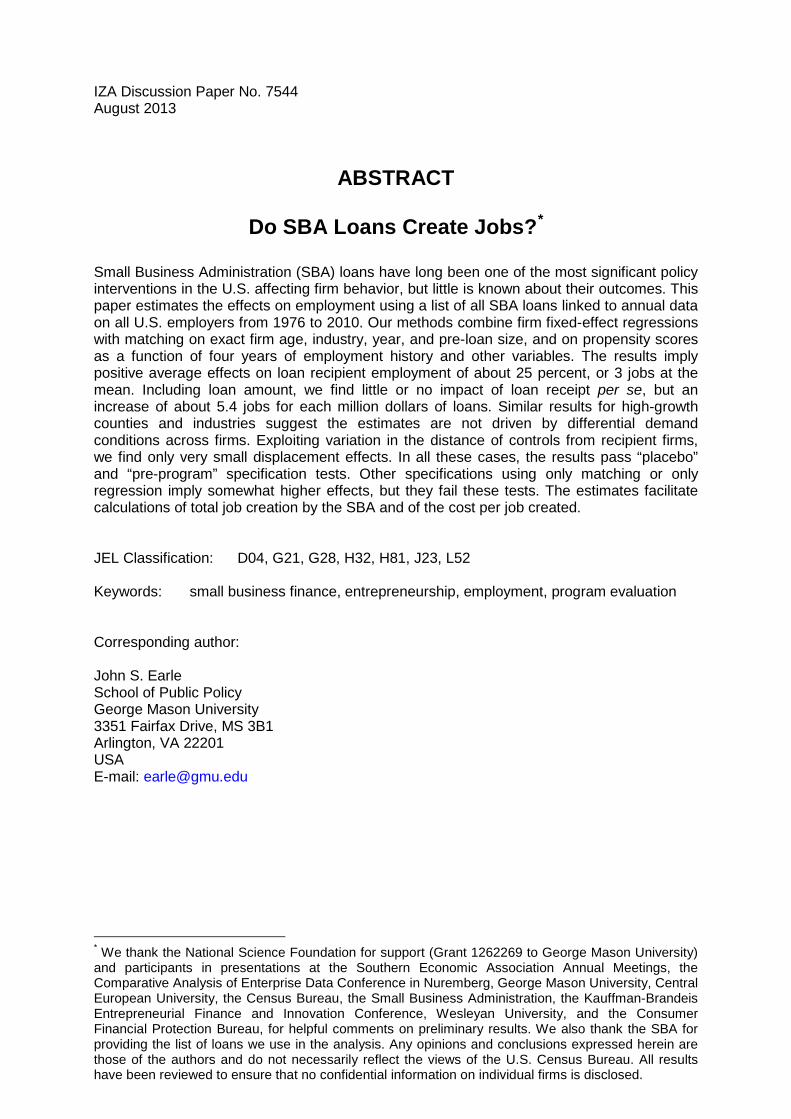
We can also diagnose potential selection bias in these specifications by estimating the

dynamics of the loan effects in event time, and the results are shown in Figures 2 and 3 for these

24

two specifications. Both figures show substantial pre-loan effects of loan receipt with a strong

positive trend. The upward rise continues in the postloan period, but this analysis implies that

the results without matching are likely plagued by too much selection bias to allow reliable

inferences about the impact of these programs.

Thus, we turn to the combined matching with regression estimator, where we use similar

regressions to those just described, but the sample follows the matching procedures described in

the previous section. The results in Table 8 are organized similarly to those in Table 7, with

log(employment) and unlogged employment as dependent variables. The estimates imply

somewhat smaller effects than the previous results: with log(employment) as dependent variable

we estimate an average effect of 24 log points increase in employment associated with receiving

the loan. For unlogged employment, the estimate implies an average treatment effect on the

treated firms of 3.1 additional jobs. Columns (3) and (4) again permit the effect to vary with

Loan Amount, with coefficients rather similar to those we saw in Table 7: slightly smaller in

Column (3) and slightly larger in Column (4). Very different, however, are the estimated

coefficients on the Postloan Dummy in these two specifications, which are much smaller and

statistically insignificantly different from zero, the magnitude declining in the quadratic

specification to the tiny value of 0.20. This implies that the employment gain from loan receipt

is associated only with the amount of the loan, not with selection into the treatment group,

evidence that our matching procedures may be working to reduce selection bias in the

estimates.25

The combined matching-regression estimator passes this “placebo test.”

Figure 4 contains the results from using the combined matching-regression procedure to

estimate the event-time dynamics of the loan effects. The pre-loan period allows us to assess the

25

Estimates from a quartic specification in Loan Amount produced a small negative coefficient on the Postloan

Dummy, which taken literally would imply negative selection into the SBA loan programs.

25

“pre-program test,” and by contrast with the other estimators, here we find only tiny, statistically

insignificant differences between the treated and control firms during this period. In the post-

loan period, we observe big jumps in employment in both the loan year and year following:

about 20 percent total. The jump in the loan year may be explained by anticipatory hiring or

receipt of the loan early in the calendar year. After two years, the growth diminishes, but the

estimates imply the employment effect never falls over the 10-year period we observe. An

interpretation of these results is that the SBA loan, rather than crowding out alternative sources

of finance, may “crowd in” by making it possible for firms to develop a credit history and gain

regular access to formal financial markets.

The combined matching-regression method is our preferred approach because, unlike the

estimators based on only treated firms, or using only matching or only regression methods, the

combined method satisfies the balancing, placebo, and pre-program tests. The tests results

support, but of course cannot definitively prove, the basic identifying assumption that the

combined method has eliminated unobserved differences in demand for loans by firms that are

correlated with differences in their growth potential. If this assumption is invalid, then it might

be the case that the effects we estimate reflect selection bias in which types of firms are loan

recipients. Note that the inclusion of firm fixed effects in the regressions implies that such a

residual selection bias must be time-varying. Furthermore, the dynamics results in Figure 4

imply that there would have to be a demand shock exactly in the loan year and following year.

Any other form of selection bias, such as a more rapid trend growth rate prior to loan receipt,

would have been reflected as such in Figure 4.

26

5.2 Robustness and Displacement

As noted in the previous sub-section, our inclusion of firm fixed effects and our analysis

of dynamics showing no differences in the level or trend of employment between treated and

untreated firms in the pre-treatment period imply that any selection bias must be time-varying,

reflecting for example a positive demand shock received by treated firms – but not by controls –

precisely during the treatment year.26

As discussed in Section 4.3, the identifying assumption for

our estimates to be interpreted as causal is that treatment is independent of a contemporaneous

demand shock. One way of assessing this possibility is to focus on situations where all firms

face a strong increase in demand and thus have good growth possibilities.

For this purpose, we focus on unusually rapid growth environments, which we define two

alternative ways. The first is based on high growth in the same county and year that a treated

firm receives a loan. We define high growth as county-years in the top decile of county-level

employment growth rates over the whole sample; the average employment growth in these cases

is 22.2 percent, and the minimum (i.e., the 90th

percentile) is 10.9 percent – compared with a

county-year average of 0.18 percent. The second approach narrows the definition still farther by

focusing on industry-county-years in the top decile of all industry-county-years in the data; in

this case, the minimum industry-county-year employment growth of the decile is 36.4 percent

and the mean within the top decile is 67.5 percent. We restrict both the treated firms and

controls to come from these unusually high growth situations. If loan receipt is just reflecting a

greater opportunity for growth among treated firms, then the estimate with this high-growth-

26

It is also noteworthy that we found that SBA loan recipients tend to grow for several years prior to the loan, and

we have therefore selected a control group exhibiting similar growth; thus, the distinction between SBA recipients

and non-recipients is not that some “want to grow” and others do not: in our estimates, both groups are growing

prior to the loan at the same rate, but beginning immediately afterwards the recipients grow distinctly faster. The

fact that the matched controls are also growing makes it more likely that they receive conventional loans, without

SBA support, than if we were comparing to the whole population of non-treated firms.

27

context sample should be zero, or at least attenuated compared to the full matched sample

estimates in Table 8. The results shown in Table 9, however, are rather similar to those for the

full data: slightly smaller for the coefficients on Postloan in the county-year definition of high

growth in Panel A, and slightly larger for the industry-county-year definition and for the Loan

Amount specifications. The dynamics of the Postloan coefficient in loan-event time, shown in

Figures 5 and 6, are also qualitatively similar, with only tiny differences in treated and control

firms prior to loan receipt and large sustained jumps immediately afterward. Because these

samples are smaller, the 99 percent confidence intervals are wider, of course. Overall, there is no

evidence from these analyses that differences in demand conditions drive our results.

Another approach to assessing the unconfoundedness assumption is to compare results

with different control groups. If the selection bias into treatment differs across these groups,

then the estimated effects should differ depending on which is used (Imbens and Wooldridge

2009). In our context, we may define alternative control groups geographically, by distance

from the treated firm. Nearby controls (in the same narrow industry and size and age groups) are

more likely to be subject to the same or similar demand shocks as the treated firms, while those

far-away are less so. To implement this procedure, we divide the controls within the kernel

bandwidth according to the distance from treated firm and estimate separately for nearby and

faraway controls. Distance is defined two different ways: in the first, controls are included if

they are up to 10 miles away to constitute the “nearby” group, which is compared to a “faraway”

group more than 50 miles distant from any SBA loan recipient; in the second procedure, we

simply take the nearest four controls for the “nearby” group and the furthest four as “faraway.”

We also have an additional motivation for this geographic analysis. Our methods are

designed to estimate the “average treatment effect on the treated” (ATT), the direct effect on

28

firms receiving loans, and they assume the program has no effect on non-treated firms used as

controls in the analysis.27

Because only a tiny fraction of firms in the U.S. receive SBA-backed

loans, this assumption is plausible. But it is nevertheless possible that even if treated firms grow

as a result of loan receipt that the program creates general equilibrium effects, or spillovers on

other firms. Spillovers may be positive if the loan enables innovation that is somehow copied or

imitated by other firms, or if suppliers or customers benefit together with the loan recipient.

They could also be negative if they are displacement effects that reduce employment at non-

treated firms that compete with the treated in product and labor markets. In either case, the total

job creation – including these indirect effects as well as the direct effect – would differ from the

direct effect we have estimated.

Estimating such general equilibrium effects is intrinsically difficult, and it is largely

ignored in the program evaluation literature (Heckman et al., 1999). Positive spillovers would

imply that our estimates of the direct effect are lower than the total estimate, and therefore we

focus attention here on the possibility of negative displacement effects. If these result from

product market competition, where loan receipt gives the beneficiary an advantage over its

competitors, then we should look for negative effects within industries. If the degree of

competition is related to geographic distance, then we should look for larger negative effects

nearer to treated firms than farther away. In turn, this implies that the estimated ATT should be

larger when the controls are drawn from close by than when they are far away.

Results are shown in Table 10 and dynamics of the estimated effects in Figure 7. In all

cases, we find slightly larger coefficients using nearby controls than we do with faraway

controls. These differences are inconsistent with correlated demand shocks among firms in

27

The program evaluation literature sometimes refers to this as the “stable unit treatment value assumption”

(SUTVA) (Imbens and Wooldridge 2009).

29

closer geographic proximity, but the pattern could result from displacement, however, as nearby

controls grow more slowly as a result of the loan. But the differences are slight, implying only a

small role for displacement – on the order of 0.5 percentage points of the employment effect or

0.1 jobs from the unlogged specification, on average per loan.

A more direct way to compare the nearby and faraway controls, and thus to measure the

displacement effect, is through a “pseudo-outcome test” (Imbens and Wooldridge 2009). The

procedure uses the nearby control group as the treated group, estimating the difference between

them and the faraway controls, defined as above. The results, reported in Table 11, show that the

nearby control group has about two percent fewer jobs (0.26 fewer jobs in the unlogged

specification of Panel B) relative to the faraway control group, though only the coefficient in the

log specification is statistically significant. This again suggests a small displacement effect.

The analysis so far assumes no differences in survival rates between treated firms and

controls, although the SBA frequently refers to business survival as a performance measure, and

access to loans may well affect survival. The direction of the effect is not certain, however,

because while more finance may help a business through hard times, the increased leverage and

possible over-extension may create greater vulnerability. Nor is the measurement of survival

unambiguous, and any disappearance from the database is classified as an exit. Though great

effort has been made to link establishments across time in the LBD, we cannot always

distinguish bankruptcy and other genuine shutdowns from buy-outs or reorganizations that lead

to a change in the identifying code in the LBD. As some of these outcomes represent business

failure, others reflect success, and some level of exit is a normal feature of a dynamic economy,

the analysis of exit is thus also not as clear normatively as our analysis of employment effects.

30

With these qualifications in mind, we are nonetheless interested to ascertain the degree to

which our results might be driven by exit effects. For the final matched sample, exit rates (by

2010, the last year in the LBD) are 45.94 percent for treated firms and 53.62 percent for controls

(kernel weighted, as in the regressions, for greatest comparability). A crude comparison

therefore suggests a higher survival rate associated with treatment, but this does not take into

account the timing of exit or the size of firms exiting. Assuming exit represents job loss, then if

exit is more common among loan recipients, our earlier results are overstated in ignoring the

employment decline associated with exit. On the other hand, if SBA-backed loans raise survival,

our earlier results could be understated. To distinguish these alternatives, we impute a zero value

for employment two years following exit and re-estimate the specifications in Table 8. The

results, shown in Table 12, are slightly larger but qualitatively similar to those without the

imputations, so we conclude that different patterns of exit are unlikely to play an important role

in our results. Further analysis of exit effects, including the characteristics of survivors and

exitors, could be of considerable interest, but we leave it for future research.

6. Conclusion

Our estimates of the effects of the SBA loan programs on employment in this paper are

based on an unusual linking of administrative and census data and an application of econometric

methods originally designed for evaluating job training interventions. We exploit the large size

and completeness of the data to combine matching and regression methods. The first step is to

match exactly on firm age, industry, year, and pre-loan size, and the second is to carry out

kernel-based matching on propensity scores estimated as a function of four years of employment

31

history and other variables. Having constructed the matched sample, we estimate program

effects using firm fixed effect regressions.

The estimation results show positive average effects on loan recipient employment of

about 25 percent or 3 jobs at the mean. Including loan amount, the results imply an increase of

about 5.4 jobs for each million dollars of loans. Examining situations where most small firms

should have excellent growth potential, defined as high growth county-years (average growth of

21.2 percent) or industry-county-years (average growth of 67.5 percent), we find similar effects,

implying that the estimates are not driven by differential demand conditions across firms.

Results are also similar regardless of distance of control from recipient firms, suggesting only a

small role for displacement effects. In all these cases, the results from our preferred specification

combining matching with regression pass a “pre-program” specification test, where controls and

treated firms look similar in the pre-loan period, as well as a “placebo” test, where we find no

effect of program participation per se but an effect increasing with loan size; both of these are

consistent with an important role for finance rather than selection in driving the different

evolution of employment in treated compared to control firms in the post-treatment period.

Because we cannot identify other sources of finance, in particular non-SBA finance received by

the control firms, our estimates may be interpreted as program effects, and possibly as lower

bounds on the effects of the availability of finance more generally. Other specifications, such as

those using only the treated firms or using only matching or only regression methods imply

somewhat higher effects, but they fail the pre-program and placebo tests.

Clearly, these estimates are averages that take no account of a number of dimensions of

heterogeneity. For example, the literature on firm growth, age, and size suggests the interesting

question of whether small versus large versus young firms are more responsive to an easing of

32

credit constraints. Together with industry and regional characteristics, results for these variables

may provide useful information for targeting firms in future loan programs. Another interesting

set of questions concerns the heterogeneity with respect to program characteristics such as

interest rate, term, and SBA program design. A final example concerns the economic

environment, including the state of the business cycle, with its relevance for the role of loans in

macroeconomic stabilization. This paper has ignored all of these dimensions of heterogeneity.

Nevertheless, our estimates of average effects allow rough calculations of the overall job

creation attributable to SBA loans. For this purpose, let us assume the coefficients in Table 7,

which are estimated over the period of 1976-2010, can be applied to the “$30 billion in lending

support to 60,000 small businesses” reported by the SBA for fiscal year 2011. One estimate uses

the specification in column (1) to multiply the Postloan dummy coefficient of 3.083 increase in

employment per loan times the 60,000 small businesses receiving loans to obtain an estimate of

184,980. The second uses column (2) and multiplies 60,000 by 0.708 plus 30 billion dollars

times 5.385 jobs per million dollars for a total of 204,030. The two estimates are rather close,

and although they are significantly less than the claimed half-million or more “jobs created and

retained” by the SBA each year, they are not in an entirely different order of magnitude. On the

other hand, these estimates are for 2011, which saw an unusually large volume of both number

and value of SBA loans; for most other years, the estimated job creation would be lower.

It is important to remember a number of caveats to our estimates. As we have discussed,

the inability to distinguish disbursed from non-disbursed loans and to fully link the SBA data

with the LBD imply measurement error in the treatment variable. We have excluded start-ups,

non-employers, and multi-establishment firms (because of lack of history on which to match and

of identifying the establishment benefitting from the loan). Under plausible assumptions, which

33

we have described, these imply our estimates may be downward biased. On the other hand, the

estimates could also be further refined by permitting heterogeneous effects for different groups,

regions, and time periods, which could lead to lower or higher estimates of overall job creation.

Pursuing these extensions is a high priority for future research.

An additional caveat concerns external validity. In general, estimates of the average-

treatment-effect-on-the-treated can be extrapolated to non-treated sub-populations only under

strong assumptions, but our analysis demonstrates a particular reason for caution. We find that

SBA loan recipients tend to grow for some time before they receive the loan, a pre-program

trend that our matching procedure must address in identifying similar controls. Our analysis of

bias in the covariates suggest the matching procedure has been successful in identifying controls

with similar growth (and other characteristics), and thus that the analysis compares growing

treated with growing control firms, not with the many non-treated small firms that never grow.

Therefore, our results should not be interpreted as implying similar responsiveness to policy

among all small firms, including the many who do not grow and do not want to grow (Hurst and

Pugsley 2011), but they may be relevant for the sub-group of small firms that show growth for a

significant period prior to receiving an SBA loan.

It bears emphasis that our study is not a cost-benefit analysis. It does not estimate the full

benefits of the program, which would include producer surplus of borrowers, lenders, and

workers; possible consumer surplus (if loans help firms to produce at lower cost and result in

lower prices); possible positive spillovers into other sectors; and any external effects of increased

employment for society or the government budget. Our estimates do permit us, however, to

calculate a rough range on the cost per job created by the SBA programs. Assuming an average

guarantee rate of 75 percent, an overall default rate of 18 percent taking place at an average

34

balance of 80 percent with an average recovery rate of 30 percent, and using our estimate of 5.4

jobs per million dollars of loans implies a cost per job of about $14,000.28

Applying a 99 percent

confidence interval (based on the standard error of 0.8) around the point estimate of 5.4 yields a

range of $9,200 to $18,800 cost per job created. This range is far to the left of the usual

estimated cost per job of government programs. Neumark (2013), for instance, reports the cost

from fiscal stimulus under the American Recovery and Reinvestment Act (based on estimates

from Congressional Budget Office 2010) to lie in the range of $158,000 to $407,000, and the

cost per job from a hiring credit under the New Jobs Tax Credit (based on Bartik and Erickcek

2010) at $37,500-$75,000. A full assessment of costs should account for possible distortions,

such as those highlighted by Hurst and Pugsley (2011), and opportunity costs of the funds, but

these figures suggest that compared with the alternatives SBA loan programs may be a relatively

low-cost policy to generate employment.

28

The formula is ($1mln/5.4)*(guarantee rate)*(default rate)* loan balance*(1-recovery rate). The guarantee rate is

from our data, the default and balance rates are from Glennon and Nigro (2005), and the recovery rate is based on de

Andrade and Lucas (2009, Figure 4). The calculation does not consider lender fees to SBA (about $10mln in 2011)

or SBA administrative costs (127mln for both 7(a) and 504 programs, or less than $1000 per job in 2011). The

formula implies a total cost to the SBA of $2.6-2.8mln, not very different from the “fair market value” calculation of

CBO (2012), although significantly higher than the official procedures under the Federal Credit Reform Act, which

would imply still lower cost estimates per job created through the SBA programs.

35

References

de Andrade, Flavio, and Deborah Lucas, “Why Do Guaranteed SBA Loans Cost Borrowers So

Much?” Working Paper, Northwestern University, 2009.

Bartik, Timothy J., and George Erickcek, “The Employment and Fiscal Effects of Michigan’s

MEGA Tax Credit Program.” Upjohn Institute Working Paper No. 10-164. 2010.

Beck, Thorsten, “The Econometrics of Finance and Growth.” Palgrave Handbook of

Econometrics (Terence C. Mills and Kerry Patterson, eds.), Palgrave Macmillan, 2009.

Birch, David L., Job Creation in America: How Our Smallest Companies Put the Most People to

Work. New York: Free Press, 1987.

Clementi, Gian Luca, and Hugo A. Hopenhayn, “A Theory of Financing Constraints and Firm

Dynamics.” Quarterly Journal of Economics, Vol. 121(1), 229-265, 2006.

Congressional Budget Office (CBO), “Estimated Impact of the American Recovery and

Reinvestment Act on Employment and Economic Output from April 2010 through June 2010.”

CBO, 2010.

Craig, Ben R., William E. Jackson III, and James B. Thomson, “The Economic Impact of the

Small Business Administration’s Intervention in the Small Firm Credit Market: A Review of the

Research Literature.” Journal of Small Business Management, Vol. 47(2), 221–231, 2009.

Davis, Steven, John Haltiwanger, and Scott Schuh, Job Creation and Destruction. Cambridge,

Mass: The MIT Press, 1996.

Dilger, Robert Jay, “Small Business: Access to Capital and Job Creation.” Congressional

Research Service Reports to Congress, May 2013.

Glennon, Dennis, and Peter Nigro, “An Analysis of SBA Loan Defaults by Maturity Structure.”

Journal of Financial Services Research, Vol. 28(1/2/3), 77-111, 2005.

Haltiwanger, John, Ron Jarmin, and Javier Miranda, “Who Creates Jobs? Small vs. Large vs.

Young.” Review of Economics and Statistics, Vol. 95(2), 347-361, May 2013.

Heckman, James, and Joseph V. Hotz, “Choosing among Alternative Nonexperimental Methods

for Estimating the Impact of Social Programs: The Case of Manpower Training.” Journal of the

American Statistical Association, Vol. 84(408), 862-74, December 1989.

Heckman, James J., Hidehiko Ichimura, and Petra E. Todd, “Matching as an Econometric

Evaluation Estimator: Evidence from Evaluating a Job Training Programme.” Review of

Economic Studies, Vol. 64(4), 605-654, 1997.

Heckman, James J., Hidehiko Ichimura, and Petra E. Todd, “Matching as an Econometric

Evaluation Estimator.” Review of Economic Studies, Vol. 65(2), 261-294, 1998.

Heckman, James J., Robert J. LaLonde, and Jeffrey A. Smith, “The Economics and

Econometrics of Active Labor Market Programs.” In Handbook of Labor Economics, Vol. 3A.

Edited by Orley Ashenfelter and David Card. Elsevier Science B.V., Amsterdam, 1999.

Hubbard, R. Glenn, “Capital-Market Imperfections and Investment.” Journal of Economic

Literature, Vol XXXVI, 193-225, March 1998.

36

Hurst, Erik, and Benjamin Wild Pugsley, “What Do Small Firms Do?” Brookings Papers on

Economic Activity, 73-118, Fall 2011.

Imbens, Guido W., and Jeffrey M. Wooldridge, “Recent Developments in the Econometrics of

Program Evaluation,” Journal of Economic Literature, Vol. 47(1), 5-86, 2009.

Jarmin, Ronald S., and Javier Miranda, “The Longitudinal Business Database.” CES Working

Paper 02-17, 2002.

Levine, Ross, “Finance and Growth: Theory and Evidence.” In Handbook of Economic Growth,

Philippe Aghion and Steven Durlauf (eds.). Netherlands: Elsevier Science, 2005.

Neumark, David, “Spurring Job Creation in Response to Severe Recessions: Reconsidering

Hiring Credits.” Journal of Policy Analysis and Management, Vol. 32(1), 142-171, 2013.

Neumark, David, Brandon Wall, and Junfu Zhang, “Do Small Businesses Create More Jobs?

New Evidence for the United States from the National Establishment Time Series.” Review of

Economics and Statistics 93(1), 16-29, 2011.

Parker, Jonathan A., “On Measuring the Effects of Fiscal Policy in Recessions.” NBER

Working Paper No. 17240, 2011.

Parker, Jonathan A., Nicholas S. Souleles, David S. Johnson, and Robert McClelland,

“Consumer Spending and the Economic Stimulus Payments of 2008.” NBER Working Paper

No. 16684, 2011.

Ramey, Valerie A., “Identifying Government Spending Shocks: It’s all in the Timing.” Quarterly

Journal of Economics, Vol. 126(1), 1-50, 2011.

Rosenbaum, P., and D. B. Rubin, “Constructing a Control Group Using a Multivariate Matched

Sampling Method that Incorporates the Propensity Score.” The American Statistician, Vol. 39,

pp. 33-38, 1985.

Stiglitz, Joseph, and Andrew Weiss, “Credit Rationing in Markets with Imperfect Information.”

American Economic Review, Vol. 71, 393-410, 1981.

Small Business Administration (SBA), http://www.sba.gov/about-sba-info/11572, 2013a.

SBA, http://www.sba.gov/sites/default/files/files/1-508%20Compliant%20FY%202013%

20CBJ%20FY%202011%20APR%281%29.pdf , 2013b.

SBA, http://www.sba.gov/sites/default/files/files/2-508%20Compliant%20Appendix%

20FY%202012%20CBJ%20FY%202011%20APR%281%29.pdf, 2013c.

SBA, http://www.sba.gov, 2013d.

Whitehouse.gov, “Weekly Address: President Obama Calls for New Steps to Support America’s

Small Businesses,” February 6, 2010.

37

Table 1

Path from Full SBA Loan Dataset to Treated Firms in Final Matched Regression Sample

Number

Total SBA Loans in 1977-2009 1,378,501

Except loans not matched to any business register 763,583

Except loans matched to non-employer business register 604,023

Except firms with first SBA loan before 1977 or a SBA disaster

loan before first SBA 7(a)/504 loan 528,753

Except SBA 7A/504 loans after the first loan 493,116

Except start-ups 337,148

Except multi-establishment firms prior to loan 318,207

Except firms with missing employment in year before loan receipt 269,623

Except firms without matched controls (main sample for analysis) 216,023

38

Table 2

Sample Comparisons among SBA Loan Recipients

Not in Final Sample Final Sample

Not Linked,

Non-Start-Up

Missing

Employment

No Control

Firms Found

Total Number 398,088 48,584 53,600 216,023

Mean Employment 11.87 8.86 16.73 14.80

Mean Loan Amount 339,469 285,527 415,857 400,164

Median Loan Amount 138,789 138,978 250,256 196,329

Percent Sole

Proprietorships

39.09 20.02 13.47 18.74

Percent Partnerships 5.35 4.10 3.33 3.49

Percent Minority 28.00 22.96 13.51 21.29

Percent Female 27.59 27.68 22.25 26.17

Percent Veteran 11.23 10.83 13.79 11.47

Percent By Sector:

Construction 6.39 9.40 5.73 9.19

Manufacturing 5.50 6.22 14.36 7.16

Wholesale Trade 4.70 4.93 6.38 5.39

Retail Trade 12.90 11.08 10.33 11.66

Finance/Insurance/

Real Estate

2.69 2.51 1.37 2.36

Services 33.89 29.98 17.52 31.18

Other/Unknown 33.93 35.88 44.31 33.06 Notes: The variables come from the SBA loan recipient database and generally refer to the year before the loan.

“Not linked” means we were unable to match these firms to any business register. Loan amounts are in constant

2010 US$.

39

Table 3

Descriptive Statistics

All Non-Treated Firms All Treated Firms

Employment Mean 12.54 12.46

Employment Standard Deviation 129.70 26.91

Employment Median 4 6

Age Mean 8.20 6.74

Age Standard Deviation 7.61 6.59

Age Median 6 4

Percent by Sector:

Construction 11.15 10.80

Manufacturing 5.36 12.62

Wholesale Trade 6.21 10.83

Retail Trade 8.22 12.58

Finance/Insurance/Real

Estate

2.55 1.87

Services 55.47 44.93

Other 11.05 6.37 Notes: This excludes multi-establishment firms and establishments that were ever in a multi-establishment firm in

the past. Non-treated firms are included in each year they appear in the LBD, while treated firms are included only

in the treatment year. For treated firms, employment is measured in the year prior to treatment. The variables come

from the LBD.

40

Table 4

Number of Firms and Firm-Year Observations in Regressions with All Matches

Number of

Firms

Pre-Treatment

Firm-Years

Pre-Treatment

Years/Firm

Post-

Treatment

Firm-Years

Post-

Treatment

Years/Firm

Treated 216,023 2,051,524 9.5 1,353,043 6.3

Controls 3,508,245 30,404,010 8.7 15,756,467 4.5 Notes: The year of loan receipt is included with pre-treatment years in this table. Controls are included within a

10% bandwidth around the treated firm’s propensity score.

41

Table 5

Bias Before and After Propensity Score Matching

Variable Mean

All Non-

Treated

All

Treated

Final Treated

Sample

Final Control

Sample

Final %

Bias

% Bias

Reduction

Log Emp t-1 1.307 1.702 1.847 1.879 -2.473 92.050

Log Emp t-1 sq. 3.455 4.374 4.696 4.791 -1.781 89.739

Log Emp t-1 – t-2 0.107 0.229 0.228 0.220 1.198 93.708

Log Emp t-2 – t-3 0.095 0.186 0.198 0.192 0.909 94.176

Log Emp t-3 – t-4 0.082 0.151 0.164 0.162 0.449 96.474

Log Wage 2.151 2.625 2.963 2.985 -1.641 95.297

Age 7.496 7.160 8.030 8.239 -2.928 37.624 Notes: % bias is the standardized difference, which for a given variable, say age, is

( )

∑ [ ∑ ( ) ]

√ ( ) ( )

. The all non-treated group is included in all years they appear in the

LBD. The other three groups are included only in the treatment year.

42

Table 6

Mean Employment in the Unmatched and Matched Samples

Pre-Treatment Post-Treatment

Without Matching:

Treated 11.91 20.90

Non-Treated 15.69

With Matching:

Treated 10.84 20.17

Non-Treated (Controls) 12.44 18.96 Notes: The year of loan receipt is included as a pre-treatment year. The post-treatment years for matched non-treated

firms are the post-treatment years of the treated firms to which the non-treated firms are matched; the treatment year

is undefined for untreated firms without matching, so their mean (15.69) is shown over the entire observation period.

43

Table 7

Estimates from Regressions without Matching

(1) (2) (3) (4)

Dependent variable Log Employment Employment Employment Employment

A. Treated Firms Only

Independent variables:

Postloan Dummy 0.328

(0.002)

3.615

(0.085)

1.325

(0.260)

0.965

(0.107)

Loan Amount 5.463

(0.600)

6.394

(0.195)

Loan Amount2

-0.061

(0.004)

B. Full LBD used as Controls

Postloan Dummy 0.340

(0.088)

3.648

(0.088)

1.197

(0.271)

0.814

(0.096)

Loan Amount 5.526

(0.604)

6.469

(0.197)

Loan Amount2

-0.062

(0.004) Notes: Each column of each panel presents results from a separate regression. The regressions also include year

dummies and firm fixed effects. Standard errors, cluster-adjusted by firm, are in parentheses. Loan amounts are in

2010 $millions.

44

Table 8

Estimates from Combined Matching and Regression using the Final Sample

(1) (2) (3) (4)

Dependent variable Log Employment Employment Employment Employment

Independent variables:

Postloan Dummy 0.242

(0.002)

3.083

(0.101)

0.708

(0.357)

0.203

(0.113)

Loan Amount 5.385

(0.803)

6.613

(0.232)

Loan Amount2

-0.063

(0.004) Notes: Each column presents results from a separate regression. Other regressors include event time dummies

common to treated firms and their matched controls, year dummies, and firm fixed effects (for control firms, there

are separate fixed effects for each treated firm to which they are matched). Loan amount measured in millions of

2010 dollars. Matched sample includes loan recipients and all control firms meeting the exact matching criteria and

with propensity scores lying within a 10% bandwidth. Standard errors, cluster-adjusted by firm, are in parentheses.

Total observations = 49,565,044; treated firm observations = 3,404,567.

45

Table 9

Estimates from Combined Matching and Regression for Samples in Rapidly Growing Counties

and Industries

(1) (2) (3) (4)

Dependent variable Log Employment Employment Employment Employment

Independent variables:

A. Top Decile of County-Year Growth

Postloan Dummy 0.261

(0.012)

2.817

(0.376)

-0.381

(0.413)

-0.811

(0.449)

Loan Amount 7.226

(1.011)

8.601

(1.316)

Loan Amount2 -0.427

(0.169)

B. Top Decile of Industry-County-Year Growth

Postloan Dummy 0.310

(0.019)

4.000

(0.591)

1.446

(0.662)

-0.275

(0.674)

Loan Amount 6.228

(1.202)

13.440

(2.333)

Loan Amount2 -3.356

(1.131) Notes: Results based on the specifications in Table 8, including matching, but with samples restricted to treated

firms and controls in high-growth environments during the loan year. In Panel A, a high-growth environment is

defined as county-years in the top decile of employment growth from the year before loan receipt to the year of

receipt; the mean growth rate is 21.2 percent for these county-years; there are 6,206,928 observations, of which

129,845 are from treated firms, in these regressions. In Panel B, a high-growth environment is defined as industry-

county-years in the top decile of employment growth from the year before loan receipt to the year of receipt; the

mean growth rate is 67.5 percent for these industry-county-years; there are 2,207,589 observations, of which 59,442

are from treated firms, in these regressions (industry is defined at the 2-digit level). As in Table 8, all regressions

also include event time dummies common to both treated firms and their matched controls, year dummies, and firm

fixed effects (for control firms, there are separate fixed effects for each treated firm to which they are matched), but

geography is not used for exact matching among treated and control firms in these samples. Loan amounts are in

millions of 2010 dollars. Standard errors, cluster-adjusted by firm, are in parentheses.

46

Table 10

Regressions with Control Groups Defined by Geographic Distance from Matched Treated Firms

Control Groups <10 miles >50 miles Nearest 4 Furthest 4

Log Employment

1. Postloan Dummy 0.209

(0.007)

0.204

(0.007)

0.203

(0.004)

0.194

(0.004)

Unlogged Employment

2. Postloan Dummy 1.663

(0.128)

1.501

(0.130)

2.277

(0.134)

2.150

(0.146)

3. Postloan Dummy 0.529

(0.134)

0.364

(0.135)

0.444

(0.166)

0.320

(0.175)

Loan Amount 3.524

(0.354)

3.470

(0.352)

4.540

(0.221)

4.532

(0.221)

4. Postloan Dummy 0.187

(0.131)

0.022

(0.132)

-0.001

(0.182)

-0.123

(0.190)

Loan Amount 5.119

(0.484)

5.003

(0.475)

6.143

(0.320)

6.131

(0.320)

Loan Amount2

-0.543

(0.124)

-0.521

(0.121)

-0.405

(0.051)

-0.404

(0.052)

Total Obs. 1,419,964 2,617,849 4,961,474 4,955,124

Treated Firm Obs. 400,854 400,854 1,079,342 1,079,342 Notes: Results based on the specifications in Table 8 (numbered 1-4, as in that table, but for convenience here

arrayed with axes rotated), including matching, but with samples of controls restricted based on their distance

from the matched treated firm. The first control group contains controls located no more than 10 miles away.

The second control group contains those more than 50 miles away from any SBA loan recipient in the treated

firm’s year of loan receipt. The third and fourth control groups are the nearest and furthest four firms from the

treated firms to which they are matched. Only treated firms that have controls in both control groups are

included in the regressions. The regressions also include event time dummies common to both treated firms and

their matched controls, year dummies, and firm fixed effects (for control firms, there are separate fixed effects

for each treated firm to which they are matched). Standard errors, cluster-adjusted by firm, are in parentheses.

Loan amounts are in millions of 2010 $.

47

Table 11

Evidence on Displacement: Pseudo-Outcome Tests with Nearby Controls Acting as Treated

Relative to Far-Away Controls

Log Employment Unlogged Employment

A. Closest 4 Relative to Furthest 4

Postloan Dummy -0.009

(0.003)

-0.079

(0.096)

B. < 10 Miles Relative to > 50 Miles Away

Postloan Dummy -0.019

(0.006)

-0.264

(0.141) Notes: The regressions also include event time dummies common to both treated firms and their matched controls,

year dummies, and firm fixed effects (for control firms, there are separate fixed effects for each treated firm to

which they are matched). Standard errors, cluster-adjusted by firm, are in parentheses. In Panel A, the pseudo-

treatment group is the nearest four non-treated firms to the matched treated firm. The control group is the furthest

four firms from the matched treated firm. Only firms whose matched treated firm appears in the regressions with the

nearest four non-treated firms and furthest four treated firms are included here; there are 7,757,914 observations of

which 3,882,132 are pseudo-treated. In Panel B, the pseudo-treatment group is non-treated firms located no more

than 10 miles away from the matched treated firm. The control group is firms more than 50 miles away from any

SBA loan recipient in the treated firm’s year of loan receipt. Only firms whose matched treated firm appears in the

regressions with non-treated firms no more than 10 miles away and those more than 50 miles away are included

here.

Table 12

Unlogged Employment Regressions with Matched Sample, Imputing Zero Employment in First

Two Years After Exit

(1) (2) (3)

Postloan Dummy 3.305

(0.082)

1.716

(0.349)

1.220

(0.092)

Postloan Dummy*Loan

Amount

3.701

(0.811)

4.920

(0.204)

Postloan Dummy*Loan

Amount2

-0.045

(0.002)

Total Obs. 55,883,482

Treated Firm Obs. 3,704,108 Notes: The regressions also include event time dummies common to both treated firms and their matched controls,

year dummies, and firm fixed effects (for control firms, there are separate fixed effects for each treated firm to

which they are matched). Standard errors are cluster-adjusted by firm. The loan amount is in $millions. Zero

employment is imputed in the first two years after exit. The percent of firms exiting prior to 2010 is 45.9 percent for

treated firms and 53.6 percent for their matched controls.

48

Table A1

Passes Used for Matching SBA Loan Data to Census Bureau Employer and Non-Employer

Business Registers

Pass 1 Pass 2 Pass 3 Pass 4 Pass 5

Exact match on 5-digit zip code X X X

Exact match on standardized street address X

Exact match on standardized business name X X

Exact match on 3-digit zip code X

Standardized street soundex (phonetic algorithm) X

Street address allowing for fuzziness (70%

sensitivity in SAS DQMATCH)

X

Business name allowing for fuzziness (70%

sensitivity in SAS DQMATCH)

X X X

Place (city) soundex X

Street name allowing for fuzziness (70%

sensitivity in SAS DQMATCH)

X

Street number allowing for fuzziness (70%

sensitivity in SAS DQMATCH)

X

49

Figure 1. Mean Firm Employment by Year Before/After Loan

9

11

13

15

17

19

21

23

25

-7 -6 -5 -4 -3 -2 -1 0 1 2 3 4 5 6 7 8 9 10

Years Before/After Loan

treated firms matched non-treated firms

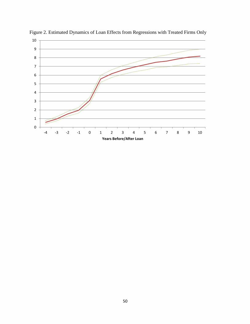
50

Figure 2. Estimated Dynamics of Loan Effects from Regressions with Treated Firms Only

0

1

2

3

4

5

6

7

8

9

10

-4 -3 -2 -1 0 1 2 3 4 5 6 7 8 9 10

Years Before/After Loan

51

Figure 3. Estimated Dynamics of Loan Effects from Regressions with All LBD (no matching)

-1

0

1

2

3

4

5

6

-4 -3 -2 -1 0 1 2 3 4 5 6 7 8 9 10

Years Before/After Loan

52

Figure 4. Estimated Dynamics of Loan Effects from Regressions with Final Matched Sample

-1

0

1

2

3

4

5

6

-4 -3 -2 -1 0 1 2 3 4 5 6 7 8 9 10

Years Before/After Loan

53

Figure 5. Estimated Dynamics of Loan Effects from Regressions with Matched Sample

Restricted to County-Years in the Top Decile of Employment Growth Rates

-2

-1

0

1

2

3

4

5

6

-4 -3 -2 -1 0 1 2 3 4 5 6 7 8 9 10

Years Before/After Loan

54

Figure 6. Estimated Dynamics of Loan Effects from Regressions with Matched Sample

Restricted to Industry-County-Years in the Top Decile of Employment Growth Rates

-2

0

2

4

6

8

10

-4 -3 -2 -1 0 1 2 3 4 5 6 7 8 9 10

Years Before/After Loan

55

Figure 7. Estimated Dynamics of Loan Effects from Regressions with Matched Sample

Restricted by Treated-Control Distance

-1

-0.5

0

0.5

1

1.5

2

2.5

3

-4 -3 -2 -1 0 1 2 3 4 5 6 7 8 9 10

Years Before/After Loan

<=10 Miles >50 miles Nearest 4 Furthest 4