1

Do Preferential Trade Policies (Actually) Increase Exports? A comparison between EU and US trade policies

Maria Cipollina

University of Molise, via F. de Sanctis, 86100 Campobasso, Italy. E-mail: cipollina@unimol.it.

David Laborde

International Food Policy Research Institute

Luca Salvatici

Università degli Studi Roma Tre, Via Silvio D’amico 77 – 00145 Roma, Italy. E-mail: lsalvatici@uniroma3.it PRELIMINARY DRAFT NOT TO BE QUOTED

Acknowledgements This work was supported by the “New Issues in Agricultural, Food and Bio-energy Trade (AGFOODTRADE)” (Small and Medium-scale Focused Research Project, Grant Agreement no. 212036) research project funded by the European Commission, and the “European Union policies, economic and trade integration processes and WTO negotiations” research project funded by the Italian Ministry of Education, University and Research (Scientific Research Programs of National Relevance 2007). The views expressed in this paper are the sole responsibility of the authors and do not necessarily reflect those of the European Commission.

2

Do Preferential Trade Policies (Actually) Increase Exports? A comparison between EU and US trade policies

Trade preferences for developing countries have been used by the European Union (EU) and the United States (US) since the early 1960s. Most developing countries (DCs) can export to EU and US with preferential market access under different preferential schemes. Based on cross-section trade data for 2004 and an explicit measure of the intensity of the preference margins at the 8-digit tariff line level, this work estimates and compares the impact on trade of EU and US preference schemes using a theoretical grounded gravity model framework. We use a continuous variable to measure the preference margin adopting a definition that takes into account the duties paid by each exporting country to the EU market. Our results show that trade elasticity estimates are very sensitive to the preference margin definition adopted. From a policy perspective, our results show that preferential schemes have a significant impact on trade in terms of both margins, and such effect seems to be stronger in the case of EU preferences, although with significant differences across products. JEL codes: F13, Q17, F14

In recent years, developed countries, such as EU and US, have increased their use of preferential

regimes in order to promote the economic development as well as the integration of poorest

countries in the world trading system (Bureau et al., 2006). This work provides a comparison of the

impact on trade of European Union (EU) and United States (US) preferences to developing

countries (DCs). To examine this relationship empirically, we use a gravity equation approach in

order to single out the contribution of preferential policies to the deviation from the ‘normal’ trade

levels (Anderson and van Wincoop, 2003) and derive a theoretical grounded gravity equation

including different goods.

This paper is part of the research effort that attempts to assess the various determinants of

bilateral trade at sectoral level using highly disaggregated data (Baldwin et al., 2005; Cardamone,

2009; Disdier et al., 2008; Emlinger et al., 2008). Since trade policies are defined and implemented

at a very detailed level, it is crucial to use disaggregated data and this is one of the strength of the

present analysis since we use data at the 8-digit tariff line level distinguishing preferential and MFN

trade flows. That is, we make use of all the available information about the preference utilization

even if we data do not allow to pin down each trade flow to a specific preferential scheme.1

The use of highly disaggregated data raises two types of problems: (i) the elevated percentage of

‘zero trade flows’; (ii ) the impossibility for some variables to get information at the level of detail at

which tariff lines are specified. As far as the latter problem is concerned, in order to control for the

unobservable country and product heterogeneity we introduce product- and country-specific fixed

effects.

The presence of zero values creates obvious problems in the log-linear form of the gravity

1 In point of fact, the information about the utilization rate of different schemes is available in the case of the United States but not for the European Union.

3

equation. There has been a long debate concerning what is the best econometric approach in order

to avoid the bias that would be implied by the drop of the observations with zero flows. Several

authors consider the Heckman two-step estimator as the best procedure (Linders and de Groot,

2006; Helpman, Melitz and Rubistein, 2008; Martin and Pham, 2008), others argue that gravity type

models should be estimated in multiplicative form, and recommend maximum likelihood estimation

techniques based on the Poisson specification of the model (Siliverstovs and Schumacher, 2007;

Santos-Silva and Tenreyro, 2003, 2006).

Because of the presence of heteroskedasticity, estimates of the log-linear form of the gravity

equation are biased and inconsistent, and this may lead to prefer the Poisson specification of the

trade gravity model. On the other hand, the standard Poisson model is vulnerable for problems of

overdispersion and excess number of zero flows. To overcome the heteroskedasticity (in the case of

the log-normality assumption) and overdispersion (in the case of the standard Poisson specification)

problems, in this paper we make use of the Zero-Inflated Poisson (ZIP) model as in Burger et al.

(2009).

In order to provide an accurate assessment of trade preference impact we compute an explicit

measure of the preferential margins at the most detailed level. Computing the intensity of the

preference margin associated with different trade flows is a significant departure from most of the

literature estimating the impact of preferential agreements through a dummy variable for

preferential policies. Such a dummy do not catch the variability of margins across countries and

products, and it is likely to lead to an overestimation of the impact of the preferential scheme and

cannot provide an accurate assessment of policies that (by definition) often discriminate among

products.

In the most recent but rapidly growing literature using explicit an explicit measure of the margin

several definitions have been used (De Benedictis and Salvatici, 2011). We compute the preference

margins in relative rather than absolute terms, as the ratio between the trade weighted average duty

and the AVE of the applied rates faced by each exporter (Cipollina and Salvatici, 2011).

With respect to the margin definition used in Cipollina and Salvatici (2011), we introduce a

major change in terms of the computation of the ‘reference tariff’, that is the duty paid by the

countries competing with the one benefitting from the preference. In order to avoid potential

overestimation, we need to emphasize the competitive advantage with respect to other

exporters/competitors taking into account the ‘multilateral nature’ of preferential policies. The

intensity of the preferential treatment depends both on the highest paid rate and on the share of

exporters paying that rate. The basic intuition underlying ‘multilateral trade resistance’ in gravity

models suggests that trade is influenced by the trade policies towards all the partners, this means

4

that bilateral trade depends on the whole structure of applied tariffs preferences as well as the

country-pair specific margins. This implies using applied bilateral duties rather than multilateral

(Most Favoured Nation, MFN) ones. Moreover, since we need a single reference tariff for each

product, the exporter-specific duties need to be averaged across exporters. We compare the

estimates obtained using this definition with those resulting from a more ‘traditional’ choice as a

reference, such as the MFN applied duty.2

We estimate cross-sectional models using data on imports at 8-digit level to EU (25 countries)

and US for the year 2004. The structure of the dataset is conditioned by the absence of time series

data on tariffs. It should be noted, though, that the theoretically grounded gravity equation proposed

by Anderson and van Wincoop (2003) under the assumption that all bilateral trade costs are

symmetric and never vary only works with cross section data (Baldwin and Taglioni, 2006). We run

separate regressions for several commodity groups defined according to the Harmonised System

(HS) sections (Table 1). Most of the trade preferences that the EU and US have for developing

countries cover much more than trade issues, such as aid and political cooperation, but in this paper

we will focus strictly on the provisions that are directly trade-related, and particularly on the

differences between the systems. Table 2 shows all preferential schemes included in our dataset

which refers to year 2004.

I. TRADE EFFECTS OF EU AND US PREFERENTIAL POLICIES

One might expect – given the number of preferential schemes implemented over the past forty

years – that the answer to the question posed in this paper’s title is rather accurate. Even if the

expectation of the positive impact of preferences on trade is by far and large confirmed,

international trade economists can actually claim little firm empirical support for reliable

quantitative estimates of the average effect of trade preferences on bilateral trade (all else constant).

It is not an easy task to summarize the results of the large literature assessing the impact of

preferences on trade. Over the past decade, the gravity equation has emerged as the empirical

workhorse in international trade to study the ex post effects of trade preferences on bilateral

merchandise trade flows. Studies report very different estimates, due to the fact that they differ

greatly in data sets, sample sizes, independent variables used in the analysis and estimation

methods. Regarding the estimated coefficients of the impact of preferences, comprehensive surveys

of the estimated PTAs impact are provided by Nielsen (2003) and Cardamone (2007) and, more

recently, Cipollina and Pietrovito (2011).

2 Using the applied rather than bound tariff we avoid the risk of including some ‘water’ (i.e. the binding overhang) into the preference margin.

5

Most studies typically assume a dummy variable to represent the preferential treatment effect

and use aggregate trade data. As far as the EU is concerned, these studies report positive

coefficients ranging between 4% and around 400%, but some specification even find significant

negative coefficients between 3% and more than 50% (Caporale et al., 2009; Peridy, 2005; Ruiz

and Villarubia, 2007; Nilsson, 2002; Martìnez-Zarzoso et al., 2009). In the US case, positive

coefficients range between 6% and around 700%, whereas negative impacts go from 10% to 90%

(Mayer and Zignano, 2005; Koo et al., 2006; Hilbun et al., 2006).

Some studies attempt to pin down the specific impact of different schemes. Lederman and

Özden (2004) estimate that the impact of US preferences ranges between 3% and 33% for the CBI,

while the estimated effects of GSP and AGOA are doubled. Other estimates provide more

conservative, though still positive, results: Nouve (2005), for instance, find that the GSP

beneficiaries increase their export to the US market by 17%, whereas the impact of AGOA is

around 20%. However, it should be mentioned that several studies focusing on the impacts of

AGOA using sectoral analyses obtain an inconclusive evidence (Mattoo, Roy and Subramanian,

2002; Nouve and Staatz, 2003; Shappouri and Trueblood, 2003; Olarreaga and Özden, 2005).

This is not the first paper in empirical international trade to call attention to the importance of

the actual preferential margin(s) and the need to work on highly disaggregated data as in the case of

Cardamone (2009), Emlinger et al. (2008), and Cipollina and Salvatici (2010) for the EU; and

Gaulièr et al. (2004), Jayasinghe and Sarker (2004), and Siliverstovs and Schumacher (2007) for the

US. Several studies find that the EU schemes do provide a significant boost to LDCs exports

(Aiello and Cardamone, 2009; Aiello and Demaria, 2009; Demaria, 2009), and to exports from

Mediterranean countries (Nilsson and Matsson, 2009) as well as from ACP countries (Francois et

al., 2006; Manchin, 2006) though some specifications report highly negative coefficients. In terms

of different schemes, there is some evidence that EBA3 has not been effective in increasing LDCs

exports to the EU (Pishbahar and Huchet-Bourdon, 2008; Gradeva and Martinez-Zarzoso, 2009).

Even if several studies analyze either the effects of EU or US trade preference schemes, only a

few aim to compare them. Bourdet and Nilsson (1997) analyze the impact of EU and US GSP

schemes over the 1976-1992 period and find that the volume of exports that could be attributed to

the EU GSP scheme was significantly larger (in the range of 40%) than the equivalent volume

attributed to the US scheme. Haveman and Schatz (2003) estimate that EU preference programs

have increased exports from LDCs by about 45 per cent, as compared to 10 per cent in case of the

US. This difference in trade generating effect between the EU and US schemes, around 35 per cent,

3 As a matter of fact, the EBA program implemented in 2001 has led to very minor changes in terms of applied protection faced by LDCs for which the previous GSP program was already close to a duty-free regime.

6

is in line with the results obtained in the study by Nilsson (2007). Finally, the literature on the

effects of preference erosion (e.g., Francois et al., 2006) commonly find relatively greater negative

effects of EU trade liberalization on preferences dependent developing countries’ exports compared

to other preference donors, thereby confirming the relative importance of EU preferences.

II. METHODOLOGY

Our set-up is similar to in Lai and Trefler (2002) and Lai and Zhu (2004). Consumers have Cobb-

Douglas preferences over sectors and CES preferences over goods within each sector. With Cobb-

Douglas preferences we can look at one sector at a time: fix the sector and suppress the sectors

index. Let k index goods within each sector. Let j and i index user countries and producer countries,

respectively.

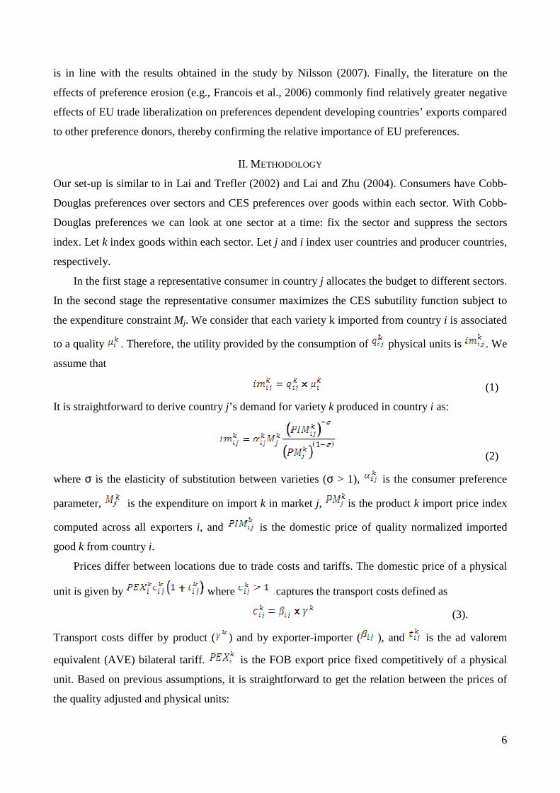
In the first stage a representative consumer in country j allocates the budget to different sectors.

In the second stage the representative consumer maximizes the CES subutility function subject to

the expenditure constraint Mj. We consider that each variety k imported from country i is associated

to a quality . Therefore, the utility provided by the consumption of physical units is . We

assume that

(1)

It is straightforward to derive country j’s demand for variety k produced in country i as:

(2)

where σ is the elasticity of substitution between varieties (σ > 1), is the consumer preference

parameter, is the expenditure on import k in market j, is the product k import price index

computed across all exporters i, and is the domestic price of quality normalized imported

good k from country i.

Prices differ between locations due to trade costs and tariffs. The domestic price of a physical

unit is given by where captures the transport costs defined as

(3).

Transport costs differ by product () and by exporter-importer ( ), and is the ad valorem

equivalent (AVE) bilateral tariff. is the FOB export price fixed competitively of a physical

unit. Based on previous assumptions, it is straightforward to get the relation between the prices of

the quality adjusted and physical units:

7

(4).

We assume that to produce a quality , exporters face a marginal cost , where is the cost

elasticity to quality. Therefore the unit value of exports is given by

(5).

The parameters are chosen so that import quantities are scaled in order to make all the CIF

prices (i.e., including transport costs) equal to 1. Accordingly, the price index can be written as

(6)

then, is a weighted average tariff applied on product k by country j, where the weights are

consistent with the price of the (assumed) CES import demand function4.

Given our focus on exporter-specific preferences, in a cross section analysis we cannot identify

the parameters. So we impose symmetric preferences:

(7).

We are interested in the import share bilateral imports evaluated at domestic prices ( ):

(8).

Using the previous equations and taking the log we get:

(9).

The previous expression is the gravity equation we are going to estimate:

- is the consumer preference parameter for the good k;

- is the market share of exporter i.

- denotes the exporter’s supply price impact as

well as the quality effect’s impact on demand for commodity k: notice that

such a coefficient can be either positive or negative;

- trade cost component;

- is the power of applied tariff; 4 In our approach we assume elasticitiy values of 1.1, 2 and 4.

8

- is the overall price of imports and it is common for all exporters.

The preferential margins ( are given by:

. (10).

The critical issue is the measurement of . The preference margin based on the applied MFN

duty leads to an obvious overestimation of the competitive advantages enjoyed by exporting

countries, since bilateral trade depends on the whole structure of the tariff preferences as well as the

country-pair specific margins. This is very much in line with the basic intuition underlying

‘multilateral trade resistance’ in gravity models, since trade is influenced by the trade policies vis à

vis all the partners in the same way it is influence by relative rather than absolute transport cost.

Accordingly, not only the applied tariff but also the reference tariff we use to compute the margin

enjoyed by exporter i on product k is exporter-specific and computed as a (CES) trade-weighted

average of the duties paid for the given product by each exporter (equation (6)).5

Econometric approach

Working at a highly disaggregated level implies the presence of many zero trade flows that

create obvious problems in the log-linear form of the gravitational equation. All countries do not

produce all available goods, nor do they all have an effective demand for all available goods.

Accordingly, we distinguish between two different kinds of zero-valued trade flows: products that

are never traded and products that are not traded, but could be (potentially, at least) traded. Hence, a

distinction can be made between flows with exactly zero probability of positive trade, flows with a

non-zero trade probability who still happen to be zero, and positive flows. Since preferential

policies cannot possibly influence the first group, in our analysis we only keep exporters that have

at least one export flow at the world level at the HS6 level for the product concerned during the

period 2001-2004, assuming that excluded commodities are not produced. In the same vein, we

exclude products that are not imported at all in the EU and the US. This avoids the inclusion of

irrelevant information that may bias the estimate, and greatly reduces the dimension of the dataset.

The reduced database still includes a large share (80%) of zero flows. These zeros may be the

result of rounding errors: for instance, products for which bilateral trade does not reach a minimum

value, the value of trade is registered as zero. If these rounded-down observations were partially

compensated by rounded-up ones, the overall effect of these errors would be relatively minor.

5 Our reference tariff turns out to be a weighted average of duties paid by actual exporters. This is a shortcoming of the CES functional form that does not take into account the potential competition coming from exporters facing prohibitive tariffs. In this respect our preference margins may be understated and this would lead to an overestimation of the preference impact.

9

However, the rounding down is more likely to occur for small or distant countries and, therefore,

the probability of rounding down will depend on the value of the covariates, leading to the

inconsistency of the estimators. The zeros can also be missing observations which are wrongly

recorded as zero. This problem is more likely to occur when small countries are considered and,

again, measurement error will depend on the covariates. As a consequence, the most common

strategies to circumvent the ‘zero problem’ in the analysis of trade flows – i.e., to omit all zero-

valued trade flows or arbitrarily add a small positive number to all flows in order to ensure that the

logarithm is well-defined – leads to inconsistency.

When the dependent variable is zero for a substantial part of the sample but positive for the rest

of the sample, the econometric theory suggests the use of Tobit models. As is typical in the

literature, many gravity works perform Tobit estimates by constructing a new dependent variable y

= ln(1+Mij). However, this procedure relies on rather restrictive assumptions that are not likely to

hold since the censoring at zero is not a ‘simple’ consequence of the fact that trade cannot be

negative. Zero flows, as a matter of fact, do not reflect unobservable trade values but they are the

result of economic decision making based on the potential profitability of engaging in bilateral trade

at all.

The Heckman two-step procedure transforms a selection bias problem into an omitted variable

problem which can be solved by including an additional variable, the inverse Mills ratio (λ),

between the regressors. However, the Heckman procedure still implements a log-normal model

based on the questionable assumption that the error terms all have the same variance for all pairs of

origins and destinations (homoskedasticity). Especially when there are a large number of cases in

which the observed and expected flows are small, small absolute differences before performing a

logarithmic transformation of the dependent and independent variables may lead to large

differences in the log-normal estimation of the model: in the presence of such heteroskedasticity,

not only the efficiency but also the consistency of the estimators is at stake (Santos Silva and

Tenreyro, 2006). Accordingly, we tested for heteroskedasticity in the first-stage probit, using a two-

degrees-of-freedom RESET test as suggested by Santos-Silva and Tenreryo (2009), and we could

not accept the null hypothesis of homoskedasticity6.

Even if the presence of heteroskedasticity in trade data seems to preclude the estimation of any

model that purports to identify the effects of the covariate, a way to overcome problems

heteroskedasticity and overdispersion is to use the Zero-Inflated Poisson (ZIP) model, recently

suggested by Burger et al. (2009). The ZIP estimator does not rely on stringent normality

6This also rules out the possibility to implement the variant of the two stage procedure proposed by Helpman, Melitz and Rubinstein (2008) to correct for firm-level heterogeneity.

10

assumptions, nor does it require an exclusion restriction or instrument for the second stage of the

equation. With respect to the standard Poisson techniques the ZIP estimator provides a way of

modeling the excess zeros in addition to allowing for overdispersion (Lambert 1992; Greene 1994).

In particular, the estimation process of the ZIP model consists of two possible data generation steps:

the first contains a logit (or probit) regression of the probability that there is no bilateral trade at all;

the second contains a Poisson regression of the probability of each count for the group that has a

non-zero probability or interaction intensity other than zero.

Then, for each observation step 1 is chosen with probability ρijk and step 2 with probability (1-

ρijk). Step 1 generates only zero counts, whereas step 2, Φ(mijk│Xijk), where Xijk is the set of

observed variables in equation (9), generates counts from a Poisson model. The probability of

{ Mijk=mijk│Xijk } is

>−

Φ′−

=−

Φ′−+′

==

0,,)/11(

,|((1{

0,,)/11(

,|0((1{(

),|(

ijk mif )kjT k

ijtkiPEX k

ijijkm)}ijkz

ijk mif )kjT k

ijtkiPEX k

ij)}ijkz)ijkz

ijkz ijkXijkmijkMPε

γβγρ

εγβγργρ

(11).

When the probability ρijk depends on the characteristics of observation ijk , ρijk is written as a

function of γijkz′ , where ijkz′ is the vector of zero-inflated covariates and γ is the vector of zero-

inflated coefficients to be estimated. The probit function that relates the product γijkz′ , which is a

scalar, to the probability ρijk is called the zero-inflated link function.

Then, we estimate the following specification:

(12)

with v as standard error. The preference factor variable (1+prefijk) is associated with the dummy

PRE which is equal to 1 in the case of preferential trade flows and the dummy EU which is equal to

1 if the importer is the EU. In the estimation the trade cost components are proxied by fixed effects

defined for importer, exporter and product, whereas the exporter’s supply price impact, as well as

the quality effect’s impact, is proxied by the unit value by exporter.

III. DATA

All data – i.e., tariffs and trade – refer to 2004. EU trade flows are from the Eurostat database

Comext7, data are Cost-Insurance-Freight (CIF) values. While US trade flows are from the United

States International Trade Commission.

7 The Comext database (http://fd.comext.eurostat.cec.eu.int/xtweb/) contains detailed foreign trade data distinguished by tariff regimes as reported by the EU member states.

11

We consider 234 exporters of 10,174 products at the 8-digit level of EU Combined

Nomenclature classification to the EU (25 countries) and 11,867 products for the US case. The ad

valorem equivalent were computed using the Tarif intégré de la Communauté Européenne (TARIC)

and the US Harmonized Tariff Schedule. We apply a similar methodology to the one applied to

build the MAcMapHS6 version 2 database (Boumelassa, Laborde and Mitaritonna, 2009). In

particular, to convert specific tariffs we use the 8 digit trade flows to compute 8 digit unit values

relying on the same system of filter to avoid outliners. Most DCs and products may be eligible for

several preferential regimes. Since data do not allow to distinguish the specific scheme under which

import take place, we assume that the lowest available duty is the one actually used. For the

treatment of the TRQs we follow Raimondi et al. (2010), thus if imports are no greater than the

quota, the tariff equivalent is the in-quota tariff; alternatively it is the weighted average of the two

tariffs.

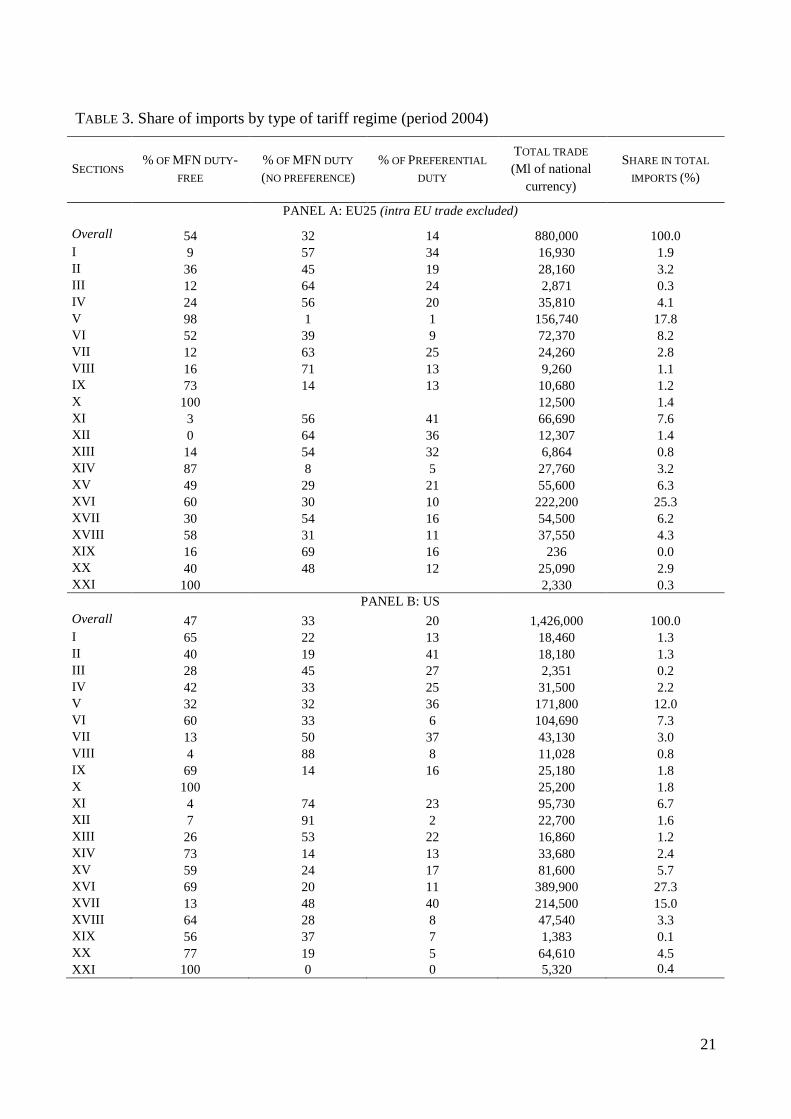
Table 3 shows the percentage of imports associated with positive trade, subject to MFN or

preferential duties (column 4): in the case of MFN imports, we distinguish between duty free

(column 2) and positive tariffs (column 3). To give an idea of the relevance of each section in total

trade, we provide the value of imports (column 5) and their respective shares (column 6). Panel A

reports information from the EU25 dataset, whereas Panel B reports information from the US

dataset.

Something more than 50% of total EU imports enter duty-free under MFN arrangements, the

residual is divided in one third as preferential imports and the remaining as imports paying positive

MFN duties. Looking at Panel B for US, it emerges that around half of products enter under an

MFN duty-free regime, a share of 20% benefit from positive preference margins and around 30%

are MFN duty- imports.

At the section level, both EU and US imports products of section X (paper and paperboard and

articles thereof) and XXI (works of art) under an MFN duty-free regime, while for the other

sections the structure of trade differs considerably. The EU imports a large percentage of products

of sections V (mineral products), IX (wood and articles of wood) and XIV (natural and precious

metals) with a duty-free MFN access, and more than half of products of the remaining sections

without any preferences. On the other side the US imports a large percentage of products of sections

I (live animals and animal products), VI (chemicals), XIV (natural and precious metals), XV (base

metals), XVI (machineries), XVIII (cinematographic and musical instruments), XIX (arms and

ammunition) and XX (other manufactured articles) under a MFN duty-free regime, and most

12

imports other sections take place under a preferential arrangement8.

The Table 4 presents the bilateral applied and MFN tariffs as well as the ‘CES tariffs’ computed

assuming different elasticities (1.1,9 2 and 4). Overall, the EU market appears to be more protected

than the US one. The most protected EU sectors are the agricultural ones (IV, II, III), while this is

not the case for the US where the bilateral applied tariffs are very low for the most sectors, and

higher protection emerges only for raw hides and footwear (VIII, XII). Comparing the MFN tariff

with the CES applied tariffs, the former is always much higher and this leads to inflated preference

margins.

IV. RESULTS

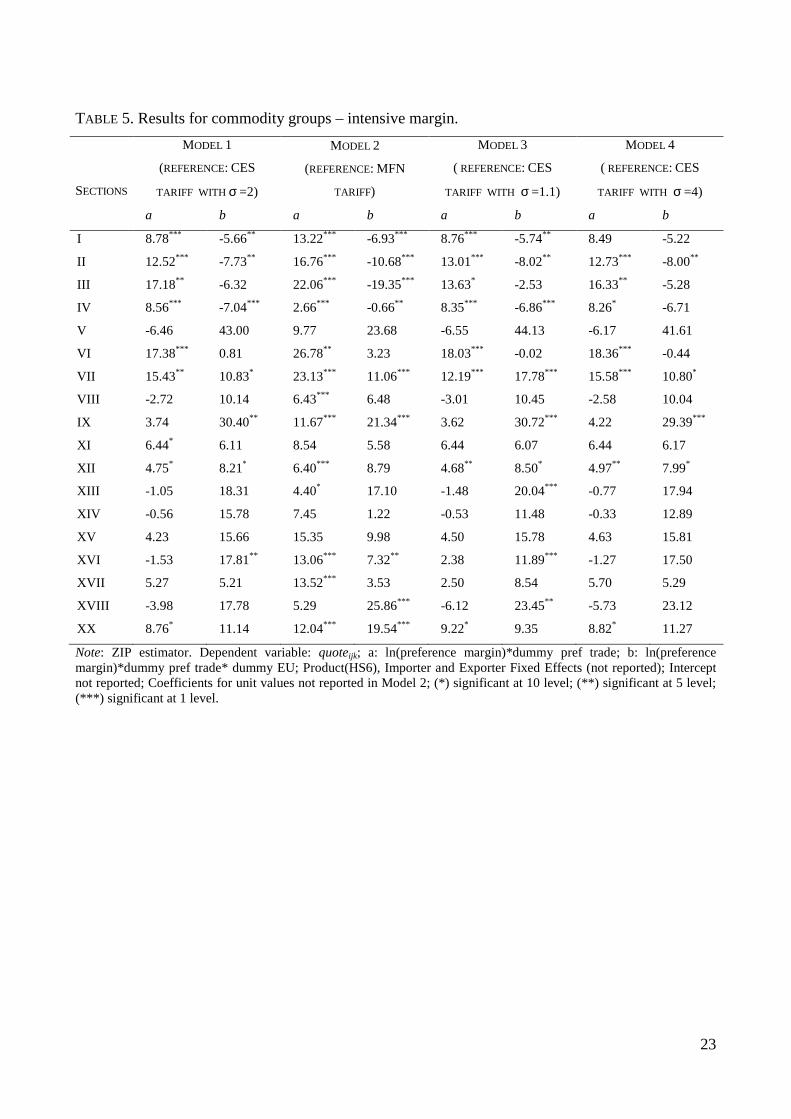
Tables 5 report estimates regarding the preferences by commodity groups. Using different

preference margins the econometric results quantify the extent to which trade preferences have

increased the volume of trade. The Table reports the results for four models: Model 1 is based on the

definition of preference margin using as reference tariff (i.e., the tariff with respect to whom the

preference margins are computed) the CES weighted average tariff assuming a substitution

elasticity equal to 2; Model 2 is based on a preference margin computed using the applied MFN

duty; Model 3 and 4 provide a sensitivity assessment of Model 1 results assuming lower (1.1) or

higher (4) elasticity values. We highlight the rows referring to statistically significant estimates,

while all other estimates are omitted for brevity.10 Finally, Table 6 presents computations of the

percentage change in total imports due to the hypothetical elimination of existing preferences

according to equation (13); it includes results only for those sectors with a statistically significant

estimated preference impact.

For each model we estimate two coefficients, the first explaining the impact of US preferences

(column a), the second showing how much the impact of the EU preferences differs (column b).

The statistically significant coefficients show the positive effects of preferences in increasing the

amount of exports.

As far as the US are concerned, preferences have a positive impact only in the case of animals

and food products (sections I, II, III and IV), chemicals (VI), textiles (XI and XII) and other

manufactured (XX). The magnitude of the estimates is related to the first stage results, as in the case

of Sections II and III, or it is explained by the height of the relative preference margins, as in the

case of Section IV.

8 We exclude from the sample a few sectors where there are no preferences (Sections X and XXI), or only trivial preferential trade flows (Section XIX). 9 We use 1.1 just for the sake of simplification, since the CES price index (1/(1-σ)) is not defined for σ = 1. 10 Results are available from the authors upon request.

13

As for the US, the EU preferences have a positive impact on the intensive margin for the

animals and food products (sections I, II and IV) but a lower elasticity. Conversely the impact of the

EU preference is very large for plastics (VII),woods (IX), footwear (XII) and metals (XV).

Elasticities of substitution across sections and countries ( 1ˆˆ += ss βσ )are within the range of the

values obtained in the literature (Baier and Bergstrand, 2001; Eaton and Kortum, 2002; Lai and

Trefler, 2004; Olper and Raimondi, 2008), but it is worth noting that our results are likely to

underestimate the preference impact. Indeed, exporters usually incur some additional costs (e.g.,

due to rules of origin compliance) in order to benefit from preferences. This implies that the ‘true’

(i.e. net of compliance costs) preference margin generating the observed trade flows is lower than

the one associated with our estimates. Indeed, this appears to be the most likely explanation for the

cases where preferences have a lower impact than it may have been expected.

Model 2 shows that the standard definition of preference margin tend to get higher and more

significant results for almost all sections.

Model 3 and 4 show that our preferred measure, the CES weighted tariff, leads to estimates that

are quite robust.

V. CONCLUSION

This work compares the impact on trade of EU and US preferences. From a methodological

point of view, we assess the impact of trade preferences on the intensive and the extensive margins

of trade by modeling bilateral imports at a very detailed level (8-digit). We quantify the intensity of

the preference margins, rather than relying on a simple dummy. The preferential margins are

computed in relative terms as the ratio between the ‘applied’ MFN duty and the AVE of the applied

rates faced by each exporter. Finally, we take into account the actual preference utilization since we

distinguish preferential and MFN trade flows.

Our results confirm that preferential schemes have a significant and positive impact on the

intensive margin of trade, even if it is very differentiated across sectors in terms of magnitude of the

estimated coefficients.

REFERENCES

Aiello F., Cardamone P. (2009), ‘Analysing the effectiveness of the EBA initiative by using a gravity model’, Paper presented at II Workshop Prin 2007 Pue&Piec in Cetraro (CS) 28-29 september 2009.

14

AielloF., Demaria F. (2009), ‘Do preferential trade agreements enhance the exports of developing countries? Further evidence from the EU GSP’, Pue&Piec Working Paper 09/18.

Anderson J.E., van Wincoop, E. (2003). ‘Gravity with gravitas: a solution to the border puzzle’, American Economic Review, 93 (1), 170–192.

Anderson J. E., van Wincoop, E.(2004). ‘Trade costs’ , NBER WP 10480.

Baier S. L., Bergstrand J.H.(2001), ‘The growth of world trade: tariffs, transport costs and income similarity’ Journal of International Economics, 53, 1–27.

Baldwin R, Taglioni D (2006), ‘Gravity for dummies and dummies for gravity equations’ NBER Work Pap 12516

Baldwin R., Skudelny F., Taglioni D.(2005), ‘Trade effects of the euro evidence from sectoral data’, European Central Bank WP 446.

Baller S. (2007), ‘Trade Effects of Regional Standards Liberalization: A Heterogeneous Firms Approach’, World Bank Policy Research Working Paper No. 4124.

Borchert I. (2009), ‘Trade diversion under selective preferential market access’, World Bank Policy Research WP 4710.

Boumelassa H., Laborde D., Mitaritonna C. (2009), ‘A consistent picture of the protection across the world in 2004: MAcMapHS6 version 2’, CEPII WP 2009–22, September.

Bourdet Y., Nilsson L. (1997), ‘Trade Preferences and Developing Countries’ Exports: A Comparative Study of the EU and US GSP Schemes’, mimeo, Lund University, Lund.

Bureau J.C., Chakir R., Gallezot J. (2006), ‘The Utilisation of EU and US Trade Preferences for Developing Countries in the Agri-Food Sector’, IIIS Discussion Paper, 193.

Burger M., Van Oort F., Linders G.J. (2009), ‘On the Specification of the Gravity Model of Trade: Zeros, Excess Zeros and Zero-inflated Estimation’, Spatial Economic Analysis, Vol. 4, No. 2,June 2009.

Caporale G.M., Rault C., Sova R., Sova A. (2009), ‘On the bilateral trade effects of free trade agreements between the EU-15 and the CEEC-4 countries’, Review of World Economy, 145:189–206.

Cardamone, P. (2009), ‘Preferential trade agreements granted by the European Union: an application of the gravity model using monthly data’, Pue&Piec Working Paper 09/6

Cardamone, P. (2007), ‘A Survey of the Assessments of the Effectiveness of Preferential Trade Agreements using Gravity Models’, Economia Internazionale / International Economics, 60(4), pp. 421-473.

Cipollina M., Pietrovito F. (2011), ‘Trade impact of EU preferential policies: a meta-analysis of the literature’, Chapter 5 in Luca De Benedictis e Luca Salvatici (edt), The Trade Impact of European Union Preferential policies: an Analysis through gravity models, Berlin/Heidelberg:

15

Springer, 2011Cipollina M., Salvatici L. (2010), ‘The impact of European Union agricultural preferences’, Journal of Economic Policy Reform, Vol. 13, No. 1, pp. 87-106.

Cipollina M., Salvatici L. (2011), ‘EU preferential margins: measurement and aggregation issues’ (con Maria Cipollina), in Luca De Benedictis e Luca Salvatici (eds.) The Trade Impact of European Union Preferential policies: an Analysis through gravity models, Berlin/Heidelberg: Springer.

Dean J. M., Wainio J. (2006), ‘Quantifying the Value of U.S. Tariff Preferences for Developing Countries’, World Bank Policy Research Working Paper 3977.

Debaere P., Mostashari S. (2005), ‘Do Tariffs Matter for the Extensive Margin of InternationalTrade? An Empirical Analysis’, CEPR Discussion Paper 5260.

Demaria F. (2009), ‘Empirical analysis on the impact of the EU GSP scheme on the agricultural sector’, Chapter 5. in ‘On the Impact of the EU GSP Scheme’, PhD Dissertation, University of Calabria.

Disdier A. C., Fontagné L., Mimouni M. (2008), ‘The impact of regulations on agricultural trade: evidencefrom the SPS and TBT agreements’, American Journal of Agricultural Economics, 90 (2), pp. 336-250.

Eaton J., Kortum S. (2002), ‘Technology, geography and trade’, Econometrica, Vol.70 (5), pp. 1741–1779.

Emlinger, C., Jacquet, F., and Chevassus-Lozza, E., (2008). ‘Tariffs and other trade costs: assessing obstacles to Mediterranean countries’ access to EU15 fruit and vegetable markets’, European Review of Agricultural Economics, 35 (4), 409–438.

Feenstra, R.C.(2002). ‘Border effects and the gravity equation in international economics: theory and evidence’, Scottish Journal of Political Economy, 49 (5), 491–506.

Felbermayr G. J., Kohler W. (2007), Does WTO Membership Make a Difference at the Extensive Margin of World Trade?, CESifo Working Paper Series No. 1898.

Francois J., Hoekman B., Manchin M. (2006), ‘Preference erosion and multilateral trade liberalization’, The World Bank Economic Review, Vol. 20, N. 2, pp. 197–216

Fontagne L., Laborde D., Mitaritonna C. (2008), ‘An Impact Study of the EU-ACP Economic Partnership Agreements (EPAs)in the Six ACP Regions’, Working Papers 2008-04, CEPII research center.

Gaulier G., Jean S., Ünal-Kesenci D. (2004), ‘Regionalism and the Regionalisation of International Trade’, CEPII, Working Paper No 2004-16

Gradeva K., Martinez-Zarzoso I. (2009), ‘Trade as aid: the role of the EBA-trade preferences regime in the development strategy’. Ibero American Institute for Economic Research (IAI) Discussion Papers N 197

16

Greene, W.H. (1994), ‘Accounting for excess zeros and sample selection in Poisson and negative binomial models’, Stern School of Business, New York University, Working Paper 94-10

Haveman J.D., Schatz H. J. (2003), ‘Developed Country Trade Barriers and the Least Developed Countries: The Economic Result of Freeing Trade’, Working Paper No. 2003.7, Public Policy Institute of California

Heckman J. (1979), ‘Sample selection bias as a specification error’, Econometrica, Vol. 47 (1), 153–161.

Helpman E., Melitz M., Rubinstein Y. (2008), ‘Estimating trade flows: Trading partners and trading volumes’, Quarterly Journal of Economics, Vol. 123, pp. 441-487.

Hilbun B., Kennedy P. L., Dufour E. A. (2006) ‘A Determination of the Trade Creation and Diversion Effects of Regional Trade Agreements in the Western Hemisphere’. Paper presented at the American Agricultural Economics Association Annual Meeting, Long Beach, California, July 23-26, 2006.

Hummels D., Klenow P. J. (2005), ‘The Variety and Quality of a Nation's Exports’, The American Economic Review, Vol. 95(3), pp. 704-723.

Jayasinghe S., Sarker R. (2004), ‘Effects of Regional Trade Agreements on Trade in Agrifood Products: Evidence from Gravity Modeling Using Disaggregated Data’, Center for Agricultural and Rural Development Iowa State University, Working Paper 04-WP 374.

Koo W.W., Kennedy P.L., Skripnitchenko A. (2006) ‘Regional Preferential TradeAgreements: Trade Creation and Diversion Effects’, Review of Agricultural Economics, Vol. 28, pp. 408- 415.

Lai H., Trefler D. (2002), ‘The gains from trade with monopolistic competition: specification,estimation, and mis-specification’, NBER WP 9169.

Lai H., and Zhu S.C. (2004), ‘The determinants of bilateral trade’, Canadian Journal of Economics, Vol. 37 (2), 459–483.

Lambert D. (1992), ‘Zero-inflated Poisson regression with an application to defects in manufacturing’, Technometrics, Vol. 34, pp. 1-14.

Lederman D., Özden Ç. (2004), ‘U.S. Trade Preferences: All Are Not Created Equal’, unpublished, World Bank, Washington DC.

Linders G.-J. M., de Groot H. L. F. (2006), ‘Estimation of the Gravity Equation in the Presence of Zero Flows’, Tinbergen Institute Discussion Paper, TI 2006-072/3.

Liu X. (2009), ‘GATT/WTO Promotes Trade Strongly: Sample Selection and Model Specification’, Review of International Economics, Vol. 17, No. 3, pp. 428-446.

Manchin M. (2006), ‘Preference utilisation and tariff reduction in EU imports from ACP countries’, The World Economy, Vol. 29, No. 9, pp. 1243-1266.

Martin, W. and Pham, C. (2008), ‘Estimating the gravity model when zero trade flows are frequent’, Mimeo, The World Bank.

17

Martínez-Zarzoso I., Nowak-Lehmann D. F., Horsewood N. (2009), ‘Are regional trading agreements beneficial? Static and dynamic panel gravity models’, North American Journal of Economics and Finance, Vol. 20, pp. 46–65

Mattoo, A., D. Roy and A. Subramanian. 2002. ‘The Africa Growth and Opportunity Act and Its Rules of Origin: Generosity Undermined?’ World Bank Policy Research Working Paper 2908 (October 2002), Washington D.C.: The World Bank.

Mayer T. and Zignago S. (2005) ‘Market Access in Global and Regional Trade’. CEPII Working Paper No. 2005-02.

Nielsen C.P. (2003), ‘Regional and preferential trade agreements: a literature review and identification of future steps. Report 155, Fodevare okonomisk Institut, Copenhagen.

Nilsson L. (2002) ‘Trading relations: is the roadmap from Lomé to Cotonou correct?’ Applied Economics, Vol. 34, pp. 439-452.

Nilsson, L. (2007), ‘Comparative effects of EU and US trade policies on developing country exports’, in Bourdet, Y., Gullstrand, J. and K. Olofsdotter (eds), The European Union and Developing Countries: Trade, Aid and Growth in an Integrated World, Edward Elgar Publishing.

Nilsson L., Matsson N. (2009), ‘Truths and myths about the openness of EU trade policy and the use of EU trade preferences’, Working Paper, DG Trade European Commission.Nouve K. and Staatz J. (2003) ‘Has AGOA Increased Agricultural Exports from Sub-Saharan Africa to the United States?’ Paper presented at the International Conference on’Agricultural policy reform and the WTO: where are we heading?’ Capri (Italy), June 23-26,2003.

Nouve K. (2005), ‘Estimating the Effects of AGOA on African Exports Using a Dynamic Panel Analysis’, Available at SSRN: http://ssrn.com/abstract=1026204.

Nouve K., Staatz J. (2003), ‘Has Agoa Increased Agricultural Exports From Sub-Saharan Africa To The United States?’, Department of Agricultural Economics Staff Paper Series 2003-08.

Olarreaga M., Özden C. (2005), ‘AGOA and Apparel: Who Captures the Tariff Rent in the Presence of Preferential Market Access?’, The World Economy, Vol. 28(1): 63-77.

Olper A., Raimondi V. (2008), ‘Agricultural market integration in the OECD: a gravity-border effect approach’, Food Policy, 33, 165–175.

Péridy N. (2005), ‘The trade effects of the Euro–Mediterranean partnership: what are the lessons for ASEAN countries?’, Journal of Asian Economics, Vol. 16, pp. 125–139

Pishbahar E., Huchet-Bourdon M. (2008), ‘European Union’s Preferential Trade Agreements in Agricultural Sector: a gravity approach’, Journal of International Agricultural Trade and Development, Vol. 5 (1), pp. 93-114.

Pusterla, F. (2007), ‘Regional integration agreements: impact, geography and efficiency’, IDB-SOE WP, January.

Ruiz J.M., Vilarrubia J.M. (2007), ‘The wise use of dummies in gravity models: export potentials in the Euromed region’, Documentos de Trabajo N.º 0720, Banco de Espana Eurosistema

18

Santos Silva J.C.M., Tenreyro S. (2003), ‘Gravity-Defying Trade’, unpublished.

Santos Silva J.C.M., Tenreyro S. (2006), ‘The log of gravity, The Review of Economics and Statistics, Vol. 88, 641-58.

Santos Silva J.C.M., Tenreyro S. (2009). ‘Further Simulation Evidence of the Performance of thePoisson Pseudo Maximum Likelihood Estimator’, mimeo.

Shapouri S., Trueblood M. (2003), ‘The African Growth and Opportunity Act (AGOA): Does it Really Present Opportunities?’, Paper Presented at the International Conference Agricultural Policy Reform and the WTO: Where Are We Heading? Capri (Italy), June 23-26, 2003.

Siliverstovs B., Schumacher D. (2007), ‘Estimating gravity model: to log or not to log’, Discussion Paper 739, German Institute for Economic Research, DIW Berlin.

19

TABLEs

TABLE 1. Commodity Classification

SECTORS ACCORDING TO THE HARMONIZED COMMODITY DESCRIPTION AND CODING SYSTEM SECTIONS

I: Live Animals; Animal Products (Chapters 1-5) II: Vegetable Products (Chapters 6-14) III: Animal or Vegetable Fats and Oils and Their Cleavage Products; Prepared Edible Fats; Animal or Vegetable

Waxes (Chapter 15) IV: Prepared Foodstuffs; Beverages, Spirits, and Vinegar; Tobacco and Manufactured Tobacco Substitutes (Chapters

16-24) V: Mineral Products (Chapters 25-27) VI: Products of the Chemical or Allied Industries (Chapters 28-38) VII: Plastics and Articles Thereof; Rubber and Articles Thereof (Chapters 39-40) VIII: Raw Hides and Skins, Leather, Furskins and Articles Thereof; Saddlery and Harness; Travel Goods, Handbags,

and Similar Containers; Articles of Animal Gut (Other Than Silkworm Gut) (Chapters 41-43) IX: Wood and Articles of Wood; Wood Charcoal; Cork and Articles of Cork; Manufactures of Straw, of Esparto or of

Other Plaiting Materials; Basketware and Wickerwork (Chapters 44-46) XX: Pulp of Wood or of other Fibrous Cellulosic Material; Waste and Scrap of Paper or Paperboard; Paper and

Paperboard and Articles Thereof (Chapters 47-49) XI: Textiles and Textile Articles (Chapters 50-63) XII: Footwear, Headgear, Umbrellas, Sun Umbrellas, Walking-Sticks, Seat-Sticks, Whips, Riding-Crops and Parts

Thereof; Prepared Feathers and Articles Made Therewith; Artificial Flowers; Articles of Human Hair (Chapters 64-67)

XIII: Articles of Stone, Plaster, Cement, Asbestos, Mica or Similar Materials; Ceramic Products; Glass and Glassware (Chapters 68-70)

XIV: Natural or Cultured Pearls, Precious or Semiprecious Stones, Precious Metals, Metals Clad with Precious Metal, and Articles Thereof; Imitation Jewellery; Coin (Chapter 71)

XV: Base Metals and Articles of Base Metal (Chapters 72-83) XVI: Machinery and Mechanical Appliances; Electrical Equipment; Parts Thereof; Sound Recorders and

Reproducers, Television Image and Sound Recorders and Reproducers, and Parts and Accessories of Such Articles (Chapters 84-85)

XVII: Vehicles, Aircraft, Vessels and Associated Transport Equipment (Chapters 86-89) XVIII: Optical, Photographic, Cinematographic, Measuring, Checking, Precision, Medical or Surgical Instruments

and Apparatus; Clocks and Watches; Musical Instruments; Parts and Accessories Thereof (Chapters 90-92) XIX: Arms and Ammunition; Parts and Accessories Thereof (Chapter 93) XX: Miscellaneous Manufactured Articles (Chapters 94-96) XXI: Works of Art, Collectors' Pieces and Antiques (Chapter 97)

20

TABLE 2. Preferential schemes in 2004

US PREFERENTIAL PROGRAMS IN 2004 EU PREFERENTIAL PROGRAMS IN 2004 Generalized System of Preferences (GSP) Generalized System of Preferences (GSP), including

Everything But Arms (EBA), GSP-Drugs, GSP-Labor Rights schemes

African Growth Opportunity Act (AGOA) Cotonou Agreement

Andean Trade Promotion and Drug Eradication Act (ATPDEA)

EU-Chile Association Agreement

Caribbean Basin Initiative (CBI) EU-Mexico Free Trade Agreement

Caribbean Basin Trade Partnership Act (CBTPA) Euro-Mediterranean partnership

Chile Freet Trade Agreement European Economic Area (EEA) Agreement

Israel Free Trade Agreement EU-Turkey Custom Union

Jordan Free Trade Agreement Trade, Development and Co-operation Agreement (TDCA) [South Africa]

North America Free Trade Association (NAFTA)

Singapore Free Trade Agreement

21

TABLE 3. Share of imports by type of tariff regime (period 2004)

SECTIONS % OF MFN DUTY-

FREE % OF MFN DUTY (NO PREFERENCE)

% OF PREFERENTIAL

DUTY

TOTAL TRADE (Ml of national

currency)

SHARE IN TOTAL

IMPORTS (%)

PANEL A: EU25 (intra EU trade excluded)

Overall 54 32 14 880,000 100.0 I 9 57 34 16,930 1.9 II 36 45 19 28,160 3.2 III 12 64 24 2,871 0.3 IV 24 56 20 35,810 4.1 V 98 1 1 156,740 17.8 VI 52 39 9 72,370 8.2 VII 12 63 25 24,260 2.8 VIII 16 71 13 9,260 1.1 IX 73 14 13 10,680 1.2 X 100 12,500 1.4 XI 3 56 41 66,690 7.6 XII 0 64 36 12,307 1.4 XIII 14 54 32 6,864 0.8 XIV 87 8 5 27,760 3.2 XV 49 29 21 55,600 6.3 XVI 60 30 10 222,200 25.3 XVII 30 54 16 54,500 6.2 XVIII 58 31 11 37,550 4.3 XIX 16 69 16 236 0.0 XX 40 48 12 25,090 2.9 XXI 100 2,330 0.3

PANEL B: US Overall 47 33 20 1,426,000 100.0 I 65 22 13 18,460 1.3 II 40 19 41 18,180 1.3 III 28 45 27 2,351 0.2 IV 42 33 25 31,500 2.2 V 32 32 36 171,800 12.0 VI 60 33 6 104,690 7.3 VII 13 50 37 43,130 3.0 VIII 4 88 8 11,028 0.8 IX 69 14 16 25,180 1.8 X 100 25,200 1.8 XI 4 74 23 95,730 6.7 XII 7 91 2 22,700 1.6 XIII 26 53 22 16,860 1.2 XIV 73 14 13 33,680 2.4 XV 59 24 17 81,600 5.7 XVI 69 20 11 389,900 27.3 XVII 13 48 40 214,500 15.0 XVIII 64 28 8 47,540 3.3 XIX 56 37 7 1,383 0.1 XX 77 19 5 64,610 4.5 XXI 100 0 0 5,320 0.4

22

TABLE 4. Tariffs (%) for commodity groups with preferential trade flows

SECTIONS

BILATERAL APPLIED

TARIFF (STANDARD

DEVIATION)

CES APPLIED

TARIFF (σ =2) MFN TARIFF

CES APPLIED

TARIFF (σ =1.1) CES APPLIED

TARIFF (σ =4)

EU US EU US EU US EU US EU US

Overall 1.5

(0.08) 0.1

(0.01) 5.3 4.3 7.8 6.4 5.2 4.2 5.5 4.3

I 1.7

(0.08) 0.0

(0.00) 7.4 2.5 14.6 5.6 7.2 2.5 7.7 2.6

II 2.6

(0.05) 0.1

(0.01) 7.2 1.1 10.9 4.8 7.1 1.1 7.5 1.1

III 2.3

(0.05) 0.0

(0.00) 7.1 1.9 10.5 4.4 7.0 1.9 7.2 2.0

IV 7.1

(0.27) 0.1

(0.01) 18.9 2.4 26.2 7.4 18.3 2.4 20.0 2.6

V 0.0

(0.00) 0.0

(0.00) 1.3 0.9 2.2 2.7 1.3 0.9 1.4 0.9

VI 0.3

(0.02) 0.0

(0.00) 3.6 2.8 5.6 4.6 3.5 2.8 3.6 2.9

VII 0.3

(0.01) 0.1

(0.00) 3.7 2.8 5.7 4.5 3.7 2.7 3.7 2.8

VIII 0.3

(0.01) 0.4

(0.02) 3.7 4.9 4.6 6.0 3.7 4.9 3.7 4.9

IX 0.4

(0.01) 0.0

(0.00) 2.2 2.7 4.7 4.8 2.2 2.7 2.3 2.7

XI 2.3

(0.04) 0.0

(0.00) 6.4 10.2 9.5 13.0 6.3 10.0 6.6 10.4

XII 1.1

(0.03) 0.3

(0.02) 5.7 10.2 7.6 11.3 5.6 10.1 5.8 10.3

XIII 0.7

(0.02) 0.1

(0.01) 3.3 4.5 4.9 6.4 3.2 4.5 3.3 4.6

XIV 0.0

(0.00) 0.1

(0.01) 2.0 4.0 3.2 6.3 2.0 3.9 2.0 4.0

XV 0.2

(0.01) 0.0

(0.00) 2.5 2.8 3.8 4.0 2.5 2.8 2.5 2.9

XVI 0.1

(0.01) 0.0

(0.00) 2.1 2.3 2.8 3.2 2.1 2.3 2.1 2.3

XVII 0.5

(0.02) 0.0

(0.00) 3.4 1.8 5.1 3.4 3.3 1.8 3.4 1.8

XVIII 0.2

(0.01) 0.0

(0.00) 2.6 2.7 3.3 3.3 2.6 2.7 2.6 2.7

XX 0.1

(0.00) 0.1

(0.01) 2.6 4.3 3.5 5.8 2.6 4.2 2.7 4.3

Note: Sample of positive preferential trade flows (simple averages).

23

TABLE 5. Results for commodity groups – intensive margin.

Note: ZIP estimator. Dependent variable: quoteijk; a: ln(preference margin)*dummy pref trade; b: ln(preference margin)*dummy pref trade* dummy EU; Product(HS6), Importer and Exporter Fixed Effects (not reported); Intercept not reported; Coefficients for unit values not reported in Model 2; (*) significant at 10 level; (**) significant at 5 level; (***) significant at 1 level.

SECTIONS

MODEL 1

(REFERENCE: CES

TARIFF WITH σ =2)

MODEL 2

(REFERENCE: MFN

TARIFF)

MODEL 3

( REFERENCE: CES

TARIFF WITH σ =1.1)

MODEL 4

( REFERENCE: CES

TARIFF WITH σ =4)

a b a b a b a b

I 8.78*** -5.66** 13.22*** -6.93*** 8.76*** -5.74** 8.49 -5.22

II 12.52*** -7.73** 16.76*** -10.68*** 13.01*** -8.02** 12.73*** -8.00**

III 17.18** -6.32 22.06*** -19.35*** 13.63* -2.53 16.33** -5.28

IV 8.56*** -7.04*** 2.66*** -0.66** 8.35*** -6.86*** 8.26* -6.71

V -6.46 43.00 9.77 23.68 -6.55 44.13 -6.17 41.61

VI 17.38*** 0.81 26.78** 3.23 18.03*** -0.02 18.36*** -0.44

VII 15.43** 10.83* 23.13*** 11.06*** 12.19*** 17.78*** 15.58*** 10.80*

VIII -2.72 10.14 6.43*** 6.48 -3.01 10.45 -2.58 10.04

IX 3.74 30.40** 11.67*** 21.34*** 3.62 30.72*** 4.22 29.39***

XI 6.44* 6.11 8.54 5.58 6.44 6.07 6.44 6.17

XII 4.75* 8.21* 6.40*** 8.79 4.68** 8.50* 4.97** 7.99*

XIII -1.05 18.31 4.40* 17.10 -1.48 20.04*** -0.77 17.94

XIV -0.56 15.78 7.45 1.22 -0.53 11.48 -0.33 12.89

XV 4.23 15.66 15.35 9.98 4.50 15.78 4.63 15.81

XVI -1.53 17.81** 13.06*** 7.32** 2.38 11.89*** -1.27 17.50

XVII 5.27 5.21 13.52*** 3.53 2.50 8.54 5.70 5.29

XVIII -3.98 17.78 5.29 25.86*** -6.12 23.45** -5.73 23.12

XX 8.76* 11.14 12.04*** 19.54*** 9.22* 9.35 8.82* 11.27