Do Politicians’ Relatives Get Better Jobs?

Evidence from Municipal Elections in the Philippines∗

Marcel Fafchamps† Julien Labonne‡

December 2013

Abstract

In this paper, we exploit naming conventions and a unique dataset to estimate the positiveand negative impacts of being connected to local politicians on occupational choice. We use alarge administrative dataset collected between 2008 and 2010 on 20 million individuals in 709Philippine municipalities along with information on all 38,448 local candidates in the 2007and 2010 elections in those municipalities. Unusually, the data include family names of allindividuals surveyed and we rely on local naming conventions to assess blood and marriagelinks between households. We first estimate the value of political connections by applying aregression discontinuity design (RDD) to close elections in 2007 (i.e., before the data werecollected) but argue that those estimates likely combine both the benefits from connectionsto current office-holders and the cost associated with being related to a candidate that lost.To deal with this, we use individuals connected to successful candidates in the 2010 elections(i.e., after the data were collected) as control group and find that connections to currentoffice-holders increase the likelihood of being employed in better paying occupations. Theprobability of being employed in a managerial position increases by 0.54 percentage-points,or more than 22 percent of the control group mean, for individuals related to current officeholders. This result is robust to the use of alternative control groups, specifications andestimation techniques. Finally, comparisons of individuals related to candidates that werenarrowly defeated in 2007 to individuals related to candidates that lost with similarly narrowmargins in 2010 but did not run in 2007, suggest that relatives of candidates that were closeto being elected in 2007 suffer cost from their connections.

∗An earlier version of this paper was circulated under the title ‘Nepotism and Punishment: the (Mis-)Performance of Elected Local Officials in the Philippines’. We are indebted to Lorenzo Ductor for agreeingto act as the third party who performed the random sample split. We are grateful to Bert Hofman and MotokyHayakawa for fruitful discussions while working on this paper. The Department of Social Welfare and Developmentkindly allowed us to use data from the National Household Targeting System for Poverty Reduction and PabloQuerubin kindly shared some electoral data. We thank Fermin Adriano, Jean-Marie Baland, Hrithik Bansal, An-drew Beath, Cesi Cruz, Lorenzo Ductor, Clement Imbert, Philip Keefer, Claire Labonne, Horacio Larreguy, ClareLeaver, Pablo Querubin, Simon Quinn, Ronald Rogowski, Matt Stephens and Kate Vyborny as well as seminarand conference participants in the CSAE 2012, South East Asia Symposium 2012, Gorman Workshop, UPSE,AIM Policy Center, DIAL 2013, CMPO Political Economy and Public Services workshop 2013, IFS/EDEPO,RECODE, CERDI, NEUDC 2013, Blavatnik School of Government, CSAE Lunchtime Seminar and NYU AbuDhabi for comments. All remaining errors are ours.†Stanford University; email: fafchamp@stanford.edu‡Oxford University; email: julien.labonne@economics.ox.ac.uk

1

1 Introduction

In this paper we examine whether people who are related to a successful politician get a better

job. This could arise for different reasons. One possibility is nepotism – politicians could favor

their relatives in public sector jobs, either because of redistributive norms/altruism, or as a

reward for their political support. Another possibility is loyalty or screening – politicians may

search among their relatives the able and reliable workers they need to implement their policies

(Iyer and Mani 2012). It is also conceivable that employers recruit the relatives of elected

officials in the hope of securing political support and protection. We test whether relatives of a

successful politician are more likely to be employed in a higher-ranked, better paid occupation

in the public or private sector. Evidence in support of this hypothesis would have implications

for political economy models emphasizing the principal-agent relationships between politicians

and either bureaucrats or firms. For example, if politicians are able to staff the bureaucracy

with their relatives then the principal-agent problem in the relationship between politicians and

bureaucrats might be overstated.

The literature on the value of political connections for individuals has faced several difficulties

and is not well-developed.1 First, for lack of better data, researchers often rely on self-reported

links to local politicians as a measure of political connections. Such data are subject to bias

because the likelihood of reporting connections might be correlated with the benefits that are

derived from them (Comola and Fafchamps forthcoming). Second, individuals connected to

politicians may differ from the average citizen along unobservable characteristics that affect

their welfare even if their politician relatives are not in office (Besley 2005). It follows that

when researchers observe a correlation between individual welfare and political connections, it is

unclear how much of this correlation is due to unobserved heterogeneity. Third, the literature has

not accounted for the possibility that individuals connected to politicians who lost an election

can suffer from their connections, especially in areas where elected officials have discretionary

powers.2

1Thanks to panel data, progress has been made on establishing the value of political connections for firms(Fisman 2001, Khwaja and Mian 2005, Faccio 2006, Cingano and Pinotti 2013). Less progress has been madein identifying the value of political connections for individuals (Besley, Pande, and Rao 2012, Blanes i Vidal,Draca, and Fons-Rosen 2012, Caeyers and Dercon 2012). This is related to the literature on the role of familylinks in labor markets. For example, Wang (2013) documents a significant reduction in earnings when a man’sfather-in-law dies.

2Hsieh, Miguel, Ortega, and Rodriguez (2011) offer a related perspective. They find that, in Venezuela,individuals who signed a petition against Chavez earn less and are less likely to be employed.

2

Using a large dataset from the Philippines, collected between the 2007 and 2010 elections, we

test whether individuals who are connected to politicians in municipal elections are employed in

better-paying occupations.3 We contribute to the literature on the value of political connections

in three ways. First, we distinguish between individuals connected to successful and unsuccessful

candidates in different municipal elections. This allows us to estimate both the value of being

connected to an elected local official and, for the first time, the cost of being connected to a

losing candidate, both of which are present in our data. Second, we test the robustness of our

findings to the use of different control groups. We find that this matters. Third, we rely on

Filipino naming conventions introduced by Spanish colonial authorities to infer family ties to

local politicians (see Angelucci, De Giorgi, Rangel, and Rasul (2010) for a similar approach

in Mexico). This bypasses the need to rely on self-reported links. Because Spanish family

names were introduced in the Philippines recently (i.e, in the middle of the 19th century) and

because local naming conventions are informative, they allow an unusually precise and objective

identification of family ties.

To address concerns about specification search and publication bias (Leamer 1974, Leamer

1978, Leamer 1983, Lovell 1983, Glaeser 2006), we propose and implement a split sample ap-

proach. We asked a third party to split the data into two randomly generated, non-overlapping

subsets, A and B, and to hand over sample A to us. This version of the paper uses sample

A to narrow down the list of hypotheses we wish to test and to refine our methodology. Once

the review process is completed, we will apply to sample B, to which we do not have access

yet, the methodology that has been approved by the referees and editor, and this is what will

be published.4 We believe that our approach can improve the reliability of empirical work and

could be adopted widely in a world of ‘big data’ (Einav and Levin 2013).

Our results can be summarized as follows. Individuals who share one or more family names

with local elected officials are more likely to be employed in better paying occupations. This

effect persists when we control for individual characteristics and when we compare relatives

of politicians elected in 2007 and in 2010. The effect is particularly noticeable at the top

of the occupational distribution: the probability of being employed in a managerial position

3The dataset does not include information on the sector of employment.4The current version of the paper is akin to the ‘mock report’ that Humphreys, Sanchez de la Sierra, and

van der Windt (2013) recommend writing using fake data beforeanalyzing data from RCTs. They argue thatsimple registration requirements still leave room for data mining. The main concern associated with this approach,however, is that it might ‘stifle innovation’(Casey, Glennerster, and Miguel 2012, Deaton 2012). By using realdata we are able to deal with this problem.

3

increases by 0.54 percentage-points, or more than 22 percent of the control group mean, for

individuals related to current office holders compared to relatives of politicians elected after the

occupational data were collected. This result is robust to the use of different control groups,

alternative specifications, and estimation techniques.

We are also able to test for the impact of being related to local politicians who failed to be

elected. While there is some existing anecdotal evidence that such individuals might suffer from

their connections, we are the first to quantify the effects. Comparing regression discontinuity

design (RDD) estimates based on close election in 2007 with results from our preferred control

group, we find that relatives of candidates close to being elected as mayors or vice-mayors are

less likely to be employed in better paying occupations than relatives of politicians that did not

perform as well in the elections. This is confirmed by comparing relative candidates that were

narrowly defeated in 2007 to relatives of candidates that lost with similarly narrow margins in

2010 but did not run in 2007. We interpret this as suggesting that incumbents punish their

serious opponents.

The impact of family connections varies with observable individual and municipal charac-

teristics. First, the impact is stronger for more educated individuals, and most of the impact is

concentrated on individuals with some university education. Second the impact of connections

on the probability of being employed in a managerial position is 40 percent lower for women than

it is for men. For all other occupations, the impacts are similar for men and women, except

that connected men are less likely to be employed in any occupation, while no such effect is

observed for women. Finally, a family connection to a mayor has a stronger effect on occupation

than a connection to a local councilor. We also find evidence consistent with the idea that the

benefit from political connections is lower in more politically contested areas. First, the impact

decreases with the number of elected municipal councilors who did not run on the mayor’s ticket.

Second, the impact is larger in areas where the incumbent has been in office for longer.

Our results offer some suggestive evidence as to how these effects materialize. First, since

the benefits of political connections are stronger for educated individuals, it is unlikely that

our results are solely driven by politicians’ altruistic or redistributive motives towards their

relatives.5 Second, the fact that individuals connected to candidates who were almost elected

are less likely to be employed in managerial positions suggest that family connections facilitate

5At least, this suggests that, based on observables, incompetent relatives are not the ones deriving the greatestbenefits from their connections, thus reducing the potential efficiency costs.

4

supervision and monitoring rather than screening. To illustrate, Cullinane (2009, p 190) reports

that when asked about the employment of his relatives in the local government, Ramon Durano,

a Cebuano politician, told a reporter that ‘politics is not something you can entrust to non-

relatives’. Sidel (1999) argues that municipal mayors use their control over tax collection and

regulatory enforcement not only to enrich themselves but also to gain electoral rewards. In

this case, we would expect politicians to value loyalty, before and after the elections. This

interpretation is in line with a recent finding that politicians in India value both loyalty and

expertise when assigning bureaucrats (Iyer and Mani 2012).

The results presented in this paper have a number of implications for the literature on

the value of political connections. First, they suggest that, in the absence of an adequate

control group, estimates of the value of political connections tend to be biased upward. Second,

estimates obtained by comparing individuals connected to the winner and loser in close elections

potentially include the cost suffered by individuals related to the loser. Conditioning on close

elections changes the nature of the parameter being estimated. It also provides a note of caution

regarding political decentralization in areas of weak accountability, a description that fits most

municipalities in the Philippines (De Dios 2007). In such settings, local officials might be able not

only to favor their relatives in hiring decisions but also to punish the relatives of their political

opponents. This in turn may have a deleterious long-term influence on electoral competition

and thus on the quality of local political leadership.

The paper is organized as follows. We describe the setting in Section 2 and the data in

Section 3. Results based on a regression discontinuity design are discussed in Section 4. An

alternative estimation strategy is presented in Section 5. In Section 6 we discuss the main results

and a number of robustness checks. Section 7 concludes.

2 Local politics in the Philippines

Philippine municipalities represent a particularly well-suited setting to estimate the value of

political connections at the local level. To support this point, we summarize here some of what

is known about the institutional and political context in the country.

In 1991 the Local Government Code (Republic Act 7160) devolved significant decision-

making power and fiscal resources to mayors, vice-mayors and municipal councilors (Brillantes

1992). Local elections are organized, by law, at fixed intervals of three years. This rules out any

5

possible endogeneity between the timing of local elections and the support politicians have in

their constituency.

Diokno (2012) argues that, after two decades, the benefits of decentralization are far from

clear. He blames the situation on poor governance practices at the local level rather than on

inadequate fiscal arrangements. As some had originally feared,6 available evidence indicates that

municipal mayors tend to use their new resources and discretion to prolong their time in office

(Capuno 2012). The primary drivers of resource allocations tend to be political considerations.

For example, when the Department of Social Welfare and Development started implementing

a large-scale conditional cash transfer program in 2008, it was deemed necessary to establish a

centralized targeting system rather than to rely on local officials to identify beneficiaries.

There is evidence that local Filipino politicians act as employment brokers in both the public

and private sectors (Sidel 1999). In the public sector, Hodder (2009) argues that they are able to

use their hiring powers over a large number of staff that were transferred from national agencies

to municipalities as part of the decentralization process.7 For example, Hodder (2009) quotes a

lawyer for the Civil Service Commission: We can even go so far as saying that you cannot be

appointed in local government if you do not know the appointing authority or, at least, if you do

not have any [political] recommendation....And even once in place, the civil servant’s position

is not secure: when the new mayor [comes], he just tells them ‘resign or I’ll file a case against

you.’ 8

In the private sector, Sidel (1999) shows that local politicians can affect employment either

directly, through their business holdings or, in a number of provinces, indirectly through their

contacts with local businessmen. In addition, it is possible that local businessmen favor the

relatives of local officials in their hiring decisions, in the hope of securing more favorable regu-

latory supervision. In the Philippines, a number of permits required to operate a business are

delivered by the municipal bureaucracy (Llanto 2012).

There is some evidence that loyalty to local politicians is valued. Bureaucrats are often ex-

pected to engage in behavior favoring incumbents prior to the elections (Coronel 1995, Cullinane

6For a prescient analysis of the potential issues associated with decentralization, see Brillantes (1992).7This was a common occurrence even before decentralization. For example, in 1963, the Durano clan was

accused of having relatives run 10 public offices in Danao City: the mayor, the vice-mayor, the president of thecity council, the chief of police, the city assessor, the Bureau of Internal Revenue collecting agent, the city healthofficer, the city medical officer, the supervising nurse and the school division’s head nurse (Cullinane 2009, p 210).

8Consistent with this, Labonne (2013) tests for the presence of local political business cycles in the Philippinesover the period 2003-2009 and, among other things, finds that non-casual employment in the public sector dropsin the two post-election quarters.

6

2009). Cullinane (2009) reports that local politicians often staff the bureaucracy with loyal in-

dividuals they can trust to act in their best interest. In a case study of local politics in Cavite, a

province outside of Metro Manila, Coronel (1995) points out ‘public officials in the bureaucracy

- the Comelec [Commission on Elections], teachers and the police - have not been neutral or

objective. Since 1945, this machinery has been used, and it is embedded in the political struc-

ture.’ It follows that relatives of known political challengers may suffer from their connections

if incumbents are reluctant to staff the bureaucracy with individuals whose views and interests

are antinomic to theirs. There is indeed qualitative evidence that Filipino politicians have the

ability to punish individuals connected to their opponents.9

3 Data

The primary dataset used in this paper comes from data collected between 2008 and 2010 for

the National Household Targeting System for Poverty Reduction (NHTS-PR). The data were

collected by the Department of Social Welfare and Development (DSWD) to select beneficiaries

for the Pantawid Pamilyia Pilipino Program, a large-scale conditional cash transfer (CCT) pro-

gram. The data are used by DSWD to predict per capita income through a Proxy Means Test

and to determine eligibility in the CCT program (Fernandez 2012).

We have access to the full dataset which covers more than 50 million individuals. For each

individual we have data on age, gender, education, occupation, and family names. In 709 munic-

ipalities full enumeration of all residents took place. The data cover about 20 million individuals

in those municipalities. In the remaining municipalities, information was only collected on resi-

dents in so-called pockets of poverty. To avoid sample selection issues, we limit our analysis to

those 709 municipalities in which full enumeration took place. We further restrict the sample

to data collected between 2008 and April 2010, that is, before the May 2010 elections.

The NHTS data include information on the occupation of all individuals surveyed. The

classification, developed by the National Statistics Office for its regular Labor Force Surveys

9For example, according to McCoy (2009a, p 17) President Marcos ‘used his martial-law powers to punish ene-mies among the old oligarchy, stripping them of assets’. One of the best known examples involves the relationshipbetween Ferdinand Marcos and Fernando Lopez (McCoy 2009b). While Lopez was Marcos’ running mate in the1965 and 1969 elections, a rift occurred in 1971. Marcos imprisoned one of Lopez’s nephews on dubious chargesand forced Lopez’s brother Eugenio to sell his shares in the country’s leading utility. He was also stripped ofhis media empire and suffered total losses amounting to millions of US dollars (McCoy 2009b). Highlighting thebenefits of being related to an elected politician, some of the assets were transferred to Marcos’ brother-in-law,Benjamin Romualdez.

7

(LFSs), include 11 occupations.10 We rank them according to their average daily wage, computed

using wage data from eight nationally representative LFSs collected in 2008 and 2009.11

We obtained from the Commission on Elections the names of all the candidates for the po-

sitions of mayors, vice-mayors, and municipal councilors in the 2007 and 2010 local elections for

the 709 municipalities where full enumeration took place. There are a total of 38,448 candidates,

80 percent of whom ran for the position of municipal councilor. The rest are evenly split be-

tween candidates for the mayoral and vice-mayoral positions. We also have information on the

outcome of the elections in each of the 709 municipalities, so that we know who was elected and

who was not. For the 2007 and 2010 mayoral and vice-mayoral elections we have the number of

votes for all candidates.

3.1 A split sample approach

As indicated in the introduction, to deal with concerns about specification search and publication

bias, we asked a third party to randomly split our data in two halves. The first half (training

set) is used to narrow down the list of hypotheses we want to test. Once the list is finalized,

they will be applied to the second half (testing set) to which we do not have access yet. These

are the results that will be reported in the published version of this paper. To the best of our

knowledge, apart from forecasting purposes, this is the first time that this approach is used in

economics and political science. The purpose is to provide credible estimates free of specification

search and publication bias and to deliver adequately sized statistical tests.12 This approach is

best suited to studies that can take advantage of large samples which appears especially relevant

given the ease with which large scale datasets are becoming available (Einav and Levin 2013).13

By allowing us to learn from the first sample, our approach reduces concerns that pre-analysis

plans might ‘stifle innovation’ (Casey, Glennerster, and Miguel 2012, Deaton 2012). It is related

10During the first few months of NHTS-PR survey collection, a different list of occupation was used. Giventhat the two classifications cannot be reconciled, we restrict our sample to the data collected with the Labor ForceSurveys classification. This leaves us with data on 562 municipalities.

11The ranked categories are: 0-None; 1-Laborers and Unskilled Workers; 2-Farmers, Forestry Workers andFishermen; 3-Service Workers and Shop and Market Sales Workers; 4-Trades and Related workers; 5-Plant andMachine Operators and Assemblers; 6-Clerks; 7-Technicians and Associate Professionals; 8-Special Occupations; 9-Professionals; 10-Officials, Managers, Supervisors. We only use data from the municipalities with full enumerationin the NHTS-PR.

12It is important to note that even with the unusually large sample to which we access, if in the regressionY = βX+u, the null hypothesis H0 : β = 0 is true and H0 is rejected in the training set, then the probability thatit will be rejected at the 95% level in the testing test is 5%. As expected, this is confirmed through simulations.

13In an RCT-based study, while it might be too costly to increase the sample size to allow for our approach tobe used, it might be possible to set aside some of the data to run some preliminary analyses (Heller, Rosenbaum,and Small 2009, Rosenbaum 2012, Zhang, Small, Lorch, Srinivas, and Rosenbaum 2011).

8

to the strategy advocated by Humphreys, Sanchez de la Sierra, and van der Windt (2013).14

The exact procedure followed is as follows. After having put the data together, we wrote

a program to split the sample into two randomly generated halves. For a number of variables,

intra-cluster correlations within households and villages is relatively high. Hence, to minimize

the chance that the two halves may be too correlated, we sample villages, rather than individuals

or households. We sent the program along with the dataset to a third party who generated the

two random samples. He sent us the first sample and kept the second one. Importantly, the

program used to generate the samples generates new provincial, municipal, village, household,

and individual IDs. As a result, at no point are we able to reconstruct the second sample from

the data we have access to. We use the first sample to narrow down the set of hypotheses we

want to test and to fully specify the associated regressions. The published version of the paper

will report results from regressions estimated on the second sample.

3.2 Family ties

We take advantage of naming conventions in the Philippines to assess blood and marriage

links between surveyed individuals and local politicians.15 Names used in the Philippines were

imposed by Spanish colonial officials in the mid-19th century. One of the stated objective

was to distinguish families at the municipal-level to facilitate census-taking and tax collection

(Scott 1998, Gealogo 2010). Last names were selected from the Catalogo alfabetico de apellidos,

a list of Spanish names and thus do not reflect pre-existing family ties. In each municipality

a name was only given to one family. As a result, there is a lot of heterogeneity in names

used at the local level, reducing concerns that names capture similar ethnic background or other

group membership. Names are transmitted across generations according to well-established rules

inspired from Spanish naming conventions. Specifically, a man’s last name is his father’s last

name and his middle name is his mother’s last name. Similar conventions apply to unmarried

women. A married woman has her husband’s last name and her middle name is her maiden

name, i.e., her father’s last name.16

14These authors argue that researchers carrying out RCTs should write mock reports with fake data before thereal data become available in order to distinguish between exploratory analyses and genuine tests (Humphreys,Sanchez de la Sierra, and van der Windt 2013). The main advantage of our approach is that, since we are usingreal data, we are able to incorporate results from exploratory analyses in our analysis plans.

15To be clear, we realize that not all people who are related by blood or by marriage have strong social links.The interested reader should think of our results as ITT. Mean effects are probably stronger.

16Importantly, Article 376 of the Civil Code of the Philippines (Republic Act No. 386, 1949) states that Noperson can change his name or surname without judicial authority. This has been upheld in a number of court

9

The dataset includes information on the middle and last names of all individuals surveyed.

Using this information, an individual is classified as being related to a given politician if she or

someone in her household has a middle or last name matching the politician’s middle or last

name. The strategy has been used to assess blood links between municipal and provincial-level

Filipino politicians through time (Cruz and Schneider 2013, Querubin 2011, Querubin 2013).17

In other contexts, Angelucci, De Giorgi, Rangel, and Rasul (2010) used a similar strategy to

measure family networks in Mexico and Allesina (2011) used shared last names to measure

nepotism in Italian academia.

In our sample, sharing a last or a middle name is a good indicator of family ties. This could

be challenged if names were too common. For example, if individuals from the same ethnic group

all shared the same last name, results would capture ethnic ties rather than family connections.

In our sample municipalities, there are an average of 5,998 names used (median 5,126). There is

also a great diversity of names. We compute a Herfindhal index of name heterogeneity, computed

as 1−∑

s2i where si is the share of households in the municipality using name i. The index is

higher than 96.4 percent in all municipalities, indicating a high level of heterogeneity.

The method described above generates a credible number of family ties. The average polit-

ical candidate is found to be connected to 70 individuals aged 20-80 in his/her municipality.18

While this may appear large at first, it is consistent with the way middle and last names are

transmitted across generations. To illustrate, take the conservative estimate that the parents of

each candidate had 3 children who in turn had two children each. With these assumptions, each

candidate would be directly connected to 13 individuals. If in addition, each of his/her parent

has two siblings, with three children each with two children of their own, a candidate would be

indirectly connected to 56 individuals; for a total of 69 individuals.

cases which have sometimes reached the Supreme Court. For example, in the majority decision in the case Wangv. Cebu City Civil Registrar (G.R. No. 159966, 30 March 2005, 454 SCRA 155.), Justice Tinga wrote: TheCourt has had occasion to express the view that the State has an interest in the names borne by individuals andentities for purposes of identification, and that a change of name is a privilege and not a right, so that before aperson can be authorized to change his name given him either in his certificate of birth or civil registry, he mustshow proper or reasonable cause, or any compelling reason which may justify such change. Otherwise, the requestshould be denied. This reduces concerns about strategic name changes.

17We have identified, and are in the process of securing access to, survey data that will allow us to providefurther evidence that the proposed name matching method adequately captures family connections. The surveywas carried out after the 2010 municipal elections with a sample size of 864 households in 24 villages in theprovince of Isabela in the Philippines. Survey respondents were asked to provide information on their names andto answer direct questions on family connections to various elected officials. We intend to compare the measuresof links generated through the name matching method used in this paper and through the direct question. Onceavailable, results will be reported in an Annex.

18Those statistics were computed using the full sample.

10

There are two sources of measurement error in our measure of family ties. First, it is possible

that non-related households share the same last name. As explained earlier, this potential source

of error is reduced in our data due to the mid-19th century renaming of all citizens. Second,

data entry errors might have led to some names being mis-spelled (e.g., De Los Reyes spelled

De Los Reyez). Those sources of measurement errors generate an attenuation bias that works

against rejecting the null of no effect.

3.3 Descriptive statistics

Descriptive statistics on employment by occupation are displayed in columns 1 and 2 of Table

1 and in Figure 1. Simple comparisons reveal stark differences between individuals related to

office holders and the rest of the population. For example, 3.3 percent of individuals connected

to successful candidates in the 2007 elections are employed in a managerial role, compared to 2

percent in the population as a whole.

4 Regression discontinuity design

We first estimate the value of political connections by applying a non-parametric regression

discontinuity design (RDD) to close elections. This approach, which has been used to estimate

the private returns to holding office (Eggers and Hainmueller 2009, Fisman, Schulz, and Vig

2013, Querubin and Snyder forthcoming), relies on the assumption that relatives of politicians

who were narrowly defeated are most comparable to relatives of narrowly elected politicians.

We use data on the breakdown of votes for the top two candidates in the 2007 mayoral and

vice-mayoral elections.

Let Yij be the outcome of interest for individual i in village j. We estimate a model of the

form:

Yij = αCij + f(Vij) + εij (1)

where f is an unknown smooth function, Vij is i’s relative vote margin of victory or defeat,

and εij is an idiosyncratic error term. Equation (1) is estimated on three different samples

defined as neighborhoods of the cutoff point, i.e., using relatives of candidates with a 2007 vote

margin of +/- 5 percent. For each sample, we follow Imbens and Lemieux (2008) and estimate

equation (1) non-parametrically. We use the optimal bandwidth recommended by Imbens and

11

Kalyanaraman (2012).19

Our objective is to assess the impact of family ties to local politicians on the probability of

being employed in a better paying occupation. To this effect, we create a series of 10 dummy

variables Y pij equal to one if individual i in municipality j is employed in at least occupation p.

We estimate equation (1) for all Y p.

Results are consistent with strong positive impacts of political connections on the probability

of being employed in better-paid occupations (Table 3). The RDD estimate obtained with the

optimal bandwidth suggests that connections increase the likelihood of being employed in either

a professional or a managerial role by 7.24 percentage-points. Similarly, individuals connected to

current office-holders appear to experience a 1.25 percentage-points increase in the probability

of being employed in a managerial role. The point estimate represents 51 percent of the control

group mean. At the bottom of the distribution, family ties do no appear to affect the likelihood

of being employed. The point estimates decrease as the bandwidth increases. For example

with the bandwidth set at half the optimal bandwidth, connections appear to lead to a 1.67

percentage point increase in the probability of being employed in a managerial position. With

twice the optimal bandwidth, the point estimates correspond to 1.24 percentage point increase.

We get similar results when using relatives of candidates with a 2007 vote margin of either +/-

2.5 percent or +/- 10 percent (Tables A.1 and A.2).

We argue that the RDD point estimates combine both the benefits from connections to

current office-holders and the cost associated with being related to a candidate that lost which

would explain the large point estimates obtained. 20 Indeed, individuals connected to candidates

that were narrowly defeated in the 2007 elections might suffer from their connections. We present

evidence consistent with this interpretation. First, we plot local polynomial regressions of the

probability of being employed in the best-paying occupation on their relatives’ vote share in

the 2007 elections (Figure 2).21 While the estimated probability is more or less stable at three

percent for individuals connected to losing candidates, starting at around 10 percentage-points,

19This is implemented in Stata using the rd command developed by Nichols (2011).20The RDD results may have other potential weaknesses. First, the incentives of politicians who were narrowly

elected might differ from those who were elected with wider margins (Vyborny and Haseeb 2013). Second, thereis also some debates in the literature as to whether close elections are indeed random (Caughey and Sekhon 2011,Snyder, Folke, and Hirano 2011, Eggers, Folke, Fowler, Hainmueller, Hall, and Snyder 2013).

21We also run some placebo tests and plot local polynomial regressions of the probability of being employed inthe best-paying occupation on their relatives’ vote share in the 2010 elections; that is after the data were collected.There is no evidence of discontinuity in the probability of being employed as a manager at the threshold (Figure3).

12

the probability drops drastically and reaches about two percent for individuals connected to

politicians that were very narrowly defeated.

Second, we compare individuals connected to unsuccessful candidates in the 2007 elections

and in the 2010 elections (but who did not run in 2007) and plot local polynomial regressions

of the probability of being employed in the best-paying occupation on their relatives’ vote

share (Figure 4). For individuals connected to candidates who lost by a margin of less than

five percentage-points, the probability of being employed as a manager is noticeably lower for

individuals connected to 2007 candidates than for individuals connected to 2010 candidates. To

test this more formally, we restrict the sample to individuals connected to losing candidates in

either the 2007 or in the 2010 elections (but who did not run in 2007) and regress the probability

of being employed in the best-paying occupation on a dummy equal to one if the individual is

connected to a losing candidate in 2007. We are able to reject the null of no effect for the

sample of individuals connected to candidates who lost by less than five percentage-points but

not for individuals connected to candidates that lost by larger margins (Figure 5). As discussed

above, this is consistent with a theory of political control of the bureaucracy whereby incumbents

attempt to staff the bureaucracy with individuals whose incentives are aligned with their own

electoral objectives.22 Data constraints prevent us from testing this directly.

Further, if potential punishment explains the size the RDD estimates, we would expect

them to be larger in municipalities where the incumbent lost than in municipalities where the

incumbent managed to get re-elected. This is what we find (Table A.3). In municipalities where

the incumbent lost, the RDD estimate obtained with the optimal bandwidth suggests that

connections increase the likelihood of being employed as a manager increases by 2.45 percentage

points (significant at the five percent level).23 In municipalities where the incumbent won, the

point-estimate drops to 0.44 percentage-points and we are unable to reject the null that it is

different from zero at the usual levels of statistical significance.

22An alternative view is that incumbents are sending a signal to potential challengers: an unsuccessful bidfor office will induce cost on the candidate’s relatives. If this second interpretation is correct then we wouldexpect individuals connected to politicians in opposition to suffer from their connections across a broad range ofoutcomes; not simply in terms of occupation. This is left for future research.

23It is important to note that this is not merely a short-run effect as most of the data were collected between18 and 30 months after the mayor elected in 2007 assumed office.

13

5 Alternative estimation strategy

In this section we propose an alternative estimation strategy that seeks to address the possible

weaknesses of the regression discontinuity approach applied to our data. Our aim is to obtain

credible estimates of the causal effect of political connections on occupation in a way that

distinguishes between the cost of losing an election and the benefit of winning one. We take a

step-by-step approach, discussing how data constraints and unobserved heterogeneity combine

to make the estimation of the value of political connections challenging. We also discuss how

we test for heterogeneous effects.

5.1 The benefits of political connections

In order to deal with unobserved heterogeneity, researchers attempting to provide credible es-

timates of the value of political connections need to identify a valid control group. We present

several approaches to identify a control group and discuss their relative advantages and draw-

backs. Our objective is to measure the benefits of political connections in a way that nets out

the possible cost of being connected to someone who just lost an election.

In most contexts, since data on connections to unsuccessful candidates tend not to be avail-

able, researchers are only able to compare politically connected individuals to individuals ran-

domly drawn from the population. To allow comparison with this literature, we start by es-

timating the value of political connections by regressing the outcome variable on a dummy

capturing links to elected local officials, plus individual controls. Specifically we estimate a

linear probability model of the form:

Yijt = αCijt + βXijt + vjt + uijt (2)

where Yijt is a measure of occupational choice for individual i in municipality j at the time of the

survey t, α is the parameter of interest, Cijt is a dummy variable that equals one if individual i

is related to an elected official in office in municipality j at time t, Xijt is a vector of observable

individual characteristics, vjt is an unobservable affecting all individuals in municipality j at

time t and uijt is an idiosyncratic error term. Occupational choice might be correlated within

municipalities and provinces. Given that the municipalities are nested within provinces, we

cluster standard errors at the provincial level.24

24The sample includes data from more than 60 provinces so we are not concerned about bias in our standard

14

We estimate equation (2) in three different ways. We begin by including only municipal fixed-

effects. Then, we add individual controls Xijt for age, gender and, educational achievements. In

the third regression, we also control for i’s marital status, relationship to the household head,

history of displacement, and we include dummies for the month*year in which the interview

took place. Since we have a large number of observations, we include a full set of dummies for

each distinct value of each control variable.

While this approach has been used in the literature (e.g., Caeyers and Dercon (2012)), it

remains vulnerable to the presence of unobserved heterogeneity correlated with political con-

nections Cijt. To make this explicit, let us decompose uijt into three components:

uijt = µij + ηij + eijt

where eijt is a pure random term with E[eijtCijt] = 0. Let µij be the effect on Yijt of being

related to someone who ran at least once in a local election. There are good reasons to expect

E[µij |Cijt = 1] > E[µij |Cijt = 0]. For instance, a higher social standing makes it more likely that

an individual is related to the local political elite, but also that he or she has a better occupation.

Similarly, let ηij be the additional effect on Yijt of being connected to a candidate who has won a

local election at least once. We expect E[ηij |Cijt = 1] > E[ηij |Cijt = 0]: on average, individuals

with characteristics that make them more likely to be related to a successful politician also have,

other things being equal, a social standing correlated with a better occupation. To the extent

that E[µijCijt] > 0 and E[ηijCijt] > 0, we expect an upward bias in estimates of α that are

obtained by estimating equation (2) on the entire population. If we can control for µij and ηij ,

α then captures the effect of being related to an elected official currently in office, net of any

correlation between social status and local politicians, successful or otherwise.

Control group I: Relatives of unsuccessful 2007 candidates As a first step in controlling

for unobserved heterogeneity, we estimate equation (2) on the restricted sample of all individuals

related to local politicians who ran in the 2007 elections. In this approach individuals related to

unsuccessful politicians serve as controls for individuals related to successful politicians. This is

similar to the RDD set-up presented above but all individuals are weighted equally, irrespective

of their relatives’ vote share in the past election. The purpose of this approach is to net out

errors as a result of having too few clusters (Cameron, Gelbach, and Miller 2008).

15

unobserved heterogeneity µij . It delivers an unbiased estimate of α provided that E[ηijCijt] = 0.

Comparing to the α̂ obtained from (2) using the total population as control group yields an

estimate of the bias:

µ ≡ E[µij |Cijt = 1]− E[µij |Cijt = 0]

Control group II: Relatives of 2010 candidates Even in situations where E[ηijCijt] = 0,

using control group I to estimate the benefits of connections is vulnerable to one possible weak-

ness identified above. Imagine that relatives of an unsuccessful opponent in the last election are

punished by the successfully elected politician, and further imagine that this punishment trans-

lates in a lower occupation. In this case, the difference in occupation level Yijt between relatives

of successful and unsuccessful candidates in the last election overestimates α since it includes

the value of the punishment. This is only a source of bias if we think of the counterfactual as

the situation where none of individual i’s relatives had ran for office. Alternatively, if we think

of the counterfactual as the situation where the relative had ran but lost then the punishment

is part of what we are trying to estimate. We argue that being able to separately identify the

costs and benefits leads to a more precise interpretation of our findings.

One possible solution is to use as controls the relatives of politicians who ran in an election

taking place after survey time t, but who did not run in elections that took place before time t.

By construction, these politicians – and their relatives – cannot be punished at t for opposing the

currently elected official after t. To the best of our knowledge this is the first time this approach is

being used. Based on this idea, we estimate equation (2) on the sample of individuals connected

to either successful candidates in the 2007 elections, or to candidates in the 2010 elections who

did not run in 2007. This provides an estimate of α that nets out both µij and the punishment

meted out on unsuccessful opponents. Comparing it to the α̂ obtained using control group I

yields an estimate of the punishment effect. Next, we discuss the method that allows us to also

control for ηij .

Control group III: Relatives of successful 2010 candidates To control for both µij

and ηij while netting out possible punishments, we estimate equation (2) using a third control

group that only includes relatives of successful 2010 candidates who did not run for election in

2007. This control group minimizes sources of bias and should arguably yield the most accurate

estimate of α. But because it is the most restrictive, it also results in the smallest number of

control observations – and thus to a possible loss of power. To the best of our knowledge, this is

16

the first time this estimation strategy is being used to estimate the value of political connections

for individuals.25

We report estimates using all three control groups. Comparison of α̂ estimates obtained with

control groups I and II provides an estimate of the punishment bias that can arise when using

a control group I approach. Comparison between estimates of α obtained with control groups

II and III provides an estimate of the bias:

η ≡ E[ηij |Cijt = 1]− E[ηij |Cijt = 0]

Control groups II and, especially, III are a marked improvement upon what the literature

has been able to use until now. We are able to use these control groups for several reasons.

First, we infer links from information about names, not from self-reported data. Control groups

II and III could not be constructed from self-reported measures of political connections: how

could respondents be asked about their connections to yet-to-be-revealed candidates? Second,

using names to infer family connections could be problematic in many countries but, for reasons

discussed in Section 4.2, in the Philippines names are particularly informative about family

ties. Finally, we have a very large sample and there is ample turnover of local politicians from

one election to the next. Had the sample been smaller and turnover less frequent, control and

treatment groups would have been too small to estimate α.

To better explain how the control groups are generated we now provide an example from the

municipality of Aguilar in the province of Pangasinan. In the 2007 mayoral election, candidate

Evangelista defeated candidate Zamuco for the position of mayor. In our set-up, individuals

related to Evangelista are classified as being connected to the current office-holder and all indi-

viduals related to candidate Zamuco belong to control group I. In the 2010 election, candidate

Evangelista ran against three candidates: De Los Santos, Sagles and Ballesteros. The latter

won the election. Control group II consists of individuals related to one of the three opponents

(Ballesteros, De Los Santos and Sagles). Control group III is made of individuals related to

Ballesteros.

Coming back to the descriptive statistics presented above, Columns 3-5 of Table 1 suggests

that a non-negligible share of the difference between individuals related to office holders and

25Implicitly, this method is used in the literature on the impacts of political connections for firms. Researchersoften have access to panel data and can thus compare, within the set of firms that are politically connected atsome point in their sample years, firms that are connected at time t and those are not.

17

the rest of the population may be due to unobserved heterogeneity correlated with political

connections: among individuals related to successful candidates in the 2010 elections who did

not run in 2007, 2.4 percent are employed in a managerial role, which is 20 percent more than

in the general population.

5.2 Heterogeneity

We investigate whether the value of political connections varies with the rank of the local

politician to whom the individual is related. To this effect, we estimate equation (2) replacing

Cij with all possible interactions of three dummy variables capturing family ties to the mayor,

the vice-mayor, and municipal councilors and the associated marginal effects. We also test

whether the impact of political connections varies across individuals in a systematical way. More

specifically, we test for heterogenous effects along three characteristics Zpij – gender, education

and age – estimating equations of the form:

Yijt = αCijt + βXijt +3∑

p=1

(δpCijt(Zpij − Z̄p) + γpZ

pij) + vjt + uijt (3)

In the interaction term the Zpij variables are demeaned so that α still measures the average

treatment effect.

We also investigate heterogeneity at the municipal level. We expect that the economic

and political environment in the municipality influences the incentives and constraints that

politicians face to reward their relatives (Weitz-Shapiro 2012). To implement this idea, we

estimate a model of the form:

Yijt = αCijt + βXijt +P∑

p=1

δpCijt ∗ (Zpj − Z̄p) + vjt + uijt (4)

where Zpj is a relevant characteristic of the municipality. We do not control for Zp

j directly since

all regressions include municipal fixed-effects.

6 Econometric results

6.1 Main results

We begin by reporting naive OLS estimates using the full sample. Results indicate that individ-

uals connected to politicians in office are more likely to be employed in better paying occupations

18

(Table 4). For example, a randomly selected individual related to an elected local official is 1.45

percentage points more likely to be employed in a managerial role than the average citizen. This

represents an increase of about 70 percent of the mean.

As shown in Panels A and B of Table 4, a large share of this difference can be attributed

to observable characteristics. Depending on the outcome of interest, the inclusion of additional

controls reduces point estimates by 0.5-0.75 percentage points. For example, when we control

for age, gender, and education levels, the point estimates on the impact of connections on the

probability of being employed in a managerial role drops to 0.75 percentage-points. Adding

further controls does not affect the point estimates.

As explained in the conceptual section, we now compare these results to those obtained

using different control groups I, II and III. When we use control group I – i.e., the relatives of

unsuccessful 2007 candidates – to net out unobserved heterogeneity µij , we obtain qualitatively

similar results to Table 4. A point made clearer by the comparison of the top left and top right

corners of Figure 6. But point estimates are lower than the ones obtained on the full sample,

a finding consistent with the argument that bias µ is positive: depending on the outcome of

interest, point estimates fall by 29 to 40 percent (Panels B of Table 4 and Panel A of Table 5).

For example, political family ties are now associated with a 0.5 percentage-point increase in the

probability of being employed in a managerial role.26

Next we use control group II, in which the relatives of 2010 candidates that did not run in

2007 are compared to those of successful 2007 candidates (Panel B of Table 5). The purpose is

to net out µij and to avoid including in the estimate of political connections the potential cost

suffered by individuals connected to unsuccessful candidates. Results, shown in the bottom left

corner Figure 6 and in Panel B of Table 5, continue to associate family ties to elected officials

with better paid occupations.27 As a point of comparison, we also estimate the regressions on

the sample of individuals connected to unsuccessful candidates in 2010 that did not run in 2007,

and find similar results (Table A.7).

Finally, we further restrict the control group only to those individuals connected to successful

candidates in the 2010 elections but who did not run in 2007 to net out both µij and ηij . This

is control group III. Results, presented in the bottom right corner of Figure 6 and in Panel C

of Table 5, confirm that individuals connected to currently elected local officials are more likely

26Additional results are available in Table A.4.27Additional results are available in Table A.5.

19

to be employed in better paid occupations. Although apparently small in magnitude, the effect

is economically significant: individuals connected to current office holders are 11 percent more

likely than individuals in the control group to be employed in either a professional or managerial

position and 22 percent more likely to be employed in a managerial position.28

6.2 Discussion and interpretation

What do we learn from comparing the estimates we obtained using different control groups?

First, as anticipated, an upward bias seems to arise when we estimate the impacts of political

connections without adequately controlling for unobserved heterogeneity µ: point estimates

obtained with naive OLS are 50 to 70 percent higher than those obtained using control group I

(Panels B of Table 4 and A.4); similar results are obtained with control groups II and III, the

latter also controls for η.

Second, estimated impacts are larger with control group II than with control group I. This is

contrary to expectations: if relatives of unsuccessful 2007 candidates are punished by successful

2007 candidates, we would expect the opposite. One possible explanation is that control group

II only includes non-repeat candidates: repeat candidates may enjoy higher social standing and

their relatives might have a better occupation, and their omission from control group II results

in a larger estimated impact of political connections.

Third, control groups I and III provide point estimates of similar order of magnitude. At

first glance, this suggests that η is close to zero and that the relatives of unsuccessful 2007

candidates do not suffer from their ties to an unlucky challenger. However, in a context where

the bureaucracy is politicized, such costs might only be suffered by a small number of individuals.

Indeed, incumbents might value loyalty, especially around election time, and might be reluctant

to staff the bureaucracy with individuals whose views and interests are antinomic to theirs.

Relative of close losers, i.e., relatives of candidates who almost won the 2007 elections, represent

a bigger threat than relatives of non-close losers and might be the ones suffering such costs. This

could explain why the point estimates obtained through RDD are higher than the ones obtained

with any of the three control groups and why the RDD estimates increase as the bandwidth

used decreases.

As point of further comparison with the RDD estimates provided above, we estimate equation

(2) on the sample of individuals related to candidates for either mayor or vice-mayor in the

28Additional results are available in Table A.6.

20

2007 elections (Table A.8). The RDD estimates are 1.6 times larger than the regression point

estimates on that subsample.

Based on the above evidence, we conclude that control group III provides the most credible

estimates of the benefits of family ties to elected local officials net of potential punishment.

Consequently, the robustness checks presented in the next sub-Section focus on that control

group.

Before turning to robustness checks, we test for the impact of family ties on each occupation

separately (Table A.9). We only find significant effects for two occupations: relatives of local

politicians are less likely to be employed as farmers (the second lowest paid occupation) and more

likely to be employed in a managerial position (the highest paid occupation). Since it is unlikely

that farmers get assigned to managerial posts, what our results suggest is that there is a shift of

connected individuals from lower to higher occupations across the whole spectrum, so that flows

in and out of each intermediate occupation cancel each other. This confirms that connected

individuals benefit from their ties to local politicians across the whole range of occupations.

In addition, we now estimate equation (2) for each Y p (p = 2, . . . , 10) restricting the sample

to individuals for which Y p−1 = 1. Given that we can consider occupation choice as a sequential

decision, this is equivalent to estimating the conditional impacts of connections. This gives

us additional information about where in the distribution of occupations connections have an

impact.29 Results, available in Table A.10, suggest that, even the conditional estimates are

consistent with a positive impact of family connections on occupational choice. It is important

to note that those estimates need to be interpreted with caution as, for each value of p, the

probability of being included in the sample is correlated with the level of connections.

6.3 Robustness checks

In this sub-section we verify the robustness of our results to various potential threats to our

identification strategy and interpretation of the results.

First, strict term limits were introduced in 1987, but political families in some munici-

palities circumvent them by having different members of the same family take turns in office

29A sample example with two sequential decisions will highlight the differences between the conditional andunconditional estimates. Let’s assume that connections affect the probability of going through the first step, butconditional of having gone through the first step connections. Thats is, assuming P (Y 1 = 1|C = 1) > P (Y 1 =1|C = 0) and P (Y 2 = 1|Y 1 = 1, C = 0) = P (Y 2 = 1|Y 1 = 1, C = 0), will lead to P (Y 2 = 1|C = 1) > P (Y 2 =1|C = 0).

21

(Querubin 2011). In these municipalities, relatives of candidates elected in 2010 might not be

valid counterfactuals for current office holders.30 To check whether this affected our results, we

re-estimate equation (2) focusing on municipalities where the mayor’s family has been in office

for three terms or fewer (Panel A of Table A.11), two terms or fewer (Panel B of Table A.11)

and one term (Panel C of Table A.11). As expected the point estimates tend to be smaller,

but they remain economically and statistically significant and they tend to be located at the

top of the distribution of occupations. For example, in the subsample of municipalities where

the mayor is in his first term, relatives of the current office holder are 0.28 percentage-points

more likely to be employed in a managerial role and we are unable to reject the null hypothesis

that the point estimates are equal to the ones obtained on the full sample. The point estimate

correspond to an increase of 12 percent of the baseline probability in these municipalities. It

is important to note that those estimates are likely to be downward biased as the benefits of

connections might not materialize instantaneously and most of the data were collected between

six and thirty months after the 2007 elections.

Second, we introduced control variables flexibly by generating a different dummy for each

value of those variables. Still, the model does not allow for possible interactions between control

variables such as age, education, and gender. To verify whether this affected the results, we

estimate an alternative model in which all explanatory variables are interacted with the gender

dummy. We also estimate a fully saturated model for age, gender and education levels. We also

implement versions of the model in which all interacted terms are themselves interacted with

either province or municipal dummies. The most saturated specification is akin to a matching

estimator: identification comes from comparing connected individuals of the same gender, age,

and education living in the same municipality. Point estimates, reported in Table A.12, are

smaller but still economically and statistically significant. For example, in the most restrictive

regression, which includes 250,000 fixed-effects, being connected to an elected official leads to a

0.36 percentage-points increase in the probability to be employed in a managerial role.

Third, so far we have not allowed for the possibility that the size of the individual’s family

network could affect occupational choice. We take advantage of the data available and estimate

equation (2) with a full of set of dummies for the number of individuals who share the individual’s

middle name in the municipality and for the number of individuals who share the individual’s

middle name in the municipality. Results are robust to this change (Table A.13) which deals

30This issue is discussed in detail in Ferraz and Finan (2011).

22

with concerns that we are merely capture differences in network size.

Fourth, some of the data were collected before the elections but after the date candidates

had to announce their candidacy (i.e., November 2009). If incumbents were able to punish

the relatives of now known challengers, our results would be downward biased. To check for

this possibility, we re-estimate equation (2) on the sample of individuals who were interviewed

before November 2009. Again, results are robust to using this restricted sample (Panel A of

Table A.14). Following the same logic, incumbents might be able to find out the identity of

individuals likely to challenge them before they officially announce their candidacy. If that

was the case, one would expect the estimated effects of connections to be higher the closer to

November 2009 the data were collected as it would now include the potential punishment of

being connected to a known challenger. To test for that, we interact the connection dummy

with the length of time (in months) between the day the data were collected and the elections.

We are unable to reject the null hypothesis that the interaction term is zero (Panel B of Table

A.14).

Fifth, we worry that occupation may not depend on someone’s absolute education level, but

rather on their education relative to others in the municipality, a situation that would arise in the

presence of localized labor markets. Because we have access to census data in each municipality,

we are able to control for each individual’s relative educational rank in their municipality of

residence. Including those variables in equation (2) does not affect our results of interest (Table

A.15).

Sixth, if connected individuals live in areas where returns to education are higher, this could

lead us to overestimate the value of connections to elected officials. To deal with this concern,

we estimate equation (2) allowing for either province, municipality, or village-specific returns to

education. As shown in Table A.16, point estimates and significance levels are unaffected.

Seventh, connected individuals may live disproportionately in villages where the incumbent

vote share was high in past elections. This would introduce a possible confound because α would

capture the value of political ties as well as the possible advantage of living in a village that

supports the incumbent. To investigate this possibility, we re-estimate equation (2) including

village fixed-effects. As shown in Panel A of Table A.17, this does not affect the estimated value

of α.

Eight, we re-estimate equation (2) including enumerator × municipality fixed-effects to cap-

ture potential enumerator effects. Results are robust to this change (Panel B of Table A.17).

23

Another concern is that local officials might have been able to influence data collection to favor

their relatives. Given that the NHTS-PR data were collected for enrollment in an antipoverty

program, this bias would work against rejecting the null of no effect: connected individuals

would have incentives not to report working in a better paying occupation to appear poorer

than they are. This is not what we find.

Ninth, we re-estimate equation (2) using probit instead of a linear probability model. The

results are presented in Panel C of Table A.17. For most outcomes the point estimates are of

similar order of magnitude, although they are smaller for professional and managerial occupa-

tions.

Tenth, we estimate equation (2) including measures of name complexity (middle and last

name length, middle and last name first letter) and name origin to capture potential name

effects. We also estimate equation (2) on a sample excluding the small proportion of individuals

with either an autochthonous middle or last name or a middle or last name of Chinese origin.

Results are robust to both changes (Tables A.18 and A.19).

Eleventh, enumerator quality might also have affected the way names were recorded. To

check that our results are not driven by this, we estimate equation (2) on samples excluding

municipalities at the top or bottom 5, 10 and 25 percent in the distribution of the share of

individuals that are connected. Results are robust to excluding them (Tables A.20 and A.21).

Similarly, results are robust to excluding municipalities at the top 5, 10 and 25 percent in the

distribution of population (Table A.22). All of the estimates are of similar orders of magnitude

as on the full sample which reduces concerns about measurement error in our indicator of

family connections. In addition, some might be worried about strategic migration by officials’

family members after they’ve been elected and we estimate equation (2) on samples excluding

individuals at the bottom 5, 10 and 25 percent in the distribution of length of stay in their

village of residence. Results are robust to excluding them (Table A.23).

Twelfth, we have so far used the full sample of individuals aged 20-80. It is however possible

that older relatives of elected officials may retire earlier, which would bias our estimates down-

wards. By a similar reasoning, younger relatives of politicians may postpone entry on the job

market. To check for this possibility, we re-estimate equation (2) excluding either younger or

older cohorts. Estimates are reported in Table A.24. When we drop the top 10 percent of the

age distribution, results are similar to the ones obtained previously. When we drop the bottom

10 percent of the age distribution, this strengthen our results: coefficient estimates go up from

24

0.54 percentage-points to 0.60 percentage-points.

Thirteenth, we have assumed that errors are correlated within provinces. We cannot rule

out the possibility that even after controlling for month × year dummies, there remains some

correlation in errors for individuals interviewed at the same time. To investigate whether this

affects our results, we report equation (2) results where we cluster standard errors along both

month×year and province, using the two-way clustering method developed Cameron, Gelbach,

and Miller (2011). Our results, shown in Table A.25, are basically unchanged.

6.4 Heterogeneity

Having confirmed the robustness of our findings to a number possible confounding effects, we

investigate whether the value of political ties varies with the type of elected official. To this

effect, we estimate equation (3) with all possible interactions between three dummies capturing

links to a mayor, a vice-mayor or a municipal councilor. We then compute the marginal effects

for each dummy. Results are shown in Table A.26. The estimated impacts of a family tie

to the mayor tend to be larger than for vice-mayors and municipal councilors. Furthermore,

they are concentrated in the top of the occupational distribution. Relatives of the mayor are

0.79 percentage-points more likely to be employed in a managerial position; the point estimate

for relatives of municipal councilors is 0.42 percentage-points, a difference that is statistically

different from zero at the 10 percent level.

Next we investigate whether the occupational benefit from family connections varies with

observable individual characteristics. To this effect, we interact the family ties dummy with

gender, age, and education. As is clear from Table 6, we find evidence of significant heterogeneity.

First, the benefits from political connections are stronger for more educated individuals: each

additional year of education is associated with a 0.11 percentage-point increase in the likelihood

of being in a better paid occupation. Second, the impact of family ties on the probability of

being employed in a managerial position is 50 percent lower for women than it is for men.

While male relatives of local politicians are less likely to be employed, no such effect is observed

for female relatives. For other occupations, we find no significant difference between men and

women. Third, the impacts of connections appear to be increasing with age.

We then relax the assumption that the relationship between education levels and the value

of political connections is linear and we estimate the value of political connections separately for

each education level. In Figure 7 we plot each point estimate and their associated 95 percent

25

confidence interval, which shows a convex relationship between education level and the value of

political connections.

This set of results is not consistent with simple models of patronage where unqualified indi-

viduals that are connected to politicians are provided with jobs. In such a setting, one would

expect less educated and inexperienced individuals related to politicians to benefit from con-

nections the most. This is not what we find. While we do not have information about job

requirements, further analyses suggest that connected individuals tend to be better educated

than non-connected individuals employed in the same occupation. For example, among indi-

viduals that are employed in the best-paying occupation, 58.4 percent of individuals connected

to office-holders are college graduate while 53.3 percent of unconnected individuals are. The

corresponding figure for individuals in control group III is 54.8 percent.

Having examined individual-level heterogeneity, we turn to municipal-level heterogeneity and

investigate whether the value of political connections varies systematically with the municipal

environment. We first examine the role of per capita fiscal transfers to municipalities. We expect

that elected local politicians are better able to favor their relatives in municipalities that receive

larger transfers. As shown in Table 7, we find that, in municipalities with higher per capita

fiscal transfers, relatives of local politicians are less likely to be employed but also more likely

to be employed in a managerial position.

We also investigate whether the value of political ties is stronger in municipalities where

the mayor’s family has been in office longer. Presumably, more entrenched incumbents are in

a better position to favor their relatives. This is indeed what we find – see Table 8. We also

find that the value of connections is lower in municipalities where a larger number of municipal

councilors did not run on the mayor’s ticket. This could indicate that municipal councils exert a

modicum of accountability check. To shed further light on this, we look separately at the effects

on individual connected to the mayor, vice-mayor, and municipal councilors. Results, shown in

Table A.27, indicate that the temporising effects of politically divided municipal councils on the

benefits of political connections are concentrated on the relatives of the mayor.

Finally, in some municipalities members of the same family compete against each other in

mayoral elections. In those municipalities our measure of connections likely does not capture

the relevant ties to elected officials and as such, we would expect our estimated coefficients to be

smaller there. As a result, we estimate equation (2) and interact our measure of connections to

elected officials with a dummy indicating whether two members of the same family ran against

26

each other during the 2007 mayoral elections. The effect is concentrated in municipalities without

family feuds in the 2007 mayoral elections (Table A.28). This does not imply that connections

are not important in those municipalities but, more likely, that our measure of connections is

not capturing the relevant ties.

7 Conclusion

In this paper, we have provided evidence that family ties to a locally elected politician are as-

sociated with a better paid occupation. We argue that this association is causal.31 In addition

to numerous control variables, we have dealt with unobserved heterogeneity by using a variety

of control groups, including individuals related to candidates elected in subsequent elections.

The effects of political connections on better paid occupation that we find are economically and

statistically significant, and they are robust to controlling for a number of individual character-

istics, and to using many alternative specifications. In addition, we are able to identify a cost of

being related to an unsuccessful candidate who narrowly missed winning the 2007 local election.

Our results have a number of implications and suggest some ideas for further research. First,

while we are unable to test this directly, we interpret our findings that relatives of close losers

suffer from their connections as consistent with models of political control of the bureaucracy.

This is in line with the argument that incumbents value loyalty and might be reluctant to

staff the bureaucracy with individuals whose views and interests are incompatible with theirs.

They attempt to staff the bureaucracy with individuals whose incentives are aligned with their

own electoral objectives. Second, this could explain why the returns to connections increase

with education levels as politicians provide jobs to their most educated relatives as they are

the most capable of steering the bureaucracy. Further, this set of result is not consistent with

a view that the effects are purely driven by elected officials’ altruistic motives towards their

relatives. Third, in some contexts, estimates of the value of political connections obtained with

regression discontinuity designs potentially include the cost of being connected to an unsuccessful

candidate. Conditioning on close elections changes the nature of the parameter being estimated.

Finally, when deciding whether to run for local elections, candidates must factor in the nega-

tive impact that an unsuccessful bid will have on their relatives. The fear of such negative impact

31We recognize that we are presenting estimates of the value of political connections in the short run. In lightof recent results that estimated effects can be either short-lived (Chen, Mu, and Ravallion 2009) or persistent(de Carvalho Filho and Litschig 2013), we will attempt to establish the dynamics of impacts in future research.

27

may explain the low level of electoral competition in some municipalities of the Philippines, with

a large number of candidates running unopposed in the 2010 elections. Those candidates only

need one vote to win, hereby muting electoral competition.

A question that remains unaddressed is whether or not the tendency for individuals related to

office-holders to be employed in better-paying occupations affects the way services are delivered

at the local level (Acemoglu, Reed, and Robinson 2013). Due to data constraints, we attempt to

shed some light on this by correlating municipal-level measures of the extent to which political

connections distort local labor markets with the quality of health service delivery, which have

been devolved to the municipal-level (Capuno 2009, Khemani 2013). We use the difference

in the probability of being employed as a manager between individuals related to a politician

in office between 2007 and 2010 and individuals related to a politician that ran either in the

2007 or 2010 municipal elections as a measure of distortion and find that an increase in the

level of distortions is associated with an increase in the percentage of kids under the age of

6 that are underweight (Panel A of Table 9). The correlation is robust to controlling for a

number of municipal characteristics, including poverty incidence, average education levels, gini

and incumbent vote share in the previous election. Interestingly, once we focus on education,

a sector which has not been devolved to the municipal-level, we find no correlation between

those outcomes and labor market distortions associated with political connections (Panels B-E

of Table 9). While we are unable to make causal claims based on those results, they suggest

that politicians’s ability to help their relatives secure better-paying occupations affect the way

services are delivered by the municipal bureaucracy.

28

References

Acemoglu, D., T. Reed, and J. A. Robinson (2013): “Chiefs: Elite Control of Civil Societyand Economic Development in Sierra Leone,” NBER Working Paper No. 18691.

Allesina, S. (2011): “Measuring Nepotism through Shared Last Names: The Case of ItalianAcademia,” PLOS One, 6(8).

Angelucci, M., G. De Giorgi, M. Rangel, and I. Rasul (2010): “Family Networksand School Enrolment: Evidence from a Randomized Social Experiment,” Journal of PublicEconomics, 94(3-4), 197 – 221.

Besley, T. (2005): “Political Selection,” The Journal of Economic Perspectives, 19(3), 43–60.

Besley, T., R. Pande, and V. Rao (2012): “Just Rewards? Local Politics and PublicResource Allocation in South India,” World Bank Economic Review, 26(2), 191–216.

Blanes i Vidal, J., M. Draca, and C. Fons-Rosen (2012): “Revolving Door Lobbyists,”American Economic Review, 102(7), 3731–48.

Brillantes, A. (1992): “The Philippines in 1991: Disasters and Decisions,” Asian Survey,32(2), 140–145.

Caeyers, B., and S. Dercon (2012): “Political Connections and Social Networks in TargetedTransfer Programmes: Evidence from Rural Ethiopia,” Economic Development and CulturalChange, 60(4), 639–675.

Cameron, C., J. Gelbach, and D. Miller (2008): “Bootstrap-based improvements forinference with clustered errors,” Review of Economics and Statistics, 90(3), 414–427.

(2011): “Robust Inference with Multiway Clustering,” Journal of Business and Eco-nomic Statistics, 29(2), 238–249.

Capuno, J. (2009): “A Case Study of the Decentralization of Health and Education Servicesin the Philippines,” HDN Discussion Paper Series No. 3.

(2012): “The PIPER Forum on 20 Years of Fiscal Decentralization: A Synthesis,”Philippine Review of Economics, 49(1), 191–202.

Casey, K., R. Glennerster, and E. Miguel (2012): “Reshaping Institutions: Evidence onAid Impacts Using a Pre-Analysis Plan,” Quarterly Journal of Economics, 127(4), 1755–1812.

Caughey, D., and J. S. Sekhon (2011): “Elections and the Regression Discontinuity DesignLessons from Close U.S. House Races 1942 2008,” Political Analysis, 19(4), 385–408.

Chen, S., R. Mu, and M. Ravallion (2009): “Are There Lasting Impacts of Aid to PoorAreas? Evidence from Rural China,” Journal of Public Economics, 93(3-4), 512–528.

Cingano, F., and P. Pinotti (2013): “Politicians at Work: The Private Returns and SocialCosts of Political Connections,” Journal of the European Economic Association, 11(2), 433–465.

Comola, M., and M. Fafchamps (forthcoming): “Testing Unilateral and Bilateral Link For-mation,” Economic Journal.

29

Coronel, S. (1995): “Cavite - The Killing Fields of Commerce,” in Boss - Five Case Studesof Local Politics in the Philippines. Philippine Center for Investigative Journalism.

Cruz, C., and C. Schneider (2013): “The (Unintended) Electoral Effects of Multilateral AidProjects,” University of California - San Diego, mimeo.

Cullinane, M. (2009): “Patron as Client: Warlord Politics and the Duranos of Danao,” inAn Anarchy of Families: State & Family in the Philippines, ed. by A. McCoy, pp. 163–241.University of Wisconsin Press, Madison, WI.

de Carvalho Filho, I., and S. Litschig (2013): “The Long-run and Intergenerational Educa-tion Impacts of Intergovernmental Transfers,” Barcelona GSE Working Paper Series WorkingPaper no 718.

De Dios, E. (2007): “Local Politics and Local Economy,” in The Dynamics of Regional De-velopment, ed. by A. M. Balisacan, and H. Hill. Ateneo de Manila University Press, QuezonCity.

Deaton, A. (2012): “Your Wolf is Interfering with my T-value!,” Royal Economic SocietyNewsletter, 159(4).

Diokno, B. E. (2012): “Fiscal Decentralizaton after 20 Years: What Have we Learned? WhereDo we Go from Here?,” Philippine Review of Economics, 49(1), 9–26.

Eggers, A., O. Folke, A. Fowler, J. Hainmueller, A. Hall, and J. Snyder (2013):“Design for Estimating Electoral Effects: New Evidence from over 40,000 Close Races,”mimeo.

Eggers, A., and J. Hainmueller (2009): “MPs for Sale? Returns to Office in Postwar BritishPolitics,” American Political Science Review, 103(4), 513–533.

Einav, L., and J. Levin (2013): “The Data Revolution and Economic Analysis,” NBERWorking Paper 19035.

Faccio, M. (2006): “Politically Connected Firms,” American Economic Review, 96(1), 369–386.

Fernandez, L. (2012): “Design and Implementation Features of the National Household Tar-geting System in the Philippines,” World Bank - Philippines Social Protection Note No 5.

Ferraz, C., and F. Finan (2011): “Electoral Accountability and Corruption: Evidence fromthe Audits of Local Governments,” American Economic Review, 101(4), 1274–1311.

Fisman, R. (2001): “Estimating the Value of Political Connections,” American Economic Re-view, 91(4), 1095–1102.

Fisman, R., F. Schulz, and V. Vig (2013): “The Private Returns to Public Office,” mimeo.

Gealogo, F. A. (2010): “Looking for Claveria’s Children: Church, State, Power, and theIndividual in Philippine Naming Systems during the Late Nineteenth Century,” in PersonalNames in Asia. History, Culture and History, ed. by Z. Yangwen, and C. J.-H. MacDonald,pp. 37–51. NUS Press, Singapore.

30

Glaeser, E. (2006): “Researcher Incentives and Empirical Methods,” Harvard Institute ofEconomic Research, Discussion Paper Number 2122.

Heller, R., P. R. Rosenbaum, and D. S. Small (2009): “Split Samples and Design Sen-sitivity in Observational Studies,” Journal of the American Statistical Association, 104(487),1090–1101.

Hodder, R. (2009): “Political Interference in the Philippine Civil Service,” Environment andPlanning C: Government and Policy, 27(5), 766–782.

Hsieh, C.-T., E. Miguel, D. Ortega, and F. Rodriguez (2011): “The Price of PoliticalOpposition: Evidence from Venezuela’s Maisanta,” American Economic Journal: AppliedEconomics, 3(2), 196–214.

Humphreys, M., R. Sanchez de la Sierra, and P. van der Windt (2013): “Fishing,Commitment, and Communication: A Proposal for Comprehensive Nonbinding Research Reg-istration,” Political Analysis, 21(1), 1–20.

Imbens, G., and K. Kalyanaraman (2012): “Optimal Bandwidth Choice for the RegressionDiscontinuity Design,” Review of Economic Studies, 79(3), 933–959.

Imbens, G. W., and T. Lemieux (2008): “Regression Discontinuity Designs: A Guide toPractice,” Journal of Econometrics, 142(2), 615–635.

Iyer, L., and A. Mani (2012): “Traveling Agents: Political Change and Bureaucratic Turnoverin India,” Review of Economics and Statistics, 94(3), 723–739.

Khemani, S. (2013): “Buying Votes vs. Supplying Public Services: Political Incentives toUnder-Invest in Pro-Poor Policies,” World Bank Policy Research Working Paper 6339.

Khwaja, A. I., and A. Mian (2005): “Do Lenders Favor Politically Connected Firms? RentProvision in an Emerging Financial Market,” Quarterly Journal of Economics, 120(4), 1371–1411.

Labonne, J. (2013): “Local Political Business Cycles. Evidence from Philippine Municipali-ties,” University of Oxford, mimeo.

Leamer, E. (1974): “False Models and Post-Data Model Construction,” Journal of the Amer-ican Statistical Association, 69(345), pp. 122–131.

(1978): Specification Searches. Ad Hoc Inference with Nonexperimental Data. Wiley,New York, NY.

(1983): “Let’s Take the Con out of Econometrics,” American Economic Review, 73(1),31–43.

Llanto, G. M. (2012): “The Assignment of Functions and Intergovernmental Fiscal Relationsin the Philippines 20 Years after Decentralization,” Philippine Review of Economics, 49(1),37–80.

Lovell, M. (1983): “Data Mining,” Review of Economic and Statistics, 65(1), 1–12.

McCoy, A. (2009a): “An Anarchy of Families: The Historiography of State and Family in thePhilippines,” in An Anarchy of Families: State & Family in the Philippines, ed. by A. McCoy,pp. 1–32. University of Wisconsin Press, Madison, WI.

31

(2009b): “Rent-Seeking Families and the Philippine State: A History of the LopezFamily,” in An Anarchy of Families: State & Family in the Philippines, ed. by A. McCoy, pp.429–536. University of Wisconsin Press, Madison, WI.

Nichols, A. (2011): “rd 2.0: Revised Stata module or regression discontinuity design,” .

Querubin, P. (2011): “Political Reform and Elite Persistence: Term Limits and PoliticalDynasties in the Philippines,” mimeo, MIT.

(2013): “Family and Politics: Dynastic Incumbency Advantage in the Philippines,”mimeo, NYU.

Querubin, P., and J. Snyder (forthcoming): “The Control of Politicians in Normal Times andTimes of Crisis: Wealth Accumulation by U.S. Congressmen, 1850-1880,” Quarterly Journalof Political Science.

Rosenbaum, P. R. (2012): “Testing One Hypothesis Twice in Observational Studies,”Biometrika, 99(4), 763–774.

Scott, J. (1998): Seeing like a State: How Certain Schemes to Improve the Human ConditionHave Failed. Yale University Press, New Haven, Conn.

Sidel, J. (1999): Capital, Coercion, and Crime: Bossism in the Philippines, ContemporaryIssues in Asia and Pacific. Stanford University Press, Stanford, CA.

Snyder, J., O. Folke, and S. Hirano (2011): “A Simple Explanation for Bias at the 50-50Threshold in RDD Studies Based on Close Elections,” mimeo, Harvard University.

Vyborny, K., and M. Haseeb (2013): “Patronage and Public Services: Evidence from Pun-jab, Pakistan,” University of Oxford, mimeo.

Wang, S.-Y. (2013): “Marriage Networks, Nepotism and Labor Market Outcomes in China,”American Economic Journal: Applied Economics, 5(3), 91–112.

Weitz-Shapiro, R. (2012): “What Wins Votes: Why Some Politicians Opt Out of Clien-telism,” American Journal of Political Science, 56(3), 568–583.

Zhang, K., D. S. Small, S. Lorch, S. Srinivas, and P. R. Rosenbaum (2011): “Us-ing Split Samples and Evidence Factors in an Observational Study of Neonatal Outcomes,”Journal of the American Statistical Association, 106(494), 511–524.

32

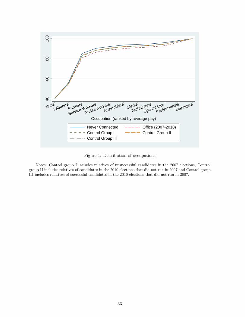
4060

8010

0

Special Occ.Managers

Professionals

TechniciansClerks

Service WorkersFarmers

Trades workers

AssemblersLaborersNone

Occupation (ranked by average pay)

Never Connected Office (2007-2010)Control Group I Control Group IIControl Group III

Figure 1: Distribution of occupations

Notes: Control group I includes relatives of unsuccessful candidates in the 2007 elections, Controlgroup II includes relatives of candidates in the 2010 elections that did not run in 2007 and Control groupIII includes relatives of successful candidates in the 2010 elections that did not run in 2007.

33

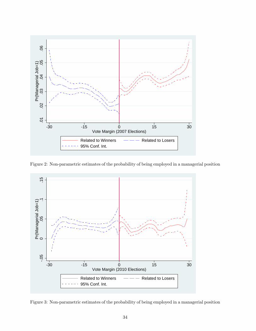
.01

.02

.03

.04

.05

.06

Pr(

Man

ager

ial J

ob=

1)

-30 -15 0 15 30Vote Margin (2007 Elections)

Related to Winners Related to Losers95% Conf. Int.

Figure 2: Non-parametric estimates of the probability of being employed in a managerial position

-.05

0.0

5.1

.15

Pr(

Man

ager

ial J

ob=

1)

-30 -15 0 15 30Vote Margin (2010 Elections)

Related to Winners Related to Losers95% Conf. Int.

Figure 3: Non-parametric estimates of the probability of being employed in a managerial position

34

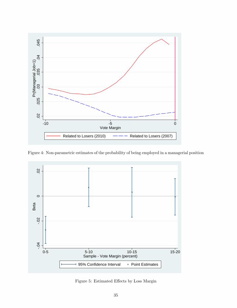
.02

.025

.03

.035

.04

.045

Pr(

Man

ager

ial J

ob=

1)

-10 -5 0Vote Margin

Related to Losers (2010) Related to Losers (2007)

Figure 4: Non-parametric estimates of the probability of being employed in a managerial position

-.04

-.02

0.0

2B

eta

0-5 5-10 10-15 15-20Sample - Vote Margin (percent)

95% Confidence Interval Point Estimates

Figure 5: Estimated Effects by Loss Margin

35

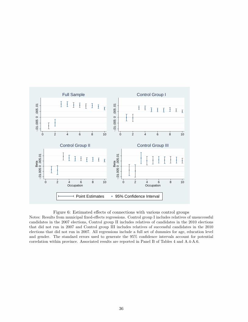
-.01

-.00

50

.005

.01

0 2 4 6 8 10

Full Sample

-.01

-.00

50

.005

.01

0 2 4 6 8 10

Control Group I

-.01

-.00

50

.005

.01

Bet

a

0 2 4 6 8 10Occupation

Control Group II

-.01

-.00

50

.005

.01

Bet

a

0 2 4 6 8 10Occupation

Control Group III

Point Estimates 95% Confidence Interval

Figure 6: Estimated effects of connections with various control groupsNotes: Results from municipal fixed-effects regressions. Control group I includes relatives of unsuccessfulcandidates in the 2007 elections, Control group II includes relatives of candidates in the 2010 electionsthat did not run in 2007 and Control group III includes relatives of successful candidates in the 2010elections that did not run in 2007. All regressions include a full set of dummies for age, education leveland gender. The standard errors used to generate the 95% confidence intervals account for potentialcorrelation within province. Associated results are reported in Panel B of Tables 4 and A.4-A.6.

36

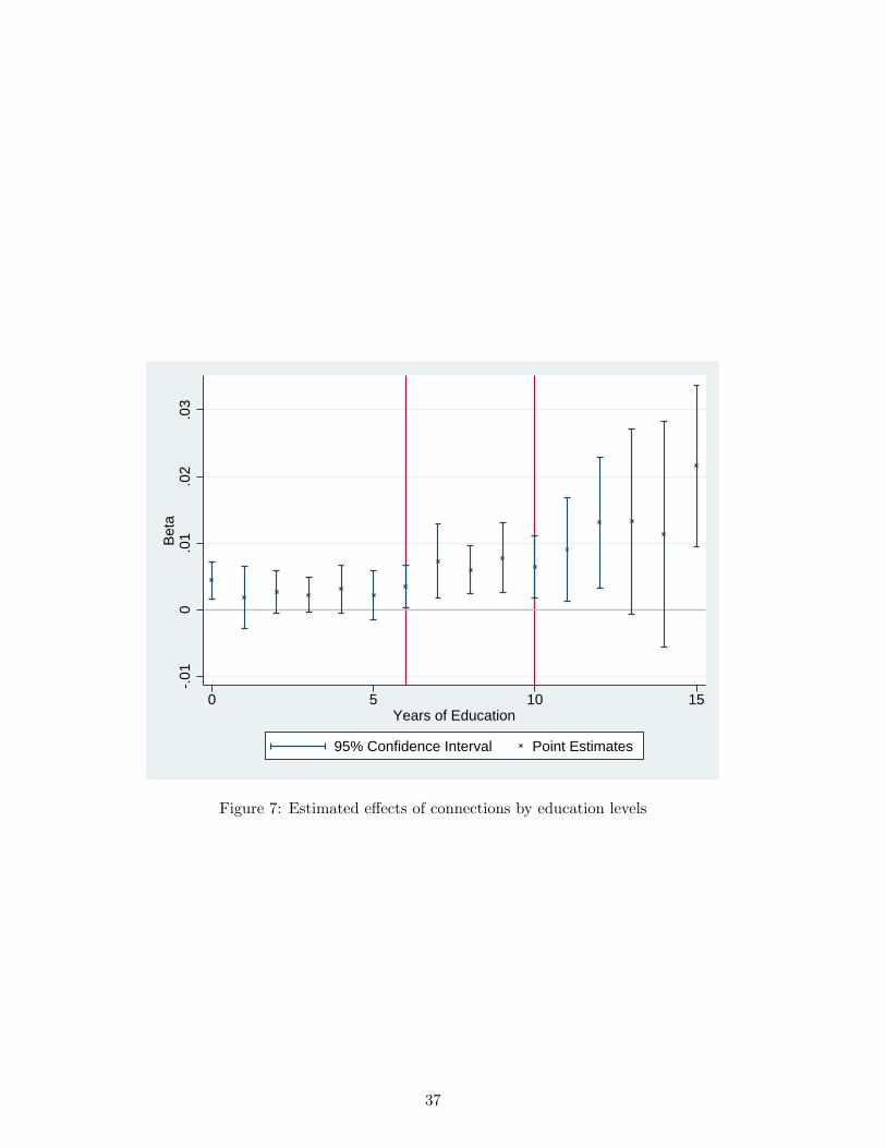
-.01

0.0

1.0

2.0

3B

eta

0 5 10 15Years of Education

95% Confidence Interval Point Estimates

Figure 7: Estimated effects of connections by education levels

37

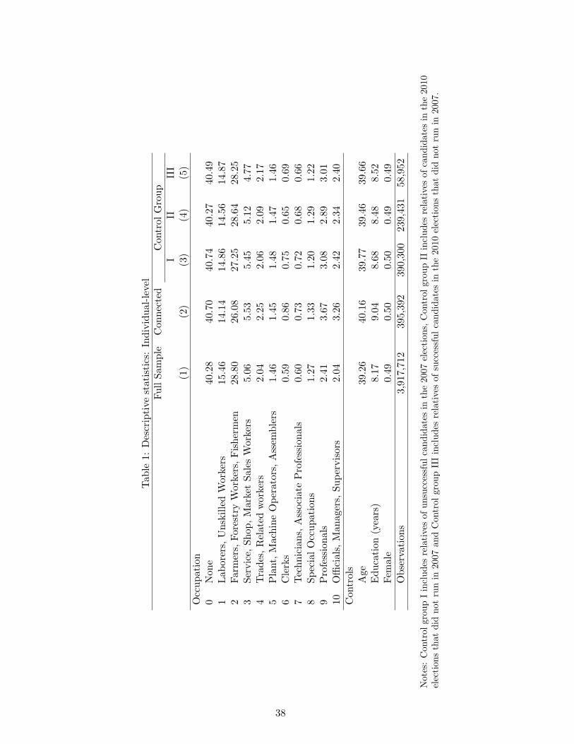
Tab

le1:

Des

crip

tive

stat

isti

cs:

Indi

vidu

al-l

evel

Full

Sam

ple

Con

nect

edC

ontr

olG

roup

III

III

(1)

(2)

(3)

(4)

(5)

Occ

upat

ion

0N

one

40.2

840

.70

40.7

440

.27

40.4

91

Lab

orer

s,U

nski

lled

Wor

kers

15.4

614

.14

14.8

614

.56

14.8

72

Farm

ers,

Fore

stry

Wor

kers

,F

ishe

rmen

28.8

026

.08

27.2

528

.64

28.2

53

Serv

ice,

Shop

,M

arke

tSa

les

Wor

kers

5.06

5.53

5.45

5.12

4.77

4T

rade

s,R

elat

edw

orke

rs2.

042.

252.

062.

092.

175

Pla

nt,

Mac

hine

Ope

rato

rs,

Ass

embl

ers

1.46

1.45

1.48

1.47

1.46

6C

lerk

s0.

590.

860.

750.

650.

697

Tec

hnic

ians

,A

ssoc

iate

Pro

fess

iona

ls0.

600.

730.

720.

680.

668

Spec

ial

Occ

upat

ions

1.27

1.33

1.20

1.29

1.22

9P

rofe

ssio

nals

2.41

3.67

3.08

2.89

3.01

10O

ffici

als,

Man

ager

s,Su

perv

isor

s2.

043.

262.

422.

342.

40C

ontr

ols

Age

39.2

640

.16

39.7

739

.46

39.6

6E

duca

tion

(yea

rs)

8.17

9.04

8.68

8.48

8.52

Fem

ale

0.49

0.50

0.50

0.49

0.49

Obs

erva

tion

s3,

917,

712

395,

392

390,

300

239,

431

58,9

52

Not

es:

Con

trol

grou

pI

incl

udes

rela

tive

sof

unsu

cces

sful

cand

idat

esin

the

2007

elec

tion

s,C

ontr

olgr

oup

IIin

clud

esre

lati

ves

ofca

ndid

ates

inth

e20

10el

ecti

ons

that

did

not

run

in20

07an

dC

ontr

olgr

oup

III

incl

udes

rela

tive

sof

succ

essf

ulca

ndid

ates

inth

e20

10el

ecti

ons

that

did

not

run

in20

07.

38

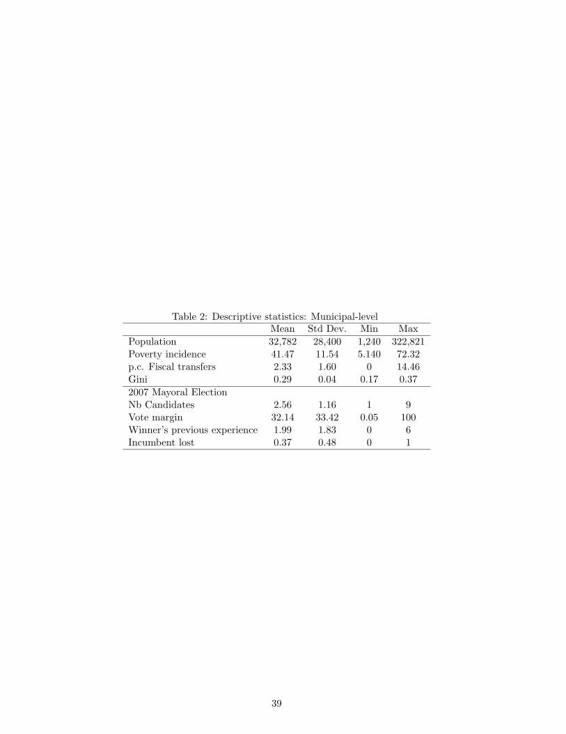
Table 2: Descriptive statistics: Municipal-levelMean Std Dev. Min Max

Population 32,782 28,400 1,240 322,821Poverty incidence 41.47 11.54 5.140 72.32p.c. Fiscal transfers 2.33 1.60 0 14.46Gini 0.29 0.04 0.17 0.372007 Mayoral ElectionNb Candidates 2.56 1.16 1 9Vote margin 32.14 33.42 0.05 100Winner’s previous experience 1.99 1.83 0 6Incumbent lost 0.37 0.48 0 1

39

Tab

le3:

The

effec

tsof

conn

ecti

ons

onth

epr

obab

ility

ofbe

ing

inan

yoc

cupa

tion

wit

hre

gres

sion

disc

onti

nuit

yde

sign

s-

Non

para

met

ric

(1)

(2)

(3)

(4)

(5)

(6)

(7)

(8)

(9)

(10)

1-10

2-10

3-10

4-10

5-10

6-10

7-10

8-10

9-10

10-

Pan

elA

:O

ptim

alB

andw

idth

Con

nect

edO

ffice

(200

7)0.

0106

0.07

40**

*0.

0961

***

0.08

30**

*0.

0778

***

0.08

30**

*0.

0723

***

0.06

69**

*0.

0742

***

0.01

25*

(0.0

25)

(0.0

28)

(0.0

18)

(0.0

15)

(0.0

15)

(0.0

16)

(0.0

14)

(0.0

15)

(0.0

15)

(0.0

07)

Obs

erva

tion

s30

,427

30,4

2730

,427

30,4

2730

,427

30,4

2730

,427

30,4

2730

,427

30,4

27P

anel

B:

Hal

fO

ptim

alB

andw

idth

Con

nect

edO

ffice

(200

7)0.

0446

0.12

99**

*0.

1317

***

0.11

93**

*0.

1072

***

0.09

46**

*0.

0796

***

0.06

96**

*0.

0573

***

0.01

67**

(0.0

37)

(0.0

37)

(0.0

23)

(0.0

20)

(0.0

19)

(0.0

18)

(0.0

16)

(0.0

18)

(0.0

19)

(0.0

08)

Obs

erva

tion

s30

,427

30,4

2730

,427

30,4

2730

,427

30,4

2730

,427

30,4

2730

,427

30,4

27P

anel

C:

Tw

ice

Opt

imal

Ban

dwid

thC

onne

cted

Offi

ce(2

007)

-0.0

129

0.00

680.

0569

***

0.05

13**

*0.

0406

***

0.04

35**

*0.

0403

***

0.04

42**

*0.

0399

***

0.01

24**

(0.0

18)

(0.0

19)

(0.0

13)

(0.0

12)

(0.0

11)

(0.0

11)

(0.0

11)

(0.0

11)

(0.0

11)

(0.0

06)

Obs

erva

tion

s30

,427

30,4

2730

,427

30,4

2730

,427

30,4

2730

,427

30,4

2730

,427

30,4

27

Not

es:

Res

ults

from

nonp

aram

etri

cre

gres

sion

s.T

hesa

mpl

ein

clud

esre

lati

ves

ofon

eof

the

top

two

cand

idat

esin

the

2007

may

oral

and

vice

-may

oral

elec

tion

s(v

ote

mar

gin

+/-

5pe

rcen

t).

The

depe

nden

tva

riab

leis

adu

mm

yeq

ual

toon

eif

the

indi

vidu

alis

empl

oyed

(Col

umn

1),

isem

ploy

edin

occu

pati

ons

2-10

(Col

umn

2),

isem

ploy

edin

occu

pati

ons

3-10

(Col

umn

3),

isem

ploy

edin

occu

pati

ons

4-10

(Col

umn

4),

isem

ploy

edin

occu

pati

ons

5-10

(Col

umn

5),i

sem

ploy

edin

occu

pati

ons

6-10

(Col

umn

6),i

sem

ploy

edin

occu

pati

ons

7-10

(Col

umn

7),i

sem

ploy

edin

occu

pati

ons

8-10

(Col

umn

8),

isem

ploy

edin

occu

pati

ons

9-10

(Col

umn

9)an

dis

empl

oyed

inoc

cupa

tion

10(C

olum

n10

).*

deno

tes

sign

ifica

nce

atth

e10

%,

**at

the

5%an

d,**

*at

the

1%le

vel.

40

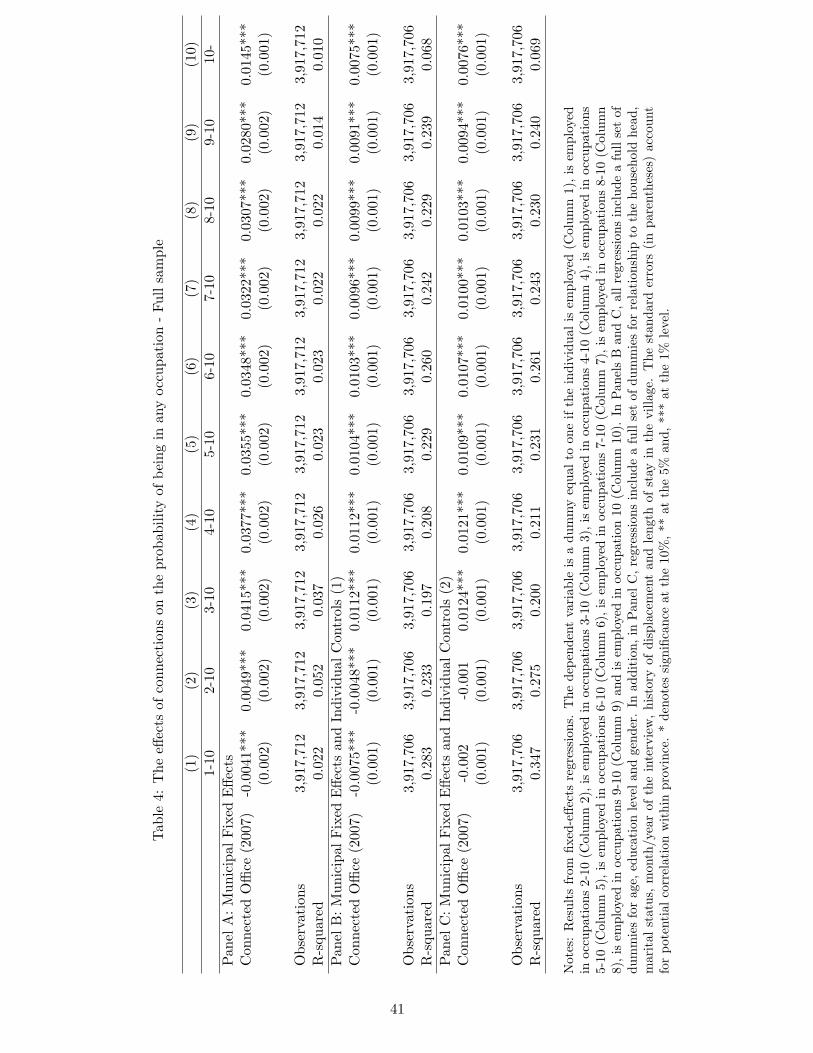
Tab

le4:

The

effec

tsof

conn

ecti

ons

onth

epr

obab

ility

ofbe

ing

inan

yoc

cupa

tion

-Fu

llsa

mpl

e

(1)

(2)

(3)

(4)

(5)

(6)

(7)

(8)

(9)

(10)

1-10

2-10

3-10

4-10

5-10

6-10

7-10

8-10

9-10

10-

Pan

elA

:M

unic

ipal

Fix

edE

ffect

sC

onne

cted

Offi

ce(2

007)

-0.0

041*

**0.

0049

***

0.04

15**

*0.

0377

***

0.03

55**

*0.

0348

***

0.03

22**

*0.

0307

***

0.02

80**

*0.

0145

***

(0.0

02)

(0.0

02)

(0.0

02)

(0.0

02)

(0.0

02)

(0.0

02)

(0.0

02)

(0.0

02)

(0.0

02)

(0.0

01)

Obs

erva

tion

s3,

917,

712

3,91

7,71

23,

917,

712

3,91

7,71

23,

917,

712

3,91

7,71

23,

917,

712

3,91

7,71

23,

917,

712

3,91

7,71

2R

-squ

ared

0.02

20.

052

0.03

70.

026

0.02

30.

023

0.02

20.

022

0.01

40.

010

Pan

elB

:M

unic

ipal

Fix

edE

ffect

san

dIn

divi

dual

Con

trol

s(1

)C

onne

cted

Offi

ce(2

007)

-0.0

075*

**-0

.004

8***

0.01

12**

*0.

0112

***

0.01

04**

*0.

0103

***

0.00

96**

*0.

0099

***

0.00

91**

*0.

0075

***

(0.0

01)

(0.0

01)

(0.0

01)

(0.0

01)

(0.0

01)

(0.0

01)

(0.0

01)

(0.0

01)

(0.0

01)

(0.0

01)

Obs

erva

tion

s3,

917,

706

3,91

7,70

63,

917,

706

3,91

7,70

63,

917,

706

3,91

7,70

63,

917,

706

3,91

7,70

63,

917,

706

3,91

7,70

6R

-squ

ared

0.28

30.

233

0.19

70.

208

0.22

90.

260

0.24

20.

229

0.23

90.

068

Pan

elC

:M

unic

ipal

Fix

edE

ffect

san

dIn

divi

dual

Con

trol

s(2

)C

onne

cted

Offi

ce(2

007)

-0.0

02-0

.001

0.01

24**

*0.

0121

***

0.01

09**

*0.

0107

***

0.01

00**

*0.

0103

***

0.00

94**

*0.

0076

***

(0.0

01)

(0.0

01)

(0.0

01)

(0.0

01)

(0.0

01)

(0.0

01)

(0.0

01)

(0.0

01)

(0.0

01)

(0.0

01)

Obs

erva

tion

s3,

917,

706

3,91

7,70

63,

917,

706

3,91

7,70

63,

917,

706

3,91

7,70

63,

917,

706

3,91

7,70

63,

917,

706

3,91

7,70

6R

-squ

ared

0.34

70.

275

0.20

00.

211

0.23

10.

261

0.24

30.

230

0.24

00.

069

Not

es:

Res

ults

from

fixed

-effe

cts

regr

essi

ons.

The

depe

nden

tva

riab

leis

adu

mm

yeq

ual

toon

eif

the

indi

vidu

alis

empl

oyed

(Col

umn

1),

isem

ploy

edin

occu

pati

ons

2-10

(Col

umn

2),i

sem

ploy

edin

occu

pati

ons

3-10

(Col

umn

3),i

sem

ploy

edin

occu

pati

ons

4-10

(Col

umn

4),i

sem

ploy

edin

occu

pati

ons

5-10

(Col

umn

5),i

sem

ploy

edin

occu

pati

ons

6-10

(Col

umn

6),i

sem

ploy

edin

occu

pati

ons

7-10

(Col

umn

7),i

sem

ploy

edin

occu

pati

ons

8-10

(Col

umn

8),i

sem

ploy

edin

occu

pati

ons

9-10

(Col

umn

9)an

dis

empl

oyed

inoc

cupa

tion

10(C

olum

n10

).In

Pan

els

Ban

dC

,all

regr

essi

ons

incl

ude

afu

llse

tof

dum

mie

sfo

rag

e,ed

ucat

ion

leve

land

gend

er.

Inad

diti

on,i

nP

anel

C,r

egre

ssio

nsin

clud

ea

full

set

ofdu

mm

ies

for

rela

tion

ship

toth

eho

useh

old

head

,m

arit

alst

atus

,m

onth

/yea

rof

the

inte

rvie

w,

hist

ory

ofdi

spla

cem

ent

and

leng

thof

stay

inth

evi

llage

.T

hest

anda

rder

rors

(in

pare

nthe

ses)

acco

unt

for

pote

ntia

lco

rrel

atio

nw

ithi

npr

ovin

ce.

*de

note

ssi

gnifi

canc

eat

the

10%

,**

atth

e5%

and,

***

atth

e1%

leve

l.

41

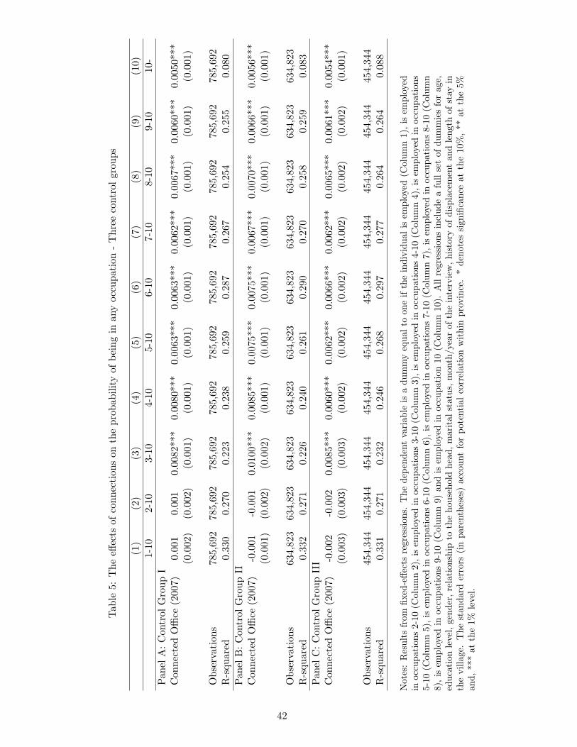
Tab

le5:

The

effec

tsof

conn

ecti

ons

onth

epr

obab

ility

ofbe

ing

inan

yoc

cupa

tion

-T

hree

cont

rol

grou

ps

(1)

(2)

(3)

(4)

(5)

(6)

(7)

(8)

(9)

(10)

1-10

2-10

3-10

4-10

5-10

6-10

7-10

8-10

9-10

10-

Pan

elA

:C

ontr

olG

roup

IC

onne

cted

Offi

ce(2

007)

0.00

10.

001

0.00

82**

*0.

0080

***

0.00

63**

*0.

0063

***

0.00

62**

*0.

0067

***

0.00

60**

*0.

0050

***

(0.0

02)

(0.0

02)

(0.0

01)

(0.0

01)

(0.0

01)

(0.0

01)

(0.0

01)

(0.0

01)

(0.0

01)

(0.0

01)

Obs

erva

tion

s78

5,69

278

5,69

278

5,69

278

5,69

278

5,69

278

5,69

278

5,69

278

5,69

278

5,69

278

5,69

2R

-squ

ared

0.33

00.

270

0.22

30.

238

0.25

90.

287

0.26

70.

254

0.25

50.

080

Pan

elB

:C

ontr

olG

roup

IIC

onne

cted

Offi

ce(2

007)

-0.0

01-0

.001

0.01

00**

*0.

0085

***

0.00

75**

*0.

0075

***

0.00

67**

*0.

0070

***

0.00

66**

*0.

0056

***

(0.0

01)

(0.0

02)

(0.0

02)

(0.0

01)

(0.0

01)

(0.0

01)

(0.0

01)

(0.0

01)

(0.0

01)

(0.0

01)

Obs

erva

tion

s63

4,82

363

4,82

363

4,82

363

4,82

363

4,82

363

4,82

363

4,82

363

4,82

363

4,82

363

4,82

3R

-squ

ared

0.33

20.

271

0.22

60.

240

0.26

10.

290

0.27

00.

258

0.25

90.

083

Pan

elC

:C

ontr

olG

roup

III

Con

nect

edO

ffice

(200

7)-0

.002

-0.0

020.

0085

***

0.00

60**

*0.

0062

***

0.00

66**

*0.

0062

***

0.00

65**

*0.

0061

***

0.00

54**

*(0

.003

)(0

.003

)(0

.003

)(0

.002

)(0

.002

)(0

.002

)(0

.002

)(0

.002

)(0

.002

)(0

.001

)

Obs

erva

tion

s45

4,34

445

4,34

445

4,34

445

4,34

445

4,34

445

4,34

445

4,34

445

4,34

445

4,34

445

4,34

4R

-squ

ared

0.33

10.

271

0.23

20.

246

0.26

80.

297

0.27

70.

264

0.26

40.

088

Not

es:

Res

ults

from

fixed

-effe

cts

regr

essi

ons.

The

depe

nden

tva

riab

leis

adu

mm

yeq

ual

toon

eif

the

indi

vidu

alis

empl

oyed

(Col

umn

1),

isem

ploy

edin

occu

pati

ons

2-10

(Col

umn

2),i

sem

ploy

edin

occu

pati

ons

3-10

(Col

umn

3),i

sem

ploy

edin

occu

pati

ons

4-10

(Col

umn

4),i

sem

ploy

edin

occu

pati

ons

5-10

(Col

umn

5),i

sem

ploy

edin

occu

pati

ons

6-10

(Col

umn

6),i

sem

ploy

edin

occu

pati

ons

7-10

(Col

umn

7),i

sem

ploy

edin

occu

pati

ons

8-10

(Col

umn

8),

isem

ploy

edin

occu

pati

ons

9-10

(Col

umn

9)an

dis

empl

oyed

inoc

cupa

tion

10(C

olum

n10

).A

llre

gres

sion

sin

clud

ea

full

set

ofdu

mm

ies

for

age,

educ

atio

nle

vel,

gend

er,r

elat

ions

hip

toth

eho

useh

old

head

,mar

ital

stat

us,m

onth

/yea

rof

the

inte

rvie

w,h

isto

ryof

disp

lace

men

tan

dle

ngth

ofst

ayin

the

villa

ge.

The

stan

dard

erro

rs(i

npa

rent

hese

s)ac

coun

tfo

rpo

tent

ial

corr

elat

ion

wit

hin

prov

ince

.*

deno

tes

sign

ifica

nce

atth

e10

%,

**at

the

5%an

d,**

*at

the

1%le

vel.

42

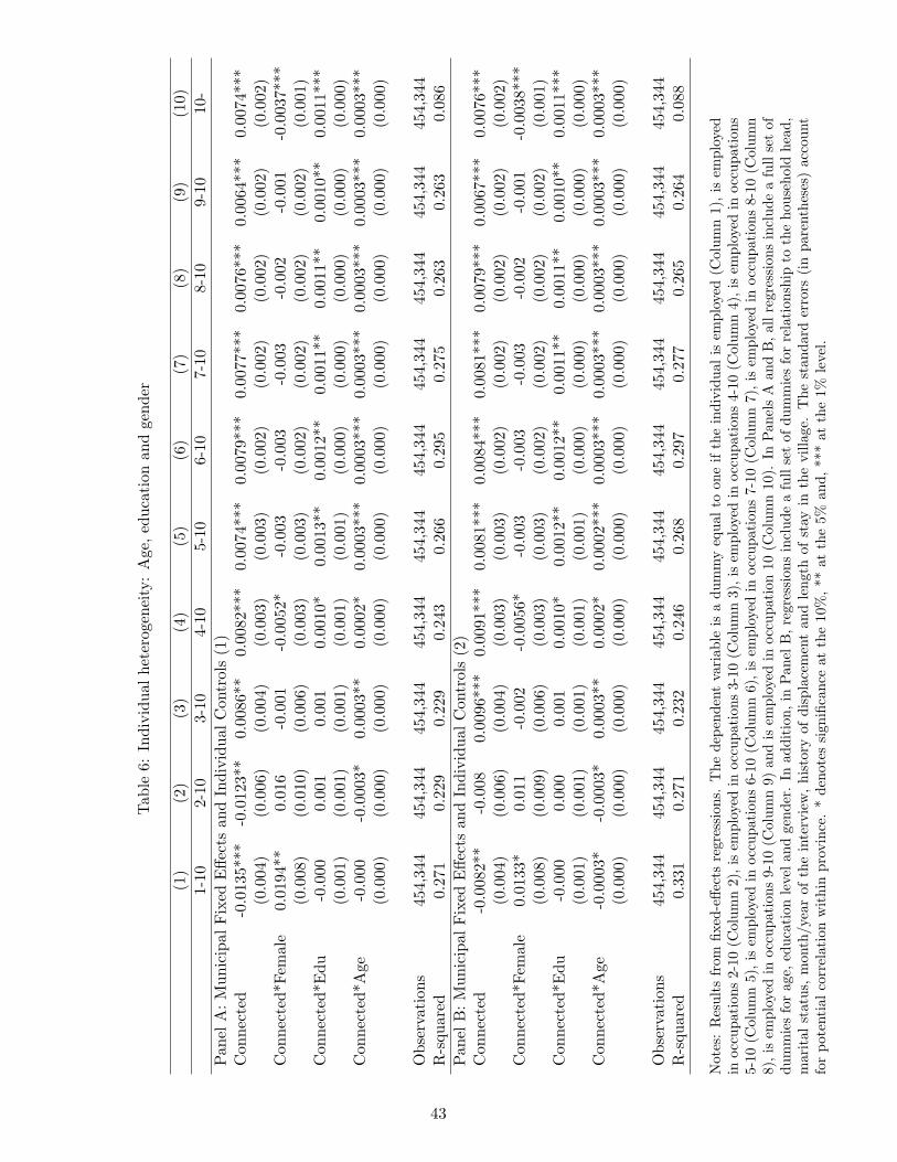
Tab

le6:

Indi

vidu

alhe

tero

gene

ity:

Age

,ed

ucat

ion

and

gend

er

(1)

(2)

(3)

(4)

(5)

(6)

(7)

(8)

(9)

(10)

1-10

2-10

3-10

4-10

5-10

6-10

7-10

8-10

9-10

10-

Pan

elA

:M

unic

ipal

Fix

edE

ffect

san

dIn

divi

dual

Con

trol

s(1

)C

onne

cted

-0.0

135*

**-0

.012

3**

0.00

86**

0.00

82**

*0.

0074

***

0.00

79**

*0.

0077

***

0.00

76**

*0.

0064

***

0.00

74**

*(0

.004

)(0

.006

)(0

.004

)(0

.003

)(0

.003

)(0

.002

)(0

.002

)(0

.002

)(0

.002

)(0

.002

)C

onne

cted

*Fem

ale

0.01

94**

0.01

6-0

.001

-0.0

052*

-0.0

03-0

.003

-0.0

03-0

.002

-0.0

01-0

.003

7***

(0.0

08)

(0.0

10)

(0.0

06)

(0.0

03)

(0.0

03)

(0.0

02)

(0.0

02)

(0.0

02)

(0.0

02)

(0.0

01)

Con

nect

ed*E

du-0

.000

0.00

10.

001

0.00

10*

0.00

13**

0.00

12**

0.00

11**

0.00

11**

0.00

10**

0.00

11**

*(0

.001

)(0

.001

)(0

.001

)(0

.001

)(0

.001

)(0

.000

)(0

.000

)(0

.000

)(0

.000

)(0

.000

)C

onne

cted

*Age

-0.0

00-0

.000

3*0.

0003

**0.

0002

*0.

0003

***

0.00

03**

*0.

0003

***

0.00

03**

*0.

0003

***

0.00

03**

*(0

.000

)(0

.000

)(0

.000

)(0

.000

)(0

.000

)(0

.000

)(0

.000

)(0

.000

)(0

.000

)(0

.000

)

Obs

erva

tion

s45

4,34

445

4,34

445

4,34

445

4,34

445

4,34

445

4,34

445

4,34

445

4,34

445

4,34

445

4,34

4R

-squ

ared

0.27

10.

229

0.22

90.

243

0.26

60.

295

0.27

50.

263

0.26

30.

086

Pan

elB

:M

unic

ipal

Fix

edE

ffect

san

dIn

divi

dual

Con

trol

s(2

)C

onne

cted

-0.0

082*

*-0

.008

0.00

96**

*0.

0091

***

0.00

81**

*0.

0084

***

0.00

81**

*0.

0079

***

0.00

67**

*0.

0076

***

(0.0

04)

(0.0

06)

(0.0

04)

(0.0

03)

(0.0

03)

(0.0

02)

(0.0

02)

(0.0

02)

(0.0

02)

(0.0

02)

Con

nect

ed*F

emal

e0.

0133

*0.

011

-0.0

02-0

.005

6*-0

.003

-0.0

03-0

.003

-0.0

02-0

.001

-0.0

038*

**(0

.008

)(0

.009

)(0

.006

)(0

.003

)(0

.003

)(0

.002

)(0

.002

)(0

.002

)(0

.002

)(0

.001

)C

onne

cted

*Edu

-0.0

000.

000

0.00

10.

0010

*0.

0012

**0.

0012

**0.

0011

**0.

0011

**0.

0010

**0.

0011

***

(0.0

01)

(0.0

01)

(0.0

01)

(0.0

01)

(0.0

01)

(0.0

00)

(0.0

00)

(0.0

00)

(0.0

00)

(0.0

00)

Con

nect

ed*A

ge-0

.000

3*-0

.000

3*0.

0003

**0.

0002

*0.

0002

***

0.00

03**

*0.

0003

***

0.00

03**

*0.

0003

***

0.00

03**

*(0

.000

)(0

.000

)(0

.000

)(0

.000

)(0

.000

)(0

.000

)(0

.000

)(0

.000

)(0

.000

)(0

.000

)

Obs

erva

tion

s45

4,34

445

4,34

445

4,34

445

4,34

445

4,34

445

4,34

445

4,34

445

4,34

445

4,34

445

4,34

4R

-squ

ared

0.33

10.

271

0.23

20.

246

0.26

80.

297

0.27

70.

265

0.26

40.

088

Not

es:

Res

ults

from

fixed

-effe

cts

regr

essi

ons.

The

depe

nden

tva

riab

leis

adu

mm

yeq

ual

toon

eif

the

indi

vidu

alis

empl

oyed

(Col

umn

1),

isem

ploy

edin

occu

pati

ons

2-10

(Col

umn

2),i

sem

ploy

edin

occu

pati

ons

3-10

(Col

umn

3),i

sem

ploy

edin

occu

pati

ons

4-10

(Col

umn

4),i

sem

ploy

edin

occu

pati

ons

5-10

(Col

umn

5),i

sem

ploy

edin

occu

pati

ons

6-10

(Col

umn

6),i

sem

ploy

edin

occu

pati

ons

7-10

(Col

umn

7),i

sem

ploy

edin

occu

pati

ons

8-10

(Col

umn

8),i

sem

ploy

edin

occu

pati

ons

9-10

(Col

umn

9)an

dis

empl

oyed

inoc

cupa

tion

10(C

olum

n10

).In

Pan

els

Aan

dB

,all

regr

essi

ons

incl

ude

afu

llse

tof

dum

mie

sfo

rag

e,ed

ucat

ion

leve

land

gend

er.

Inad

diti

on,i

nP

anel

B,r

egre

ssio

nsin

clud

ea

full

set

ofdu

mm

ies

for

rela

tion

ship

toth

eho

useh

old

head

,m

arit

alst

atus

,m

onth

/yea

rof

the

inte

rvie

w,

hist

ory

ofdi

spla

cem

ent

and

leng

thof

stay

inth

evi

llage

.T

hest

anda

rder

rors

(in

pare

nthe

ses)

acco

unt

for

pote

ntia

lco

rrel

atio

nw

ithi

npr

ovin

ce.

*de

note

ssi

gnifi

canc

eat

the

10%

,**

atth

e5%

and,

***

atth

e1%

leve

l.

43

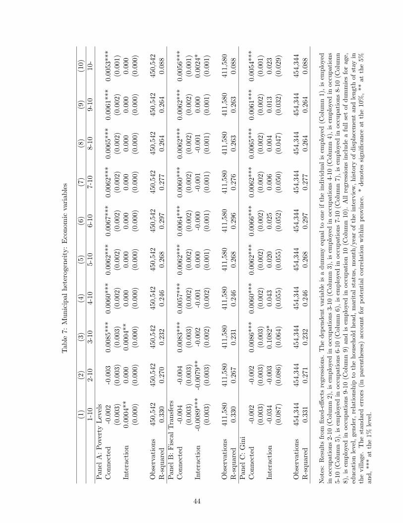
Tab

le7:

Mun

icip

alhe

tero

gene

ity:

Eco

nom

icva

riab

les

(1)

(2)

(3)

(4)

(5)

(6)

(7)

(8)

(9)

(10)

1-10

2-10

3-10

4-10

5-10

6-10

7-10

8-10

9-10

10-

Pan

elA

:P

over

tyL

evel

sC

onne

cted

-0.0

02-0

.003

0.00

85**

*0.

0060

***

0.00

62**

*0.

0067

***

0.00

62**

*0.

0065

***

0.00

61**

*0.

0053

***

(0.0

03)

(0.0

03)

(0.0

03)

(0.0

02)

(0.0

02)

(0.0

02)

(0.0

02)

(0.0

02)

(0.0

02)

(0.0

01)

Inte

ract

ion

0.00

04**

0.00

00.

0004

**0.

000

0.00

00.

000

0.00

00.

000

0.00

00.

000

(0.0

00)

(0.0

00)

(0.0

00)

(0.0

00)

(0.0

00)

(0.0

00)

(0.0

00)

(0.0

00)

(0.0

00)

(0.0

00)

Obs

erva

tion

s45

0,54

245

0,54

245

0,54

245

0,54

245

0,54

245

0,54

245

0,54

245

0,54

245

0,54

245

0,54

2R

-squ

ared

0.33

00.

270

0.23

20.

246

0.26

80.

297

0.27

70.

264

0.26

40.

088

Pan

elB

:F

isca

lT

rans

fers

Con

nect

ed-0

.004

-0.0

040.

0083

***

0.00

57**

*0.

0062

***

0.00

64**

*0.

0060

***

0.00

62**

*0.

0062

***

0.00

56**

*(0

.003

)(0

.003

)(0

.003

)(0

.002

)(0

.002

)(0

.002

)(0

.002

)(0

.002

)(0

.002

)(0

.001

)In

tera

ctio

n-0

.008

9***

-0.0

079*

*-0

.002

-0.0

010.

000

-0.0

00-0

.001

-0.0

010.

000

0.00

24*

(0.0

03)

(0.0

03)

(0.0

02)

(0.0

02)

(0.0

01)

(0.0

01)

(0.0

01)

(0.0

01)

(0.0

01)

(0.0

01)

Obs

erva

tion

s41

1,58

041

1,58

041

1,58

041

1,58

041

1,58

041

1,58

041

1,58

041

1,58

041

1,58

041

1,58

0R

-squ

ared

0.33

00.

267

0.23

10.

246

0.26

80.

296

0.27

60.

263

0.26

30.

088

Pan

elC

:G

ini

Con

nect

ed-0

.002

-0.0

020.

0086

***

0.00

60**

*0.

0062

***

0.00

66**

*0.

0062

***

0.00

65**

*0.

0061

***

0.00

54**

*(0

.003

)(0

.003

)(0

.003

)(0

.002

)(0

.002

)(0

.002

)(0

.002

)(0

.002

)(0

.002

)(0

.001

)In

tera

ctio

n-0

.034

-0.0

030.

1082

*0.

043

0.02

00.

025

0.00

60.

004

0.01

30.

023

(0.0

87)

(0.0

86)

(0.0

64)

(0.0

55)

(0.0

55)

(0.0

52)

(0.0

50)

(0.0

47)

(0.0

32)

(0.0

29)

Obs

erva

tion

s45

4,34

445

4,34

445

4,34

445

4,34

445

4,34

445

4,34

445

4,34

445

4,34

445

4,34

445

4,34

4R

-squ

ared

0.33

10.

271

0.23

20.

246

0.26

80.

297

0.27

70.

264

0.26

40.

088

Not

es:

Res

ults

from

fixed

-effe

cts

regr

essi

ons.

The

depe

nden

tva

riab

leis

adu

mm

yeq

ual

toon

eif

the

indi

vidu

alis

empl

oyed

(Col

umn

1),

isem

ploy

edin

occu

pati

ons

2-10

(Col

umn

2),i

sem

ploy

edin

occu

pati

ons

3-10

(Col

umn

3),i

sem

ploy

edin

occu

pati

ons

4-10

(Col

umn

4),i

sem

ploy

edin

occu

pati

ons

5-10

(Col

umn

5),i

sem

ploy

edin

occu

pati

ons

6-10

(Col

umn

6),i

sem

ploy

edin

occu

pati

ons

7-10

(Col

umn

7),i

sem

ploy

edin

occu

pati

ons

8-10

(Col

umn

8),

isem

ploy

edin

occu

pati

ons

9-10

(Col

umn

9)an

dis

empl

oyed

inoc

cupa

tion

10(C

olum

n10

).A

llre

gres

sion

sin

clud

ea

full

set

ofdu

mm

ies

for

age,

educ

atio

nle

vel,

gend

er,r

elat

ions

hip

toth

eho

useh

old

head

,mar

ital

stat

us,m

onth

/yea

rof

the

inte

rvie

w,h

isto

ryof

disp

lace

men

tan

dle

ngth

ofst

ayin

the

villa

ge.

The

stan

dard

erro

rs(i

npa

rent

hese

s)ac

coun

tfo

rpo

tent

ial

corr

elat

ion

wit

hin

prov

ince

.*

deno

tes

sign

ifica

nce

atth

e10

%,

**at

the

5%an

d,**

*at

the

1%le

vel.

44

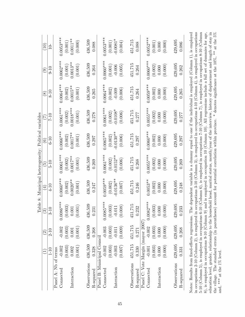
Tab

le8:

Mun

icip

alhe

tero

gene

ity:

Pol

itic

alva

riab

les

(1)

(2)

(3)

(4)

(5)

(6)

(7)

(8)

(9)

(10)

1-10

2-10

3-10

4-10

5-10

6-10

7-10

8-10

9-10

10-

Pan

elA

:N

bof

term

sC

onne

cted

-0.0

02-0

.002

0.00

86**

*0.

0060

***

0.00

61**

*0.

0066

***

0.00

61**

*0.

0064

***

0.00

62**

*0.

0053

***

(0.0

03)

(0.0

03)

(0.0

03)

(0.0

02)

(0.0

02)

(0.0

02)

(0.0

02)

(0.0

02)

(0.0

01)

(0.0

01)

Inte

ract

ion

0.00

20.

001

0.00

10.

0020

**0.

0017

**0.

0017

**0.

0018

***

0.00

15**

0.00

13**

0.00

11**

(0.0

01)

(0.0

01)

(0.0

01)

(0.0

01)

(0.0

01)

(0.0

01)

(0.0

01)

(0.0

01)

(0.0

01)

(0.0

00)

Obs

erva

tion

s43

6,50

943

6,50

943

6,50

943

6,50

943

6,50

943

6,50

943

6,50

943

6,50

943

6,50

943

6,50

9R

-squ

ared

0.32

80.

268

0.23

10.

247

0.26

90.

297

0.27

80.

265

0.26

40.

088

Pan

elB

:M

unic

ipal

Cou

ncil

Con

nect

ed-0

.002

-0.0

030.

0085

***

0.00

59**

*0.

0061

***

0.00

65**

*0.

0061

***

0.00

64**

*0.

0060

***

0.00

53**

*(0

.003

)(0

.003

)(0

.003

)(0

.002

)(0

.002

)(0

.002

)(0

.002

)(0

.002

)(0

.001

)(0

.001

)In

tera

ctio

n-0

.003

-0.0

11-0

.011

-0.0

136*

*-0

.015

2**

-0.0

130*

*-0

.010

8*-0

.009

-0.0

06-0

.008

1*(0

.007

)(0

.009

)(0

.008

)(0

.007

)(0

.006

)(0

.006

)(0

.006

)(0

.006

)(0

.005

)(0

.004

)

Obs

erva

tion

s45

1,71

545

1,71

545

1,71

545

1,71

545

1,71

545

1,71

545

1,71

545

1,71

545

1,71

545

1,71

5R

-squ

ared

0.33

00.

271

0.23

20.

246

0.26

80.

297

0.27

70.

264

0.26

40.

088

Pan

elC

:V

ote

Mar

gin

(may

or20

07)

Con

nect

ed-0

.001

-0.0

020.

0082

***

0.00

53**

0.00

55**

*0.

0060

***

0.00

55**

*0.

0059

***

0.00

60**

*0.

0052

***

(0.0

03)

(0.0

03)

(0.0

03)

(0.0

02)

(0.0

02)

(0.0

02)

(0.0

02)

(0.0

02)

(0.0

02)

(0.0

01)

Inte

ract

ion

0.00

00.

000

0.00

00.

000

0.00

00.

000

0.00

00.

000

0.00

00.

000

(0.0

00)

(0.0

00)

(0.0

00)

(0.0

00)

(0.0

00)

(0.0

00)

(0.0

00)

(0.0

00)

(0.0

00)

(0.0

00)

Obs

erva

tion

s42

9,69

542

9,69

542

9,69

542

9,69

542

9,69

542

9,69

542

9,69

542

9,69

542

9,69

542

9,69

5R

-squ

ared

0.33

10.

268

0.23

30.

248

0.26

90.

297

0.27

70.

265

0.26

20.

086

Not

es:

Res

ults

from

fixed

-effe

cts

regr

essi

ons.

The

depe

nden

tva

riab

leis

adu

mm

yeq

ual

toon

eif

the

indi

vidu

alis

empl

oyed

(Col

umn

1),

isem

ploy

edin

occu

pati

ons

2-10

(Col

umn

2),i

sem

ploy

edin

occu

pati

ons

3-10

(Col

umn

3),i

sem

ploy

edin

occu

pati

ons

4-10

(Col

umn

4),i

sem

ploy

edin

occu

pati

ons

5-10

(Col

umn

5),i

sem

ploy

edin

occu

pati

ons

6-10

(Col

umn

6),i

sem

ploy

edin

occu

pati

ons

7-10

(Col

umn

7),i

sem

ploy

edin

occu

pati

ons

8-10

(Col

umn

8),

isem

ploy

edin

occu

pati

ons

9-10

(Col

umn

9)an

dis

empl

oyed

inoc

cupa

tion

10(C

olum

n10

).A

llre

gres

sion

sin

clud

ea

full

set

ofdu

mm

ies

for

age,

educ

atio

nle

vel,

gend

er,r

elat

ions

hip

toth

eho

useh

old

head

,mar

ital

stat

us,m

onth

/yea

rof

the

inte

rvie

w,h

isto

ryof

disp

lace

men

tan

dle

ngth

ofst

ayin

the

villa

ge.

The

stan

dard

erro

rs(i

npa

rent

hese

s)ac

coun

tfo

rpo

tent

ial

corr

elat

ion

wit

hin

prov

ince

.*

deno

tes

sign

ifica

nce

atth

e10

%,

**at

the

5%an

d,**

*at

the

1%le

vel.

45

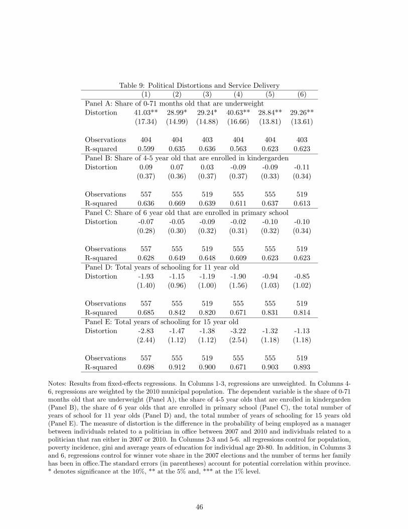
Table 9: Political Distortions and Service Delivery(1) (2) (3) (4) (5) (6)

Panel A: Share of 0-71 months old that are underweightDistortion 41.03** 28.99* 29.24* 40.63** 28.84** 29.26**

(17.34) (14.99) (14.88) (16.66) (13.81) (13.61)

Observations 404 404 403 404 404 403R-squared 0.599 0.635 0.636 0.563 0.623 0.623Panel B: Share of 4-5 year old that are enrolled in kindergardenDistortion 0.09 0.07 0.03 -0.09 -0.09 -0.11

(0.37) (0.36) (0.37) (0.37) (0.33) (0.34)

Observations 557 555 519 555 555 519R-squared 0.636 0.669 0.639 0.611 0.637 0.613Panel C: Share of 6 year old that are enrolled in primary schoolDistortion -0.07 -0.05 -0.09 -0.02 -0.10 -0.10

(0.28) (0.30) (0.32) (0.31) (0.32) (0.34)

Observations 557 555 519 555 555 519R-squared 0.628 0.649 0.648 0.609 0.623 0.623Panel D: Total years of schooling for 11 year oldDistortion -1.93 -1.15 -1.19 -1.90 -0.94 -0.85

(1.40) (0.96) (1.00) (1.56) (1.03) (1.02)

Observations 557 555 519 555 555 519R-squared 0.685 0.842 0.820 0.671 0.831 0.814Panel E: Total years of schooling for 15 year oldDistortion -2.83 -1.47 -1.38 -3.22 -1.32 -1.13

(2.44) (1.12) (1.12) (2.54) (1.18) (1.18)

Observations 557 555 519 555 555 519R-squared 0.698 0.912 0.900 0.671 0.903 0.893

Notes: Results from fixed-effects regressions. In Columns 1-3, regressions are unweighted. In Columns 4-6, regressions are weighted by the 2010 municipal population. The dependent variable is the share of 0-71months old that are underweight (Panel A), the share of 4-5 year olds that are enrolled in kindergarden(Panel B), the share of 6 year olds that are enrolled in primary school (Panel C), the total number ofyears of school for 11 year olds (Panel D) and, the total number of years of schooling for 15 years old(Panel E). The measure of distortion is the difference in the probability of being employed as a managerbetween individuals related to a politician in office between 2007 and 2010 and individuals related to apolitician that ran either in 2007 or 2010. In Columns 2-3 and 5-6. all regressions control for population,poverty incidence, gini and average years of education for individual age 20-80. In addition, in Columns 3and 6, regressions control for winner vote share in the 2007 elections and the number of terms her familyhas been in office.The standard errors (in parentheses) account for potential correlation within province.* denotes significance at the 10%, ** at the 5% and, *** at the 1% level.

46

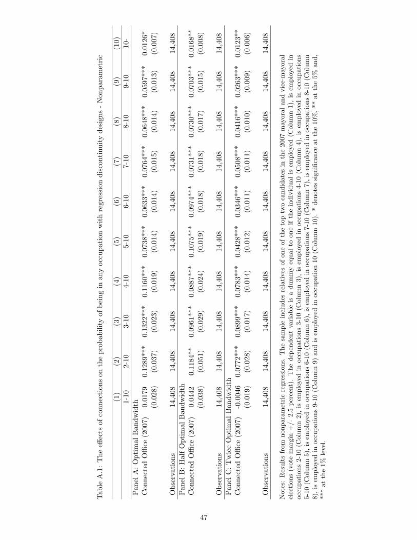
Tab

leA

.1:

The

effec

tsof

conn

ecti

ons

onth

epr

obab

ility

ofbe

ing

inan

yoc

cupa

tion

wit

hre

gres

sion

disc

onti

nuit

yde

sign

s-

Non

para

met

ric

(1)

(2)

(3)

(4)

(5)

(6)

(7)

(8)

(9)

(10)

1-10

2-10

3-10

4-10

5-10

6-10

7-10

8-10

9-10

10-

Pan

elA

:O

ptim

alB

andw

idth

Con

nect

edO

ffice

(200

7)0.

0179

0.12

89**

*0.

1322

***

0.11

60**

*0.

0738

***

0.06

33**

*0.

0764

***

0.06

48**

*0.

0597

***

0.01

26*

(0.0

28)

(0.0

37)

(0.0

23)

(0.0

19)

(0.0

14)

(0.0

14)

(0.0

15)

(0.0

14)

(0.0

13)

(0.0

07)

Obs

erva

tion

s14

,408

14,4

0814

,408

14,4

0814

,408

14,4

0814

,408

14,4

0814

,408

14,4

08P

anel

B:

Hal

fO

ptim

alB

andw

idth

Con

nect

edO

ffice

(200

7)0.

0442

0.11

84**

0.09

61**

*0.

0887

***

0.10

75**

*0.

0974

***

0.07

31**

*0.

0730

***

0.07

03**

*0.

0168

**(0

.038

)(0

.051

)(0

.029

)(0

.024

)(0

.019

)(0

.018

)(0

.018

)(0

.017

)(0

.015

)(0

.008

)

Obs

erva

tion

s14

,408

14,4

0814

,408

14,4

0814

,408

14,4

0814

,408

14,4

0814

,408

14,4

08P

anel

C:

Tw

ice

Opt

imal

Ban

dwid

thC

onne

cted

Offi

ce(2

007)

-0.0

046

0.07

72**

*0.

0899

***

0.07

83**

*0.

0428

***

0.03

46**

*0.

0508

***

0.04

16**

*0.

0263

***

0.01

23**

(0.0

19)

(0.0

28)

(0.0

17)

(0.0

14)

(0.0

12)

(0.0

11)

(0.0

11)

(0.0

10)

(0.0

09)

(0.0

06)

Obs

erva

tion

s14

,408

14,4

0814

,408

14,4

0814

,408

14,4

0814

,408

14,4

0814

,408

14,4

08

Not

es:

Res

ults

from

nonp

aram

etri

cre

gres

sion

s.T

hesa

mpl

ein

clud

esre

lati

ves

ofon

eof

the

top

two

cand

idat

esin

the

2007

may

oral

and

vice

-may

oral

elec

tion

s(v

ote

mar

gin

+/-

2.5

perc

ent)

.T

hede

pend

ent

vari

able

isa

dum

my

equa

lto

one

ifth

ein

divi

dual

isem

ploy

ed(C

olum

n1)

,is

empl

oyed

inoc

cupa

tion

s2-

10(C

olum

n2)

,is

empl

oyed

inoc

cupa

tion

s3-

10(C

olum

n3)

,is

empl

oyed

inoc

cupa

tion

s4-

10(C

olum

n4)

,is

empl

oyed

inoc

cupa

tion

s5-

10(C

olum

n5)

,is

empl

oyed

inoc

cupa

tion

s6-

10(C

olum

n6)

,is

empl

oyed

inoc

cupa

tion

s7-

10(C

olum

n7)

,is

empl

oyed

inoc

cupa

tion

s8-

10(C

olum

n8)

,is

empl

oyed

inoc

cupa

tion

s9-

10(C

olum

n9)

and

isem

ploy

edin

occu

pati

on10

(Col

umn

10).

*de

note

ssi

gnifi

canc

eat

the

10%

,**

atth

e5%

and,

***

atth

e1%

leve

l.

47

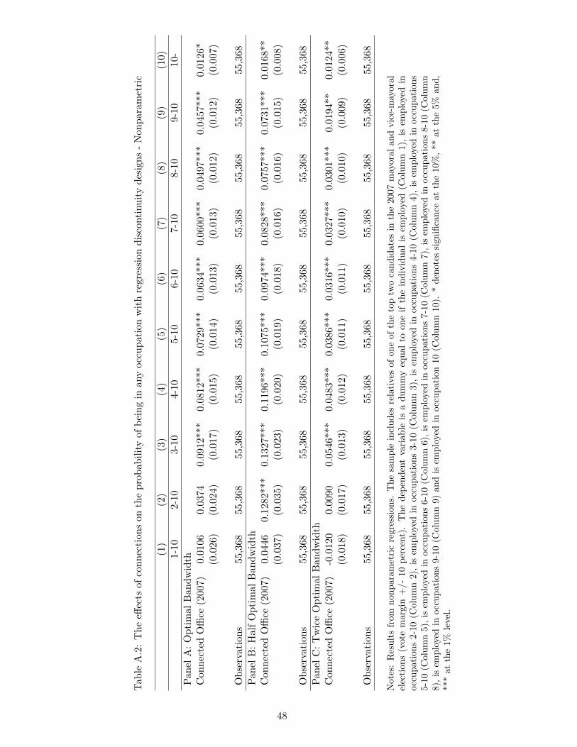
Tab

leA

.2:

The

effec

tsof

conn

ecti

ons

onth

epr

obab

ility

ofbe

ing

inan

yoc

cupa

tion

wit

hre

gres

sion

disc

onti

nuit

yde

sign

s-

Non

para

met

ric

(1)

(2)

(3)

(4)

(5)

(6)

(7)

(8)

(9)

(10)

1-10

2-10

3-10

4-10

5-10

6-10

7-10

8-10

9-10

10-

Pan

elA

:O

ptim

alB

andw

idth

Con

nect

edO

ffice

(200

7)0.

0106

0.03

740.

0912

***

0.08

12**

*0.

0729

***

0.06

34**

*0.

0600

***

0.04

97**

*0.

0457

***

0.01

26*

(0.0

26)

(0.0

24)

(0.0

17)

(0.0

15)

(0.0

14)

(0.0

13)

(0.0

13)

(0.0

12)

(0.0

12)

(0.0

07)

Obs

erva

tion

s55

,368

55,3

6855

,368

55,3

6855

,368

55,3

6855

,368

55,3

6855

,368

55,3

68P

anel

B:

Hal

fO

ptim

alB

andw

idth

Con

nect

edO

ffice

(200

7)0.

0446

0.12

82**

*0.

1327

***

0.11

96**

*0.

1075

***

0.09

74**

*0.

0828

***

0.07

57**

*0.

0731

***

0.01

68**

(0.0

37)

(0.0

35)

(0.0

23)

(0.0

20)

(0.0

19)

(0.0

18)

(0.0

16)

(0.0

16)

(0.0

15)

(0.0

08)

Obs

erva

tion

s55

,368

55,3

6855

,368

55,3

6855

,368

55,3

6855

,368

55,3

6855

,368

55,3

68P

anel

C:

Tw

ice

Opt

imal

Ban

dwid

thC

onne

cted

Offi

ce(2

007)

-0.0

120

0.00

900.

0546

***

0.04

83**

*0.

0386

***

0.03

16**

*0.

0327

***

0.03

01**

*0.

0194

**0.

0124

**(0

.018

)(0

.017

)(0

.013

)(0

.012

)(0

.011

)(0

.011

)(0

.010

)(0

.010

)(0

.009

)(0

.006

)

Obs

erva

tion

s55

,368

55,3

6855

,368

55,3

6855

,368

55,3

6855

,368

55,3

6855

,368

55,3

68

Not

es:

Res

ults

from

nonp

aram

etri

cre

gres

sion

s.T

hesa

mpl

ein

clud

esre

lati

ves

ofon

eof

the

top

two

cand

idat

esin

the

2007

may

oral

and

vice

-may

oral

elec

tion

s(v

ote

mar

gin

+/-

10pe

rcen

t).

The

depe

nden

tva

riab

leis

adu

mm

yeq

ual

toon

eif

the

indi

vidu

alis

empl

oyed

(Col

umn

1),

isem

ploy

edin

occu

pati

ons

2-10

(Col

umn

2),

isem

ploy

edin

occu

pati

ons

3-10

(Col

umn

3),

isem

ploy

edin

occu

pati

ons

4-10

(Col

umn

4),

isem

ploy

edin

occu

pati

ons

5-10

(Col

umn

5),i

sem

ploy

edin

occu

pati

ons

6-10

(Col

umn

6),i

sem

ploy

edin

occu

pati

ons

7-10

(Col

umn

7),i

sem

ploy

edin

occu

pati

ons

8-10

(Col

umn

8),

isem

ploy

edin

occu

pati

ons

9-10

(Col

umn

9)an

dis

empl

oyed

inoc

cupa

tion

10(C

olum

n10

).*

deno

tes

sign

ifica

nce

atth

e10

%,

**at

the

5%an

d,**

*at

the

1%le

vel.

48

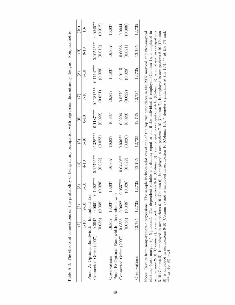
Tab

leA

.3:

The

effec

tsof

conn

ecti

ons

onth

epr

obab

ility

ofbe

ing

inan

yoc

cupa

tion

wit

hre

gres

sion

disc

onti

nuit

yde

sign

s-

Non

para

met

ric

(1)

(2)

(3)

(4)

(5)

(6)

(7)

(8)

(9)

(10)

1-10

2-10

3-10

4-10

5-10

6-10

7-10

8-10

9-10

10-

Pan

elA

:O

ptim

alB

andw

idth

-In

cum

bent

lost

Con

nect

edO

ffice

(200

7)-0

.004

20.

0601

0.14

92**

*0.

1276

***

0.13

28**

*0.

1187

***

0.11

81**

*0.

1114

***

0.10

54**

*0.

0245

**(0

.036

)(0

.038

)(0

.026

)(0

.022

)(0

.023

)(0

.022

)(0

.021

)(0

.020

)(0

.019

)(0

.012

)

Obs

erva

tion

s16

,837

16,8

3716

,837

16,8

3716

,837

16,8

3716

,837

16,8

3716

,837

16,8

37P

anel

B:

Opt

imal

Ban

dwid

th-

Incu

mbe

ntw

onC

onne

cted

Offi

ce(2

007)

0.03

580.

0622

0.05

57**

0.04

40**

0.03

62*

0.02

960.

0279

0.01

150.

0068

0.00

44(0

.036

)(0

.048

)(0

.026

)(0

.022

)(0

.020

)(0

.020

)(0

.022

)(0

.020

)(0

.021

)(0

.008

)

Obs

erva

tion

s12

,735

12,7

3512

,735

12,7

3512

,735

12,7

3512

,735

12,7

3512

,735

12,7

35

Not

es:

Res

ults

from

nonp

aram

etri

cre

gres

sion

s.T

hesa

mpl

ein

clud

esre

lati

ves

ofon

eof

the

top

two

cand

idat

esin

the

2007

may

oral

and

vice

-may

oral

elec

tion

s(v

ote

mar

gin

+/-

5pe

rcen

t).

The

depe

nden

tva

riab

leis

adu

mm

yeq

ual

toon

eif

the

indi

vidu

alis

empl

oyed

(Col

umn

1),

isem

ploy

edin

occu

pati

ons

2-10

(Col

umn

2),

isem

ploy

edin

occu

pati

ons

3-10

(Col

umn

3),

isem

ploy

edin

occu

pati

ons

4-10

(Col

umn

4),

isem

ploy

edin

occu

pati

ons

5-10

(Col

umn

5),i

sem

ploy

edin

occu

pati

ons

6-10

(Col

umn

6),i

sem

ploy

edin

occu

pati

ons

7-10

(Col

umn

7),i

sem

ploy

edin

occu

pati

ons

8-10

(Col

umn

8),

isem

ploy

edin

occu

pati

ons

9-10

(Col

umn

9)an

dis

empl

oyed

inoc

cupa

tion

10(C

olum

n10

).*

deno

tes

sign

ifica

nce

atth

e10

%,

**at

the

5%an

d,**

*at

the

1%le

vel.

49

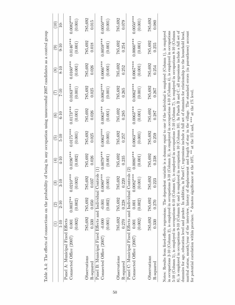
Tab

leA

.4:

The

effec

tsof

conn

ecti

ons

onth

epr

obab

ility

ofbe

ing

inan

yoc

cupa

tion

usin

gun

succ

essf

ul20

07ca

ndid

ates

asa

cont

rolg

roup

(1)

(2)

(3)

(4)

(5)

(6)

(7)

(8)

(9)

(10)

1-10

2-10

3-10

4-10

5-10

6-10

7-10

8-10

9-10

10-

Pan

elA

:M

unic

ipal

Fix

edE

ffect

sC

onne

cted

Offi

ce(2

007)

0.00

10.

0037

**0.

0210

***

0.01

96**

*0.

0175

***

0.01

73**

*0.

0163

***

0.01

60**

*0.

0146

***

0.00

82**

*(0

.002

)(0

.002

)(0

.002

)(0

.002

)(0

.001

)(0

.001

)(0

.001

)(0

.001

)(0

.001

)(0

.001

)

Obs

erva

tion

s78

5,69

278

5,69

278

5,69

278

5,69

278

5,69

278

5,69

278

5,69

278

5,69

278

5,69

278

5,69

2R

-squ

ared

0.33

00.

050

0.03

70.

026

0.02

50.

026

0.02

50.

026

0.01

80.

015

Pan

elB

:M

unic

ipal

Fix

edE

ffect

san

dIn

divi

dual

Con

trol

s(1

)C

onne

cted

Offi

ce(2

007)

-0.0

00-0

.001

0.00

80**

*0.

0079

***

0.00

63**

*0.

0063

***

0.00

62**

*0.

0066

***

0.00

59**

*0.

0050

***

(0.0

01)

(0.0

02)

(0.0

01)

(0.0

01)

(0.0

01)

(0.0

01)

(0.0

01)

(0.0

01)

(0.0

01)

(0.0

01)

Obs

erva

tion

s78

5,69

278

5,69

278

5,69

278

5,69

278

5,69

278

5,69

278

5,69

278

5,69

278

5,69

278

5,69

2R

-squ

ared

0.27

00.

228

0.22

00.

235

0.25

70.

285

0.26

50.

252

0.25

40.

079

Pan

elC

:M

unic

ipal

Fix

edE

ffect

san

dIn

divi

dual

Con

trol

s(2

)C

onne

cted

Offi

ce(2

007)

0.00

10.

001

0.00

82**

*0.

0080

***

0.00

63**

*0.

0063

***

0.00

62**

*0.

0067

***

0.00

60**

*0.

0050

***

(0.0

02)

(0.0

02)

(0.0

01)

(0.0

01)

(0.0

01)

(0.0

01)

(0.0

01)

(0.0

01)

(0.0

01)

(0.0

01)

Obs

erva

tion

s78

5,69

278

5,69

278

5,69

278

5,69

278

5,69

278

5,69

278

5,69

278

5,69

278

5,69

278

5,69

2R

-squ

ared

0.33

00.

270

0.22

30.

238

0.25

90.

287

0.26

70.

254

0.25

50.

080

Not

es:

Res

ults

from

fixed

-effe

cts

regr

essi

ons.

The

depe

nden

tva

riab

leis

adu

mm

yeq

ual

toon

eif

the

indi

vidu

alis

empl

oyed

(Col

umn

1),

isem

ploy

edin

occu

pati

ons

2-10

(Col

umn

2),i

sem

ploy

edin

occu

pati

ons

3-10

(Col

umn

3),i

sem

ploy

edin

occu

pati

ons

4-10

(Col

umn

4),i

sem

ploy

edin

occu

pati

ons

5-10

(Col

umn

5),i

sem

ploy

edin

occu

pati

ons

6-10

(Col

umn

6),i

sem

ploy

edin

occu

pati

ons

7-10

(Col

umn

7),i

sem

ploy

edin

occu

pati

ons

8-10

(Col

umn

8),i

sem

ploy

edin

occu

pati

ons

9-10

(Col

umn

9)an

dis

empl

oyed

inoc

cupa

tion

10(C

olum

n10

).In

Pan

els

Ban

dC

,all

regr

essi

ons

incl

ude

afu

llse

tof

dum

mie

sfo

rag

e,ed

ucat

ion

leve

land

gend

er.

Inad

diti

on,i

nP

anel

C,r

egre

ssio

nsin

clud

ea

full

set

ofdu

mm

ies

for

rela

tion

ship

toth

eho

useh

old

head

,m

arit

alst

atus

,m

onth

/yea

rof

the

inte

rvie

w,

hist

ory

ofdi

spla

cem

ent

and

leng

thof

stay

inth

evi

llage

.T

hest

anda

rder

rors

(in

pare

nthe

ses)

acco

unt

for

pote

ntia

lco

rrel

atio

nw

ithi

npr

ovin

ce.

*de

note

ssi

gnifi

canc

eat

the

10%

,**

atth

e5%

and,

***

atth

e1%

leve

l.

50

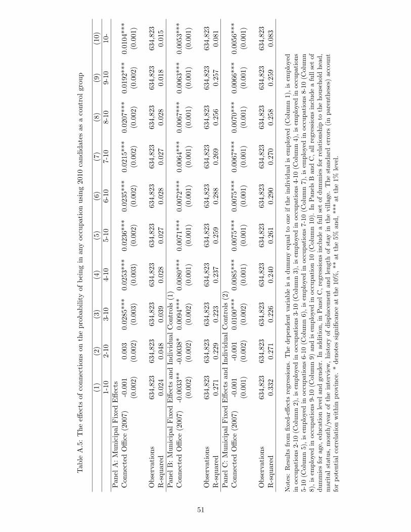
Tab

leA

.5:

The

effec

tsof

conn

ecti

ons

onth

epr

obab

ility

ofbe

ing

inan

yoc

cupa

tion

usin

g20

10ca

ndid

ates

asa

cont

rol

grou

p

(1)

(2)

(3)

(4)

(5)

(6)

(7)

(8)

(9)

(10)

1-10

2-10

3-10

4-10

5-10

6-10

7-10

8-10

9-10

10-

Pan

elA

:M

unic

ipal

Fix

edE

ffect

sC

onne

cted

Offi

ce(2

007)

-0.0

010.

003

0.02

85**

*0.

0253

***

0.02

36**

*0.

0235

***

0.02

15**

*0.

0207

***

0.01

92**

*0.

0104

***

(0.0

02)

(0.0

02)

(0.0

03)

(0.0

03)

(0.0

02)

(0.0

02)

(0.0

02)

(0.0

02)

(0.0

02)

(0.0

01)

Obs

erva

tion

s63

4,82

363

4,82

363

4,82

363

4,82

363

4,82

363

4,82

363

4,82

363

4,82

363

4,82

363

4,82

3R

-squ

ared

0.02

40.

048

0.03

90.

028

0.02

70.

028

0.02

70.

028

0.01

80.

015

Pan

elB

:M

unic

ipal

Fix

edE

ffect

san

dIn

divi

dual

Con

trol

s(1

)C

onne

cted

Offi

ce(2

007)

-0.0

033*

*-0

.003

8*0.

0094

***

0.00

80**

*0.

0071

***

0.00

72**

*0.

0064

***

0.00

67**

*0.

0063

***

0.00

53**

*(0

.002

)(0

.002

)(0

.002

)(0

.001

)(0

.001

)(0

.001

)(0

.001

)(0

.001

)(0

.001

)(0

.001

)

Obs

erva

tion

s63

4,82

363

4,82

363

4,82

363

4,82

363

4,82

363

4,82

363

4,82

363

4,82

363

4,82

363

4,82

3R

-squ

ared

0.27

10.

229

0.22

30.

237

0.25

90.

288

0.26

90.

256

0.25

70.

081

Pan

elC

:M

unic

ipal

Fix

edE

ffect

san

dIn

divi

dual

Con

trol

s(2

)C

onne

cted

Offi

ce(2

007)

-0.0

01-0

.001

0.01

00**

*0.

0085

***

0.00

75**

*0.

0075

***

0.00

67**

*0.

0070

***

0.00

66**

*0.

0056

***

(0.0

01)

(0.0

02)

(0.0

02)

(0.0

01)

(0.0

01)

(0.0

01)

(0.0

01)

(0.0

01)

(0.0

01)

(0.0

01)

Obs

erva

tion

s63

4,82

363

4,82

363

4,82

363

4,82

363

4,82

363

4,82

363

4,82

363

4,82

363

4,82

363

4,82

3R

-squ

ared

0.33

20.

271

0.22

60.

240

0.26

10.

290

0.27

00.

258

0.25

90.

083

Not

es:

Res

ults

from

fixed

-effe

cts

regr

essi

ons.

The

depe

nden

tva

riab

leis

adu

mm

yeq

ual

toon

eif

the

indi

vidu

alis

empl

oyed

(Col

umn

1),

isem

ploy

edin

occu

pati

ons

2-10

(Col

umn

2),i

sem

ploy

edin

occu

pati

ons

3-10

(Col

umn

3),i

sem

ploy

edin

occu

pati

ons

4-10

(Col

umn

4),i

sem

ploy

edin

occu

pati

ons

5-10

(Col

umn

5),i

sem

ploy

edin

occu

pati

ons

6-10

(Col

umn

6),i

sem

ploy

edin

occu

pati

ons

7-10

(Col

umn

7),i

sem

ploy

edin

occu

pati

ons

8-10

(Col

umn

8),i

sem

ploy

edin

occu

pati

ons

9-10

(Col

umn

9)an

dis

empl

oyed

inoc

cupa

tion

10(C

olum

n10

).In

Pan

els

Ban

dC

,all

regr

essi

ons

incl

ude

afu

llse

tof

dum

mie

sfo

rag

e,ed

ucat

ion

leve

land

gend

er.

Inad

diti

on,i

nP

anel

C,r

egre

ssio

nsin

clud

ea

full

set

ofdu

mm

ies

for

rela

tion

ship

toth

eho

useh

old

head

,m

arit

alst

atus

,m

onth

/yea

rof

the

inte

rvie

w,

hist

ory

ofdi

spla

cem

ent

and

leng

thof

stay

inth

evi

llage

.T

hest

anda

rder

rors

(in

pare

nthe

ses)

acco

unt

for

pote

ntia

lco

rrel

atio

nw

ithi

npr

ovin

ce.

*de

note

ssi

gnifi

canc

eat

the

10%

,**

atth

e5%

and,

***

atth

e1%

leve

l.

51

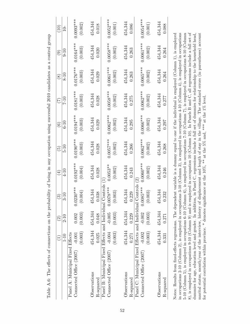
Tab

leA

.6:

The

effec

tsof

conn

ecti

ons

onth

epr

obab

ility

ofbe

ing

inan

yoc

cupa

tion

usin

gsu

cces

sful

2010

cand

idat

esas

aco

ntro

lgr

oup

(1)

(2)

(3)

(4)

(5)

(6)

(7)

(8)

(9)

(10)

1-10

2-10

3-10

4-10

5-10

6-10

7-10

8-10

9-10

10-

Pan

elA

:M

unic

ipal

Fix

edE

ffect

sC

onne

cted

Offi

ce(2

007)

-0.0

010.

002

0.02

30**

*0.

0192

***

0.01

90**

*0.

0194

***

0.01

81**

*0.

0176

***

0.01

64**

*0.

0093

***

(0.0

03)

(0.0

03)

(0.0

04)

(0.0

04)

(0.0

03)

(0.0

03)

(0.0

03)

(0.0

03)

(0.0

03)

(0.0

02)

Obs

erva

tion

s45

4,34

445

4,34

445

4,34

445

4,34

445

4,34

445

4,34

445

4,34

445

4,34

445

4,34

445

4,34

4R

-squ

ared

0.02

50.

048

0.03

80.

028

0.02

80.

029

0.02

80.

029

0.02

00.

018

Pan

elB

:M

unic

ipal

Fix

edE

ffect

san

dIn

divi

dual

Con

trol

s(1

)C

onne

cted

Offi

ce(2

007)

-0.0

04-0

.005

0.00

78**

*0.

0053

**0.

0057

***

0.00

62**

*0.

0058

***

0.00

61**

*0.

0058

***

0.00

52**

*(0

.003

)(0

.003

)(0

.003

)(0

.002

)(0

.002

)(0

.002

)(0

.002

)(0

.002

)(0

.002

)(0

.001

)

Obs

erva

tion

s45

4,34

445

4,34

445

4,34

445

4,34

445

4,34

445

4,34

445

4,34

445

4,34

445

4,34

445

4,34

4R

-squ

ared

0.27

10.

229

0.22

90.

243

0.26

60.

295

0.27

50.

263

0.26

30.

086

Pan

elC

:M

unic

ipal

Fix

edE

ffect

san

dIn

divi

dual

Con

trol

s(2

)C

onne

cted

Offi

ce(2

007)

-0.0

02-0

.002

0.00

85**

*0.

0060

***

0.00

62**

*0.

0066

***

0.00

62**

*0.

0065

***

0.00

61**

*0.

0054

***

(0.0

03)

(0.0

03)

(0.0

03)

(0.0

02)

(0.0

02)

(0.0

02)

(0.0

02)

(0.0

02)

(0.0

02)

(0.0

01)

Obs

erva

tion

s45

4,34

445

4,34

445

4,34

445

4,34

445

4,34

445

4,34

445

4,34

445

4,34

445

4,34

445

4,34

4R

-squ

ared

0.33

10.

271

0.23

20.

246

0.26

80.

297

0.27

70.

264

0.26

40.

088

Not

es:

Res

ults

from

fixed

-effe

cts

regr

essi

ons.

The

depe

nden

tva

riab

leis

adu

mm

yeq

ual

toon

eif

the

indi

vidu

alis

empl

oyed

(Col

umn

1),

isem

ploy

edin

occu

pati

ons

2-10

(Col

umn

2),i

sem

ploy

edin

occu

pati

ons

3-10

(Col

umn

3),i

sem

ploy

edin

occu

pati

ons

4-10

(Col

umn

4),i

sem

ploy

edin

occu

pati

ons

5-10

(Col

umn

5),i

sem

ploy

edin

occu

pati

ons

6-10

(Col

umn

6),i

sem

ploy

edin

occu

pati

ons

7-10

(Col

umn

7),i

sem

ploy

edin

occu

pati

ons

8-10

(Col

umn

8),i

sem

ploy

edin

occu

pati

ons

9-10

(Col

umn

9)an

dis

empl

oyed

inoc

cupa

tion

10(C

olum

n10

).In

Pan

els

Ban

dC

,all

regr

essi

ons

incl

ude

afu

llse

tof

dum

mie

sfo

rag

e,ed

ucat

ion

leve

land

gend

er.

Inad

diti

on,i

nP

anel

C,r

egre

ssio

nsin

clud

ea

full

set

ofdu

mm

ies

for

rela

tion

ship

toth

eho

useh

old

head

,m

arit

alst

atus

,m

onth

/yea

rof

the

inte

rvie

w,

hist

ory

ofdi

spla

cem

ent

and

leng

thof

stay

inth

evi

llage

.T

hest

anda

rder

rors

(in

pare

nthe

ses)

acco

unt

for

pote

ntia

lco

rrel

atio

nw

ithi

npr

ovin

ce.

*de

note

ssi

gnifi

canc

eat

the

10%

,**

atth

e5%

and,

***

atth

e1%

leve

l.

52

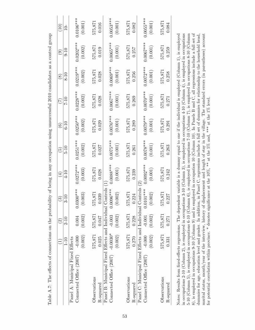
Tab

leA

.7:

The

effec

tsof

conn

ecti

ons

onth

epr

obab

ility

ofbe

ing

inan

yoc

cupa

tion

usin

gun

succ

essf

ul20

10ca

ndid

ates

asa

cont

rolg

roup

(1)

(2)

(3)

(4)

(5)

(6)

(7)

(8)

(9)

(10)

1-10

2-10

3-10

4-10

5-10

6-10

7-10

8-10

9-10

10-

Pan

elA

:M

unic

ipal

Fix

edE

ffect

sC

onne

cted

Offi

ce(2

007)

-0.0

000.

004

0.03

00**

*0.

0272

***

0.02

51**

*0.

0250

***

0.02

28**

*0.

0219

***

0.02

02**

*0.

0106

***

(0.0

02)

(0.0

02)

(0.0

03)

(0.0

03)

(0.0

02)

(0.0

02)

(0.0

02)

(0.0

02)

(0.0

02)

(0.0

01)

Obs

erva

tion

s57

5,87

157

5,87

157

5,87

157

5,87

157

5,87

157

5,87

157

5,87

157

5,87

157

5,87

157

5,87

1R

-squ

ared

0.02

50.

047

0.03

90.

028

0.02

70.

029

0.02

80.

028

0.01

90.

016

Pan

elB

:M

unic

ipal

Fix

edE

ffect

san

dIn

divi

dual

Con

trol

s(1

)C

onne

cted

Offi

ce(2

007)

-0.0

030*

-0.0

030.

0096

***

0.00

88**

*0.

0075

***

0.00

76**

*0.

0067

***

0.00

69**

*0.

0065

***

0.00

53**

*(0

.002

)(0

.002

)(0

.002

)(0

.001

)(0

.001

)(0

.001

)(0

.001

)(0

.001

)(0

.001

)(0

.001

)

Obs

erva

tion

s57

5,87

157

5,87

157

5,87

157

5,87

157

5,87

157

5,87

157

5,87

157

5,87

157

5,87

157

5,87

1R

-squ

ared

0.27

00.

228

0.22

40.

239

0.26

10.

289

0.26

90.

256

0.25

70.

082

Pan

elC

:M

unic

ipal

Fix

edE

ffect

san

dIn

divi

dual

Con

trol

s(2

)C

onne

cted

Offi

ce(2

007)

-0.0

00-0

.001

0.01

01**

*0.

0092

***

0.00

78**

*0.

0079

***

0.00

70**

*0.

0072

***

0.00

67**

*0.

0055

***

(0.0

02)

(0.0

02)

(0.0

02)

(0.0

01)

(0.0

01)

(0.0

01)

(0.0

01)

(0.0

01)

(0.0

01)

(0.0

01)

Obs

erva

tion

s57

5,87

157

5,87

157

5,87

157

5,87

157

5,87

157

5,87

157

5,87

157

5,87

157

5,87

157

5,87

1R

-squ

ared

0.33

10.

271

0.22

70.

242

0.26

30.

291

0.27

10.

258

0.25

90.

084

Not

es:

Res

ults

from

fixed

-effe

cts

regr

essi

ons.

The

depe

nden

tva

riab

leis

adu

mm

yeq

ual

toon

eif

the

indi

vidu

alis

empl

oyed

(Col

umn

1),

isem

ploy

edin

occu

pati

ons

2-10

(Col

umn

2),i

sem

ploy

edin

occu

pati

ons

3-10

(Col

umn

3),i

sem

ploy

edin

occu

pati

ons

4-10

(Col

umn

4),i

sem

ploy

edin

occu

pati

ons

5-10

(Col

umn

5),i

sem

ploy

edin

occu

pati

ons

6-10

(Col

umn

6),i

sem

ploy

edin

occu

pati

ons

7-10

(Col

umn

7),i

sem

ploy

edin

occu

pati

ons

8-10

(Col

umn

8),i

sem

ploy

edin

occu

pati

ons

9-10

(Col

umn

9)an

dis

empl

oyed

inoc

cupa

tion

10(C

olum

n10

).In

Pan

els

Ban

dC

,all

regr

essi

ons

incl

ude

afu

llse

tof

dum

mie

sfo

rag

e,ed

ucat

ion

leve

land

gend

er.

Inad

diti

on,i

nP

anel

C,r

egre

ssio

nsin

clud

ea

full

set

ofdu

mm

ies

for

rela

tion

ship

toth

eho

useh

old

head

,m

arit

alst

atus

,m

onth

/yea

rof

the

inte

rvie

w,

hist

ory

ofdi

spla

cem

ent

and

leng

thof

stay

inth

evi

llage

.T

hest

anda

rder

rors

(in

pare

nthe

ses)

acco

unt

for

pote

ntia

lco

rrel

atio

nw

ithi

npr

ovin

ce.

*de

note

ssi

gnifi

canc

eat

the

10%

,**

atth

e5%

and,

***

atth

e1%

leve

l.

53

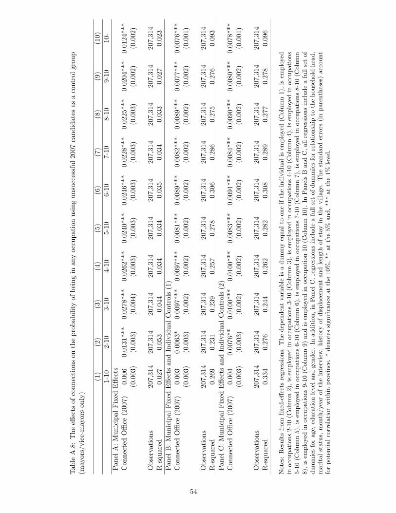
Tab

leA

.8:

The

effec

tsof

conn

ecti

ons

onth

epr

obab

ility

ofbe

ing

inan

yoc

cupa

tion

usin

gun

succ

essf

ul20

07ca

ndid

ates

asa

cont

rolg

roup

(may

ors/

vice

-may

ors

only

)

(1)

(2)

(3)

(4)

(5)

(6)

(7)

(8)

(9)

(10)

1-10

2-10

3-10

4-10

5-10

6-10

7-10

8-10

9-10

10-

Pan

elA

:M

unic

ipal

Fix

edE

ffect

sC

onne

cted

Offi

ce(2

007)

0.00

60.

0131

***

0.02

78**

*0.

0262

***

0.02

40**

*0.

0246

***

0.02

28**

*0.

0225

***

0.02

04**

*0.

0124

***

(0.0

03)

(0.0

03)

(0.0

04)

(0.0

03)

(0.0

03)

(0.0

03)

(0.0

03)

(0.0

03)

(0.0

02)

(0.0

02)

Obs

erva

tion

s20

7,31

420

7,31

420

7,31

420

7,31

420

7,31

420

7,31

420

7,31

420

7,31

420

7,31

420

7,31

4R

-squ

ared

0.02

70.

053

0.04

40.

034

0.03

40.

035

0.03

40.

033

0.02

70.

023

Pan

elB

:M

unic

ipal

Fix

edE

ffect

san

dIn

divi

dual

Con

trol

s(1

)C

onne

cted

Offi

ce(2

007)

0.00

30.

0063

*0.

0097

***

0.00

97**

*0.

0081

***

0.00

89**

*0.

0082

***

0.00

89**

*0.

0077

***

0.00

76**

*(0

.003

)(0

.003

)(0

.002

)(0

.002

)(0

.002

)(0

.002

)(0

.002

)(0

.002

)(0

.002

)(0

.001

)

Obs

erva

tion

s20

7,31

420

7,31

420

7,31

420

7,31

420

7,31

420

7,31

420

7,31

420

7,31

420

7,31

420

7,31

4R

-squ

ared

0.26

90.

231

0.23

90.

257

0.27

80.

306

0.28

60.

275

0.27

60.

093

Pan

elC

:M

unic

ipal

Fix

edE

ffect

san

dIn

divi

dual

Con

trol

s(2

)C

onne

cted

Offi

ce(2

007)

0.00

40.

0076

**0.

0100

***

0.01

00**

*0.

0083

***

0.00

91**

*0.

0084

***

0.00

90**

*0.

0080

***

0.00

78**

*(0

.003

)(0

.003

)(0

.002

)(0

.002

)(0

.002

)(0

.002

)(0

.002

)(0

.002

)(0

.002

)(0

.001

)

Obs

erva

tion

s20

7,31

420

7,31

420

7,31

420

7,31

420

7,31

420

7,31

420

7,31

420

7,31

420

7,31

420

7,31

4R

-squ

ared

0.33

40.

276

0.24

40.

262

0.28

20.

308

0.28

90.

277

0.27

80.

096

Not

es:

Res

ults

from

fixed

-effe

cts

regr

essi

ons.

The

depe

nden

tva

riab

leis

adu

mm

yeq

ual

toon

eif

the

indi

vidu

alis

empl

oyed

(Col

umn

1),

isem

ploy

edin

occu

pati

ons

2-10

(Col

umn

2),i

sem

ploy

edin

occu

pati

ons

3-10

(Col

umn

3),i

sem

ploy

edin

occu

pati

ons

4-10

(Col

umn

4),i

sem

ploy

edin

occu

pati

ons

5-10

(Col

umn

5),i

sem

ploy

edin

occu

pati

ons

6-10

(Col

umn

6),i

sem

ploy

edin

occu

pati

ons

7-10

(Col

umn

7),i

sem

ploy

edin

occu

pati

ons

8-10

(Col

umn

8),i

sem

ploy

edin

occu

pati

ons

9-10

(Col

umn

9)an

dis

empl

oyed

inoc

cupa

tion

10(C

olum

n10

).In

Pan

els

Ban

dC

,all

regr

essi

ons

incl

ude

afu

llse

tof

dum

mie

sfo

rag

e,ed

ucat

ion

leve

land

gend

er.

Inad

diti

on,i

nP

anel

C,r

egre

ssio

nsin

clud

ea

full

set

ofdu

mm

ies

for

rela

tion

ship

toth

eho

useh

old

head

,m

arit

alst

atus

,m

onth

/yea

rof

the

inte

rvie

w,

hist

ory

ofdi

spla

cem

ent

and

leng

thof

stay

inth

evi

llage

.T

hest

anda

rder

rors

(in

pare

nthe

ses)

acco

unt

for

pote

ntia

lco

rrel

atio

nw

ithi

npr

ovin

ce.

*de

note

ssi

gnifi

canc

eat

the

10%

,**

atth

e5%

and,

***

atth

e1%

leve

l.

54

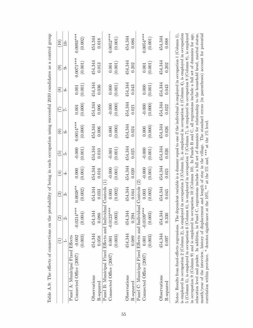
Tab

leA

.9:

The

effec

tsof

conn

ecti

ons

onth

epr

obab

ility

ofbe

ing

inea

choc

cupa

tion

usin

gsu

cces

sful

2010

cand

idat

esas

aco

ntro

lgr

oup

(1)

(2)

(3)

(4)

(5)

(6)

(7)

(8)

(9)

(10)

1-2-

3-4-

5-6-

7-8-

9-10

-P

anel

A:

Mun

icip

alF

ixed

Effe

cts

Con

nect

edO

ffice

(200

7)-0

.002

-0.0

214*

**0.

0038

**0.

000

-0.0

000.

0014

***

0.00

10.

001

0.00

71**

*0.

0093

***

(0.0

03)

(0.0

04)

(0.0

02)

(0.0

01)

(0.0

01)

(0.0

00)

(0.0

00)

(0.0

01)

(0.0

01)

(0.0

02)

Obs

erva

tion

s45

4,34

445

4,34

445

4,34

445

4,34

445

4,34

445

4,34

445

4,34

445

4,34

445

4,34

445

4,34

4R

-squ

ared

0.05

80.

080

0.03

30.

016

0.01

00.

006

0.00

60.

036

0.01

30.

018

Pan

elB

:M

unic

ipal

Fix

edE

ffect

san

dIn

divi

dual

Con

trol

s(1

)C

onne

cted

Offi

ce(2

007)

0.00

1-0

.012

3***

0.00

3-0

.000

-0.0

010.

000

-0.0

000.

000

0.00

10.

0052

***

(0.0

03)

(0.0

03)

(0.0

02)

(0.0

01)

(0.0

01)

(0.0

00)

(0.0

00)

(0.0

01)

(0.0

01)

(0.0

01)

Obs

erva

tion

s45

4,34

445

4,34

445

4,34

445

4,34

445

4,34

445

4,34

445

4,34

445

4,34

445

4,34

445

4,34

4R

-squ

ared

0.08

90.

294

0.04

40.

020

0.02

50.

024

0.02

10.

043

0.20

20.

086

Pan

elC

:M

unic

ipal

Fix

edE

ffect

san

dIn

divi

dual

Con

trol

s(2

)C

onne

cted

Offi

ce(2

007)

0.00

1-0

.010

9***

0.00

3-0

.000

-0.0

000.

000

-0.0

000.

000

0.00

10.

0054

***

(0.0

03)

(0.0

03)

(0.0

02)

(0.0

01)

(0.0

01)

(0.0

00)

(0.0

00)

(0.0

01)

(0.0

01)

(0.0

01)

Obs

erva

tion

s45

4,34

445

4,34

445

4,34

445

4,34

445

4,34

445

4,34

445

4,34

445

4,34

445

4,34

445

4,34

4R

-squ

ared

0.09

70.

330

0.04

50.

021

0.02

60.

026

0.02

20.

043

0.20

20.

088

Not

es:

Res

ults

from

fixed

-effe

cts

regr

essi

ons.

The

depe

nden

tva

riab

leis

adu

mm

yeq

ualt

oon

eif

the

indi

vidu

alis

empl

oyed

inoc

cupa

tion

1(C

olum

n1)

,is

empl

oyed

inoc

cupa

tion

2(C

olum

n2)

,is

empl

oyed

inoc

cupa

tion

3(C

olum

n3)

,is

empl

oyed

inoc

cupa

tion

4(C

olum

n4)

,is

empl

oyed

inoc

cupa

tion

5(C

olum

n5)

,is

empl

oyed

inoc

cupa

tion

6(C

olum

n6)

,is

empl

oyed

inoc

cupa

tion

7(C

olum

n7)

,is

empl

oyed

inoc

cupa

tion

8(C

olum

n8)

,is

empl

oyed

inoc

cupa

tion

9(C

olum

n9)

and

isem

ploy

edin

occu

pati

on10

(Col

umn

10).

InP

anel

sB

and

C,

all

regr

essi

ons

incl

ude

afu

llse

tof

dum

mie

sfo

rag

e,ed

ucat

ion

leve

lan

dge

nder

.In

addi

tion

,in

Pan

elC

,re

gres

sion

sin

clud

ea

full

set

ofdu

mm

ies

for

rela

tion

ship

toth

eho

useh

old

head

,m

arit

alst

atus

,m

onth

/yea

rof

the

inte

rvie

w,

hist

ory

ofdi

spla

cem

ent

and

leng

thof

stay

inth

evi

llage

.T

hest

anda

rder

rors

(in

pare

nthe

ses)

acco

unt

for

pote

ntia

lco

rrel

atio

nw

ithi

npr

ovin

ce.

*de

note

ssi

gnifi

canc

eat

the

10%

,**

atth

e5%

and,

***

atth

e1%

leve

l.

55

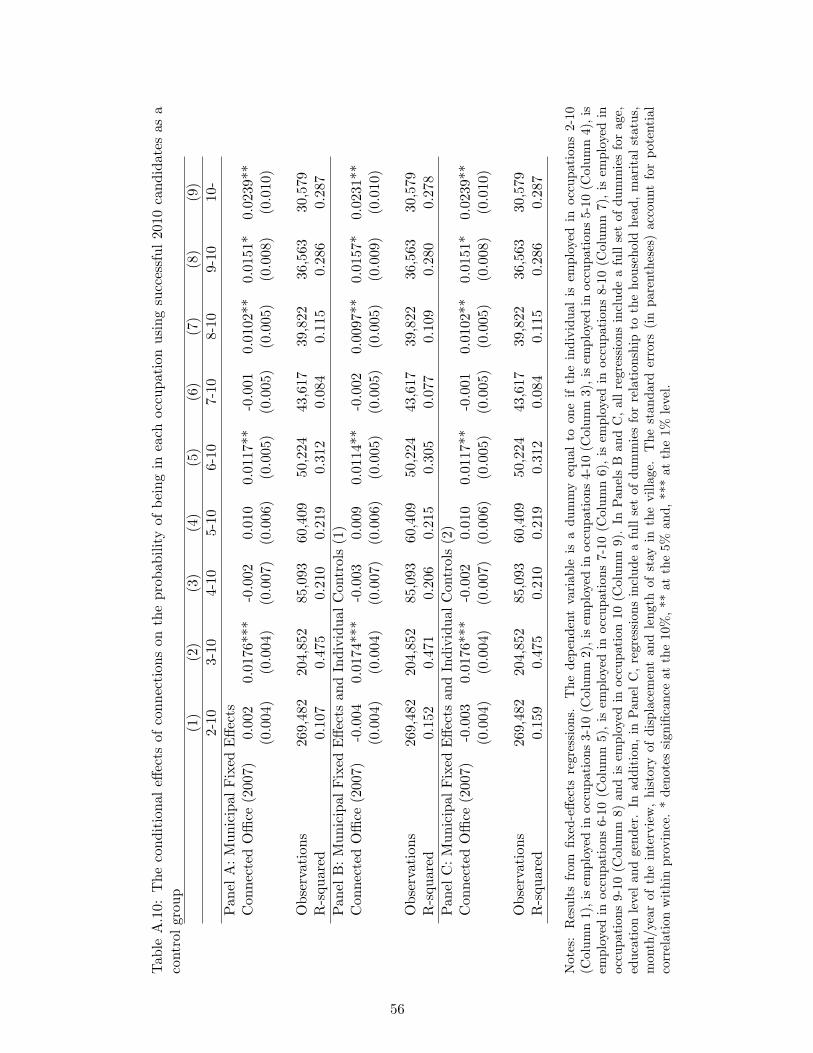
Tab

leA

.10:

The

cond

itio

nal

effec

tsof

conn

ecti

ons

onth

epr

obab

ility

ofbe

ing

inea

choc

cupa

tion

usin

gsu

cces

sful

2010

cand

idat

esas

aco

ntro

lgr

oup

(1)

(2)

(3)

(4)

(5)

(6)

(7)

(8)

(9)

2-10

3-10

4-10

5-10

6-10

7-10

8-10

9-10

10-

Pan

elA

:M

unic

ipal

Fix

edE

ffect

sC

onne

cted

Offi

ce(2

007)

0.00

20.

0176

***

-0.0

020.

010

0.01

17**

-0.0

010.

0102

**0.

0151

*0.

0239

**(0

.004

)(0

.004

)(0

.007

)(0

.006

)(0

.005

)(0

.005

)(0

.005

)(0

.008

)(0

.010

)

Obs

erva

tion

s26

9,48

220

4,85

285

,093

60,4

0950

,224

43,6

1739

,822

36,5

6330

,579

R-s

quar

ed0.

107

0.47

50.

210

0.21

90.

312

0.08

40.

115

0.28

60.

287

Pan

elB

:M

unic

ipal

Fix

edE

ffect

san

dIn

divi

dual

Con

trol

s(1

)C

onne

cted

Offi

ce(2

007)

-0.0

040.

0174

***

-0.0

030.

009

0.01

14**

-0.0

020.

0097

**0.

0157

*0.

0231

**(0

.004

)(0

.004

)(0

.007

)(0

.006

)(0

.005

)(0

.005

)(0

.005

)(0

.009

)(0

.010

)

Obs

erva

tion

s26

9,48

220

4,85

285

,093

60,4

0950

,224

43,6

1739

,822

36,5

6330

,579

R-s

quar

ed0.

152

0.47

10.

206

0.21

50.

305

0.07

70.

109

0.28

00.

278

Pan

elC

:M

unic

ipal

Fix

edE

ffect

san

dIn

divi

dual

Con

trol

s(2

)C

onne

cted

Offi

ce(2

007)

-0.0

030.

0176

***

-0.0

020.

010

0.01

17**

-0.0

010.

0102

**0.

0151

*0.

0239

**(0

.004

)(0

.004

)(0

.007

)(0

.006

)(0

.005

)(0

.005

)(0

.005

)(0

.008

)(0

.010

)

Obs

erva

tion

s26

9,48

220

4,85

285

,093

60,4

0950

,224

43,6

1739

,822

36,5

6330

,579

R-s

quar

ed0.

159

0.47

50.

210

0.21

90.

312

0.08

40.

115

0.28

60.

287

Not

es:

Res

ults

from

fixed

-effe

cts

regr

essi

ons.

The

depe

nden

tva

riab

leis

adu

mm

yeq

ual

toon

eif

the

indi

vidu

alis

empl

oyed

inoc

cupa

tion

s2-

10(C

olum

n1)

,is

empl

oyed

inoc

cupa

tion

s3-

10(C

olum

n2)

,is

empl

oyed

inoc

cupa

tion

s4-

10(C

olum

n3)

,is

empl

oyed

inoc

cupa

tion

s5-

10(C

olum

n4)

,is

empl

oyed

inoc

cupa

tion

s6-

10(C

olum

n5)

,is

empl

oyed

inoc

cupa

tion

s7-

10(C

olum

n6)

,is

empl

oyed

inoc

cupa

tion

s8-

10(C

olum

n7)

,is

empl

oyed

inoc

cupa

tion

s9-

10(C

olum

n8)

and

isem

ploy

edin

occu

pati

on10

(Col

umn

9).

InP

anel

sB

and

C,

all

regr

essi

ons

incl

ude

afu

llse

tof

dum

mie

sfo

rag

e,ed

ucat

ion

leve

lan

dge

nder

.In

addi

tion

,in

Pan

elC

,re

gres

sion

sin

clud

ea

full

set

ofdu

mm

ies

for

rela

tion

ship

toth

eho

useh

old

head

,m

arit

alst

atus

,m

onth

/yea

rof

the

inte

rvie

w,

hist

ory

ofdi

spla

cem

ent

and

leng

thof

stay

inth

evi

llage

.T

hest

anda

rder

rors

(in

pare

nthe

ses)

acco

unt

for

pote

ntia

lco

rrel

atio

nw

ithi

npr

ovin

ce.

*de

note

ssi

gnifi

canc

eat

the

10%

,**

atth

e5%

and,

***

atth

e1%

leve

l.

56

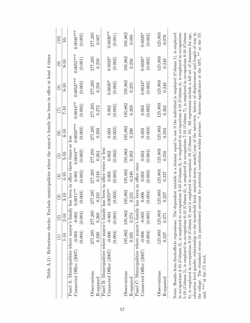
Tab

leA

.11:

Rob

ustn

ess

chec

ks:

Exc

lude

mun

icip

alit

ies

whe

reth

em

ayor

’sfa

mily

has

been

inoffi

ceat

leas

t4

tim

es

(1)

(2)

(3)

(4)

(5)

(6)

(7)

(8)

(9)

(10)

1-10

2-10

3-10

4-10

5-10

6-10

7-10

8-10

9-10

10-

Pan

elA

:M

unic

ipal

itie

sw

here

may

or’s

fam

ilyha

sbe

enin

office

thre

eti

mes

orle

ssC

onne

cted

Offi

ce(2

007)

-0.0

03-0

.002

0.00

71**

0.00

30.

0044

**0.

0050

***

0.00

44**

0.00

53**

*0.

0055

***

0.00

46**

*(0

.004

)(0

.004

)(0

.003

)(0

.002

)(0

.002

)(0

.002

)(0

.002

)(0

.002

)(0

.001

)(0

.002

)

Obs

erva

tion

s27

7,28

527

7,28

527

7,28

527

7,28

527

7,28

527

7,28

527

7,28

527

7,28

527

7,28

527

7,28

5R

-squ

ared

0.33

00.

268

0.23

10.

243

0.26

40.

293

0.27

20.

258

0.25

90.

087

Pan

elB

:M

unic

ipal

itie

sw

here

may

or’s

fam

ilyha

sbe

enin

office

twic

eor

less

Con

nect

edO

ffice

(200

7)-0

.006

-0.0

040.

0070

**0.

003

0.00

20.

003

0.00

20.

0030

*0.

0028

*0.

0036

**(0

.004

)(0

.004

)(0

.003

)(0

.003

)(0

.002

)(0

.002

)(0

.002

)(0

.002

)(0

.002

)(0

.001

)

Obs

erva

tion

s19

5,86

219

5,86

219

5,86

219

5,86

219

5,86

219

5,86

219

5,86

219

5,86

219

5,86

219

5,86

2R

-squ

ared

0.33

50.

274

0.23

10.

240

0.26

20.

290

0.26

90.

255

0.25

60.

088

Pan

elC

:M

unic

ipal

itie

sw

here

may

or’s

fam

ilyha

sbe

enin

office

once

Con

nect

edO

ffice

(200

7)-0

.006

-0.0

030.

006

0.00

30.

003

0.00

30.

003

0.00

44*

0.00

38*

0.00

28*

(0.0

04)

(0.0

05)

(0.0

04)

(0.0

03)

(0.0

04)

(0.0

03)

(0.0

02)

(0.0

02)

(0.0

02)

(0.0

02)

Obs

erva

tion

s12

5,80

312

5,80

312

5,80

312

5,80

312

5,80

312

5,80

312

5,80

312

5,80

312

5,80

312

5,80

3R

-squ

ared

0.33

70.

271

0.22

70.

237

0.25

80.

283

0.26

20.

248

0.24

90.

078

Not

es:

Res

ults

from

fixed

-effe

cts

regr

essi

ons.

The

depe

nden

tva

riab

leis

adu

mm

yeq

ual

toon

eif

the

indi

vidu

alis

empl

oyed

(Col

umn

1),

isem

ploy

edin

occu

pati

ons

2-10

(Col

umn

2),i

sem

ploy

edin

occu

pati

ons

3-10

(Col

umn

3),i

sem

ploy

edin

occu

pati

ons

4-10

(Col

umn

4),i

sem

ploy

edin

occu

pati

ons

5-10

(Col

umn

5),i

sem

ploy

edin

occu

pati

ons

6-10

(Col

umn

6),i

sem

ploy

edin

occu

pati

ons

7-10

(Col

umn

7),i

sem

ploy

edin

occu

pati

ons

8-10

(Col

umn

8),

isem

ploy

edin

occu

pati

ons

9-10

(Col

umn

9)an

dis

empl

oyed

inoc

cupa

tion

10(C

olum

n10

).A

llre

gres

sion

sin

clud

ea

full

set

ofdu

mm

ies

for

age,

educ

atio

nle

vel

gend

er,

rela

tion

ship

toth

eho

useh

old

head

,m

arit

alst

atus

,m

onth

/yea

rof

the

inte

rvie

w,

hist

ory

ofdi

spla

cem

ent

and

leng

thof

stay

inth

evi

llage

.T

hest

anda

rder

rors

(in

pare

nthe

ses)

acco

unt

for

pote

ntia

lco

rrel

atio

nw

ithi

npr

ovin

ce.

*de

note

ssi

gnifi

canc

eat

the

10%

,**

atth

e5%

and,

***

atth

e1%

leve

l.

57

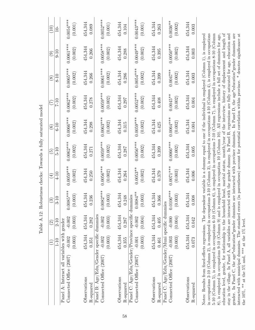
Tab

leA

.12:

Rob

ustn

ess

chec

ks:

Tow

ards

afu

llysa

tura

ted

mod

el

(1)

(2)

(3)

(4)

(5)

(6)

(7)

(8)

(9)

(10)

1-10

2-10

3-10

4-10

5-10

6-10

7-10

8-10

9-10

10-

Pan

elA

:In

tera

ctal

lva

riab

les

wit

hge

nder

Con

nect

edO

ffice

(200

7)-0

.002

-0.0

020.

0085

***

0.00

59**

*0.

0062

***

0.00

66**

*0.

0062

***

0.00

65**

*0.

0061

***

0.00

54**

*(0

.003

)(0

.003

)(0

.003

)(0

.002

)(0

.002

)(0

.002

)(0

.002

)(0

.002

)(0

.002

)(0

.001

)

Obs

erva

tion

s45

4,34

445

4,34

445

4,34

445

4,34

445

4,34

445

4,34

445

4,34

445

4,34

445

4,34

445

4,34

4R

-squ

ared

0.35

10.

282

0.23

60.

250

0.27

10.

298

0.27

80.

266

0.26

60.

089

Pan

elB

:A

ge/E

du/G

ende

rsp

ecifi

cdu

mm

ies

Con

nect

edO

ffice

(200

7)-0

.002

-0.0

020.

0082

***

0.00

56**

*0.

0059

***

0.00

63**

*0.

0059

***

0.00

61**

*0.

0058

***

0.00

52**

*(0

.003

)(0

.003

)(0

.003

)(0

.002

)(0

.002

)(0

.002

)(0

.002

)(0

.002

)(0

.002

)(0

.001

)

Obs

erva

tion

s45

4,34

445

4,34

445

4,34

445

4,34

445

4,34

445

4,34

445

4,34

445

4,34

445

4,34

445

4,34

4R

-squ

ared

0.35

50.

287

0.24

80.

264

0.28

70.

315

0.29

70.

286

0.28

80.

104

Pan

elC

:A

ge/E

du/G

ende

r/P

rovi

nce

spec

ific

dum

mie

sC

onne

cted

Offi

ce(2

007)

-0.0

01-0

.002

0.00

84**

0.00

53**

0.00

56**

*0.

0059

***

0.00

52**

*0.

0054

***

0.00

49**

*0.

0043

***

(0.0

03)

(0.0

04)

(0.0

03)

(0.0

02)

(0.0

02)

(0.0

02)

(0.0

02)

(0.0

02)

(0.0

02)

(0.0

01)

Obs

erva

tion

s45

4,34

445

4,34

445

4,34

445

4,34

445

4,34

445

4,34

445

4,34

445

4,34

445

4,34

445

4,34

4R

-squ

ared

0.46

10.

405

0.36

60.

379

0.39

90.

425

0.40

80.

399

0.39

50.

263

Pan

elC

:A

ge/E

du/G

ende

r/M

uni

spec

ific

dum

mie

sC

onne

cted

Offi

ce(2

007)

-0.0

03-0

.000

0.01

06**

*0.

0071

***

0.00

66**

*0.

0064

***

0.00

45**

0.00

47**

0.00

50**

*0.

0036

**(0

.003

)(0

.004

)(0

.003

)(0

.003

)(0

.002

)(0

.002

)(0

.002

)(0

.002

)(0

.002

)(0

.002

)

Obs

erva

tion

s45

4,34

445

4,34

445

4,34

445

4,34

445

4,34

445

4,34

445

4,34

445

4,34

445

4,34

445

4,34

4R

-squ

ared

0.07

30.

042

0.00

80.

006

0.00

50.

004

0.00

40.

003

0.00

30.

003

Not

es:

Res

ults

from

fixed

-effe

cts

regr

essi

ons.

The

depe

nden

tva

riab

leis

adu

mm

yeq

ual

toon

eif

the

indi

vidu

alis

empl

oyed

(Col

umn

1),

isem

ploy

edin

occu

pati

ons

2-10

(Col

umn

2),i

sem

ploy

edin

occu

pati

ons

3-10

(Col

umn

3),i

sem

ploy

edin

occu

pati

ons

4-10

(Col

umn

4),i

sem

ploy

edin

occu

pati

ons

5-10

(Col

umn

5),i

sem

ploy

edin

occu

pati

ons

6-10

(Col

umn

6),i

sem

ploy

edin

occu

pati

ons

7-10

(Col

umn

7),i

sem

ploy

edin

occu

pati

ons

8-10

(Col

umn

8),

isem

ploy

edin

occu

pati

ons

9-10

(Col

umn

9)an

dis

empl

oyed

inoc

cupa

tion

10(C

olum

n10

).A

llre

gres

sion

sin

clud

ea

full

set

ofdu

mm

ies

for

age,

educ

atio

nle

vel,

gend

er,

for

rela

tion

ship

toth

eho

useh

old

head

,m

arit

alst

atus

,m

onth

/yea

rof

the

inte

rvie

w,

hist

ory

ofdi

spla

cem

ent

and

leng

thof

stay

inth

evi

llage

.In

Pan

elA

,al

lva

riab

les

are

inte

ract

edw

ith

the

gend

erdu

mm

y.In

Pan

elB

,re

gres

sion

sar

efu

llysa

tura

ted

for

age,

educ

atio

nan

dge

nder

.In

Pan

elC

,th

eag

e*ed

ucat

ion*

gend

erdu

mm

ies

are

inte

ract

edw

ith

prov

ince

dum

mie

s.In

Pan

elD

,th

eag

e*ed

ucat

ion*

gend

erdu

mm

ies

are

inte

ract

edw

ith

mun

icip

aldu

mm

ies.

The

stan

dard

erro

rs(i

npa

rent

hese

s)ac

coun

tfo

rpo

tent

ial

corr

elat

ion

wit

hin

prov

ince

.*

deno

tes

sign

ifica

nce

atth

e10

%,

**at

the

5%an

d,**

*at

the

1%le

vel.

58

Tab

leA

.13:

Rob

ustn

ess

chec

ks:

Con

trol

ling

for

Net

wor

kSi

ze

(1)

(2)

(3)

(4)

(5)

(6)

(7)

(8)

(9)

(10)

1-10

2-10

3-10

4-10

5-10

6-10

7-10

8-10

9-10

10-

Pan

elA

:M

unic

ipal

Fix

edE

ffect

sC

onne

cted

Offi

ce(2

007)

-0.0

000.

002

0.02

61**

*0.

0216

***

0.02

15**

*0.

0214

***

0.01

99**

*0.

0191

***

0.01

76**

*0.

0096

***

(0.0

03)

(0.0

03)

(0.0

04)

(0.0

03)

(0.0

03)

(0.0

03)

(0.0

03)

(0.0

03)

(0.0

03)

(0.0

02)

Obs

erva

tion

s45

4,34

445

4,34

445

4,34

445

4,34

445

4,34

445

4,34

445

4,34

445

4,34

445

4,34

445

4,34

4R

-squ

ared

0.02

90.

053

0.04

20.

032

0.03

10.

032

0.03

10.

032

0.02

30.

019

Pan

elB

:M

unic

ipal

Fix

edE

ffect

san

dIn

divi

dual

Con

trol

s(1

)C

onne

cted

Offi

ce(2

007)

-0.0

04-0

.005

0.00

92**

*0.

0063

***

0.00

68**

*0.

0069

***

0.00

64**

*0.

0065

***

0.00

59**

*0.

0050

***

(0.0

03)

(0.0

03)

(0.0

03)

(0.0

02)

(0.0

02)

(0.0

02)

(0.0

02)

(0.0

02)

(0.0

01)

(0.0

01)

Obs

erva

tion

s45

4,34

445

4,34

445

4,34

445

4,34

445

4,34

445

4,34

445

4,34

445

4,34

445

4,34

445

4,34

4R

-squ

ared

0.27

30.

232

0.23

00.

245

0.26

70.

296

0.27

60.

264

0.26

40.

087

Pan

elC

:M

unic

ipal

Fix

edE

ffect

san

dIn

divi

dual

Con

trol

s(2

)C

onne

cted

Offi

ce(2

007)

-0.0

01-0

.002

0.00

97**

*0.

0067

***

0.00

70**

*0.

0071

***

0.00

67**

*0.

0068

***

0.00

62**

*0.

0052

***

(0.0

03)

(0.0

03)

(0.0

03)

(0.0

02)

(0.0

02)

(0.0

02)

(0.0

02)

(0.0

02)

(0.0

01)

(0.0

01)

Obs

erva

tion

s45

4,34

445

4,34

445

4,34

445

4,34

445

4,34

445

4,34

445

4,34

445

4,34

445

4,34

445

4,34

4R

-squ

ared

0.33

20.

273

0.23

30.

247

0.26

90.

298

0.27

80.

265

0.26

50.

089

Not

es:

Res

ults

from

fixed

-effe

cts

regr

essi

ons.

The

depe

nden

tva

riab

leis

adu

mm

yeq

ual

toon

eif

the

indi

vidu

alis

empl

oyed

(Col

umn

1),

isem

ploy

edin

occu

pati

ons

2-10

(Col

umn

2),i

sem

ploy

edin

occu

pati

ons

3-10

(Col

umn

3),i

sem

ploy

edin

occu

pati

ons

4-10

(Col

umn

4),i

sem

ploy

edin

occu

pati

ons

5-10

(Col

umn

5),i

sem

ploy

edin

occu

pati

ons

6-10

(Col

umn

6),i

sem

ploy

edin

occu

pati

ons

7-10

(Col

umn

7),i

sem

ploy

edin

occu

pati

ons

8-10

(Col

umn

8),i

sem

ploy

edin

occu

pati

ons

9-10

(Col

umn

9)an

dis

empl

oyed

inoc

cupa

tion

10(C

olum

n10

).A

llre

gres

sion

sin

clud

ea

full

ofse

tof

dum

mie

sfo

rth

enu

mbe

rof

indi

vidu

als

who

shar

eth

ein

divi

dual

’sm

iddl

ena

me

inth

em

unic

ipal

ity

and

for

the

num

ber

ofin

divi

dual

sw

hosh

are

the

indi

vidu

al’s

mid

dle

nam

ein

the

mun

icip

alit

y.In

Pan

els

Ban

dC

,all

regr

essi

ons

incl

ude

afu

llse

tof

dum

mie

sfo

rag

e,ed

ucat

ion

leve

land

gend

er.

Inad

diti

on,i

nP

anel

C,

regr

essi

ons

incl

ude

afu

llse

tof

dum

mie

sfo

rre

lati

onsh

ipto

the

hous

ehol

dhe

ad,

mar

ital

stat

us,

mon

th/y

ear

ofth

ein

terv

iew

,hi

stor

yof

disp

lace

men

tan

dle

ngth

ofst

ayin

the

villa

ge.

The

stan

dard

erro

rs(i

npa

rent

hese

s)ac

coun

tfo

rpo

tent

ial

corr

elat

ion

wit

hin

prov

ince

.*

deno

tes

sign

ifica

nce

atth

e10

%,

**at

the

5%an

d,**

*at

the

1%le

vel.

59

Tab

leA

.14:

Rob

ustn

ess

chec

ks:

Exc

lude

data

colle

cted

afte

rN

ovem

ber

2009

(1)

(2)

(3)

(4)

(5)

(6)

(7)

(8)

(9)

(10)

1-10

2-10

3-10

4-10

5-10

6-10

7-10

8-10

9-10

10-

Pan

elA

:M

unic

ipal

Fix

edE

ffect

san

dIn

divi

dual

Con

trol

s(2

)C

onne

cted

Offi

ce(2

007)

-0.0

010.

000

0.01

16**

*0.

0079

***

0.00

77**

*0.

0081

***

0.00

75**

*0.

0076

***

0.00

76**

*0.

0065

***

(0.0

03)

(0.0

03)

(0.0

03)

(0.0

03)

(0.0

02)

(0.0

02)

(0.0

02)

(0.0

02)

(0.0

02)

(0.0

02)

Obs

erva

tion

s32

6,65

632

6,65

632

6,65

632

6,65

632

6,65

632

6,65

632

6,65

632

6,65

632

6,65

632

6,65

6R

-squ

ared

0.31

90.

262

0.22

90.

242

0.26

60.

296

0.27

50.

262

0.26

20.

088

Pan

elB

:A

ddIn

tera

ctio

nT

erm

Con

nect

edO

ffice

(200

7)-0

.001

2-0

.000

10.

0116

***

0.00

80**

*0.

0078

***

0.00

81**

*0.

0076

***

0.00

77**

*0.

0076

***

0.00

65**

*(0

.003

)(0

.003

)(0

.003

)(0

.003

)(0

.002

)(0

.002

)(0

.002

)(0

.002

)(0

.002

)(0

.002

)C

onne

cted

Offi

ce(2

007)

X0.

0000

0.00

01-0

.000

3-0

.000

4-0

.000

3-0

.000

2-0

.000

3-0

.000

4-0

.000

3-0

.000

1M

onth

sbe

fore

11/2

009

(0.0

00)

(0.0

01)

(0.0

00)

(0.0

00)

(0.0

00)

(0.0

00)

(0.0

00)

(0.0

00)

(0.0

00)

(0.0

00)

Obs

erva

tion

s32

6,65

632

6,65

632

6,65

632

6,65

632

6,65

632

6,65

632

6,65

632

6,65

632

6,65

632

6,65

6R

-squ

ared

0.31

90.

262

0.22

90.

242

0.26

60.

296

0.27

50.

262

0.26

20.

088

Not

es:

Res

ults

from

fixed

-effe

cts

regr

essi

ons.

The

depe

nden

tva

riab

leis

adu

mm

yeq

ual

toon

eif

the

indi

vidu

alis

empl

oyed

(Col

umn

1),

isem

ploy

edin

occu

pati

ons

2-10

(Col

umn

2),i

sem

ploy

edin

occu

pati

ons

3-10

(Col

umn

3),i

sem

ploy

edin

occu

pati

ons

4-10

(Col

umn

4),i

sem

ploy

edin

occu

pati

ons

5-10

(Col

umn

5),i

sem

ploy

edin

occu

pati

ons

6-10

(Col

umn

6),i

sem

ploy

edin

occu

pati

ons

7-10

(Col

umn

7),i

sem

ploy

edin

occu

pati

ons

8-10

(Col

umn

8),

isem

ploy

edin

occu

pati

ons

9-10

(Col

umn

9)an

dis

empl

oyed

inoc

cupa

tion

10(C

olum

n10

).A

llre

gres

sion

sin

clud

ea

full

set

ofdu

mm

ies

for

age,

educ

atio

nle

vel,

gend

er,f

orre

lati

onsh

ipto

the

hous

ehol

dhe

ad,m

arit

alst

atus

,mon

th/y

ear

ofth

ein

terv

iew

,his

tory

ofdi

spla

cem

ent

and

leng

thof

stay

inth

evi

llage

.T

hest

anda

rder

rors

(in

pare

nthe

ses)

acco

unt

for

pote

ntia

lcor

rela

tion

wit

hin

prov

ince

.*

deno

tes

sign

ifica

nce

atth

e10

%,*

*at

the

5%an

d,**

*at

the

1%le

vel.

60

Tab

leA

.15:

Rob

ustn

ess

chec

ks:

Rel

ativ

eed

ucat

iona

lac

hiev

emen

ts

(1)

(2)

(3)

(4)

(5)

(6)

(7)

(8)

(9)

(10)

1-10

2-10

3-10

4-10

5-10

6-10

7-10

8-10

9-10

10-

Pan

elA

:M

unic

ipal

Fix

edE

ffect

san

dIn

divi

dual

Con

trol

s(1

)C

onne

cted

Offi

ce(2

007)

-0.0

04-0

.004

0.00

77**

*0.

0052

**0.

0057

***

0.00

62**

*0.

0057

***

0.00

60**

*0.

0056

***

0.00

51**

*(0

.003

)(0

.003

)(0

.003

)(0

.002

)(0

.002

)(0

.002

)(0

.002

)(0

.002

)(0

.001

)(0

.001

)

Obs

erva

tion

s45

3,78

445

3,78

445

3,78

445

3,78

445

3,78

445

3,78

445

3,78

445

3,78

445

3,78

445

3,78

4R

-squ

ared

0.27

20.

230

0.22

80.

242

0.26

50.

294

0.27

50.

262

0.26

20.

086

Pan

elB

:M

unic

ipal

Fix

edE

ffect

san

dIn

divi

dual

Con

trol

s(2

)C

onne

cted

Offi

ce(2

007)

-0.0

02-0

.002

0.00

84**

*0.

0059

***

0.00

61**

*0.

0066

***

0.00

61**

*0.

0063

***

0.00

59**

*0.

0053

***

(0.0

03)

(0.0

03)

(0.0

03)

(0.0

02)

(0.0

02)

(0.0

02)

(0.0

02)

(0.0

02)

(0.0

01)

(0.0

01)

Obs

erva

tion

s45

3,78

445

3,78

445

3,78

445

3,78

445

3,78

445

3,78

445

3,78

445

3,78

445

3,78

445

3,78

4R

-squ

ared

0.33

20.

272

0.23

10.

245

0.26

70.

296

0.27

60.

264

0.26

40.

088

Not

es:

Res

ults

from

fixed

-effe

cts

regr

essi

ons.

The

depe

nden

tva

riab

leis

adu

mm

yeq

ual

toon

eif

the

indi

vidu

alis

empl

oyed

(Col

umn

1),

isem

ploy

edin

occu

pati

ons

2-10

(Col

umn

2),i

sem

ploy

edin

occu

pati

ons

3-10

(Col

umn

3),i

sem

ploy

edin

occu

pati

ons

4-10

(Col

umn

4),i

sem

ploy

edin

occu

pati

ons

5-10

(Col

umn

5),i

sem

ploy

edin

occu

pati

ons

6-10

(Col

umn

6),i

sem

ploy

edin

occu

pati

ons

7-10

(Col

umn

7),i

sem

ploy

edin

occu

pati

ons

8-10

(Col

umn

8),i

sem

ploy

edin

occu

pati

ons

9-10

(Col

umn

9)an

dis

empl

oyed

inoc

cupa

tion

10(C

olum

n10

).In

Pan

els

Aan

dB

,all

regr

essi

ons

incl

ude

afu

llse

tof

dum

mie

sfo

rag

e,ed

ucat

ion

leve

land

gend

er.

Inad

diti

on,i

nP

anel

B,r

egre

ssio

nsin

clud

ea

full

set

ofdu

mm

ies

for

rela

tion

ship

toth

eho

useh

old

head

,m

arit

alst

atus

,m

onth

/yea

rof

the

inte

rvie

w,

hist

ory

ofdi

spla

cem

ent

and

leng

thof

stay

inth

evi

llage

.T

hest

anda

rder

rors

(in

pare

nthe

ses)

acco

unt

for

pote

ntia

lco

rrel

atio

nw

ithi

npr

ovin

ce.

*de

note

ssi

gnifi

canc

eat

the

10%

,**

atth

e5%

and,

***

atth

e1%

leve

l.

61

Tab

leA

.16:

Rob

ustn

ess

chec

ks:

Are

a-sp

ecifi

cre

turn

sto

educ

atio

n

(1)

(2)

(3)

(4)

(5)

(6)

(7)

(8)

(9)

(10)

1-10

2-10

3-10

4-10

5-10

6-10

7-10

8-10

9-10

10-

Pan

elA

:P

rovi

nce-

spec

ific

retu

rns

toed

ucat

ion

Con

nect

edO

ffice

(200

7)-0

.001

-0.0

020.

0086

***

0.00

59**

*0.

0061

***

0.00

65**

*0.

0060

***

0.00

62**

*0.

0059

***

0.00

51**

*(0

.003

)(0

.003

)(0

.003

)(0

.002

)(0

.002

)(0

.001

)(0

.002

)(0

.001

)(0

.001

)(0

.001

)

Obs

erva

tion

s45

4,34

445

4,34

445

4,34

445

4,34

445

4,34

445

4,34

445

4,34

445

4,34

445

4,34

445

4,34

4R

-squ

ared

0.33

40.

277

0.23

60.

251

0.27

30.

302

0.28

20.

270

0.26

90.

099

Pan

elB

:M

unic

ipal

ity-

spec

ific

retu

rns

toed

ucat

ion

Con

nect

edO

ffice

(200

7)-0

.001

-0.0

020.

0089

***

0.00

60**

*0.

0060

***

0.00

64**

*0.

0058

***

0.00

61**

*0.

0059

***

0.00

51**

*(0

.003

)(0

.003

)(0

.003

)(0

.002

)(0

.002

)(0

.002

)(0

.002

)(0

.001

)(0

.001

)(0

.001

)

Obs

erva

tion

s45

4,34

445

4,34

445

4,34

445

4,34

445

4,34

445

4,34

445

4,34

445

4,34

445

4,34

445

4,34

4R

-squ

ared

0.34

80.

295

0.25

30.

268

0.29

00.

319

0.30

00.

289

0.28

80.

128

Pan

elC

:V

illag

e-sp

ecifi

cre

turn

sto

educ

atio

nC

onne

cted

Offi

ce(2

007)

-0.0

01-0

.001

0.00

84**

*0.

0053

*0.

0059

**0.

0059

***

0.00

48**

0.00

48**

0.00

48**

*0.

0050

***

(0.0

04)

(0.0

04)

(0.0

03)

(0.0

03)

(0.0

02)

(0.0

02)

(0.0

02)

(0.0

02)

(0.0

02)

(0.0

01)

Obs

erva

tion

s45

4,34

445

4,34

445

4,34

445

4,34

445

4,34

445

4,34

445

4,34

445

4,34

445

4,34

445

4,34

4R

-squ

ared

0.44

60.

411

0.36

30.

366

0.38

20.

407

0.38

90.

379

0.37

10.

241

Not

es:

Res

ults

from

fixed

-effe

cts

regr

essi

ons.

The

depe

nden

tva

riab

leis

adu

mm

yeq

ual

toon

eif

the

indi

vidu

alis

empl

oyed

(Col

umn

1),

isem

ploy

edin

occu

pati

ons

2-10

(Col

umn

2),i

sem

ploy

edin

occu

pati

ons

3-10

(Col

umn

3),i

sem

ploy

edin

occu

pati

ons

4-10

(Col

umn

4),i

sem

ploy

edin

occu

pati

ons

5-10

(Col

umn

5),i

sem

ploy

edin

occu

pati

ons

6-10

(Col

umn

6),i

sem

ploy

edin

occu

pati

ons

7-10

(Col

umn

7),i

sem

ploy

edin

occu

pati

ons

8-10

(Col

umn

8),i

sem

ploy

edin

occu

pati

ons

9-10

(Col

umn

9)an

dis

empl

oyed

inoc

cupa

tion

10(C

olum

n10

).In

Pan

els

Aan

dB

,all

regr

essi

ons

incl

ude

afu

llse

tof

dum

mie

sfo

rag

e,ed

ucat

ion

leve

land

gend

er.

Inad

diti

on,i

nP

anel

B,r

egre

ssio

nsin

clud

ea

full

set

ofdu

mm

ies

for

rela

tion

ship

toth

eho

useh

old

head

,m

arit

alst

atus

,m

onth

/yea

rof

the

inte

rvie

w,

hist

ory

ofdi

spla

cem

ent

and

leng

thof

stay

inth

evi

llage

.T

hest

anda

rder

rors

(in

pare

nthe

ses)

acco

unt

for

pote

ntia

lco

rrel

atio

nw

ithi

npr

ovin

ce.

*de

note

ssi

gnifi

canc

eat

the

10%

,**

atth

e5%

and,

***

atth

e1%

leve

l.

62

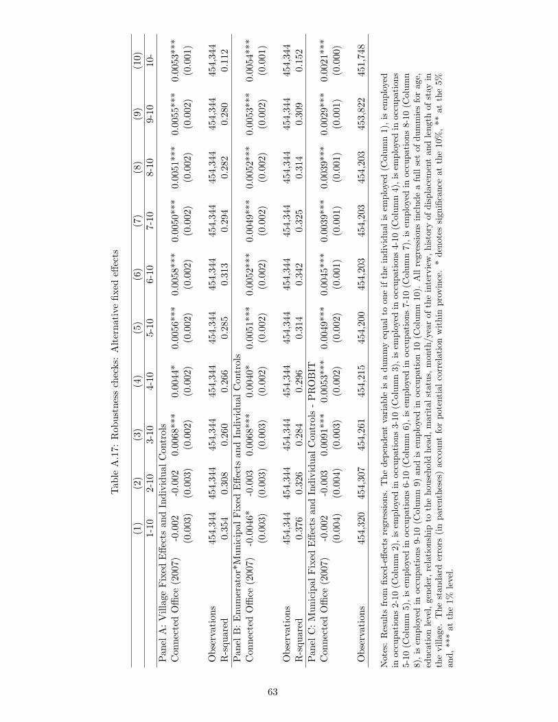
Tab

leA

.17:

Rob

ustn

ess

chec

ks:

Alt

erna

tive

fixed

effec

ts

(1)

(2)

(3)

(4)

(5)

(6)

(7)

(8)

(9)

(10)

1-10

2-10

3-10

4-10

5-10

6-10

7-10

8-10

9-10

10-

Pan

elA

:V

illag

eF

ixed

Effe

cts

and

Indi

vidu

alC

ontr

ols

Con

nect

edO

ffice

(200

7)-0

.002

-0.0

020.

0068

***

0.00

44*

0.00

56**

*0.

0058

***

0.00

50**

*0.

0051

***

0.00

55**

*0.

0053

***

(0.0

03)

(0.0

03)

(0.0

02)

(0.0

02)

(0.0

02)

(0.0

02)

(0.0

02)

(0.0

02)

(0.0

02)

(0.0

01)

Obs

erva

tion

s45

4,34

445

4,34

445

4,34

445

4,34

445

4,34

445

4,34

445

4,34

445

4,34

445

4,34

445

4,34

4R

-squ

ared

0.35

40.

308

0.26

00.

266

0.28

50.

313

0.29

40.

282

0.28

00.

112

Pan

elB

:E

num

erat

or*M

unic

ipal

Fix

edE

ffect

san

dIn

divi

dual

Con

trol

sC

onne

cted

Offi

ce(2

007)

-0.0

046*

-0.0

030.

0068

***

0.00

40*

0.00

51**

*0.

0052

***

0.00

49**

*0.

0052

***

0.00

53**

*0.

0054

***

(0.0

03)

(0.0

03)

(0.0

03)

(0.0

02)

(0.0

02)

(0.0

02)

(0.0

02)

(0.0

02)

(0.0

02)

(0.0

01)

Obs

erva

tion

s45

4,34

445

4,34

445

4,34

445

4,34

445

4,34

445

4,34

445

4,34

445

4,34

445

4,34

445

4,34

4R

-squ

ared

0.37

60.

326

0.28

40.

296

0.31

40.

342

0.32

50.

314

0.30

90.

152

Pan

elC

:M

unic

ipal

Fix

edE

ffect

san

dIn

divi

dual

Con

trol

s-

PR

OB

ITC

onne

cted

Offi

ce(2

007)

-0.0

02-0

.003

0.00

91**

*0.

0053

***

0.00

49**

*0.

0045

***

0.00

39**

*0.

0039

***

0.00

29**

*0.

0021

***

(0.0

04)

(0.0

04)

(0.0

03)

(0.0

02)

(0.0

02)

(0.0

01)

(0.0

01)

(0.0

01)

(0.0

01)

(0.0

00)

Obs

erva

tion

s45

4,32

045

4,30

745

4,26

145

4,21

545

4,20

045

4,20

345

4,20

345

4,20

345

3,82

245

1,74

8

Not

es:

Res

ults

from

fixed

-effe

cts

regr

essi

ons.

The

depe

nden

tva

riab

leis

adu

mm

yeq

ual

toon

eif

the

indi

vidu

alis

empl

oyed

(Col

umn

1),

isem

ploy

edin

occu

pati

ons

2-10

(Col

umn

2),i

sem

ploy

edin

occu

pati

ons

3-10

(Col

umn

3),i

sem

ploy

edin

occu

pati

ons

4-10

(Col

umn

4),i

sem

ploy

edin

occu

pati

ons

5-10

(Col

umn

5),i

sem

ploy

edin

occu

pati

ons

6-10

(Col

umn

6),i

sem

ploy

edin

occu

pati

ons

7-10

(Col

umn

7),i

sem

ploy

edin

occu

pati

ons

8-10

(Col

umn

8),

isem

ploy

edin

occu

pati

ons

9-10

(Col

umn

9)an

dis

empl

oyed

inoc

cupa

tion

10(C

olum

n10

).A

llre

gres

sion

sin

clud

ea

full

set

ofdu

mm

ies

for

age,

educ

atio

nle

vel,

gend

er,r

elat

ions

hip

toth

eho

useh

old

head

,mar

ital

stat

us,m

onth

/yea

rof

the

inte

rvie

w,h

isto

ryof

disp

lace

men

tan

dle

ngth

ofst

ayin

the

villa

ge.

The

stan

dard

erro

rs(i

npa

rent

hese

s)ac

coun

tfo

rpo

tent

ial

corr

elat

ion

wit

hin

prov

ince

.*

deno

tes

sign

ifica

nce

atth

e10

%,

**at

the

5%an

d,**

*at

the

1%le

vel.

63

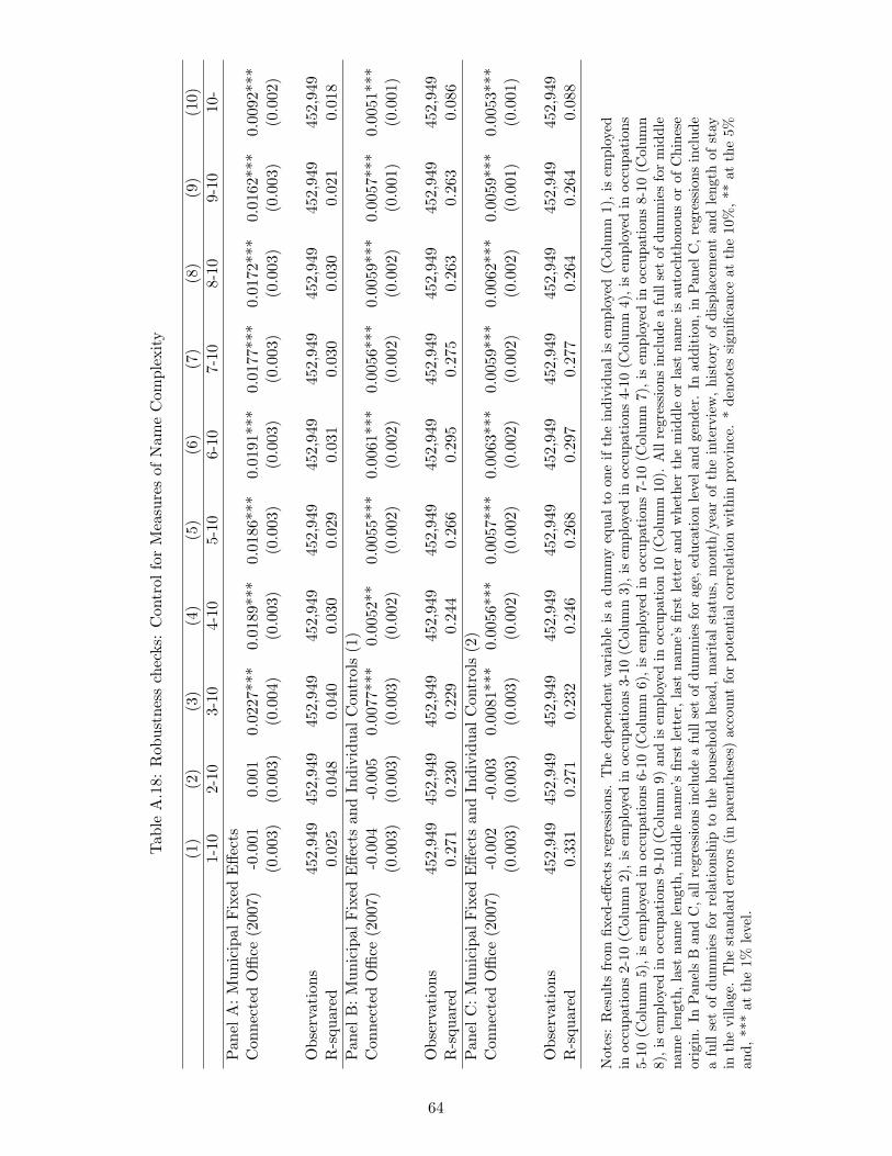
Tab

leA

.18:

Rob

ustn

ess

chec

ks:

Con

trol

for

Mea

sure

sof

Nam

eC

ompl

exit

y

(1)

(2)

(3)

(4)

(5)

(6)

(7)

(8)

(9)

(10)

1-10

2-10

3-10

4-10

5-10

6-10

7-10

8-10

9-10

10-

Pan

elA

:M

unic

ipal

Fix

edE

ffect

sC

onne

cted

Offi

ce(2

007)

-0.0

010.

001

0.02

27**

*0.

0189

***

0.01

86**

*0.

0191

***

0.01

77**

*0.

0172

***

0.01

62**

*0.

0092

***

(0.0

03)

(0.0

03)

(0.0

04)

(0.0

03)

(0.0

03)

(0.0

03)

(0.0

03)

(0.0

03)

(0.0

03)

(0.0

02)

Obs

erva

tion

s45

2,94

945

2,94

945

2,94

945

2,94

945

2,94

945

2,94

945

2,94

945

2,94

945

2,94

945

2,94

9R

-squ

ared

0.02

50.

048

0.04

00.

030

0.02

90.

031

0.03

00.

030

0.02

10.

018

Pan

elB

:M

unic

ipal

Fix

edE

ffect

san

dIn

divi

dual

Con

trol

s(1

)C

onne

cted

Offi

ce(2

007)

-0.0

04-0

.005

0.00

77**

*0.

0052

**0.

0055

***

0.00

61**

*0.

0056

***

0.00

59**

*0.

0057

***

0.00

51**

*(0

.003

)(0

.003

)(0

.003

)(0

.002

)(0

.002

)(0

.002

)(0

.002

)(0

.002

)(0

.001

)(0

.001

)

Obs

erva

tion

s45

2,94

945

2,94

945

2,94

945

2,94

945

2,94

945

2,94

945

2,94

945

2,94

945

2,94

945

2,94

9R

-squ

ared

0.27

10.

230

0.22

90.

244

0.26

60.

295

0.27

50.

263

0.26

30.

086

Pan

elC

:M

unic

ipal

Fix

edE

ffect

san

dIn

divi

dual

Con

trol

s(2

)C

onne

cted

Offi

ce(2

007)

-0.0

02-0

.003

0.00

81**

*0.

0056

***

0.00

57**

*0.

0063

***

0.00

59**

*0.

0062

***

0.00

59**

*0.

0053

***

(0.0

03)

(0.0

03)

(0.0

03)

(0.0

02)

(0.0

02)

(0.0

02)

(0.0

02)

(0.0

02)

(0.0

01)

(0.0

01)

Obs

erva

tion

s45

2,94

945

2,94

945

2,94

945

2,94

945

2,94

945

2,94

945

2,94

945

2,94

945

2,94

945

2,94

9R

-squ

ared

0.33

10.

271

0.23

20.

246

0.26

80.

297

0.27

70.

264

0.26

40.

088

Not

es:

Res

ults

from

fixed

-effe

cts

regr

essi

ons.

The

depe

nden

tva

riab

leis

adu

mm

yeq

ual

toon

eif

the

indi

vidu

alis

empl

oyed

(Col

umn

1),

isem

ploy

edin

occu

pati

ons

2-10

(Col

umn

2),i

sem

ploy

edin

occu

pati

ons

3-10

(Col

umn

3),i

sem

ploy

edin

occu

pati

ons

4-10

(Col

umn

4),i

sem

ploy

edin

occu

pati

ons

5-10

(Col

umn

5),i

sem

ploy

edin

occu

pati

ons

6-10

(Col

umn

6),i

sem

ploy

edin

occu

pati

ons

7-10

(Col

umn

7),i

sem

ploy

edin

occu

pati

ons

8-10

(Col

umn

8),i

sem

ploy

edin

occu

pati

ons

9-10

(Col

umn

9)an

dis

empl

oyed

inoc

cupa

tion

10(C

olum

n10

).A

llre

gres

sion

sin

clud

ea

full

set

ofdu

mm

ies

for

mid

dle

nam

ele

ngth

,las

tna

me

leng

th,m

iddl

ena

me’

sfir

stle

tter

,las

tna

me’

sfir

stle

tter

and

whe

ther

the

mid

dle

orla

stna

me

isau

toch

thon

ous

orof

Chi

nese

orig

in.

InP

anel

sB

and

C,a

llre

gres

sion

sin

clud

ea

full

set

ofdu

mm

ies

for

age,

educ

atio

nle

vela

ndge

nder

.In

addi

tion

,in

Pan

elC

,reg

ress

ions

incl

ude

afu

llse

tof

dum

mie

sfo

rre

lati

onsh

ipto

the

hous

ehol

dhe

ad,

mar

ital

stat

us,

mon

th/y

ear

ofth

ein

terv

iew

,hi

stor

yof

disp

lace

men

tan

dle

ngth

ofst

ayin

the

villa

ge.

The

stan

dard

erro

rs(i

npa

rent

hese

s)ac

coun

tfo

rpo

tent

ialc

orre

lati

onw

ithi

npr

ovin

ce.

*de

note

ssi

gnifi

canc

eat

the

10%

,**

atth

e5%

and,

***

atth

e1%

leve

l.

64

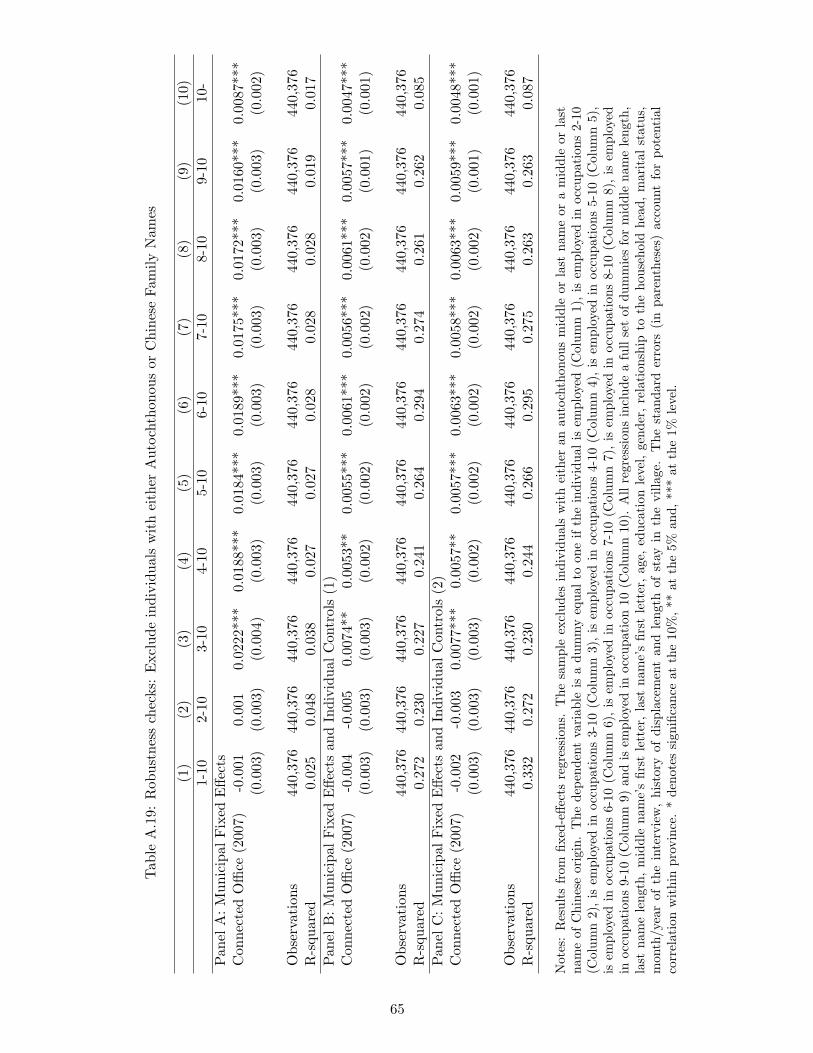
Tab

leA

.19:

Rob

ustn

ess

chec

ks:

Exc

lude

indi

vidu

als

wit

hei

ther

Aut

ocht

hono

usor

Chi

nese

Fam

ilyN

ames

(1)

(2)

(3)

(4)

(5)

(6)

(7)

(8)

(9)

(10)

1-10

2-10

3-10

4-10

5-10

6-10

7-10

8-10

9-10

10-

Pan

elA

:M

unic

ipal

Fix

edE

ffect

sC

onne

cted

Offi

ce(2

007)

-0.0

010.

001

0.02

22**

*0.

0188

***

0.01

84**

*0.

0189

***

0.01

75**

*0.

0172

***

0.01

60**

*0.

0087

***

(0.0

03)

(0.0

03)

(0.0

04)

(0.0

03)

(0.0

03)

(0.0

03)

(0.0

03)

(0.0

03)

(0.0

03)

(0.0

02)

Obs

erva

tion

s44

0,37

644

0,37

644

0,37

644

0,37

644

0,37

644

0,37

644

0,37

644

0,37

644

0,37

644

0,37

6R

-squ

ared

0.02

50.

048

0.03

80.

027

0.02

70.

028

0.02

80.

028

0.01

90.

017

Pan

elB

:M

unic

ipal

Fix

edE

ffect

san

dIn

divi

dual

Con

trol

s(1

)C

onne

cted

Offi

ce(2

007)

-0.0

04-0

.005

0.00

74**

0.00

53**

0.00

55**

*0.

0061

***

0.00

56**

*0.

0061

***

0.00

57**

*0.

0047

***

(0.0

03)

(0.0

03)

(0.0

03)

(0.0

02)

(0.0

02)

(0.0

02)

(0.0

02)

(0.0

02)

(0.0

01)

(0.0

01)

Obs

erva

tion

s44

0,37

644

0,37

644

0,37

644

0,37

644

0,37

644

0,37

644

0,37

644

0,37

644

0,37

644

0,37

6R

-squ

ared

0.27

20.

230

0.22

70.

241

0.26

40.

294

0.27

40.

261

0.26

20.

085

Pan

elC

:M

unic

ipal

Fix

edE

ffect

san

dIn

divi

dual

Con

trol

s(2

)C

onne

cted

Offi

ce(2

007)

-0.0

02-0

.003

0.00

77**

*0.

0057

**0.

0057

***

0.00

63**

*0.

0058

***

0.00

63**

*0.

0059

***

0.00

48**

*(0

.003

)(0

.003

)(0

.003

)(0

.002

)(0

.002

)(0

.002

)(0

.002

)(0

.002

)(0

.001

)(0

.001

)

Obs

erva

tion

s44

0,37

644

0,37

644

0,37

644

0,37

644

0,37

644

0,37

644

0,37

644

0,37

644

0,37

644

0,37

6R

-squ

ared

0.33

20.

272

0.23

00.

244

0.26

60.

295

0.27

50.

263

0.26

30.

087

Not

es:

Res

ults

from

fixed

-effe

cts

regr

essi

ons.

The

sam

ple

excl

udes

indi

vidu

als

wit

hei

ther

anau

toch

thon

ous

mid

dle

orla

stna

me

ora

mid

dle

orla

stna

me

ofC

hine

seor

igin

.T

hede

pend

ent

vari

able

isa

dum

my

equa

lto

one

ifth

ein

divi

dual

isem

ploy

ed(C

olum

n1)

,is

empl

oyed

inoc

cupa

tion

s2-

10(C

olum

n2)

,is

empl

oyed

inoc

cupa

tion

s3-

10(C

olum

n3)

,is

empl

oyed

inoc

cupa

tion

s4-

10(C

olum

n4)

,is

empl

oyed

inoc

cupa

tion

s5-

10(C

olum

n5)

,is

empl

oyed

inoc

cupa

tion

s6-

10(C

olum

n6)

,is

empl

oyed

inoc

cupa

tion

s7-

10(C

olum

n7)

,is

empl

oyed

inoc

cupa

tion

s8-

10(C

olum

n8)

,is

empl

oyed

inoc

cupa

tion

s9-

10(C

olum

n9)

and

isem

ploy

edin

occu

pati

on10

(Col

umn

10).

All

regr

essi

ons

incl

ude

afu

llse

tof

dum

mie

sfo

rm

iddl

ena

me

leng

th,

last

nam

ele

ngth

,m

iddl

ena

me’

sfir

stle

tter

,la

stna

me’

sfir

stle

tter

,ag

e,ed

ucat

ion

leve

l,ge

nder

,re

lati

onsh

ipto

the

hous

ehol

dhe

ad,

mar

ital

stat

us,

mon

th/y

ear

ofth

ein

terv

iew

,hi

stor

yof

disp

lace

men

tan

dle

ngth

ofst

ayin

the

villa

ge.

The

stan

dard

erro

rs(i

npa

rent

hese

s)ac

coun

tfo

rpo

tent

ial

corr

elat

ion

wit

hin

prov

ince

.*

deno

tes

sign

ifica

nce

atth

e10

%,

**at

the

5%an

d,**

*at

the

1%le

vel.

65

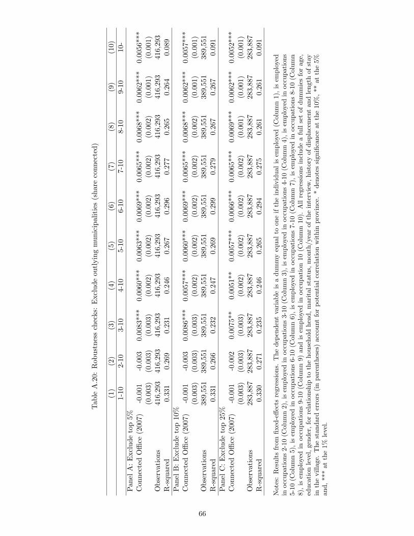
Tab

leA

.20:

Rob

ustn

ess

chec

ks:

Exc

lude

outl

ying

mun

icip

alit

ies

(sha

reco

nnec

ted)

(1)

(2)

(3)

(4)

(5)

(6)

(7)

(8)

(9)

(10)

1-10

2-10

3-10

4-10

5-10

6-10

7-10

8-10

9-10

10-

Pan

elA

:E

xclu

deto

p5%

Con

nect

edO

ffice

(200

7)-0

.001

-0.0

030.

0083

***

0.00

60**

*0.

0063

***

0.00

69**

*0.

0065

***

0.00

68**

*0.

0062

***

0.00

56**

*(0

.003

)(0

.003

)(0

.003

)(0

.002

)(0

.002

)(0

.002

)(0

.002

)(0

.002

)(0

.001

)(0

.001

)O

bser

vati

ons

416,

293

416,

293

416,

293

416,

293

416,

293

416,

293

416,

293

416,

293

416,

293

416,

293

R-s

quar

ed0.

331

0.26

90.

231

0.24

60.

267

0.29

60.

277

0.26

50.

264

0.08

9P

anel

B:

Exc

lude

top

10%

Con

nect

edO

ffice

(200

7)-0

.001

-0.0

030.

0086

***

0.00

57**

*0.

0060

***

0.00

69**

*0.

0065

***

0.00

68**

*0.

0062

***

0.00

57**

*(0

.003

)(0

.003

)(0

.003

)(0

.002

)(0

.002

)(0

.002

)(0

.002

)(0

.002

)(0

.001

)(0

.001

)O

bser

vati

ons

389,

551

389,

551

389,

551

389,

551

389,

551

389,

551

389,

551

389,

551

389,

551

389,

551

R-s

quar

ed0.

331

0.26

60.

232

0.24

70.

269

0.29

90.

279

0.26

70.

267

0.09

1P

anel

C:

Exc

lude

top

25%

Con

nect

edO

ffice

(200

7)-0

.001

-0.0

020.

0075

**0.

0051

**0.

0057

***

0.00

66**

*0.

0065

***

0.00

69**

*0.

0062

***

0.00

52**

*(0

.003

)(0

.003

)(0

.003

)(0

.002

)(0

.002

)(0

.002

)(0

.002

)(0

.001

)(0

.001

)(0

.001

)O

bser

vati

ons

283,

887

283,

887

283,

887

283,

887

283,

887

283,

887

283,

887

283,

887

283,

887

283,

887

R-s

quar

ed0.

330

0.27

10.

235

0.24

60.

265

0.29

40.

275

0.26

10.

261

0.09

1

Not

es:

Res

ults

from

fixed

-effe

cts

regr

essi

ons.

The

depe

nden

tva

riab

leis

adu

mm

yeq

ual

toon

eif

the

indi

vidu

alis

empl

oyed

(Col

umn

1),

isem

ploy

edin

occu

pati

ons

2-10

(Col

umn

2),i

sem

ploy

edin

occu

pati

ons

3-10

(Col

umn

3),i

sem

ploy

edin

occu

pati

ons

4-10

(Col

umn

4),i

sem

ploy

edin

occu

pati

ons

5-10

(Col

umn

5),i

sem

ploy

edin

occu

pati

ons

6-10

(Col

umn

6),i

sem

ploy

edin

occu

pati

ons

7-10

(Col

umn

7),i

sem

ploy

edin

occu

pati

ons

8-10

(Col

umn

8),

isem

ploy

edin

occu

pati

ons

9-10

(Col

umn

9)an

dis

empl

oyed

inoc

cupa

tion

10(C

olum

n10

).A

llre

gres

sion

sin

clud

ea

full

set

ofdu

mm

ies

for

age,

educ

atio

nle

vel,

gend

er,f

orre

lati

onsh

ipto

the

hous

ehol

dhe

ad,m

arit

alst

atus

,mon

th/y

ear

ofth

ein

terv

iew

,his

tory

ofdi

spla

cem

ent

and

leng

thof

stay

inth

evi

llage

.T

hest

anda

rder

rors

(in

pare

nthe

ses)

acco

unt

for

pote

ntia

lcor

rela

tion

wit

hin

prov

ince

.*

deno

tes

sign

ifica

nce

atth

e10

%,*

*at

the

5%an

d,**

*at

the

1%le

vel.

66

Tab

leA

.21:

Rob

ustn

ess

chec

ks:

Exc

lude

outl

ying

mun

icip

alit

ies

(sha

reco

nnec

ted)

(1)

(2)

(3)

(4)

(5)

(6)

(7)

(8)

(9)

(10)

1-10

2-10

3-10

4-10

5-10

6-10

7-10

8-10

9-10

10-

Pan

elA

:E

xclu

debo

ttom

5%C

onne

cted

Offi

ce(2

007)

-0.0

01-0

.003

0.00

89**

*0.

0064

***

0.00

64**

*0.

0067

***

0.00

62**

*0.

0064

***

0.00

63**

*0.

0055

***

(0.0

03)

(0.0

03)

(0.0

03)

(0.0

02)

(0.0

02)

(0.0

02)

(0.0

02)

(0.0

02)

(0.0

02)

(0.0

01)

Obs

erva

tion

s44

7,57

244

7,57

244

7,57

244

7,57

244

7,57

244

7,57

244

7,57

244

7,57

244

7,57

244

7,57

2R

-squ

ared

0.33

10.

271

0.23

20.

246

0.26

90.

297

0.27

70.

265

0.26

40.

088

Pan

elB

:E

xclu

debo

ttom

10%

Con

nect

edO

ffice

(200

7)-0

.001

-0.0

030.

0087

***

0.00

60**

*0.

0058

***

0.00

61**

*0.

0055

***

0.00

59**

*0.

0061

***

0.00

55**

*(0

.003

)(0

.003

)(0

.003

)(0

.002

)(0

.002

)(0

.002

)(0

.002

)(0

.002

)(0

.002

)(0

.001

)O

bser

vati

ons

438,

037

438,

037

438,

037

438,

037

438,

037

438,

037

438,

037

438,

037

438,

037

438,

037

R-s

quar

ed0.

331

0.27

00.

231

0.24

60.

268

0.29

70.

277

0.26

50.

264

0.08

7P

anel

C:

Exc

lude

bott

om25

%C

onne

cted

Offi

ce(2

007)

-0.0

01-0

.003

0.00

95**

*0.

0059

***

0.00

60**

*0.

0063

***

0.00

56**

*0.

0061

***

0.00

65**

*0.

0064

***

(0.0

03)

(0.0

04)

(0.0

03)

(0.0

02)

(0.0

02)

(0.0

02)

(0.0

02)

(0.0

02)

(0.0

02)

(0.0

01)

Obs

erva

tion

s39

2,00

739

2,00

739

2,00

739

2,00

739

2,00

739

2,00

739

2,00

739

2,00

739

2,00

739

2,00

7R

-squ

ared

0.33

10.

269

0.22

80.

243

0.26

60.

294

0.27

40.

262

0.26

10.

083

Not

es:

Res

ults

from

fixed

-effe

cts

regr

essi

ons.

The

depe

nden

tva

riab

leis

adu

mm

yeq

ual

toon

eif

the

indi

vidu

alis

empl

oyed

(Col

umn

1),

isem

ploy

edin

occu

pati

ons

2-10

(Col

umn

2),i

sem

ploy

edin

occu

pati

ons

3-10

(Col

umn

3),i

sem

ploy

edin

occu

pati

ons

4-10

(Col

umn

4),i

sem

ploy

edin

occu

pati

ons

5-10

(Col

umn

5),i

sem

ploy

edin

occu

pati

ons

6-10

(Col

umn

6),i

sem

ploy

edin

occu

pati

ons

7-10

(Col

umn

7),i

sem

ploy

edin

occu

pati

ons

8-10

(Col

umn

8),

isem

ploy

edin

occu

pati

ons

9-10

(Col

umn

9)an

dis

empl

oyed

inoc

cupa

tion

10(C

olum

n10

).A

llre

gres

sion

sin

clud

ea

full

set

ofdu

mm

ies

for

age,

educ

atio

nle

vel,

gend

er,f

orre

lati

onsh

ipto

the

hous

ehol

dhe

ad,m

arit

alst

atus

,mon

th/y

ear

ofth

ein

terv

iew

,his

tory

ofdi

spla

cem

ent

and

leng

thof

stay

inth

evi

llage

.T

hest

anda

rder

rors

(in

pare

nthe

ses)

acco

unt

for

pote

ntia

lcor

rela

tion

wit

hin

prov

ince

.*

deno

tes

sign

ifica

nce

atth

e10

%,*

*at

the

5%an

d,**

*at

the

1%le

vel.

67

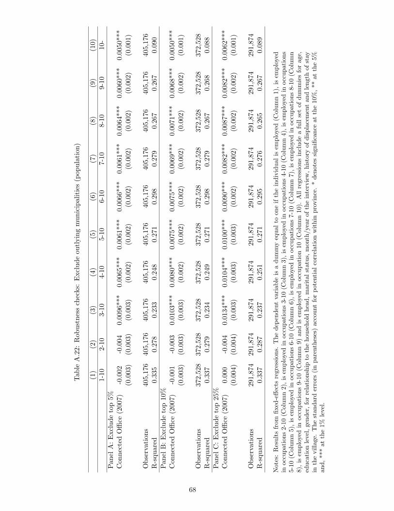
Tab

leA

.22:

Rob

ustn

ess

chec

ks:

Exc

lude

outl

ying

mun

icip

alit

ies

(pop

ulat

ion)

(1)

(2)

(3)

(4)

(5)

(6)

(7)

(8)

(9)

(10)

1-10

2-10

3-10

4-10

5-10

6-10

7-10

8-10

9-10

10-

Pan

elA

:E

xclu

deto

p5%

Con

nect

edO

ffice

(200

7)-0

.002

-0.0

040.

0096

***

0.00

65**

*0.

0061

***

0.00

66**

*0.

0061

***

0.00

64**

*0.

0060

***

0.00

50**

*(0

.003

)(0

.003

)(0

.003

)(0

.002

)(0

.002

)(0

.002

)(0

.002

)(0

.002

)(0

.002

)(0

.001

)

Obs

erva

tion

s40

5,17

640

5,17

640

5,17

640

5,17

640

5,17

640

5,17

640

5,17

640

5,17

640

5,17

640

5,17

6R

-squ

ared

0.33

50.

278

0.23

30.

248

0.27

10.

298

0.27

90.

267

0.26

70.

090

Pan

elB

:E

xclu

deto

p10

%C

onne

cted

Offi

ce(2

007)

-0.0

01-0

.003

0.01

03**

*0.

0080

***

0.00

75**

*0.

0075

***

0.00

69**

*0.

0071

***

0.00

68**

*0.

0050

***

(0.0

03)

(0.0

03)

(0.0

03)

(0.0

02)

(0.0

02)

(0.0

02)

(0.0

02)

(0.0

02)

(0.0

02)

(0.0

01)

Obs

erva

tion

s37

2,52

837

2,52

837

2,52

837

2,52

837

2,52

837

2,52

837

2,52

837

2,52

837

2,52

837

2,52

8R

-squ

ared

0.33

70.

279

0.23

40.

249

0.27

10.

298

0.27

90.

267

0.26

80.

088

Pan

elC

:E

xclu

deto

p25

%C

onne

cted

Offi

ce(2

007)

0.00

0-0

.004

0.01

34**

*0.

0104

***

0.01

00**

*0.

0090

***

0.00

82**

*0.

0087

***

0.00

82**

*0.

0062

***

(0.0

04)

(0.0

04)

(0.0

03)

(0.0

03)

(0.0

03)

(0.0

02)

(0.0

02)

(0.0

02)

(0.0

02)

(0.0

01)

Obs

erva

tion

s29

1,87

429

1,87

429

1,87

429

1,87

429

1,87

429

1,87

429

1,87

429

1,87

429

1,87

429

1,87

4R

-squ

ared

0.33

70.

287

0.23

70.

251

0.27

10.

295

0.27

60.

265

0.26

70.

089

Not

es:

Res

ults

from

fixed

-effe

cts

regr

essi

ons.

The

depe

nden

tva

riab

leis

adu

mm

yeq

ual

toon

eif

the

indi

vidu

alis

empl

oyed

(Col

umn

1),

isem

ploy

edin

occu

pati

ons

2-10

(Col

umn

2),i

sem

ploy

edin

occu

pati

ons

3-10

(Col

umn

3),i

sem

ploy

edin

occu

pati

ons

4-10

(Col

umn

4),i

sem

ploy

edin

occu

pati

ons

5-10

(Col

umn

5),i

sem

ploy

edin

occu

pati

ons

6-10

(Col

umn

6),i

sem

ploy

edin

occu

pati

ons

7-10

(Col

umn

7),i

sem

ploy

edin

occu

pati

ons

8-10

(Col

umn

8),

isem

ploy

edin

occu

pati

ons

9-10

(Col

umn

9)an

dis

empl

oyed

inoc

cupa

tion

10(C

olum

n10

).A

llre

gres

sion

sin

clud

ea

full

set

ofdu

mm

ies

for

age,

educ

atio

nle

vel,

gend

er,f

orre

lati

onsh

ipto

the

hous

ehol

dhe

ad,m

arit

alst

atus

,mon

th/y

ear

ofth

ein

terv

iew

,his

tory

ofdi

spla

cem

ent

and

leng

thof

stay

inth

evi

llage

.T

hest

anda

rder

rors

(in

pare

nthe

ses)

acco

unt

for

pote

ntia

lcor

rela

tion

wit

hin

prov

ince

.*

deno

tes

sign

ifica

nce

atth

e10

%,*

*at

the

5%an

d,**

*at

the

1%le

vel.

68

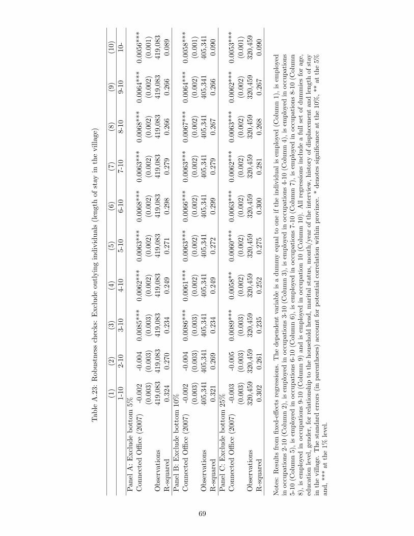
Tab

leA

.23:

Rob

ustn

ess

chec

ks:

Exc

lude

outl

ying

indi

vidu

als

(len

gth

ofst

ayin

the

villa

ge)

(1)

(2)

(3)

(4)

(5)

(6)

(7)

(8)

(9)

(10)

1-10

2-10

3-10

4-10

5-10

6-10

7-10

8-10

9-10

10-

Pan

elA

:E

xclu

debo

ttom

5%C

onne

cted

Offi

ce(2

007)

-0.0

02-0

.004

0.00

85**

*0.

0062

***

0.00

63**

*0.

0068

***

0.00

63**

*0.

0068

***

0.00

64**

*0.

0056

***

(0.0

03)

(0.0

03)

(0.0

03)

(0.0

02)

(0.0

02)

(0.0

02)

(0.0

02)

(0.0

02)

(0.0

02)

(0.0

01)

Obs

erva

tion

s41

9,08

341

9,08

341

9,08

341

9,08

341

9,08

341

9,08

341

9,08

341

9,08

341

9,08

341

9,08

3R

-squ

ared

0.32

40.

270

0.23

40.

249

0.27

10.

298

0.27

90.

266

0.26

60.

089

Pan

elB

:E

xclu

debo

ttom

10%

Con

nect

edO

ffice

(200

7)-0

.002

-0.0

040.

0086

***

0.00

61**

*0.

0063

***

0.00

66**

*0.

0063

***

0.00

67**

*0.

0064

***

0.00

58**

*(0

.003

)(0

.003

)(0

.003

)(0

.002

)(0

.002

)(0

.002

)(0

.002

)(0

.002

)(0

.002

)(0

.001

)O

bser

vati

ons

405,

341

405,

341

405,

341

405,

341

405,

341

405,

341

405,

341

405,

341

405,

341

405,

341

R-s

quar

ed0.

321

0.26

90.

234

0.24

90.

272

0.29

90.

279

0.26

70.

266

0.09

0P

anel

C:

Exc

lude

bott

om25

%C

onne

cted

Offi

ce(2

007)

-0.0

03-0

.005

0.00

89**

*0.

0058

**0.

0060

***

0.00

63**

*0.

0062

***

0.00

63**

*0.

0062

***

0.00

53**

*(0

.003

)(0

.003

)(0

.003

)(0

.002

)(0

.002

)(0

.002

)(0

.002

)(0

.002

)(0

.002

)(0

.001

)O

bser

vati

ons

320,

459

320,

459

320,

459

320,

459

320,

459

320,

459

320,

459

320,

459

320,

459

320,

459

R-s

quar

ed0.

302

0.26

10.

235

0.25

20.

275

0.30

00.

281

0.26

80.

267

0.09

0

Not

es:

Res

ults

from

fixed

-effe

cts

regr

essi

ons.

The

depe

nden

tva

riab

leis

adu

mm

yeq

ual

toon

eif

the

indi

vidu

alis

empl

oyed

(Col

umn

1),

isem

ploy

edin

occu

pati

ons

2-10

(Col

umn

2),i

sem

ploy

edin

occu

pati

ons

3-10

(Col

umn

3),i

sem

ploy

edin

occu

pati

ons

4-10

(Col

umn

4),i

sem

ploy

edin

occu

pati

ons

5-10

(Col

umn

5),i

sem

ploy

edin

occu

pati

ons

6-10

(Col

umn

6),i

sem

ploy

edin

occu

pati

ons

7-10

(Col

umn

7),i

sem

ploy

edin

occu

pati

ons

8-10

(Col

umn

8),

isem

ploy

edin

occu

pati

ons

9-10

(Col

umn

9)an

dis

empl

oyed

inoc

cupa

tion

10(C

olum

n10

).A

llre

gres

sion

sin

clud

ea

full

set

ofdu

mm

ies

for

age,

educ

atio

nle

vel,

gend

er,f

orre

lati

onsh

ipto

the

hous

ehol

dhe

ad,m

arit

alst

atus

,mon

th/y

ear

ofth

ein

terv

iew

,his

tory

ofdi

spla

cem

ent

and

leng

thof

stay

inth

evi

llage

.T

hest

anda

rder

rors

(in

pare

nthe

ses)

acco

unt

for

pote

ntia

lcor

rela

tion

wit

hin

prov

ince

.*

deno

tes

sign

ifica

nce

atth

e10

%,*

*at

the

5%an

d,**

*at

the

1%le

vel.

69

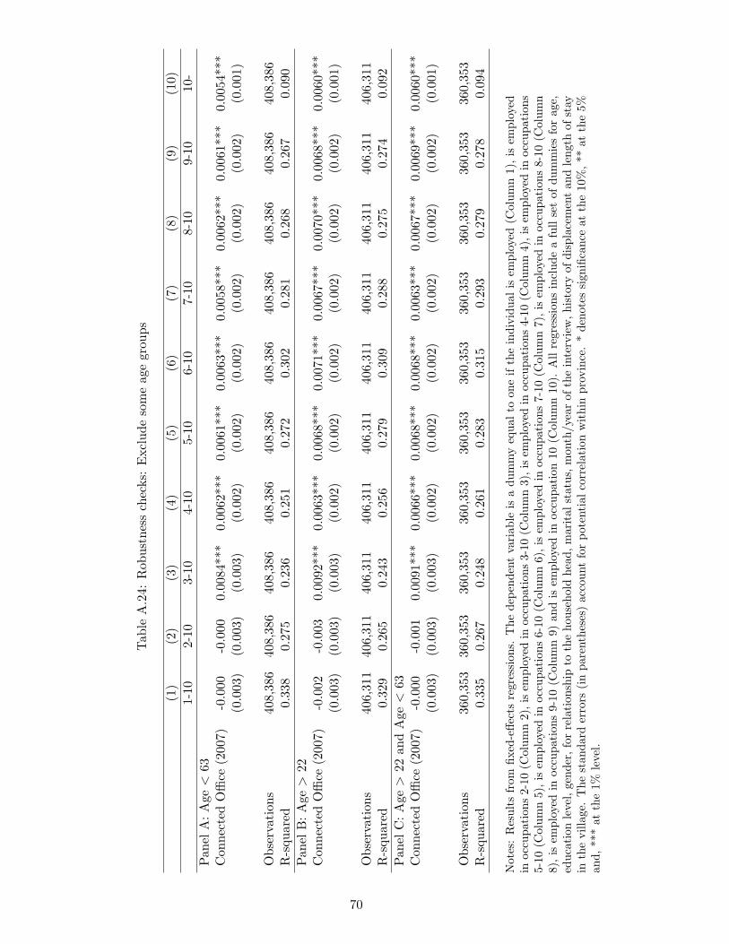
Tab

leA

.24:

Rob

ustn

ess

chec

ks:

Exc

lude

som

eag

egr

oups

(1)

(2)

(3)

(4)

(5)

(6)

(7)

(8)

(9)

(10)

1-10

2-10

3-10

4-10

5-10

6-10

7-10

8-10

9-10

10-

Pan

elA

:A

ge<

63C

onne

cted

Offi

ce(2

007)

-0.0

00-0

.000

0.00

84**

*0.

0062

***

0.00

61**

*0.

0063

***

0.00

58**

*0.

0062

***

0.00

61**

*0.

0054

***

(0.0

03)

(0.0

03)

(0.0

03)

(0.0

02)

(0.0

02)

(0.0

02)

(0.0

02)

(0.0

02)

(0.0

02)

(0.0

01)

Obs

erva

tion

s40

8,38

640

8,38

640

8,38

640

8,38

640

8,38

640

8,38

640

8,38

640

8,38

640

8,38

640

8,38

6R

-squ

ared

0.33

80.

275

0.23

60.

251

0.27

20.

302

0.28

10.

268

0.26

70.

090

Pan

elB

:A

ge>

22C

onne

cted

Offi

ce(2

007)

-0.0

02-0

.003

0.00

92**

*0.

0063

***

0.00

68**

*0.

0071

***

0.00

67**

*0.

0070

***

0.00

68**

*0.

0060

***

(0.0

03)

(0.0

03)

(0.0

03)

(0.0

02)

(0.0

02)

(0.0

02)

(0.0

02)

(0.0

02)

(0.0

02)

(0.0

01)

Obs

erva

tion

s40

6,31

140

6,31

140

6,31

140

6,31

140

6,31

140

6,31

140

6,31

140

6,31

140

6,31

140

6,31

1R

-squ

ared

0.32

90.

265

0.24

30.

256

0.27

90.

309

0.28

80.

275

0.27

40.

092

Pan

elC

:A

ge>

22an

dA

ge<

63C

onne

cted

Offi

ce(2

007)

-0.0

00-0

.001

0.00

91**

*0.

0066

***

0.00

68**

*0.

0068

***

0.00

63**

*0.

0067

***

0.00

69**

*0.

0060

***

(0.0

03)

(0.0

03)

(0.0

03)

(0.0

02)

(0.0

02)

(0.0

02)

(0.0

02)

(0.0

02)

(0.0

02)

(0.0

01)

Obs

erva

tion

s36

0,35

336

0,35

336

0,35

336

0,35

336

0,35

336

0,35

336

0,35

336

0,35

336

0,35

336

0,35

3R

-squ

ared

0.33

50.

267

0.24

80.

261

0.28

30.

315

0.29

30.

279

0.27

80.

094

Not

es:

Res

ults

from

fixed

-effe

cts

regr

essi

ons.

The

depe

nden

tva

riab

leis

adu

mm

yeq

ual

toon

eif

the

indi

vidu

alis

empl

oyed

(Col

umn

1),

isem

ploy

edin

occu

pati

ons

2-10

(Col

umn

2),i

sem

ploy

edin

occu

pati

ons

3-10

(Col

umn

3),i

sem

ploy

edin

occu

pati

ons

4-10

(Col

umn

4),i

sem

ploy

edin

occu

pati

ons

5-10

(Col

umn

5),i

sem

ploy

edin

occu

pati

ons

6-10

(Col

umn

6),i

sem

ploy

edin

occu

pati

ons

7-10

(Col

umn

7),i

sem

ploy

edin

occu

pati

ons

8-10

(Col

umn

8),

isem

ploy

edin

occu

pati

ons

9-10

(Col

umn

9)an

dis

empl

oyed

inoc

cupa

tion

10(C

olum

n10

).A

llre

gres

sion

sin

clud

ea

full

set

ofdu

mm

ies

for

age,

educ

atio

nle

vel,

gend

er,f

orre

lati

onsh

ipto

the

hous

ehol

dhe

ad,m

arit

alst

atus

,mon

th/y

ear

ofth

ein

terv

iew

,his

tory

ofdi

spla

cem

ent

and

leng

thof

stay

inth

evi

llage

.T

hest

anda

rder

rors

(in

pare

nthe

ses)

acco

unt

for

pote

ntia

lcor

rela

tion

wit

hin

prov

ince

.*

deno

tes

sign

ifica

nce

atth

e10

%,*

*at

the

5%an

d,**

*at

the

1%le

vel.

70

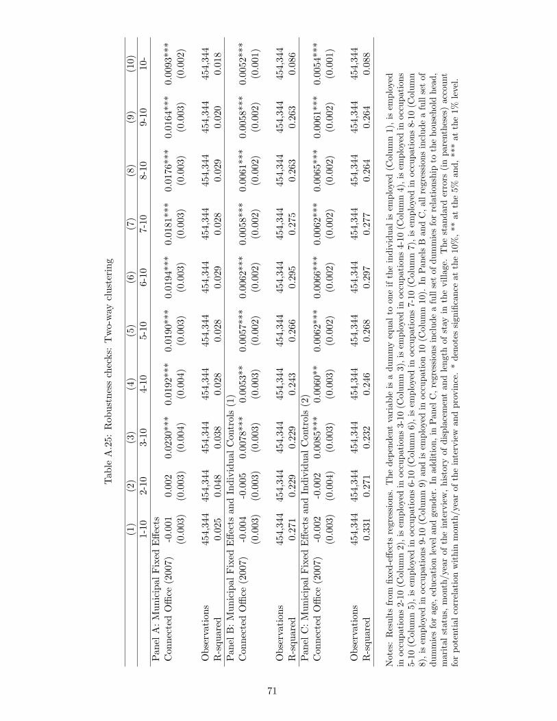
Tab

leA

.25:

Rob

ustn

ess

chec

ks:

Tw

o-w

aycl

uste

ring

(1)

(2)

(3)

(4)

(5)

(6)

(7)

(8)

(9)

(10)

1-10

2-10

3-10

4-10

5-10

6-10

7-10

8-10

9-10

10-

Pan

elA

:M

unic

ipal

Fix

edE

ffect

sC

onne

cted

Offi

ce(2

007)

-0.0

010.

002

0.02

30**

*0.

0192

***

0.01

90**

*0.

0194

***

0.01

81**

*0.

0176

***

0.01

64**

*0.

0093

***

(0.0

03)

(0.0

03)

(0.0

04)

(0.0

04)

(0.0

03)

(0.0

03)

(0.0

03)

(0.0

03)

(0.0

03)

(0.0

02)

Obs

erva

tion

s45

4,34

445

4,34

445

4,34

445

4,34

445

4,34

445

4,34

445

4,34

445

4,34

445

4,34

445

4,34

4R

-squ

ared

0.02

50.

048

0.03

80.

028

0.02

80.

029

0.02

80.

029

0.02

00.

018

Pan

elB

:M

unic

ipal

Fix

edE

ffect

san

dIn

divi

dual

Con

trol

s(1

)C

onne

cted

Offi

ce(2

007)

-0.0

04-0

.005

0.00

78**

*0.

0053

**0.

0057

***

0.00

62**

*0.

0058

***

0.00

61**

*0.

0058

***

0.00

52**

*(0

.003

)(0

.003

)(0

.003

)(0

.003

)(0

.002

)(0

.002

)(0

.002

)(0

.002

)(0

.002

)(0

.001

)

Obs

erva

tion

s45

4,34

445

4,34

445

4,34

445

4,34

445

4,34

445

4,34

445

4,34

445

4,34

445

4,34

445

4,34

4R

-squ

ared

0.27

10.

229

0.22

90.

243

0.26

60.

295

0.27

50.

263

0.26

30.

086

Pan

elC

:M

unic

ipal

Fix

edE

ffect

san

dIn

divi

dual

Con

trol

s(2

)C

onne

cted

Offi

ce(2

007)

-0.0

02-0

.002

0.00

85**

*0.

0060

**0.

0062

***

0.00

66**

*0.

0062

***

0.00

65**

*0.

0061

***

0.00

54**

*(0

.003

)(0

.004

)(0

.003

)(0

.003

)(0

.002

)(0

.002

)(0

.002

)(0

.002

)(0

.002

)(0

.001

)

Obs

erva

tion

s45

4,34

445

4,34

445

4,34

445

4,34

445

4,34

445

4,34

445

4,34

445

4,34

445

4,34

445

4,34

4R

-squ

ared

0.33

10.

271

0.23

20.

246

0.26

80.

297

0.27

70.

264

0.26

40.

088

Not

es:

Res

ults

from

fixed

-effe

cts

regr

essi

ons.

The

depe

nden

tva

riab

leis

adu

mm

yeq

ual

toon

eif

the

indi

vidu

alis

empl

oyed

(Col

umn

1),

isem

ploy

edin

occu

pati

ons

2-10

(Col

umn

2),i

sem

ploy

edin

occu

pati

ons

3-10

(Col

umn

3),i

sem

ploy

edin

occu

pati

ons

4-10

(Col

umn

4),i

sem

ploy

edin

occu

pati

ons

5-10

(Col

umn

5),i

sem

ploy

edin

occu

pati

ons

6-10

(Col

umn

6),i

sem

ploy

edin

occu

pati

ons

7-10

(Col

umn

7),i

sem

ploy

edin

occu

pati

ons

8-10

(Col

umn

8),i

sem

ploy

edin

occu

pati

ons

9-10

(Col

umn

9)an

dis

empl

oyed

inoc

cupa

tion

10(C

olum

n10

).In

Pan

els

Ban

dC

,all

regr

essi

ons

incl

ude

afu

llse

tof

dum

mie

sfo

rag

e,ed

ucat

ion

leve

land

gend

er.

Inad

diti

on,i

nP

anel

C,r

egre

ssio

nsin

clud

ea

full

set

ofdu

mm

ies

for

rela

tion

ship

toth

eho

useh

old

head

,m

arit

alst

atus

,m

onth

/yea

rof

the

inte

rvie

w,

hist

ory

ofdi

spla

cem

ent

and

leng

thof

stay

inth

evi

llage

.T

hest

anda

rder

rors

(in

pare

nthe

ses)

acco

unt

for

pote

ntia

lco

rrel

atio

nw

ithi

nm

onth

/yea

rof

the

inte

rvie

wan

dpr

ovin

ce.

*de

note

ssi

gnifi

canc

eat

the

10%

,**

atth

e5%

and,

***

atth

e1%

leve

l.

71

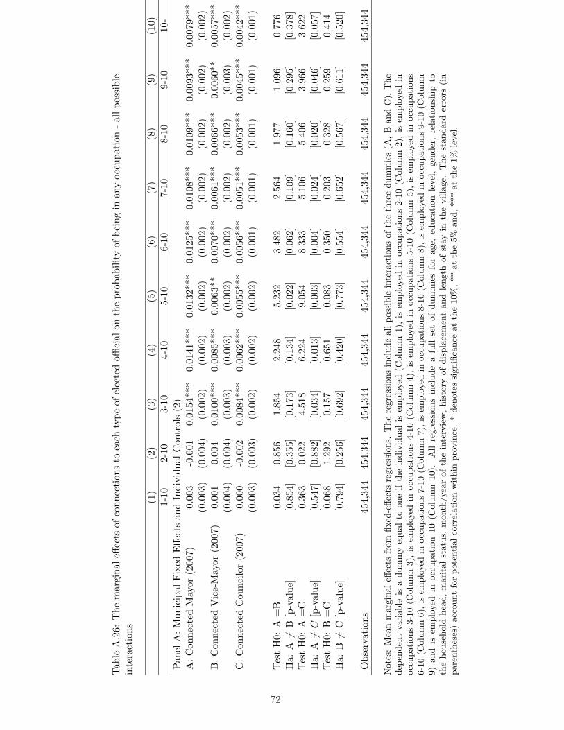
Tab

leA

.26:

The

mar

gina

leffe

cts

ofco

nnec

tion

sto

each

type

ofel

ecte

doffi

cial

onth

epr

obab

ility

ofbe

ing

inan

yoc

cupa

tion

-al

lpos

sibl

ein

tera

ctio

ns

(1)

(2)

(3)

(4)

(5)

(6)

(7)

(8)

(9)

(10)

1-10

2-10

3-10

4-10

5-10

6-10

7-10

8-10

9-10

10-

Pan

elA

:M

unic

ipal

Fix

edE

ffect

san

dIn

divi

dual

Con

trol

s(2

)A

:C

onne

cted

May

or(2

007)

0.00

3-0

.001

0.01

54**

*0.

0141

***

0.01

32**

*0.

0125

***

0.01

08**

*0.

0109

***

0.00

93**

*0.

0079

***

(0.0

03)

(0.0

04)

(0.0

02)

(0.0

02)

(0.0

02)

(0.0

02)

(0.0

02)

(0.0

02)

(0.0

02)

(0.0

02)

B:

Con

nect

edV

ice-

May

or(2

007)

0.00

10.

004

0.01

00**

*0.

0085

***

0.00

63**

0.00

70**

*0.

0061

***

0.00

66**

*0.

0060

**0.

0057

***

(0.0

04)

(0.0

04)

(0.0

03)

(0.0

03)

(0.0

02)

(0.0

02)

(0.0

02)

(0.0

02)

(0.0

03)

(0.0

02)

C:

Con

nect

edC

ounc

ilor

(200

7)0.

000

-0.0

020.

0084

***

0.00

62**

*0.

0055

***

0.00

56**

*0.

0051

***

0.00

53**

*0.

0045

***

0.00

42**

*(0

.003

)(0

.003

)(0

.002

)(0

.002

)(0

.002

)(0

.001

)(0

.001

)(0

.001

)(0

.001

)(0

.001

)

Tes

tH

0:A

=B

0.03

40.

856

1.85

42.

248

5.23

23.

482

2.56

41.

977

1.09

60.

776

Ha:

A6=

B[p

-val

ue]

[0.8

54]

[0.3

55]

[0.1

73]

[0.1

34]

[0.0

22]

[0.0

62]

[0.1

09]

[0.1

60]

[0.2

95]

[0.3

78]

Tes

tH

0:A

=C

0.36

30.

022

4.51

86.

224

9.05

48.

333

5.10

65.

406

3.96

63.

622

Ha:

A6=C

[p-v

alue

][0

.547

][0

.882

][0

.034

][0

.013

][0

.003

][0

.004

][0

.024

][0

.020

][0

.046

][0

.057

]T

est

H0:

B=

C0.

068

1.29

20.

157

0.65

10.

083

0.35

00.

203

0.32

80.

259

0.41

4H

a:B6=

C[p

-val

ue]

[0.7

94]

[0.2

56]

[0.6

92]

[0.4

20]

[0.7

73]

[0.5

54]

[0.6

52]

[0.5

67]

[0.6

11]

[0.5

20]

Obs

erva

tion

s45

4,34

445

4,34

445

4,34

445

4,34

445

4,34

445

4,34

445

4,34

445

4,34

445

4,34

445

4,34

4

Not

es:

Mea

nm

argi

nal

effec

tsfr

omfix

ed-e

ffect

sre

gres

sion

s.T

here

gres

sion

sin

clud

eal

lpo

ssib

lein

tera

ctio

nsof

the

thre

edu

mm

ies

(A,

Ban

dC

).T

hede

pend

ent

vari

able

isa

dum

my

equa

lto

one

ifth

ein

divi

dual

isem

ploy

ed(C

olum

n1)

,is

empl

oyed

inoc

cupa

tion

s2-

10(C

olum

n2)

,is

empl

oyed

inoc

cupa

tion

s3-

10(C

olum

n3)

,is

empl

oyed

inoc

cupa

tion

s4-

10(C

olum

n4)

,is

empl

oyed

inoc

cupa

tion

s5-

10(C

olum

n5)

,is

empl

oyed

inoc

cupa

tion

s6-

10(C

olum

n6)

,is

empl

oyed

inoc

cupa

tion

s7-

10(C

olum

n7)

,is

empl

oyed

inoc

cupa

tion

s8-

10(C

olum

n8)

,is

empl

oyed

inoc

cupa

tion

s9-

10(C

olum

n9)

and

isem

ploy

edin

occu

pati

on10

(Col

umn

10).

All

regr

essi

ons

incl

ude

afu

llse

tof

dum

mie

sfo

rag

e,ed

ucat

ion

leve

l,ge

nder

,re

lati

onsh

ipto

the

hous

ehol

dhe

ad,

mar

ital

stat

us,

mon

th/y

ear

ofth

ein

terv

iew

,hi

stor

yof

disp

lace

men

tan

dle

ngth

ofst

ayin

the

villa

ge.

The

stan

dard

erro

rs(i

npa

rent

hese

s)ac

coun

tfo

rpo

tent

ial

corr

elat

ion

wit

hin

prov

ince

.*

deno

tes

sign

ifica

nce

atth

e10

%,

**at

the

5%an

d,**

*at

the

1%le

vel.

72

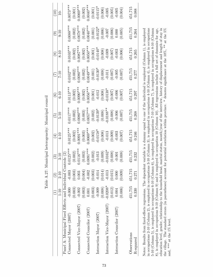
Tab

leA

.27:

Mun

icip

alhe

tero

gene

ity:

Mun

icip

alco

unci

l

(1)

(2)

(3)

(4)

(5)

(6)

(7)

(8)

(9)

(10)

1-10

2-10

3-10

4-10

5-10

6-10

7-10

8-10

9-10

10-

Pan

elA

:M

unic

ipal

Fix

edE

ffect

san

dIn

divi

dual

Con

trol

s(2

)C

onne

cted

May

or(2

007)

-0.0

00-0

.003

0.01

25**

*0.

0125

***

0.01

17**

*0.

0113

***

0.01

02**

*0.

0103

***

0.00

88**

*0.

0073

***

(0.0

03)

(0.0

03)

(0.0

02)

(0.0

02)

(0.0

02)

(0.0

02)

(0.0

02)

(0.0

02)

(0.0

02)

(0.0

01)

Con

nect

edV

ice-

May

or(2

007)

-0.0

020.

003

0.01

16**

*0.

0091

***

0.00

80**

*0.

0090

***

0.00

80**

*0.

0087

***

0.00

78**

*0.

0069

***

(0.0

03)

(0.0

04)

(0.0

03)

(0.0

03)

(0.0

03)

(0.0

02)

(0.0

02)

(0.0

02)

(0.0

02)

(0.0

02)

Con

nect

edC

ounc

ilor

(200

7)0.

001

-0.0

020.

0091

***

0.00

69**

*0.

0057

***

0.00

56**

*0.

0049

***

0.00

50**

*0.

0040

***

0.00

40**

*(0

.003

)(0

.003

)(0

.002

)(0

.002

)(0

.002

)(0

.001

)(0

.001

)(0

.001

)(0

.001

)(0

.001

)In

tera

ctio

nM

ayor

(200

7)-0

.009

-0.0

14-0

.013

-0.0

158*

-0.0

139*

-0.0

12-0

.013

0*-0

.014

0*-0

.012

2*-0

.011

5*(0

.008

)(0

.014

)(0

.009

)(0

.008

)(0

.008

)(0

.008

)(0

.008

)(0

.008

)(0

.006

)(0

.006

)In

tera

ctio

nV

ice-

May

or(2

007)

-0.0

208*

-0.0

13-0

.016

2*-0

.013

-0.0

188*

*-0

.013

8*-0

.011

-0.0

09-0

.007

-0.0

05(0

.012

)(0

.015

)(0

.008

)(0

.009

)(0

.008

)(0

.007

)(0

.007

)(0

.007

)(0

.006

)(0

.005

)In

tera

ctio

nC

ounc

ilor

(200

7)0.

004

0.00

0-0

.001

-0.0

03-0

.006

-0.0

06-0

.005

-0.0

030.

000

-0.0

05(0

.006

)(0

.009

)(0

.008

)(0

.007

)(0

.007

)(0

.007

)(0

.007

)(0

.006

)(0

.005

)(0

.004

)

Obs

erva

tion

s45

1,71

545

1,71

545

1,71

545

1,71

545

1,71

545

1,71

545

1,71

545

1,71

545

1,71

545

1,71

5R

-squ

ared

0.33

00.

271

0.23

20.

246

0.26

80.

297

0.27

70.

265

0.26

40.

088

Not

es:

Res

ults

from

fixed

-effe

cts

regr

essi

ons.

The

depe

nden

tva

riab

leis

adu

mm

yeq

ual

toon

eif

the

indi

vidu

alis

empl

oyed

(Col

umn

1),

isem

ploy

edin

occu

pati

ons

2-10

(Col

umn

2),i

sem

ploy

edin

occu

pati

ons

3-10

(Col

umn

3),i

sem

ploy

edin

occu

pati

ons

4-10

(Col

umn

4),i

sem

ploy

edin

occu

pati

ons

5-10

(Col

umn

5),i

sem

ploy

edin

occu

pati

ons

6-10

(Col

umn

6),i

sem

ploy

edin

occu

pati

ons

7-10

(Col

umn

7),i

sem

ploy

edin

occu

pati

ons

8-10

(Col

umn

8),

isem

ploy

edin

occu

pati

ons

9-10

(Col

umn

9)an

dis

empl

oyed

inoc

cupa

tion

10(C

olum

n10

).A

llre

gres

sion

sin

clud

ea

full

set

ofdu

mm

ies

for

age,

educ

atio

nle

vel,

gend

er,r

elat

ions

hip

toth

eho

useh

old

head

,mar

ital

stat

us,m

onth

/yea

rof

the

inte

rvie

w,h

isto

ryof

disp

lace

men

tan

dle

ngth

ofst

ayin

the

villa

ge.

The

stan

dard

erro

rs(i

npa

rent

hese

s)ac

coun

tfo

rpo

tent

ial

corr

elat

ion

wit

hin

prov

ince

.*

deno

tes

sign

ifica

nce

atth

e10

%,

**at

the

5%an

d,**

*at

the

1%le

vel.

73

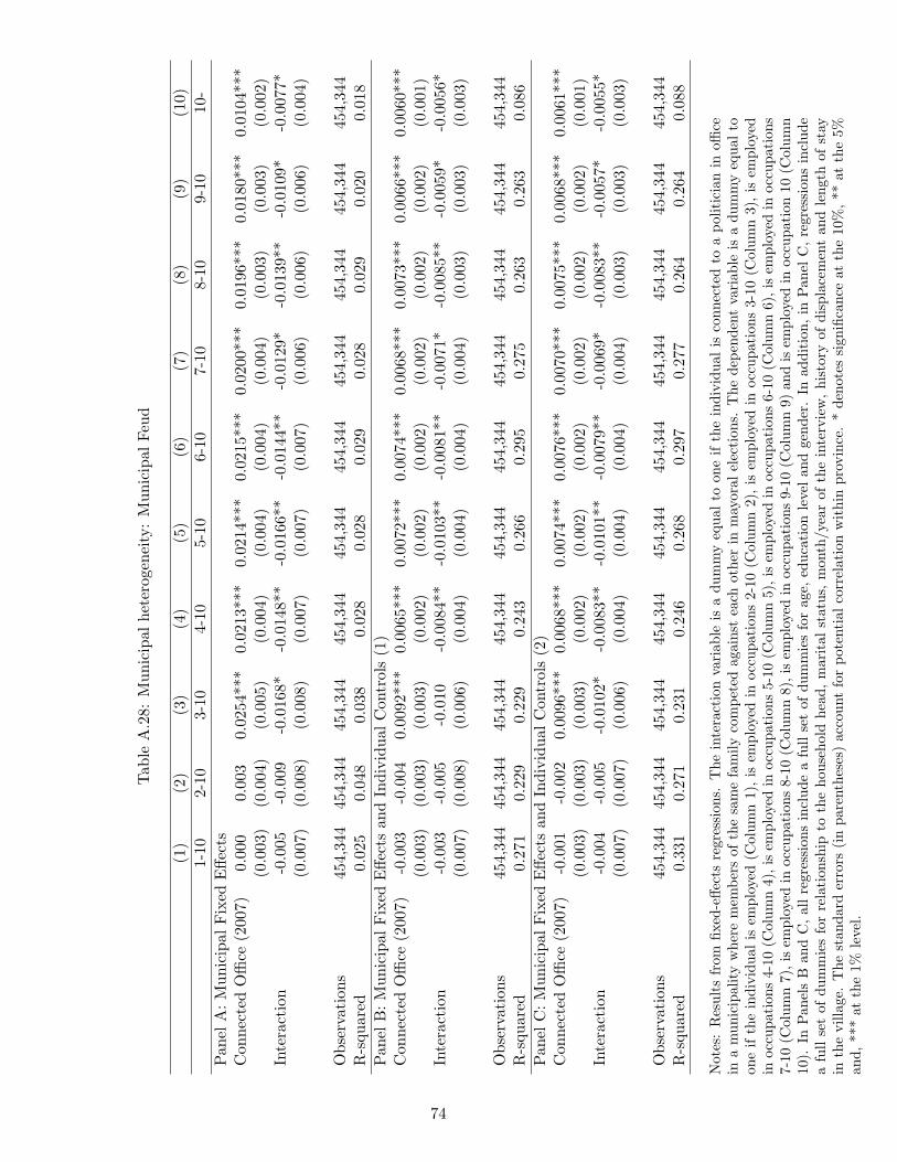
Tab

leA

.28:

Mun

icip

alhe

tero

gene

ity:

Mun

icip

alFe

ud

(1)

(2)

(3)

(4)

(5)

(6)

(7)

(8)

(9)

(10)

1-10

2-10

3-10

4-10

5-10

6-10

7-10

8-10

9-10

10-

Pan

elA

:M

unic

ipal

Fix

edE

ffect

sC

onne

cted

Offi

ce(2

007)

0.00

00.

003

0.02

54**

*0.

0213

***

0.02

14**

*0.

0215

***

0.02

00**

*0.

0196

***

0.01

80**

*0.

0104

***

(0.0

03)

(0.0

04)

(0.0

05)

(0.0

04)

(0.0

04)

(0.0

04)

(0.0

04)

(0.0

03)

(0.0

03)

(0.0

02)

Inte

ract

ion

-0.0

05-0

.009

-0.0

168*

-0.0

148*

*-0

.016

6**

-0.0

144*

*-0

.012

9*-0

.013

9**

-0.0

109*

-0.0

077*

(0.0

07)

(0.0

08)

(0.0

08)

(0.0

07)

(0.0

07)

(0.0

07)

(0.0

06)

(0.0

06)

(0.0

06)

(0.0

04)

Obs

erva

tion

s45

4,34

445

4,34

445

4,34

445

4,34

445

4,34

445

4,34

445

4,34

445

4,34

445

4,34

445

4,34

4R

-squ

ared

0.02

50.

048

0.03

80.

028

0.02

80.

029

0.02

80.

029

0.02

00.

018

Pan

elB

:M

unic

ipal

Fix

edE

ffect

san

dIn

divi

dual

Con

trol

s(1

)C

onne

cted

Offi

ce(2

007)

-0.0

03-0

.004

0.00

92**

*0.

0065

***

0.00

72**

*0.

0074

***

0.00

68**

*0.

0073

***

0.00

66**

*0.

0060

***

(0.0

03)

(0.0

03)

(0.0

03)

(0.0

02)

(0.0

02)

(0.0

02)

(0.0

02)

(0.0

02)

(0.0

02)

(0.0

01)

Inte

ract

ion

-0.0

03-0

.005

-0.0

10-0

.008

4**

-0.0

103*

*-0

.008

1**

-0.0

071*

-0.0

085*

*-0

.005

9*-0

.005

6*(0

.007

)(0

.008

)(0

.006

)(0

.004

)(0

.004

)(0

.004

)(0

.004

)(0

.003

)(0

.003

)(0

.003

)

Obs

erva

tion

s45

4,34

445

4,34

445

4,34

445

4,34

445

4,34

445

4,34

445

4,34

445

4,34

445

4,34

445

4,34

4R

-squ

ared

0.27

10.

229

0.22

90.

243

0.26

60.

295

0.27

50.

263

0.26

30.

086

Pan

elC

:M

unic

ipal

Fix

edE

ffect

san

dIn

divi

dual

Con

trol

s(2

)C

onne

cted

Offi

ce(2

007)

-0.0

01-0

.002

0.00

96**

*0.

0068

***

0.00

74**

*0.

0076

***

0.00

70**

*0.

0075

***

0.00

68**

*0.

0061

***

(0.0

03)

(0.0

03)

(0.0

03)

(0.0

02)

(0.0

02)

(0.0

02)

(0.0

02)

(0.0

02)

(0.0

02)

(0.0

01)

Inte

ract

ion

-0.0

04-0

.005

-0.0

102*

-0.0

083*

*-0

.010

1**

-0.0

079*

*-0

.006

9*-0

.008

3**

-0.0

057*

-0.0

055*

(0.0

07)

(0.0

07)

(0.0

06)

(0.0

04)

(0.0

04)

(0.0

04)

(0.0

04)

(0.0

03)

(0.0

03)

(0.0

03)

Obs

erva

tion

s45

4,34

445

4,34

445

4,34

445

4,34

445

4,34

445

4,34

445

4,34

445

4,34

445

4,34

445

4,34

4R

-squ

ared

0.33

10.

271

0.23

10.

246

0.26

80.

297

0.27

70.

264

0.26

40.

088

Not

es:

Res

ults

from

fixed

-effe

cts

regr

essi

ons.

The

inte

ract

ion

vari

able

isa

dum

my

equa

lto

one

ifth

ein

divi

dual

isco

nnec

ted

toa

polit

icia

nin

office

ina

mun

icip

alit

yw

here

mem

bers

ofth

esa

me

fam

ilyco

mpe

ted

agai

nst

each

othe

rin

may

oral

elec

tion

s.T

hede

pend

ent

vari

able

isa

dum

my

equa

lto

one

ifth

ein

divi

dual

isem

ploy

ed(C

olum

n1)

,is

empl

oyed

inoc

cupa

tion

s2-

10(C

olum

n2)

,is

empl

oyed

inoc

cupa

tion

s3-

10(C

olum

n3)

,is

empl

oyed

inoc

cupa

tion

s4-

10(C

olum

n4)

,is

empl

oyed

inoc

cupa

tion

s5-

10(C

olum

n5)

,is

empl

oyed

inoc

cupa

tion

s6-

10(C

olum

n6)

,is

empl

oyed

inoc

cupa

tion

s7-

10(C

olum

n7)

,is

empl

oyed

inoc

cupa

tion

s8-

10(C

olum

n8)

,is

empl

oyed

inoc

cupa

tion

s9-

10(C

olum

n9)

and

isem

ploy

edin

occu

pati

on10

(Col

umn

10).

InP

anel

sB

and

C,

all

regr

essi

ons

incl

ude

afu

llse

tof

dum

mie

sfo

rag

e,ed

ucat

ion

leve

lan

dge

nder

.In

addi

tion

,in

Pan

elC

,re

gres

sion

sin

clud

ea

full

set

ofdu

mm

ies

for

rela

tion

ship

toth

eho

useh

old

head

,m

arit

alst

atus

,m

onth

/yea

rof

the

inte

rvie

w,

hist

ory

ofdi

spla

cem

ent

and

leng

thof

stay

inth

evi

llage

.T

hest

anda

rder

rors

(in

pare

nthe

ses)

acco

unt

for

pote

ntia

lcor

rela

tion

wit

hin

prov

ince

.*

deno

tes

sign

ifica

nce

atth

e10

%,*

*at

the

5%an

d,**

*at

the

1%le

vel.

74