Embed Size (px)
Citation preview

1
Do Newspaper Ads Raise Voter Turnout?
Evidence from a Randomized Field Experiment
Costas Panagopoulos
Fordham University
Department of Political Science
441 E. Fordham Rd.
Bronx, NY 10458
(917) 405-9069
Jake Bowers
University of Illinois at Urbana-Champaign
Political Science and Statistics and NCSA
420 David Kinley Hall (DKH) MC-713
1407 W Gregory Dr
Urbana, IL 61801
(217) 333-3881
Acknowledgments: The authors are grateful to Tom Edmonds and to his colleagues at Edmonds Associates Inc. for support and assistance. An earlier version of this paper was presented at the Midwest Political Science Association Annual Meeting, April 2006, Chicago, IL. The authors acknowledge helpful comments from panelists and the discussant. We also thank the editors, current and former, anonymous reviewers, and Donald Green for invaluable feedback.

2
Abstract
This study describes the first randomized field experiment gauging the effects of
political advertising in newspapers. From the population of municipalities holding local
elections in 2005, we identified 4 pairs of cities that were closely matched in terms of
past voter turnout, incumbent mayoral support by the council in the previous election and
two institutional features: nonpartisan balloting and mayoral appointment by council
vote. One city in each pair was randomly assigned to receive a nonpartisan newspaper ad
that encouraged readers to vote in the 2-3 days leading up to Election Day. A
confirmatory analysis suggests newspaper advertisements likely increase voter turnout in
elections by a small amount.

3
Citizens in the United States interact more frequently and more directly with local
government than any other level of government. Local governments are responsible for
providing a vast array of services that typically include tax collection, public utilities and
education, and police and fire protection. Despite the fact that survey research indicates
Americans’ confidence in local government exceeds faith in state and federal levels, far
fewer citizens turn out to vote in local elections compared to higher-level contests. Local
elections tend to attract less than one-third of the voting-eligible electorate, and turnout
often dips below ten percent in many jurisdictions.
Several explanations have been posited to account for low voter turnout in
municipal elections. One possibility is that voters are generally pleased with their local
governments and find few incentives to participate. This is perhaps the most benign
possibility. An alternative explanation is that local elections are often lopsided contests in
which the outcome is a foregone conclusion. Voters take little interest in these pro forma
elections. A third explanation suggests municipal elections are low-salience affairs.
Lacking the intense attention and visibility of state and federal contests, voters remain
less informed and weakly mobilized to participate. Still another possibility is that turnout
in municipal elections might also be low because it is perceived that there is less at stake
or that the candidates broadly agree on what should be done.
This study examines the effects of a nonpartisan newspaper advertising campaign
designed to encourage voter participation. The central hypothesis is that a mass
communication campaign that reminds voters of the upcoming election and stresses the
importance of electoral participation raises voter turnout by providing information and

4
increasing interest and motivation. As Rosenstone and Hansen (1993: 175-176) argue,
“mobilization underwrites the costs of participation.” Accordingly, we believe that
mobilization appeals delivered via mass media communications elevate turnout by
decreasing the costs of participation in elections.
The capacity of a wide range of grassroots activities to motivate electoral
participation has been subjected to academic scrutiny by numerous studies over the past
decade. Scholars have relied increasingly on randomized field experiments to show that
techniques like door-to-door canvassing, direct mail (Gerber and Green 2000; Green and
Gerber 2008, chapters 3, 5), volunteer phone calls (Nickerson 2007b), text messaging
(Dale and Strauss 2009), street signs (Panagopoulos 2009) and Election Day festivals
(Addonazio, Green and Glaser 2007) can effectively boost turnout, while others,
including leafleting (Gerber and Green 2008), commercial and automated phone calls
(Gerber and Green 2000; Green and Gerber 2008, chapter 6) and email (Nickerson
2007a) appear to exert weak effects on turnout. Subsequent experimentation that has
investigated the socio-psychological mechanisms that underlie these effects has also
revealed that message contents may matter a great deal; appeals delivered via mail that
tap into social pressure to comply with voting norms (Gerber, Green and Larimer 2008;
Abrajano and Panagopoulos 2011; Mann 2010), express gratitude for prior voting
(Panagopoulos 2011), or that activate emotions like pride or shame (Panagopoulos 2010;
Gerber, Green and Larimer 2010) elevate turnout appreciably more than basic reminders
or civic duty messages.
Despite these insights, gleaned from over 100 randomized field experiments
conducted over the past decades, field experimental studies designed to gauge the

5
mobilizing effects of campaign communications delivered via mass media are rare. This
lacuna in the literature is understandable given the complexities and often-prohibitive
costs associated with executing real-world interventions using mass media, but
regrettable when we take into account these outlets’ capacities to reach vast audiences
and campaigns’ heavy reliance on mass media communications in actual campaigns.
Even modest treatment effects may imply that mass media advertisements may rival even
the most efficient campaign mobilization techniques.
A handful of pioneering studies have overcome these obstacles to examine the
effectiveness of mass media advertisements designed to stimulating voting. A series of
randomized field experiments using nonpartisan advertisements delivered via radio in
mayoral (Panagopoulos and Green 2008) and congressional (Panagopoulos and Green
2011) races (the latter targeted Hispanic voters) suggest radio campaigns appear to have
some positive impact on turnout. Green and Vavreck (2008) subjected cable advertising
to randomized experimentation and found evidence that such appeals motivate voting.
This experimental voter mobilization literature on mass media advertising effects
provides some guidance about the likely impact of newspaper advertisements, suggesting
the estimated bump in turnout should range between 1 and 4 percentage points on
average.
Curiously, no experimental study of which we are aware to date has investigated
the mobilization impact of newspaper advertisements. There exist over 1,600 daily
newspapers across the United States (Trent and Friedenberg 2000), and newspaper
advertisements are a popular campaign communications tactic in local elections. In a
recent study of consultants who have worked in local elections, Strachan (2003) reports

6
that 79 percent of consultants indicate their clients in local elections use newspaper
advertisements. In fact, the consultants used newspaper advertisements more frequently
than several other campaign activities in local elections including televisions
advertisements, door-to-door canvassing, literature drops and Internet sites (Strachan
2003: 25). Descriptive studies also show newspaper advertising is widespread in federal
campaigns. Herrnson (2004) reports 63 percent of all candidates for the U.S. House and
80 percent of U.S. Senate campaigns in 2002 purchased newspaper ads in local or
statewide newspapers. Despite the fact that newspaper readership has declined over the
past few decades (Paletz 1999), campaigns typically find several advantages to
newspaper advertising. A key consideration is that ad space is always available. Unlike
radio and television, which are constrained by time availability, newspapers can always
find space to display advertising (Shea and Burton 2002). Newspapers also increasingly
segment their advertising markets to permit precise targeting (Shea and Burton 2002).
Thus, studying the effects of newspapers in a systematic fashion provides important new
evidence about the effectiveness of mass communication.
This paper breaks new ground by conducting a randomized field experiment to
assess the effects of nonpartisan newspaper advertising. The central hypothesis is that a
mass communication campaign that reminds voters of the upcoming election and stresses
the importance of electoral participation raises voter turnout by providing information
and increasing interest and motivation. The experiment is based on a sample of mayoral
elections that took place in November 2005. Municipal elections have several
advantages. First, they allow us to study the effects of newspapers in campaign
environments that would naturally attract newspaper advertising when other media

7
(television or radio, for example) are often prohibitively costly or difficult to target to a
geographically compact area. Local elections, due to their low salience, are also ideal
laboratories within which to study the effects of newspaper advertising. The fact that
these elections occur in off-years, typically with little competition from other campaign
communication, makes it easier to isolate the effects of our intervention. Although the
external validity of our results remains an open question, the experiment does provide
useful information about low-salience elections in which newspaper communication
occurs in a campaign environment with few competing messages. Given the lopsided
nature of municipal elections and legislative elections at the state and federal level, the
applicability of these findings is potentially quite broad.
This paper proceeds as follows. First, we describe the procedure by which the
experimental sample was created and the way in which observations were randomly
assigned to treatment and control groups. Next, we describe the content and timing of the
newspaper campaign. We then discuss the analytic approach used to test the hypotheses
about the effects of newspaper ads on voter turnout and describe the results. We conclude
by discussing the implications of these findings and by suggesting directions for future
research.
Experimental Design
Sample construction. Of the nation’s 1,183 cities and towns with populations of
over 30,000, 281 municipalities held municipal elections in November 2005. In order to
maximize the statistical power of our experiment given our budget constraints, we sought
to create a sample of observations that, within experimental strata, were as homogeneous

8
as possible. We gathered detailed information about the institutional and political
characteristics of municipal elections these cities in order to create matched pairs. The
matching criteria included voter turnout in the previous municipal election, council
support for the incumbent mayor in the previous election (unanimous or not), whether
local elections were partisan or nonpartisan (nonpartisan) and whether or not town
councils appointed the mayor. All of the cities and towns included in the final sample
were municipalities in which the local executive is selected by council vote (as opposed
to by popular vote). Using the criteria described above, we identified 4 closely matched
pairs of cities. Once the matching exercise was completed, we randomly assigned one
city in each pair to the treatment group and the other to the control group.
Table 1 presents a list of the 4 pairs included in the final sample and provides
details about the each of the matching criterion for the corresponding localities. The
matched pair design used here in effect creates four distinct N=2 experiments, and the
models presented below analyze the data using a matched pair framework.
Did the randomization work as expected? We assess balance further in two ways:
(1) an omnibus test which compares treatment versus control differences on a number of
covariates to the differences that we would expect to observe from an ideal randomized
experiment following the same design as this one (Hansen and Bowers 2008) and (2)
some inspection of the covariate-by-covariate differences (not useful as tests per se but to
give us hints about where chance imbalances might lie in case they might make
substantively meaningful differences in our interpretation of the experiment.) (Bowers
2011).

9
The omnibus balance test reports that the configuration of our data would not be
very surprising (p=0.5) from the perspective of the hypothesis that the two groups do not
differ in any linear combination of the covariates.1 Even if the actual experiment as a
whole compares unsurprisingly with our image of a well-randomized experiment, might
one or two substantively meaningful covariates appear imbalanced? If they were, they
would not impeach the randomization procedure but might encourage closer inspection of
their relationships with treatment effects.
Figure 1 shows the differences between treated and control units on these
covariates using boxplots with scatterplots overlaid. The thick gray horizontal segments
are the means within the control and treated groups. Pairs of cities are shown using
symbols. The variables are all pair-mean centered, or pair-mean aligned, in which the
mean of the variable within the pair is subtracted from the individual city’s values. This
allows us to see all of the points on a common scale but also to preserve the meaningful
units (such as dollars or years).We see overlap in the distributions of baseline turnout,
numbers of candidates, and population within pairs. The treated and control groups
diverge rather dramatically, however, in median household income and median age. The
quantification of these individual imbalances suggests some caution in interpreting results
1 An hypothesis test compares what we observe with a distribution characterizing variation in a hypothetical world. Although large datasets justify the common use of the t-distribution (and/or Normal distribution) as the reference distribution, this study is small enough to raise concerns about the suitability of such approximations. To address this concern we never use a large sample approximation in any analysis in this paper. All of the hypothesis tests and confidence intervals reported compare what we observe to a reference distribution generated by enumerating the possible ways to re-run the experiment: that is, our experiment is small enough that we do not need to approximate, rather, we enumerate. A test that appeals to an enumerated distribution is often known as an “exact” test. See Keele, et al (2012) for an introduction to this approach for experiments in political science. See also Rosenbaum (2010, Chapter 2), for a more general introduction to randomization inference.

10
since the p-values against the null of no difference are small (p=.125 for both covariates)2
Yet, confounding only arises when a covariate is imbalanced with respect to treatment
and is also predictive of outcomes. These imbalanced covariates, do not strongly predict
vote turnout (p-values for the null hypothesis of no relationship between covariates and
turnout are .18 for median age, .48 for median household income, and .62 for percent
black).
[Figure 1 here]
The omnibus test suggested that it would not be surprising to see such a pattern
of balance and imbalance as depicted in Figure 1 from an idealized and well-randomized
study (p=.5). In fact, as a general rule, small but well run experiments may well show
such imbalances in one or more covariates. So these imbalances do not impugn the
administration of the study. We will attend to the question of how (and whether) to adjust
for selective covariate imbalance later.
Newspaper treatment. Localities in the treatment group were exposed to either
full or half-page newspaper advertisements that presented a nonpartisan get-out-the-vote
message to readers. Newspaper advertisements were printed between November 5th and
Election Day. Advertisements were professionally designed and produced by a nationally
well-established political consulting and media firm. The black-and-white ads were
printed in the local newspaper of record in each municipality. The corresponding
newspapers are indicated in Table 1.3
[Table 1 here]
2 The smallest p-value possible in this study is .0625=1/16 because there are only 16 ways to assign treatment here. The next smallest p-value is .125=2/16. 3 We combine the full and half-page treatments when we talk about comparing “treated” to “control” groups.
11
Voters in each locality were urged to vote on Election Day. Below is the text that
appeared in the advertisement. A copy of the ad is included in the Appendix.
Headline: All Politics is Local. Text: And your local government is responsible for things that affect your
everyday life. From tax assessment to police protection and clean drinking
water—it’s all part of local government. As a voter, you have the power to
make informed decisions about the candidates and the issues. Now more
than ever, your community and your country need to hear what you think.
But your opinion won’t be heard unless you vote this Election Day. Make
a difference. Vote November 8th.
Tagline: Provided as a public service by the Institution for Social and
Policy Studies and the [NAME] newspaper.
Unadjusted Test of the Strict Null Hypothesis
The first and simplest question is whether the data and design provide enough
information to render implausible a hypothesis that the treatment had absolutely no effect
on any city4. Because we have the disadvantage of a very small study but the advantage
of having randomly assigned treatment within pairs, we analyze the experimental data
using randomization-based inference. This mode of statistical inference is particularly
well-suited for small experiments because it does not require us to claim that N=8 is large
4 We acknowledge that some voters in our treatment localities may not have been exposed to our newspaper intervention, however actual rates of exposure (contact rates) to our messages are unavailable. Accordingly, we report intent-to-treat effects throughout.

12
enough to justify use of the large-sample statistical theory underlying the more common
t-test. The following analyses show that our observed data are unsurprising from the
perspective of this hypothesis (often known as the “sharp” or “strict” null hypothesis of
no effects). The observed test-statistic for the treatment effect of 1.5 percentage points is
p=.38 (using a rank-based test to account for outcomes that are overly skewed, we
estimate a treatment effect of 6 percentage points with an observed test statistic of p=.44).
Another advantage of our testing framework beyond its usefulness in small samples is
that these kinds of tests make no claims about the distribution of the outcome,
homoskedasticity, or functional form relating treatment (or covariates) to the outcome or
to each other. The treatment-versus-control differences are unsurprising from the
perspective of this null hypothesis of no effects on any city. We more or less expected
this result from the beginning: Turnout effects tend to be in the single digits in field
experiments of turnout in the United States (Green and Gerber 2008), and our sample of
cities is very small.
Even if “no effect” is unsurprising, however, we still might be interested in asking
other questions of this design and data: What kinds of turnout effects would be surprising
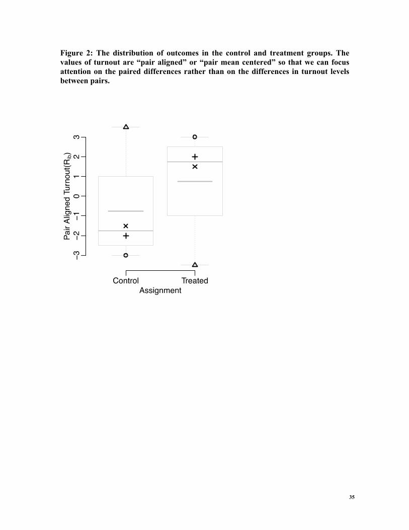
from the perspective of our data? Let us start by a simple inspection of the raw
relationship. Consider the following figure, Figure 2, where each pair has a different
symbol, the mean outcome in the two groups is depicted in a thick gray line segment and
a box plot of the distribution of outcomes in the two groups is overlaid (so that the
median is the thin gray line inside the boxes). This plot suggests that the distribution of
outcomes in the treatment group is shifted upwards compared to the outcomes in the
control group. The y-axis is in units of “proportion turning out to vote” but it is relative to
13
the mean level in the pair—so the control units tended to have lower turnout that the
mean in the pair (i.e. lower turnout than the treated units) and thus we see negative
numbers. This plot, as well as previous theory and motivation for the experiment,
recommend that we ask questions about a shift in distribution—a shift by some constant
which is the same across all cities. When we assessed hypotheses of this form
(hypotheses arising from what is often called the model of constant additive effects (Cox
1958; Rosenbaum 2010, Chap 2)), we find that the one-sided 87% confidence interval is
bounded from above by a difference of 6 percentage points of turnout. That is, we can say
that our data are fairly surprising from the perspective of hypotheses of constant additive
effects greater than 6 percentage points—where we begin to be surprised when p<.125.
The point estimates here (which are, roughly speaking, the values of the treatment effect
one would have to remove in order to align the distributions of the treated and control
groups in terms of some test statistic and are known as “Hodges-Lehmann point
estimates” (Hodges, J. and Lehmann, E. 1963; Rosenbaum 1993)) differ between the
mean-based estimate of 1.5 percentage points and the rank-based estimate of 3.25
percentage points; differences between means and medians often arise from outliers or
skewed distributions (we can that the distance between means is smaller than the
difference between medians as the differences between the corresponding horizontal lines
on that boxplot). We notice from the plot that the Battle Creek/Midland pair had a fairly
large and negative effect—this pair is a candidate for the influential point(s) that make
the rank and the mean based point-estimates. This negative turnout difference was also
very large compared to the other turnout differences in our data. So, we wonder whether
our model “fits”; that is, does it really bring the two distributions of treated and controls

14
into alignment? Figure 3 compares the results of applying the model that we just
assessed. Clearly, there is an argument for using the ranks—the middle panel shows that
units in the treatment group are brought much closer to the units in the control group if
we adjust using the difference of medians (the panel labeled “Rank HL Adjusted”)
compared to the panel in which the treated units are moved toward the controls following
the difference of means HL estimate (the panel labeled “Mean HL Adjusted”). We may
worry, however, that the Battle Creek/Midland pair is exerting undue influence on these
results or is not well fit by this simple model of treatment effects (for example when
either the medians or the means are brought closer together overall, the points
representing Battle Creek and Midland [the triangles] move farther apart: showing that
the hypotheses are not doing a good job of explaining that one pair); we return to this
concern below.
[Figures 2, 3 here]
Overall, the model of constant treatment effects implies a shift in distribution
between treated and control units. Our data are surprising from the perspective of this
model when the size of the shift is 6 percentage points of turnout or more. Yet, we have
lingering concerns that perhaps this simple model is not as substantively interesting as a
model in which the treatment backfires in at least some cities. We proceed with analyses
to take this into account.
Identify Surprising Effects: Attributable Effects

15
In our initial analyses above, we essentially ignored the pattern shown in Figures
2 and 3 in which three treatment cities displayed higher turnout than the corresponding
control cities and one pair in which the pattern reversed and was stronger than any other
within-pair difference. Also, the model of effects that we assessed involved the same
treatment effect for every pair, yet, close inspection of Figure 2 shows the pairs with
lower turnout in control cities seemed to have larger differences than pairs with higher
turnout. So, we have two reasons to ask questions about effects that go beyond the
models of constant additive effects: either we might want to know how plausible it would
be for treatment to be largely positive but rarely (yet dramatically) negative and/or we
might wonder whether there is some relationship with baseline turnout and the
intervention The previous questions could have been formalized as saying that potential
outcomes in response to treatment, yZ=1, i ≡ y1,i are exactly the same as potential outcomes
in response to control, y0i, or H0 : y1i = y0i. Our assessment of the idea that turnout might
increase by the same amount in every city in treatment could have been written H0:y1i =
y0i + τ. Of course, we are not restricted to these questions, and a kind of question that
suggests itself in this case, in which we have two non-constant patterns of response to
treatment, is H0: y1i = y0i + τi — i.e. each unit has its own additive treatment effect. With
this model we can ask questions about both collections of τi or, perhaps more usefully, we
can ask questions about aggregates of τi. In particular, we might wonder about the sum of
the within-treated unit effects, A = Σni=1 τi —the total number of turnout percentage points
increased by the treatment across all cities in the study. Rosenbaum (2001, 2002) called
this estimand an “attributable effect” and developed it in the context of binary outcomes
where τi was restricted to be either 0 or 1. Hansen and Bowers (2009) applied this model
16
to the case of few strata and clustered treatment assignment in a study of binary vote
turnout. Here we extend the method to encompass outcomes that are not binary but are
counts. That is, we can think of A as “total percentage points of turnout caused by the
treatment across all cities”: this estimate summarizes the various τi, where now we let τi
be an integer rather than the 0 or 1 as used in previous work. This simplifies the outcome
variable somewhat (from a real, decimal, number to an integer) but in a study of this size
the loss of measurement precision is not substantively meaningful.
Recasting our questions in this way implies that, for a given hypothesized A0 (say,
A = 1), we can list all of the ways that a vector of τ={τ1 τ2 τ3 τ4} can be summed to that
number. If all of the elements of τ are nonnegative, we can list the partitions of the
integer A0 and evaluate how surprising our data would look from that perspective for each
partition. (We do not strictly use partitions, however, since we want to allow at least one
set to have negative numbers. For an introduction to partitions see Niven (1965, Chapter
6). Consider the case of A=0; if we allow negative effects, one can show that there are
6181 ways for four integers, each having values between -10 and 10, to add up to 0. If we
reject all of those “atomic hypotheses” (i.e. hypotheses that differ in the details about
which treated unit receives which amount of treatment effect but which all sum to 0),
then we can reject H0: A0=0. If we cannot reject at least one of them, then we say that we
cannot reject A0=0. On a dataset this small, and with reasonable substantive limits on the
unit level hypotheses of interest, we can directly test all of the atomic hypotheses implied
by a substantively interesting range of A conditional on a limited set of individual level τi
(that is, there are an infinite number of ways positive and negative integers can sum to 0,
but there are only a finite number of ways the integers between -10 and 10 can do so and

17
we are willing to only entertain hypotheses in which the treatment increased turnout by
less than 10 points, or decreased turnout by no more than 10 points).5 Figure 4 shows
both ranges of two-sided p-values for the atomic hypotheses associated with a given
composite hypothesis (defining the x-axis). We switch to considering two-tailed tests
here because we are considering both positive and negative null hypotheses about A and
τi in this bit of exploratory analysis following the discovery that the treated-control
difference between Battle Creek and Midland was strongly negative.
[Figure 4 here]
What does it mean that hypotheses about A make our data surprising when A is
more than 36 percentage points of turnout? Since we considered hypotheses in which
turnout in the control groups decreased, we focus here on the two-sided interval, looking
more closely at two hypotheses: H0 : A0 = 36 and H0 : A0 = 37. We find that different
collections of hypotheses about 7, 8, 9, and 10 percentage points of turnout are all
equally unsupported by our data at the α = .125 level. The largest, total amount of turnout
in which at least one atomic hypothesis was not rejected at α=.125 was 36 (and, in this
case, it was only one atomic hypothesis with a p=.25 which causes us to not-reject A0=36
and thus leave it inside the confidence interval). In Rosenbaum’s attributable effects
framework, we only attribute one point of turnout to each unit, so we could merely divide
36 by the number of treated units to conclude that the upper-bound on a two-sided 87%
confidence interval for the number of percentage points of turnout attributable to the
treatment is 36/4 ≈ 9 percentage points: Nine percentage points per treated city is the
average atomic hypothesis for A=36. Although this approach is reasonable, it was built
5 A replication archive containing all of the data and syntax files used to produce the analyses we report in this study is available at: [TBD]
18
for binary outcomes: our outcomes (which we are treating as a count of percentage
points) offer us more information about the outcomes for each unit. For example, we also
see that the hypotheses which sum to 36 (and which obey our restrictions on τi) involve τi
which are never less than 6. In our analysis, in fact, we never observe more than one
treated city with τi=6 where A=36. Notice also that the attributable effects includes nested
within it the constant effects hypothesis:{-7 – 6} bound the two-sided 87% confidence
interval for τ in that model). That is, when we assess the constant effects hypotheses, we
also learn something about the unit-specific hypotheses that we assess here. So, there are
a couple of obvious ways to translate the 36 percentage points of turnout finding from the
aggregate to the units. We could argue, as we do above, that the 36 percentage points
finding can be understood as about 9 percentage points on average. However, because
our outcome is not binary, in principle, we can know more about the specific hypotheses
which were more or less supported by our data when A0 = 36 than might be revealed by
an average. For example, we might focus attention on the atomic hypotheses which
summed to 36 but which were most supported by the data (which made the data least
surprising). The largest, but least surprising hypotheses about the effects of this
intervention summed to 36 points of turnout across the four cities, but among atomic
hypotheses adding up to 36, the least surprising one allocated 6 percentage points to the
treatment effect in the first pair (where Sioux City was treated) and 10 percentage points
to the treatment effect in the other pairs.
Finally, let us consider the hypotheses about A that made the data surprising, but
for A0 which we could not reject from the confidence interval because at least one of the
atomic hypotheses contained within it could not be rejected. In Figure 4 we see this

19
interval at the center of the plot: from about 3 percentage points of turnout to about 9
points of turnout no atomic hypothesis was incompatible with the data, but hypotheses
begin to make our data surprising for A greater than 9 and less than 3.
There are two kinds of questions that we can address with this analysis: (1) which
hypotheses about A and τ make our data look very strange (and thus are worthy of
rejection from an interval of plausible values) and (2) which hypotheses make our data
look least surprising. It is clear that our data look unsurprising from the perspective of
hypotheses about A from 3 to 9: no atomic hypothesis in that range received a p-value
less than .25. The mean atomic hypothesis in this central, not-rejectable, range was about
1.5 percentage points per unit. Or, we can say that even among the most surprising
hypotheses about A=4, 5 or 6 total points of turnout, the mean atomic hypotheses were
unequal—2.5 points for the first pair, about 0 points for the second pair, 2 and 1.6 points
for the third and fourth pairs respectively. Recall that second pair was Battle
Creek/Midland where the treatment-minus-control difference was -7 points of turnout.
The attributable effects approach has the benefit of allowing us to ask questions about
effects defined for each unit. In a study like this one, we have the luxury of actually
canvassing these hypotheses. The costs of the approach are computational (we tested
194,481 hypotheses in about five minutes) and, more importantly, conceptual: how
should we summarize the results of such an analysis? We have tried to go back and forth
between talking directly about total percentage points of turnout and unit level summaries
such as means of the unit-level effects which add up to the totals. We cannot exclude the
idea that this study had no effects at all. Yet the hypotheses that are least surprising do

20
not include 0 total points of turnout but rather are centered around 3 to 9 total percentage
points of turnout distributed unequally across the 4 cities treated in this study.
An Exploratory Epilogue
We now consider an additional, intriguing possibility, largely by way of a
supplemental, exploratory analysis spurred by the suggestion that the intervention had a
negative effect in Midland. What if we could exclude the Midland/Battle Creek pair from
our analysis? This pair of cities in Michigan had the lowest turnout in elections held
before the intervention of all the cities included in the study (turnout in the elections held
prior to 2005 was 12 and 13 percent for Battle Creek and Midland respectively). We do
not have adequate qualitative information to discuss the mechanisms by which a
treatment intervention in a low-turnout city may backfire. Imagine, however, that a some
hidden moderator causes interventions to increase turnout in most units but decreases
turnout in others. Since we only have one pair where we observe a negative effect, we
cannot split the data into two subgroups to analyze the negative versus positive effects
pairs. Instead we exclude the Midland/Battle Creek pair and analyze the remaining
subgroup (the three pairs in which we saw no dramatic downward shifts in turnout).
When we restrict attention to the positive pairs (going from N=8 to N=6), we find,
surprisingly, that the null of no effects is no longer so plausible (p=.125). In this case, the
data would be surprising from the perspective of the hypothesis—as surprising as
possible with only 6 units in 3 pairs since p-values less than .125 are not possible with
only 8 possible ways to assign treatment in 3 pairs. We observe that a gain in

21
homogeneity on outcomes more than makes up for the loss in sample size. The 75%
confidence interval for the constant effects hypotheses now ranges from 3 to 6 (compared
to -7 to 6 when we consider all 8 cities).
Next we turn to considering attributable effects. Recall that the composite
hypothesis is rejected only if all of the atomic hypotheses under it are rejected. We use
α=.25 since the minimum p=.125 and thus a two-tailed hypothesis test has minimum
p=.125*2= .25. The total effect that is largest but still not inconsistent with our data
(α=.25) is A=26 (from two-tailed tests) and thus the average effect per unit would be
about 26/4 = 6.5 percentage points of turnout. Figure 5 shows this shift in the areas of
surprise/plausibility. In this figure, we see that all A from 12 to 14 are equally
unsurprising (where all atomic hypotheses cannot be rejected; p=1 for all). And the
hypothesis that the same effects hold across units is less difficult to maintain: A=12 or
τ=4 would be the most difficult hypothesis about constant effects to reject (p=1) and we
see the constant effects confidence interval for A ranging from 9 to 18 or for τ from 3 to
9.
[Figure 5 here]
Midland and Battle Creek, Michigan, are a very interesting pair of cities. They
had extremely low turnout before the experiment was conducted and showed a kind of
perverse turnout pattern after the intervention. By excluding this pair, we gain much more
precision to answer questions about positive treatment effects. If we had more than one
such pair, we may worry about why our treatment backfired or had harmful effects for
some cities. With this design we are left with a tantalizing piece of evidence that is not
entirely incompatible with that from other studies also showing that turnout interventions

22
matter much more for some voters than for others (Berinsky, Burns, and Traugott (2001);
Berinsky (2005); Hansen and Bowers (2009)).
Summary
Did the newspaper advertisement intervention have an effect? We can never
answer such a question directly. Rather, we can talk about “the probability of an effect”
in the Bayesian framework or “the probability of an effect given a hypothesis” in the
frequentist framework. Since this study was randomized and was small, we have worked
here within the frequentist framework, and especially with some extensions of the
framework that can be linked back to the pioneering work on the invention of randomized
experiments by R.A. Fisher (1935) and recent extensions and developments by P.
Rosenbaum. Fisher would change the question about effects to a question comparing a
hypothesis to an observed value: “If the intervention had no effect, how surprising would
it be to observe what we do observe?” In answer to this question, we have to say that it
would not be very surprising to see the kinds of turnout differences extant in the current
study under Fisher’s sharp null. Yet we also can say that this result is very sensitive to the
presence of one pair of cities which showed a large and negative post-treatment
difference in turnout. What kinds of hypotheses about effects can we exclude as overly
surprising based on these data? Our best answer allows each treated city to have its own
effects. No more than 28 total points of turnout are compatible with our data (which
amounts to about 7 points per unit). We can narrow this upper interval and exclude the
hypothesis of no effects by excluding the pair showing an aberrant and large negative

23
effect. If, in some rare circumstances, newspaper advertisements would depress turnout
and in most others it would increase it, then we could say that our study shows evidence
of a small positive effect of turnout (on those cities which, for reasons beyond the scope
of this paper, are in the majority). If we are likely to see large chance variations in
treatment assignment (where the underlying mechanism is the same across all cities but,
by chance, turnout in some treated cities is observed lower than turnout in control cities),
then we cannot claim to have observed a treatment effect which is distinguishable from
zero in this small study. So we are left wondering about whether backfiring turnout
interventions would be systematically observed for some types of cities in larger studies
and about the possible mechanisms for such effects or whether we merely have a chance
aberration in this one deployment of a newspaper advertisements experiment.
Evaluating Cost-Effectiveness
We acknowledge that our point estimates for treatment effects range widely and
are associated with considerable uncertainty. Even so, what could we glean about the
probable cost-effectiveness of newspaper advertising as a means of increasing voter
turnout? If we suppose that one newspaper ad increases turnout by 1.5 percentage points
(the observed difference in mean turnout between our treatment and control cities), this
would suggest newspaper advertising may be competitive with other get-out-the-vote
tactics in terms of cost-effectiveness. The average city in our sample has a population of
60,000, of whom approximately 70% are eligible to vote. Approximately 75% of voting
eligible citizens are registered to vote, which means that an average city has 31,500

24
registered voters. Raising turnout among registered voters by 1.5 percentage points in an
average city implies an increase of 473 votes. On the cost side of the equation, purchase
of a half page of newspaper advertising is an average expenditure of $2,500 per city.
Paying $2,500 to produce 473 votes—at just about $5 per vote—is a bargain, putting
nonpartisan newspaper advertisements on par with radio advertisements in terms of cost
effectiveness (Panagopoulos and Green 2008; 2011) and rendering them somewhat more
cost effective than advertisements shown on cable television (estimated to produce votes
at a rate of $15 per vote) (Green and Gerber 2008: 132-133; Green and Vavreck 2008).
The typical nonpartisan, direct mail campaign generates votes at more than $60 per vote;
commercial phone banks often produce votes are rates of $30-90 per vote (Green and
Gerber 2008, chapter 6; Nickerson 2007b; Arceneaux, Gerber and Green 2006). Even
relatively efficient grassroots methods, such as door-to-door canvassing or high-quality
volunteer phone banks, can produce votes at a rate of $20 per vote (Green and Gerber
2008, chapter 3; Nickerson 2007b).
Conclusion
As the first field experiment to examine the mobilization effects of political
advertising in print media, this study offers a number of methodological and substantive
insights. In terms of the methodology of design, this experiment demonstrates the
feasibility of studying newspapers’ effects using random assignment in real-world
settings. The research paradigm used here is a systematic and reproducible method that

25
can be applied to further research on print media and other forms of mass
communication.
To date, field experiments on the effects of the mass media advertising are still
rare, but they are growing in number. Randomized mass media interventions have been
deployed to shed light on how television (Green and Vavreck 2008) and radio
advertisements (Panagopoulos and Green 2008; 2011) influence voting behavior. Some
of the advantages of such interventions include the fact that subjects are exposed to these
messages in naturalistic environments, absorbing messages in the same way that they
would under ordinary conditions. Furthermore, outcomes are measured in an unobtrusive
and externally valid manner. Given random assignment, causal inference can be
generated reliably.
This initial foray into investigating the impact of newspaper advertisements on
electoral participation using field experimental techniques reveals some promising
findings and provides a guidepost for further research. To begin with, subsequent studies
would allow us to expand the power of the current project significantly. Since this is the
first study to evaluate the impact of newspaper advertisements on electoral behavior,
power calculations were difficult given that there was no existing baseline for year-to-
year variability in rates of participation.
The current study also reflects a limited exploration of the full power of
newspapers as a medium. Budgetary constraints, for example, restricted us to running
only one ad in each locality. An expanded study would allow us to procure more
comprehensive coverage in the treatment markets, expanding the overall reach and
frequency of exposure to the newspaper messages. Relative ease in ad production also

26
makes it possible to vary message content in future experiments. Voters in the current
study, for example, were exposed exclusively to nonpartisan get-out-the-vote messages.
Additional research would allow us to investigate how the results may (or may not)
change if the appeal is partisan in nature, although recent work suggests differences
between partisan and nonpartisan appeals may be minimal (Panagopoulos 2009).
Additional extensions of this research can evaluate the degree to which newspaper
advertising decisions can influence editorial coverage of the campaign or endorsements
in local newspapers.
Despite the limitations we acknowledge, the findings of this study suggest
newspaper advertising can play a role in increasing voter turnout. The analyses we
conduct and describe above present the first direct evidence derived from a field
experimental study of newspaper advertisements. Moreover, we argue that the field
experimental methodology using a matched pairs design is a productive way to measure
the effects of newspaper advertising on political behavior and can help place the findings
of observational studies into perspective.

27
References
Abrajano, Marisa and Costas Panagopoulos. 2011. “Does Language Matter: The Impact
of Spanish Versus English-Language GOTV Efforts on Latino Turnout.”
American Politics Research 39 (94): 643-663.
Addonizio, Elizabeth, Donald Green, and James M. Glaser. 2007. “Putting the Party
Back into Politics: An Experiment Testing Whether Election Day Festivals
Increase Voter Turnout.” PS: Political Science & Politics. 40: 721-727.
Arceneaux, Kevin, Alan S. Gerber, and Donald P. Green. 2006. ‘‘Comparing
Experimental and Matching Methods using a Large-scale Voter Mobilization
Experiment.’’ Political Analysis 14 (Winter): 37-62.
Atkin, C. and G. Heald. 1976. “Effects of Political Advertising.” Public Opinion
Quarterly 40: 216-228.
Bartels, Lawrence. 1993. “Messages Received: The Political Impact of Media Exposure.”
American Political Science Review (87) June: 267-285.
Berelson, Bernard R., Paul Lazarsfeld and William McPhee. 1954. Voting. Chicago:
University of Chicago Press.
Berinsky, Adam. 2005. “The Perverse Consequences of Electoral Reform in the United
States.” American Politics Research 33(4): 471–491.
Berinsky, Adam J., Nancy Burns, and Michael W. Traugott. 2001. “Who Votes by Mail?
A Dynamic Model of the Individual-Level Consequences of Voting-by-Mail.”
Public Opinion Quarterly 65: 178–197.

28
Bowers, Jake. 2011. “Making Effects Manifest in Randomized Experiments.” In
Druckman, J. N., Green, D. P., Kuklinski, J. H., and Lupia, A., eds., Cambridge
Handbook of Experimental Political Science. New York: Cambridge University
Press.
Bowers, Jake, and Costas Panagopoulos. 2011. “Fisher’s Randomization Mode of
Statistical Inference, Then and Now.” Working Paper, University of Illinois at
Champaign-Urbana.
Cardy, Emily A. 2005. “An Experimental Field Study of the GOTV and Persuasion
Effects of Partisan Direct Mail and Phone Calls.” Annals of the American
Academy of Political and Social Science 601: 28-40.
Cox, David R. 1958, The Planning of Experiments. New York: John Wiley. Dale, Allison and Aaron Strauss. 2009. “Don’t Forget to Vote: Text Message Reminders
as a Mobilization Tool.” American Journal of Political Science 54 (4): 787-804.
Erikson, Robert. 1976. “The Influence of Newspaper Endorsements in Presidential
Elections: The Case of 1964.” American Journal of Political Science 20: 207-233.
Fisher, R.A. 1935. The Design of Experiments. Edinburgh: Oliver and Boyd.
Franz, Michael M. and Travis Ridout. 2007. “Does Political Advertising Persuade?”
Political Behavior 29 (4): 465-492.
Gerber, Alan and Donald P. Green. 2000. “The Effects of Canvassing, Telephone Calls,
and Direct Mail on Voter Turnout: A Field Experiment.” American Political
Science Review 94(3): 653-663.

29
Green, Donald P., and Alan S. Gerber. 2008. Get out the Vote!: How to Increase Voter
Turnout. 2nd edition. Washington, D.C.: Brookings Institution Press.
Gerber, Alan S., Donald P. Green, and Christopher W. Larimer. 2008. “Social Pressure and
Voter Turnout: Evidence from a Large Scale Field Experiment.” American Political
Science Review 102 (February): 33-48.
______. (2010). “An Experiment Testing the Relative Effectiveness of Encouraging
Voter Participation by Inducing Feelings of Pride or Shame.” Political Behavior
32 (3): 409-422.
Green, Donald and Lynn Vavreck. 2008. “Analysis of Cluster-Randomized Experiments:
A Comparison of Alternative Estimation Approaches.” Political Analysis 16: 138-
152.
Hansen, B.B., and J. Bowers. 2008. “Covariate Balance in Simple, Stratified and
Clustered Comparative Studies.” Statistical Science 23: 219-41.
Hansen, B. B., and J. Bowers. 2009. “Attributing Effects to A Cluster Randomized Get-
Out-The-Vote Campaign.” Journal of the American Statistical Association 104
(Septemer): 873—885.
Harris, Phil, A. Lock and J. Roberts. 1999. “Limitations of Political Marketing?” In
Newman, Bruce. Handbook of Political Marketing. Thousand Oaks: Sage.
Herrnson, Paul S. 2004. Congressional Elections: Campaigning at Home and in
Washington: CQ Press. 4th edition.
Hodges, J. L.; Lehmann, E. L. 1963. “Estimation of Location Based on Ranks.” Annals of
Mathematical Statistics 34 (2): 598–611.
30
Huber, Gregory and Kevin Arceneaux. 2007. “Identifying the Persuasive Effects of
Presidential Advertising.” American Journal of Political Science 4: 957-977.
Iyengar, Shanto and Donald Kinder. 1987. News that Matters. Chicago: Chicago
University Press.
Kaid, L. 1976. “Measures of Political Advertising.” Journal of Advertising Research
16(5): 49-53.
Keele, Luke, McConnaughy, Corrine, and White, Ishmail. 2012, “Strengthening the
Experimenters Toolbox: Statistical Estimation of Internal Validity,” American
Journal of Political Science. (forthcoming).
Lazarsfeld, Pail, Bernard Berelson and Hazel Gaudet. 1948. The People’s Choice. New
York: Columbia University Press.
Mann, Christopher B. 2010. “Is There Backlash to Social Pressure? A Large-Scale
Field Experiment on Voter Mobilization.” Political Behavior 32 (3): 387-408.
McCleneghan, J. Sean. 1987. “Impact of Radio Ads on New Mexico Mayoral Races.”
Journalism Quarterly 64: 590-593.
Miron, Dorina. 1999. “Grabbing the Nonvoter.” In Newman, Bruce. Handbook of
Political Marketing. Thousand Oaks: Sage.
Nickerson, David. 2007a. “The Ineffectiveness of E-vites to Democracy: Field
Experiments Testing the Role of E-Mail on Voter Turnout.” Social Science
Computer Review 25 (4): 494-503.
______. 2007b. “Quality is Job One: Volunteer and Professional Phone Calls,” American
Journal of Political Science 51(2):269-282.

31
Niven, I.M. 1965 Mathematics of Choice: Or, How to Count without Counting. New
York: Random House.
Palda, K. 1973. “Does Advertising Influence Votes? An Analysis of the 1966 and 1970
Quebec Elections.” Canadian Journal of Political Science 6: 636-655.
Paletz, David. 1999. The Media in American Politics: Contents and Consequences. New
York: Longman.
Panagopoulos, Costas. 2011. “Thank You for Voting: Gratitude Expression and Voter
Mobilization.” Journal of Politics 73 (3): 707-717.
______2009. “Street Fight: The Impact of a Street Sign Campaign on Voter Turnout.”
Electoral Studies 28: 309-313.
______.(2010). “Affect, Social Pressure and Prosocial Motivation: Field Experimental
Evidence of the Mobilizing Effects of Pride, Shame and Publicizing Voting
Behavior.” Political Behavior, 32 (3): 369-386.
Panagopoulos, Costas, and Donald P. Green. 2008. “Field Experiments Testing the
Impact of Radio Advertisements on Electoral Competition.” American Journal of
Political Science 52 (1): 156-168.
______. 2009. “Partisan and Nonpartisan Message Content and Voter Mobilization.”
Political Research Quarterly 62(1): 70-76.
______. 2011 “Spanish-Language Radio Advertisements and Latino Voter Turnout in the
2006 Congressional Elections: Field Experimental Evidence.” Political Research
Quarterly 64 (3): 588-599.

32
Patterson, Thomas and R. McClure. 1976. The Myth of Television Power in National
Politics. New York: Putnam.
Rosenbaum, Paul R. 2001. “Effects Attributable to Treatment: Inference in Experiments
and Observational Studies with a Discrete Pivot.” Biometrika 88(1): 219–231.
______. 2002. Attributing Effects to Treatment in Matched Observational Studies.
Journal of the American Statistical Association 97 (March)): 183–192.
______. 1993. “Hodges-Lehmann Point Estimates of Treatment Effects in Observational
Studies.” Journal of the American Statistical Association 88: 1250-1253.
______. 2010. Design of Observational Studies. New York: Springer
Strachan, Cherie J. 2003. High-Tech Grass Roots: The Professionalization of Local
Elections. Lanham: Rowman and Littlefield.
Thorson, Esther. 2005. “Mobilizing Citizen Participation.” In Geneva Overholser and
Kathleen Hall Jamieson, eds. The Press. New York: Oxford University Press.
Wring, Dominic. 1999. “The Marketing Colonization of Political Campaigning.” In
Newman, Bruce. Handbook of Political Marketing. Thousand Oaks: Sage.
Zaller, John. 1996. “The Myth of Massive Media Impact Revived: New Support for a
Discredited Idea.” In Political Persuasion and Attitude Change, ed. Diana Mutz,
Paul Sniderman and Richard Brody. Ann Arbor: University of Michigan Press.
Zhang, Zhengyou. 1996. Parameter Estimation Techniques: A Tutorial with Application
to Conic Fitting. Computer Based Learning Unit: University of Leeds.
Zou, H. 2006. “The Adaptive Lasso and Its Oracle Properties.” Journal of the American
Statistical Association 101 (476): 1418–1429.

33
Table 1: Experimental Sample (Treatment and Control Groups)
Pair Code Treatment (T)
State
City
Newspaper Turnout (t-1)
1 C MI Saginaw 17
1 T IA Sioux City Sioux City Journal 21
2 C MI Battle Creek 13
2 T MI Midland Midland Daily News 12
3 C OH Oxford 26
3 T MA Lowell Lowell Sun 25
4 C WA Yakima 48
4 T WA Richland Tri-City Herald 41

34
Figure 1: Differences between treated and control units on baseline covariates of using boxplots with scatterplots overlaid. The thick gray horizontal segments are the means within the control and treated groups. Thin lines in the middle of the boxes are medians. Pairs of cities are shown using symbols. The variables are all pair-mean centered.
35
Figure 2: The distribution of outcomes in the control and treatment groups. The values of turnout are “pair aligned” or “pair mean centered” so that we can focus attention on the paired differences rather than on the differences in turnout levels between pairs.

36
Figure 3: The unadjusted comparison of controls versus treated (left most plot) as compared to the results of adjusting the treatment group based on the Hodges-Lehmann (HL) point estimates derived from two different test statistics (Wilcoxon paired signed ranks and the mean difference). Notice that the control group remains the same and it is the hypotheses which imply changes in the distribution of the treatment group compared to the unadjusted, observed, outcomes.

37
Figure 4: Box-plots of two-tailed p-values for tests of total turnout effects (sums of unit-specific additive turnout effects). The limits of the two-sided 87% confidence intervals are show in pink. The dashed horizontal line at p = (1 − .87) shows the dividing line for exclusion of A from the interval. The circles show the means of the p-values.
−40 −34 −28 −22 −16 −10 −4 0 4 8 12 17 22 27 32 37
0.2
0.4
0.6
0.8
1.0
A
p

38
Figure 5: Box-plots of two-tailed p-values for tests of total turnout effects (sums of unit-specific additive turnout effects) after removing Battle Creek and Midland. The limits of the two-sided 87% confidence intervals are show in pink. The dashed horizontal line at p = (1 − .87) shows the dividing line for exclusion of A from the interval. The circles show the means of the p-values.
−30 −25 −20 −15 −10 −6 −2 1 4 7 10 14 18 22 26 30
0.4
0.6
0.8
1.0
A
p

39
Appendix: Newspaper Ad


