Policy Research Working Paper 6034

Do Migrants Really Foster Trade?

The Trade-Migration Nexus, a Panel Approach 1960–2000

Christopher R. Parsons

The World BankDevelopment Research GroupTrade and Integration TeamApril 2012

WPS6034P

ublic

Dis

clos

ure

Aut

horiz

edP

ublic

Dis

clos

ure

Aut

horiz

edP

ublic

Dis

clos

ure

Aut

horiz

edP

ublic

Dis

clos

ure

Aut

horiz

ed

Produced by the Research Support Team

Abstract

The Policy Research Working Paper Series disseminates the findings of work in progress to encourage the exchange of ideas about development issues. An objective of the series is to get the findings out quickly, even if the presentations are less than fully polished. The papers carry the names of the authors and should be cited accordingly. The findings, interpretations, and conclusions expressed in this paper are entirely those of the authors. They do not necessarily represent the views of the International Bank for Reconstruction and Development/World Bank and its affiliated organizations, or those of the Executive Directors of the World Bank or the governments they represent.

Policy Research Working Paper 6034

Despite the burgeoning empirical literature providing evidence of a strong and robust positive correlation between trade and migration, doubts persist as to unobserved factors which may be driving this relationship. This paper re-examines the trade-migration nexus using a panel spanning several decades, which comprises the majority of world trade and migration in every decade. First the findings common to the literature are reproduced. Country-pair fixed effects are then used to account for unobserved bilateral factors, the implementation of which removes all of the positive impact of migration on trade. In other words the unobserved factors, a leading candidate for which

This paper is a product of the Trade and Integration Team, Development Research Group. It is part of a larger effort by the World Bank to provide open access to its research and make a contribution to development policy discussions around the world. Policy Research Working Papers are also posted on the Web at http://econ.worldbank.org. The author may be contacted at cparsons@worldbank.org or lexcrp1@nottingham.ac.uk. 

it is argued is international bilateral ties, are on average strongly and positively correlated with migrant networks. Dividing the world into the relatively affluent North and poorer South, the results show that migrants from either region only affect Northern exports to the South. This is intuitive since in general countries of the North export more differentiated products and information barriers between these regions are greatest. A country-level analysis further shows that migrants may both create and divert trade. Taken as a whole, the results demonstrate the large biases inherent in cross-sectional studies investigating the trade-migration nexus and highlight the extent to which previous results have been overstated.

Do Migrants Really Foster Trade?

The Trade-Migration Nexus, a Panel Approach 1960-2000

Christopher R. Parsons1

Key Words: International Trade, Panel Data, Immigration, Emigration

JEL Codes: [F22], [015], [J11], [F16]

1The Leverhulme Centre for Research on Globalisation and Economic Policy (GEP). The correspondence address is: Nottingham

School of Economics, Clive Granger building, University Park, Nottingham, NG7 2RD, United Kingdom. Christopher Parsons

may be contacted by e-mail at lexcrp1@nottingham.ac.uk, by phone on: +44 (0)1159 951 5620 or by fax: +44 (0)1159 951 4159.

The author gratefully acknowledges funding from the Economic and Social Research Council and support from the World Bank

Knowledge for Change Program.. He is appreciative to Alison Ma for the clarifications received with regards the trade data and also

wishes to thank James Anderson, Michel Beine, Richard Disney, Gabriel Felbermayr, Richard Kneller, Çağlar Özden, Maurice

Schiff and Richard Upward for very useful and timely comments.

2

1. Introduction

Germany and Turkey have been in contact with one another, since at least the attempted expansion of the

Ottoman Empire north of the Balkans, which culminated in the second siege of Vienna in 1683. Official

diplomatic relations were marked however by the opening of the Berlin embassy in Constantinople in the

18th century, which led to increased labor mobility between the two cities and numerous subsequent trade

agreements. In 2000, Germany remained the most important trading partner for Turkey, while Turkey

represented the 17th most important trading partner for Germany - which at the time was the largest

exporting nation in the world. Perhaps the most famous use of early migrant labor between the two

nations was the joint imperial endeavor of constructing the Baghdad railway in the lead up to the Great

War, “which was instrumental in forging a lasting Turco-German relationship” (McMurray 2001). Large

numbers of Turkish workers began arriving in Germany in the 1960s however, to meet labor shortfalls

exacerbated by the construction of the Berlin wall, which deprived West Germany of relatively cheap

labor from the East. In 2000, the Turks in Germany represented the single largest diaspora in Europe and

indeed the second largest South-North migration corridor in the world.2 Similarly, the numbers of

Germans in Turkey - most of which are ethnic Turks - is the second largest North-South corridor globally

(Özden et al 2011).3

The Turkish-German case is a good example of an idiosyncratic international bilateral tie that is difficult

to account for empirically. Such ties are underpinned by a complex combination of historical, political

and cultural characteristics, which in turn are both the cause and the consequence of myriad past events.

Although gravity models investigating the trade-migration nexus typically uncover a robust and positive

relationship between these two forces of globalization, there clearly exists unobserved heterogeneity,

which is not captured by standard gravity variables - as exemplified by the Turkish-German – which

might be driving this relationship. Leading scholars also call into question the robustness of previous

findings. Hanson (2007), for example, states “it is difficult to draw causal inferences from these results,

since immigration may be correlated with unobserved factors that affect trade, such as trading partners’

cultural similarity or bilateral economic policies” (pg. 43). Similarly Lucas (2006) is also sceptical since

“…reservations persist as to the potential for other, unobserved phenomena to be stimulating both trade

and migration. ……Overall the estimated effects seem improbably large, though perhaps indicative of a

very real underlying phenomenon” (pg. 212).

This paper is the first to investigate the links between trade and migration in a panel spanning several

decades, 1960-2000, which comprises the majority of world trade and migration in each period. The panel

2 The largest South-North corridor is the Mexicans in the United States. 3 The largest North-South corridor is the Americans in Mexico.

3

facilitates the implementation of time-varying country fixed effects to control for the common omission

of multilateral resistance terms and, crucially, also for country-pair dummies to control for unobserved

country-pair heterogeneity. Greater emphasis is placed upon bilateral trade flows to and from developing

nations, while the time dimension of the panel is more comprehensive yielding better estimates of the

longer term effects of migration on trade. Importantly, the effects of immigration and emigration on trade

are assessed simultaneously, the absence of one of which tends to overestimate the importance of the

other.

First the data are tested in repeated cross-sections and then the data are pooled, the results from which are

consistent with the existing literature. The implementation of pair-wise fixed effects, used to account for

„bilateral ties‟, strips away the positive effect of migration on trade. Dividing the world into the relatively

affluent North and poorer South, the results show that migrants from both regions only affect Northern

exports to the South. This is intuitive since in general countries of the North export more differentiated

products, while countries of the South more often export homogenous commodities. It is also between

those regions that informational barriers are likely highest. Interacting the migrant variables further, at the

country level, shows that migrants may both create and divert trade. These interactions also suggest that

while the unobserved factors are generally positively correlated with the direct effects of migrants, the

direction of the bias is less certain when the indirect impacts of migrants are considered. Taken as a

whole, the results demonstrate the large biases inherent in cross-sectional studies investigating the trade-

migration nexus and highlight the need to be cautious when interpreting previous findings. An

international examination of the trade-migration nexus at the product level is absent from the existing

literature. While this is beyond the scope of the current work, the results from this paper are strongly

suggestive that this should be undertaken, without which it is difficult to draw ascertain the true

mechanisms underpinning the trade-migration nexus.

2. Literature Review

Based on the premise that the greatest potential benefits to trade exist between countries which are the

least similar (Winters 2003), then migrants (who by definition have experience of both locations), may be

best placed to exploit those differences. Migrants are often bilingual, fluent in both their mother tongue

and the language of their host nation. They may possess knowledge of the available products in both

countries, about the local laws and regulations that govern the markets and the institutions that oversee

their functioning. Migrants are ideally positioned to exploit opportunities for arbitrage and match buyers

and sellers through their superior market knowledge, thereby lowering the transaction costs of trade.

These arguments were first made by Gould (1994), whose seminal contribution paved the way for

4

numerous empirical papers which examine the trade-migration nexus. Gould distinguishes an information

channel through which migrants reduce the transaction costs of trade, from a preference channel via

which migrants foster trade flows through demanding domestically produced goods. Collectively, these

two channels may be termed direct immigrant links (direct links henceforth), since they pertain to the

effects of migrants whose country of birth relates to either the importing or the exporting nation. In other

words migrants which directly affect trade flows either to or from their country of origin.

Rauch (2001), an advocate of the „network‟ view of trade, stresses the role of business contacts and social

networks that promote „trusting‟ contractual arrangements and overcome informational asymmetries and

informal trade barriers. These arguments are akin to Gould‟s transaction cost mechanism or information

channel. Rauch and Trindade (2002) examine the extent to which concentrations of ethnic Chinese4 – and

not the absolute levels - foster trade. The key additional insight proffered by Rauch and Trindade

therefore is that third-party migrants, the ethnicity of which pertains neither to the importing or exporting

nation, may also promote bilateral trade flows. This is what Felbermayr, Jung and Toubal (2009) refer to

as indirect effects.

The majority of papers in the trade-migration literature, implement gravity models and build upon

Gould‟s insight to test these links in a variety of (predominantly OECD-centric) geographical settings,

most commonly focusing upon a single country and her trading partners.5 Head and Ries (1998)

investigate immigrant-links in Canada, Dunlevy and Hutchinson (1999, 2001) examine historical data for

the United States, Girma and Yu (2002) study the impact of migration on trade in the UK, Bryant et al

(2004) for New Zealand, Blanes-Cristobel (2003) in Spain, White (2007b) for Denmark and

Hatzigeorgiou (2010) in Sweden. At the country level, only three papers examine direct-links amongst

groups of countries. Hatzigeorgiou (2009) examines a cross-section of 75 countries in 2000, while

Felbermayr and Toubal (2008) implement a cross-section for the OECD in the same year. Felbermayr and

Jung (2009) is the only paper to the knowledge of the author which implements a panel of countries (for

1990 and 2000).

Greater availability of disaggregated data has spurred ever more sophisticated empirical studies. Some

focus upon the trade-migration nexus within a country, for example Combes et al (2005) for France. Yet

another strand of the literature examines states or provinces trading with overseas country partners.

Examples include Wagner et al (2002) for Canada, Co et al (2004), Bardhan and Guhathakurta (2005),

Herander and Saavedra (2005), Dunlevy (2006) and Bandyopadhyay et al (2008) for the US and Peri and

Requena (2010) for Spain.

4 These concentrations are modelled as the cross-products of the share of ethnic Chinese in each trading partner. 5 Migration data are notoriously weak and this focus can be explained by the paucity of the available migration data.

5

Pooled cross-section studies that center upon a single nation and her multiple trading partners generally

uncover a significant and positive relationship between migrant stocks and bilateral trade flows. These

findings seem robust to a number of different econometric specifications, time periods and alternative

country settings; a combination of which accounts for the broad range of estimates obtained (Wagner et al

2002). And the ranges are indeed broad. Wagner et al (2002) in their survey find that the elasticities of

exports and imports with respect to migration range from +0.02 to +0.16 and +0.01 to +0.31 respectively.6

Given that the structure of the data in these studies militates against the inclusion of importer and exporter

fixed effects however, an alternative explanation would be that these studies likely suffer from omitted

variable biases.

This is the line of reasoning adopted by Felbermayr, Jung and Toubal (2009), who revisit Rauch and

Trindade‟s evidence. These authors highlight Rauch and Trindade‟s omission of multilateral resistance

terms7 and argue this contributes to their large overestimate of the effect of Chinese migrants on trade, by

a factor of between two and four. For this, Baldwin and Taglioni (2006) more broadly award the „gold

medal‟ mistake to which many papers in the wider gravity model literature fall foul.8 This leads to biased

estimates of trade costs and indeed of all other covariates, while further endogeneity arises due to

measurement error in the economic mass variable. Felbermayr, Jung and Toubal (2009) however are

restricted by the paucity of the available migration data such that they are constrained to repeated cross-

section analysis. As such, they cannot control for unobserved pair-wise factors, which would provide one

explanation for the unfeasibly large variance they obtain with their indirect network effect estimates.9

The more recent studies which implement state level data also uncover a complementarity between trade

and migration but tend to be sounder empirically, estimating panel data and implementing importer and

exporter fixed effects. Bandyopadhyay et al (2008) and Peri and Requena (2010) go still further, also

implementing importer-exporter-pair effects to control for unobserved state-country pair-wise

heterogeneity. These prove crucial in controlling for pair-wise heterogeneity in gravity models of

international trade, as demonstrated by Cheng and Wall (2004). At the country level only Felbermayr and

Jung (2009) control for country-pair unobserved heterogeneity (and multilateral resistances) using a panel

for 1990 and 2000, which only covers North-South trade. These authors find a significant and positive

6 The ranges presented here only include those studies that focus upon a single trading nation and her trading partners. 7 For a lucid explanation of the impact of omitting these variables, readers are referred to Baldwin and Taglioni (2006). 8 In addition to the „gold medal‟ award, „bronze‟ and „silver‟ medals are doled out to papers that inappropriately deflate nominal

values by US aggregate price index or else those that use the log of the average of trade flows as opposed to the average of their

logs – when unidirectional trade flows are averaged. 9 For example, their estimates of the trade creating effects of third-party migrant networks range from 8.1877*1018% for Japan to

-100% for Saudi Arabia.

6

effect of migration on trade and their findings will serve as the benchmark for comparison for the results

of this paper.

The implementation of fixed effects has successfully been used to solve a number of puzzling results in

the gravity model literature. For example, Glick and Rose (2002) proffer a solution to the puzzle found by

Rose (2000) whereby currency union membership was associated with an increase in trade of

approximately 300%. Glick and Rose reduce this to around 100%, when pair-wise fixed effects are

implemented. Similarly, Baier and Bergstrand (2007) control for countries selecting into trading and

entering free trade agreements with one another. Once pair-wise fixed effects are included in their

estimation these authors convincingly explain the large variation – including negative results - apparent in

previous studies examining the effect of RTAs on bilateral trade flows. The current paper implements

trading-pair fixed effects to control for international bilateral ties (amongst other unobserved pair-wise

factors) to examine the trade-migration nexus.

The present paper is the first to implement a panel spanning several decades to investigate direct-links (a

la Gould) and third party effects (a la Rauch), both separately and simultaneously; while also crucially

controlling for unobserved pair-wise factors such as bilateral ties, which may influence both trade and

migration. The focus also moves away from a single country (and her trading partners) and towards

groups of countries. More emphasis is placed upon the relationship between trade and migration in the

context of developing countries while the longer time dimension of the panel is also superior since most

papers investigate immigrant-links in the years after 1980.10

Significantly, the comprehensive migration

data allow the effects of immigration and emigration on trade to be assessed simultaneously, the absence

of one of which tends to overestimate the importance of the other.

The paper is structured as follows. The following section discusses the underlying mechanisms which are

purported to drive the links between trade and migration and restates the basic framework so as to

emphasize the role of the transaction costs – as opposed to preferences – which are economically more

important. Section 4 outlines the specification of the empirical model, while Section 5 discusses the

underlying data sources. Section 6 presents a repeated cross-section analysis and Section 7, a discussion

of the issue of endogeneity. Observations are then pooled and fixed effects are added to show the nature

and direction of the biases from cross-section estimates in Section 8. The analysis is then disaggregated at

both the regional (Section 9) and the country level (Section 10) to highlight how dramatically the

estimated effects of migration on trade change when fixed effects, used to control for unobserved bilateral

ties, are considered. Lastly, Section 11 investigates the impact of third-party migrants on bilateral trade.

10 Notable exceptions include Gould (1994) and the papers by Dunlevy and Hutchinson (1999 & 2001).

7

3. Direct Links

In this paper direct-links is the term used to capture those migrant-links which are formed between two

trading nations, i and j, by migrants, whose country of birth is either i or j. In this section a brief

discussion is provided as to how the main methods employed to capture these direct-links have evolved in

the literature. In passing, a simple yet informative reinterpretation of the basic equation will be

highlighted, which serves to emphasize the identification of the transaction cost or information channel

(as opposed to a preference channel). This is an important distinction, since the information channel is

more relevant economically since it is welfare enhancing. Lastly, a comparison of Gould‟s and Rauch‟s

key migrant variables of interest, in the context of fixed effect models, leads to the conclusion that an

additional (and unnecessary) restriction is imposed upon the parameters of the theoretically more intuitive

approach.

Following Gould, most papers that investigate direct-links, typically regress the logarithm of a country‟s

imports and/or exports upon the immigrant stock (and controls) of the host country (equations 1 and 2).11

1. ln

2.

Where lnXij = the natural log exports from country i to country j, lnMji = the natural log of imports from

country j to country i, lnMIGji = the natural log of the stock of immigrants from country j in country i and

θ is a vector of coefficients for all remaining controls. In other words, bilateral trade is regressed upon

unidirectional migration. In this framework it is assumed that immigrant (MIGji) preferences only affect

destination country i‟s imports (Mji); while immigrants (MIGji) that lower the transaction costs of trade

will affect both the import (Mji) flows to and the export (Xij) flows from country i. Therefore if β1 >0 and

γ1 =0 then the preference channel is said to dominate but if β1>0 and γ1>0 then both mechanisms are

prevalent. In this framework, MIGji is measured in absolute levels although prima facie it is not

immediately obvious why this is appropriate.

This approach is flawed in at least two key ways. Foremost among these is the fact that

immigrants/emigrants may establish importing and exporting businesses. Therefore, if β1 >0 and γ1 =0,

this might be due to the fact that immigrants (MIGji) are importing goods to sell on or re-export as

opposed to through a preference channel for consumption. So too might this be because emigrants (from

the importing country i) abroad (MIGij) - which are not captured in this specification - establish exporting

11 Throughout the paper, the first subscript always refers to the origin of persons or goods, while the second refers to the

destination.

8

businesses in country j, that ship goods to country i, i.e. through the transaction cost mechanism.

Notwithstanding these arguments, if immigration (MIGji) is found to influence both imports (β1>0) and

exports (γ1>0), preferences might not be relevant at all, and the entire effect might be due to a reduction in

transaction costs.

Hatzigeorgiou (2010) provides a useful reinterpretation of this basic approach, regressing instead

unidirectional trade upon bilateral migration (equation 3).

3.

Using the same intuition as above, Hatzigeorgiou argues that if γ1>0, i.e. if emigrants from country i

living in country j, foster trade flows from country j to country i, then this must be through the

information channel since the preference channel cannot operate against the direction of trade. If β1>0

however, this is hypothesized to capture both preference and transaction cost effects. This formulation

places additional emphasis upon uncovering the relative importance of the economically more important

and welfare enhancing transaction cost mechanism therefore.

Importantly, [3] also includes measures of both immigrant (Migji) and emigrant stocks (Migij). It is

imperative to include both since - as enshrined in Ravenstein‟s (1885) fourth law of migration12

- bilateral

migrant flows beget further flows in the opposite direction, such that they will likely be positively

correlated. Failing to include variables capturing both sides of the migration coin therefore, which is

common – will likely bias results upwards.

Rauch and Trindade (2002), while abstracting from preference effects altogether, construct two variables

to capture the effects of Chinese ethnic networks. The first is simply the log of the product of the

population of Chinese in each trading partner: ln(POPki*POPkj) where i≠j and k=China.13

Here we restrict

the discussion to direct links, in which case either country i or country j need be China. This assumption

is relaxed later when discussing third-party effects. This variable is assumed to capture “the total number

of potential international connections between the ethnic [Chinese] populations of the trading partners”

(pg. 119). The authors‟ second migration variable is constructed as the log of the cross-product of the

shares of Chinese in both transacting countries, where the denominators for each share are the total

resident populations, i.e.

, where i≠j and k=China. Here again, since discussion is

limited to direct links, either country i or country j need be China. In this case, POP would refer to the

12 This states that “each main current of migration produces a compensating counter-current”. 13 This allows for the possibility for k=i and k=j, in which case we refer to direct links. If k≠i and k≠j, the term third-party effect

is instead used.

9

domestic population of China. Otherwise, POP would refer to the Chinese migrant population in either

country i or j. This second variable is equivalent to the probability that any two migrants picked at

random from countries i and j will be ethnically Chinese. This is used to capture a contractual

reinforcement effect of migrant networks.

In a log-linear framework however, due to the additive property of logs, both these latter variables are

equivalent to each other should importer and exporter fixed effects be implemented; since the „respop‟

terms dropout due to the implementation of importer and exporter fixed effects. Moreover, lnPOPki =

lnMIGki and lnPOPkj = lnMIGkj, if k≠i, k≠j. In other words, with the inclusion of importer and exporting

country fixed effects the migration variable formulations of Rauch and Trindade are equivalent to those

used throughout the remainder of the literature; but with one important difference.

In [3], the two migration variables have separate coefficients β1 and γ1. However, with the inclusion of

country i and country j fixed effects, the two migrant variables of Rauch and Trindade both reduce to

ξ1lnCHINi + ξ1lnCHINj. In other words, an additional restriction is placed upon the coefficients of these

variables. In the absence of importer and exporter fixed effects, Rauch and Trindade‟s migration variables

are more intuitively appealing theoretically; not least the probabilistic variable constructed using the

shares of ethnic Chinese in each trading partner. With the implementation of fixed effects however, these

theoretically more appealing variables actually impose an additional restriction on the regression

coefficients, making them less attractive.

The foregoing discussion highlights three factors which are deemed necessary to take account of in any

study of trade and migration. Firstly, for the sake of identification, it is superior to regress unidirectional

trade upon bilateral migration, in order to better isolate the impact of the economically more important

information channel. Since Xij=Mij, it is only necessary to include either imports or exports. Secondly,

this formulation accounts for both sides of the migration coin, which is necessary since otherwise the

coefficients on the remaining migration variable will likely be biased upwards. Lastly, with the inclusion

of importer and exporter fixed effects, immigration and emigration are better modeled in levels as

opposed to any notion of shares, which might initially seem more appealing theoretically but which

actually place an additional restriction upon the estimate coefficients. While these factors may be viewed

as tenets which should be adhered to, the foregoing discussion also highlights the difficulty in

meaningfully distinguishing the transaction cost and preference mechanisms. Since great weight is placed

upon these hypotheses in the literature, they will be referred to in passing, although this paper focuses

upon the extent to which migrants foster bilateral trade flows whatsoever.

10

Due to the varying notation used in the literature, it proves prudent to specify the notation used

throughout this paper before proceeding further (see figure 1). Crucially, what follows takes aggregate

exports as the left-hand side variable, as opposed to imports in (1)-(3). This is simply the result of exports

being specified in the underlying data, but all the foregoing arguments hold due to the symmetry in the

trade and migration data. In terms of trade, country i is always the exporting country, while country j is

always the importer. On the migration side, country i sends emigrants to country j, while country j sends

immigrants to country i. In other words, emigrants travel from i to j in the same direction as trade

(exports from i to j). Conversely, immigrants travel from j to i, against the flow of goods.

Figure 1

4. Specification

The gravity model in its simplest incarnation - having accounted for economic mass - predicts that trade

between two countries is a decreasing function of the barriers to trade between them; relative to the

average barrier of both regions to trade with the rest of the world. Anderson and Van Wincoop (2003)

derive a gravity framework assuming perfect competition and product differentiation at the country level.

Their derivation allows a theoretically appropriate measure of both trading partner‟s average barrier with

the rest of the world, termed multilateral trade resistance variables. Goods are differentiated by place of

origin and each region completely specializes in producing a single good, the supply of which is fixed.

Identical and homothetic preferences are approximated by a CES utility function and prices differ

between countries due to trade costs - bilateral barriers to trade – which are unobservable, such that:

4.

11

Where: pij = the price of goods from region i sold in region j, pi = the exporters supply price and tij = the

unobservable barrier to trade. The price index terms, or equivalently, the terms for multilateral trade

resistance, are a function of trade restrictions with all trading partners and are given by:

5.

Where additionally: βi = is a positive distribution factor, a price scale factor and σ = the elasticity of

substation between the goods. The authors succeed in deriving an intuitive version of the gravity model,

based on the crucial assumption that trade barriers are symmetric, i.e. that tij=tji:

6.

Where additionally: xij = the nominal value of exports from country i to country j, yi = the GDP of

country i, yj = the GDP of country j and yW

= world income. The key insight of the model is that trade

between countries i and j depends not only upon nations‟ size and the bilateral barriers between them, but

also upon the multilateral resistance of countries i and j with the rest of the world. If either country‟s

multilateral resistance increases with the rest of the world, then they will have the incentive to trade

relatively more with one another. Cross-sectional models incorporating importer and exporter fixed

effects will suitably account for these additional price terms (see Rose and Van Wincoop (2001) and

Feenstra (2004)). In panel analyses however, country-time-varying fixed effects are required (see Baldwin

and Taglioni (2006) or Baier and Bergstrand (2007)).

4.1 Trade Costs

Trade costs have large welfare implications and migrants matter for trade because they can potentially

lower trade costs through by reducing informational asymmetries (Anderson and van Wincoop 2004).14

In

the preceding gravity set-up, migrants enter the non-observable trade cost function, tij. In order to

meaningfully isolate migrant‟s impact however, it is crucial to account for each additional component that

has been found important in explaining trade costs to avoid omitted variable bias.

Anderson and van Wincoop (2004) identify several broad categories of trade costs. Transport costs

include direct, freight and insurance charges, as well as the indirect costs which include storage, inventory

and preparation costs. Next there are country specific wholesale and retail distribution costs. Policy

barriers include domestic tariff and non-tariff barriers, as well as international commitments, for example

14 Migrants‟ preferences for domestically produced goods also bolster bilateral trade flows (Combes et al 2005), but importantly

these links do not beget (efficiency and therefore) welfare gains.

12

membership of the WTO or regional trade agreements. While linguistic, currency and security barriers are

all self-explanatory; information costs comprise search, legal and regulatory costs.

4.2 Empirical Specification

The success of identifying the extent to which migrants affect bilateral trade flows depends upon:

successfully modeling the various trade costs outlined in the previous section and ensuring that the correct

empirical model is used; one that controls for multilateral resistance terms and crucially also for

unobserved pair-wise heterogeneity, in order to account for bilateral ties between trading nations.

As is common in the literature, direct transport costs are modeled using a measure of geodesic distance

and a dummy variable which equals one if a country-pair shares a common border. Further dummy

variables are included which take the value one if country-pairs share joint membership of an RTA, speak

the same official language or share the same currency, legal system or a colonial history. Colonial ties

will account, in part, for the extent to which countries share similar institutions. This will also likely

capture some historical aspect of migrants‟ network effect. Lastly, information cost barriers are modeled

using variables which capture direct links (and later third-party effects), which are hypothesized to bridge

informational asymmetries.

The non-observable trade cost variable, tij modeled as a linear combination (which is standard in the

literature), is given by equation 7:

7.

Substituting [7] into [6], taking logs and adding importer and exporter fixed effects, yields:

8.

Xij is a measure of aggregate exports. υ is the vector of exporter fixed effects, γ the corresponding vector

of importer fixed effects and εij is the error term, which is assumed to be log normally distributed. In

cross-sections, these importer and exporter fixed effects capture the multilateral price index terms in

addition to measures of national income. Although this strategy militates against obtaining separate

coefficient estimates for the economic mass variables, any measurement error associated with them

should drop out. Fixed effects prove useful since they additionally capture country-level unobserved

13

heterogeneity including indirect transport costs, wholesale and retail distribution costs, belonging to the

WTO, the quality of institutions, domestic regulations, for example a nation‟s customs procedures or the

ease of obtaining the required documentation to trade, infrastructure and geography, levels of corruption

and domestic security protocol. Additionally, other channels through which migrants could potentially

influence trade will also be controlled for, for example through accounting for any rise in the stock of

human capital.

Equation 8 is estimated using the least squares dummy estimator (LSDV henceforth). Although

algebraically analogous to the standard panel „within‟ estimator, the LSDV estimator yields an R2 which

may serve as the basis for comparison, for the cross-section and pooled results in this paper and the rest of

the estimates in trade gravity literature more broadly. In the presence of many zero trade flows however;

Santos Silva and Tenreryo (2006) demonstrate how heteroskedastic residuals may lead to inconsistent

results, in which case they argue the Pseudo-Poisson Maximum Likelihood estimator is appropriate. The

LSDV estimator is nevertheless chosen for analysis since there are no zero observations whatsoever in the

underlying trade data. There exist missing values however. The key question therefore is whether these

represent true zero values, in which case they need to be handled with care; or whether they are actual

missing values. Since aggregate trade data are used, there is every reason to believe that the majority of

these „missing values‟ are indeed missing. This is especially so in the later period to which the trade data

refer, since small values are not reported due to the financial constraints faced by the authors (see below).

Indeed, the conclusion of private correspondence with the authors of the dataset was that these values

should be treated as missing, since it was argued, it was a far bigger assumption to assume these missing

values are all zero. For the sake of robustness, several samples, which have varying degrees of missing

values, are estimated to ensure that their presence do not lead to spurious results.

5. Data

The paper draws upon data from three main sources. Migration data are obtained from Özden et al (2011),

which details five origin-destination matrices that comprise every nation state, major territory and

dependency from across the globe (226*226). The dataset is based upon the foreign-born concept of

migration and each matrix corresponds to one of the last five completed census rounds, 1960-2000.15

The

data correspond to economic migrants and every effort has been made to remove refugees. Although the

proportion of illegal migration captured in the dataset is unknown, it is still likely that a fairly large

proportion of illegal migrants are captured in national censuses. This dataset is superior to those

previously estimated in terms of its broad global coverage and the number of decades to which it refers. It

15 In this paper, the version of the data chosen from Ozden et al (2011) is that which equates the migration data to a specific year,

for example, 1970 or 1980 as opposed to the version which pertains to census rounds or decades, for example 1994-2005.

14

is therefore the most appropriate dataset to best capture the second great wave of international migration

(of the modern era).

Trade data are taken from Feenstra et al (2005), which provides data calculated from the UN Comtrade

database16

for the period 1962-2000. The strength of these data lie in imports being preferred over exports

- since they are frequently considered to be more accurate - the extent to which the authors clean the

dataset by comparing the import and export data of each bilateral trade flow and the clear documentation

the authors provide as to the adjustments made, which facilitates an accurate matching of the migration to

the trade data. Since the earliest year to which the trade data refer is 1962, the migration data for 1960 is

assumed to be comparable for this decade, under the assumption that these trade flows would have been

similar to those two years hence. In cases where countries need to be aggregated to equate them to a

trading entity, migrations between these countries are removed from the dataset. Once matched, the

dataset comprises 178 countries in total.

The trade data are divided into two distinct periods, 1962-1983, for which data are complete (i.e. 178*178

countries) and 1984-2000. For this latter period bilateral trade flows values at less than $100,000 are

omitted i.e. missing. Moreover, complete data are only available for 72 countries, which are reduced to 68

once the necessary aggregations have been made.17

For this more recent period, the trade data are

available for 68*178 countries therefore. The sample selected for estimation comprises those trade flows

for those 68 countries for which data are available in each period (i.e. 68*68), termed sample 1.

Additional samples are also estimated to check for robustness. Sample 2, relates to the largest possible

sample (68*178), sample 3 comprises origins with fewer than 30 missing observations and sample 4

comprises those nations with fewer than 20 missing observations. The percentage of world migration and

trade captured in each sample is detailed below (see table 1).18

The list of countries in each sample can be

found in the appendix.

Table 1. The percentage of world trade and migration captured in each sample in every decade

Decade Samp. 1

%WT

Samp. 1

%WM

Samp. 2

%WT

Samp. 2

%WM

Samp. 3

%WT

Samp. 3

%WM

Samp. 4

%WT

Samp. 4

%WM

1960 88 80 94 88 76 69 69 50

1970 90 76 95 83 79 68 72 51

16 See: http://comtrade.un.org 17 For example Belgium, Belgium-Luxembourg and Luxembourg to a single entity over time, named Belgium-Luxembourg. 18 Note that the denominator used when calculating each migration figure in table 1, refer to the total 178 countries in the sample,

in other words those countries/regions for which internal migration has been removed.

15

1980 90 70 95 75 71 61 65 52

1990 94 69 97 73 80 58 74 51

2000 94 55 97 64 76 48 69 44

Source: Author‟s Calculations. %WT and % WM refer to the percentage of world trade and migration in each sample

respectively.

The remaining covariates, geodesic distance, contiguity, common language, shared colonial relationship,

belonging to a regional trade agreement, common legislation, common currency and GSP are all taken

from Head, Mayer and Ries (2010).19

6. Cross-section Results

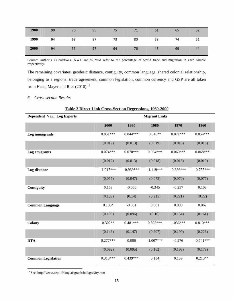
Table 2 Direct Link Cross-Section Regressions, 1960-2000

Dependent Var.: Log Exports Migrant Links

2000 1990 1980 1970 1960

Log immigrants 0.051*** 0.044*** 0.046** 0.071*** 0.054***

(0.012) (0.013) (0.019) (0.018) (0.018)

Log emigrants 0.074*** 0.078*** 0.054*** 0.060*** 0.068***

(0.012) (0.013) (0.018) (0.018) (0.019)

Log distance -1.017*** -0.939*** -1.119*** -0.886*** -0.755***

(0.055) (0.047) (0.075) (0.070) (0.077)

Contiguity 0.163 -0.066 -0.345 -0.257 0.103

(0.139) (0.14) (0.215) (0.221) (0.22)

Common Language 0.188* -0.051 0.001 0.090 0.062

(0.100) (0.096) (0.16) (0.154) (0.161)

Colony 0.302** 0.481*** 0.895*** 1.036*** 0.810***

(0.146) (0.147) (0.207) (0.199) (0.226)

RTA 0.277*** 0.086 -1.007*** -0.276 -0.741***

(0.092) (0.095) (0.162) (0.198) (0.179)

Common Legislation 0.313*** 0.439*** 0.134 0.159 0.213**

19 See: http://www.cepii.fr/anglaisgraph/bdd/gravity.htm

16

(0.061) (0.063) (0.103) (0.098) (0.108)

Common Currency -0.594*** 0.316 1.053* 1.350* 1.070***

(0.109) (0.445) (0.588) (0.72) (0.337)

Importer (i)/Exporter (j) dummies YES YES YES YES YES

Observations 3,795 3,456 3,382 3,215 2,870

R2 0.809 0.788 0.664 0.683 0.699

The dependent variable is the log of bilateral exports. All regressions include importer and exporter fixed effects. Superscripts

***, **, * denote statistical significance at 1, 5 and 10% respectively. Cluster robust standard errors are provided in parentheses.

The results of cross-section regressions, based on equation 8, are presented for the years 1960-2000 for

sample 1 (see table 2). Across all years, the regressions explain at least approximately 70% of the total

variation in bilateral exports, which is typical. The coefficient on the distance variable is around 1, which

is what theory predicts. Sharing a common border or a common language have little effect upon trade, a

result explained by the positive correlations of these variables with both migration variables, the inclusion

of other covariates which account for the variation in these variables and the implementation of importer

and exporter fixed effects. There is a very strong impact of sharing a colonial heritage, although this

effect decreases over time, as historical network effects deteriorate and institutions diverge from one

another.20

Sharing common legislative origins are also found to significantly bolster trade in three of the

five periods. The coefficients on the common currency and the RTA variables are very unstable however,

being both significantly positive and negative across the years. This is due to endogeneity bias as argued

by Glick and Rose (2002) and Baier and Bergstrand (2007) respectively.

Turning to the key variables of interest, the immigrant and emigrant variables are significant in every

decade and the coefficients are remarkably stable over time. In 2000, a 10% increase in immigrants and

emigrants is associated with bilateral trade increasing by 0.5% or 0.7% respectively. In other words, an

increase in the global stock of 8,890,000 immigrants/emigrants is associated with an increase in world

trade of $29bn and $42bn respectively, or $3,280 or $4,760 per immigrant/emigrant. In terms of the

hypotheses which have featured so strongly in the literature, the coefficient on immigrants might be

interpreted as a measure of one side of the transaction cost channel - since bilateral migration is regressed

upon unidirectional trade. Nevertheless since the coefficient on the immigrant stock variable is not

statistically larger than the coefficient on the stock of emigrants in any decade no firm conclusions can be

drawn with regards separating the two mechanisms.

20 The erosion of colonial links is well documented in Head, Mayer and Ries (2010)

17

7. Endogeneity

The importer and exporter fixed effects used in the regressions in table 1 will control for endogeneity bias

in relation to the commonly omitted multilateral resistance terms, as well as any influence of migration

among other countries on the trade between i and j. In a panel however, additional unobserved pair-wise

or country-pair-time-varying influences may exist which are correlated with the error term εij, and which

subsequently give rise to selection or an omitted variable bias. Of the three types of endogeneity that

might exist between trade and migration this is the principle cause for concern.

All efforts have been made to reduce measurement error since the two continuous variables, trade and

migration, are from official sources and the dummy variables are also taken from an authoritative dataset.

With regards simultaneity bias, sufficient evidence exists from previous studies that causality runs from

migration to trade. Hatzigeorgiou (2010) argues that trade is not a key determinate of migration and

further highlights Gould‟s test of causality which suggests that immigration precedes trade. Furthermore,

Felbermayr and Jung (2009) find that causality runs from migration to trade following a regression based

F-test of strict exogeneity. Peri and Requena (2010) using 2SLS, implement historical immigrant enclaves

as instruments for contemporaneous migration and „provide robust and consistent evidence that a causal

effect from immigrants to export flows for Spanish provinces…‟ (pg 11). Lastly, Gould argues that

immigration flows are subject to binding quotas such that migration stocks are more likely to be

exogenous than their comparable bilateral trade flows.

Omitted variable or selection bias remains worrisome however. Papers investigating the determinants of

migration by-and-large implement specifications with similar variables to those in the trade gravity model

literature. For example, economically larger countries, those in closer proximity or country-pairs sharing a

colonial heritage all tend to trade and exchange more migrants21

with one another (Ortega and Peri 2009).

In other words, the observed characteristics which drive both trade and migration are similar. Indeed, the

R2 in the handful of papers which investigate the determinants of international migration at the macro

level, are typically quite low, for example around 25% in Mayda (2007) which suggests that there exists

significant unobserved heterogeneity. In contrast, gravity models of international trade typically have an

R2 of between 60-80% (Baier and Bergstrand 2007). The question therefore is whether the unobserved

components in determining trade flows are correlated with the determinants of international migration. As

intimated by the Turkish-German example at the start of this paper, the answer is likely to be in the

affirmative.

21A variable capturing colonial links proves to be a key predictor of migrant stocks but not of migrant flows when variables for

migrant networks are included in estimation.

18

A complex combination of historical, political and cultural characteristics underpins international bilateral

relations. These characteristics are too complex to lump together under a single heading, or capture using

variables common to the gravity model literature. No doubt they have the potential to select country-pairs

into trading with, or permitting migration between, one another however, as in Turkish-German case.

These characteristics likely also constitute the fundamentals underpinning international bilateral ties. The

direction of bias given the omission of these characteristics (on trade and migration) is indeterminate

however. This is perhaps best exemplified by the fact that bilateral ties need not be congenial for trade

and migration to exist. Countries with „good‟ bilateral ties might experience trade and migration (Brazil

and Japan), trade and no significant migration (United Kingdom and Mexico), migration and no

significant trade (Sweden and Serbia and Montenegro) or negligible trade and migration (France and

Bhutan). However, so too can „bad‟ bilateral ties give rise to similar outcomes. Poor relations still

underpin trade and migration between Iran and the United States.22

Strained ties between Germany and

Myanmar, while not resulting in significant migration, still give rise to significant trade. The Cuban

diaspora in the US is the 11th largest South-North corridor in the world (Özden et al 2011)

23 and

negligible trade and migration occur between Israel and Malaysia.

These deep-rooted (and yet unobservable) historical, cultural or political country-pair characteristics, may

thus be positively or negatively correlated with both trade and migration, which in turn might lead to

either over- or under-estimates of the effect of migration on trade. However, (as similarly argued by Baier

and Bergstrand (2007)) if these characteristics are fundamental in nature and have endured over time, then

they will likely affect the levels of trade and migration (relative to their potential), as opposed to recent

changes in trade and migration. If true, then these deterministic characteristics will be predominantly

cross-sectional in nature and can be largely accounted for with country-pair fixed effects; the

implementation of which will also control for the endogeneity of the RTA and Currency Union dummies.

8. Panel Results

In a panel framework, equation 8 can be rewritten as:24

9.

22 In 2000, the Iranian diaspora in the United States was the 22nd largest, while the United States was the 21st most important

export market for Iran. 23 In 2000, the 577 Americans recorded as residing in Cuba represented the fifth largest diaspora in the Caribbean Island. 24 Here the left-hand side is not divided through by the product of the national income variables a la Baier and Bergstrand (2007),

since no restriction of unitary income elasticises is imposed.

19

In addition to the fixed effects to control for multilateral resistances which now have a t subscript, the

term, τij, is a vector of bilateral i and j fixed effects. Four regressions are presented (see table 3). The first

includes importer, exporter and year dummies and can be thought of as the simple model. The next

implements importer/exporter-time-varying dummies, which as well as appropriately accounting for

deflating current prices through the time dummies also control for multilateral resistances (Baldwin and

Taglioni 2006). The last two specifications include both importer/exporter-time-varying and pair-wise

dummies but differ in how the pair-wise dummies are constructed. The results in the third column,

implement fixed effects (termed pair) on country-pairs, regardless of the direction of trade. The dummy

for the Franco-Belgian bilateral tie for example therefore equals one whether France exports to Belgium

or Belgium exports to France. In the last column, separate pair-wise dummies are used for each direction

of bilateral trade flows (termed pairid). Pair fixed effects are justified if trade costs really are symmetric.

Pairid fixed effects are analogous to the standard „within‟ panel estimator. All robust standard errors are

clustered by country-pair.

The simple model yields results familiar from the literature and comparable to the cross-section results in

table 1. The log of immigrants and emigrants are both highly significant and with the coefficient on

emigrants larger than that of immigrants, which is expected due to the addition of preferences operating in

the same direction as trade. The results in the second column, which additionally control for multilateral

resistances, are similar to those in the first column, although the standard errors are marginally broader. In

other words, - with the exception of the coefficient on the currency union variables - there seems to be

little bias resulting from failing to account properly for multilateral resistance. That is not to detract from

the results of Felbermayr, Jung and Toubal (2009) however, whom provide convincing evidence that a

failure to include importer and exporter fixed effects in cross-section analyses leads to significant biases.

Table 3 Direct Link Pooled Regressions, 1960-2000

Dependent Var.: Log Exports Migrant Links

1 2 3 4

Log immigrants 0.061*** 0.055*** -0.023* -0.023*

(0.009) (0.010) (0.012) (0.013)

Log emigrants 0.073*** 0.070*** -0.011 -0.009

(0.009) (0.010) (0.012) (0.015)

Log distance -0.929*** -0.938*** . .

(0.043) (0.045) . .

20

Contiguity -0.063 -0.107 . .

(0.130) (0.137) . .

Common Language 0.057 0.0467 . .

(0.094) (0.097) . .

Colony 0.690*** 0.748*** . .

(0.150) (0.153) . .

RTA -0.166*** -0.015 0.486*** 0.490***

(0.065) (0.073) (0.069) (0.074

Common Legislation 0.249*** 0.262*** . .

(0.057) (0.058) . .

Common Currency 0.123 0.319* 0.637*** 0.640***

(0.180) (0.188) (0.150) (0.157)

Importer /Exporter dummies (i/j) YES

Year dummies (t) YES

Importer/Exporter-time-varying dummies (it/jt) YES YES YES

Symmetric pair dummies (ij) YES

Asymmetric pair dummies (ij) YES

Observations 16,718 16,718 16,718 16,718

R2 0.734 0.780 0.866 0.901

The dependent variable is the log of bilateral exports. All regressions include importer and exporter fixed effects. Superscripts

***, **, * denote statistical significance at 1, 5 and 10% respectively. Robust standard errors are provided in parentheses.

When the pair or symmetric fixed effects are additionally included, the results change dramatically. The

RTA and common currency dummies are now highly positive and similar to those obtained by Glick and

Rose (2002) who found a coefficient of 0.74 and Baier and Bergstrand (2007) who estimated the impact

of RTAs on trade to be 0.68. Since Rose (2002) uses symmetric fixed effects, these results would

vindicate his approach.

Most importantly for the purposes of this paper however, are the results on both migration variables. No

effect of emigrants is found whatsoever and the coefficient on the immigrant variable is actually negative,

21

suggesting that a 10% rise in immigrants is associated with a 0.2% fall in trade. Theory suggests that the

unobserved bilateral factors, which are captured here using country-pair fixed effects, may be both

positively and negatively correlated with migrant networks. The empirical results clearly demonstrate

however, that on average these unobserved bilateral factors are strongly positively correlated with the

migration variables, such that their imposition removes the positive impact of migration on trade.

Previous estimates which fail to control for these factors should be treated with caution therefore. One

possible explanation is offered by Diaz-Alejandro (1970), who argues that migrants might start producing

in the destination country those goods that they previously demanded from abroad. More simply, this

might be a pure demand effect such that immigrants continue consuming destination country products

once they have left the origin country. The results in the final column, using asymmetric pair-wise fixed

effects, those akin to the standard „within‟ estimator, yield similar results. According to the theory, trade

costs are treated symmetrically. Clearly, in reality this might not be the case however. The foregoing

results would suggest that empirically, at the aggregate level at least, it is not important which set of fixed

effects are used since the results are not significantly different from one another.

Since no study to the knowledge of the author, has crucially controlled for the age on arrival of migrants,

little evidence currently exists as to the persistence of the effect of migrants upon trade over time. Since

the estimated panel contains observations at ten-year intervals, one interpretation of the results is that they

more adequately pick up the long-run relationship between trade and migration, a steady-state estimate

once capital has had time to adjust. It might also be the case that migrants only facilitate trade between

those countries which are absent from the sample. Given the proportions of trade and migration covered

in the sample however - which also include many countries for which positive effects have been found in

the existing literature – this also seems unlikely.

Of course the implementation of fixed effects is no panacea, although this is the strategy adopted to

control for the endogeneity bias of currency unions and regional trade agreements elsewhere in the

literature. First they treat both positive and negative correlations of the unobserved pair-wise factors with

the migrant network variables as symmetric. A further cause for concern is attenuation bias. Should one

of the right-hand side variables be poorly measured, this would lead to a classic error-in-variables

problem whereby differencing the panel data biases the resulting estimates towards zero. This is

especially the case should the variable in question be largely time-invariant. However, in terms of both

the aggregate immigrant and emigrant stocks and the bilateral pair-wise migration corridors, there have

been dramatic changes over time, such that this is not a cause for concern. Moreover, the classic error-in-

variables generally leads to inconsistent estimates of all the βs and since the estimates of the other

22

explanatory variables are strictly in line with previous estimates, this provides indirect evidence that the

estimates can be trusted.

8.1 Robustness

Lastly, it might be the case that some of the missing values, which we have every reason to believe are

true missing values, are in fact zero. If so, then a failure to account for the heteroskedastic residuals,

which arise from numerous zero values in the regressor, might lead to inconsistent results. Table 4

provides a summary of how many missing values exist in every decade.

Table 4 % Missing values in sample 1, 1960-2000

Decade % Missing

1960 27

1970 18

1980 13

1990 12

2000 9

Source: Author‟s Calculations.

Table 5 Pooled Regressions to test for robustness

Dependent Var.: Log Exports Migrant Links

Sample 2 Sample 1

No 1960

Sample 3 Sample 4

Log immigrants -0.005 -0.012 -0.025** -0.024*

(0.013) (0.016) (0.013) (0.014)

Log emigrants -0.018 -0.009 0.016 0.020

(0.012) (0.017) (0.016) (0.020)

RTA 0.439*** 0.498*** 0.380*** 0.429***

(0.068) (0.067) (0.069) (0.081)

Common Currency 0.522*** 0.506*** 0.458*** 0.380***

(0.146) (0.112) (0.118) (0.129)

23

Importer/Exporter-time-varying dummies (it/jt) YES YES YES YES

Asymmetric pair dummies (ij) YES YES YES YES

Observations 30,625 13,848 10,387 7,876

R2 0.654

a 0.681

a 0.814

a 0.833

a

The dependent variable is the log of bilateral exports. All regressions include importer and exporter fixed effects. Superscripts

***, **, * denote statistical significance at 1, 5 and 10% respectively. Robust standard errors are provided in parentheses. a

denotes that the estimated R2 is not comparable to the R2 in other tables since it is calculated using the standard within estimator

as opposed to the least squares dummy variable estimator. This is to ensure consistency within the table since it is not possible to

use the LSDV for sample 1 since it is beyond the limits of Stata.

Clearly the greatest number of missing values is in 1960, which is expected given the timing of the onset

of globalization. In order to test for the inclusion of the missing values, table 5 provides further estimates.

Column 2, estimates equation [9] on sample 2, the full sample of 68*178 countries. Column 3 again

estimates sample 1, but this time excluding the year 1960, the year which comprises the greatest

proportion of missing values. Column 4 provides estimates for sample 3, a sub-sample which comprises

only those origins with fewer than 30 missing values; while column 5 presents the estimates for sample 4,

a sub-sample which comprises the fewest missing values, with the regression estimated on those exporters

which report fewer than 20 missing values. The results are remarkably stable across all five samples.

None of the estimates on either the currency union or the RTA variables are statistically different from

one another and no statistically significant effect of emigrants on exports is found in any of the samples.

Similarly, the estimated impact of immigrants on trade is either negative or insignificantly different from

zero across all five samples. The results in table 5 therefore lend credibility to the main estimates, since it

is clear the results are not an artifact of either sample selection or the inclusion of the missing values.

9. Regional Results

Given the weight of evidence in the literature to date, the results pooling observations across the entire

sample are very surprising. Given Winters‟ insight that the least similar countries have the greatest

potential for trade however, the sample is next divided into the relatively affluent North25

and

comparatively poorer South. Two regressions are estimated for each regional combination. The first

column presents results akin to column 2 of table 3, when country-time varying dummies are included but

country-pair fixed effects are not. The results in the second column present the most restrictive

specification, which then additionally include asymmetric (pairid) fixed effects (see table 6).

25

The countries of the „North‟ refer to those countries that have been consistently wealthy throughout the period i.e. the countries

of the OECD minus the Czech Republic, Hungary, Korea, Mexico, Poland the Slovak Republic and Turkey.

24

The first set of regional results, those from columns (1), omit controls for unobserved pair-factors and

again produce the results typically found in the literature. The coefficient on distance is again around

minus 1, the negative impact of which disproportionately affects Southern exporters. While again the

contiguity variable is insignificant across all specifications, the role of common language, a proxy for

cultural proximity, is significantly positive for trade between the North and the South. Sharing a colonial

heritage is again found to strongly influence trade, except in the case of Southern exports to the North.

Similarly, sharing a common legislative system positively impacts trade except for Northern exports to

the South. While few inferences can be drawn with regards the RTA or common currency variables, due

to the well-documented endogeneity bias which exists in their presence, positive coefficients result.

Importantly, in the absence of pair-wise fixed effects, all the coefficients on the immigrant and emigrant

stock variables are highly significant and positive with the exception of the effect of Northern immigrants

on Southern exports.

Again however, the results for all four regional combinations alter dramatically once controls are added

for unobserved heterogeneity. Regional trade agreements are then only found to positively influence

exports between countries of the North. Similarly, sharing a common currency is only found to boost

Northern exports to Southern countries. The most startling results however again concern the migration

variables. Immigrants and emigrants are only found to influence aggregate bilateral trade flows for

exports from the North to the South and even in this case the estimates are smaller than many papers in

the literature would suggest. Since the degree of differentiation of exported goods is likely far higher from

countries of the North, and since informational asymmetries are likely highest between countries of the

North and the South; migrants might be expected to influence trade the most between the North and the

South a priori. The failure to uncover an impact of migration upon trade is most surprising in the context

of North-North trade. Here, over 98% of the variation in bilateral trade is explained, the trade and the

migration data are of the highest quality and exports are likely the most differentiated. One plausible

explanation for this result would be that information is more readily available about the countries of the

North such that migrants cannot exert much influence in terms of bridging informational asymmetries.

Table 6 Direct Links Regional Regressions, 1960-2000

Dependent Var.: Log

Exports

Migrant Links

N-N (1) N-N (2) S-N (1) S-N (2) N-S (1) N-S (2) S-S (1) S-S (2)

Log immigrants 0.040*** 0.010 -0.005 -0.005 0.083*** 0.033* 0.048*** -0.029

(0.015) (0.016) (0.022) (0.034) (0.017) (0.017) (0.017) (0.030)

25

Log emigrants 0.040** 0.011 0.106*** 0.016 0.054*** 0.055** 0.058*** -0.016

(0.018) (0.018) (0.019) (0.022) (0.018) (0.026) (0.016) (0.034)

Log distance -0.824*** . -1.041*** . -0.863*** . -1.318*** .

(0.062) . (0.092) . (0.080) . (0.081) .

Contiguity 0.084 . 0.487 . 0.162 . -0.112 .

(0.085) . (0.476) . (0.477) . (0.206) .

Common Language 0.044 . 0.329** . 0.334** . 0.080 .

(0.087) . (0.156) . (0.150) . (0.155) .

Colony 0.406*** . 0.163 . 0.525*** . 0.932* .

(0.134) . (0.211) . (0.178) . (0.508) .

RTA 0.403*** 0.267*** 0.085 0.115 0.245* 0.253 -0.095 0.096

(0.074) (0.059) (0.198) (0.216) (0.148) (0.178) (0.165) (0.267)

Common Legislation 0.311*** . 0.295*** . -0.044 . 0.216** .

(0.063) . (0.098) . (0.081) . (0.095) .

Common Currency 0.305*** 0.199 1.504** 1.093* 1.226** 0.36 0.000 0.831

(0.125) (0.123) (0.613) (0.644) (0.506) (0.394) (0.423) (0.741)

Importer /Exporter time-

varying dummies (it/jt) YES YES YES YES YES YES YES YES

Asymmetric pair dummies

(ij) . YES . YES . YES . YES

Observations 2,088 2,088 4,187 4,187 4,269 4,269 6,174 6,174

R2 0.959 0.985 0.788 0.930 0.847 0.894 0.671 0.857

The dependent variable is the log of bilateral exports. All regressions include importer and exporter fixed effects. Superscripts

***, **, * denote statistical significance at 1, 5 and 10% respectively. Robust standard errors are provided in parentheses.

The only paper, with estimates directly comparable to those presented here however, are those provided

by Felbermayr and Jung (2009), since, as argued throughout the paper, cross-sectional results should be

viewed with caution given that other bilateral factors, which might drive both trade and migration cannot

be accounted for. They estimate a panel of North-South trade and migration for 1990 and 2000 using the

26

„within‟ estimator, which yields a coefficient on the stock of immigrants from the South in the North of

0.112, (with a standard error of 0.043). Given the various differences between the approached adopted,

the results here are considered consistent with their findings.26

10. Country Results

The results so far relate to the average effect of both immigrants and emigrants upon trade, either across

countries (table 2), over time (tables 3 and 5) or across regions and time (table 6). In each case,

controlling for unobserved pair-wise factors removes most if not all of the positive affect of migration

upon trade. The results may be further decomposed by interacting the immigrant variable with the 68

destinations and the emigrant variable by the 68 origins (equation 10), to yield the average effects of these

variables for specific countries over time.

10.

Where, π1 and π2 are coefficient vectors for the interaction variables. This exercise pushes the data to the

very limit, since only four/five observations are available for each country. The goal then, is not to draw

firm inferences with regards point estimates at the country level, but rather to get a better sense of the

direction of bias which results from failing to take account of unobserved pair-wise heterogeneity. The

statistically significant coefficients for the immigrant interactions from [10], from both including and

omitting τij are presented in Table 7. Due to their similarity, the emigrant interactions are presented in

Appendix 2 for the sake of brevity

Table 7 again serves to highlight the disparity in the results when unobserved factors are omitted. In the

absence of pair-wise fixed effects, 35 countries have statistically significant immigrant-interaction point

estimates, while 33 countries have statistically significant emigrant-interaction point estimates. While the

overwhelming majority of these point estimates are positive, importantly, some statistically significant

and negative coefficients also result i.e. trade diversion. Although this finding is largely absent from the

literature it seems wholly plausible since networks might well; organize the production of a good that was

previously imported from elsewhere, source these goods from third-party countries or otherwise find

more profitable destinations for goods. In order to do this, direct migrant networks might tap into their

26 Felbermayr and Jung omit the effect of Northern migrants residing in Southern countries, which might bias their estimate

upwards. Their time period is shorter, they take the average of trade flows over time to smooth the trade data, implement the

geometric average of trade flows in estimation while their migration data only captures migrants 25 and over.

27

wider international networks, which although an interesting possibility is beyond the scope of the current

study.

Table 7: Results for Country-level Immigrant Interactions

Country Mig. Stock Coeff. No τij Sig. Coeff. Inc. τij Sig. Country Mig. Stock Coeff. No τij Sig. Coeff. Inc. τij Sig.

Australia-Norfolk Is. 240,778 0.20 *** -0.02

Hong Kong SAR, China 287,117 0.11 *** -0.01

Philippines 1,237,433 0.19 *** 0.05

Oman 75,655 0.11 * -0.08

Venezuela 162,537 0.19 *** -0.01

Slovenia 13,231 0.11 **

Angola 172,856 0.18 ** -0.19 *

South Africa-

Botswana-Lesotho-

Namibia-Swaziland 203,721 0.11 ** -0.03

Chile 342,971 0.18 *** -0.12

United Arab Emirates 17,467 0.09 * -0.09

Malaysia 494,239 0.18 *** 0.04

Pakistan 5,621,668 0.09 -0.14 *

Peru 231,434 0.18 *** -0.07

Tunisia 426,364 0.09 *** -0.07

Dominican Rep. 330,979 0.17 *** 0.03

Norway 192,642 0.09 ** 0.07

Israel 125,829 0.15 ** 0.04

Thailand 168,634 0.09 *** -0.07

Ecuador 221,108 0.15 *** -0.10

Finland 316,196 0.06 * 0.16 *

Mexico 3,607,198 0.15 *** -0.10

Greece 938,753 0.06 ** 0.00

New Zealand 242,460 0.15 *** -0.02

Turkey 1,733,521 0.05 * -0.11 * Indonesia-East

Timor-Maldives 742,776 0.14 *** -0.03

Germany 2,840,813 -0.06 ** 0.04

Russia 796,637 0.14 ***

Belgium-Luxembourg 311,149 -0.06 ** -0.10

Colombia 723,293 0.14 *** -0.08

Netherlands 670,888 -0.08 ** -0.03

Canada 1,115,927 0.14 *** -0.21 *** France-Monaco-

Andorra 1,045,326 -0.08 *** -0.09

Qatar 1,586 0.12 * -0.06

Saudi-Arabia 56,140 -0.09 * -0.17 **

Argentina 253,322 0.12 ** -0.13

Czechoslovakia 1,014,715 -0.10 * -0.18

Superscripts ***, **, * denote statistical significance at 1, 5 and 10% respectively.

When unobserved pair-wise factors are accounted for, again the majority of these positive effects

disappear. It was argued in the endogeneity section, that in theory, the direction of the bias from failing to

account for the unobserved heterogeneity could work in either direction. This plays out, for example the

point estimate for Finland increases from 0.06 to 0.16 following the inclusion of τij. Conversely, the

coefficient for Canada falls from 0.14 to -0.21. However, the global and regional estimates suggest that

overall; the unobserved bilateral factors are positively correlated with migrant networks on average, such

that their inclusion dramatically removes most of the effect of migration upon trade. This story is again

borne out by these results, since the vast majority of positive estimates are found to be insignificant or

indeed significant and negative when fixed effects are included.

11. Third Party Effects

28

So far, attention has been focused upon direct links. It is equally plausible however; that migrant

networks exist between trading pairs which pertain to a country (of birth) k, which is neither the importing

(k≠i) nor exporting nation (k≠j) i.e. that a third-party effect exists which is driving the observed

coefficients.27

Continuing from the discussion in Section 3, these third party effects can be modeled as

ln(MIGki*MIGkj) where i≠j and k≠i and k≠j. This is another important contribution of this paper, since

despite only 68 countries being chosen for analysis; the comprehensive migration dataset permits third-

party effects pertaining to potentially all (178) countries of the world to be included in estimation (see

Equation 11).

11.

Where additionally, ς1 is a vector containing the coefficients for the interactions of the third-party effects.

Table 8 again presents the statistically significant point estimates for the third-party effects estimated in

[11] while both omitting and including τij. The estimates of the indirect effects of migrants are more stable

in comparison with the existing literature, whether or not pair-wise fixed effects are included in the

regression. Prior to the inclusion of τij, there are 30 positive and 29 negative point estimates; suggesting in

comparison with direct effects third-party networks are more likely to divert trade.

It is not as immediately obvious why pair-wise fixed effects should be implemented when testing for

third-party effects. Felbermayr, Jung and Toubal (2009) argue that third-party effects should be

exogenous to bilateral trade flows between countries i and j, since the migrants pertain to countries k.28

However, if migrants from a country k are believed to foster trade between countries i and j then there

might be unobserved bilateral factors between i and j, which encourage migrants from k to select into

migrating into those countries in the first place. In fact, controlling for pair-wise unobserved factors again

drastically alters the results, with only 15 point estimates surviving. In the case of third-party effects

however, the direction of the bias from excluding controls for the unobserved pair-wise factors is far from

clear, since many estimates are both biased up and down. This result contrasts nicely with the estimates of

the direct results. In that case, the direction of the bias was on average positive, which might be expected

since international bilateral ties are more generally „good‟ as opposed to „bad‟ and in turn these good

relationships might be expected to be positively correlated on average with migrant networks. In the case

of indirect networks however, the results suggest a far more complex relationship. Arguably, these

complexities can only be identified with richer more disaggregated data.

27 Felbermayr, Jung and Toubal (2009) are credited as having been the first to highlight the difference between direct and indirect

links. 28

Furthermore they argue that these third-party effects must operate though the transaction cost channel.

29

Table 8: Results for Country-level Indirect Interactions

Country Mig. Stock Coeff. No τij Sig. Coeff. Inc. τij Sig. Country Mig. Stock

Coeff. No

τij Sig.

Coeff. Inc.

τij Sig.

Latvia 54,554 0.12 *** 0.04

Iceland 19,205 0.00 -0.02 *

Cameroon 41,478 0.07 *** 0.04

Myanmar 214,829 0.00 0.03 **

United Kingdom 3,649,716 0.06 *** -0.12 **

Antigua-British

Virgin Is.-

Dominica-Grenada-

Montserrat-St

Kitts-Anguilla-St

Lucia-St Vincent 91,348 -0.01 -0.02 *

Nepal 612,465 0.06 *** 0.02

Peru 231,434 -0.02 0.04 *

Japan 564,264 0.05 *** 0.02

Egypt 1,021,589 -0.02 0.04 *

Iran 446,783 0.05 *** 0.04

Jamaica-Turks and

Caicos-Cayman Is. 459,221 -0.02 ** -0.01

India 6,361,587 0.05 * -0.04

Bahamas 16,859 -0.02 * 0.01

Romania 976,563 0.05 * 0.06

Bhutan-Brunei 36,197 -0.02 ** 0.00

Czechoslovakia 1,014,715 0.05 * 0.03

Philippines 1,237,433 -0.03 * 0.00

Guatemala 192,359 0.04 ** 0.00

Congo 17,777 -0.03 * -0.03 France-Monaco-

Andorra 1,045,326 0.04 ** 0.04

Greenland 5,418 -0.03 ** 0.00

Guyana 134,275 0.04 *** 0.00

Gibraltar 10,984 -0.03 ** -0.01

Germany 2,840,813 0.04 ** -0.02

Ghana 158,859 -0.03 * 0.00 Trinidad and Tobago 138,159 0.04 *** 0.00

Portugal 1,373,239 -0.03 ** 0.01

Denmark-Faeroe

Islands 203,767 0.04 *** 0.03

Australia-Norfolk Is. 240,778 -0.03 * 0.00 Guinea-Bissau-

Cape Verde-Sao

Tome y Principe 86,609 0.03 *** 0.00

Laos 156,926 -0.03 ** -0.01

Samoa 38,689 0.03 *** 0.01

Venezuela 162,537 -0.03 *** 0.00 Belgium-

Luxembourg 311,149 0.03 * 0.00

Mexico 3,607,198 -0.04 *** 0.00 Bosnia and Herzegovina 159,234 0.03

0.12 *** Colombia 723,293 -0.04 ** -0.02

North Korea 403,285 0.03 *** 0.01

Central African Republic 3,725 -0.04 ** 0.00

Brazil 300,387 0.03 ** 0.00

Democratic Republic of Congo 41,717 -0.04 *** -0.02

Seychelles 4,276 0.03 * 0.04 ** Malta 90,044 -0.04 *** -0.02

Korea 1,211,822 0.03 ** 0.00

Suriname 103,078 -0.04 *** -0.02

Spain 1,631,399 0.03 * 0.01

Falklands 647 -0.04 * -0.02

Papua New Guinea 17,593 0.03 * -0.02

Israel 125,829 -0.04 ** -0.02

Sudan 140,239 0.02 * -0.02

Mongolia 2,118 -0.04 *** 0.01 Netherlands

Antilles-Aruba 65,811 0.02 *** 0.02

Djibouti 1,369 -0.04 *** -0.03

Bahrain 9,983 0.02 * 0.00

Gambia 8,351 -0.05 *** -0.03

Thailand 168,634 0.02 * 0.02

Vietnam 640,323 -0.05 *** -0.02

Ecuador 221,108 0.02 * 0.03 ** Slovenia 13,231 -0.05 *** -0.01

Macao 424,121 0.02 *** 0.01 * Saudi Arabia 56,140 -0.05 *** -0.05 ***

Algeria 1,354,783 0.01

-0.01

Estonia 38,333 -0.06 ** -0.05 *

Syria 274,244 0.01

-0.04 ** Slovakia 106,463 -0.06 *** -0.15 ***

Malaysia 494,239 0.00

-0.03 ** Kazakhstan 538,338 -0.08 ** 0.01

Superscripts ***, **, * denote statistical significance at 1, 5 and 10% respectively.

12. Conclusion

30

Do migrants really foster trade? The answer based on the results in this paper would be a tentative Yes.

Abstracting from the question of how migrants foster trade, the key question asked in this paper is

whether migrants foster trade whatsoever. Implementing a panel which comprises the majority of world

trade and migration in each period, the core results show that a failure to account for unobserved pair-

wise heterogeneity, which in turn is positively correlated with migrant networks, lead to a substantial

overestimate of the impact of migration on trade. The estimates imply that in the longer run, migration

has a negligible or indeed negative impact on trade. Dividing the world into the relatively affluent North

and poorer South, the results show that migrants from either region only affect Northern exports to the

South. Further, the country level results suggest that migrants may both create and divert international

trade. Taken as a whole, the results demonstrate the large biases inherent in cross-sectional studies

investigating the trade-migration nexus and highlight the need to be cautious when interpreting previous

findings. The surprise therefore is not that few positive effects are found, but rather that such

unambiguously positive and robust results have featured so prominently in the literature to date. While an

international examination of the trade-migration nexus at the product level is absent from the existing

literature, the results from this paper strongly suggest that this should be a research priority should the

complexities of the trade-migration nexus be truly understood.

Bibliography

31

Anderson, J. E., and van Wincoop, E., (2003), "Gravity with Gravitas: A Solution to the Border Puzzle",

American Economic Review, vol. 93(1), pages 170-192, March.

Anderson, J. E., and van Wincoop, E., (2004), "Trade Costs," Journal of Economic Literature, American

Economic Association, vol. 42(3), pages 691-751, September.

Baier, S. L., and Bergstrand, J. H., (2007), "Do free trade agreements actually increase members'

international trade?", Journal of International Economics, Elsevier, vol. 71(1), pages 72-95, March.

Baldwin, R. E. and Taglioni, D., (2006), “Gravity for Dummies and Dummies for Gravity Equations”,

CEPR Discussion Paper No. 5850. Available at SSRN: http://ssrn.com/abstract=945443

Bandyopadhyay, S., et al, (2008), “Ethnic Networks and U.S. Exports”, (2006), Review of International

Economics, 16, issue 1, p. 199-213.

Bardhan, A.D., and Guhathakurta, S., (2004), "Global Linkages of Subnational Regions: Coastal Exports

and International Networks," Contemporary Economic Policy, Western Economic Association

International, vol. 22(2), pages 225-236, 04.

Blanes-Cristóbal, J.V., (2003), "The link between immigration and trade in Spain", Seville, Universidad

Pablo de Olavide, Paper presented at XXVIII Simposio de Análisis Económico, 11-13 December, Seville.

Bryant, J., et al, (2004), "Trade and Migration to New Zealand", Treasury Working Paper Series 04/18,

New Zealand Treasury.

Cheng, I-H., and Wall, H. J., (2004), “Controlling for heterogeneity in gravity models of trade and

integration”, Working Papers, Federal Reserve Bank of St. Louis, No 1999-010.

Co, C.Y., P. Euzent and Martin T., (2004), "The export effect of immigration into the USA", Applied

Economics, vol. 36(6), pages 573-583, April.

Combes, P., et al (2005), “The trade-creating effects of business and social networks: evidence from

France”, Journal of International Economics, vol. 66, issue 1, pages 1-29.

Diaz-Alejandro, C.F., (1970), “Essays on the Economic History of the Argentine Republic”, Yale

University Press: New Haven, CT.

Dunlevy, J., and Hutchinson W., (1999), “The Impact of Immigration on American Import Trade in the

Late Nineteenth and Twentieth Centuries”, Journal of Economic History 59 (4): 1043–1062.

Dunlevy, J., and Hutchinson W., (2001), „The pro-trade effects of immigration on American exports

during the period 1870 to 1910‟,Vandablit University Working Paper 01-W25.

Dunlevy, J., (2006), “The Influence of Corruption and Language on the Protrade Effect of Immigrants:

Evidence from the American States”, Review of Economics and Statistics 88(1).

Feenstra, R., (2004), “Advanced International Trade: Theory and Evidence”, Princeton University Press,

Princeton, NJ.

Feenstra, R., et al, (2005) “World Trade Flows: 1962-2000”, NBER Working Paper Series, Vol. w11040.

Felbermayr, G.J., and Toubal, F., (2008), “Revisiting the Trade-Migration Nexus: Evidence from New

OECD Data”, Available at SSRN: http://ssrn.com/abstract=1144063.

Felbermayr, G.J., et al (2009), "Ethnic Networks, Information, and International Trade: Revisiting the

Evidence," Diskussionspapiere aus dem Institut für Volkswirtschaftslehre der Universität Hohenheim

306/2009, Department of Economics, University of Hohenheim, Germany.

32

Girma, S., and Yu, Z., (2002), “The link between immigration and trade: evidence from the UK‟,

Weltwirtschaftliches Archive.

Glick, R., and Rose, A, (2001), Does a Currency Union Affect Trade? The Time Series Evidence, No

8396, NBER Working Papers, National Bureau of Economic Research, Inc.

Gould, D., (1994), “Immigration Links to the Home Country: Empirical Implications for US Bilateral

Trade Flow”, Review of Economic and Statistics 76 (2): 302–316.

Hanson, G., (2010), “International Migration and Development,” in Ravi Kanbur and A. Michael Spence,

eds., Equity ina Global World, Washington, DC: The World Bank.

Hatzigeorgiou, A., (2010), “Migration as Trade Facilitation: Accessing the Links between International

trade and migration”, submitted to B.E. Journal of Economic Analysis and Policy.

Hatzigeorgiou, A. (2009), “Does Immigration Stimulate Foreign Trade? Evidence from Sweden”, Journal

of Economic Integration.

Head, K., and Ries J., (1998), “Immigration and Trade Creation: Econometric Evidence from Canada”,

Canadian Journal of Economics 31 (1): 47–62.

Head, K., et al, (2010) “The erosion of colonial trade linkages after independence”, Journal of

International Economics, Volume 81, Issue 1, May 2010, Pages 1-14.

Herander, M. G., and Saavedra, L. A., (2005), “Exports and the Structure of Immigrant-Based Networks:

The Role of Geographic Proximity”, The Review of Economics and Statistics, 87, issue 2, p. 323-335.

Lucas, R., (2008), “International Migration and Economic Development”, Edward Elgar Publishing.

Mayda, A. M., (2007), “International migration: A panel data analysis of the determinants of bilateral

flows”, No 0707, CReAM Discussion Paper Series, University College London.

McMurray, J., (2001), “Distant Ties: Germany, the Ottoman Empire, and the Construction of the

Baghdad Railway”, Praeger.

Ortega, F. and Peri, G., (2009), “The Causes and Effects of International Labor Mobility: Evidence from

OECD Countries 1980-2005”, MPRA Paper, University Library of Munich, Germany.

Özden , C., et al, (2011) “Where on Earth is Everybody? The Evolution of International Bilateral Migrant

Stocks 1960-2000”, World Bank Economic Review.

Peri, G., and Requena, F., (2010), “The Trade Creation Effect of Immigrants: Evidence from the

Remarkable Case of Spain”, Canadian Journal of Economics, 43, issue 4, p. 1433-1459.

Rauch, J.E., (2001), "Business and Social Networks in International Trade", Journal of Economic

Literature, vol. 39(4), pages 1177-1203, December.

Rauch, J.E., and Trindade, V., (2002), "Ethnic Chinese Networks In International Trade", Review of

Economics and Statistics, vol. 84(1), pages 116-130, February.

Ravenstein, E. G., (1885), “The Laws of Migration, Journal of the Statistical Society, Vol. 48, No. 2, pp. 167-235.

Rose, A., (2000), “One money, one market: the effect of common currencies on trade”, Economic Policy,

15, issue 30, p. 7-46

Rose, A., K., and van Wincoop, E., (2001), "National Money as a Barrier to International Trade: The Real

Case for Currency Union", American Economic Review, vol. 91(2), pages 386-390, May.

33

Santos Silva, J. M. C., and Tenreyro, S., (2006), "The Log of Gravity", Review of Economics and

Statistics, MIT Press, vol. 88(4), pages 641-658, 09.

Wagner, D., et al, (2002), “Immigration and the Trade of Provinces”, Scottish Journal of Political

Economy, Vol. 49, pp. 507-525, 2002.

White, R., (2007b), “An Examination of the Danish Immigrant-Trade Link,” International Migration 45,

5: 62-86 (December).

Winters, L.A., (2003), „The Economic Implications of Liberalizing Mode 4 Trade‟, in A. Mattoo and A.

Caarsaniga (Eds) Moving People to Deliver Services, World Bank, Washington D.C.

34

Appendix 1: List of Countries in each sample

Sample 1

Algeria Czech Republic Indonesia-East

Timor-Maldives Morocco Romania Tunisia

Angola Czechoslovakia Iran Netherlands Russia Turkey

Argentina Denmark-Faeroe

Islands Ireland

New Zealand-Cook

Islands-Niue-

Tokelau

Saudi Arabia United Arab

Emirates

Australia-Norfolk Is. Dominican Republic Israel Nigeria Singapore United Kingdom

Austria Ecuador Italy Norway Slovakia United States-Puerto

Rico-US Virgin Is.

Belgium-

Luxembourg Finland Japan Oman Slovenia Venezuela

Brazil France-Monaco-

Andorra Kazakhstan Pakistan

South Africa-

Botswana-Lesotho-

Namibia-Swaziland

Vietnam

Bulgaria Germany Korea Peru Soviet Union Fm. Yugoslavia

Canada Greece Kuwait Philippines Spain

Chile Hong Kong SAR,

China Libya Poland Sweden

China Hungary Malaysia Portugal Switzerland-

Liechtenstein

Colombia India Mexico Qatar Thailand

Sample 2

Afghanistan Central African

Republic Georgia Kyrgyz Republic North Korea St. Helena

Albania Chad Germany Laos Norway St. Pierre and

Miquelon

Algeria Chile Ghana Latvia Oman Sudan

Angola China Gibraltar Lebanon Pakistan Suriname

Antigua-British

Virgin Is.-Dominica-

Grenada-Montserrat-

St Kitts-Anguilla-St

Lucia-St Vincent

Colombia Greece Liberia Panama Sweden

Argentina Congo Greenland Libya Papua New Guinea Switzerland-

Liechtenstein

Armenia Costa Rica Guatemala Lithuania Paraguay Syria

35

Australia-Norfolk

Islands Cote d'Ivoire Guinea Macao Peru Tajikistan

Austria Croatia

Guinea-Bissau-Cape

Verde-Sao Tome y

Principe

Macedonia Philippines Tanzania

Azerbaijan Cuba Guyana Madagascar Poland Thailand

Bahamas Cyprus Haiti Malawi Portugal Togo

Bahrain Czech Republic Honduras Malaysia Qatar Trinidad and Tobago

Bangladesh Czechoslovakia Hong Kong SAR,

China Mali Reunion-Comoros Tunisia

Barbados Democratic Republic

of Congo Hungary Malta Romania Turkey

Belarus Denmark-Faeroe

Islands Iceland

Guadeloupe-

Martinique Russia Turkmenistan

Belgium-

Luxembourg Djibouti India Mauritania Rwanda Uganda

Belize Dominican Republic Indonesia-East

Timor-Maldives Mauritius Samoa Ukraine

Benin Ecuador Iran Mexico Saudi Arabia United Arab

Emirates

Bermuda Egypt Iraq Moldova Senegal United Kingdom

Bhutan-Brunei El Salvador Ireland Mongolia Serbia United States-Puerto

Rico-US Virgin Is.

Bolivia Equatorial Guinea Israel Morocco Seychelles Uruguay

Bosnia and

Herzegovina Estonia Italy Mozambique Sierra Leone Uzbekistan

Brazil Ethiopia-Eritrea Jamaica-Turks and

Caicos-Cayman Is. Nepal Singapore Venezuela

Bulgaria Falkland Islands Japan Netherlands Slovakia Vietnam

Burkina Faso Fiji-Tonga-Nauru Jordan Netherlands Antilles-

Aruba Slovenia Yemen

Burma Finland Kazakhstan

New Caledonia-

French Polynesia-

Wallis and Futuna

Somalia Fm. Yugoslavia

Burundi France-Monaco-

Andorra Kenya

New Zealand-Cook

Islands-Niue-

Tokelau

South Africa-

Botswana-Lesotho-

Namibia-S

Zambia

Cambodia French Guiana

Kiribati-Vanuatu-

Tuvalu-Solomon

Islands

Nicaragua Soviet Union Zimbabwe

36

Cameroon Gabon Korea Niger Spain

Canada Gambia Kuwait Nigeria Sri Lanka

Sample 3

Argentina Czech Republic India Mexico Russia Thailand

Australia-Norfolk Is. Denmark-Faeroe

Islands

Indonesia-East

Timor-Maldives Morocco Singapore United Kingdom

Austria Finland Ireland Netherlands Slovakia United States-Puerto

Rico-US Virgin Is.

Belgium-

Luxembourg

France-Monaco-

Andorra Italy

New Zealand-Cook

Islands-Niue-

Tokelau

Slovenia Fm. Yugoslavia

Brazil Germany Japan Norway Spain

Canada Greece Kazakhstan Pakistan Sweden

Colombia Hong Kong SAR,

China Malaysia Portugal

Switzerland-

Liechtenstein

Sample 4

Argentina Czech Republic Hong Kong SAR,

China Malaysia Russia Sweden

Belgium-

Luxembourg

Denmark-Faeroe

Islands Ireland Netherlands Singapore

Switzerland-

Liechtenstein

Brazil France-Monaco-

Andorra Italy Norway Slovakia Thailand

Canada Germany Japan Pakistan Slovenia United Kingdom

Colombia Greece Kazakhstan Portugal Spain United States-Puerto

Rico-US Virgin Is.

37

Appendix 2: Results for country-level emigrant interactions

Country Mig. Stock Coeff. No τij Sig.

Coeff. Inc.

τij Sig. Country Mig. Stock Coeff. No τij Sig.

Coeff.

Inc. τij Sig.

Venezuela 162,537 0.30 *** 0.08

Czech Republic 170,763 0.11 **

Mexico 3,607,198 0.22 *** 0.00

New Zealand-

Cook Islands-

Niue-Tokelau 242,460 0.11 *** -0.02

Colombia 723,293 0.21 *** 0.07

Indonesia-East

Timor-Maldives 742,776 0.10 *** 0.06

Nigeria 142,818 0.21 *** -0.12

Tunisia 426,364 0.09 * -0.23

Algeria 1,354,783 0.20 *** -0.01

Norway 192,642 0.09 *** 0.02

Chile 342,971 0.18 *** -0.07

Portugal 1,373,239 0.08 *** 0.13

Slovakia 106,463 0.18 ***

Pakistan 5,621,668 0.07 *** 0.15 *

Thailand 168,634 0.17 *** -0.10

Turkey 1,733,521 0.07 ** 0.02

Slovenia 13,231 0.16 ***

Qatar 1,586 0.06 -0.31 * United Arab Emirates 17,467 0.15 ** 0.06

Malaysia 494,239 0.06 ** 0.07

Ecuador 221,108 0.15 *** 0.10

Ireland 897,049 0.06 ** -0.06

Kazakhstan 538,338 0.15 *

Australia-Norfolk Is. 240,778 0.05 -0.10 *

Dominican Republic 330,979 0.15 ** -0.04

Japan 564,264 0.04 0.10 ** Hong Kong SAR, China 287,117 0.14 *** 0.02

Singapore 140,112 0.04 0.15 *

Oman 75,655 0.14 ** 0.04

Italy 4,087,945 -0.02 0.09 *

Peru 231,434 0.14 *** -0.14

France-Monaco-

Andorra 1,045,326 -0.05 0.13 *

Russia 796,637 0.14 **

Germany 2,840,813 -0.05 * 0.05

Israel 125,829 0.14 * 0.03

Belgium-

Luxembourg 311,149 -0.07 *** -0.03

Philippines 1,237,433 0.13 *** 0.03

Czechoslovakia 1,014,715 -0.13 *** -0.05

Greece 938,753 0.11 *** -0.01

Superscripts ***, **, * denote statistical significance at 1, 5 and 10% respectively.