NBER WORKING PAPER SERIES

DO LARGE MODERN RETAILERS PAY PREMIUM WAGES?

Brianna Cardiff-HicksFrancine Lafontaine

Kathryn Shaw

Working Paper 20313http://www.nber.org/papers/w20313

NATIONAL BUREAU OF ECONOMIC RESEARCH1050 Massachusetts Avenue

Cambridge, MA 02138July 2014

We thank Robert Picard for his excellent data management and programming, and Jennifer Cryer forher excellent assistance. We also thank David Autor, Harry Holzer, and participants at the AEA meetings2013 and at the Stanford seminar for helpful comments. The views expressed herein are those of theauthors and do not necessarily reflect the views of the National Bureau of Economic Research.

NBER working papers are circulated for discussion and comment purposes. They have not been peer-reviewed or been subject to the review by the NBER Board of Directors that accompanies officialNBER publications.

© 2014 by Brianna Cardiff-Hicks, Francine Lafontaine, and Kathryn Shaw. All rights reserved. Shortsections of text, not to exceed two paragraphs, may be quoted without explicit permission providedthat full credit, including © notice, is given to the source.

Do Large Modern Retailers Pay Premium Wages?Brianna Cardiff-Hicks, Francine Lafontaine, and Kathryn ShawNBER Working Paper No. 20313July 2014JEL No. J00,J24,J3,L25,L81

ABSTRACT

With malls, franchise strips and big-box retailers increasingly dotting the landscape, there is concernthat middle-class jobs in manufacturing in the U.S. are being replaced by minimum wage jobs in retail.Retail jobs have spread, while manufacturing jobs have shrunk in number. In this paper, we characterizethe wages that have accompanied the growth in retail. We show that wage rates in the retail sectorrise markedly with firm size and with establishment size. These increases are halved when we controlfor worker fixed effects, suggesting that there is sorting of better workers into larger firms. Also, higherability workers get promoted to the position of manager, which is associated with higher pay. We concludethat the growth in modern retail, characterized by larger chains of larger establishments with morelevels of hierarchy, is raising wage rates relative to traditional mom-and-pop retail stores.

Brianna Cardiff-HicksGraduate School of BusinessStanford UniversityStanford, CA 94305-5015bcardiff@stanford.edu

Francine LafontaineRoss School of BusinessUniversity of Michigan701 Tappan StreetAnn Arbor, MI 48109LAF@UMICH.EDU

Kathryn ShawGraduate School of BusinessStanford UniversityStanford, CA 94305-5015and NBERkathryns@gsb.stanford.edu

  2

Abstract: With malls, franchise strips and big-box retailers increasingly dotting the landscape, there is concern that middle-class jobs in manufacturing in the U.S. are being replaced by minimum wage jobs in retail. Retail jobs have spread, while manufacturing jobs have shrunk in number. In this paper, we characterize the wages that have accompanied the growth in retail. We show that wage rates in the retail sector rise markedly with firm size and with establishment size. These increases are halved when we control for worker fixed effects, suggesting that there is sorting of better workers into larger firms. Also, higher ability workers get promoted to the position of manager, which is associated with higher pay. We conclude that the growth in modern retail, characterized by larger chains of larger establishments with more levels of hierarchy, is raising wage rates relative to traditional mom-and-pop retail stores.

With malls and franchise strips increasingly dotting the landscape, there is an image that

the U.S. labor market is one in which middle-class jobs in manufacturing are being replaced by

minimum wage jobs in the retail sector.1 There is no question that retail jobs have spread. The

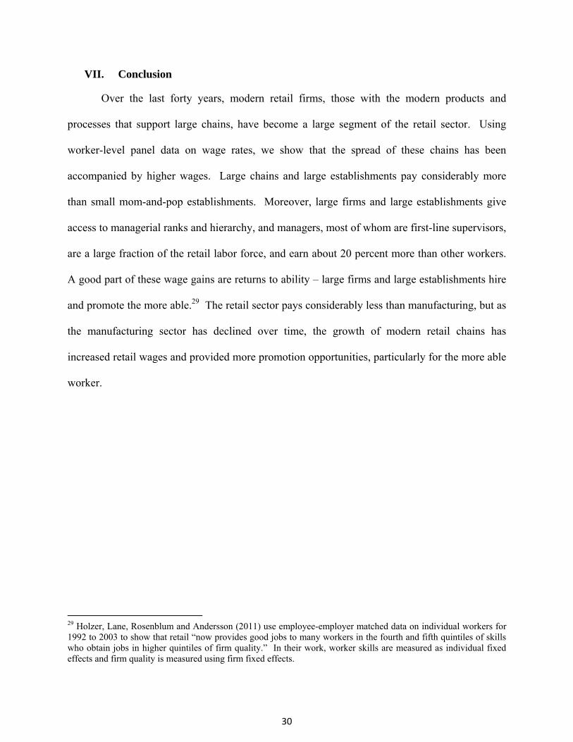
contrast between manufacturing and the retail sector is illustrated in Figure 1. This figure shows

that employment in the retail sector considerably exceeds that in manufacturing, and that it has

grown significantly over time, while employment in manufacturing has shrunk.

The goal of this paper is to examine the wages that accompany the spread of retail in the

economy. In particular, does retail trade pay only minimum wages, as some policy discussions,

and the intensity of competition in that sector, suggest that it might? Or, are there higher wages

for workers? Are the productivity gains associated with modern retail firms – as defined below

– accompanied by higher or still lower pay?

These questions are especially important because the retail sector is likely to continue to

flourish. Much of the economic activity in retail relates to non-tradable goods, so jobs here are

likely to stay. As in manufacturing, there is room in retail for substitution of computers for

people; but, contrary to manufacturing, overall growth in the sector so far is swamping that

                                                            1 More generally, Autor, Katz, and Kearney (2006 and 2008) and Autor and Dorn (2013) find evidence of polarization in the labor market, with middle income jobs becoming rarer while lower-paid and higher-paid jobs are both growing in numbers.

  3

substitution. There is some substitution in retail also from brick and mortar to the Internet, such

that some of the retail jobs are in distribution centers rather than stores. However, when talking

about all retail trade, including, for example, gas stations, automobile dealers, and grocery stores,

the Internet still stands at less than five percent of retail sales.2

The segment of retail that is growing most is what we refer to as modern retail. We

define modern retail firms as those that have successfully developed as regional or national

chains in the last few decades. Following Milgrom and Roberts (1990), modern retail firms are

perhaps better described as those that have undertaken product and/or process innovations.3 For

example, Wal-Mart is known for process innovations – for developing relationships with

suppliers and computerizing all elements of its supply chain. Many big retail firms have

followed Wal-Mart’s lead. Starbucks is known for product innovations – for making specialty

coffee a common retail good in the United States, and then exporting this concept globally.

Many large retail and service firms combine product and process innovations along with

organizational innovations.

There is ample evidence that the retail sector has become more concentrated, with

increasing numbers of large firms or chains that comprise modern retail. Foster, Haltiwanger

and Krizan (2006) report that the four-firm concentration ratio grew from 5.2% to 6.8% from

1987 to 1992. According to the most recent economic census, this ratio had reached 12.3% by

2007. Using data from the Economic Censuses and the Longitudinal Business Database (LBD),

Jarmin, Klimek, and Miranda (2009) also show that there has been an increase in firm and

establishment size in retail (see also Basker, Klimek, and Pham, 2012).

                                                            2 See http://www.census.gov/econ/estats/ for the latest statistics on this, which as of this writing, was for 2011. Note that the five percent above refers to the proportion of sales in Retail Trade (NAICS 44-45) only. 3 In other words, we refer to Modern Retail as the retail equivalent of Modern Manufacturing, which Milgrom and Roberts (1990) define based on a system of product and process innovations in manufacturing that is accompanied by a set of complementary organizational practices, like lean manufacturing.

  4

These increases in firm and establishment size may be promising developments for the

wage levels of employees in retail, for three reasons. First, there may be an increase in wages as

firms grow in size. Research has provided strong evidence of positive firm-size effects on wages

in the economy as a whole, after controlling for work conditions and worker quality.4 Second,

there may be an increase in wages for larger establishments. Many big box chain stores are large

establishments compared to the more traditional mom-and-pop store. Third, relative to

traditional mom-and-pop stores, there is more room for promotion to supervisor or manager in

large firms, and with such promotions come the promise of higher wages. Firm size,

establishment size, and promotion are the determinants of wage levels that are considered in this

paper.

We model wage levels using data from the 1996 to 2013 Current Population Survey

(CPS) and the National Longitudinal Survey of Youth (NLSY) from 1986 to 2010. The CPS

data provide the large sample size needed to model wage levels as a function of firm size. The

NLSY data provide the longitudinal platform to model the determinants of wages and to estimate

establishment size effects.

At the end of the analysis, wages in the retail sector are compared to wages in

manufacturing. The reasons for this comparison are twofold. First, the presence of high-paying

jobs in other sectors, including manufacturing, is often attributed to the presence of rents that are

then shared with labor. The retail sector, in contrast, is typically viewed as very competitive,

leaving little scope for such rent sharing. Second, there is an emphasis on “good jobs” in

manufacturing in the public discourse, with the implication that policies should be put in place to

                                                            4 See Brown and Medoff (1998), Oi and Idson (1999), Fox (2009), and Pedace (2010). Bayard and Troske (1999) analyze a cross section of data in the retail industry from 1990 and find no firm-size effects on wages using a linear model of firm size. They do find establishment size effects.

  5

try to restore the predominance of manufacturing in the economy. It is, therefore, natural to ask

how much retail differs from manufacturing, or, if there are any similarities.

The results are as follows:

1. Wage rates in the retail sector rise markedly with firm size and with establishment size.

Holding constant a set of standard control variables, pay is 15 percent higher in large

firms (1000+ workers) compared to small (less than ten workers) for the high school

educated. For those with some college education or a degree, pay is 25 percent higher in

large than small firms. Across establishments, pay is 26 percent higher for large

establishments (500+ workers) versus small (less than ten workers) for those with high

school education, and 36 percent higher for those with some or more college education.

2. When we control for unobserved worker quality, firm and establishment size premia

decline markedly. Adding worker fixed effects to wage regressions, when a worker

moves from a small firm to a large firm, his pay rises by 11 percent for the high school

educated and 9 percent for those with some college education or college degree. When a

worker moves from a small establishment to a large one, pay rises by 19 percent for high

school educated and by 28 percent for those with some college education.

3. Taken together, these regression results imply that higher quality workers are sorted into

large firms and large establishments, but that working in larger firms or establishments

yields additional increases in pay.

4. Higher quality workers are also sorted into managerial positions. Comparing pay across

workers of different ability levels, managers earn more than 23 percent more than non-

managers if they are high school educated, and 20 percent if they have some college

education or more (using CPS data). Holding constant worker ability via worker fixed

  6

effects, promotion to a management job increases pay by 8 and 7 percent for these two

educational groups. Moreover, the proportion of individuals that are promoted to

manager is high, at 28 percent, in retail.

These pay increases with firm size and establishment size and with managerial

occupation are treatment of the treated effects – these are the pay increases that would be

received conditional on obtaining a job at a large firm or establishment or as a manager. That is,

the estimated wage return to promotion is conditional on being promoted to manager, which may

require special skills, like organizational skills or people management skills.

In sum, the increasing firm size and establishment size that are a hallmark of modern

retail are accompanied by increasing wages and opportunities for promotion for many workers.

While retail pay is considerably below that in manufacturing, pay in retail is above that found in

service jobs, as defined by Autor and Dorn (2013). The results below contradict the image of the

retail sector as one comprised of the lowest paying jobs in the economy.

I. The Rise of Modern Retail

The growth of the retail sector has been accompanied by growth in modern retail chains.

Over the last several decades, the growth in firm size in the retail sector has been pronounced.

Foster, Haltiwanger and Krizan (2006) and Jarmin, Klimek, and Miranda (2009) document the

growth of large chains and rise of modern retail. Modern retail calls to mind chains like Wal-

Mart and Home Depot, but the trend towards large-scale retail firms predates these. Jarmin,

Klimek, and Miranda (2009, p. 237) point out that single-location retail firms accounted for 70.4

percent of sales in 1948, but only 39 percent by 1997. Similarly, over this time period the

market share of sales accounted for by firms with more than 100 establishments rose from 12.3

percent to 36.9 percent (p. 238). Using data from a 1971 Census Bureau report and information

  7

they compiled from the Longitudinal Business Database, they show that retail establishments

operated by multiple-establishment retail chains accounted for only 20.2 percent of all

establishments in 1963, but reached 35 percent by 2000. As a result of the growth of chains,

employment at single-location retailers grew by 2 million between 1976 and 2000, but

employment at chains grew by 8 million.

One source of rising demand for retail chains has been the rise of women in the work

force (Pashigan and Bowen, 1994). Women’s increasing income and resulting time constraints

have led to an increase in the demand for branded products, because brands convey information

that otherwise takes time to assess. Nationally recognized brands save shopping and search time.

The growth of retail chains has been accompanied by growth in retail establishment size

as well. Between 1958 and 2000, the average retail establishment went from about six to more

than fourteen workers (Jarmin, Klimek, and Miranda, 2009, page 240 and Figure 6.4). This

growth in establishment size has been especially pronounced in chains. From 1976 to 2000,

small mom-and-pop stores grew from 5 to 7 employees per store. In the same period, local chain

stores increased their number of employees from 9 to 15, regional chains from 12 to 15, and

national chains from 15 to 25 (Jarmin, Klimek, and Miranda, 2005). Holmes (2001) argues that

this tendency is the result of the important investments in technologies, such as barcodes and

related inventory management techniques, that retail chains can make. Similarly, Basker,

Klimek, and Pham (2012) discuss how the breadth of products sold in the typical store of a chain

store has increased with the number of establishments in the chains. They explain this as the

interaction between technological advances and associated scale and scope economies, along

with consumer desire for one-stop shopping.

  8

Productivity growth in the retail sector has been enhanced markedly by the growth of

chains. Foster, Haltiwanger, and Krizan (2006) show that the net entry of establishments

accounts for most of the productivity growth in the retail sector over time, and that this net entry

is driven by chain stores. Productivity gains in modern retail are due to investments in

information technologies that lead to lower inventories, more frequent deliveries, and larger

stores (Jarmin, Klimek, and Miranda, 2009; Holmes, 2001). Given these mechanisms for

productivity growth, one would expect that large chains would have the greatest productivity

gains from information technologies. And indeed they do (Doms, Jarmin, and Klimek, 2004).

The retail sector has contributed to overall productivity growth in the economy over the last 50

years. Jorgenson, Ho and Samuels (2011) state that when they order industries by contributions

to value added and productivity, wholesale and retail trade are heading the list.5

As the numbers above indicate, mom-and-pop stores (which we equate to single-location

stores) have not become extinct with the growth of large chains. On the contrary, large numbers

of these stores continue to offer a variety of products, including many specialty products. While

these are stores where productivity is unlikely to grow much due to information technologies,

workers may be more highly skilled as they sell these speciality products.

How does the growth in productivity in modern chains affect labor demand in the retail

sector? Autor, Levy, and Murnane (2003) show that within industries, non-routine analytic and

non-routine interactive tasks exhibited strong growth in employment throughout the 1970s to

1990s. In contrast, routine cognitive and routine manual tasks have experienced declines. How

might these overall trends apply to retail trade? Autor and Dorn (2013) cite cashiers as an

occupation ranked high on the Routine Task Index, suggesting that employment of cashiers is

                                                            5 Conversely, Haskel and Sadun (2011) show that regulation in the U.K. retail sector has led to smaller shops and a total factor productivity slowdown.

  9

reduced due to the substitution of capital for routine tasks. Basker (2012) examines the effect of

the introduction of scanners in grocery stores. Much of retail trade has adopted bar code

scanners that raise productivity. Smart cash registers, using pictures, also substitute for labor in

the fast food and restaurant industries. So there has been some substitution of capital for labor.

Autor, Levy, and Murnane show that the industries that invest in information technologies –

which would include scanners and cash registers – have lower demand for labor performing

routine work. Retail contains a mixture of routine and non-routine work according to their

definitions. And the evidence from Basker (2012) suggests that scanners did increase

productivity in the supermarket industry by reducing payroll. However, the job growth in retail

overall implies that the increased demand for retail output has more than outpaced any reduction

in labor demand arising from increased reliance on technology.

II. Wages in Retail: Evidence from Case Studies

Before turning to the analysis of wages using survey data, it is valuable to look to case

study evidence on pay in some well-known firms. Table 1 summarizes data from Glassdoor on

pay at Wal-Mart, Starbucks, Whole Foods, and Costco.6 These cases demonstrate that not all

retail work is low paying. In these firms, on average, even cashier pay is above the current

federal minimum wage. But what is most pronounced is the increase in pay for workers who

become managers. According to these data, an entry level cashier in a Wal-Mart store earns

$8.48 per hour, but a Supervisor earns $14.38 per hour. Turning to jobs that are salaried, pay

rises: a Shift Manager earns $62,837 and a Store Manager earns $92,462. Wal-Mart is at the

mid-point of our set of cases. Starbucks pays less; its establishments are smaller. The high-end

grocery and big-box stores, of Whole Foods and Costco, pay higher wages. While these are but

a few examples, they illustrate well some of the overall patterns revealed in the analyses below.                                                             6 Glassdoor.com is a website where people voluntarily enter their wages and jobs. The site then publishes averages.

  10

These patterns are also evident at the bottom of Table 1, where mean wages using Current

Population Survey data are displayed.

III. Data Sets

The retail sector that is the focus of this study is the one that the “man on the street” or

the press would consider retail. It combines two broad industries per the North American

Industry Classification System (NAICS), namely the Retail Trade and the Accommodations and

Food Services – respectively 15 million workers and 12 million workers according to the BLS by

the end of our data period – as well as some segments of the Automotive and Repair Services

industry, the Arts, Entertainment and Recreation industry, and the Personal Services sector. See

Appendix A for details. We combine these, and refer to the combination as the Retail sector,

because the notion of the labor market being dominated by low paying jobs relates to the growth

in the combination of all these sectors. This broad definition also aligns better with the SIC

(Standard Industrial Classification) definition of the retail sector which was used by the Census

Bureau until 1997, which included in particular “Eating and Drinking Places.”

Data from the 1996 to 2013 March Supplement of the Current Population Survey (CPS)

are used to model retail and manufacturing wage levels and employment. The CPS measures

firm size by asking respondents to state how many people work at all locations of their employer.

Yearly income, occupation, industry, and firm size all refer to the respondent’s longest job in the

previous year, and thus 2012 income is the most current available (reported in the 2013 survey).

The sample begins with the 1996 survey because there was a major change in sampling frame for

the CPS in 1996. For the OLS regressions below, our CPS sample for retail includes 234,667

observations, or individual-years, covering 194,581 unique individuals ages 18 to 64 (see Table

2). For manufacturing, the same database yields a sample of 179,550 individual-years, for

  11

139,499 unique individuals in the same age range. The subsample of individuals that we can

track over two time periods, and where the individual remains in retail or in manufacturing for

the two years, is relatively small compared to the overall sample, with 40,086 individuals in

retail and 40,051 individuals in manufacturing.7 There are many reasons for this relatively low

match rate. First, only half the observations for the first and last year in the data (1996 and 2013)

can be matched within our data as the other half match with out-of-sample observations. For the

other years, due to factors such as migration, mortality, non-responses, etc., the maximum

matching rate is estimated to be about 70% (see Madrian and Lefgren, 1999). Moreover, for our

purposes, we restrict the sample to those individuals who are within the right age range in both

years, work full time in both years, and are in retail or manufacturing in both years.

The definitions of all the variables used, along with descriptive statistics calculated with

relevant sampling weights, are show in Table 2.

Data from the National Longitudinal Survey of Youth (NLSY) are used to complement

the CPS data. The data from the NLSY follows a panel of respondents who were 14 to 22 in

1979 when the panel began, extending to 2010. In 1986, the NLSY began asking respondents

about the size of the establishment in which they work. Using the panel nature of the data, the

effects of establishment size can be modelled with controls for worker fixed effects. Therefore,

the regressions below use data on respondents aged 21 to 53 from 1986 through to 2010, with

odd-numbered years skipped after 1994 because the survey was not conducted in those years.

There is oversampling of the economically disadvantaged in this database, and our regression

results below reflect this fact. There are 17,914 individual-year observations in the retail sector

and 19,029 individual-years in manufacturing, for a total of 4,904 and 4,218 individuals,

                                                            7 Matching is done as prescribed in the Census Department’s “How To Link CPS Public Use Data Files,” available at: http://www.census.gov/cps/files/How%20To%20Link%20CPS%20Public%20Use%20Files.pdf.

  12

respectively. Due to attrition in the sample, and movements in and out of the labor force, and in

and out of the retail and manufacturing sectors, we observe an average of three to four years of

data for each person in each sector. The means of the variables of interest, calculated with

appropriate sampling weights to represent population estimates, as well as all variable

definitions, also are shown in Table 2.

The descriptive statistics in Table 2 and the regressions below use only the data on full-

time workers, or those working 35 or more hours per week, the standard definition used by the

Bureau of Labor Statistics. The retail sector is one that comprises a large number of part-time

workers. In the CPS data, in retail, 70 percent of employees are full time, with 61 percent of

women and 78 percent of men working full time. In manufacturing, the comparable numbers are

much larger, at 95 percent for all employees, and 91 percent and 97 percent for women and men

employees respectively. Our goal is to model pay for those whose primary job is in retail, and

who dedicate most of their time to that job. Nonetheless, for comparison purposes, we show in

Table A1, in the appendix, the same information as in Table 2, but for samples that include part-

time workers. Though not shown, when we add part-time workers to our regressions below,

some magnitudes differ but conclusions are unaffected.8

IV. Some Simple Statistics

There are some surprises in the mean wages and characteristics of workers that one

garners from the descriptive statistics in Table 2 (and Table A1). First, retail is not comprised

only of less educated workers. In the CPS data, only 52 percent of fulltime workers in retail

have a high school education or less, with the vast majority of those having completed high

school. For those with more than a high school degree, 31 percent have some college, and 17

percent have a college education or more. The level of education of workers in both retail and                                                             8 An appendix showing results when part-time workers are included in all our analyses is available upon request.

  13

manufacturing has gone up over time. Though not shown in the table, the data show that in retail,

the average years of education rose modestly from 12.6 to 13 between 1996 and 2013, while in

manufacturing, years of education went from the same 12.7 to 13.4 on average over this period.

The proportion of individuals with more than a high-school education (i.e. more than 12 years of

education) increased from 43 percent to 51 percent in small retail firms (499 or fewer

employees) and from 46 to 56 percent in large retail firms (500 or more employees).

Second, there is a very large number of managers: 28 percent of full-time retail workers

self report that they are managers, as compared to 19 percent in manufacturing.9 Note that 18

percent of the full-time labor force in retail are first-line supervisors who are managing shifts of

workers. In other words, in retail, 64 percent (.180/.288) of all managers (as we define managers)

are first-line supervisors. Thus what we traditionally think of as managers (more senior than

first-line supervisors) are 10 percent of the full-time workforce. We have been very careful to

include the first-line supervisors, erring on the side of having too many managers. For example,

a “chef” in a restaurant is designated a manager because a large percent of his time is spent

managing others. Combining these first-line supervisors with managers from headquarters, the

percent manager gets quite high. If we look at the entire retail workforce, including part-time

workers, the percent manager in retail falls to 22 percent, while it is virtually unchanged in

manufacturing, at 18 instead of 19 percent (see Table A1, in the Appendix).

Third, the distribution of employment by firm size and establishment size is quite

dispersed. Large firms employ a large number of people: similar to manufacturing, where large

firms account for 44 percent of employment, 41 percent of fulltime employment in retail is in

                                                            9 Abraham and Spletzer (2007) show that the percent manager reported in the CPS is considerably higher than that reported by a survey of firms in the BLS OES (Occupational Employment Statistics) data for 1996-2004. Some of the difference can be explained by how “managers” are coded in the OES, but even after correcting manager definitions in the OES, a significant and unexplained discrepancy remains. The NLSY does not contain information allowing us to identify first-line supervisors separately from managers before 2002.

  14

firms with more than a thousand employees. But mom-and-pop firms and establishments are

still prevalent in retail: Firms with less than ten employees account for 18 percent of employment

and those with less than 100 employ 45 percent of the retail labor force, i.e. they account for as

many employees in this sector as large firms do. Moreover, establishments with less than 10

employees are 32 percent of employment in this sector.10

Another feature of retail, not displayed in Table 2, is that the number of people employed

by large retail firms and large retail establishments has grown over time. Those employed in

large firms (of 500+ employees) grew from 42 percent to 47 percent in the retail sector, and

those in large establishments (50 or more employees) grew from 33 to 52 percent. In contrast to

retail, in manufacturing, there was no change, or even perhaps a slight decrease, in the percent

employed by large firms, and also no change in the percent working in large establishments.11

Retail is noteworthy also because it provides substantial employment for women. From

the CPS data, only 30 percent of manufacturing workers were women during the period of our

data; in retail, even among those working full time, this figure was 44 percent. Thus, the decline

in the number of jobs in manufacturing shown in Figure 1 pertains more to men as they

predominantly occupy these jobs. Moreover, larger firms in retail employ a greater share of

women workers. Fifty percent of employees in firms with 500 or more employees are women,

whereas for firms with fewer than 500 employees, this proportion is only 39 percent. Both of                                                             10 We used the Census of Retail in 2007 to check some of these numbers, based on self-reports, against those reported by firms in the Census. Using the definition of retail from the Census, i.e. NAICS 44-45, and restricting our sample to year 2007 data, our breakdown of employees on the payroll by firm size is: Size<10, 14.3 percent for the CPS, 10.8 in Census; Size10-99, 21.2 percent in the CPS, 20.2 percent in the Census; Size100-499, 9.6 and 8.0; Size500-999, 4.6 and 2.4; Size1000+, 50.3 versus 58.6. With this definition of retail, the breakdown of employees by establishment size in 2007 is: Estab<10, 22.0 percent for the NLSY versus 18.1 percent in Census; Estab10-49, 25.9 percent for the NLSY, 33.5 percent for Census, Estab 50-99, 17.1 percent for the NLSY and 14.8 percent for the Census, and for Estab100+, we have 35.1 percent versus 33.6 percent in Census. 11 An alternative way to show the same data pattern is to note that the average firm size in retail in the CPS data has grown steadily from 639 employees in 1995 to 725 in 2012. In manufacturing, in contrast, the average size was 797 in 1995 and 799 by 2012, having grown a bit in the late 90s but shrunk through most of the 00s only to bounce back in the last few years. To compute these averages, firm size is measured as the midpoint of each range shown in Table 2, with those in firm size 1000+ given a size of 1500.

  15

these proportions, moreover, have remained basically the same over the whole period covered by

our data. In manufacturing, this proportion is 30 percent on average over the period of our data

for both smaller and larger firms. As for differences across establishment size categories in retail,

they are less pronounced: 46 percent of employees of larger retail establishments (≥ 150

employees) are women, compared to 42 percent in smaller establishments.

The data in Table 1 above suggest considerable variance of pay in retail, variance that is

often unacknowledged in popular discourse about wages in the sector. Figure 2 shows this

variance using the CPS and total wages and salaries for the previous year for those that work full

time. In 2010 dollars, 34 percent of non-managers earned less than $20,000 annually, but at the

high end of the spectrum, 13 percent of non-managers earned $50,000 or more.12 For managers

in retail, the pay is higher, not surprisingly, but also even more dispersed: 13 percent earn

$20,000 or less, while 33 percent earn more than $50,000.

Retail wage rates are compared to wages for two alternative sets of jobs, those in

manufacturing, and those in service occupations. In the CPS data, retail workers earn 68 percent

($16.64 / 24.33) of what manufacturing workers earn. Regressions below explore differences in

retail and manufacturing in the wage premia for firm size and for management status.

The second comparison of interest is the mean wages in retail relative to service

occupations. As defined by Autor and Dorn (2013), a service occupation is one that offers

personal services, such as a gardener, housekeeper, or nanny.13 Do retail jobs pay as little as

service occupations? There are two reasons to ask this question. The first is that service jobs are

considered to be the typical job encountered by low-skill workers. The second reason service

                                                            12 For the figures, we do not weight the data. As a result, there are 5 additional observations in this sample, i.e. there are 5 observations in the retail sample that receive weights of zero per the CPS. Also, for Figure 2, we include only workers who indicate that they worked most of the year, defined as 40 weeks or more in the prior year. 13 Note that this is a discussion of service occupations (e.g. nannies, gardeners, cosmetologists, etc.) found mostly in the personal services sector. See the Appendix for a list of occupations included in this group.

  16

occupations are of interest is that they have been growing in numbers while middle income

occupations – such as those in manufacturing – decline. Service occupations are rarely

computerized, and so the quantity of these jobs and their pay has risen over time while middle-

income routine work has been squeezed out due to computerization (Autor and Dorn, 2013).14

Using CPS data, we find that service occupations paid $13.97 and $11.15 for men and women

respectively, while retail occupations paid $16.28 and $12.79, respectively. Thus, retail jobs pay

16.5 percent (men) to 14.7 percent (women) more than service jobs do.

In sum, when we think of retail, we should think of a growth sector with some

computerization that pays 16.5 percent more for men and 14.7 percent more for women than

jobs in service occupations. In other words, wage rates in retail are sandwiched between those in

manufacturing and those in service occupations.

V. Wage Regressions

The rise of modern retail firms brings to mind images of hamburger flippers and sales

people earning minimum wages in impersonal stores at the expense of traditional retail jobs in

mom-and-pop restaurants and shops. However, there are at least two features of modern retail

firms that, in our view, should alter this image. First, modern retail firms are big. As described

above, retail chains are typically either regional in nature – suggesting mid-size firms – or

national or even international in scope – suggesting very large firms. In our data, 41 percent of

full-time workers in retail work in firms of more than 1000 workers (Table 2). If wages rise with

firm size on average, the growth in large firms will improve retail wages. Second, because

modern retail firms are bigger, they have more layers of management. More managers earning

                                                            14 Autor and Dorn (2013) provide little information regarding where retail jobs fall in the spectrum of wage polarization because their analysis aggregates retail jobs with clerical jobs.

  17

pay that exceeds entry level pay improves retail wages as a whole. Both these effects are found

in the wage data. The relevant evidence is contained in the subsections below.

A series of wage regressions are estimated to identify the wage returns to firm size,

establishment size, and managerial status. These regressions are:

(1) lnWageit = Sizeit + Managerit + Xit + i + it

where Size is a categorical measure of firm size (for CPS) or establishment size (for NLSY),

Manager is a dummy variable for managerial occupation, including first-line supervisors, X is a

vector of control variables that includes education, experience, and dummy variables for married,

Black, and for living in an urban area. Because the CPS data do not include a measure of work

experience, experience is calculated as age minus education minus six. Since women are more

likely to be out of the labor force for periods of time, this measure is likely to overestimate the

experience of women more than that of men. For the NLSY data, our measure of experience is

the cumulative number of years as calculated from reported weeks per year times average hours

per week in the data. Thus our measure of experience in the NLSY does not overestimate the

work experience of women while that in the CPS will tend to do so.

The regressions are estimated with and without worker fixed effects, i. The aim of the

regressions is as follows. The first set of regressions are OLS, with standard control variables

listed above. The goal is to estimate treatment effects – of moving to big firms or managerial

jobs – with some standard controls for worker quality. Because workers who are better educated

are more likely to be hired by large firms and more likely to become managers, it is important to

control for worker characteristics - observed and unobserved - when estimating these effects.

The second set of regressions thus control for worker fixed effects. These regressions hold

constant unobserved worker ability, i, that can produce omitted variable bias in OLS estimates

  18

of the incremental returns to firm size. If the OLS coefficients on firm size exceed the fixed

effects coefficients, the difference measures the degree to which there is sorting of good workers

to large firms or managerial positions based on workers’ unobserved characteristics.

The coefficients on Size and on Manager are estimating treatment of the treated effects,

not average treatment effects. In other words, there are additional relationships that would pick

up the sorting of workers into the Size and Manager categories. For example, for the size effects,

big firms or big stores may have a larger queue of workers from which to choose and may be

more careful in their selection of workers, or they may be less likely to choose workers who

might be considered risky, or they may hire based on personal referrals. Alternatively, workers

with certain character traits (e.g., those who like to interact with more colleagues, or who are

more risk averse) may be attracted to, and seek jobs in, larger firms or establishments. In either

case, the coefficient on Size in (1) represents the treatment of the treated because it captures the

effect of Size on the wages of the workers who are hired by big firms or big establishments.

Whether the treatment of the treated effect would be larger or smaller than the average treatment

effect depends on this sorting of workers to firms. Similarly, and perhaps more realistically, there

is a set of variables that would cause workers to be promoted to manager. Those promoted may

be better organized, have better people skills, or instill trust in others. The coefficient on

Manager in (1) is the treatment of the treated because it represents the effect of Manager on the

wages of workers who are selected to be managers because they have these traits. There is no

data on which to estimate average treatment effects because movement to large firms or to

managerial occupations is never imposed randomly on workers.

A. The Effects of Firm Size

There is an abiding interest in whether the retail sector provides “good jobs” for those

  19

who are less educated. Therefore, a natural question to ask is, how do the less educated fare in

retail? Do the less educated earn more at large firms or as managers, or is all the increase in

earnings power from moving to larger retail chains conferred on better educated retail workers?

Table 3 answers these questions using CPS data from 1996 to 2012. In Table 3, we show results

first for the largest sample available in the CPS for two educational groups, those with high

school or less (column 1), and those with some college or more (column 2). We do this so we

can assess how well those with low education fare in retail. We then show OLS (columns 3 and

4) and then fixed effects results (columns 5 and 6) for the sample of individuals for which we

have repeat observations so we can compare the OLS and fixed effects results on the same

sample.

Large retail firms pay more than small firms in the retail sector if an employee has a

high-school or less education, but they pay considerably more for those with some college

education or more. From Table 3, for the high school educated, a firm with 100 to 499 workers

pays 20.9 percent more than a small firm with less than 10 workers. Note that this is not a

manager effect, as we control directly for manager status. For the worker with some college

education or more, the larger firm pays 30.1 percent more.

Pay does not rise linearly with firm size. There is an immediate bump up in pay when

moving from small (less than 10) to slightly larger (10 through 99) and then to mid-size firms

(100-499). The best-paid jobs are those in firms with 100-499 workers across both education

levels although the next size up involves wages that are not statistically lower. These high-

paying firms may be regional chains, and/or chains comprised of unionized stores.

Higher pay in larger firms might arise if larger firms hire workers who are more skilled.

Regression results support this hypothesis. Introducing worker fixed effects in Columns 5 and 6

  20

shows that the returns to firm size fall considerably when controlling for worker’s unobserved

ability—firm size effects are about one-half to one-third as big, depending on the education

group. Recall that in the CPS data, identification of firm size effects in fixed effects regressions

comes from only a one-year change in wages as workers move between firms. Still, in all

instances, a comparison of the OLS results (in columns 3 and 4, which use the same sample as

the fixed effects regressions) to the fixed effects results (in columns 5 and 6) suggests that there

is a sorting of better workers to larger, better-paying firms.15 Workers selected by large firms

may differ in some unobserved ways from those who are not.16 The subset of those selected by

large firms benefit from higher pay.

Why do larger firms pay higher wages than small? Pay premia in larger firms have long

been a puzzle in economics, just as it has been a stable result across data sets and time periods.17

Part of the story is that big firms are hiring higher quality workers; the fixed effects results show

this. But a sizeable wage premia remains after controlling for worker fixed effects. It may be

that big firms are offering compensating differentials for more onerous work, such as more

nighttime hours in big stores than in mom-and-pop stores. We do not have data on nighttime

hours to test those possibilities. But we compare workers in businesses that sell merchandise to

workers in the restaurant sector, where the latter are especially likely to have to work nights, and

find very similar patterns of firm and establishment size wage premia. The fact that we find these

                                                            15 Wage growth regressions validate this finding, but also confirm that firm size and promotion effects remain after we control for unobserved worker ability. For example, using the CPS data, wage growth regressions indicate that moving from a firm with fewer than 10 workers to a larger one is associated with an increase of 7.2 percent in wages for the high-school educated, and 8.3 percent for those with some college education or more when we control for changes in Manager, Education, Experience, Married, and Urban. Similarly, a movement to manager is associated with an increase in pay of 8.2 percent for those with a high-school degree or less, and 6.6 percent for those with some college education or more. 16 Fox (2009) shows that the firm size wage premium increases with the level of worker responsibility on the job, where responsibility means advancing in the job to supervise others. This could imply that large firms will look for workers who can shoulder more responsibility. 17 See footnotes 4 and 16 above.

  21

wage premia even in narrowly defined sectors, such as within the restaurant industry, moreover

suggests that wage premia are not due to inter-industry differences. It may be that workers in

large stores work harder. This could be due to efficiency wages – that offering higher wages will

induce higher effort. We checked to see if the firm size effect has changed over the 17 years of

our data, and it has not. The puzzle largely remains. The most likely explanation in our view is

that employees in larger firms are more productive on average – due to technology investments,

intangible assets such as brands, increased coordination, and so on, and that they are

compensated for their increased productivity or simply able to share in the increased returns

generated by these technologies and intangible assets.

B. The Effects of Establishment Size

Major retail chains are typically larger firms; they are also typically, though not always,

comprised of larger establishments. As described above, big box stores have more employees

per store than the typical mom-and-pop stores. Of course, the correlation between firm size and

establishment size is far from perfect – many big chains, like fast-food and other restaurant

chains, have fewer employees per store than would a standard grocery store or a traditional

department store.18 But if large stores are becoming more common, as described in section I

above, the question is, do larger establishments pay higher wages like larger firms do?

Wage levels rise markedly with establishment size according to the NLSY data (Table 4),

across both educational levels. Working in a store with 500+ employees pays 26 percent more

for high-school educated and 36 percent more for those with some college education (including

those with a college degree or more), relative to working in a store with less than 10 employees.

                                                            18 We are unable to assess this correlation in our data since the CPS includes information on firm size only, and the NLSY includes information on establishment size only.

  22

For both education levels, the effect of store size rises steadily as we move from stores with less

than 10 employees through to the larger size stores.

Here as well, some portion of the wage gain as store size increases is a return to workers’

unobserved ability. When worker fixed effects are introduced in the regressions, the gains to

store size remain, but for those with a high-school or less education, they fall twenty-some to

thirty-some percent across establishment sizes. For those with more education, we see such a

reduction only in the largest establishments. The NLSY data has three to four observations per

person on average in retail, from which to estimate the store size effects while controlling for

worker fixed effects.

Why do larger establishments pay higher wages than small ones? The potential

explanations are the same as those for the firm size effects discussed above. Yet again, we find

no time-series changes in premia. We also find no difference in premia for rural versus urban

markets. The latter result is especially interesting as establishments in rural areas are those that

would be most likely to benefit from market – specifically monopsony – power in their local

labor markets, which would suggest lower wage premia in rural markets. But we find no

evidence of such differences. We also find sizable establishment size effects within the restaurant

sector and within merchandise retailing. Thus inter-industry differences do not seem to be the

source of the establishment size differences that give rise to the wage premia. Again, it may

simply be that employees in larger retail establishments are more productive – due to selection or

the productivity benefits of larger establishments – than those in smaller establishments, on

average.

C. Promotions

One of the key features of modern retail firms is that promotion to managerial positions

  23

provide opportunities for pay increases. Darden Restaurants states that “More than half of our

restaurant managers are promoted from hourly positions,.., and nearly 100 percent of general

managers and managing partners are internal pomotions.”19

Managers in retail in the CPS and NLSY data are predominately lower-level supervisors.

In selecting the occupational codes to define managers, we purposely selected managerial

occupations to include those who are first-line supervisors (see Appendix). The majority of the

managers in the data are therefore low level, not high-level management. Recall that from Table

2, 64 percent of the people who are managers in the CPS data are, indeed, first-line supervisors.20

It is, however, true that well-educated workers are much more likely to be managers. The

percent manager rises from 22 percent for high-school educated or less to 35.5 percent for those

with some college or more (CPS data, full-time workers). Note that by running wage regressions

within educational group, we control for the degree to which the wage gains for managers are

due to sorting by educational group.

The effect of becoming a manager on wages in retail can be estimated in both the CPS

data and the NLSY data. The regression results show that manager effects on wages are sizable

in the two data sets. Wage rates are 22.6 and 15.3 percent higher for high school educated

managers, all else constant, in the CPS and NLSY data (Tables 3 and 4). The gains are similar

for the workers with some college or more – at 19.5 and 16.1 percent respectively. Because

managers are better educated, when education is dropped from the regression (not shown), the

estimated returns to being a manager become larger.

Managers who work in large stores earn more than those who work in small stores.

While not displayed in Table 3, we estimate regressions with interactions between the Manager

                                                            19 Jennings (2013). Darden is the owner of eight restaurant brands, including Olive Garden and Red Lobster. 20 The NLSY does not include codes to identify supervisors separately from managers prior to 2002.

  24

dummy variable and store size.21 For the high school educated, a manager in a small store (Size

<10) earns 12.6 percent more than a non-manager. But managers in all bigger stores earn wage

premia that are about twice that. For example, a high-school educated manager in a store of Size

100-499 earns 28.2 percent more than a non-manager. Results are comparable for the college

educated.

A sizable portion of the wage increase that accompanies a promotion to a managerial

position is a return to ability. In worker fixed-effects regressions with the CPS data, movement

into management raises wages by only 8.3 percent and 6.5 percent for each education group

(Table 3). Similarly, in the NLSY fixed effects regressions, the movement into management

increases wages by 10 percent and 8 percent, respectively, for the two education groups (Table

4). These pay premia for managerial skills are treatment of the treated results. Managers’ pay

may reflect unobserved skills – like organizational skills or people skills – that are rewarded with

higher pay when a worker is promoted to manager status.

D. Worker Sorting

Taken together, the wage regressions above show that there is sorting of higher quality

workers into big firms, big establishments and managerial occupations. Looking across the

numerous regressions in Tables 3 and 4, the wage gains for firm size and for establishment size

fall considerably when comparing the OLS estimates of these effects to the worker fixed effects

estimates (in Table 3 for the CPS data and in Table 4 for the NLSY data). Nonetheless, working

in a larger firm, and/or a larger establishment, and getting promoted to a managerial position still

benefits the individual worker beyond what is necessary to compensate for unobserved ability.

                                                            21 Results from these regressions are available upon request.

  25

E. Gender Gap

Women represent almost half of the full-time labor force in retail (Table 2). This might

lead to an expectation that the retail gender wage gap would be low, and that women would be

promoted to managerial positions with greater frequency in this sector. Holding constant firm

size and all other variables, wages are 25 and 21 percent lower for women in the CPS data, for

high school educated and those with some college or more (Table 3). The gender wage gap is the

same in the NLSY data (Table 4).

These regressions do not control for the detailed occupations of women and men.

Women may be cashiers and men forklift operators. However, if we estimate the wage

regressions within a major occupational category – that of cashiers – in the CPS data the pay

received by women remains 17 and 20 percent lower, respectively for the two education levels,

all else constant in the regression (not shown). Nevertheless, these regressions do not tell us that

firms are paying differential amounts for like workers. The mean values of Table 1 show that if

women choose to work at Starbucks and men choose to work at Costco, men will make

considerably more than women.22

We delve deeper into the pay differences for men and women by estimating wage

regressions by gender. In OLS, the gains to firm size and managerial status are similar for men

and women (Table 5). The gains to establishment size are greater for women than men (Table

                                                            22 Neumark (1996) conducted an audit study of restaurant hiring. In that study, he sent women and men with identical resumes to high priced restaurants that pay higher wages than average restaurants. He found that women are less likely to be interviewed and less likely to be hired than men. There is some evidence that it was due to customer discrimination. The implication is that high-paying restaurants are less likely to hire women than men: women are more likely to work in low-paying restaurants. Neumark’s study is now twenty years old and did not measure whether women are less likely to apply to work at higher paying restaurants. Still, in a more recent similar study aimed at science recruiting, Moss-Racusin et al (2012) found that identical resumes for men and women graduate students applying for lab manager positions received different salary and mentoring offers.

  26

6).23 Combined with results on the wage gap, these results imply that base pay is lower for

women than men, the rate at which pay grows with firm size or managerial promotion is similar

across the two genders, but women benefit particularly from working in larger establishments.24

As before, much of the wage premia with rising firm size is a return to ability for both

women and men. When worker fixed effects are added to the regressions, the returns to firm size

drop (columns 5 and 6, Table 5). There is less sorting of high-ability women and men across

establishments of different sizes: the fixed effects results (columns 3 and 4, Table 6) show wage

premia for big establishments that are pronounced, and statistically significantly greater for

women than men.

F. Education and Experience

While the popular press suggests that all retail jobs are low skilled, the estimated returns

to education in our regressions indicate otherwise. Tables 5 and 6 show the rate of return to

years of education, by gender. Without controlling for unobserved ability, the return to

education is 8.1 percent and 7.4 percent per year of education for women and men according to

the CPS data (columns 1 and 2 of Table 5), or 8.3 and 7.0 if we reduce the sample to be

comparable to that used in the fixed effects regressions. Similarly, the return to education is 5.8

and 5.4 percent for women and men in the NLSY data (columns 1 and 2 of Table 6). These

effects are again much smaller when we control for worker unobserved ability via fixed effects.

However, such estimation relies on very limited data, namely increases in education between two

years in the CPS data, and increases in education that occur almost exclusively in the early years

                                                            23 We also pool the samples for men and women to do t-tests of whether there are significant differences for the genders. In the CPS data, women earn 5 percent more than men in the Size1000+ size, and in the NLSY data, women earn significantly more than men across all the size categories relative to small establishments. 24 When we look at all workers, part-time and full-time, the regressions are very similar to those for full-time. The returns to firm size and establishment size are slightly lower for all workers. These results are available upon request.

  27

of the NLSY data. Note that the more educated also have bigger returns to firm size than the less

educated: in Table 3, the returns to firm size for the some college or more is about 50 percent

greater than that of the high school educated, and the differences are statistically significant.

Pay also rises with experience in the labor market. In the CPS data, the OLS gains to

experience are greater for men than women most likely because our measure of experience does

not control for women’s time out of the labor force (Table 5). In the NLSY, where we can

measure experience based on reported hours and weeks of work over time, the effects of

experience are greater, and no longer statistically different for men and women.

G. Manufacturing

A comparison of the structure of pay in retail to that in manufacturing is warranted

because manufacturing often serves as the example of “good jobs” in the economy. Therefore, it

makes sense to see whether the structure of pay in retail diverges from that in manufacturing.

Clearly, the difference in mean wages is pronounced in Table 2.25 To understand how the

structure of pay differs, we show manufacturing wage regressions in Tables 7 and 8 that are

directly comparable to those in Tables 5 and 6.26

There is a steep gradient in pay with firm size in manufacturing, so that workers in the

largest firms earn 34 to 40 percent more than those in the smallest (Table 7, OLS results using

CPS data). Comparing manufacturing to retail, the returns to firm size are more pronounced in

manufacturing, pay increases due to promotion to manager are somewhat greater, and the returns

                                                            25 We expect that compensation differences would be more pronounced if we could incorporate data on fringe

benefits. Unfortunately, such data are unavailable. 26 An additional regression documents the manufacturing to retail wage differential. We examine a sample of 2,804 workers in the CPS data who move from manufacturing to retail. When making this move, wages fall by 8.3%, when we control for Firm size, Education, Experience, Manager, Married, and Urban. Some of this wage drop however may reflect the lower tenure associated with a job change. On the other hand, a change from retail to manufacturing - 2747 individuals in the CPS make such a move - is associated with a 12.2 percent increase in pay, suggesting that the differences are at least to some extent reflecting the different pay scale in the two industries.

  28

to education are somewhat higher.27 Holding worker effects fixed, however, we find greater

returns to promotion in retail than in manufacturing. The gains to establishment size, per Table

8, also are smaller in manufacturing plants than in retail stores. But since base pay is smaller in

retail, those working in large retail stores do not catch up to those working in large

manufacturing plants (more on this below).

As in retail, the pay gradients with firm size or establishment size also are dramatically

lower when controlling for individual ability (columns 5 and 6 of Table 7 and columns 3 and 4 of

Table 8). Those who are more able are more likely to work in large firms, large establishments,

and as managers. Interestingly, while fixed effects regressions can only be estimated with some

confidence for male workers in manufacturing, the within-worker gains to firm size are

somewhat smaller in manufacturing than in retail. In other words, the sorting of high-ability

workers into large firms accounts for even more of the large gains in wages that are associated

with firm size in manufacturing than in retail.

To summarize, retail jobs and manufacturing jobs share a similar structure of pay. In

both, there are gains to firm size, to managerial promotion, to education, to experience, and to

ability. While outside the scope of this paper, we would speculate that well-paid manufacturing

jobs tend to be higher skilled, entail more physically onerous working conditions, and be

unionized.28

VI. Further Implications

The preceeding regressions are aimed at estimating the impact of firm size on a worker’s

wages holding constant the worker’s ability. Ability is held constant first via the inclusion of

                                                            27 These differences are statistically significant when we pool the retail and manufacturing sectors. 28 It is less clear whether retail trade jobs also have onerous working conditions due to standing and work schedules

that may be out of the control of the employee. At the same time, retail jobs may also be preferred by workers for the possibility of non-standard schedules.

  29

standard control variables – education and experience – and then with worker fixed effects.

It is now revealing to turn back to the raw data to further illuminate the debate on

whether large firms pay higher wages and why. Table 9 displays mean wages by firm size and

managerial status for retail and manufacturing. The pay differentials across firm sizes are more

extreme in the raw data than in the wage regressions. When we do not control for worker

quality, bigger firms hire more able workers and thus wage differentials are large with firm size.

The displayed wage levels inform a policy debate on where the United States should put

its resources if we are aiming to increase middle class jobs. In ongoing policy discussions, it is

suggested that resources should go into bringing outsourced manufacturing jobs back to the U.S.,

or to improving the training that workers need for today’s manufacturing jobs. Table 9 makes

clear that there is an alternative to policies aimed at building up manufacturing. That alternative

is to prepare workers to be managers in modern retail firms. A manager in the retail sector

makes more per hour than an operative in manufacturing, and the need for managers in retail is

greater than in manufacturing, as indicated by the higher proportions of managers in all size

firms. Managers in retail are more highly skilled than operatives in manufacturing: managers

have some college education and likely have unobserved personal skills, such as people-

management skills or organizational skills. But expending resources on education to increase

preparation for managerial jobs in the retail sector could be a viable alternative to expending

resources on education for manufacturing work, because wages are higher for managers in retail

than they are for non-managers in manufacturing. From Tables 2 and 9, retail firms employ a

larger proportion of managers than manufacturing firms do. Also, large firms, who need

managers, have been growing fast in the retail sector.

  30

VII. Conclusion

Over the last forty years, modern retail firms, those with the modern products and

processes that support large chains, have become a large segment of the retail sector. Using

worker-level panel data on wage rates, we show that the spread of these chains has been

accompanied by higher wages. Large chains and large establishments pay considerably more

than small mom-and-pop establishments. Moreover, large firms and large establishments give

access to managerial ranks and hierarchy, and managers, most of whom are first-line supervisors,

are a large fraction of the retail labor force, and earn about 20 percent more than other workers.

A good part of these wage gains are returns to ability – large firms and large establishments hire

and promote the more able.29 The retail sector pays considerably less than manufacturing, but as

the manufacturing sector has declined over time, the growth of modern retail chains has

increased retail wages and provided more promotion opportunities, particularly for the more able

worker.

                                                            29 Holzer, Lane, Rosenblum and Andersson (2011) use employee-employer matched data on individual workers for 1992 to 2003 to show that retail “now provides good jobs to many workers in the fourth and fifth quintiles of skills who obtain jobs in higher quintiles of firm quality.” In their work, worker skills are measured as individual fixed effects and firm quality is measured using firm fixed effects.

  31

References

Abraham, Katharine and James Spletzer. 2007. Are the New Jobs Good Jobs? Labor and the New Economy. M. Harper, editor. Chicago: University of Chicago Press. Autor, David H., and David Dorn. 2013. The Growth of Low Skill Service Jobs and the Polarization of the U.S. Labor Market. American Economic Review, 103(5): 1553-1597. Autor, David H., Lawrence F. Katz, and Melissa S. Kearney. 2006. The Polarization of the U.S. Labor Market. American Economic Review Papers and Proceedings, 96(2): 189-194. Autor, David H., Lawrence F. Katz, and Melissa S. Kearney. 2008. Trends in U.S. Wage Inequality: Revising the Revisionists. Review of Economics and Statistics, 90(2): 300-323. Autor, David H., Frank Levy and Richard J. Murnane. 2003. The Skill Content of Recent Technological Change: An Empirical Exploration. Quarterly Journal of Economics, 118(4): 1279-1334.  Basker, Emek. 2012. Raising the Barcode Scanner: Technology and Productivity in the Retail Sector. American Economic Journal: Applied Economics, 4(3): 1-27. Basker, Emek, Shawn Klimek, and Van H. Pham. 2012. Supersize It: The Growth of Retail Chains and the Rise of the ‘Big-Box’ Store. Journal of Economics and Management Strategy, 21(3): 541-582. Bayard, Kimberly, and Kenneth R. Troske. 1999. Examining the Employer-Size Wage Premium in the Manufacturing, Retail Trade, and Service Industries Using Employer-Employee Matched Data. American Economic Review Papers and Proceedings, 89(2): 99-103. Brown, Charles, and James Medoff. 1989. The Employer Size-Wage Effect. Journal of Political Economy, 97(5): 1027-1059. Census Department. How To Link CPS Public Use Data Files. Accessed at http://www.census.gov/cps/files/How%20To%20Link%20CPS%20Public%20Use%20Files.pdf Doms, Mark E., Ron S. Jarmin, and Shawn D. Klimek. 2004. Information Technology Investment and Firm Performance in U.S. Retail Trade. Economics of Innovation and New Technology, 13(7): 595-613. Foster, Lucia, John Haltiwanger, and C.J. Krizan. 2006. Market Selection, Reallocation, and Restructuring in the U.S. Retail Trade Sector in the 1990s. The Review of Economics and Statistics, 88(4): 748–758. Fox, Jeremy T. 2009. Firm-Size Wage Gaps, Job Responsibility, and Hierarchical Matching. Journal of Labor Economics, 27(1): 83-126. Haltiwanger, John, Ron S. Jarmin, and C.J. Krizan. 2010. Mom-and-Pop Meet Big-Box: Complements or Substitutes? Journal of Urban Economics, 67(1): 116-134. Haskel, Johathan and Raffaella Sadun. 2011. Regulation and UK Retailing Productivity: Evidence from Microdata. Economica, 79(315): 425-448. Helper, Susan, Timothy Krueger, and Howard Wial. 2012. Why Does Manufacturing Matter? Which Manufacturing Matters?: A Policy Framework. Advanced Industries Series No. 1. Brookings Institution.

  32

Holmes, Thomas. 2001. Barcodes Lead to Frequent Deliveries and Superstores. Rand Journal of Economics, 32(4): 708-725. Holzer, Harry, Julia Lane, David Rosenblum, and Fredrik Andersson. 2011. Where are the Good Jobs Going?: What National and Local Job Quality and Dynamics Mean for U.S. Workers. New York, NY: Russell Sage Foundation. Idson, Todd L., and Walter Y. Oi. 1999. Workers are More Productive in Large Firms. American Economic Review Papers and Proceedings, 89(2): 104-108. Jarmin, Ronald S., Shawn D. Klimek, and Javier Miranda. 2005. The Role of Retail Chains: National, Regional, and Industry Results. Working Papers no. 05-30. Center for Economic Studies, U.S. Census Bureau. Jarmin, Ronald S., Shawn D. Klimek, and Javier Miranda. 2009. The Role of Retail Chains: National, Regional and Industry Results. Producer Dynamics: New Evidence from Micro Data. Timothy Dunne, J. Bradford Jensen, and Mark J. Roberts (Eds.) Chicago, IL: University of Chicago Press. Jennings, Lisa. 2013. Darden Defends Pay Practices. Nation’s Restaurant News. September 25. Jorgenson, Dale, Mun Ho, and Jon Samuels. 2011. Information Technology and U.S. Productivity Growth: Evidence from a Prototype Industry Production Account. Journal of Productivity Analysis, 36(2): 159-175.

Madrian, Brigitte C. and Lars John Lefgren. 1999. A Note on Longitudinally Matching Current Population Survey (CPS) Respondents. NBER Technical Working Papers 0247, National Bureau of Economic Research, Inc. Milgrom, Paul and John Roberts. 1990. The Economics of Modern Manufacturing: Technology, Strategy, and Organization. American Economic Review, 80(3): 511-528.  Moss-Racusin, Corinne A., John F. Dovidio, Victoria L. Brescoll, Mark J. Graham, and Jo Handelsman. 2012. Science Faculty’s Subtle Gender Biases Favor Male Students. Proceedings of the National Academy of Sciences, 109 (41): 16474-16479. Oi, Walter Y., and Todd L. Idson. 1999. Firm Size and Wages. Orley Ashenfelter and David Card (Eds.) Handbook of Labor Economics, 3(B): 2165–2214. O’Mahony, Mary and Bart van Ark. 2003. European Union Productivity and Competitiveness: An Industry Perspective. Can Europe Resume the Catching-up Process? Luxembourg: Office for Official Publications of the European Communities. Pedace, Roberto. 2010. Firm Size-Wage Premiums: Using Employer Data to Unravel the Mystery. Journal of Economic Issues, 44(1): 163-182. Pashigian, B. Peter, and Brian Bowen. 1994. The Rising Cost of Time of Females, the Growth of National Brands and the Supply of Retail Services. Economic Inquiry, 34: 33-65.

 

Figure 1 Yearly Employment Levels, in thousands

   Source: Bureau of Labor Statistics, Table B-1. Employees on nonfarm payrolls by industry sector and selected industry detail

Note: “Retail Sector” includes retail trade, accommodations and food services, and minor sectors classified under arts, entertainment, and recreation, and under personal services (see Appendix A).  

0.0

5000.0

10000.0

15000.0

20000.0

25000.0

30000.0

35000.0

1990 1992 1994 1996 1998 2000 2002 2004 2006 2008 2010 2012

Retail Sector

Manufacturing

Retail Trade (Naics 44-45)

 

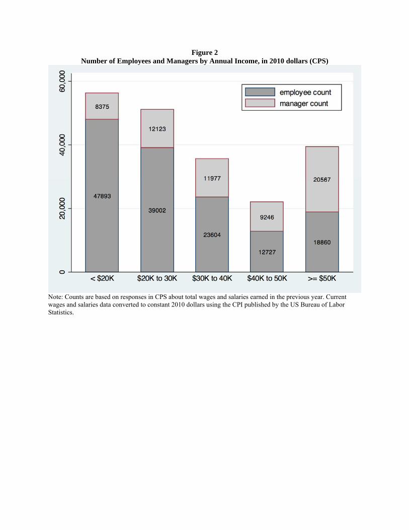
Figure 2 Number of Employees and Managers by Annual Income, in 2010 dollars (CPS)

Note: Counts are based on responses in CPS about total wages and salaries earned in the previous year. Current wages and salaries data converted to constant 2010 dollars using the CPI published by the US Bureau of Labor Statistics.

 

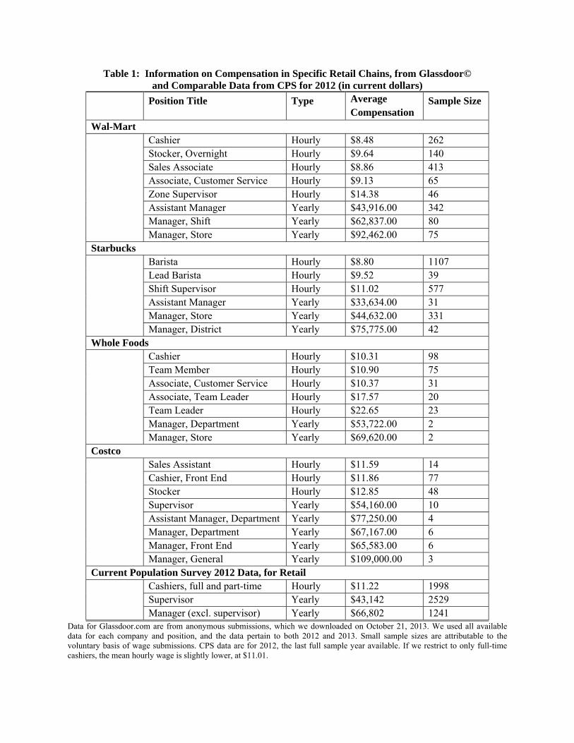
Table 1: Information on Compensation in Specific Retail Chains, from Glassdoor© and Comparable Data from CPS for 2012 (in current dollars)

Position Title Type Average Compensation

Sample Size

Wal-Mart

Cashier Hourly $8.48 262 Stocker, Overnight Hourly $9.64 140 Sales Associate Hourly $8.86 413 Associate, Customer Service Hourly $9.13 65 Zone Supervisor Hourly $14.38 46 Assistant Manager Yearly $43,916.00 342 Manager, Shift Yearly $62,837.00 80 Manager, Store Yearly $92,462.00 75

Starbucks Barista Hourly $8.80 1107 Lead Barista Hourly $9.52 39 Shift Supervisor Hourly $11.02 577 Assistant Manager Yearly $33,634.00 31 Manager, Store Yearly $44,632.00 331 Manager, District Yearly $75,775.00 42 Whole Foods Cashier Hourly $10.31 98 Team Member Hourly $10.90 75 Associate, Customer Service Hourly $10.37 31 Associate, Team Leader Hourly $17.57 20 Team Leader Hourly $22.65 23 Manager, Department Yearly $53,722.00 2 Manager, Store Yearly $69,620.00 2 Costco Sales Assistant Hourly $11.59 14 Cashier, Front End Hourly $11.86 77 Stocker Hourly $12.85 48 Supervisor Yearly $54,160.00 10 Assistant Manager, Department Yearly $77,250.00 4 Manager, Department Yearly $67,167.00 6 Manager, Front End Yearly $65,583.00 6 Manager, General Yearly $109,000.00 3 Current Population Survey 2012 Data, for Retail Cashiers, full and part-time Hourly $11.22 1998 Supervisor Yearly $43,142 2529 Manager (excl. supervisor) Yearly $66,802 1241

Data for Glassdoor.com are from anonymous submissions, which we downloaded on October 21, 2013. We used all available data for each company and position, and the data pertain to both 2012 and 2013. Small sample sizes are attributable to the voluntary basis of wage submissions. CPS data are for 2012, the last full sample year available. If we restrict to only full-time cashiers, the mean hourly wage is slightly lower, at $11.01.  

 

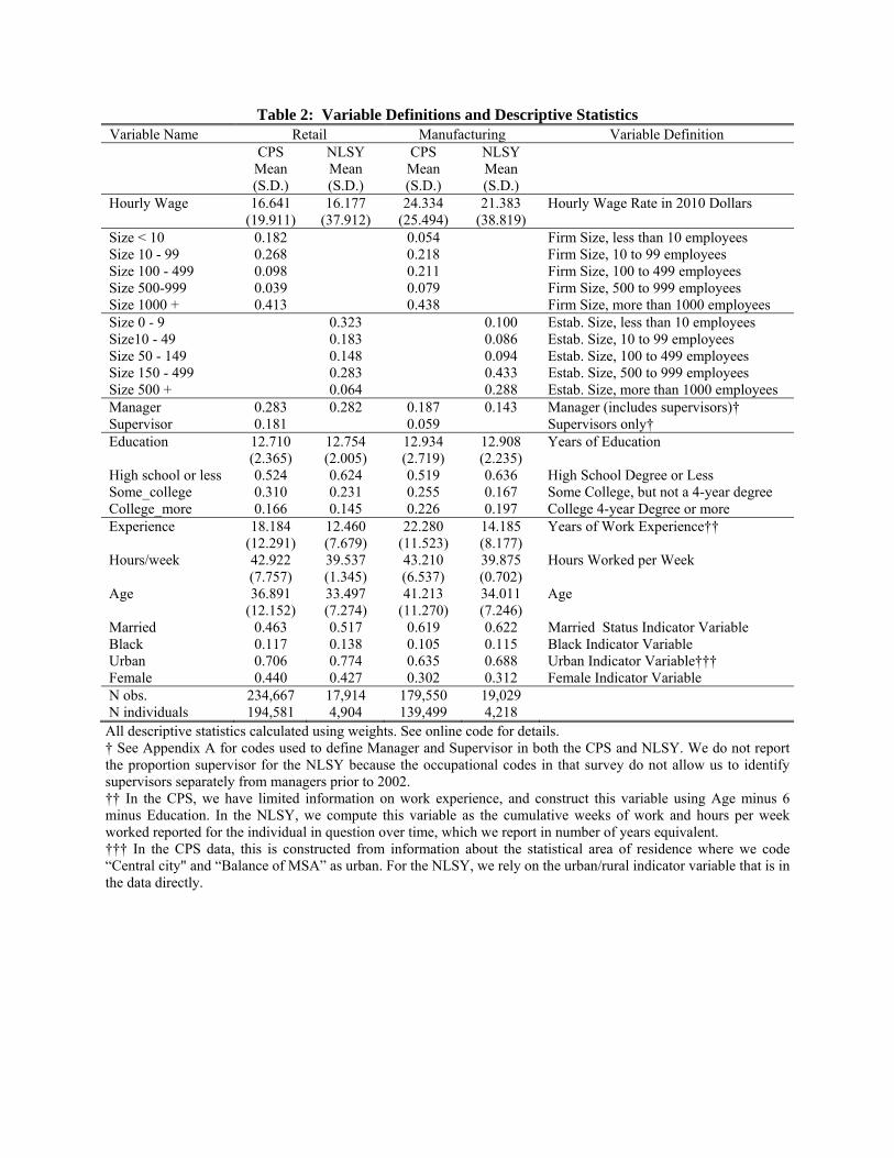
Table 2: Variable Definitions and Descriptive Statistics Variable Name Retail Manufacturing Variable Definition CPS

Mean (S.D.)

NLSY Mean (S.D.)

CPS Mean (S.D.)

NLSY Mean (S.D.)

Hourly Wage 16.641 16.177 24.334 21.383 Hourly Wage Rate in 2010 Dollars (19.911) (37.912) (25.494) (38.819) Size < 10 0.182 0.054 Firm Size, less than 10 employees Size 10 - 99 0.268 0.218 Firm Size, 10 to 99 employees Size 100 - 499 0.098 0.211 Firm Size, 100 to 499 employees Size 500-999 0.039 0.079 Firm Size, 500 to 999 employees Size 1000 + 0.413 0.438 Firm Size, more than 1000 employees Size 0 - 9 0.323 0.100 Estab. Size, less than 10 employees Size10 - 49 0.183 0.086 Estab. Size, 10 to 99 employees Size 50 - 149 0.148 0.094 Estab. Size, 100 to 499 employees Size 150 - 499 0.283 0.433 Estab. Size, 500 to 999 employees Size 500 + 0.064 0.288 Estab. Size, more than 1000 employees Manager 0.283 0.282 0.187 0.143 Manager (includes supervisors)† Supervisor 0.181 0.059 Supervisors only† Education 12.710 12.754 12.934 12.908 Years of Education (2.365) (2.005) (2.719) (2.235) High school or less 0.524 0.624 0.519 0.636 High School Degree or Less Some_college 0.310 0.231 0.255 0.167 Some College, but not a 4-year degree College_more 0.166 0.145 0.226 0.197 College 4-year Degree or more Experience 18.184 12.460 22.280 14.185 Years of Work Experience†† (12.291) (7.679) (11.523) (8.177) Hours/week 42.922 39.537 43.210 39.875 Hours Worked per Week (7.757) (1.345) (6.537) (0.702) Age 36.891 33.497 41.213 34.011 Age (12.152) (7.274) (11.270) (7.246) Married 0.463 0.517 0.619 0.622 Married Status Indicator Variable Black 0.117 0.138 0.105 0.115 Black Indicator Variable Urban 0.706 0.774 0.635 0.688 Urban Indicator Variable††† Female 0.440 0.427 0.302 0.312 Female Indicator Variable N obs. 234,667 17,914 179,550 19,029 N individuals 194,581 4,904 139,499 4,218

All descriptive statistics calculated using weights. See online code for details. † See Appendix A for codes used to define Manager and Supervisor in both the CPS and NLSY. We do not report the proportion supervisor for the NLSY because the occupational codes in that survey do not allow us to identify supervisors separately from managers prior to 2002. †† In the CPS, we have limited information on work experience, and construct this variable using Age minus 6 minus Education. In the NLSY, we compute this variable as the cumulative weeks of work and hours per week worked reported for the individual in question over time, which we report in number of years equivalent. ††† In the CPS data, this is constructed from information about the statistical area of residence where we code “Central city" and “Balance of MSA” as urban. For the NLSY, we rely on the urban/rural indicator variable that is in the data directly.

 

Table 3: Retail Trade by Education (CPS); Dependent Variable: Log Wage OLS OLS OLS OLS Fixed Effects Fixed Effects High School Some High School Some High School Some or Less College + or Less College + or Less College + Size 10-99 0.126*** 0.190*** 0.134*** 0.206*** 0.065*** 0.071*** (0.007) (0.009) (0.012) (0.015) (0.018) (0.025) Size 100-499 0.209*** 0.301*** 0.222*** 0.322*** 0.092*** 0.104*** (0.009) (0.010) (0.015) (0.018) (0.021) (0.028) Size 500-999 0.207*** 0.271*** 0.210*** 0.278*** 0.092*** 0.070** (0.011) (0.013) (0.019) (0.021) (0.025) (0.032) Size 1000+ 0.152*** 0.253*** 0.153*** 0.280*** 0.075*** 0.105*** (0.006) (0.008) (0.011) (0.014) (0.020) (0.026) Manager 0.226*** 0.195*** 0.209*** 0.158*** 0.083*** 0.065*** (0.005) (0.005) (0.008) (0.009) (0.015) (0.017) Education 0.052*** 0.093*** 0.053*** 0.086*** 0.020** 0.015 (0.001) (0.002) (0.002) (0.003) (0.008) (0.018) Experience 0.280*** 0.356*** 0.226*** 0.317*** 0.187** 0.371*** (0.006) (0.008) (0.013) (0.016) (0.079) (0.105) Experience2 -0.041*** -0.066*** -0.031*** -0.059*** -0.033** -0.061*** (0.001) (0.002) (0.003) (0.004) (0.016) (0.022) Female -0.252*** -0.211*** -0.266*** -0.197*** (0.004) (0.005) (0.008) (0.009) Married 0.115*** 0.153*** 0.116*** 0.157*** 0.038 0.023 (0.005) (0.005) (0.008) (0.010) (0.032) (0.039) Black -0.105*** -0.095*** -0.122*** -0.118*** (0.007) (0.008) (0.013) (0.017) Urban 0.087*** 0.144*** 0.087*** 0.147*** -0.529* 0.037 (0.005) (0.005) (0.008) (0.010) (0.317) (0.153) Constant 1.298*** 0.618*** 1.398*** 0.793*** 2.089*** 1.747*** (0.017) (0.028) (0.033) (0.054) (0.259) (0.313) Total Obs 125,115 109,552 39,856 35,276 39,856 35,276 Nb Individuals 105,187 91,409 19,928 17,638 19,928 17,638 Adjusted R2 0.162 0.219 0.165 0.194 0.445 0.516 Notes: All regressions include year fixed effects, and use CPS March Supplement weights. Clustered standard errors, at the individual level, in parentheses. * p<0.1; ** p<0.05; *** p<0.01. The educational categories are high school or less and some college or more. The first two columns show results for the larger sample available in the CPS. Columns 3 and 4 show results for the reduced sample corresponding to that used in the fixed effects regressions in Columns 5 and 6. Note that the sample sizes in columns 3 and 4, or in columns 5 and 6, do not sum to the number of matched individuals described in the text. This is because a number of the matched individuals switch education category between the two years we observe them.

 

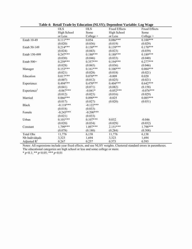
Table 4: Retail Trade by Education (NLSY); Dependent Variable: Log Wage OLS OLS Fixed Effects Fixed Effects High School Some High School Some or Less College + or Less College + Estab 10-49 0.111*** 0.054 0.086*** 0.100*** (0.020) (0.036) (0.019) (0.029) Estab 50-149 0.214*** 0.130*** 0.139*** 0.170*** (0.024) (0.043) (0.023) (0.039) Estab 150-499 0.247*** 0.180*** 0.188*** 0.189*** (0.030) (0.046) (0.033) (0.040) Estab 500+ 0.259*** 0.357*** 0.194*** 0.277*** (0.028) (0.065) (0.036) (0.046) Manager 0.153*** 0.161*** 0.100*** 0.084*** (0.021) (0.028) (0.018) (0.021) Education 0.017*** 0.070*** -0.009 0.020 (0.007) (0.012) (0.025) (0.021) Experience 0.494*** 0.470*** 0.404*** 0.642*** (0.041) (0.071) (0.082) (0.158) Experience2 -0.067*** -0.041* -0.052*** -0.076*** (0.012) (0.023) (0.016) (0.029) Married 0.066*** 0.090*** -0.025 0.085*** (0.017) (0.027) (0.020) (0.031) Black -0.118*** -0.122*** (0.018) (0.033) Female -0.243*** -0.200*** (0.021) (0.033) Urban 0.101*** 0.107*** 0.032 -0.046 (0.020) (0.034) (0.029) (0.032) Constant 1.799*** 1.097*** 2.151*** 1.798*** (0.078) (0.180) (0.284) (0.308) Total Obs 11,776 6,138 11,776 6,138 Nb Individuals 3,323 1,694 3,323 1,694 Adjusted R2 0.267 0.257 0.573 0.593 Notes: All regressions include year fixed effects, and use NLSY weights. Clustered standard errors in parentheses. The educational categories are high school or less and some college or more. * p<0.1; ** p<0.05; *** p<0.01

 

Table 5: Retail Trade by Gender (CPS); Dependent Variable: Log Wage OLS OLS OLS OLS Fixed Effects Fixed Effects female Male female male female male Size 10-99 0.163*** 0.146*** 0.168*** 0.160*** 0.034 0.083*** (0.008) (0.007) (0.015) (0.012) (0.021) (0.018) Size 100-499 0.259*** 0.243*** 0.266*** 0.265*** 0.088*** 0.104*** (0.010) (0.009) (0.017) (0.014) (0.026) (0.021) Size 500-999 0.254*** 0.224*** 0.230*** 0.249*** 0.051* 0.098*** (0.012) (0.011) (0.020) (0.019) (0.029) (0.026) Size 1000+ 0.225*** 0.178*** 0.236*** 0.194*** 0.083*** 0.082*** (0.008) (0.007) (0.013) (0.011) (0.023) (0.020) Manager 0.216*** 0.204*** 0.178*** 0.189*** 0.081*** 0.079*** (0.005) (0.005) (0.009) (0.008) (0.015) (0.016) Education 0.081*** 0.074*** 0.083*** 0.070*** 0.030*** 0.023*** (0.001) (0.001) (0.002) (0.002) (0.008) (0.008) Experience 0.254*** 0.341*** 0.183*** 0.294*** 0.262*** 0.148* (0.007) (0.007) (0.014) (0.013) (0.089) (0.079) Experience2 -0.040*** -0.054*** -0.028*** -0.046*** -0.040** -0.029* (0.002) (0.002) (0.003) (0.003) (0.017) (0.015) Married 0.066*** 0.191*** 0.060*** 0.195*** 0.020 0.056 (0.005) (0.005) (0.009) (0.008) (0.031) (0.035) Black -0.091*** -0.135*** -0.111*** -0.145*** (0.007) (0.008) (0.014) (0.015) Urban 0.154*** 0.097*** 0.159*** 0.092*** -0.471 -0.045 (0.005) (0.005) (0.009) (0.008) (0.439) (0.128) Constant 0.673*** 0.965*** 0.806*** 1.086*** 1.713*** 1.926*** (0.021) (0.017) (0.039) (0.033) (0.338) (0.174) Total Obs 105,976 128,691 34,644 45,528 34,644 45,528 Nb Individuals 88,654 105,927 17,322 22,764 17,322 22,764 Adjusted R2 0.169 0.225 0.173 0.210 0.468 0.506 Notes: All regressions include year fixed effects, and use CPS March Supplement weights. Clustered standard errors, at the individual level, in parentheses. * p<0.1; ** p<0.05; *** p<0.01. The first two columns show results for the larger sample available in the CPS. Columns 3 and 4 show results for the reduced sample corresponding to that used in the fixed effects regressions in Columns 5 and 6.

 

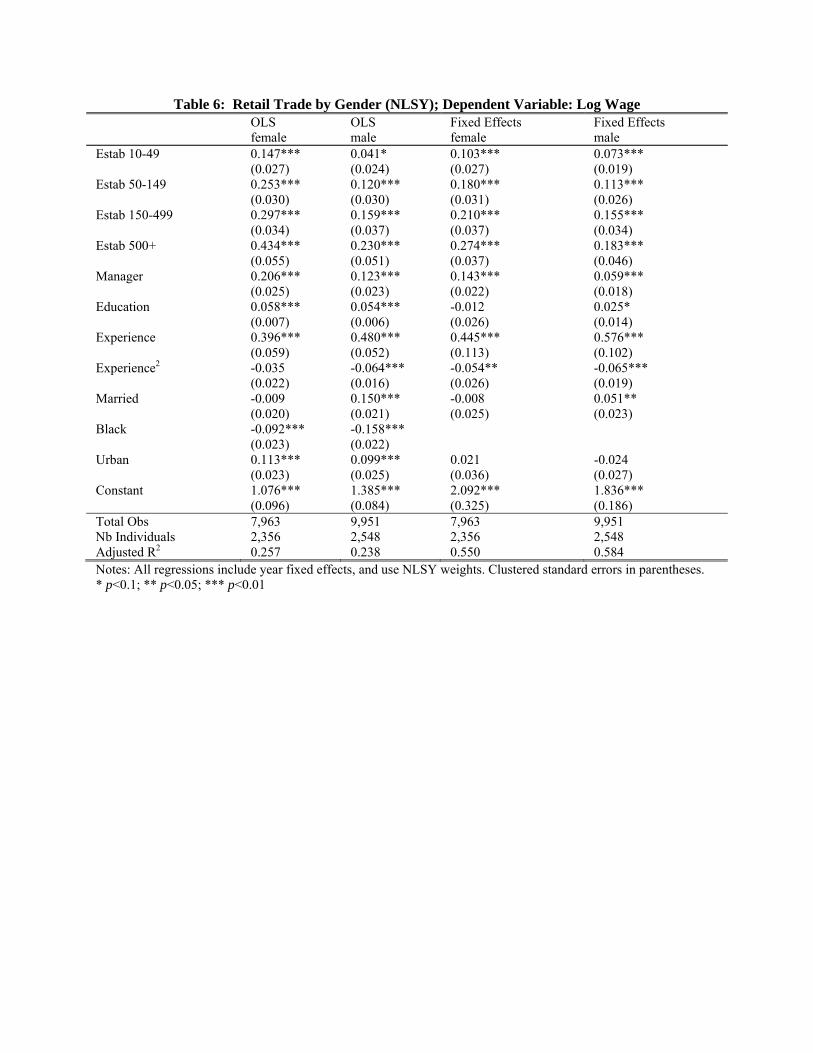
Table 6: Retail Trade by Gender (NLSY); Dependent Variable: Log Wage OLS OLS Fixed Effects Fixed Effects female male female male Estab 10-49 0.147*** 0.041* 0.103*** 0.073*** (0.027) (0.024) (0.027) (0.019) Estab 50-149 0.253*** 0.120*** 0.180*** 0.113*** (0.030) (0.030) (0.031) (0.026) Estab 150-499 0.297*** 0.159*** 0.210*** 0.155*** (0.034) (0.037) (0.037) (0.034) Estab 500+ 0.434*** 0.230*** 0.274*** 0.183*** (0.055) (0.051) (0.037) (0.046) Manager 0.206*** 0.123*** 0.143*** 0.059*** (0.025) (0.023) (0.022) (0.018) Education 0.058*** 0.054*** -0.012 0.025* (0.007) (0.006) (0.026) (0.014) Experience 0.396*** 0.480*** 0.445*** 0.576*** (0.059) (0.052) (0.113) (0.102) Experience2 -0.035 -0.064*** -0.054** -0.065*** (0.022) (0.016) (0.026) (0.019) Married -0.009 0.150*** -0.008 0.051** (0.020) (0.021) (0.025) (0.023) Black -0.092*** -0.158*** (0.023) (0.022) Urban 0.113*** 0.099*** 0.021 -0.024 (0.023) (0.025) (0.036) (0.027) Constant 1.076*** 1.385*** 2.092*** 1.836*** (0.096) (0.084) (0.325) (0.186) Total Obs 7,963 9,951 7,963 9,951 Nb Individuals 2,356 2,548 2,356 2,548 Adjusted R2 0.257 0.238 0.550 0.584 Notes: All regressions include year fixed effects, and use NLSY weights. Clustered standard errors in parentheses. * p<0.1; ** p<0.05; *** p<0.01

 

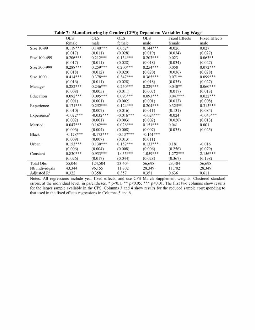
Table 7: Manufacturing by Gender (CPS); Dependent Variable: Log Wage OLS OLS OLS OLS Fixed Effects Fixed Effects female male female male female male Size 10-99 0.119*** 0.140*** 0.052* 0.144*** -0.026 0.027 (0.017) (0.011) (0.028) (0.019) (0.034) (0.027) Size 100-499 0.206*** 0.212*** 0.134*** 0.203*** 0.023 0.063** (0.017) (0.011) (0.028) (0.018) (0.034) (0.027) Size 500-999 0.288*** 0.259*** 0.200*** 0.254*** 0.058 0.072*** (0.018) (0.012) (0.029) (0.020) (0.036) (0.028) Size 1000+ 0.414*** 0.378*** 0.347*** 0.365*** 0.071** 0.099*** (0.016) (0.011) (0.028) (0.018) (0.035) (0.027) Manager 0.282*** 0.246*** 0.250*** 0.229*** 0.040** 0.060*** (0.008) (0.005) (0.011) (0.007) (0.017) (0.013) Education 0.092*** 0.095*** 0.093*** 0.093*** 0.047*** 0.022*** (0.001) (0.001) (0.002) (0.001) (0.013) (0.008) Experience 0.171*** 0.252*** 0.124*** 0.204*** 0.325** 0.313*** (0.010) (0.007) (0.016) (0.011) (0.131) (0.084) Experience2 -0.022*** -0.032*** -0.016*** -0.024*** -0.024 -0.043*** (0.002) (0.001) (0.003) (0.002) (0.020) (0.013) Married 0.047*** 0.162*** 0.026*** 0.151*** 0.041 0.001 (0.006) (0.004) (0.008) (0.007) (0.035) (0.025) Black -0.128*** -0.173*** -0.137*** -0.161*** (0.009) (0.007) (0.013) (0.011) Urban 0.153*** 0.130*** 0.152*** 0.133*** 0.181 -0.016 (0.006) (0.004) (0.008) (0.006) (0.256) (0.079) Constant 0.830*** 0.933*** 1.035*** 1.059*** 1.272*** 2.156*** (0.026) (0.017) (0.044) (0.028) (0.367) (0.198) Total Obs 55,046 124,504 23,404 56,698 23,404 56,698 Nb Individuals 43,344 96,155 11,702 28,349 11,702 28,349 Adjusted R2 0.322 0.358 0.357 0.351 0.636 0.611 Notes: All regressions include year fixed effects, and use CPS March Supplement weights. Clustered standard errors, at the individual level, in parentheses. * p<0.1; ** p<0.05; *** p<0.01. The first two columns show results for the larger sample available in the CPS. Columns 3 and 4 show results for the reduced sample corresponding to that used in the fixed effects regressions in Columns 5 and 6.

 

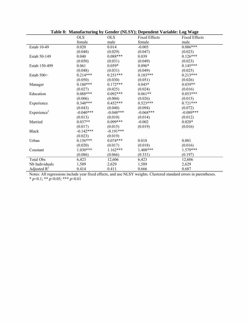
Table 8: Manufacturing by Gender (NLSY); Dependent Variable: Log Wage OLS OLS Fixed Effects Fixed Effects female male female male Estab 10-49 0.020 0.014 -0.005 0.086*** (0.048) (0.029) (0.047) (0.023) Estab 50-149 0.040 0.088*** 0.039 0.126*** (0.050) (0.031) (0.049) (0.023) Estab 150-499 0.061 0.059* 0.096* 0.145*** (0.048) (0.031) (0.049) (0.025) Estab 500+ 0.214*** 0.251*** 0.183*** 0.213*** (0.050) (0.030) (0.051) (0.026) Manager 0.180*** 0.172*** 0.045* 0.039** (0.027) (0.025) (0.024) (0.016) Education 0.088*** 0.092*** 0.061** 0.053*** (0.006) (0.004) (0.026) (0.015) Experience 0.348*** 0.452*** 0.523*** 0.721*** (0.043) (0.040) (0.094) (0.072) Experience2 -0.040*** -0.048*** -0.068*** -0.089*** (0.013) (0.010) (0.014) (0.012) Married 0.037** 0.099*** -0.002 0.028* (0.017) (0.015) (0.019) (0.016) Black -0.142*** -0.191*** (0.023) (0.019) Urban 0.156*** 0.074*** 0.018 0.001 (0.020) (0.017) (0.018) (0.016) Constant 1.030*** 1.162*** 1.408*** 1.579*** (0.086) (0.066) (0.331) (0.197) Total Obs 6,423 12,606 6,423 12,606 Nb Individuals 1,589 2,629 1,589 2,629 Adjusted R2 0.414 0.411 0.666 0.687 Notes: All regressions include year fixed effects, and use NLSY weights. Clustered standard errors in parentheses. * p<0.1; ** p<0.05; *** p<0.01

 

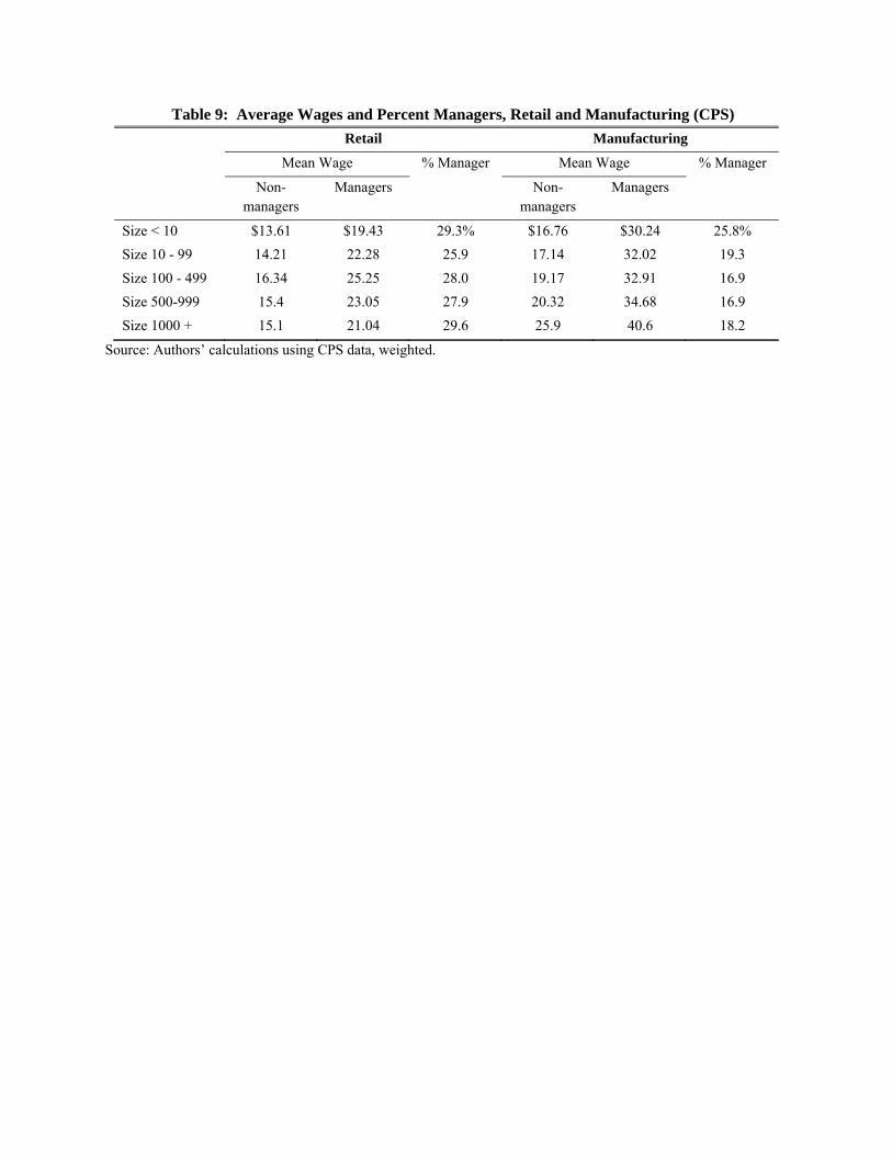
Table 9: Average Wages and Percent Managers, Retail and Manufacturing (CPS)

Retail Manufacturing

Mean Wage % Manager Mean Wage % Manager

Non-managers

Managers Non-managers

Managers

Size < 10 $13.61 $19.43 29.3% $16.76 $30.24 25.8%

Size 10 - 99 14.21 22.28 25.9 17.14 32.02 19.3

Size 100 - 499 16.34 25.25 28.0 19.17 32.91 16.9

Size 500-999 15.4 23.05 27.9 20.32 34.68 16.9

Size 1000 + 15.1 21.04 29.6 25.9 40.6 18.2

Source: Authors’ calculations using CPS data, weighted.

 

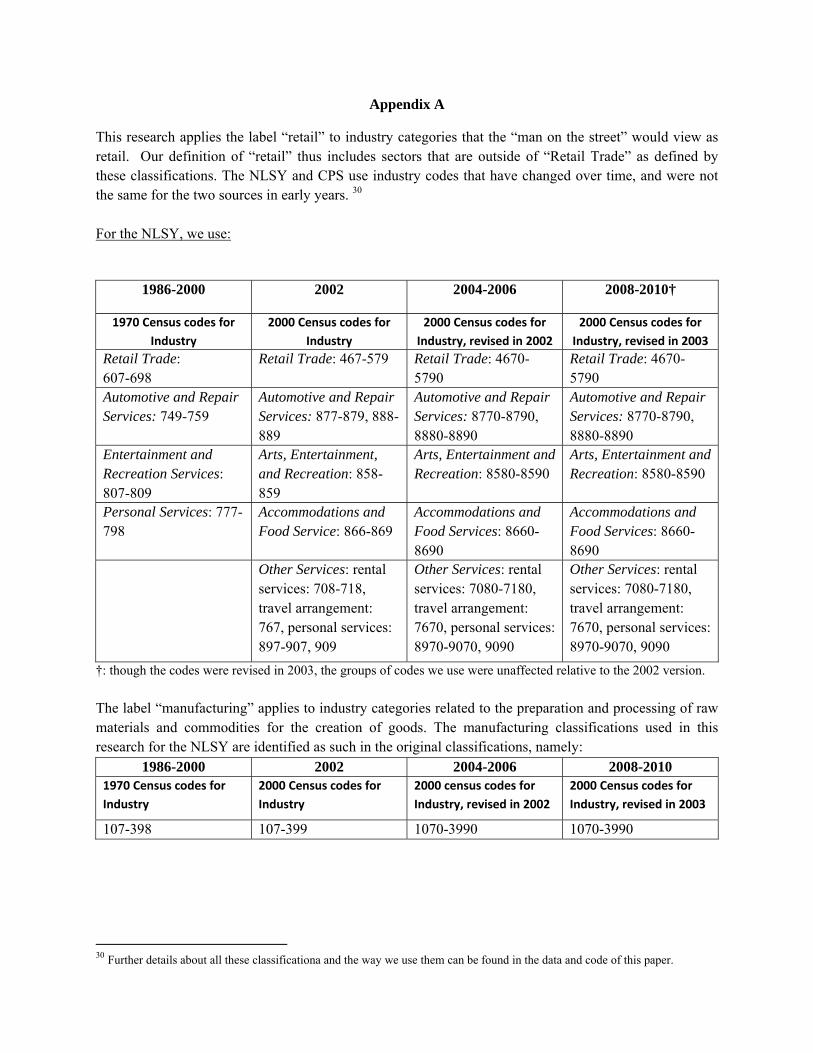
Appendix A

This research applies the label “retail” to industry categories that the “man on the street” would view as retail. Our definition of “retail” thus includes sectors that are outside of “Retail Trade” as defined by these classifications. The NLSY and CPS use industry codes that have changed over time, and were not the same for the two sources in early years. 30 For the NLSY, we use:

 

1986-2000 2002 2004-2006 2008-2010†

1970 Census codes for 

Industry 2000 Census codes for 

Industry 2000 Census codes for 

Industry, revised in 2002 2000 Census codes for 

Industry, revised in 2003 Retail Trade: 607-698

Retail Trade: 467-579 Retail Trade: 4670-5790

Retail Trade: 4670-5790

Automotive and Repair Services: 749-759

Automotive and Repair Services: 877-879, 888-889

Automotive and Repair Services: 8770-8790, 8880-8890

Automotive and Repair Services: 8770-8790, 8880-8890

Entertainment and Recreation Services: 807-809

Arts, Entertainment, and Recreation: 858-859

Arts, Entertainment and Recreation: 8580-8590

Arts, Entertainment and Recreation: 8580-8590

Personal Services: 777-798

Accommodations and Food Service: 866-869

Accommodations and Food Services: 8660-8690

Accommodations and Food Services: 8660-8690

Other Services: rental services: 708-718, travel arrangement: 767, personal services: 897-907, 909

Other Services: rental services: 7080-7180, travel arrangement: 7670, personal services: 8970-9070, 9090

Other Services: rental services: 7080-7180, travel arrangement: 7670, personal services: 8970-9070, 9090

†: though the codes were revised in 2003, the groups of codes we use were unaffected relative to the 2002 version.

The label “manufacturing” applies to industry categories related to the preparation and processing of raw materials and commodities for the creation of goods. The manufacturing classifications used in this research for the NLSY are identified as such in the original classifications, namely:

1986-2000 2002 2004-2006 2008-2010 1970 Census codes for 

Industry 2000 Census codes for 

Industry 2000 census codes for 

Industry, revised in 2002 2000 Census codes for 

Industry, revised in 2003

107-398 107-399 1070-3990 1070-3990

                                                            30 Further details about all these classificationa and the way we use them can be found in the data and code of this paper.

 

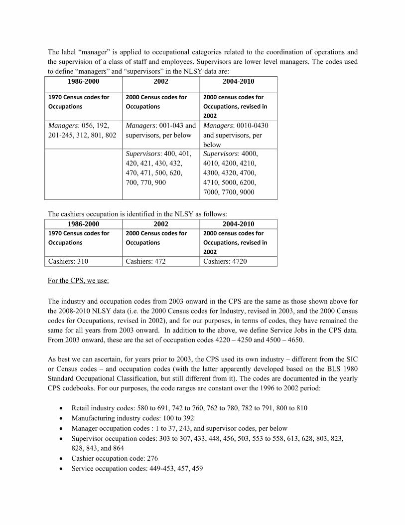
The label “manager” is applied to occupational categories related to the coordination of operations and the supervision of a class of staff and employees. Supervisors are lower level managers. The codes used to define “managers” and “supervisors” in the NLSY data are:

1986-2000 2002 2004-2010

1970 Census codes for 

Occupations 2000 Census codes for 

Occupations 2000 census codes for 

Occupations, revised in 

2002 Managers: 056, 192, 201-245, 312, 801, 802

Managers: 001-043 and supervisors, per below

Managers: 0010-0430 and supervisors, per below

Supervisors: 400, 401, 420, 421, 430, 432, 470, 471, 500, 620, 700, 770, 900

Supervisors: 4000, 4010, 4200, 4210, 4300, 4320, 4700, 4710, 5000, 6200, 7000, 7700, 9000

The cashiers occupation is identified in the NLSY as follows:

1986-2000 2002 2004-2010 1970 Census codes for 

Occupations 2000 Census codes for 

Occupations 2000 census codes for 

Occupations, revised in 

2002 Cashiers: 310 Cashiers: 472 Cashiers: 4720 For the CPS, we use:

 

The industry and occupation codes from 2003 onward in the CPS are the same as those shown above for the 2008-2010 NLSY data (i.e. the 2000 Census codes for Industry, revised in 2003, and the 2000 Census codes for Occupations, revised in 2002), and for our purposes, in terms of codes, they have remained the same for all years from 2003 onward. In addition to the above, we define Service Jobs in the CPS data. From 2003 onward, these are the set of occupation codes 4220 – 4250 and 4500 – 4650. As best we can ascertain, for years prior to 2003, the CPS used its own industry – different from the SIC or Census codes – and occupation codes (with the latter apparently developed based on the BLS 1980 Standard Occupational Classification, but still different from it). The codes are documented in the yearly CPS codebooks. For our purposes, the code ranges are constant over the 1996 to 2002 period:

  Retail industry codes: 580 to 691, 742 to 760, 762 to 780, 782 to 791, 800 to 810

Manufacturing industry codes: 100 to 392

Manager occupation codes : 1 to 37, 243, and supervisor codes, per below

Supervisor occupation codes: 303 to 307, 433, 448, 456, 503, 553 to 558, 613, 628, 803, 823, 828, 843, and 864

Cashier occupation code: 276

Service occupation codes: 449-453, 457, 459

 

Table A1: Descriptive Statistics For the Combination of Full and Part-Time Workers Variable Name Retail Manufacturing CPS

Mean (S.D.)

NLSY Mean (S.D.)

CPS Mean (S.D.)

NLSY Mean (S.D.)

Hourly Wage 15.730 15.610 24.378 21.352 (23.996) (37.396) (31.169) (38.509) Size < 10 0.184 0.062 Size 10 - 99 0.265 0.222 Size 100 - 499 0.089 0.209 Size 500-999 0.038 0.077 Size 1000 + 0.424 0.429 Size 0 - 9 0.335 0.111 Size10 - 49 0.190 0.089 Size 50 - 149 0.146 0.094 Size 150 - 499 0.276 0.424 Size 500 + 0.054 0.281 Manager 0.216 0.226 0.183 0.141 Supervisor 0.139 0.057 Education 12.657 12.739 12.917 12.918 (2.235) (2.003) (2.716) (2.245) High school or less 0.516 0.626 0.519 0.632 Some_college 0.339 0.235 0.257 0.170 College_more 0.144 0.139 0.224 0.199 Experience 16.160 11.389 22.103 13.990 (12.921) (7.512) (11.680) (8.186) Hours/week 36.590 35.196 42.238 39.091 (12.234) (8.616) (7.897) (4.222) Age 34.807 33.371 41.018 33.962 (12.855) (7.267) (11.442) (7.231) Married 0.411 0.531 0.612 0.623 Black 0.116 0.132 0.104 0.114 Urban 0.698 0.776 0.635 0.687 Female 0.503 0.514 0.315 0.327 N obs. 337,389 23,764 188,766 19,859 N individuals 276,061 5,903 146,895 4,426

All descriptive statistics calculated using weights. See online code for details. † See Appendix A for codes used to define Manager and Supervisor in both the CPS and NLSY. We do not report the proportion supervisor for the NLSY because the occupational codes in that survey do not allow us to identify supervisors separately from managers prior to 2002. †† In the CPS, we have limited information on work experience, and construct this variable using Age minus 6 minus Education. In the NLSY, we compute this variable as the cumulative weeks of work and hours per week worked reported for the individual in question over time, which we report in number of years equivalent. ††† In the CPS data, this is constructed from information about the statistical area of residence where we code “Central city" and “Balance of MSA” as urban. For the NLSY, we rely on the urban/rural indicator variable that is in the data directly.