Do Futures and Options trading increase stock market volatility?

Dr. Premalata Shenbagaraman∗

Abstract

The objective of this study is to assess the impact of introducing index futures and options

contracts on the volatility of the underlying stock index in India. Numerous studies on the

effects of futures and options listing on the underlying cash market volatility have been

done in the developed markets. The empirical evidence is mixed and most suggest that the

introduction of derivatives do not destabilize the underlying market. The studies also show

that the introduction of derivative contracts improves liquidity and reduces informational

asymmetries in the market. In the late nineties, many emerging and transition economies

have introduced derivative contracts, raising interesting issues unique to these markets.

Emerging stock markets operate in very different economic, political, technological and

social environments than markets in developed countries like the USA or the UK. This

paper explores the impact of the introduction of derivative trading on cash market

volatility using data on stock index futures and options contracts traded on the S & P CNX

Nifty (India). The results suggest that futures and options trading have not led to a change

in the volatility of the underlying stock index, but the nature of volatility seems to have

changed post-futures. We also examine whether greater futures trading activity (volume

and open interest) is associated with greater spot market volatility. We find no evidence of

any link between trading activity variables in the futures market and spot market volatility.

The results of this study are especially important to stock exchange officials and regulators

in designing trading mechanisms and contract specifications for derivative contracts,

thereby enhancing their value as risk management tools

∗ CFA, Department of Finance, Clemson University, Clemson, USA. The views expressed and the approach suggested are of the authors and not necessarily of NSE.

2

I. Introduction

In the last decade, many emerging and transition economies have started introducing derivative

contracts. As was the case when commodity futures were first introduced on the Chicago Board of

Trade in 1865, policymakers and regulators in these markets are concerned about the impact of

futures on the underlying cash market. One of the reasons for this concern is the belief that futures

trading attracts speculators who then destabilize spot prices. This concern is evident in the following

excerpt from an article by John Stuart Mill (1871):

“The safety and cheapness of communications, which enable a deficiency in one

place to be, supplied from the surplus of another render the fluctuations of prices

much less extreme than formerly. This effect is much promoted by the existence of

speculative merchant. Speculators, therefore, have a highly useful office in the

economy of society”.

Since futures encourage speculation, the debate on the impact of speculators intensified

when futures contracts were first introduced for trading; beginning with commodity futures and

moving on to financial futures and recently futures on weather and electricity. However, this

traditional favorable view towards the economic benefits of speculative activity has not always been

acceptable to regulators. For example, futures trading was blamed by some for the stock market

crash of 1987 in the USA, thereby warranting more regulation. However before further regulation in

introduced, it is essential to determine whether in fact there is a causal link between the introduction

of futures and spot market volatility. It therefore becomes imperative that we seek answers to

questions like: What is the impact of derivatives upon market efficiency and liquidity of the

underlying cash market? To what extent do derivatives destabilize the financial system, and how

should these risks be addressed? Can the results from studies of developed markets be extended to

emerging markets?

This paper seeks to contribute to the existing literature in many ways. This is the first study

to examine the impact of financial derivatives introduction on cash market volatility in an emerging

market, India. Further, this study improves upon the methodology used in prior studies by using a

framework that allows for generalized auto-regressive conditional heteroskedasticity (GARCH) i.e., it

explicitly models the volatility process over time, rather than using estimated standard deviations to

measure volatility. This estimation technique enables us to explore the link between

information/news arrival in the market and its effect on cash market volatility. The study also looks

at the linkages in ongoing trading activity in the futures market with the underlying spot market

volatility by decomposing trading volume and open interest into an expected component and an

unexpected (surprise) component. Finally this is the first study to our knowledge that looks at the

3

effects of both stock index futures introduction as well as stock index options introduction on the

underlying cash market volatility.

The results of this study are crucial to investors, stock exchange officials and regulators.

Derivatives play a very important role in the price discovery process and in completing the market.

Their role in risk management for institutional investors and mutual fund managers need hardly be

overemphasized. This role as a tool for risk management clearly assumes that derivatives trading do

not increase market volatility and risk. The results of this study will throw some light on the effects

of derivative introduction on the efficiency and volatility of the underlying cash markets.

The study is organized as follows. Section II discusses the theoretical debate and summarizes

the empirical literature on derivative listing effects, Section III details the model and the econometric

methodology used in this study, Section IV outlines the data used and discusses the main results of

the model and finally Section V concludes the study and presents directions for future research.

II. Theoretical foundations and survey of the empirical literature.

The introduction of equity index futures markets enables traders to transact large volumes at much

lower transaction costs relative to the cash market. The consequence of this increase in order flow to

futures markets is unresolved on both a theoretical and an empirical front. Stein (1987) develops a

model in which prices are determined by the interaction between hedgers and informed speculators.

In this model, opening a futures market has two effects; (1). The futures market improves risk

sharing and therefore reduces price volatility, and (2). If the speculators observe a noisy but

informative signal, the hedgers react to the noise in the speculative trades, producing an increase in

volatility.

In contrast, models developed by Danthine (1978) argue that the futures markets improve

market depth and reduce volatility because the cost to informed traders of responding to mispricing

is reduced. Froot and Perold(1991) extend Kyle’s(1985) model to show that market depth is

increased by more rapid dissemination of market-wide information and the presence of market

makers in the futures market in addition to the cash market. Ross (1989) assumes that there exists an

economy that is devoid of arbitrage and proceeds to provide a condition under which the no-

arbitrage situation will be sustained. It implies that the variance of the price change will be equal to

the rate of information flow. The implication of this is that the volatility of the asset price will

increase as the rate of information flow increases. Thus, if futures increase the flow of information,

than in the absence of arbitrage opportunity, the volatility of the spot price must change. Overall, the

theoretical work on futures listing effects offer no consensus on the size and the direction of the

change in volatility. We therefore need to turn to the empirical literature on evidence relating to the

volatility effects of listing index futures and options.

4

The first stock index futures contract introduced in the world was the Value line contract,

introduced by the Kansas City Board of Trade in 1982 in the USA. Since then we have seem

numerous markets all over the world launching new derivative contracts every year. Following the

introduction of derivative contracts in developed markets like the US and UK, researchers have

sought to analyze the impact of derivatives introduction on the volatility and efficiency of the

underlying cash market. The empirical evidence is however quite mixed. Most studies summarize that

the introduction of derivatives does not destabilize the underlying market; either there is no effect or

perhaps only a very small decline in volatility1. The impact however, seems to vary depending on the

time period studied and the country studied. For example, in a study of 25 countries, Gulen and

Mayhew (2000) find that futures trading is associated with increased volatility in the United States

and Japan. In some countries, there is no robust, significant effect, and in many others, volatility is

lower after futures have been introduced.

Nathan Associates (1974) was the first to study the impact of listing options on the Chicago

Board of Exchange. He reported that the introduction of options seemed to have helped stabilize

trading in the underlying stocks. This result has been supported by Skinner (1989) and also by other

authors for the UK, Canada, Switzerland and Sweden. More recent work by Lamoureux and

Pannikath (1994), Freund, McCann and Webb (1994) and Bollen (1998) have found that the

direction of the volatility effect is not consistent over time. After 1987, the residual variance of both

optioned stocks and stocks in a matched control group increased at the time of the option listing.

This might be interpreted in two ways; viz. perhaps the listing has no true impact on volatility and

there is some common unknown factor that is driving the magnitude of the idiosyncratic risk for

different stocks. Or perhaps, there are spill over effects associated with listing options for some

stocks, such that the dynamics of other stocks also changes (Detemple and Jorion, 1990, and Cao

1999).

In looking at the effect on liquidity, Nathan Associates (1974) found that the trading volume

did not change with option introduction. However, later studies like Kumar, Sarin and Shastri (1995)

have found that the volume in the underlying stock does increase after the introduction of stock

options. Studies have also found that after the introduction of options, prices tend to reflect new

information more quickly, bid-ask spreads narrow, and the adverse selection component of the

spread becomes smaller. Relatively few authors have studied the impact of stock index options listing

on volatility in the cash market. Evidence reported by Chatrath, Kamath, Chakornpipat and

Ramchander (1995) indicates that S&P 100 stock index options trading had a stabilizing effect on the

1 For a detailed summary of this literature, see surveys by Hodges (1992), Damodaran and Subrahmanyam (1992), Stucliffe (1997) and Mayhew (1999).

5

underlying stock index. Studies of volatility effects of individual equity options have also reported

mixed results; some find that volatility is unchanged, while some report a small decrease in volatility.

Only one paper Wei, Poon and Zee (1997) report an increase in volatility for options on OTC stocks

in the USA. However no consensus result emerges, which probably a result of different data and

time-periods studied, as also the inherent endogenously of the option listing decision2.

III. Model and Methodology

One of the key assumptions of the ordinary regression model is that the errors have the same

variance throughout the sample. This is also called the homoscedasticity model. If the error variance

is not constant, the data are said to be heteroscedastic. Since ordinary least-squares regression

assumes constant error variance, heteroscedasticity causes the OLS estimates to be inefficient.

Models that take into account the changing variance can make more efficient use of the data. There

are several approaches to dealing with heteroscedasticity. If the error variance at different times is

known, weighted regression is a good method. If, as is usually the case, the error variance is unknown

and must be estimated from the data, one can model the changing error variance. In the past, studies

of volatility have used constructed volatility measures like estimated standard deviations, rolling

standard deviations, etc, to discern the effect of futures introduction. These studies implicitly assume

that price changes in spot markets are serially uncorrelated and homoscedastic. However, findings of

heteroskedasticity in stock returns are well documented (Mandelbrot 1963), Fama (1965), Bollerslev

(1986). Thus the observed differences in variances from models assuming homoscedasticity may

simply be due to the effect of return dependence and not necessarily due to futures introduction. The

GARCH model assumes conditional heteroscedasticity, with homoscedastic unconditional error

variance. That is, the model assumes that the changes in variance are a function of the realizations of

preceding errors and that these changes represent temporary and random departures from a constant

unconditional variance, as might be the case when using daily data. The advantage of a GARCH

model is that it captures the tendency in financial data for volatility clustering. It therefore enables us

to make the connection between information and volatility explicit, since any change in the rate of

information arrival to the market will change the volatility in the market. Thus, unless information

remains constant, which is hardly the case, volatility must be time varying, even on a daily basis. A

model with errors that follow a GARCH (p,q) process is represented as follows:

2 In a recent working paper, Mayhew and Mihow (2000) explicitly model the exchanges’ option listing choice using a logit model to account for this endogeniety.

6

∑∑=

−=

−

−

++=

Ψ++=q

jjtj

p

itit

ttttt

hh

hNXaaY

11

210

110 ),0(~,

βεαα

εε Equation 1a and 1b

where Equation 1a is the conditional mean equation and 1b is the conditional variance equation.

In studying the links between information, cash market volatility and derivatives trading, two issues

are interesting. First, how the initial introduction of derivative contracts impact cash market volatility.

Second, whether the existence of futures trading affects daily volatility in the cash market. To address

the first issue, we introduce a dummy variable into the conditional variance equation. Equation (1)

thus becomes:

DFhh

hNXaaYq

jjtj

p

itit

ttttt

γβεαα

εε

+++=

Ψ++=

∑∑=

−=

−

−

11

210

110 ),0(~, Equation 2

where DF is a dummy variable taking the value of 0 before futures introduction and 1 after. If the

coefficient on the Dummy is statistically significant then the introduction of futures has an impact on

the spot market volatility. To address the second issue, we divide the sample into the pre-futures and

post- futures sub-sample and a GARCH model is estimated separately for each sub-sample. This

allows us to compare the nature of volatility before and after the onset of futures trading. Further, we

also incorporate the contract volume and open interest in the futures market in the conditional

variance equation in the post-futures sub sample.

The impact of stock index futures and option contract introduction in the Indian market is

examined using a univariate GARCH (1,1) model3. The time series of daily returns on the S&P CNX

Nifty Index is modeled as a univariate GARCH process. Following Pagan and Schwert (1990) and

Engle and Ng (1993), we need to remove from the time series any predictability associated with

lagged world returns and/or day of the week effects. Further, we need to control for the effect of

market wide factors, since we are interested in isolating the unique impact of the introduction of the

futures/options contracts. Fortunately for the Indian stock market we have another index, the Nifty

Junior, which comprises stocks for which no futures contracts are traded. As such, it serves as a

perfect control variable for us to isolate market wide factors and thereby concentrate on the residual

volatility in the Nifty as a direct result of the introduction of the index derivative contracts. We

therefore introduce the return on the Nifty Junior index as an additional independent variable. The

following conditional mean equation is estimated:

3 Alternative GARCH models were estimated, the GJR-GARCH, EGARCH AND TGARCH, but we find the GARCH (1,1) model to provide the best fit for the data in this study.

7

tj

jjtrniftyjuniotsptnifty uDAYRRR ++++= ∑=

−

5

2,21,50010, αααα Equation 3

where tniftyR , is the daily return on the S&P CNX Nifty Index calculated as the first difference of the

log of the index, 1,500 −tspR is the lagged S&P500 index return, and DAYj are day-of-the-week dummy

variables for Tuesday to Friday. The lagged S&P500 index return is used as an independent variable

to remove the effects of worldwide price movements on the volatility of the Nifty Index return. For

example, if the Indian market is influenced by US markets, this will be reflected through the lagged

S&P500 return.

In GARCH, the residuals { }tu from Equation 3 are assumed to be distributed ( )thN ,0 where the

conditional volatility th is given by the following equation:

tttt Dhh 3122

110 γγεγγ +++= −− Equation 4

where tD is a dummy variable that takes on a value of zero before the options/futures were

introduced and a value of one after. A significant positive value for 3γwould indicate that derivatives

introduction increases the volatility of the underlying index.

Section IV. Data and Results

Daily closing prices for the period 5th Oct 1995 to 31st Dec 2002 for the SNX Nifty and the Nifty

Junior were obtained from the CD-ROMs provided by NSE and the NSE website. Data on Nifty

futures contract volume and open interest were downloaded from the NSE website. Data on the

S&P500 index were obtained from Reuters Inc. All estimations in this study are done using SAS.

The SNX Nifty is an index of 50 stocks traded on the National Stock Exchange and represents

approximately 50% of the total market capitalization of the market. Nifty Junior is an index of the

next most liquid 50 stocks. The first index future in India was introduced on the SNX Nifty on June

12, 2000. The first index options contract was introduced on 4th June, 2001.

Table 1 provides summary statistics for the Nifty and Nifty Junior indices. All returns are

calculated as the first difference of the log of the index daily close price and Chart 1 graphs the

returns on the Nifty index over time. As seen in Table 1, the overall sample has 1805 time series

observations. The mean return on the Nifty is 0.003% per day with a standard deviation of 1.67%

per day. The mean daily return on the Nifty Junior is 0.007% with a standard deviation of 1.95%. If

we divide the sample period into pre-futures vs. post-futures using the June 12, 2000 cutoff date, the

mean daily return on the Nifty is a positive 0.029% before and a negative 0.044% after the futures

8

was introduced. A similar pattern in Nifty Junior returns is also apparent. The average daily standard

deviation for the Nifty return pre-futures is 1.79% and 1.42% post-futures. However, the daily

standard deviation for the Nifty Junior, for which no index futures were traded, pre-futures is 2%

and post futures is 1.7%. A very similar pattern emerges when one examines the pre-options and

post-option sub-sample means and standard deviations.

As stated in the previous section, it is important to remove market-wide influences on Nifty

returns, if we are to isolate the impact of futures introduction. In order to do this we need a proxy

that is not associated with any futures contract, and yet captures market-wide influences in India. For

example, information news releases relating to economic conditions like, inflation rates, growth

forecasts, exchange rates, etc are likely to affect the whole market. It is necessary to remove the

effects for all these factors on price volatility. Since the Nifty Junior has no futures contracts traded

on it, we use it as a proxy to capture market-wide information effects. Following Pagan and Schwert

(1990) and Engle and Ng (1993), we also need to remove from the time series any predictability

associated with lagged world market returns and day-of-the-week effects. The lagged return on the

S&P500 index is used as a proxy for the world market return to remove any worldwide price

movements on volatility in the Nifty return. We introduce day of the week dummies for Tuesday to

Friday. Table 3 examines the Nifty returns for the presence of any ARCH/GARCH effects and finds

that there exists substantial ARCH effects in the residuals and therefore a model that accounts for

these effects would describe the data better.

Having demonstrated the need to use some type of GARCH model to model the Nifty

returns, we conducted tests to see which form of the GARCH model fits the returns data best. We

tested the GARCH (1,1) model, the EGARCH model of Nelson (1991), the GARCH model with t-

distribution and the GJR-GARCH model of Glosten, Jagannathan and Runkle (1993). We find that

the GARCH (1,1) and the EGARCH model both seem to fit the data better than the GJR-GARCH

and the TGARCH models. However, forecasting the multi-period error variance is easier in the

GARCH (1,1) model relative to the EGARCH model, and hence in the interest of practicality, we

use the GARCH (1,1) model in this study.

As mentioned earlier, in order to estimate the impact of the introduction of the futures and

options contracts, we introduce a Dummy variable in the conditional volatility equation. A significant

positive co-efficient would indicate and increase in volatility, a significant negative coefficient would

indicate a decrease in volatility. The results of the estimation for the impact of futures introduction

are presented in Table 4. The coefficient on the futures dummy 3γ, is not significantly different from

zero, indicating no impact on volatility. There appears to be significant day-of-the-week effects as

evidenced by the coefficients on the dummies for Tuesday and Friday. 1γ can be viewed as a “news”

9

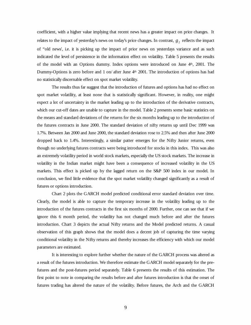
coefficient, with a higher value implying that recent news has a greater impact on price changes. It

relates to the impact of yesterday’s news on today’s price changes. In contrast, 2γ reflects the impact

of “old news', i.e. it is picking up the impact of prior news on yesterdays variance and as such

indicated the level of persistence in the information effect on volatility. Table 5 presents the results

of the model with an Options dummy. Index options were introduced on June 4th, 2001. The

Dummy-Options is zero before and 1 on/after June 4th 2001. The introduction of options has had

no statistically discernable effect on spot market volatility.

The results thus far suggest that the introduction of futures and options has had no effect on

spot market volatility, at least none that is statistically significant. However, in reality, one might

expect a lot of uncertainty in the market leading up to the introduction of the derivative contracts,

which our cut-off dates are unable to capture in the model. Table 2 presents some basic statistics on

the means and standard deviations of the returns for the six months leading up to the introduction of

the futures contracts in June 2000. The standard deviation of nifty returns up until Dec 1999 was

1.7%. Between Jan 2000 and June 2000, the standard deviation rose to 2.5% and then after June 2000

dropped back to 1.4%. Interestingly, a similar patter emerges for the Nifty Junior returns, even

though no underlying futures contracts were being introduced for stocks in this index. This was also

an extremely volatility period in world stock markets, especially the US stock markets. The increase in

volatility in the Indian market might have been a consequence of increased volatility in the US

markets. This effect is picked up by the lagged return on the S&P 500 index in our model. In

conclusion, we find little evidence that the spot market volatility changed significantly as a result of

futures or options introduction.

Chart 2 plots the GARCH model predicted conditional error standard deviation over time.

Clearly, the model is able to capture the temporary increase in the volatility leading up to the

introduction of the futures contracts in the first six months of 2000. Further, one can see that if we

ignore this 6 month period, the volatility has not changed much before and after the futures

introduction. Chart 3 depicts the actual Nifty returns and the Model predicted returns. A casual

observation of this graph shows that the model does a decent job of capturing the time varying

conditional volatility in the Nifty returns and thereby increases the efficiency with which our model

parameters are estimated.

It is interesting to explore further whether the nature of the GARCH process was altered as

a result of the futures introduction. We therefore estimate the GARCH model separately for the pre-

futures and the post-futures period separately. Table 6 presents the results of this estimation. The

first point to note in comparing the results before and after futures introduction is that the onset of

futures trading has altered the nature of the volatility. Before futures, the Arch and the GARCH

10

effects are significant, suggesting that both recent news and old news had a lingering impact on spot

volatility. The results also show the presence of day-of-the-week effects for Tuesday and Friday.

After the futures introduction, the day-of-the-weeks effects are no longer statistically significant. Also

the coefficient on the GARCH variable is no longer significant, suggesting that old news has no

impact on today’s spot price changes. However our sample period post futures is fairly small, only

597 observations, so we must treat these results with some caution. The results are similar when we

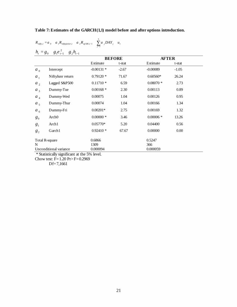
analyze the GARCH effects pre and post options introduction in Table 7.

We have thus far, tested whether there appears to be any structural change in the underlying

spot market volatility at the time of futures and options introduction. It is interesting to see if there

has been any structural change in the mean equation pre and post futures/options introduction. In

order to test for parameter stability in the mean equation, assuming constant unconditional variance,

we conduct a Chow test for structural change. The Chow test is a formal test to evaluate the stability

of the regression coefficients. The sample is divided into two parts at the specified break-point, and

the fit of the model in the two parts is compared to test whether both sub samples are consistent

with the same model. The Null Hypothesis is that the coefficients in both sub-samples are equal,

conditional on the same error variance. Under the Null, the Chow test statistic has an F-distribution

with K and (n1+n2-2k) degrees of freedom where k is the number of coefficients. Using June 12,

2000 as our first break point for futures introduction, the value of the F-stat (7, 1661) df is 3.63 and

is highly significant at the 1% level. This suggests that the coefficients are not the same before and

after futures introduction. Using June 3, 2001 as our breakpoint for options introduction, the F-stat

(7, 1661) df is 1.20 and we are unable to reject the null that the coefficients are the same.

Now we test to see if there is any relationship, after the futures are introduced, between the

level of futures trading activity and the volatility of the spot market return. We follow Bessembinder

and Sequin (1992) and using an ARIMA (p,q) model, decompose the time series of the futures

trading volume and open interest into expected and unexpected components. The expected

component represents a threshold level (or average) of futures trading, and the unexpected

component picks up any sudden increase in trading volume as a result of unexpected price changes.

Bessembinder and Sequin find that spot market volatility in the US market is positively related to the

unexpected components of volume and open interest, and negatively related to the expected

component, suggesting an increase in volatility due to unexpected information , but an otherwise

stabilizing influence of futures trading activity.

Using an ARIMA (1,1) model for the contracts volume and an ARIMA (2,2) model for the

Open Interest, we decompose each series into an expected and an unexpected component. We then

insert these components as additional variables in the conditional variance equation:

11

OIunexOIexCONTunexCONTexDhh tttt 765432

12110 γγγγγεγγγ +++++++= −−

The results of this estimation are presented in Table 8. None of the coefficients on the

trading activity variables are statistically significant. This however, may be an artifact of the rather low

sample size in the post futures period. As more data becomes available, it will be interesting to re-

estimate this model to evaluate the impact of continuing trading activity in the futures and/or

options market on the underlying spot market. Also, in decomposing the volume indicator variables,

no adjustment was made to remove any seasonal effects like contract expiry months, etc. An

interesting topic for further research would be to see if adjusting for this seasonality will have a

significant impact on the decomposition of the permanent and temporary components of trading

activity.

V. Conclusion

In this study, we have examined the effects of the introduction of the Nifty futures and options

contracts on the underlying spot market volatility using a model that captures the heteroskedasticity

in returns that characterize stock market returns. The results indicate that derivatives introduction

has had no significant impact on spot market volatility. This result is robust to different model

specifications.4 However, futures introduction seems to have changed the sensitivity of nifty returns

to the S&P500 returns. Also, the day-of-the-week effects seem to have dissipated after futures

introduction.

We then estimated the model separately for the pre and post futures period and find that the

nature of the GARCH process has changed after the introduction of the futures trading. Pre-futures,

the effect of information was persistent over time, i.e. a shock to today’s volatility due to some

information that arrived in the market today, has an effect on tomorrow’s volatility and the volatility

for days to come. After futures contracts started trading the persistence has disappeared. Thus any

shock to volatility today has no effect on tomorrow’s volatility or on volatility in the future. This

might suggest increased market efficiency, since all information is incorporated into prices

immediately. However, we prefer to treat our results here with caution since we are estimating the

GARCH model with only two and a half years of data.

Next, using a procedure inspired by Bessembinder and Sequin (1992), we find that after the

introduction of futures trading, we are unable to pick up any link between the volume of futures

contracts traded and the volatility in the spot market. As more data becomes available, it will be

interesting to explore this link once more. 4 In the interest of brevity, the estimation results of the various GARCH specifications are not presented. All the models showed no effect of futures or options introduction on spot market volatility.

12

It is important to emphasize that although we have sought to analyze the impact of the

introduction of futures/options on spot market volatility, in reality the listing of index derivative

contracts is hardly an exogenous event. The listing is usually preceded by many decisions made by

regulators and stock exchange officials, who in turn may be reacting to world developments. Further,

it is quite possible that the introduction of futures and options has different impact on spot volatility

depending on the trading mechanisms, contract designs and regulatory environments. This might

explain the rather mixed results reached by researchers in different markets. Further research needs

to explore the relationship between these factors and the nature of spot market volatility before and

after derivatives trading began. As more data becomes available in the Indian market, such a study

would be immensely beneficial to investors, institutional traders and regulators alike.

Further, it should be noted that a relatively long time series5, is required to obtain reliable

GARCH parameter estimates. For the model estimated over the entire sample period, Oct 1995-Dec

2002, this might not be a problem. However in our estimations for the post futures period, clearly

this is affects the reliability of our estimates. Unfortunately, the only solution is patience and

persistence. In summary, we find little evidence that the introduction of new stock index futures or

options contracts in emerging markets like India will destabilize stock markets. On the contrary, it

appears that the stock markets become more efficient and information is incorporated into prices a

lot faster.

5 Engle and Mezrich (1995) suggest using at least eight years of daily data for proper GARCH estimation.

13

References Bollen, Nicolas P.B., 1998, A note on the impact of options on stock return volatility, Journal of Banking and Finance v22: 1181-1191. Bollerslev, t. 1986, Generalized Autoregressive Conditional Heteroscedasticity, Journal of Econometrics 31, 307-327. Bessembinder, Hendrik and Paul J. Seguin, 1992, Futures trading activity and stock price volatility, Journal of finance 47, 2015-2034. Cao, H.Henry, 1999, The effect of derivative assets on information in information acquisition and price behavior in a rational expectations equilibrium, Review of Financial Studies v12 n1: 131-163. Chatrath, A., R. Kamath, R. Chakornpipat and S. Ramchander., 1995, Lead-lag associations between option trading and cash market volatility, Applied Financial Economics 5(6), 373-381. Damodaran, Aswath and Marti G. Subrahmanyam, 1992, The Effects of Derivative Securities on the Markets for the underlying assets in the United States: A Survey, Financial Markets, Institutions and Instruments 1(5), 1-22. Danthine, J., 1978, Information, futures prices, and stabilizing speculation, Journal of Economic Theory 17, 79-98. Detemple, Jerome and Philippe Jorion, 1990, Option Listing and Stock Returns, Journal of Banking and Finance v14: 781-801. Engle, Robert and Victor Ng, 1993, Measuring and Testing the Impact of News on Volatility, Journal of Finance 48, 1749-1778. Engle,Robert and Joseph Mezrich,1995, Grappling with GARCH, Risk, 8, 112-117. Fama, E.F., 1965, The behavior of stock market prices, Journal of Business 38, 34-105. Freund, Steven, P. Douglas McCann and Gwendolyn P. Webb, 1994, A Regression Analysis of the Effects of option introduction on stock variances, Journal of Derivatives v1: 25-38. Froot, K.A., and A.F. Perold, 1991, New trading practices and short-run market efficiency, WP MIT. Glosten, Lawrence R., Ravi Jagannathan and David E. Rundle, 1993, On the Relation between the Expected Value and the volatility of the Nominal Excess Return on Stocks, Journal of Finance 48, 1779-1801. Gulen, Huseyin and Stewart Mayhew, 1999, The Dynamics of International Stock Index Returns, Working paper, University of Georgia. Gulen, Huseyin and Stewart Mayhew, 2000, Stock Index Futures Trading and Volatility in International equity markets, Working paper, University of Georgia. Hodges, Stewart, 1992, Do Derivative Instruments Increase Market volatility?, Options: Recent Advances in Theory and Practice vII (chapter 12), Stewart Hodges, ed., Manchester University Press.

14

Kumar, Raman, Atulya Sarin and Kuldeep shastri, 1995, The impact of the listing of index options on the underlying stocks, Pacific,-Basin Finance Journal 3, 303-317. Kyle,A.S., 1985, Continuous auctions and insider trading, Econometrica 53, 1315-1335. Lamoureux, Christopher G. and Sunil K. Panikkath, 1994, Variations in Stock Returns: Asymmetries and other patterns, working paper. Mandelbrot,B., 1963, The variation of certain speculative prices, Journal of Business 36, 394-419. Mayhew, Stewart, 2000, The Impact of Derivatives on Cash Markets: What have we learned? , Working paper, University of Georgia Mayhew, Stewart and Vassil Mihov, 2002, Another Look at option listing effects, Working Paper, Purdue University. Mill,J.S., 1871, Principles of political economy II, 7th ed. (Longmans, Green, Reader and Dyer). Nathan Associates, 1974, Review of Initial Trading Experience at the Chicago Board Options Exchange. Nelson,D., 1991, Conditional Heteroscedasticity in Asset returns: A New Approach, Econometrica 59, 347-370. Pagan, A. and G.W.Schwert, 1990, Alternative Models for Conditional Stock Volatility, Journal of Econometrics 45, 267-290. Ross, S.A., 1989, Information and volatility: The no-arbitrage martingale approach to timing and resolution irrelevancy, Journal of Finance 44, 1-17. Skinner, Douglas J., 1989, Options markets and stock return volatility, Journal of Financial Economics v23: 61-78. Soresu, Sorin M., 1999, The effect of options on stock prices: 1973-1995, Journal of finance, forthcoming. Stein,J.C., 1987, Informational externalities and welfare-reducing speculation, Journal of Political Economy 95, 1123-1145. Sutcliffe,C., 1997, Stock Index Futures: Theories and International evidence, 2nd ed., International Thomson Business Press. Wei,P., P.S. Poon and S.Zee, 1997, the effect of option listing on bid-ask spreads, Price volatility and trading activity of the underlying OTC stocks, Review of Quantitative Finance and Accounting 9(2), 165-80.

15

CHART 1: Return on the SNX Nifty return

rnifty

-0.09

-0.08

-0.07

-0.06

-0.05

-0.04

-0.03

-0.02

-0.01

0.00

0.01

0.02

0.03

0.04

0.05

0.06

0.07

0.08

0.09

0.10

d

01JAN95 01JAN96 01JAN97 01JAN98 01JAN99 01JAN00 01JAN01 01JAN02 01JAN03

CHART 2: Estimated error standard deviation from the GARCH (1,1) model

Unconditional error standard deviation=0.0092

SHAT1

0.006

0.007

0.008

0.009

0.010

0.011

0.012

0.013

0.014

0.015

0.016

0.017

0.018

0.019

0.020

0.021

d

01JAN95 01JAN96 01JAN97 01JAN98 01JAN99 01JAN00 01JAN01 01JAN02 01JAN03

16

CHART 3: Model forecasts of returns compared to actual returns

rnifty

-0.09

-0.08

-0.07

-0.06

-0.05

-0.04

-0.03

-0.02

-0.01

0.00

0.01

0.02

0.03

0.04

0.05

0.06

0.07

0.08

0.09

0.10

01JAN95 01JAN96 01JAN97 01JAN98 01JAN99 01JAN00 01JAN01 01JAN02 01JAN03

Red : Predicted returns Yellow: Actual returns

17

Table 1: Descriptive Statistics Means and standard deviations of first differences of the log of the Nifty and the Nifty Junior daily price indices, Oct 1995 to Dec 2002 Period NOB Nifty Nifty Junior Mean Std.Deviation Mean Std.Deviation 1995-2002 1805 0.00003 0.01674 0.00007 0.01952 Pre-Futures 1163 0.00029 0.01795 0.00066 0.02036 Post-Futures 642 -0.00044 0.01429 -0.00099 0.01788 Pre-Options 1410 0.00007 0.01785 0.00018 0.02080 Post-Options 395 -0.00011 0.01199 -0.00033 0.01405

Futures contracts were introduced on June 12, 2000 and Options contracts on June 4, 2001. Table 2: Descriptive Statistics Means and standard deviations of Index returns for sub-periods Period NOB Nifty Nifty Junior Mean Std.Deviation Mean Std.Deviation 1995-1999 1054 0.00033 0.01712 0.00111 0.01793 Jan00-Jun00 109 -0.00008 0.02465 -0.00363 0.03613 Jun00-2002 641 -0.00042 0.01429 -0.00096 0.01787 Table 3: Q and LM Tests for ARCH Disturbances in Nifty Return Order Q Pr > Q LM Pr > LM 1 55.8488 <.0001 55.8149 <.0001 2 73.7657 <.0001 64.6203 <.0001 3 81.6025 <.0001 67.2248 <.0001 4 83.4541 <.0001 67.3591 <.0001 5 108.5446 <.0001 87.4193 <.0001 6 117.9494 <.0001 89.3290 <.0001 7 132.0676 <.0001 94.8906 <.0001 8 135.0817 <.0001 94.8963 <.0001 9 135.3960 <.0001 95.0414 <.0001 10 136.1184 <.0001 95.0416 <.0001 11 141.6768 <.0001 98.2314 <.0001 12 145.0954 <.0001 98.4892 <.0001

18

Table 4: Estimates of the GARCH(1,1) model with Futures dummy

tj

jjtsptrniftyjuniotnifty uDAYRRR ++++= ∑=

−

5

21,5002,10, αααα

tttt Dhh 3122

110 γγεγγ +++= −− where D is a dummy variable that takes a value of 1 after June 12th 2000 and 0 before.

0α Intercept -0.00116 * -2.69

1α NiftyJunr return 0.75360 * 77.25

2α Lagged S&P500 0.10380 * 7.02

3α Dummy-Tue 0.00142 * 2.19

4α Dummy-Wed 0.00110 1.69

5α Dummy-Thur 0.00008 1.36

6α Dummy-Fri 0.00175* 2.72

0γ Arch0 0.00000 * 4.03

1γ Arch1 0.05310* 5.42

2γ Garch1 0.92200 * 68.97

3γ Dummy-Futures 0.00000 0.10 * Statistically significant at the 5% level. Total R-square= 0.6741 N=1675 Unconditional variance=0.00008427

19

Table 5: Estimates of the GARCH(1,1) model with Options dummy

tj

jjtsptrniftyjuniotnifty uDAYRRR ++++= ∑=

−

5

21,5002,10, αααα

tttt Dhh 3122

110 γγεγγ +++= −− where D is a dummy variable that takes a value of 1 after June 4th 2001 and 0 before.

0α Intercept -0.00116 * -2.69

1α NiftyJunr return 0.75250 * 77.86

2α Lagged S&P500 0.10370 * 6.94

3α Dummy-Tue 0.00142 * 2.19

4α Dummy-Wed 0.00110 1.70

5α Dummy-Thur 0.00085 1.36

6α Dummy-Fri 0.00175* 2.73

0γ Arch0 0.00000 * 3.90

1γ Arch1 0.05335* 5.42

2γ Garch1 0.92170 * 68.21

3γ Dummy-Options 0.00000 0.01 * Statistically significant at the 5% level. Total R-square= 0.6742 N=1675 Unconditional variance=0.00008486

20

Table 6: Estimates of the GARCH(1,1) model before and after futures introduction.

tj

jjtsptrniftyjuniotnifty uDAYRRR ++++= ∑=

−

5

21,5002,10, αααα

122

110 −− ++= ttt hh γεγγ BEFORE AFTER Estimate t-stat Estimate t-stat

0α Intercept -0.00148 * -2.89 -0.00058 -0.78

1α Nifty junior return 0.86490 * 64.49 0.60740* 34.57

2α Lagged S&P500 0.13380 * 6.87 0.08580 * 3.49

3α Dummy-Tue 0.00189 * 2.51 0.00159 1.45

4α Dummy-Wed 0.00040 0.53 0.00070 0.67

5α Dummy-Thur 0.00100 1.37 0.00122 1.13

6α Dummy-Fri 0.00191* 2.51 0.00146 1.30

0γ Arch0 0.00000 * 3.14 0.00006 * 16.36

1γ Arch1 0.07680* 5.52 0.07940 1.43

2γ Garch1 0.90610 * 56.01 0.00000 0.00 Total R-square 0.6744 0.6370 N 1078 597 Unconditional variance 0.000097 0.000071 * Statistically significant at the 5% level. Chow test: F=3.63 Pr>F=.0007 Df=7, 1661

21

Table 7: Estimates of the GARCH(1,1) model before and after options introduction.

tj

jjtsptrniftyjuniotnifty uDAYRRR ++++= ∑=

−

5

21,5002,10, αααα

122

110 −− ++= ttt hh γεγγ BEFORE AFTER Estimate t-stat Estimate t-stat

0α Intercept -0.00131 * -2.67 -0.00089 -1.05

1α NiftyJunr return 0.79120 * 71.67 0.60560* 26.24

2α Lagged S&P500 0.11710 * 6.59 0.08070 * 2.73

3α Dummy-Tue 0.00168 * 2.30 0.00113 0.89

4α Dummy-Wed 0.00075 1.04 0.00126 0.95

5α Dummy-Thur 0.00074 1.04 0.00166 1.34

6α Dummy-Fri 0.00201* 2.75 0.00169 1.32

0γ Arch0 0.00000 * 3.46 0.00006 * 13.26

1γ Arch1 0.05770* 5.20 0.04400 0.56

2γ Garch1 0.92410 * 67.67 0.00000 0.00 Total R-square 0.6866 0.5247 N 1309 366 Unconditional variance 0.000094 0.000059 * Statistically significant at the 5% level. Chow test: F=1.20 Pr>F=0.2969 Df=7,1661

22

Table 8: Estimates of the AUGMENTED GARCH (1,1) model after futures introduction.

tj

jjtsptrniftyjuniotnifty uDAYRRR ++++= ∑=

−

5

21,5002,10, αααα

122

110 −− ++= ttt hh γεγγ Estimate t-stat

0α Intercept -0.00009 -1.16

1α NiftyJunr return 0.59920 * 33.24

2α Lagged S&P500 0.07160 * 2.83

3α Dummy-Tue 0.00202 1.82

4α Dummy-Wed 0.00104 0.95

5α Dummy-Thur 0.00158 1.39

6α Dummy-Fri 0.00179 1.58

0γ Arch0 0.00006 * 2.20

1γ Arch1 0.09050* 1.64

2γ Garch1 0.00088 0.00

3γ Cont-expected 0.00002 1.39

4γ Cont-unexpected -0.00000 -0.00

5γ OI-expected 0.00000 0.00

6γ OI-unexpected 0.00000 0.00 Total R-square 0.6430 N 594 Unconditional variance 0.000069 * Statistically significant at the 5% level. Cont=change in the log of the total number of contracts traded for all expiry for the nifty futures. OI=change in the log of the open interest for all expiry horizons for nifty futures contracts. An ARIMA (1, 1) is used to decompose contracts series into expected and unexpected components. An ARIMA (2, 2) model is used to decompose the OI series into expected and unexpected components.