DO ANALYSTS REMOVE EARNINGS MANAGEMENT WHEN FORECASTING

EARNINGS?

by

JASON C. PORTER

(Under the Direction of Jennifer J. Gaver)

ABSTRACT

Recent evidence suggests that analysts anticipate the effects of earnings management

when creating their earnings forecasts. However, these studies offer conflicting stories about

how analysts use this information. Burgstahler and Eames (2003) suggest that analysts

incorporate earnings management into their forecasts to improve their accuracy, while

Abarbanell and Lehavy (2003) suggest that analysts remove earnings management to provide

useful information to investors.

This paper investigates which view is more consistent with the data. I find evidence

consistent with analysts including the effects of earnings management in their forecasts.

Additional tests suggest that the asymmetries in the forecast error distribution documented by

Abarbanell and Lehavy (2003) are due to managers’ ‘last minute’ earnings manipulations instead

of analysts’ attempts to remove the effects of earnings management.

INDEX WORDS: Analyst forecasts, analyst forecast error, earnings management, last minutemanipulations.

DO ANALYSTS REMOVE EARNINGS MANAGEMENT WHEN FORECASTING

EARNINGS?

by

JASON C. PORTER

B.S., Brigham Young University, 2001

M.Acc., Brigham Young University, 2002

A Dissertation Submitted to the Graduate Faculty Of the University of Georgia in Partial

Fulfillment of the Requirements for the Degree

DOCTOR OF PHILOSOPHY

ATHENS, GEORGIA

2006

© 2006

Jason C. Porter

All Rights Reserved.

DO ANALYSTS REMOVE EARNINGS MANAGEMENT WHEN FORECASTING

EARNINGS?

by

JASON C. PORTER

Major Professor: Jennifer J. Gaver

Committee: Benjamin C. AyersStephen P. BaginskiEric Yeung

Electronic Version Approved:

Maureen GrassoDean of the Graduate SchoolThe University of GeorgiaAugust 2006

iv

DEDICATION

To my wife, Carrie: For always believing, even when I could not.

AND

To all my teachers, particularly those at Georgia: For helping me turn my dreams into reality.

v

ACKNOWLEDGMENTS

In the scientific community, we often talk about standing on the shoulders of giants. This

dissertation certainly fits that description. I am grateful to have learned at the feet of the ‘giants’

that make up the faculty of the J. M. Tull School of Accounting, particularly those that make up

my dissertation committee: Jennifer Gaver (Chair), Benjamin Ayers, Stephen Baginski, and Eric

Yeung.

Words cannot express my gratitude to those who see in us what we cannot see in

ourselves, then push us to reach our potential. In a small way, however, I want to thank Jenny

Gaver for her support and guidance throughout my time at Georgia, especially during this past

year. I am grateful for her watchful eye over my first stumbling steps into the realm of academic

research and that she never let me slow down or give up, no matter how much I sometimes

wanted to. Most importantly, I am grateful for her patience with an ignorant ugly duckling doing

his best to become a swan.

I also wish to express special thanks to Ken Gaver, Steve Baginski, and Michael Bamber

who taught three of the seminars that opened my mind to the world of accounting research. Each

had a special lesson to teach, and I am grateful for their willingness to share with me. Special

thanks also go to Eric Yeung for his patience in helping me work through the econometric issues

of this dissertation. I thank Silvia Madeo for her support and guidance before leaving Georgia. I

am grateful to Doug Prawitt, Kay Stice, and my other teachers at Brigham Young University for

convincing me to continue my education. I express gratitude to Linda Bamber, Steve Baginski,

Mark Dawkins, and Progyan Basu for helping me improve my teaching. Finally, thanks to

vi

Marsha, Paula, Julie, Karen, and Regina for taking care of the details I would never have

remembered.

I am grateful to my fellow PhD students for their help and encouragement. Special

thanks go to Pennie for helping me get through the first two years and to Chad and Sean for

providing comments that have helped me clarify my thinking on this and other projects. Thanks

also to Danny, George, Sarah, K.C., John, Isabel, and James for providing examples of how to

get through the courses, paperwork, and other hoops that are part of any degree. Finally, thanks

to Trey, Jeremy, and Andrew for helping me keep things in perspective during this past year.

I thank my wife for all of her help and support. Without her encouragement I would

never have started this program, let alone finished it. I am also grateful to my children, Emily

and Joshua, for respecting my need to work, even when they wanted to play. Thanks to my

parents and grandparents for teaching me the value of an education and providing a sympathetic

ear when things went wrong, and to my brother and sister for providing encouragement when I

most needed it.

vii

TABLE OF CONTENTS

Page

ACKNOWLEDGMENTS . . . . . . . . . . . . . . . . . . . . . . . . . . . . . . . . . . . . . . . . . . . . . . . . . . . . . . . v

CHAPTER

1 INTRODUCTION . . . . . . . . . . . . . . . . . . . . . . . . . . . . . . . . . . . . . . . . . . . . . . . . . . . . 1

1.1 Statement of Issues . . . . . . . . . . . . . . . . . . . . . . . . . . . . . . . . . . . . . . . . . . . . . . . . . 1

1.2 Summary of Tests of How Analysts Treat Anticipated Earnings Management . . 3

1.3 Summary of Tests of Last Minute Earnings Management . . . . . . . . . . . . . . . . . . . 4

1.4 Organization . . . . . . . . . . . . . . . . . . . . . . . . . . . . . . . . . . . . . . . . . . . . . . . . . . . . . . 5

2 LITERATURE REVIEW . . . . . . . . . . . . . . . . . . . . . . . . . . . . . . . . . . . . . . . . . . . . . . . 6

2.1 The Importance of Analysts and their Forecasts . . . . . . . . . . . . . . . . . . . . . . . . . . 6

2.2 Analyst Incentives . . . . . . . . . . . . . . . . . . . . . . . . . . . . . . . . . . . . . . . . . . . . . . . . . 8

2.3 The Difficulty of Anticipating Earnings Management . . . . . . . . . . . . . . . . . . . . 10

2.4 Do Analysts Include or Remove the Effects of Earnings Management? . . . . . . . 12

2.5 Summary . . . . . . . . . . . . . . . . . . . . . . . . . . . . . . . . . . . . . . . . . . . . . . . . . . . . . . . 14

3 SAMPLE SELECTION . . . . . . . . . . . . . . . . . . . . . . . . . . . . . . . . . . . . . . . . . . . . . . . 15

3.1 Description of Sample Selection Procedures . . . . . . . . . . . . . . . . . . . . . . . . . . . . 15

3.2 Summary Statistics . . . . . . . . . . . . . . . . . . . . . . . . . . . . . . . . . . . . . . . . . . . . . . . . 16

4 REPLICATIONS . . . . . . . . . . . . . . . . . . . . . . . . . . . . . . . . . . . . . . . . . . . . . . . . . . . . 26

4.1 Burgstahler and Eames (2003) . . . . . . . . . . . . . . . . . . . . . . . . . . . . . . . . . . . . . . . 26

4.2 Abarbanell and Lehavy (2003) . . . . . . . . . . . . . . . . . . . . . . . . . . . . . . . . . . . . . . . 27

viii

4.3 Sensitivity Tests . . . . . . . . . . . . . . . . . . . . . . . . . . . . . . . . . . . . . . . . . . . . . . . . . . 29

4.4 Summary . . . . . . . . . . . . . . . . . . . . . . . . . . . . . . . . . . . . . . . . . . . . . . . . . . . . . . . 33

5 THE REGRESSION MODEL . . . . . . . . . . . . . . . . . . . . . . . . . . . . . . . . . . . . . . . . . . 49

5.1 Defining the Model . . . . . . . . . . . . . . . . . . . . . . . . . . . . . . . . . . . . . . . . . . . . . . . 49

5.2 Assumptions . . . . . . . . . . . . . . . . . . . . . . . . . . . . . . . . . . . . . . . . . . . . . . . . . . . . . 51

5.3 Predictions . . . . . . . . . . . . . . . . . . . . . . . . . . . . . . . . . . . . . . . . . . . . . . . . . . . . . . 51

5.4 Calculating Discretionary Accruals . . . . . . . . . . . . . . . . . . . . . . . . . . . . . . . . . . . 52

5.5 Summary Statistics . . . . . . . . . . . . . . . . . . . . . . . . . . . . . . . . . . . . . . . . . . . . . . 53

5.6 Results . . . . . . . . . . . . . . . . . . . . . . . . . . . . . . . . . . . . . . . . . . . . . . . . . . . . . . . . . 54

5.7 Sensitivity Tests . . . . . . . . . . . . . . . . . . . . . . . . . . . . . . . . . . . . . . . . . . . . . . . . . . 55

5.8 Conclusions . . . . . . . . . . . . . . . . . . . . . . . . . . . . . . . . . . . . . . . . . . . . . . . . . . . . . 60

6 THE ASSOCIATIONS BETWEEN ANALYST FORECASTS AND REPORTED

AND RESTATED EARNINGS . . . . . . . . . . . . . . . . . . . . . . . . . . . . . . . . . . . . . 74

6.1 The Model . . . . . . . . . . . . . . . . . . . . . . . . . . . . . . . . . . . . . . . . . . . . . . . . . . . . . . 74

6.2 Predictions . . . . . . . . . . . . . . . . . . . . . . . . . . . . . . . . . . . . . . . . . . . . . . . . . . . . . . 75

6.3 Sample Selection and Summary Statistics . . . . . . . . . . . . . . . . . . . . . . . . . . . . . . 76

6.4 Results . . . . . . . . . . . . . . . . . . . . . . . . . . . . . . . . . . . . . . . . . . . . . . . . . . . . . . . . . 77

6.5 Sensitivity Tests . . . . . . . . . . . . . . . . . . . . . . . . . . . . . . . . . . . . . . . . . . . . . . . . . . 79

6.6 Conclusions . . . . . . . . . . . . . . . . . . . . . . . . . . . . . . . . . . . . . . . . . . . . . . . . . . . . 80

7 TESTS OF THE LAST MINUTE EARNINGS MANAGEMENT HYPOTHESIS . 89

7.1 Last Minute Manipulations . . . . . . . . . . . . . . . . . . . . . . . . . . . . . . . . . . . . . . . . . 89

7.2 Proxy for Earnings Prior to Last Minute Manipulations . . . . . . . . . . . . . . . . . . . 90

7.3 Sample Selection and Summary Statistics . . . . . . . . . . . . . . . . . . . . . . . . . . . . . . 90

ix

7.4 Developing the Model . . . . . . . . . . . . . . . . . . . . . . . . . . . . . . . . . . . . . . . . . . . . . 91

7.5 Results . . . . . . . . . . . . . . . . . . . . . . . . . . . . . . . . . . . . . . . . . . . . . . . . . . . . . . . . . 92

7.6 Sensitivity Analysis . . . . . . . . . . . . . . . . . . . . . . . . . . . . . . . . . . . . . . . . . . . . . . . 94

7.7 Conclusions . . . . . . . . . . . . . . . . . . . . . . . . . . . . . . . . . . . . . . . . . . . . . . . . . . . . . 98

8 CONCLUSION . . . . . . . . . . . . . . . . . . . . . . . . . . . . . . . . . . . . . . . . . . . . . . . . . . . . 111

8.1 Summary . . . . . . . . . . . . . . . . . . . . . . . . . . . . . . . . . . . . . . . . . . . . . . . . . . . . . . 111

8.2 Implications for Future Research . . . . . . . . . . . . . . . . . . . . . . . . . . . . . . . . . . . . 112

8.3 Limitations . . . . . . . . . . . . . . . . . . . . . . . . . . . . . . . . . . . . . . . . . . . . . . . . . . . . . 112

REFERENCES . . . . . . . . . . . . . . . . . . . . . . . . . . . . . . . . . . . . . . . . . . . . . . . . . . . . . . . . . . . . . 114

1For the purposes of this dissertation, I make no attempt to differentiate between accrualand ‘real’ manipulations of earnings.

1

CHAPTER 1

INTRODUCTION

1.1 Statement of Issues

A large body of research finds that analysts are rewarded when their forecasts are accurate

(Mikhail, Walther and Willis 1999 and Stickel 1992). Accuracy is measured as the deviation of a

forecast from reported earnings. If analysts attempt to accurately forecast earnings, then forecast

error should be symmetrically distributed around zero. However, Abarbanell and Lehavy (2003)

find that this is not the case. The distribution of analyst forecast errors shows a higher number of

small positive than small negative values, consistent with firms managing earning to beat their

analyst forecast, and the left tail of the distribution is longer and thicker than the right tail,

consistent with firms ‘taking a bath.’ Abarbanell and Lehavy speculate that these asymmetries

arise because analysts are removing the effects of earnings management from their forecasts. On

the other hand, Burgstahler and Eames (2003) show that the distribution of analyst forecasts

matches the distribution of earnings, including the ‘chink’ around zero documented by

Burgstahler and Dichev (1997) as evidence of earnings management. They argue that the

similarity of these two distributions arises because analysts forecast reported earnings. This

dissertation investigates which view (analysts removing or including the effects of earnings

management) is more consistent with the data.1

2

To be sure, a forecasting target other than reported earnings is inconsistent with analysts’

incentives for accuracy. However, research suggests that analysts are also rewarded when their

forecasts are informative (Barth, Kasznik and McNichols 2001, Huang, Willis and Zhang 2005,

Irvine 2004, and Lang, Lins and Miller 2004). Informativeness is the ability of the forecast to

provide insight into future firm performance. Analysts may be willing to sacrifice accuracy for

informativeness, and vice-versa. For example, an accurate forecast of next year’s reported

earnings might not be informative if reported earnings contain large transitory elements. An

analyst in this situation must assess whether the personal benefits of accurately forecasting next

year’s reported earnings exceed the benefits of providing information by removing the transitory

elements.

There is already evidence that analysts remove the transient components of earnings when

making their forecasts (Bradshaw and Sloan 2002). The question is whether analysts also

attempt to remove the managed component of earnings from their forecasts, as claimed by

Abarbanell and Lehavy (2003). Earnings management is difficult to assess, even by market

participants as sophisticated as analysts (Fischer and Verrecchia 2000). However, to the extent

that analysts understand managerial incentives and opportunities to manage, they can make their

forecast more informative by estimating and removing earnings management. On the other hand,

analysts may simply incorporate their knowledge of earnings management into their earnings

forecasts in order to improve their forecasting accuracy, as suggested by Burgstahler and Eames

(2003).

3

1.2 Summary of Tests of How Analysts Treat Anticipated Earnings Management

To address the issue of how analysts incorporate earnings management into their

forecasts, I collect a sample of annual IBES consensus forecasts from 1988-2004. I use this

sample to replicate the analysis of Abarbanell and Lehavy (2003) and Burgstahler and Eames

(2003). Using Burgstahler and Eames’ (2003) method, I find that the earnings and analyst

forecast distributions are almost identical, including a pronounced chink above zero consistent

with earnings management. This evidence suggests that analysts include the effects of earning

management in their forecasts. In contrast, when I replicate Abarbanell and Lehavy’s (2003)

method, I find evidence of a chink above zero and of a longer and fatter left than right tail in the

analyst forecast error distribution. This evidence suggests that analysts remove the effects of

earnings management when issuing their forecasts. These results underscore the ambiguity

regarding analysts’ use of their earnings management information and the need to resolve this

ambiguity. Next, I use a model suggested by Elgers, Lo and Pfeiffer (2003) to test the predictive

value of current discretionary accruals (a proxy for earnings management) on upcoming earnings

and on analysts’ forecasts of those earnings. If analysts include the effects of earnings

management in their forecasts, there should be no difference between the predictive value of

discretionary accruals and the weight they are given by analysts. However, if analysts remove the

effects of earnings management from their forecasts, then current discretionary accruals will be

weighted less by analysts than expected from their predictive ability. I find no difference in the

weighting of discretionary accruals, which suggests that analysts include the effects of earnings

management in their forecasts.

I supplement these findings using the Vuong (1989) test to determine whether analyst

forecasts are more strongly correlated with reported or restated earnings (a proxy for premanaged

4

earnings). If analysts include the effects of earnings management in their forecasts, then

analysts’ forecasts will be more highly correlated with reported than with restated earnings, and

vice versa if analysts remove the effects of earnings management. The results of this analysis

support my original findings that analysts include the effects of earnings management in their

forecasts.

1.3 Summary of Tests of Last Minute Earnings Management

Although my preliminary results support the findings of Burgstahler and Eames (2003),

they do not explain the asymmetries in the forecast error distribution documented by Abarbanell

and Lehavy (2003). Brown (1998) notes that managers adjust their earnings numbers in response

to analysts’ forecasts, and proposes that asymmetries in the forecast error distribution are due to

this ‘last minute’ earnings management by managers. Under this scenario, analysts attempt to

forecast reported earnings, but additional earnings management performed after analysts have

released their forecasts allows many firms to either beat the forecast by a small amount or ‘take a

bath.’ To test this explanation for the asymmetries in the forecast error distribution, I use a

sample of management forecasts of annual earnings to proxy for the planned earnings level prior

to analysts’ final forecast. I then calculate the difference between reported earnings and

management forecasts to proxy for last minute earnings manipulations. When the analyst

forecast is higher than the management forecast, I find that managers engage in additional

manipulations in order to meet-or-beat expectations, consistent with the predictions of Brown

(1998).

5

1.4 Organization

The dissertation proceeds as follows. Chapter two reviews the relevant literature.

Chapter three describes the data, including the sample selection procedure, and provides

descriptive statistics. Chapter four presents the results of replicating the tests in Abarbanell and

Lehavy (2003) and Burgstahler and Eames (2003) using the current sample. Chapter five

develops and tests a model to evaluate the weight placed on discretionary accruals by analysts.

Chapter six describes the Vuong (1989) test and presents these results. Chapter seven develops

and tests the ‘last minute manipulation’ explanation for the asymmetries in the forecast error

distribution. Chapter eight offers concluding remarks.

2Additional discussion of the analyst forecast literature can be found in Brown (1993),and Kothari (2001).

6

CHAPTER 2

LITERATURE REVIEW

2.1 The Importance of Analysts and their Forecasts

A large body of accounting research focuses on financial analysts, their forecasts, and the

market reaction to those forecasts. A search of the Social Science Research Network reveals the

word ‘analyst’ or ‘analysts’ in the titles of 71 working papers posted during the past year and 243

during the past three years. Analysts are mentioned in the abstracts of 689 additional papers. A

similar search of the Accounting Review, the Journal of Accounting Research, and the Journal of

Accounting and Economics produces 57 published papers using ‘analyst’ or ‘analysts’ in the title

and 52 more that mention analysts in the abstract. These papers address diverse topics, including

the rewards analysts receive from issuing forecasts (Huang et al. 2005), the probable causes for

analyst forecasting bias (Kadous, Kirsche and Sedor 2004), the differential abilities of analysts in

forecasting stock price (Bradshaw and Brown 2006), and the type of information analysts have

difficulty forecasting (Plumlee 2003 and Weber 2005). This underscores the importance of

analysts, and their forecasts, in the accounting literature.2

Researchers use analysts as proxies for sophisticated investors, because of their reputation

as investing experts, in tests of value relevance (see, for example, Abarbanell 1991, Abdel-

Khalik and Espejo 1978, and Barron et al. 2002) and tests of market efficiency (see, for example,

Bradshaw 2004, Bradshaw, Richardson and Sloan 2001, Morse and Stephan 1991, Plumlee 2003,

7

Ramnath 2002, and Weber 2005). Researchers also use analysts’ forecasts as proxies for

investors’ earnings expectations in studies that investigate voluntary disclosure, earnings

management, and value relevance (e.g. Degeorge, Patel and Zeckhauser 1999, Frankel and Lee

1998, and Waymire 1984). Analysts’ forecasts are preferred to time-series models because they

are more accurate. Brown and Rozeff (1978) find that analysts’ forecasts are more accurate than

the predictions from most commonly used time-series models of earnings at that time. These

time-series models use only the information available at the end of the prior fiscal period (Brown

1993), ignoring information that emerges during the current period (Abdel-Khalik and Espejo

1978, Barron et al. 2002, Crichfield, Dyckman, and Lakonishok 1978). Analysts have an

information advantage because they incorporate this additional information (Barron et al. 2002

and Brown and Rozeff 1978).

In addition to their importance to researchers, analysts’ forecasts are important sources of

information to investors (Abarbanell and Bernard 2000, Elgers, Lo and Pfeiffer Jr. 2001, Irvine

2000, Irvine 2004, Lang, et al. 2004, Pinello 2005, and Weber 2005). Recent evidence by Brown

and Caylor (2005) and Degeorge, Patel and Zeckhauser (1999) suggests that analysts’ importance

to investors has increased, since their forecasts have become the primary benchmark for company

performance.

Because of their importance to both researchers and investors, it is essential to understand

the characteristics, incentives, and other factors that affect analysts and their forecasts. Several

recent studies explore this area. Clement (1999) finds that analysts’ forecast accuracy is

positively associated with their experience and the size of their brokerage and negatively

associated with number of industries and companies they follow (see also Mikhail, Walther and

Willis 2003). Other studies, such as Jacob, Lys and Neale (1999), find that innate ability plays in

8

important role in analysts’ ability to generate earnings forecasts and stock recommendations.

More recent studies focus on the information analysts use in creating their forecasts. Studies

such as Barron et al. (2002) and Barron, Kim, Lim and Stevens (1998) discuss the information

environment of analysts and how analysts use that information, while Kim, Lim and Shaw

(2001) examine the idiosyncratic information contained in individual forecasts. Kadous et al.

(2004) focus on the existence of analyst optimism and how to resolve it.

Of particular relevance to this dissertation are studies that address whether analysts

include or remove anticipated earnings management when issuing their forecasts. For example,

Lang, et al. (2004) find that, in the absence of traditional monitoring forces, earnings

management decreases for firms followed by analysts. This is consistent with analysts’ forecasts

providing information regarding the earnings manipulations to investors. Abarbanell and Lehavy

(2003) and Burgstahler and Eames (2003) also suggest that analyst have the ability to anticipate

earnings management. Abarbanell and Lehavy (2003) suggest that analysts then remove the

effects of earnings management from their forecasts. Burgstahler and Eames (2003), however,

suggest that analysts include anticipated earnings management in their forecasts. A recent

working paper by Liu (2005) finds evidence that the relation between analysts and managers is

dynamic, with each trying to guess what number the other will report. This evidence is

consistent with Burgstahler and Eames’ (2003) suggestion that analysts include earnings

management in their forecasts.

2.2 Analyst Incentives

Several studies investigate analysts’ incentives for accuracy. Stickel (1992), examines

the characteristics of the ‘All-American Research Team,’ an elite group of U.S. financial

3Analysts tend to ‘herd’ when making their forecasts (i.e. each analyst closely follows theforecast provided by the previous analyst). Bold forecasts are defined as forecasts that differfrom the herd without greatly increasing their forecast error, thereby providing new informationto investors.

9

analysts. He finds that members of the team generate more accurate forecasts than other analysts

and argues that analysts have incentives to improve their accuracy in order to become part of the

team. A related study by Leone and Wu (2002) finds that analyst accuracy is one of the primary

determinants of analyst rankings by Institutional Investor. Both of these studies also provide

indirect evidence that membership in the All-American Research Team and higher Institutional

Investor rankings are associated with higher compensation. Mikhail et al. (1999) find that

accurate analysts enjoy greater job security since turnover is negatively related to forecast

accuracy. Finally, Brown (1997) provides evidence that analysts’ forecast accuracy has steadily

increased over time, consistent with analysts striving for accuracy in their forecasts.

Although the accounting literature has focused primarily on analysts’ incentives to

provide accurate forecasts, they also have other incentives. Recent studies have begun to

examine the impact of analysts’ incentive to provide useful information to investors through their

earnings forecasts. Huang et al. (2005), for example, show that managers disclose more

information to analysts who provide bold forecasts.3 In addition, Irvine (2004) documents an

increase in bonuses for analysts that incorporate useful information (i.e. information different

from that used by other analysts) in their forecasts.

A set of related studies discusses analysts’ role in creating information for market

participants. The first of these, Kim and Verrecchia (1994), suggests that sophisticated market

participants, such as analysts, can use their expertise to generate idiosyncratic information about

the firm from public information. Barron et al. (1998) model analysts’ information environment

10

and argue that analysts exploit their environment to create new information. Kim et al. (2001)

provides indirect support for this theory by suggesting that analysts have idiosyncratic

information that is eliminated by researchers when they use the average forecast. Mikhail,

Walther and Willis (2003) provide empirical evidence that experienced analysts help reduce

post-earnings announcement drift by almost 18 percent, consistent with analysts producing useful

information for the market. Similarly, Barth, et al. (2001) studies the relation between analysts’

incentives and their coverage of firms with high levels of intangible assets. They find that, on

average, analysts focus their efforts on firms with large amounts of intangible assets. Barron,

Byard, Kile and Riedl (2002) finds that analysts focus on firms with high levels of intangible

assets in order to provide useful information to investors.

In many instances, analysts’ accuracy and informativeness incentives will converge, and

the most accurate forecast will also be the most informative. However, in some situations

analysts will be forced to choose between accuracy and informativeness. For example, the SEC

argues that earnings management clouds what would otherwise be accurate information about

company performance (see Levitt 1998). When firms manage earnings, accuracy incentives

encourage analysts to include the effects of earnings management in their forecasts and provide a

more accurate prediction of reported earnings. Informativeness incentives, on the other hand,

encourage analysts to remove the effects of earnings management and provide investors with an

estimate of pre-managed earnings.

2.3 The Difficulty of Anticipating Earnings Management

Anticipating earnings management is difficult because it requires an understanding of

managers’ underlying goals, which are unobservable (Fischer and Verrecchia 2000). In one

11

period, managers might manage earnings upward in order to maximize their bonuses (Guidry,

Leone and Rock 1999 and Healy 1985), while in the next period those same managers might

manage earnings downward to minimize taxes (Enis and Ke 2003). Other goals might include

smoothing earnings (Chandar and Bricker 2002, Gaver, Gaver and Austin 1995, and Herrmann,

Inoue and Thomas 2003), manipulating stock price (Beneish and Vargus 2002, and McVay,

Nagar and Tang 2006), continuing their employment (DeFond and Park 1997), avoiding debt

covenant violations (Dichev and Skinner 2002), providing information about upcoming events

(Arya, Glover and Sunder 2003 and Subramanyam 1996), or avoiding regulatory scrutiny (Gaver

and Paterson 2004). These different, and often conflicting, goals make it difficult to determine

how, or even if, managers will manipulate their earnings in a particular period.

Research supports the notion that investors struggle to understand and predict earnings

management. Sloan (1996) and Xie (2001) compare the relative strength of the information

content of the earnings components and the weight investors place on that information. They

find that the average investor has difficulty weighing current earnings management when setting

stock price. Similarly, Bartov, Givoly and Hayn (2002) examine the stock price reaction to firms

that meet-or-beat market expectations and find evidence that the market gives a premium to these

firms, even when the likelihood of earnings management is high. This suggests that analysts can

provide useful information to the market if they can remove the effects of earnings management

from their forecasts.

There are two reasons to believe that analysts can at least partially anticipate earnings

management (Schipper 1989). Compared to the average investor, analysts have greater access to

information and greater ability to interpret this information. Because of their association with big

brokerage firms, analysts often have information not accessible to the average investors (e.g.

4Gintschel and Markov (2004) suggest that RegFD eliminated this source of extrainformation.

12

historical databases and computing programs) (Clement 1999). In addition, Huang et al. (2005)

suggest that analysts on good terms with management receive inside information unavailable to

other market participants (Bamber and Cheon 1998 and Das, Levine and Sivaramakrishnan 1998

also find evidence consistent with analysts receiving inside information not available to other

investors).4 Analysts also seem better able than the average investor to use publicly available

information to create idiosyncratic information and improve their overall information set about a

firm. Kim and Schroeder (1990) argue that analysts can interpret information about earnings-

based bonus plan incentives in order to anticipate earnings management, and Balsam, Bartov and

Marquardt (2002) suggest that sophisticated investors react more quickly to earnings

management than the average investor (see also Barron et al. 1998, Kim et al. 2001, and Kim and

Verrecchia 1994). Based on the evidence from these studies, I assume that analysts have insight

into firms’ earnings processes that allows them to anticipate earnings management. However,

these papers do not address what analysts do with their information about earnings management.

2.4 Do Analysts Include or Remove the Effects of Earnings Management?

Recent studies by Abarbanell and Lehavy (2003) and Burgstahler and Eames (2003)

suggest that analysts anticipate earnings management when creating their forecasts. However,

these authors differ in their conclusions regarding how analysts use their estimates of earnings

management. Burgstahler and Eames (2003) contend that analysts include the effects of

earnings management in order to forecast reported earnings more accurately. They examine the

distribution of analyst forecasts and find that it is similar to the earnings distribution. Both

13

distributions show a chink above zero, caused by a higher number of firms reporting positive

earnings than those reporting negative earnings. Burgstahler and Dichev (1997) argue that this

shape is symptomatic of earnings management. Burgstahler and Eames (2003) interpret the

similarities between the distributions as evidence that analysts target reported earnings when

making an earnings forecast, which includes earnings management.

Abarbanell and Lehavy (2003) take a different view. They argue that analysts remove the

effects of earnings management from their forecasts in order to make their forecasts more

informative. They examine the distribution of analyst forecast errors, and find two asymmetries.

First, there is a chink above zero and second, the left tail is longer and thicker than the right tail.

Abarbanell and Lehavy (2003) argue that these asymmetries occur because analysts remove the

effects of earnings management in order to forecast pre-managed earnings.

Brown (1998) also discusses the effects of earnings management on analysts forecasts.

Consistent with Burgstahler and Eames (2003), he suggests that analysts attempt to include the

effects of earnings management in their forecasts. However, since analysts provide their

forecasts before the final earnings announcement, managers have the opportunity to perform ‘last

minute’ manipulations in response to the final analyst forecast. Because managers always have

the final word, analysts cannot fully anticipate earnings management. Brown (1998) proposes

that the asymmetries in the analyst forecast error distribution are caused by last minute

manipulations by managers in response to the final analyst forecasts rather than by analyst error

or analysts’ attempts to remove the effects of earnings management. Consistent with Brown’s

theory, Liu (2005) examines analysts’ forecasts and earnings announcements and finds evidence

of a dynamic relationship in which analysts and managers attempt to anticipate what number the

other will report. More specifically, analysts attempt to anticipate managers’ earnings

14

manipulations in order to improve their forecast accuracy, while managers attempt to anticipate

analysts’ forecasts in order to meet-or-beat market expectations.

2.5 Summary

In summary, analysts play an important role in both the capital markets and the academic

literature. Researchers have attempted to define and understand the characteristics, incentives,

and other forces that affect analysts and their forecasts. This literature suggests that analysts

strive for both accuracy and informativeness when issuing their forecasts. However, since

analysts have greater ability anticipate earnings management than the average investor, analysts

can be forced to choose between these two goals when firms engage in opportunistic earnings

management. Analysts favoring accuracy will include anticipated earnings management in their

forecasts; analysts favoring informativeness will remove earnings management from their

forecasts. The results of Burgstahler and Eames (2003) suggest that analysts include the effects

of earnings management, and the findings of Abarbanell and Lehavy (2003) imply the opposite.

Alternatively, Brown (1998) suggests that analysts attempt to include earnings management but

miss last minute manipulations made in response to their forecasts. This study investigates

which set of findings is more consistent with the data.

5The restriction to December year-end firms is necessary to satisfy the assumption of themodel (developed in chapter 5) that the cross-sections have a common reporting period.

15

CHAPTER 3

SAMPLE SELECTION

3.1 Description of Sample Selection Procedures

The initial sample consists of the last available mean consensus forecast of annual

earnings forecasts for all December year-end, U.S. firms in the IBES summary database during

the period 1988-2004. The use of annual forecasts with December year-ends results in a sample

of firms with similar reporting periods, a necessary assumption of the model developed in section

5.1.5 The sample period begins in 1988 in order to obtain accrual data from the Statement of

Cash Flows (Hribar and Collins 2002). Finally, the IBES summary database is used for

consistency with both Abarbanell and Lehavy (2003) and Elgers, Lo and Pfeiffer (2003).

From this initial sample, I remove any IBES consensus forecast formed more than 30

days prior to year end in order to reduce the risk of stale forecasts being included (Brown 1997

and Brown and Han 1992). I then control for outliers by winsorizing earnings per share, analyst

forecasts, and analyst forecast errors to the 1st and 99th percentile of each distribution, consistent

with Abarbanell and Lehavy (2003). The resulting sample of 34,990 firm-year observations is

used to replicate the distribution analyses of Abarbanell and Lehavy (2003) and Burgstahler and

Eames (2003). I refer to this set of observations as the ‘full sample.’

In chapter five, I regress upcoming earnings and analysts forecasts on the components of

current earnings. These tests require both forward looking data (one year ahead earnings and

16

analyst forecasts) and data necessary for calculating cash flow from operations, nondiscretionary

accruals, and discretionary accruals. These additional requirements limit the sample to 16,593

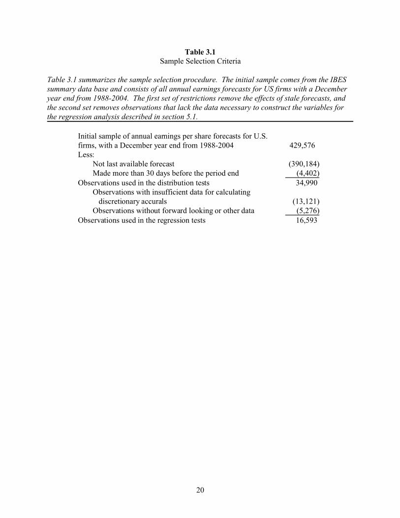
observations. I refer to this set of observations as the ‘restricted sample.’ Table 3.1 contains a

summary of the sample selection procedure.

3.2 Summary Statistics

Tables 3.2, 3.3, and 3.4 present summary counts and statistics for both the full and

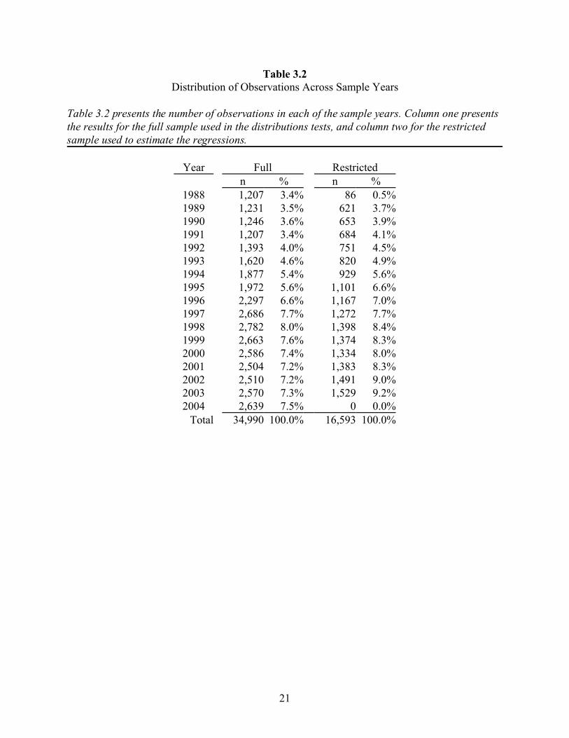
restricted samples. Table 3.2 presents a breakdown of the number of observations by year.

Column one presents the results for the full sample and column two for the restricted sample.

Although the distributions are similar, two differences should be mentioned. First, the restricted

sample has a smaller percentage of observations from 1988 than the full sample (0.5% versus

3.4%). This difference is most likely due to missing data in the Compustat database, since 1988

was the first year in which the cash flow data required for the calculation of discretionary

accruals was available. Second, the restricted sample has no observations in 2004. This is due to

the additional requirement that all observations in the restricted sample have earnings and analyst

forecast data for the upcoming year. For the remainder of the distribution, the samples follow a

similar pattern. More specifically, both samples show a relatively steady increase through 1998.

After 1998, the number of observations drops slightly, then slowly begins to increase. The

similarity of the two distributions suggests that the additional sample screens used to create the

restricted sample do not introduce differential bias across the sample years.

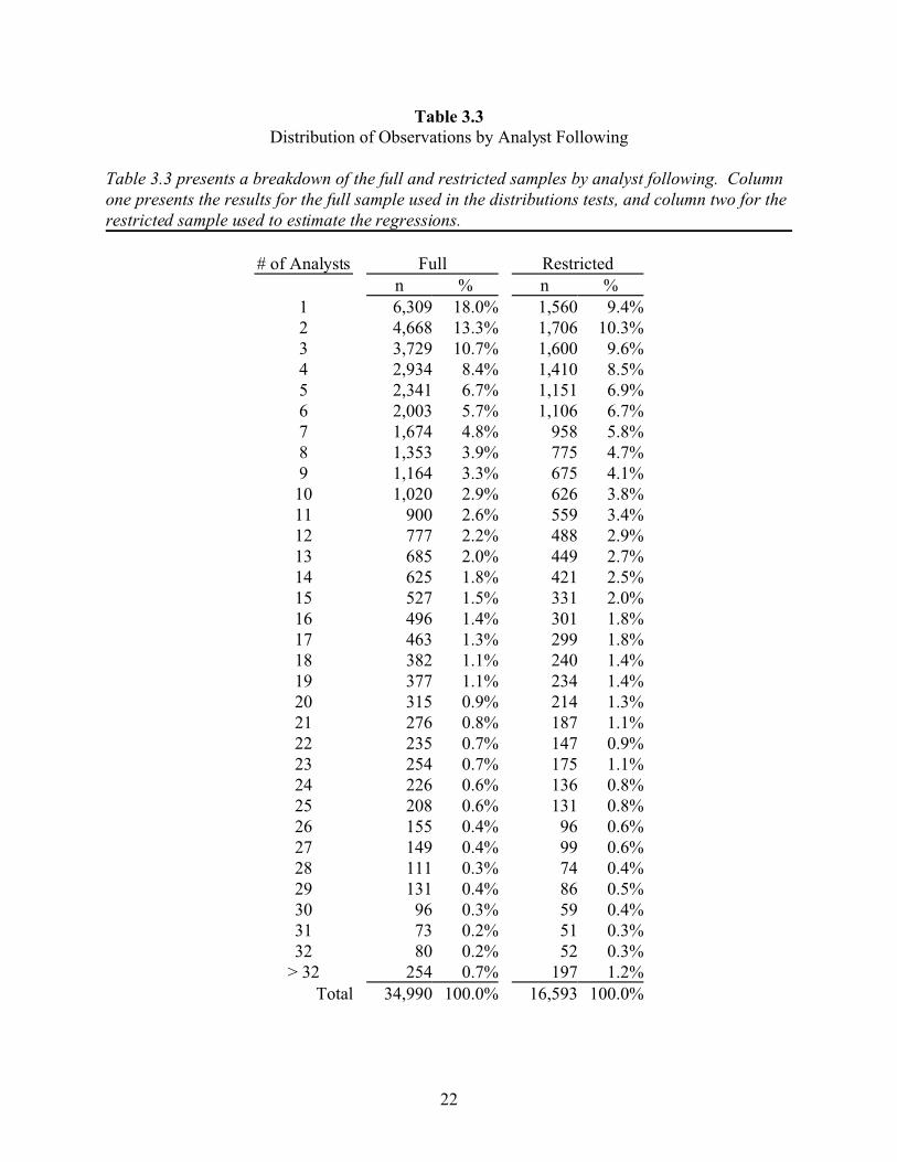
Table 3.3 presents an analysis of analyst following. Interestingly, the full sample shows

that many ‘consensus’ forecasts were made by only one analyst. The main difference between

the full and restricted samples is that fewer firms in the restricted sample are followed by only

17

one analyst. This is most likely due to the forward looking data requirement in the restricted

sample, because analyst coverage is likely to be more sporadic for firms followed by only one

analyst. Through the remainder of the distribution, both samples follow a gently decreasing

curve. As with the yearly breakdown, the overall similarity between the distributions suggests

that the sample screens do not introduce differential bias across the levels of analyst following.

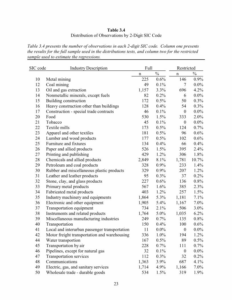
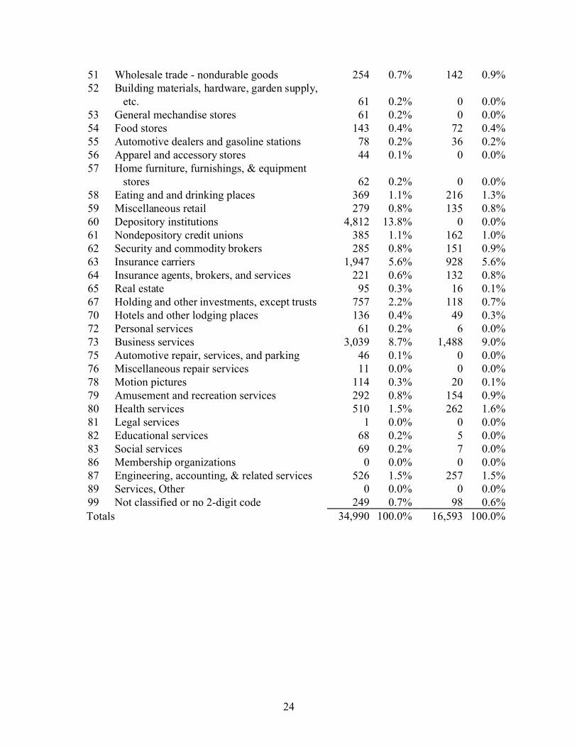
Table 3.4 presents the distribution of observations by 2-digit SIC code. Again, the

general industry representation is consistent between the full and restricted samples. The only

exception is the lack of depository institutions (SIC code 60) in the restricted sample compared to

a large number of these observations in the full sample. However, it is necessary to remove

financial institutions from the restricted sample in order to estimate discretionary accruals using

the Jones’ (1991) model. The similarities suggest that the sample screens do not introduce

differential bias across SIC codes, except where necessary to calculate the modified-Jones model

(see section 5.4 for more details).

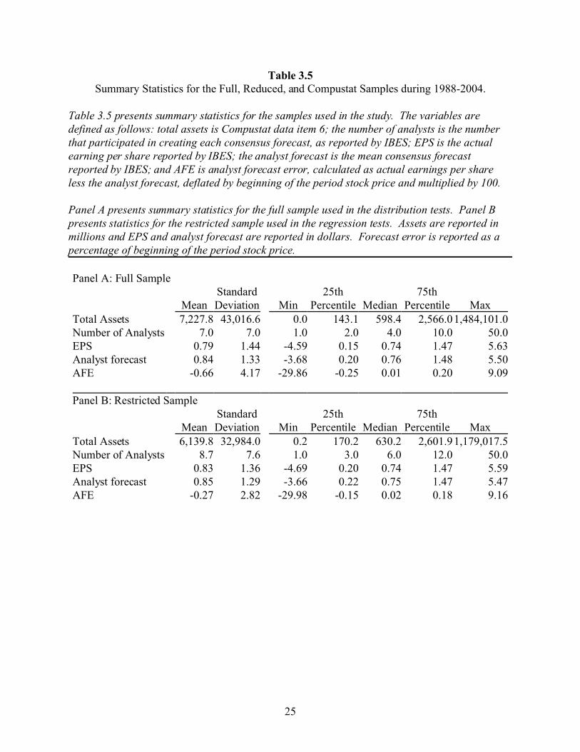
Table 3.5 presents summary statistics for the samples. The variables are defined as

follows: total assets is Compustat data item 6; the number of analysts is the number that

participated in creating each consensus forecast, as reported by IBES; EPS is the actual earnings

per share reported by IBES; the analyst forecast is the mean consensus forecast reported by IBES;

and analyst forecast error is actual earnings per share less the consensus analyst forecast, deflated

by beginning of the period stock price and multiplied by 100. Panel A of table 3.5 presents

statistics for the full sample and panel B presents results for the restricted sample. Several points

are noted. First, the full sample consists of larger firms than the restricted sample (average total

assets of $7,227.8 versus $6,139.8 million; p < 0.001 for a two-tailed test of the difference,

18

untabulated). Second, the analyst following is lower for the full sample than for the restricted

sample (average analyst following of 7 versus 8.7; p < 0.001).

In addition, table 3.5 provides preliminary evidence regarding the findings of Abarbanell

and Lehavy (2003) and Burgstahler and Eames (2003). Abarbanell and Lehavy (2003) find

evidence of the two asymmetries in the analyst forecast error distribution. First, they find a

higher than expected number of small positive forecast errors caused by a number of firms

meeting-or-beating earnings by a small amount, and second they find evidence of a longer and

thicker left tail caused by a group of firms reporting earnings considerably lower than the analyst

forecast. These patterns are consistent with earnings management and suggest that analysts are

omitting earnings management from their forecasts. Supporting this, I find that the mean analyst

forecast error is significantly negative for both samples (p < 0.001, untabulated) although the

medians are significantly positive (p < 0.001). Similarly, the negative tail is larger than the

positive tail, as shown by the more extreme values of the 25th percentile and minimum relative to

the values of the 75th percentile and maximum.

Burgstahler and Eames (2003) find that the distributions of earnings and analyst forecasts

are similar, with both including a chink above zero identified by prior research as evidence of

earnings management (Burgstahler and Dichev 1997). This suggests that analysts include the

effects of earnings management in their forecasts. However, I find that the mean earnings per

share is significantly smaller than the mean analyst forecast in both the full and restricted

samples (p-value for the two-tailed test of the difference is <0.001 and 0.051, respectively).

Similarly, the median, percentile, minimum and maximum of the analyst forecast distribution

appear to be larger than the earnings per share distribution. These differences are inconsistent

with the findings of Burgstahler and Eames (2003). On the other hand, the positive 25th

19

percentile, mean, and median values indicate a chink above zero in the distributions of both

earnings and analysts forecasts, consistent with the findings of Burgstahler and Eames (2003).

Chapter four will discuss the properties of the earnings, analyst forecast, and analyst forecast

error distributions in greater detail.

20

Table 3.1Sample Selection Criteria

Table 3.1 summarizes the sample selection procedure. The initial sample comes from the IBESsummary data base and consists of all annual earnings forecasts for US firms with a Decemberyear end from 1988-2004. The first set of restrictions remove the effects of stale forecasts, andthe second set removes observations that lack the data necessary to construct the variables forthe regression analysis described in section 5.1.

Initial sample of annual earnings per share forecasts for U.S. firms, with a December year end from 1988-2004 429,576Less:

Not last available forecast (390,184)Made more than 30 days before the period end (4,402)

Observations used in the distribution tests 34,990 Observations with insufficient data for calculating discretionary accurals (13,121)Observations without forward looking or other data (5,276)

Observations used in the regression tests 16,593

21

Table 3.2Distribution of Observations Across Sample Years

Table 3.2 presents the number of observations in each of the sample years. Column one presentsthe results for the full sample used in the distributions tests, and column two for the restrictedsample used to estimate the regressions.

Year Full Restrictedn % n %

1988 1,207 3.4% 86 0.5%1989 1,231 3.5% 621 3.7%1990 1,246 3.6% 653 3.9%1991 1,207 3.4% 684 4.1%1992 1,393 4.0% 751 4.5%1993 1,620 4.6% 820 4.9%1994 1,877 5.4% 929 5.6%1995 1,972 5.6% 1,101 6.6%1996 2,297 6.6% 1,167 7.0%1997 2,686 7.7% 1,272 7.7%1998 2,782 8.0% 1,398 8.4%1999 2,663 7.6% 1,374 8.3%2000 2,586 7.4% 1,334 8.0%2001 2,504 7.2% 1,383 8.3%2002 2,510 7.2% 1,491 9.0%2003 2,570 7.3% 1,529 9.2%2004 2,639 7.5% 0 0.0%

Total 34,990 100.0% 16,593 100.0%

22

Table 3.3Distribution of Observations by Analyst Following

Table 3.3 presents a breakdown of the full and restricted samples by analyst following. Columnone presents the results for the full sample used in the distributions tests, and column two for therestricted sample used to estimate the regressions.

# of Analysts Full Restrictedn % n %

1 6,309 18.0% 1,560 9.4%2 4,668 13.3% 1,706 10.3%3 3,729 10.7% 1,600 9.6%4 2,934 8.4% 1,410 8.5%5 2,341 6.7% 1,151 6.9%6 2,003 5.7% 1,106 6.7%7 1,674 4.8% 958 5.8%8 1,353 3.9% 775 4.7%9 1,164 3.3% 675 4.1%10 1,020 2.9% 626 3.8%11 900 2.6% 559 3.4%12 777 2.2% 488 2.9%13 685 2.0% 449 2.7%14 625 1.8% 421 2.5%15 527 1.5% 331 2.0%16 496 1.4% 301 1.8%17 463 1.3% 299 1.8%18 382 1.1% 240 1.4%19 377 1.1% 234 1.4%20 315 0.9% 214 1.3%21 276 0.8% 187 1.1%22 235 0.7% 147 0.9%23 254 0.7% 175 1.1%24 226 0.6% 136 0.8%25 208 0.6% 131 0.8%26 155 0.4% 96 0.6%27 149 0.4% 99 0.6%28 111 0.3% 74 0.4%29 131 0.4% 86 0.5%30 96 0.3% 59 0.4%31 73 0.2% 51 0.3%32 80 0.2% 52 0.3%

> 32 254 0.7% 197 1.2%Total 34,990 100.0% 16,593 100.0%

23

Table 3.4Distribution of Observations by 2-Digit SIC Code

Table 3.4 presents the number of observations in each 2-digit SIC code. Column one presentsthe results for the full sample used in the distributions tests, and column two for the restrictedsample used to estimate the regressions.

SIC code Industry Description Full Restrictedn % n %

10 Metal mining 225 0.6% 146 0.9%12 Coal mining 49 0.1% 7 0.0%13 Oil and gas extraction 1,157 3.3% 696 4.2%14 Nonmetallic minerals, except fuels 82 0.2% 6 0.0%15 Building construction 172 0.5% 50 0.3%16 Heavy construction other than buildings 128 0.4% 54 0.3%17 Construction - special trade contracts 46 0.1% 0 0.0%20 Food 530 1.5% 333 2.0%21 Tobacco 45 0.1% 0 0.0%22 Textile mills 173 0.5% 124 0.7%23 Apparel and other textiles 181 0.5% 96 0.6%24 Lumber and wood products 177 0.5% 102 0.6%25 Furniture and fixtures 134 0.4% 66 0.4%26 Paper and allied products 526 1.5% 395 2.4%27 Printing and publishing 429 1.2% 306 1.8%28 Chemicals and allied products 2,849 8.1% 1,781 10.7%29 Petroleum and coal products 328 0.9% 233 1.4%30 Rubber and miscellaneous plastic products 329 0.9% 207 1.2%31 Leather and leather products 95 0.3% 37 0.2%32 Stone, clay, and glass products 227 0.6% 136 0.8%33 Primary metal products 567 1.6% 385 2.3%34 Fabricated metal products 403 1.2% 257 1.5%35 Industry machinery and equipments 1,864 5.3% 1,181 7.1%36 Electronic and other equipment 1,905 5.4% 1,167 7.0%37 Transportation equipment 734 2.1% 506 3.0%38 Instruments and related products 1,764 5.0% 1,035 6.2%39 Miscellaneous manufacturing industries 249 0.7% 135 0.8%40 Transportation 150 0.4% 100 0.6%41 Local and interurban passenger transportation 11 0.0% 0 0.0%42 Motor freight transportation and warehousing 336 1.0% 194 1.2%44 Water transportion 167 0.5% 89 0.5%45 Transportation by air 228 0.7% 111 0.7%46 Pipelines, except for natural gas 32 0.1% 0 0.0%47 Transportation services 112 0.3% 32 0.2%48 Communications 1,363 3.9% 687 4.1%49 Electric, gas, and sanitary services 1,714 4.9% 1,166 7.0%50 Wholesale trade - durable goods 534 1.5% 319 1.9%

24

51 Wholesale trade - nondurable goods 254 0.7% 142 0.9%52 Building materials, hardware, garden supply,

etc. 61 0.2% 0 0.0%53 General mechandise stores 61 0.2% 0 0.0%54 Food stores 143 0.4% 72 0.4%55 Automotive dealers and gasoline stations 78 0.2% 36 0.2%56 Apparel and accessory stores 44 0.1% 0 0.0%57 Home furniture, furnishings, & equipment

stores 62 0.2% 0 0.0%58 Eating and and drinking places 369 1.1% 216 1.3%59 Miscellaneous retail 279 0.8% 135 0.8%60 Depository institutions 4,812 13.8% 0 0.0%61 Nondepository credit unions 385 1.1% 162 1.0%62 Security and commodity brokers 285 0.8% 151 0.9%63 Insurance carriers 1,947 5.6% 928 5.6%64 Insurance agents, brokers, and services 221 0.6% 132 0.8%65 Real estate 95 0.3% 16 0.1%67 Holding and other investments, except trusts 757 2.2% 118 0.7%70 Hotels and other lodging places 136 0.4% 49 0.3%72 Personal services 61 0.2% 6 0.0%73 Business services 3,039 8.7% 1,488 9.0%75 Automotive repair, services, and parking 46 0.1% 0 0.0%76 Miscellaneous repair services 11 0.0% 0 0.0%78 Motion pictures 114 0.3% 20 0.1%79 Amusement and recreation services 292 0.8% 154 0.9%80 Health services 510 1.5% 262 1.6%81 Legal services 1 0.0% 0 0.0%82 Educational services 68 0.2% 5 0.0%83 Social services 69 0.2% 7 0.0%86 Membership organizations 0 0.0% 0 0.0%87 Engineering, accounting, & related services 526 1.5% 257 1.5%89 Services, Other 0 0.0% 0 0.0%99 Not classified or no 2-digit code 249 0.7% 98 0.6%Totals 34,990 100.0% 16,593 100.0%

25

Table 3.5Summary Statistics for the Full, Reduced, and Compustat Samples during 1988-2004.

Table 3.5 presents summary statistics for the samples used in the study. The variables aredefined as follows: total assets is Compustat data item 6; the number of analysts is the numberthat participated in creating each consensus forecast, as reported by IBES; EPS is the actualearning per share reported by IBES; the analyst forecast is the mean consensus forecastreported by IBES; and AFE is analyst forecast error, calculated as actual earnings per shareless the analyst forecast, deflated by beginning of the period stock price and multiplied by 100.

Panel A presents summary statistics for the full sample used in the distribution tests. Panel Bpresents statistics for the restricted sample used in the regression tests. Assets are reported inmillions and EPS and analyst forecast are reported in dollars. Forecast error is reported as apercentage of beginning of the period stock price.

Panel A: Full SampleStandard 25th 75th

Mean Deviation Min Percentile Median Percentile MaxTotal Assets 7,227.8 43,016.6 0.0 143.1 598.4 2,566.01,484,101.0Number of Analysts 7.0 7.0 1.0 2.0 4.0 10.0 50.0EPS 0.79 1.44 -4.59 0.15 0.74 1.47 5.63Analyst forecast 0.84 1.33 -3.68 0.20 0.76 1.48 5.50AFE -0.66 4.17 -29.86 -0.25 0.01 0.20 9.09 Panel B: Restricted Sample

Standard 25th 75thMean Deviation Min Percentile Median Percentile Max

Total Assets 6,139.8 32,984.0 0.2 170.2 630.2 2,601.91,179,017.5Number of Analysts 8.7 7.6 1.0 3.0 6.0 12.0 50.0EPS 0.83 1.36 -4.69 0.20 0.74 1.47 5.59Analyst forecast 0.85 1.29 -3.66 0.22 0.75 1.47 5.47AFE -0.27 2.82 -29.98 -0.15 0.02 0.18 9.16

26

CHAPTER 4

REPLICATIONS

4.1 Burgstahler and Eames (2003)

Burgstahler and Eames (2003) compare the distributions of earnings and analyst

forecasts, and observe a chink immediately above zero in both distributions. This chink is

caused by a higher number of small positive than small negative values, and was noted earlier by

Burgstahler and Dichev (1997) who interpreted it as evidence of earnings management.

Burgstahler and Eames observe that the distribution of analysts’ forecasts, including the size and

position of the chink, is almost identical to that of the earnings distribution, and conclude that

this is because analysts include the effects of earnings management in their forecasts.

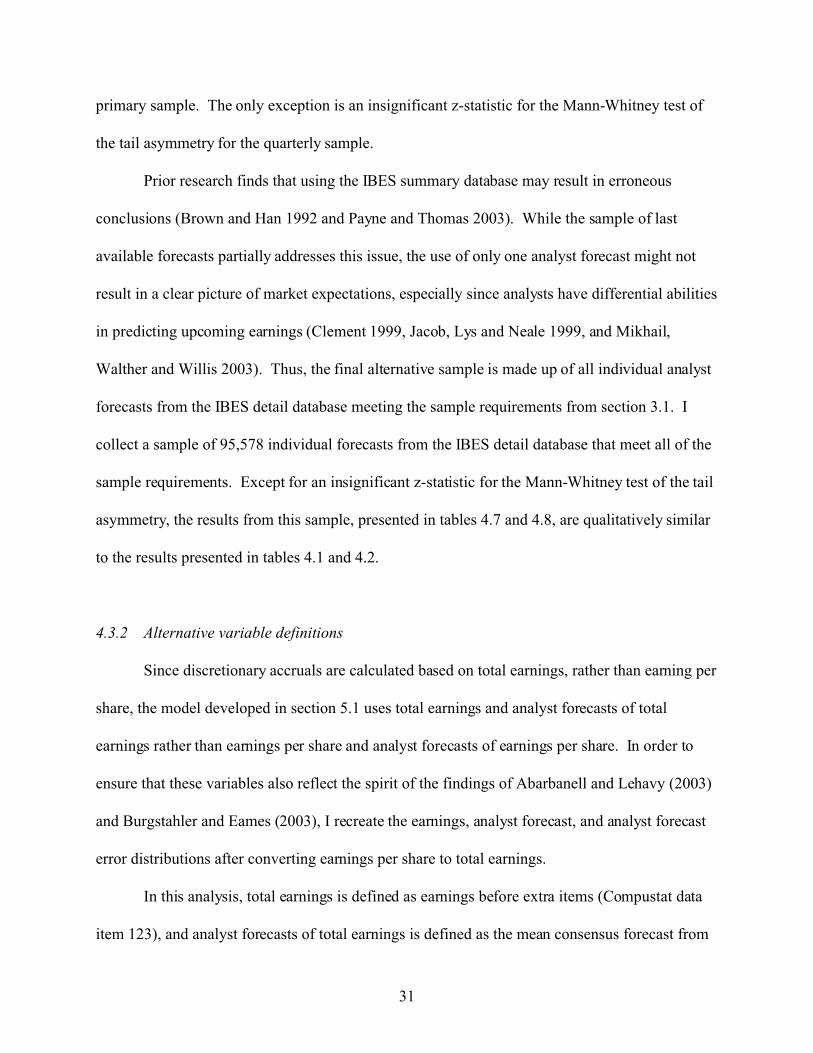
The distributions of earnings and analyst forecasts for my full sample of 34,990

observations are presented in figure 4.1. I define earnings as actual earnings reported by IBES

and analyst forecasts as the mean consensus forecast reported by IBES. Both variables are

deflated by the beginning of the period stock price. As in Burgstahler and Eames (2003), the two

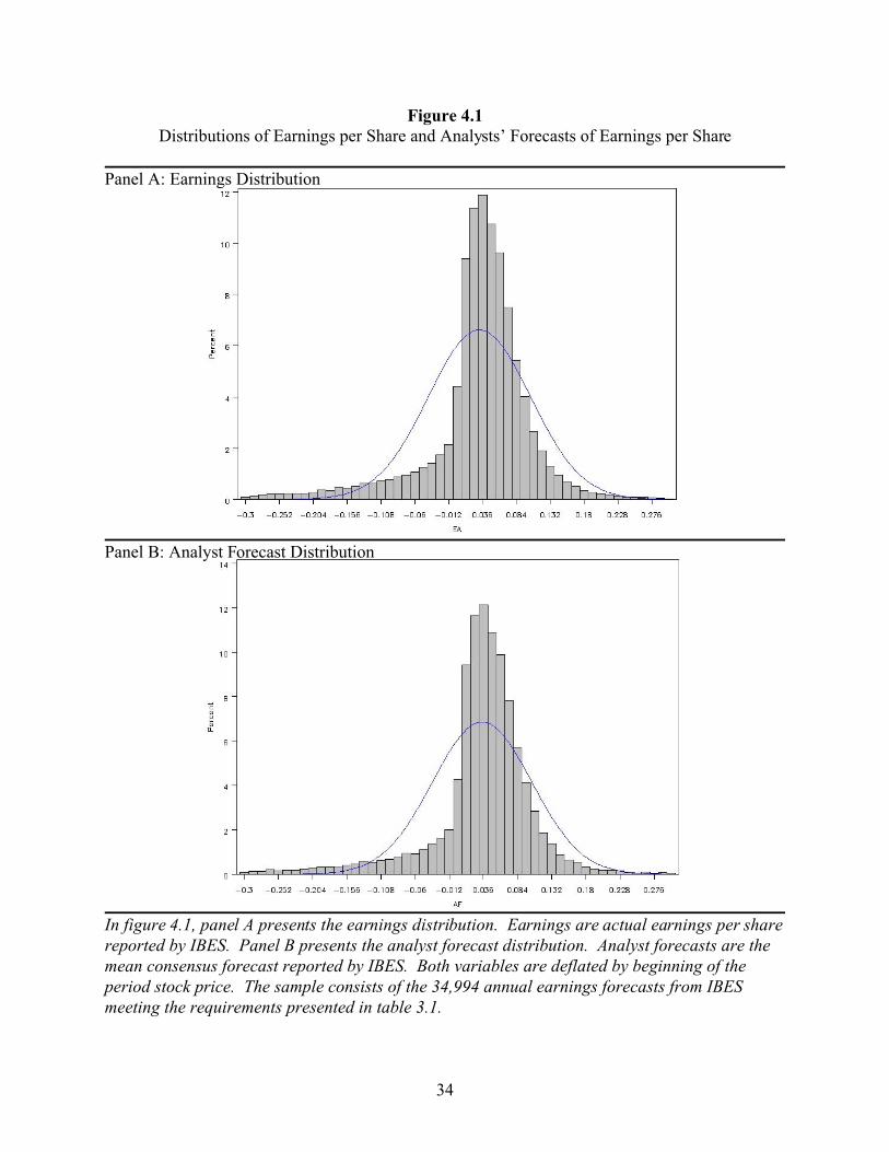
distributions are similar, with an obvious chink above zero. The analysis in table 4.1 confirms

the statistical significance of the chinks. Column one presents the results of chi-square tests that

compare the number of observations in various bins above zero to the number of observations in

the corresponding bins below zero. Column two of table 4.1 presents the percentage of

observations that fall into each concentric set of bins (that is, the total number of observations

used to calculate the ratio presented in column one). Consistent with the visual and statistical

27

evidence of the chink, the majority of observations fall within the [-0.1, 0.1] range and are mostly

positive, as shown by the ratio presented in column one.

A comparison of the results in panels A and B of table 4.1 reveals further similarities

between the two distributions. The percentages listed in column two are almost identical for the

two distributions, and the pattern of the ratios of positive to negative observations in each set of

bins, presented in column one, is also similar. However, the analyst forecast distribution shows

greater evidence of the chink than does the earnings distribution, as shown by the higher value of

the ratios presented in column one of panel B. This evidence is consistent with Burgstahler and

Eames’ (2003, page 256) conjecture that analysts sometimes anticipate earnings management that

does not materialize.

4.2 Abarbanell and Lehavy (2003)

Abarbanell and Lehavy (2003) observe that prior evidence of analyst optimism (see, for

example, Kadous, Kirsche and Sedor 2004) is not consistent with analysts’ incentives. For

example, analysts who want to encourage managers to provide them with additional information

are unlikely to antagonize them by issuing a forecast that managers cannot reach. In an attempt

to explain this phenomenon, Abarbanell and Lehavy (2003) examine the distribution of analyst

forecast errors. They find two asymmetries. First, although a considerable number of firms just

beat the consensus analyst forecast, there is no corresponding group that just misses the forecast.

This causes a chink in the distribution above zero. Abarbanell and Lehavy refer to this as the

middle asymmetry. Second, although a group of firms misses the consensus analyst forecast by a

large amount, few, if any, beat the forecast by a large amount. This causes the left tail of the

distribution to be longer and thicker than the right tail. Abarbanell and Lehavy refer to this as the

28

tail asymmetry. These asymmetries could be caused by earnings management to either meet-or-

beat the forecast or to take a ‘big bath’ when the forecast cannot be met. In additional tests,

Abarbanell and Lehavy (2003) find that the firms that create these asymmetries have higher

levels of discretionary accruals, another clue that earnings management could be taking place.

Based on these results, they conclude that analysts omit the effects of earnings management when

issuing their earnings forecasts.

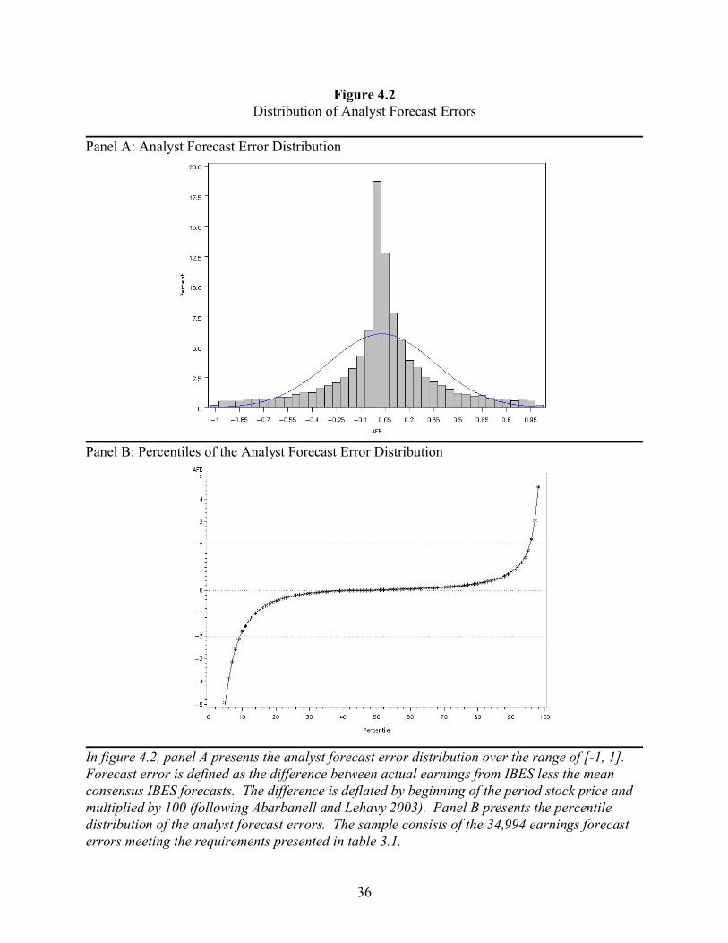
The forecast error distribution for my sample is presented in figure 4.2, panel A.

I define analyst forecast error as earnings reported by IBES less the mean consensus forecast,

deflated by beginning of the period stock price and multiplied by 100. This definition is

consistent with Abarbanell and Lehavy (2003). Visual inspection shows a chink above zero,

consistent with the findings of Abarbanell and Lehavy (2003). Panel B of figure 4.2 presents a

graph of the percentiles of the distribution, which provides a clearer picture of the tails of the

distribution. I observe a longer and thicker left tail, consistent with Abarbanell and Lehavy’s

(2003) tail asymmetry.

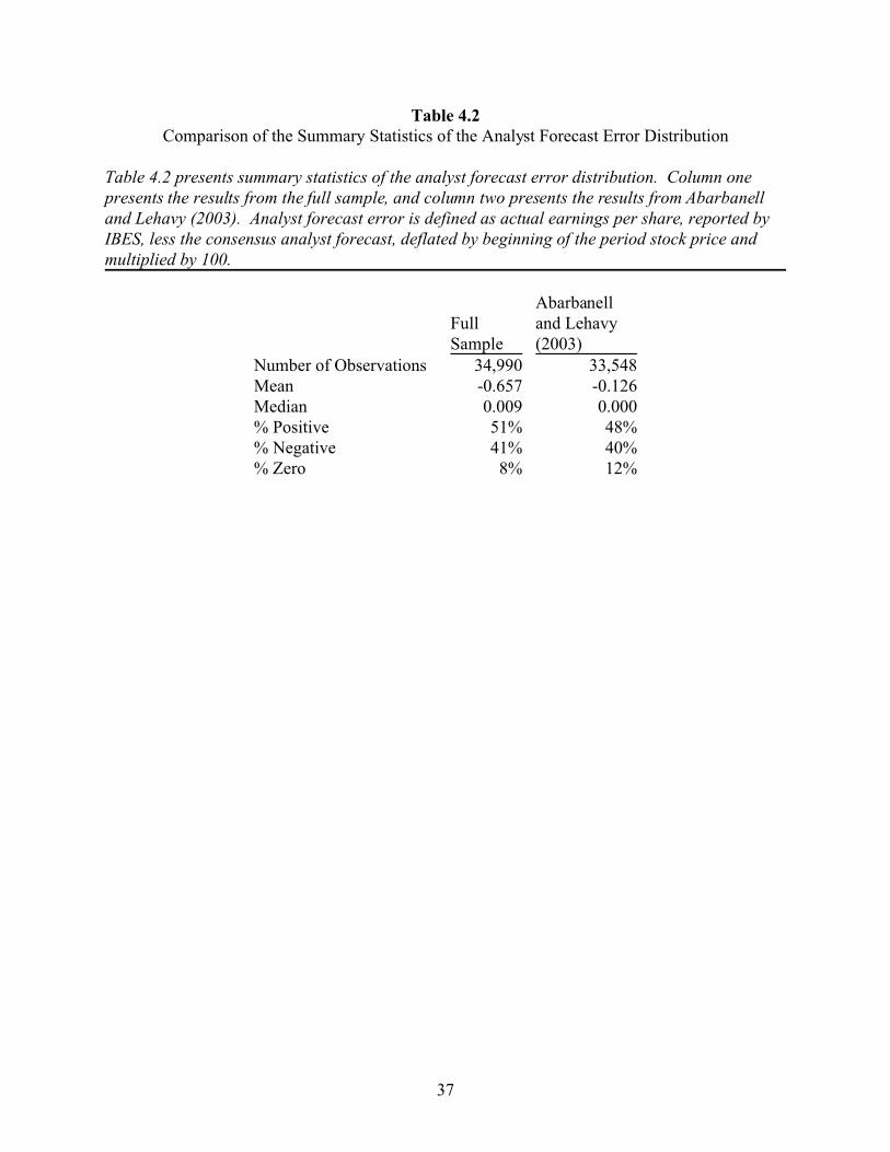
Table 4.2, column one, presents summary statistics for the analyst forecast error

distribution from my sample and column two presents corresponding results from Abarbanell and

Lehavy’s (2003) sample. Although a direct comparison of the results is difficult due to

differences in the sample selection criteria, the summary statistics appear to be consistent

between the two studies. The breakdown of positive, negative, and zero analyst forecast errors is

similar, as is the size of the samples. In addition, both samples have a negative mean analyst

forecast error and a median forecast error that is either zero or close to zero. The most notable

difference is the relative size of mean analyst forecast error, which is most likely caused by the

more extreme negative values in the left tail of the full sample (shown in panel A of table 4.3). I

29

attribute this to the fact that my sample is made up annual forecasts and Abarbanell and Lehavy

(2003) use quarterly forecasts. Column three of table 4.6 presents the results for a sample of

quarterly analyst forecast errors (discussed below). The mean analyst forecast errors and

percentile values for that sample are closer to those reported by Abarbanell and Lehavy (2003).

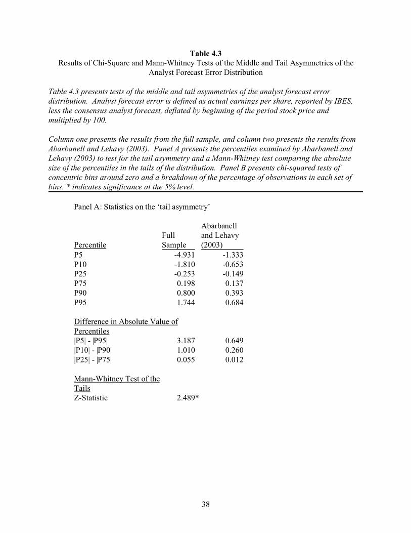
Panel A of table 4.3 presents the percentiles of the forecast error distribution and the

results of a Mann Whitney test of the tail asymmetry. Column one presents the results for the

full sample and column two from Abarbanell and Lehavy (2003). The Mann Whitney test

compares the absolute values of the 1st through 10th percentiles (the left tail) to those of the 90th

through 99th percentiles (the right tail) of the distribution. Under the null hypothesis of a

symmetric distribution, the amounts should be identical. I find a significant z-statistic, which

indicates that one tail is longer and thicker than the other. An examination of the percentiles and

the difference in corresponding percentiles confirms that the left tail is larger than the right tail.

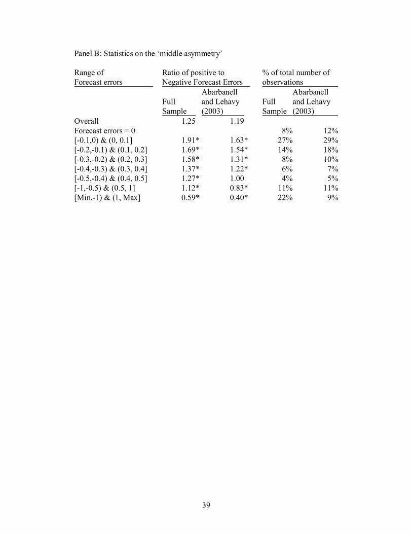
Panel B, column one, presents chi-squared tests of the number of positive to negative

observations in concentric bins around zero to test the significance of the chink above zero. The

results are consistent with the visual evidence in figure 4.2. In addition, column two presents the

percentages of observations falling into each set of bins. The higher percentage of observations

in the bins around zero, the majority of which are positive, provides additional support for

existence of the middle asymmetry.

4.3 Sensitivity Tests

4.3.1 Alternative samples

The tests reported here do not provide a direct replication of Abarbanell and Lehavy

(2003) and Burgstahler and Eames (2003) because the samples vary between studies. Although

6The results from the quarterly sample are reported separately because the bin sizes forthe chi-squared tests are smaller than those used for the median and last available forecastsamples. This is due to the smaller size of the quarterly earnings announcements relative toannual earnings.

30

the similarities in the results presented in sections 4.1 and 4.2 to those of Abarbanell and Lehavy

(2003) and Burgstahler and Eames (2003) reduce this concern, I replicate my results using the

median consensus forecast, the last available forecast (both consistent with Burgstahler and

Eames 2003) and a sample of quarterly consensus forecasts (consistent with Abarbanell and

Lehavy 2003). The median consensus forecast sample (n = 34,990) is constructed by substituting

the median forecast for the mean forecast in the full sample. The last available forecast (n =

9,698) and quarterly consensus forecast (n = 128,612) samples are constructed using a sample of

individual annual and consensus quarterly forecasts, respectively. All of the sample screens

discussed in section 3.1 are then applied. For all three alternative samples, the distributions are

similar to those presented in figures 4.1 and 4.2.

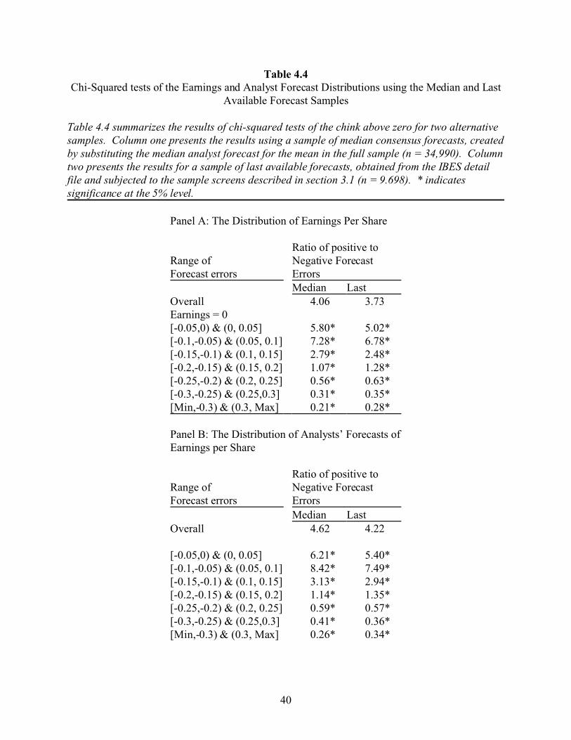
Table 4.4 presents the results of chi-squared tests of the middle asymmetry for the median

and last available forecast samples. As in table 4.1, panel A presents results for the earnings

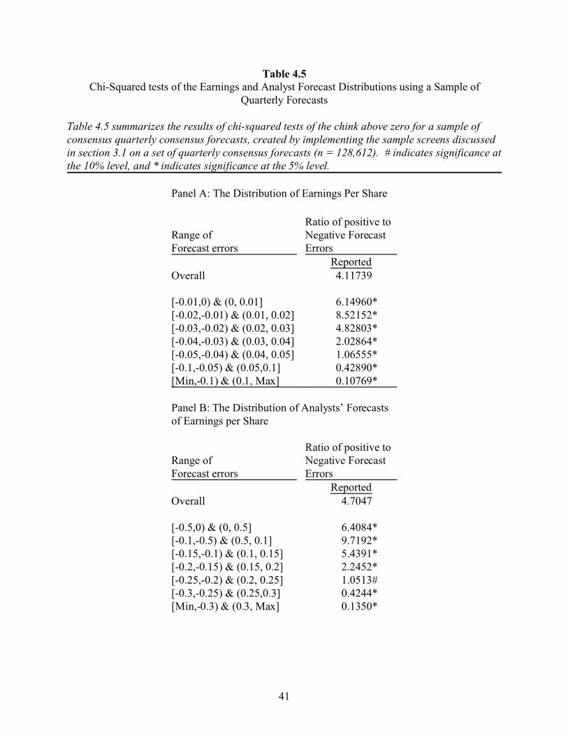
distributions, while panel B presents results for the analyst forecast distributions. Table 4.5

presents analogous results using the sample of quarterly observations.6 The results using these

alternative samples are qualitatively similar to those presented in table 4.1.

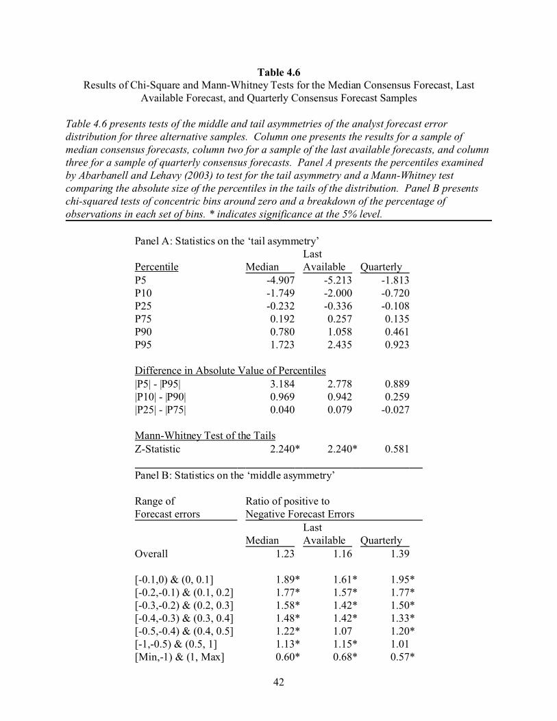
Table 4.6 presents the tests for the two asymmetries in the analyst forecast error

distribution for the three alternative samples. Column one presents the results for the median

analyst forecast sample, column two for the last available forecast sample, and column three for

the quarterly forecast sample. In each case, the findings are consistent with those from the

31

primary sample. The only exception is an insignificant z-statistic for the Mann-Whitney test of

the tail asymmetry for the quarterly sample.

Prior research finds that using the IBES summary database may result in erroneous

conclusions (Brown and Han 1992 and Payne and Thomas 2003). While the sample of last

available forecasts partially addresses this issue, the use of only one analyst forecast might not

result in a clear picture of market expectations, especially since analysts have differential abilities

in predicting upcoming earnings (Clement 1999, Jacob, Lys and Neale 1999, and Mikhail,

Walther and Willis 2003). Thus, the final alternative sample is made up of all individual analyst

forecasts from the IBES detail database meeting the sample requirements from section 3.1. I

collect a sample of 95,578 individual forecasts from the IBES detail database that meet all of the

sample requirements. Except for an insignificant z-statistic for the Mann-Whitney test of the tail

asymmetry, the results from this sample, presented in tables 4.7 and 4.8, are qualitatively similar

to the results presented in tables 4.1 and 4.2.

4.3.2 Alternative variable definitions

Since discretionary accruals are calculated based on total earnings, rather than earning per

share, the model developed in section 5.1 uses total earnings and analyst forecasts of total

earnings rather than earnings per share and analyst forecasts of earnings per share. In order to

ensure that these variables also reflect the spirit of the findings of Abarbanell and Lehavy (2003)

and Burgstahler and Eames (2003), I recreate the earnings, analyst forecast, and analyst forecast

error distributions after converting earnings per share to total earnings.

In this analysis, total earnings is defined as earnings before extra items (Compustat data

item 123), and analyst forecasts of total earnings is defined as the mean consensus forecast from

32

the IBES database multiplied by the total number of shares used to calculate EPS (Compustat

data item 54). Both of these variables are then deflated by total assets. The earnings and analyst

forecast distributions are shown in figure 4.3. As in figure 4.1, the distributions are almost

identical, especially with respect to the chink above zero.

Figure 4.4 presents the distributions of analyst forecast errors, where analyst forecast error

is defined as the difference between total earnings and the analyst forecast multiplied by the

number of shares used to calculate EPS, deflated by total assets. This definition of analyst

forecast error is used for comparison with the variables definitions used in figure 4.3. Panel A

presents the distribution of analyst forecast errors and provides visual evidence of the chink

above zero, consistent with the middle asymmetry. Panel B graphs the percentiles of the analyst

forecast error distribution. Although the graph shows a much tighter distribution than in panel B

of figure 4.2, there is still evidence that the left tail of the distribution is longer and thicker than

the right tail. These results suggest that an analysis based on total earnings can be used to

reconcile the results of Abarbanell and Lehavy (2003) and Burgstahler and Eames (2003).

4.3.3 Deflating

A recent study by Durtschi and Easton (2005) suggests that the evidence of a ‘chink’ in

the earnings distribution is caused by the use of stock price as a deflator, rather than earnings

management (as proposed by Burgstahler and Dichev 1997). They theorize that firms meeting-

or-beating their benchmarks will have a higher stock price than firms missing their benchmarks.

This will lead to larger denominators for the meet-or-beat firms and, consequently, will pull

observations into the bins immediately above zero without any earnings management. Firms that

miss the benchmarks, on the other hand, will have smaller denominators, which will tend to push

33

the observations away from zero. In order to address the possibility that the results from the

primary tests are caused by deflating, I replicated the tests without deflating by stock price. The

results, presented in figures 4.5 and 4.6 are qualitatively similar to those presented in figures 4.1

and 4.2.

4.4 Summary

The similarities in the earnings and analyst forecast distributions suggest that analysts

include the effects of earnings management when issuing their forecasts, consistent with the

findings of Burgstahler and Eames (2003). Based on this finding, I would expect the analyst

forecast errors to be caused by only random error, leading to an analyst forecast error distribution

that is symmetric around zero. Instead, the forecast error distribution has its own chink above

zero and a fat left tail, consistent with the findings of Abarbanell and Lehavy (2003), who claim

that analysts remove the effects of earnings management from their forecasts. In the next chapter

I attempt to resolve this discrepancy.

34

Figure 4.1Distributions of Earnings per Share and Analysts’ Forecasts of Earnings per Share

Panel A: Earnings Distribution

Panel B: Analyst Forecast Distribution

In figure 4.1, panel A presents the earnings distribution. Earnings are actual earnings per sharereported by IBES. Panel B presents the analyst forecast distribution. Analyst forecasts are themean consensus forecast reported by IBES. Both variables are deflated by beginning of theperiod stock price. The sample consists of the 34,994 annual earnings forecasts from IBESmeeting the requirements presented in table 3.1.

35

Table 4.1Results of Chi-Square Tests of the Ratio of Positive to Negative Observations in the

Distributions of Earnings and Analyst Forecasts

Table 4.1 presents tests of the statistical significance of the chink above zero for the earningsand analyst forecast distributions. Panel A presents the results for the earnings distribution andpanel B for the analyst forecast distribution. The first column presents the ratio of positive tonegative observations falling in concentric bins around 0. A chi-squared test is used todetermine if there is a significant difference in the number of positive and negative observations.* indicates significance at the 5% level. In column two presents the percentage of observationsfalling in each bin width. A significant chink above zero is evidenced by a high percentage ofobservations falling close to zero.

Panel A: The Distribution of Earnings Per Share

Range of Ratio of positive to % of total number ofForecast errors Negative Forecast Errors observations

Reported ReportedOverall 4.06Earnings per Share = 0 0%[-0.05,0) & (0, 0.05] 5.80* 49%[-0.1,-0.05) & (0.05, 0.1] 7.28* 32%[-0.15,-0.1) & (0.1, 0.15] 2.79* 10%[-0.2,-0.15) & (0.15, 0.2] 1.07* 3%[-0.25,-0.2) & (0.2, 0.25] 0.56* 2%[-0.3,-0.25) & (0.25,0.3] 0.31* 1%[Min,-0.3) & (0.3, Max] 0.21* 4%

Panel B: The Distribution of Analysts’ Forecasts of Earnings per Share

Range of Ratio of positive to % of total number ofForecast errors Negative Forecast Errors observations

Reported ReportedOverall 4.62Forecast = 0 0%[-0.05,0) & (0, 0.05] 6.18* 49%[-0.1,-0.05) & (0.05, 0.1] 8.51* 33%[-0.15,-0.1) & (0.1, 0.15] 3.08* 10%[-0.2,-0.15) & (0.15, 0.2] 1.12* 3%[-0.25,-0.2) & (0.2, 0.25] 0.61* 1%[-0.3,-0.25) & (0.25,0.3] 0.42* 1%[Min,-0.3) & (0.3, Max] 0.26* 3%

36

Figure 4.2Distribution of Analyst Forecast Errors

Panel A: Analyst Forecast Error Distribution

Panel B: Percentiles of the Analyst Forecast Error Distribution

In figure 4.2, panel A presents the analyst forecast error distribution over the range of [-1, 1]. Forecast error is defined as the difference between actual earnings from IBES less the meanconsensus IBES forecasts. The difference is deflated by beginning of the period stock price andmultiplied by 100 (following Abarbanell and Lehavy 2003). Panel B presents the percentiledistribution of the analyst forecast errors. The sample consists of the 34,994 earnings forecasterrors meeting the requirements presented in table 3.1.

37

Table 4.2Comparison of the Summary Statistics of the Analyst Forecast Error Distribution

Table 4.2 presents summary statistics of the analyst forecast error distribution. Column onepresents the results from the full sample, and column two presents the results from Abarbanelland Lehavy (2003). Analyst forecast error is defined as actual earnings per share, reported byIBES, less the consensus analyst forecast, deflated by beginning of the period stock price andmultiplied by 100.

FullSample

Abarbanelland Lehavy(2003)

Number of Observations 34,990 33,548Mean -0.657 -0.126Median 0.009 0.000% Positive 51% 48%% Negative 41% 40%% Zero 8% 12%

38

Table 4.3Results of Chi-Square and Mann-Whitney Tests of the Middle and Tail Asymmetries of the

Analyst Forecast Error Distribution

Table 4.3 presents tests of the middle and tail asymmetries of the analyst forecast errordistribution. Analyst forecast error is defined as actual earnings per share, reported by IBES,less the consensus analyst forecast, deflated by beginning of the period stock price andmultiplied by 100.

Column one presents the results from the full sample, and column two presents the results fromAbarbanell and Lehavy (2003). Panel A presents the percentiles examined by Abarbanell andLehavy (2003) to test for the tail asymmetry and a Mann-Whitney test comparing the absolutesize of the percentiles in the tails of the distribution. Panel B presents chi-squared tests ofconcentric bins around zero and a breakdown of the percentage of observations in each set ofbins. * indicates significance at the 5% level.

Panel A: Statistics on the ‘tail asymmetry’

PercentileFullSample

Abarbanelland Lehavy(2003)

P5 -4.931 -1.333P10 -1.810 -0.653P25 -0.253 -0.149P75 0.198 0.137P90 0.800 0.393P95 1.744 0.684

Difference in Absolute Value ofPercentiles|P5| - |P95| 3.187 0.649|P10| - |P90| 1.010 0.260|P25| - |P75| 0.055 0.012

Mann-Whitney Test of theTailsZ-Statistic 2.489*

39

Panel B: Statistics on the ‘middle asymmetry’

Range of Ratio of positive to % of total number ofForecast errors Negative Forecast Errors observations

FullSample

Abarbanelland Lehavy(2003)

FullSample

Abarbanelland Lehavy(2003)

Overall 1.25 1.19Forecast errors = 0 8% 12%[-0.1,0) & (0, 0.1] 1.91* 1.63* 27% 29%[-0.2,-0.1) & (0.1, 0.2] 1.69* 1.54* 14% 18%[-0.3,-0.2) & (0.2, 0.3] 1.58* 1.31* 8% 10%[-0.4,-0.3) & (0.3, 0.4] 1.37* 1.22* 6% 7%[-0.5,-0.4) & (0.4, 0.5] 1.27* 1.00 4% 5%[-1,-0.5) & (0.5, 1] 1.12* 0.83* 11% 11%[Min,-1) & (1, Max] 0.59* 0.40* 22% 9%

40

Table 4.4Chi-Squared tests of the Earnings and Analyst Forecast Distributions using the Median and Last

Available Forecast Samples

Table 4.4 summarizes the results of chi-squared tests of the chink above zero for two alternativesamples. Column one presents the results using a sample of median consensus forecasts, createdby substituting the median analyst forecast for the mean in the full sample (n = 34,990). Columntwo presents the results for a sample of last available forecasts, obtained from the IBES detailfile and subjected to the sample screens described in section 3.1 (n = 9.698). * indicatessignificance at the 5% level.

Panel A: The Distribution of Earnings Per Share

Ratio of positive to Range ofForecast errors

Negative ForecastErrorsMedian Last

Overall 4.06 3.73Earnings = 0[-0.05,0) & (0, 0.05] 5.80* 5.02*[-0.1,-0.05) & (0.05, 0.1] 7.28* 6.78*[-0.15,-0.1) & (0.1, 0.15] 2.79* 2.48*[-0.2,-0.15) & (0.15, 0.2] 1.07* 1.28*[-0.25,-0.2) & (0.2, 0.25] 0.56* 0.63*[-0.3,-0.25) & (0.25,0.3] 0.31* 0.35*[Min,-0.3) & (0.3, Max] 0.21* 0.28*

Panel B: The Distribution of Analysts’ Forecasts ofEarnings per Share

Ratio of positive to Range ofForecast errors

Negative ForecastErrors

Median LastOverall 4.62 4.22

[-0.05,0) & (0, 0.05] 6.21* 5.40*[-0.1,-0.05) & (0.05, 0.1] 8.42* 7.49*[-0.15,-0.1) & (0.1, 0.15] 3.13* 2.94*[-0.2,-0.15) & (0.15, 0.2] 1.14* 1.35*[-0.25,-0.2) & (0.2, 0.25] 0.59* 0.57*[-0.3,-0.25) & (0.25,0.3] 0.41* 0.36*[Min,-0.3) & (0.3, Max] 0.26* 0.34*

41

Table 4.5Chi-Squared tests of the Earnings and Analyst Forecast Distributions using a Sample of

Quarterly Forecasts

Table 4.5 summarizes the results of chi-squared tests of the chink above zero for a sample ofconsensus quarterly consensus forecasts, created by implementing the sample screens discussedin section 3.1 on a set of quarterly consensus forecasts (n = 128,612). # indicates significance atthe 10% level, and * indicates significance at the 5% level.

Panel A: The Distribution of Earnings Per Share

Ratio of positive to Range ofForecast errors

Negative ForecastErrors

ReportedOverall 4.11739

[-0.01,0) & (0, 0.01] 6.14960*[-0.02,-0.01) & (0.01, 0.02] 8.52152*[-0.03,-0.02) & (0.02, 0.03] 4.82803*[-0.04,-0.03) & (0.03, 0.04] 2.02864*[-0.05,-0.04) & (0.04, 0.05] 1.06555*[-0.1,-0.05) & (0.05,0.1] 0.42890*[Min,-0.1) & (0.1, Max] 0.10769*

Panel B: The Distribution of Analysts’ Forecastsof Earnings per Share

Ratio of positive to Range ofForecast errors

Negative ForecastErrors

ReportedOverall 4.7047

[-0.5,0) & (0, 0.5] 6.4084*[-0.1,-0.5) & (0.5, 0.1] 9.7192*[-0.15,-0.1) & (0.1, 0.15] 5.4391*[-0.2,-0.15) & (0.15, 0.2] 2.2452*[-0.25,-0.2) & (0.2, 0.25] 1.0513#[-0.3,-0.25) & (0.25,0.3] 0.4244*[Min,-0.3) & (0.3, Max] 0.1350*

42

Table 4.6Results of Chi-Square and Mann-Whitney Tests for the Median Consensus Forecast, Last

Available Forecast, and Quarterly Consensus Forecast Samples

Table 4.6 presents tests of the middle and tail asymmetries of the analyst forecast errordistribution for three alternative samples. Column one presents the results for a sample ofmedian consensus forecasts, column two for a sample of the last available forecasts, and columnthree for a sample of quarterly consensus forecasts. Panel A presents the percentiles examinedby Abarbanell and Lehavy (2003) to test for the tail asymmetry and a Mann-Whitney testcomparing the absolute size of the percentiles in the tails of the distribution. Panel B presentschi-squared tests of concentric bins around zero and a breakdown of the percentage ofobservations in each set of bins. * indicates significance at the 5% level.

Panel A: Statistics on the ‘tail asymmetry’Last

Percentile Median Available QuarterlyP5 -4.907 -5.213 -1.813P10 -1.749 -2.000 -0.720P25 -0.232 -0.336 -0.108P75 0.192 0.257 0.135P90 0.780 1.058 0.461P95 1.723 2.435 0.923

Difference in Absolute Value of Percentiles|P5| - |P95| 3.184 2.778 0.889|P10| - |P90| 0.969 0.942 0.259|P25| - |P75| 0.040 0.079 -0.027

Mann-Whitney Test of the TailsZ-Statistic 2.240* 2.240* 0.581 Panel B: Statistics on the ‘middle asymmetry’

Range of Ratio of positive to Forecast errors Negative Forecast Errors

LastMedian Available Quarterly

Overall 1.23 1.16 1.39

[-0.1,0) & (0, 0.1] 1.89* 1.61* 1.95*[-0.2,-0.1) & (0.1, 0.2] 1.77* 1.57* 1.77*[-0.3,-0.2) & (0.2, 0.3] 1.58* 1.42* 1.50*[-0.4,-0.3) & (0.3, 0.4] 1.48* 1.42* 1.33*[-0.5,-0.4) & (0.4, 0.5] 1.22* 1.07 1.20*[-1,-0.5) & (0.5, 1] 1.13* 1.15* 1.01[Min,-1) & (1, Max] 0.60* 0.68* 0.57*

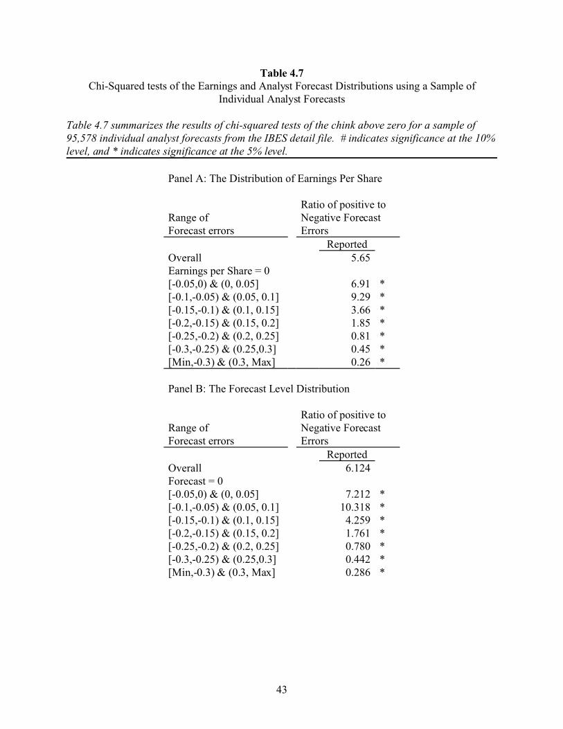
43

Table 4.7Chi-Squared tests of the Earnings and Analyst Forecast Distributions using a Sample of

Individual Analyst Forecasts

Table 4.7 summarizes the results of chi-squared tests of the chink above zero for a sample of95,578 individual analyst forecasts from the IBES detail file. # indicates significance at the 10%level, and * indicates significance at the 5% level.

Panel A: The Distribution of Earnings Per Share

Ratio of positive to Range ofForecast errors

Negative ForecastErrors

ReportedOverall 5.65Earnings per Share = 0[-0.05,0) & (0, 0.05] 6.91 *[-0.1,-0.05) & (0.05, 0.1] 9.29 *[-0.15,-0.1) & (0.1, 0.15] 3.66 *[-0.2,-0.15) & (0.15, 0.2] 1.85 *[-0.25,-0.2) & (0.2, 0.25] 0.81 *[-0.3,-0.25) & (0.25,0.3] 0.45 *[Min,-0.3) & (0.3, Max] 0.26 *

Panel B: The Forecast Level Distribution

Ratio of positive to Range ofForecast errors

Negative ForecastErrors

ReportedOverall 6.124Forecast = 0[-0.05,0) & (0, 0.05] 7.212 *[-0.1,-0.05) & (0.05, 0.1] 10.318 *[-0.15,-0.1) & (0.1, 0.15] 4.259 *[-0.2,-0.15) & (0.15, 0.2] 1.761 *[-0.25,-0.2) & (0.2, 0.25] 0.780 *[-0.3,-0.25) & (0.25,0.3] 0.442 *[Min,-0.3) & (0.3, Max] 0.286 *

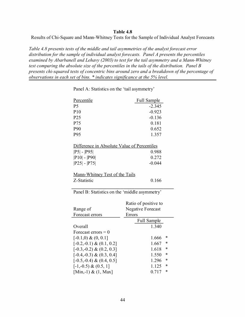
44

Table 4.8Results of Chi-Square and Mann-Whitney Tests for the Sample of Individual Analyst Forecasts

Table 4.8 presents tests of the middle and tail asymmetries of the analyst forecast errordistribution for the sample of individual analyst forecasts. Panel A presents the percentilesexamined by Abarbanell and Lehavy (2003) to test for the tail asymmetry and a Mann-Whitneytest comparing the absolute size of the percentiles in the tails of the distribution. Panel Bpresents chi-squared tests of concentric bins around zero and a breakdown of the percentage ofobservations in each set of bins. * indicates significance at the 5% level.

Panel A: Statistics on the ‘tail asymmetry’

Percentile Full SampleP5 -2.345P10 -0.923P25 -0.136P75 0.181P90 0.652P95 1.357

Difference in Absolute Value of Percentiles |P5| - |P95| 0.988|P10| - |P90| 0.272|P25| - |P75| -0.044

Mann-Whitney Test of the TailsZ-Statistic 0.166 Panel B: Statistics on the ‘middle asymmetry’

Ratio of positive to Range ofForecast errors

Negative ForecastErrors

Full SampleOverall 1.340Forecast errors = 0[-0.1,0) & (0, 0.1] 1.666 *[-0.2,-0.1) & (0.1, 0.2] 1.667 *[-0.3,-0.2) & (0.2, 0.3] 1.618 *[-0.4,-0.3) & (0.3, 0.4] 1.550 *[-0.5,-0.4) & (0.4, 0.5] 1.296 *[-1,-0.5) & (0.5, 1] 1.125 *[Min,-1) & (1, Max] 0.717 *

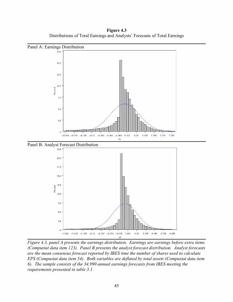
45

Figure 4.3Distributions of Total Earnings and Analysts’ Forecasts of Total Earnings

Panel A: Earnings Distribution

Panel B: Analyst Forecast Distribution

Figure 4.3, panel A presents the earnings distribution. Earnings are earnings before extra items(Compustat data item 123). Panel B presents the analyst forecast distribution. Analyst forecastsare the mean consensus forecast reported by IBES time the number of shares used to calculateEPS (Compustat data item 54). Both variables are deflated by total assets (Compustat data item6). The sample consists of the 34,990 annual earnings forecasts from IBES meeting therequirements presented in table 3.1.

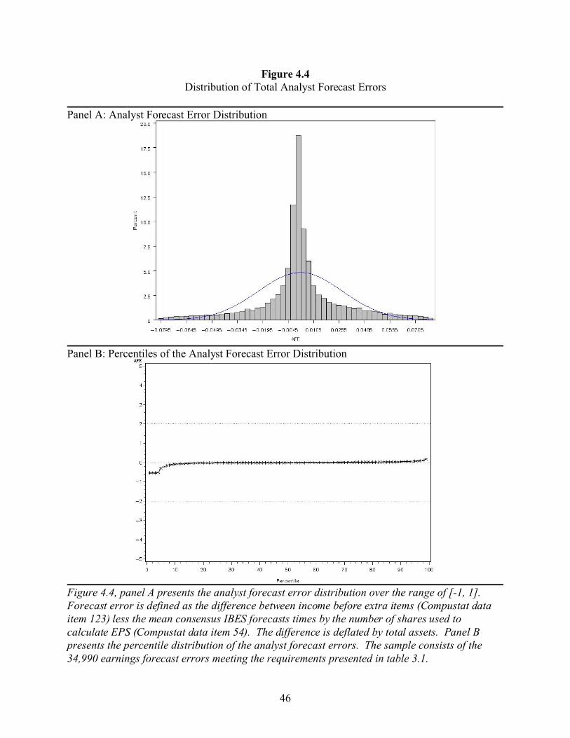
46

Figure 4.4Distribution of Total Analyst Forecast Errors

Panel A: Analyst Forecast Error Distribution

Panel B: Percentiles of the Analyst Forecast Error Distribution

Figure 4.4, panel A presents the analyst forecast error distribution over the range of [-1, 1]. Forecast error is defined as the difference between income before extra items (Compustat dataitem 123) less the mean consensus IBES forecasts times by the number of shares used tocalculate EPS (Compustat data item 54). The difference is deflated by total assets. Panel Bpresents the percentile distribution of the analyst forecast errors. The sample consists of the34,990 earnings forecast errors meeting the requirements presented in table 3.1.

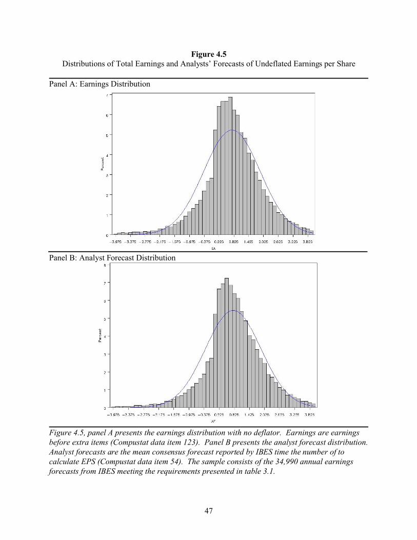
47

Figure 4.5Distributions of Total Earnings and Analysts’ Forecasts of Undeflated Earnings per Share

Panel A: Earnings Distribution

Panel B: Analyst Forecast Distribution

Figure 4.5, panel A presents the earnings distribution with no deflator. Earnings are earningsbefore extra items (Compustat data item 123). Panel B presents the analyst forecast distribution. Analyst forecasts are the mean consensus forecast reported by IBES time the number of tocalculate EPS (Compustat data item 54). The sample consists of the 34,990 annual earningsforecasts from IBES meeting the requirements presented in table 3.1.

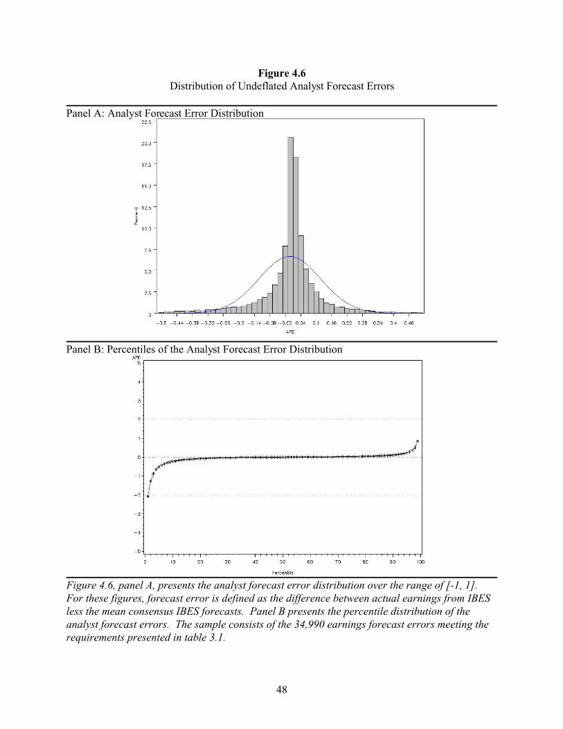
48

Figure 4.6Distribution of Undeflated Analyst Forecast Errors

Panel A: Analyst Forecast Error Distribution

Panel B: Percentiles of the Analyst Forecast Error Distribution

Figure 4.6, panel A, presents the analyst forecast error distribution over the range of [-1, 1]. For these figures, forecast error is defined as the difference between actual earnings from IBESless the mean consensus IBES forecasts. Panel B presents the percentile distribution of theanalyst forecast errors. The sample consists of the 34,990 earnings forecast errors meeting therequirements presented in table 3.1.

49

CHAPTER 5

THE REGRESSION MODEL

5.1 Defining the Model

In order to examine how analysts treat earnings management when making their forecasts,

I use a variation of the model used by Elgers, et al. (2003) to test working capital accruals. The

current model consists of two equations. In the first equation, year ahead earnings are regressed

on current cash flows, nondiscretionary accruals, and discretionary accruals. The estimated

coefficient on each component of current earnings indicates its predictive ability for future

earnings. In the second equation, analysts’ forecasts of year ahead earnings are regressed on

current period earnings components. In this equation, the coefficients on each earnings

component indicate analysts’ weighting of that component in their forecast. I assume that if

analysts aim for forecast accuracy, they will weight the earnings components according to their

predictive ability, and the coefficients for particular components will not differ across equations.

In contrast, differences between coefficients indicate cases where analysts depart from accuracy

as their forecasting goal. Thus, if analysts remove the effects of earnings management, they will

discount discretionary accruals to provide information about current earnings management, even

at the expense of some current information content contained in discretionary accruals.

Formally, the model is written:

EAt+1 = "0 + "1CFOt + "2NDACCt + "3DACCt + gt+1 (1)

AFt+1 = $0 + $1CFOt + $2NDACCt + $3DACCt + <t+1 (2)

7I winsorize EAt+1 at the 1st and 99th percentiles because the mean consensus analystforecast is similarly winsorized (see section 3.1).

50

where EAt+1 is earnings before extra items at time t+1 (Compustat data item 123),7 AFt+1 is the

mean consensus analyst forecast of reported earnings at time t+1 multiplied by the number of

shares used to calculate EPS (IBES data item ‘meanest’ times Compustat data item 54), CFOt is

cash flows from operations as defined by Hribar and Collins (2002), DACCt is discretionary

accruals from the modified-Jones model (discussed in section 5.4), and NDACCt is non-

discretionary accruals, calculated as the difference between CFOt and DACCt. All variables are

deflated by lagged total assets (Compustat data item 6).

This model is similar in form to the simultaneous equation models used by Sloan (1996)

and Xie (2001). In their studies, Sloan and Xie use a system of equations approach to regress

upcoming earnings and stock price on the current earnings components and test whether

investors correctly weight the information content of current earnings. For their tests, the

differences between the dependent variables, earnings and stock price, are sufficient to allow the

models to meet the assumption of independence needed to run a system of simultaneous

equations. The dependent variables in the current model, however, are earnings and analysts

forecasts of earnings. This relationship between these two dependent variables leads to cross-

sectional dependence in the error terms of equations one and two that violates the assumption of

independence and results in biased estimates (Bernard 1987). To avoid this problem, equations

one and two are not run as a system of simultaneous equations but are estimated independently

for each sample year. The mean value for each of the coefficients is then calculated, and cross-

equation differences in coefficients are evaluated using a standard t-test (Elgers et al. 2003).

51

5.2 Assumptions

The testing strategy described in section 5.1 relies on several assumptions. First,

consistent with prior research (such as Bartov, Gul and Tsui 2001, Gaver, Gaver and Austin

1995, Hribar and Collins 2002, Jones 1991, and Kothari, Leone and Wasley 2005), I assume that

discretionary accruals capture the earnings management component of reported earnings.

Second, I assume that analysts communicate their knowledge of earnings management in their

forecast, rather than in other disclosures in the body of their report. This focus on forecasts

rather than recommendations is consistent with Abarbanell and Bernard (2000), Barron, Kim,

Lim and Stevens (1998), Bradshaw, Richardson and Sloan (2001), Crichfield, Dyckman and

Lakonishok (1978), Elgers, Lo and Pfeiffer Jr. (2001), and Schipper (1991). In addition, I

assume that analysts issue only one earnings forecast rather than separately forecasting reported

and premanaged earnings, consistent with the assumptions of Abarbanell and Lehavy (2003),

Burgstahler and Eames (2003), and Liu (2005). Finally, I assume that analysts can separate

discretionary accruals into earnings management and legitimate changes in accruals (Abarbanell

and Lehavy 2003 and Balsam, Bartov and Marquardt 2002).

5.3 Predictions

Based on the findings of Elgers, et al. (2003) and Xie (2001), I predict that the

components of current earnings will be positively related to both upcoming earnings and

analysts’ forecasts of upcoming earnings. This leads to my first hypothesis:

H1: All of the coefficients from equations one and two will be positive.

I assume that analysts understand the implications of cash flows and nondiscretionary accruals

for upcoming earnings. Thus, I predict that the difference between the coefficients from

52

equations one and two on cash flows from operations and nondiscretionary accruals will be zero.

This leads to the second hypothesis:

H2: There will be no difference between the coefficients on either cash flows fromoperations or nondiscretionary accruals in equations one and two.

If analysts include the effects of earnings management in their forecasts, as predicted by

Burgstahler and Eames (2003), there will be no difference between the coefficients on

discretionary accruals in equations one and two. This leads to hypothesis three:

H3: If analysts include the effects of earnings management in their forecasts, thenthere will be no difference between the coefficients on discretionary accruals inequations one and two.

Rejection of hypothesis three indicates that discretionary accruals are weighted differently by

analysts than would be indicated by their predictive ability for future earnings. A finding that the

coefficient on discretionary accruals in equation two is significantly lower than the weight in

equation one is consistent with analysts' discounting earnings management when making their

forecasts. Such a finding would support the view of Abarbanell and Lehavy (2003).

5.4 Calculating Discretionary Accruals

I calculate discretionary accruals using the cross-sectional version of the modified-Jones

model. I estimate the model cross-sectionally for each year, rather than by individual firm over

time, for two reasons. First, Bartov, et al. (2001) show that the cross-section version is more

accurate than the time-series model. Second, the cross-sectional model provides a larger sample

size relative to the time-series models. I estimate the model for each two-digit Standard

Industrial Code (SIC) and year combination with at least five observations, consistent with Xie

(2001). In addition, I include return on assets to control for legitimate changes in accruals due to

performance (Kothari et al. 2005). The model is:

53

TAt = b1(1/At-1) + b2)REVt + b3PPEt + b4ROAt + et (3)

where, TAt is total accruals for year t calculated as the difference between earnings before extra

items (Compustat annual data item 123) and cash flows from operations (Compustat annual data

item 308 less Compustat annual data item 124), At-1 is lagged total assets (Compustat annual data

item 6), )REVt is the change in sales less the change in accounts receivable (Compustat annual

data items 12 and 2, respectively), PPEt is gross property plant and equipment (Compustat annual

data item 8), and ROAt is return on assets (Compustat annual data item 172 divided by lagged

total assets). TAt, )REVt, and PPEt are deflated by lagged total assets. Discretionary accruals

(DACCt) are the residuals from equation three.

5.5 Summary Statistics

Table 5.1 presents the summary statistics for the variables used in equations one and two.

Consistent with Burgstahler and Eames (2003), I find that the mean year-ahead analyst forecast

(0.016) and actual year-ahead earnings (0.017) are similar (p-value = 0.9831). However, the

year-ahead forecast (AFt+1) is much more variable than year-ahead earnings, as shown by both the

larger standard deviation and the more extreme minimum and maximum values. This is because

AFt+1 is formed by multiplying the mean consensus forecast by the number of shares used to

calculate EPS. This exposes AFt+1 to the variation of both variables. The alternative winsorizing

method presented in section 5.7.3 attempts to address this issue.

Cash flows from operations are significantly positive, while the mean values for both

nondiscretionary and discretionary accruals are significantly negative. Discretionary accruals are

significantly smaller in magnitude (p < 0.001) and appear less variable than nondiscretionary

accruals. Also, the high positive values for both the 75th percentile and the maximum suggest

54

that discretionary accruals are used, at least in some cases, to increase total earnings, suggesting

that they are used to manage earnings. These results are consistent with those of prior research

(see, for example, Elgers et al. 2003, Sloan 1996, and Xie 2001).

5.6 Results

Table 5.2, panel A, presents the results of estimating equation one, in which upcoming

earnings are regressed on current earnings components. Consistent with hypothesis one, the

coefficients are positive on all three variables. I test for significance using both a traditional t-

test as well as a binomial test (p = 0.5) of the number of positive coefficients among the 16

sample years. Both tests indicate that each component of current earnings is significantly

positively associated with upcoming earnings. Panel B presents the results for equation two, in

which analysts’ forecasts of upcoming earnings are regressed on current earnings components.

Although the binomial test suggests that each variable is significantly positive, the t-tests indicate

that none of the coefficients on the current earning components are significantly different from

zero. This last result is contrary to hypothesis one.

Panel C reports the differences in the average coefficient values reported in panels A and

B. The coefficients on discretionary accruals ($3 and "3) do not differ significantly between

equations, consistent with hypothesis three. Likewise, the cross-equation differences between the

coefficients on cash flows from operations and nondiscretionary accruals are insignificant,

consistent with hypothesis two. It cannot be concluded, however that analysts correctly weight

the information from all three earnings components when forecasting upcoming earnings,

because the insignificant coefficients in panel B suggest that they do not use the earnings

information in forming their forecasts.

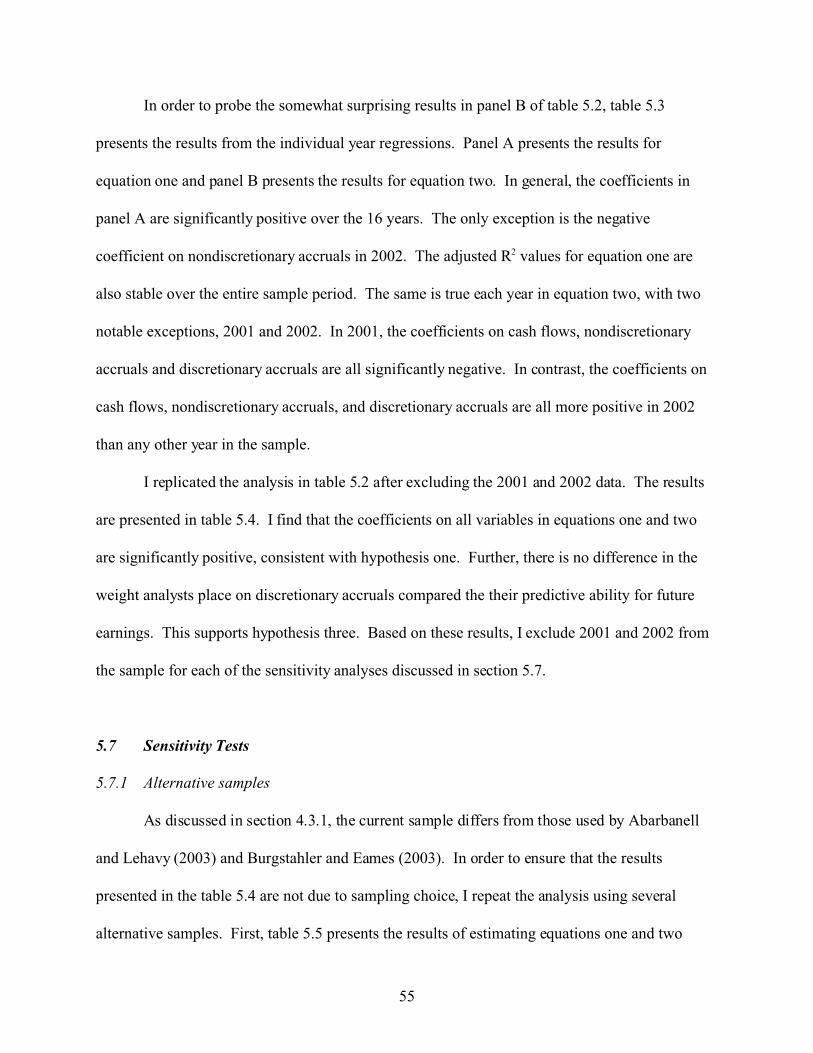
55

In order to probe the somewhat surprising results in panel B of table 5.2, table 5.3

presents the results from the individual year regressions. Panel A presents the results for

equation one and panel B presents the results for equation two. In general, the coefficients in

panel A are significantly positive over the 16 years. The only exception is the negative

coefficient on nondiscretionary accruals in 2002. The adjusted R2 values for equation one are

also stable over the entire sample period. The same is true each year in equation two, with two

notable exceptions, 2001 and 2002. In 2001, the coefficients on cash flows, nondiscretionary

accruals and discretionary accruals are all significantly negative. In contrast, the coefficients on

cash flows, nondiscretionary accruals, and discretionary accruals are all more positive in 2002

than any other year in the sample.

I replicated the analysis in table 5.2 after excluding the 2001 and 2002 data. The results

are presented in table 5.4. I find that the coefficients on all variables in equations one and two

are significantly positive, consistent with hypothesis one. Further, there is no difference in the

weight analysts place on discretionary accruals compared the their predictive ability for future

earnings. This supports hypothesis three. Based on these results, I exclude 2001 and 2002 from

the sample for each of the sensitivity analyses discussed in section 5.7.

5.7 Sensitivity Tests

5.7.1 Alternative samples

As discussed in section 4.3.1, the current sample differs from those used by Abarbanell

and Lehavy (2003) and Burgstahler and Eames (2003). In order to ensure that the results

presented in the table 5.4 are not due to sampling choice, I repeat the analysis using several

alternative samples. First, table 5.5 presents the results of estimating equations one and two

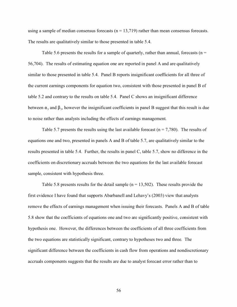
56

using a sample of median consensus forecasts (n = 13,719) rather than mean consensus forecasts.

The results are qualitatively similar to those presented in table 5.4.

Table 5.6 presents the results for a sample of quarterly, rather than annual, forecasts (n =

56,704). The results of estimating equation one are reported in panel A and are qualitatively

similar to those presented in table 5.4. Panel B reports insignificant coefficients for all three of

the current earnings components for equation two, consistent with those presented in panel B of

table 5.2 and contrary to the results on table 5.4. Panel C shows an insignificant difference

between "3 and $3, however the insignificant coefficients in panel B suggest that this result is due

to noise rather than analysts including the effects of earnings management.

Table 5.7 presents the results using the last available forecast (n = 7,780). The results of

equations one and two, presented in panels A and B of table 5.7, are qualitatively similar to the

results presented in table 5.4. Further, the results in panel C, table 5.7, show no difference in the

coefficients on discretionary accruals between the two equations for the last available forecast

sample, consistent with hypothesis three.

Table 5.8 presents results for the detail sample (n = 13,502). These results provide the

first evidence I have found that supports Abarbanell and Lehavy’s (2003) view that analysts

remove the effects of earnings management when issuing their forecasts. Panels A and B of table

5.8 show that the coefficients of equations one and two are significantly positive, consistent with

hypothesis one. However, the differences between the coefficients of all three coefficients from

the two equations are statistically significant, contrary to hypotheses two and three. The

significant difference between the coefficients in cash flow from operations and nondiscretionary

accruals components suggests that the results are due to analyst forecast error rather than to

57

analysts intentionally removing earnings management (see, for example, Bradshaw, et al. 2001

and Elgers, et al. 2003).

5.7.2 Firms likely to manage earnings.

The current sample makes no attempt to distinguish among firms according to their

likelihood of managing earnings. For firms that do not manage earnings, $3 will equal "3

because there is no earnings management to be removed. These firms cannot be used to decide

whether analysts include or remove earnings management from their forecasts. To address this

issue, I estimate equations one and two using a sub-sample of firms that I consider to be likely to

engage in earnings management. The sample consists of those firms with deflated earnings per

share in the range [-0.01, 0.01]. This restriction is based on evidence (see, for example, Ayers,

Jiang and Yeung 2006, Burgstahler and Dichev 1997, DeFond and Park 1997, and Matsumoto

2002) that firms immediately around the zero benchmark have incentives to manage earnings,

with those firms managing to meet-or-beat the benchmark being successful in their efforts.

The results are shown in tables 5.9. Consistent with hypothesis one, the coefficients from

both equations are significantly positive. However, the differences between the coefficients of

all three coefficients from the two equations are significant, contrary to hypotheses two and three.

While the significant difference on the discretionary accruals variable suggests that analysts

remove the effects of earnings management for firms likely to manage earnings, the significant

difference on the other earnings components suggests that the difference is due to analyst forecast

error rather than to analysts intentionally removing earnings management from their forecasts.

58

5.7.3 Winsorizing

Abarbanell and Lehavy (2003) control for outliers by winsorizing earnings per share and

analyst forecasts at the 1st and 99th percentiles. Similarly, Elgers et al. (2003) truncate their

measure of earnings and analyst forecasts at the 1st and 99th percentiles. Burgstahler and Eames

(2003), on the other hand, do not winsorize or truncate their sample. For the principal tests, I

winsorized analysts forecasts (IBES data item ‘meanest’) and year-ahead earnings (Compustat

data item 123) at the 1st and 99th percentiles. I replicated my tests without winsorizing for

consistency with Burgstahler and Eames (2003). The results, presented in table 5.10, show no

evidence of a difference in the coefficients on discretionary accruals from the two regressions.

However, since the coefficients on cash flow from operations and discretionary accruals reported

on panel B are insignificant, this result is likely due to the increase in variance caused by the lack

of winsorizing.

I also estimated equations one and two using a different winsorizing strategy compared to

my original analysis in order to control for the high variability in AFt+1 relative to year-ahead

earnings documented in table 5.1. Specifically, I created the AFt+1 variable by multiplying the

mean consensus forecast, already winsorized, by the number of shares used to calculate EPS

(Compustat data item 54) and then winsorized at the 1st and 99th percentiles. The results are

presented in table 5.11. Panels A and B show that the coefficients on the three current earnings

components are positively statistically significant for both equations, consistent with hypothesis

one and the results in table 5.4. The t-tests presented in panel C indicate that both cash flows

from operations and discretionary accruals are discounted by analysts. The significant difference

on discretionary accruals is consistent with Abarbanell and Lehavy’s (2003) prediction that

analysts remove the effects of earnings management. The significant difference between the

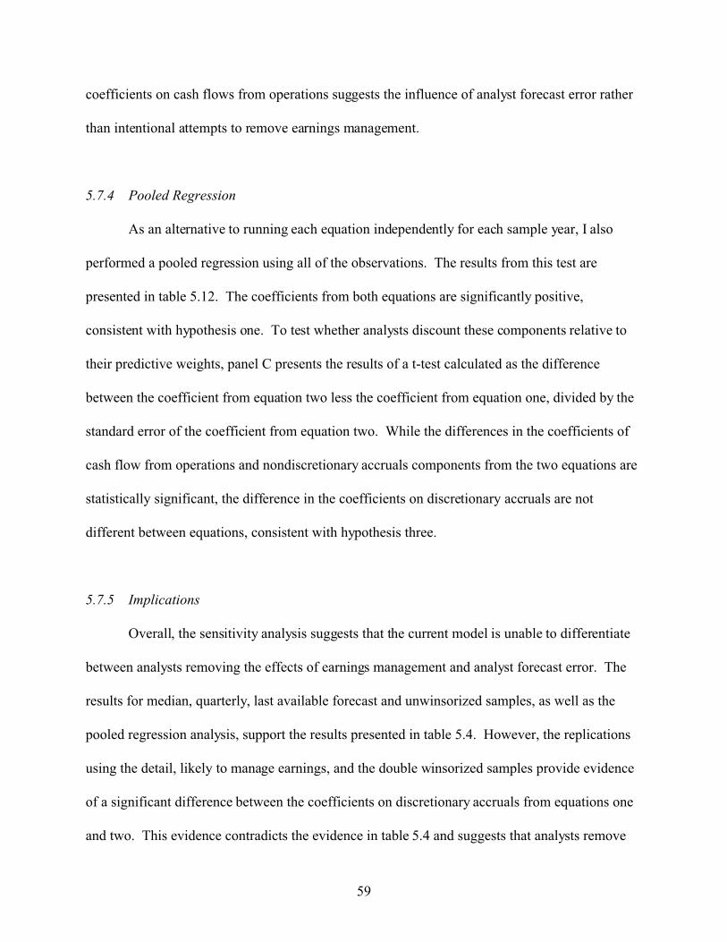
59

coefficients on cash flows from operations suggests the influence of analyst forecast error rather

than intentional attempts to remove earnings management.

5.7.4 Pooled Regression

As an alternative to running each equation independently for each sample year, I also

performed a pooled regression using all of the observations. The results from this test are

presented in table 5.12. The coefficients from both equations are significantly positive,

consistent with hypothesis one. To test whether analysts discount these components relative to

their predictive weights, panel C presents the results of a t-test calculated as the difference

between the coefficient from equation two less the coefficient from equation one, divided by the

standard error of the coefficient from equation two. While the differences in the coefficients of

cash flow from operations and nondiscretionary accruals components from the two equations are

statistically significant, the difference in the coefficients on discretionary accruals are not

different between equations, consistent with hypothesis three.

5.7.5 Implications

Overall, the sensitivity analysis suggests that the current model is unable to differentiate

between analysts removing the effects of earnings management and analyst forecast error. The

results for median, quarterly, last available forecast and unwinsorized samples, as well as the

pooled regression analysis, support the results presented in table 5.4. However, the replications

using the detail, likely to manage earnings, and the double winsorized samples provide evidence

of a significant difference between the coefficients on discretionary accruals from equations one

and two. This evidence contradicts the evidence in table 5.4 and suggests that analysts remove

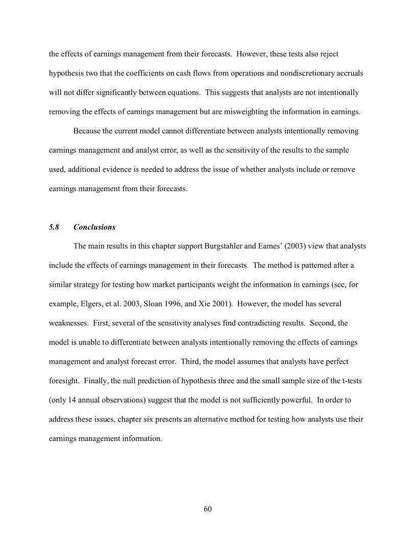
60

the effects of earnings management from their forecasts. However, these tests also reject

hypothesis two that the coefficients on cash flows from operations and nondiscretionary accruals

will not differ significantly between equations. This suggests that analysts are not intentionally

removing the effects of earnings management but are misweighting the information in earnings.

Because the current model cannot differentiate between analysts intentionally removing

earnings management and analyst error, as well as the sensitivity of the results to the sample

used, additional evidence is needed to address the issue of whether analysts include or remove

earnings management from their forecasts.

5.8 Conclusions

The main results in this chapter support Burgstahler and Eames’ (2003) view that analysts

include the effects of earnings management in their forecasts. The method is patterned after a

similar strategy for testing how market participants weight the information in earnings (see, for

example, Elgers, et al. 2003, Sloan 1996, and Xie 2001). However, the model has several

weaknesses. First, several of the sensitivity analyses find contradicting results. Second, the

model is unable to differentiate between analysts intentionally removing the effects of earnings

management and analyst forecast error. Third, the model assumes that analysts have perfect

foresight. Finally, the null prediction of hypothesis three and the small sample size of the t-tests

(only 14 annual observations) suggest that the model is not sufficiently powerful. In order to

address these issues, chapter six presents an alternative method for testing how analysts use their

earnings management information.

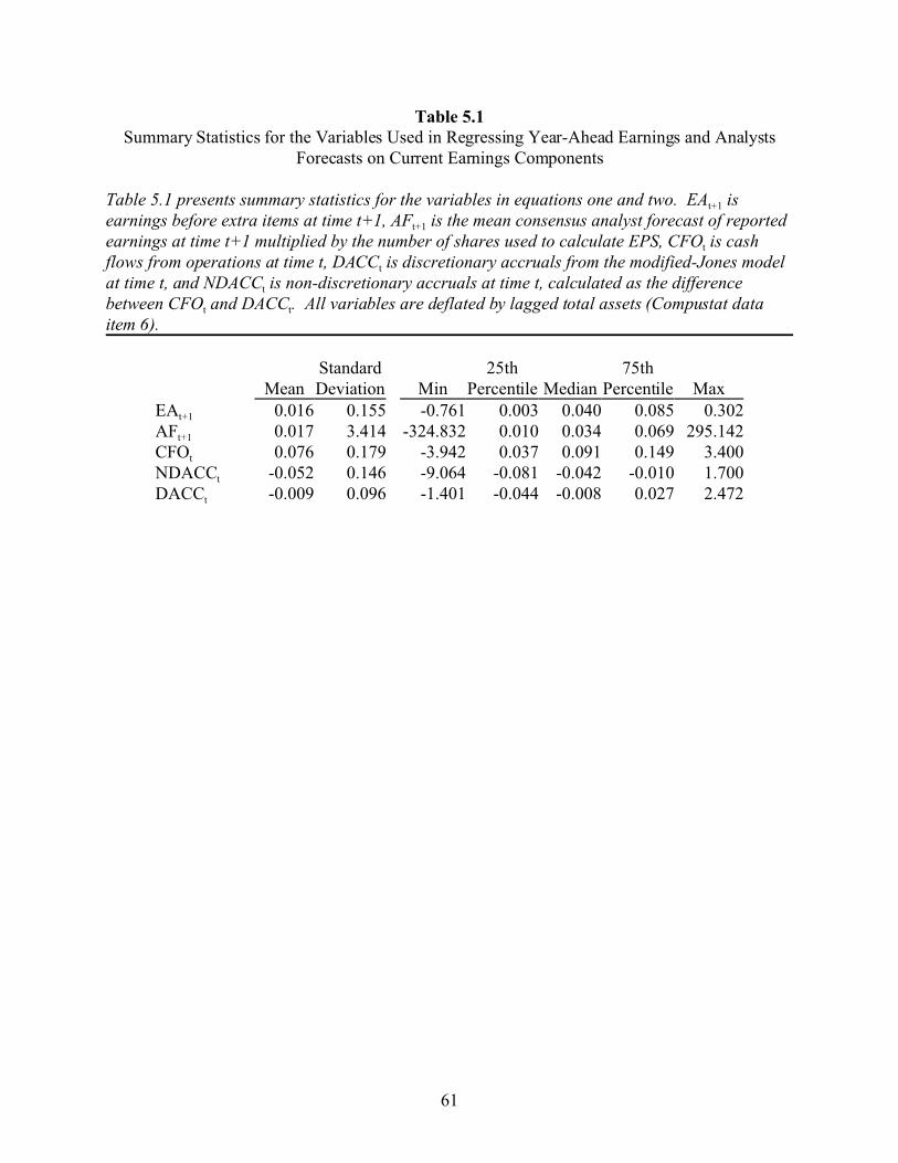
61

Table 5.1Summary Statistics for the Variables Used in Regressing Year-Ahead Earnings and Analysts

Forecasts on Current Earnings Components

Table 5.1 presents summary statistics for the variables in equations one and two. EAt+1 isearnings before extra items at time t+1, AFt+1 is the mean consensus analyst forecast of reportedearnings at time t+1 multiplied by the number of shares used to calculate EPS, CFOt is cashflows from operations at time t, DACCt is discretionary accruals from the modified-Jones modelat time t, and NDACCt is non-discretionary accruals at time t, calculated as the differencebetween CFOt and DACCt. All variables are deflated by lagged total assets (Compustat dataitem 6).

Standard 25th 75thMean Deviation Min Percentile Median Percentile Max

EAt+1 0.016 0.155 -0.761 0.003 0.040 0.085 0.302AFt+1 0.017 3.414 -324.832 0.010 0.034 0.069 295.142CFOt 0.076 0.179 -3.942 0.037 0.091 0.149 3.400NDACCt -0.052 0.146 -9.064 -0.081 -0.042 -0.010 1.700DACCt -0.009 0.096 -1.401 -0.044 -0.008 0.027 2.472

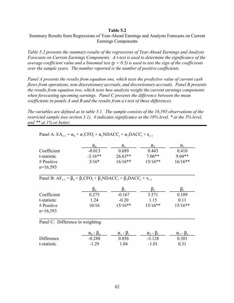
62

Table 5.2Summary Results from Regressions of Year-Ahead Earnings and Analysts Forecasts on Current

Earnings Components

Table 5.2 presents the summary results of the regressions of Year-Ahead Earnings and AnalystsForecasts on Current Earnings Components. A t-test is used to determine the significance of theaverage coefficient value and a binomial test (p = 0.5) is used to test the sign of the coefficientsover the sample years. The number reported is the number of positive coefficients.

Panel A presents the results from equation one, which tests the predictive value of current cashflows from operations, non-discretionary accruals, and discretionary accruals. Panel B presentsthe results from equation two, which tests how analysts weight the current earnings componentswhen forecasting upcoming earnings. Panel C presents the difference between the meancoefficients in panels A and B and the results from a t-test of these differences.

The variables are defined as in table 5.1. The sample consists of the 16,593 observations of therestricted sample (see section 3.1). # indicates significance at the 10% level, * at the 5% level,and ** at 1% or better.

Panel A: EAt+1 = "0 + "1CFOt + "2NDACCt + "3DACCt + gt+1

"0 "1 "2 "3

Coefficient -0.013 0.689 0.443 0.410t-statistic -3.16** 26.63** 7.06** 9.04**# Positive 3/16* 16/16** 15/16** 16/16**n=16,593 Panel B: AFt+1 = $0 + $1CFOt + $2NDACCt + $3DACCt + <t+1

$0 $1 $2 $3

Coefficient 0.275 -0.167 3.571 0.109t-statistic 1.24 -0.20 1.15 0.11# Positive 10/16 15/16** 15/16** 15/16**n=16,593 Panel C: Difference in weighting

"0 - $0 "1 - $1 "2 - $2 "3 - $3

Difference -0.288 0.856 -3.128 0.301t-statistic -1.29 1.04 -1.01 0.31

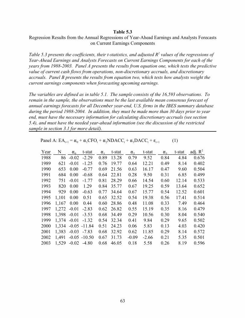
63

Table 5.3Regression Results from the Annual Regressions of Year-Ahead Earnings and Analysts Forecasts

on Current Earnings Components

Table 5.3 presents the coefficients, their t-statistics, and adjusted R2 values of the regressions ofYear-Ahead Earnings and Analysts Forecasts on Current Earnings Components for each of theyears from 1988-2003. Panel A presents the results from equation one, which tests the predictivevalue of current cash flows from operations, non-discretionary accruals, and discretionaryaccruals. Panel B presents the results from equation two, which tests how analysts weight thecurrent earnings components when forecasting upcoming earnings.

The variables are defined as in table 5.1. The sample consists of the 16,593 observations. Toremain in the sample, the observations must be the last available mean consensus forecast ofannual earnings forecasts for all December year-end, U.S. firms in the IBES summary databaseduring the period 1988-2004. In addition, they must be made more than 30 days prior to yearend, must have the necessary information for calculating discretionary accruals (see section5.4), and must have the needed year-ahead information (see the discussion of the restrictedsample in section 3.1 for more detail).

Panel A: EAt+1 = "0 + "1CFOt + "2NDACCt + "3DACCt + gt+1 (1)

Year N "0 t-stat "1 t-stat "2 t-stat "3 t-stat adj. R2

1988 86 -0.02 -2.29 0.89 13.28 0.79 9.52 0.84 4.84 0.6761989 621 -0.01 -1.25 0.76 19.77 0.64 12.21 0.49 8.14 0.4021990 653 0.00 -0.77 0.69 21.56 0.63 16.17 0.47 9.60 0.5041991 684 0.00 -0.68 0.64 22.81 0.28 9.50 0.31 6.85 0.4991992 751 -0.01 -1.77 0.81 28.29 0.66 14.54 0.60 12.14 0.5331993 820 0.00 1.29 0.84 35.77 0.67 19.25 0.59 13.64 0.6521994 929 0.00 -0.63 0.77 34.64 0.67 15.77 0.54 12.52 0.6011995 1,101 0.00 0.51 0.65 32.52 0.54 19.38 0.56 17.41 0.5141996 1,167 0.00 0.44 0.60 28.86 0.48 11.08 0.33 7.49 0.4641997 1,272 -0.01 -2.83 0.62 26.82 0.55 15.19 0.35 8.16 0.4791998 1,398 -0.01 -3.53 0.68 34.49 0.29 10.56 0.30 8.04 0.5401999 1,374 -0.01 -1.32 0.54 32.34 0.41 9.84 0.29 9.65 0.5022000 1,334 -0.05 -11.84 0.51 24.23 0.06 5.83 0.13 4.03 0.4202001 1,383 -0.03 -7.83 0.68 32.92 0.62 11.85 0.29 8.14 0.5722002 1,491 -0.05 -10.50 0.67 31.73 -0.09 -2.66 0.21 5.35 0.5012003 1,529 -0.02 -4.80 0.68 46.05 0.18 5.58 0.26 8.19 0.596

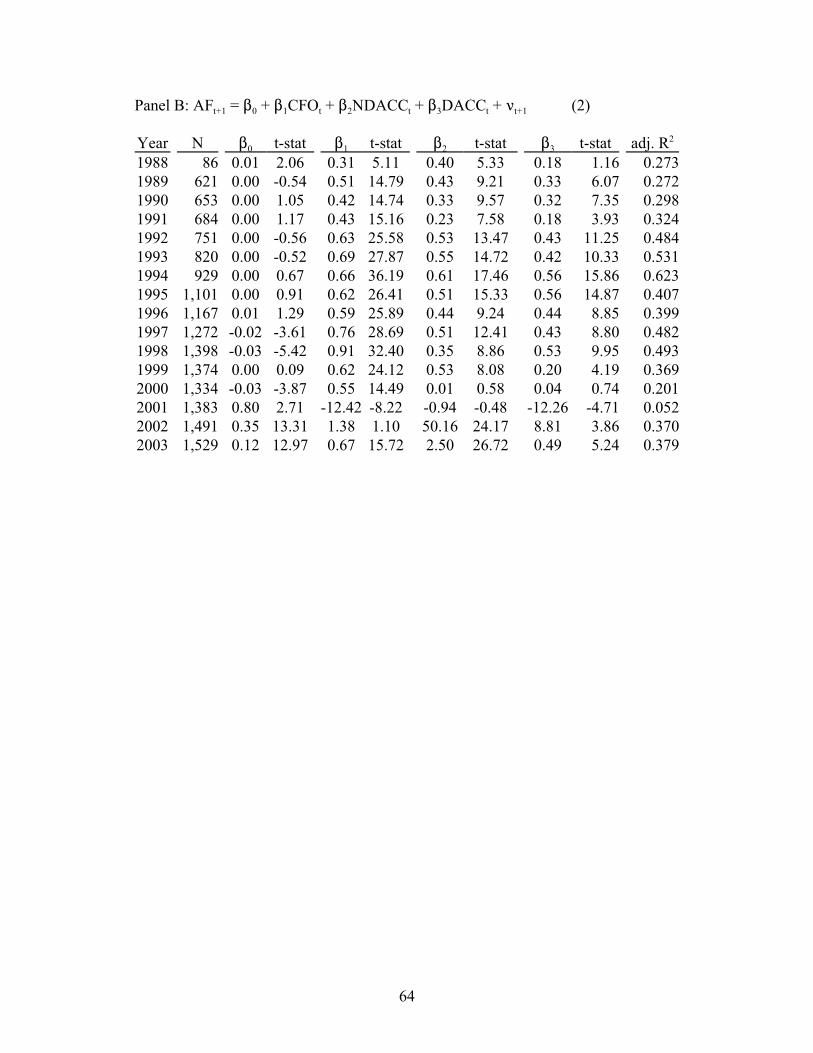
64

Panel B: AFt+1 = $0 + $1CFOt + $2NDACCt + $3DACCt + <t+1 (2)

Year N $0 t-stat $1 t-stat $2 t-stat $3 t-stat adj. R2

1988 86 0.01 2.06 0.31 5.11 0.40 5.33 0.18 1.16 0.2731989 621 0.00 -0.54 0.51 14.79 0.43 9.21 0.33 6.07 0.2721990 653 0.00 1.05 0.42 14.74 0.33 9.57 0.32 7.35 0.2981991 684 0.00 1.17 0.43 15.16 0.23 7.58 0.18 3.93 0.3241992 751 0.00 -0.56 0.63 25.58 0.53 13.47 0.43 11.25 0.4841993 820 0.00 -0.52 0.69 27.87 0.55 14.72 0.42 10.33 0.5311994 929 0.00 0.67 0.66 36.19 0.61 17.46 0.56 15.86 0.6231995 1,101 0.00 0.91 0.62 26.41 0.51 15.33 0.56 14.87 0.4071996 1,167 0.01 1.29 0.59 25.89 0.44 9.24 0.44 8.85 0.3991997 1,272 -0.02 -3.61 0.76 28.69 0.51 12.41 0.43 8.80 0.4821998 1,398 -0.03 -5.42 0.91 32.40 0.35 8.86 0.53 9.95 0.4931999 1,374 0.00 0.09 0.62 24.12 0.53 8.08 0.20 4.19 0.3692000 1,334 -0.03 -3.87 0.55 14.49 0.01 0.58 0.04 0.74 0.2012001 1,383 0.80 2.71 -12.42 -8.22 -0.94 -0.48 -12.26 -4.71 0.0522002 1,491 0.35 13.31 1.38 1.10 50.16 24.17 8.81 3.86 0.3702003 1,529 0.12 12.97 0.67 15.72 2.50 26.72 0.49 5.24 0.379

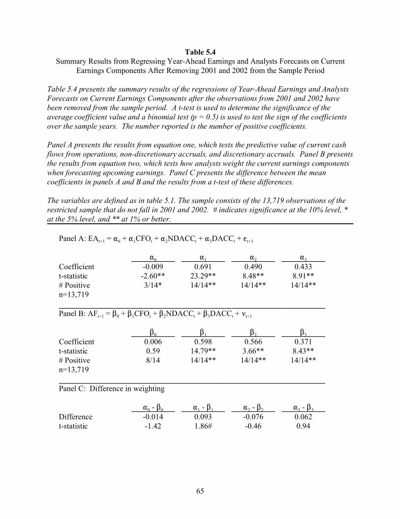
65

Table 5.4Summary Results from Regressing Year-Ahead Earnings and Analysts Forecasts on Current

Earnings Components After Removing 2001 and 2002 from the Sample Period

Table 5.4 presents the summary results of the regressions of Year-Ahead Earnings and AnalystsForecasts on Current Earnings Components after the observations from 2001 and 2002 havebeen removed from the sample period. A t-test is used to determine the significance of theaverage coefficient value and a binomial test (p = 0.5) is used to test the sign of the coefficientsover the sample years. The number reported is the number of positive coefficients.

Panel A presents the results from equation one, which tests the predictive value of current cashflows from operations, non-discretionary accruals, and discretionary accruals. Panel B presentsthe results from equation two, which tests how analysts weight the current earnings componentswhen forecasting upcoming earnings. Panel C presents the difference between the meancoefficients in panels A and B and the results from a t-test of these differences.

The variables are defined as in table 5.1. The sample consists of the 13,719 observations of therestricted sample that do not fall in 2001 and 2002. # indicates significance at the 10% level, *at the 5% level, and ** at 1% or better.

Panel A: EAt+1 = "0 + "1CFOt + "2NDACCt + "3DACCt + gt+1

"0 "1 "2 "3

Coefficient -0.009 0.691 0.490 0.433t-statistic -2.60** 23.29** 8.48** 8.91**# Positive 3/14* 14/14** 14/14** 14/14**n=13,719 Panel B: AFt+1 = $0 + $1CFOt + $2NDACCt + $3DACCt + <t+1

$0 $1 $2 $3

Coefficient 0.006 0.598 0.566 0.371t-statistic 0.59 14.79** 3.66** 8.43**# Positive 8/14 14/14** 14/14** 14/14**n=13,719 Panel C: Difference in weighting

"0 - $0 "1 - $1 "2 - $2 "3 - $3

Difference -0.014 0.093 -0.076 0.062t-statistic -1.42 1.86# -0.46 0.94

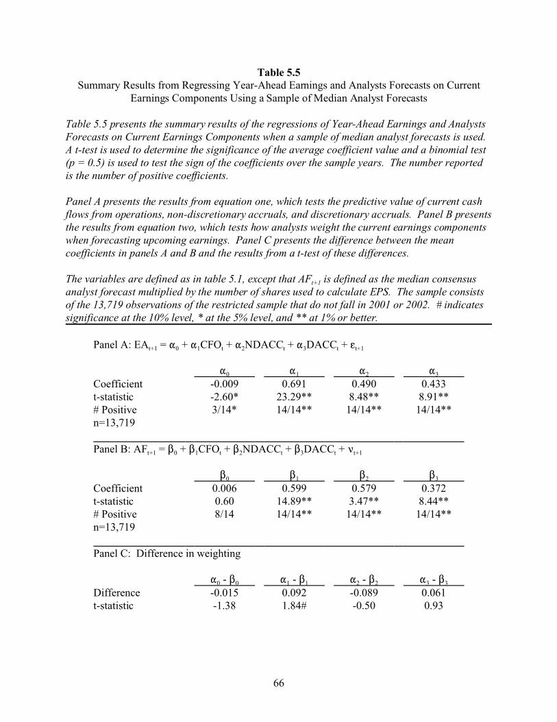
66

Table 5.5Summary Results from Regressing Year-Ahead Earnings and Analysts Forecasts on Current

Earnings Components Using a Sample of Median Analyst Forecasts

Table 5.5 presents the summary results of the regressions of Year-Ahead Earnings and AnalystsForecasts on Current Earnings Components when a sample of median analyst forecasts is used. A t-test is used to determine the significance of the average coefficient value and a binomial test(p = 0.5) is used to test the sign of the coefficients over the sample years. The number reportedis the number of positive coefficients.

Panel A presents the results from equation one, which tests the predictive value of current cashflows from operations, non-discretionary accruals, and discretionary accruals. Panel B presentsthe results from equation two, which tests how analysts weight the current earnings componentswhen forecasting upcoming earnings. Panel C presents the difference between the meancoefficients in panels A and B and the results from a t-test of these differences.

The variables are defined as in table 5.1, except that AFt+1 is defined as the median consensusanalyst forecast multiplied by the number of shares used to calculate EPS. The sample consistsof the 13,719 observations of the restricted sample that do not fall in 2001 or 2002. # indicatessignificance at the 10% level, * at the 5% level, and ** at 1% or better.

Panel A: EAt+1 = "0 + "1CFOt + "2NDACCt + "3DACCt + gt+1

"0 "1 "2 "3

Coefficient -0.009 0.691 0.490 0.433t-statistic -2.60* 23.29** 8.48** 8.91**# Positive 3/14* 14/14** 14/14** 14/14**n=13,719 Panel B: AFt+1 = $0 + $1CFOt + $2NDACCt + $3DACCt + <t+1

$0 $1 $2 $3

Coefficient 0.006 0.599 0.579 0.372t-statistic 0.60 14.89** 3.47** 8.44**# Positive 8/14 14/14** 14/14** 14/14**n=13,719 Panel C: Difference in weighting

"0 - $0 "1 - $1 "2 - $2 "3 - $3

Difference -0.015 0.092 -0.089 0.061t-statistic -1.38 1.84# -0.50 0.93

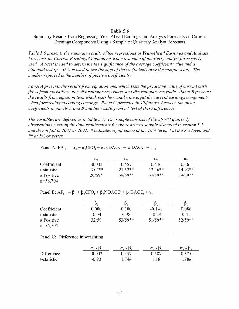
67

Table 5.6Summary Results from Regressing Year-Ahead Earnings and Analysts Forecasts on Current

Earnings Components Using a Sample of Quarterly Analyst Forecasts

Table 5.6 presents the summary results of the regressions of Year-Ahead Earnings and AnalystsForecasts on Current Earnings Components when a sample of quarterly analyst forecasts isused. A t-test is used to determine the significance of the average coefficient value and abinomial test (p = 0.5) is used to test the sign of the coefficients over the sample years. Thenumber reported is the number of positive coefficients.

Panel A presents the results from equation one, which tests the predictive value of current cashflows from operations, non-discretionary accruals, and discretionary accruals. Panel B presentsthe results from equation two, which tests how analysts weight the current earnings componentswhen forecasting upcoming earnings. Panel C presents the difference between the meancoefficients in panels A and B and the results from a t-test of these differences.

The variables are defined as in table 5.1. The sample consists of the 56,704 quarterlyobservations meeting the data requirements for the restricted sample discussed in section 3.1and do not fall in 2001 or 2002. # indicates significance at the 10% level, * at the 5% level, and** at 1% or better.

Panel A: EAt+1 = "0 + "1CFOt + "2NDACCt + "3DACCt + gt+1

"0 "1 "2 "3

Coefficient -0.002 0.557 0.446 0.461t-statistic -3.07** 21.52** 13.36** 14.93**# Positive 20/59* 59/59** 57/59** 59/59**n=56,704 Panel B: AFt+1 = $0 + $1CFOt + $2NDACCt + $3DACCt + <t+1

$0 $1 $2 $3

Coefficient 0.000 0.200 -0.141 0.086t-statistic -0.04 0.98 -0.29 0.41# Positive 32/59 53/59** 51/59** 52/59**n=56,704 Panel C: Difference in weighting

"0 - $0 "1 - $1 "2 - $2 "3 - $3

Difference -0.002 0.357 0.587 0.375t-statistic -0.93 1.74# 1.18 1.78#

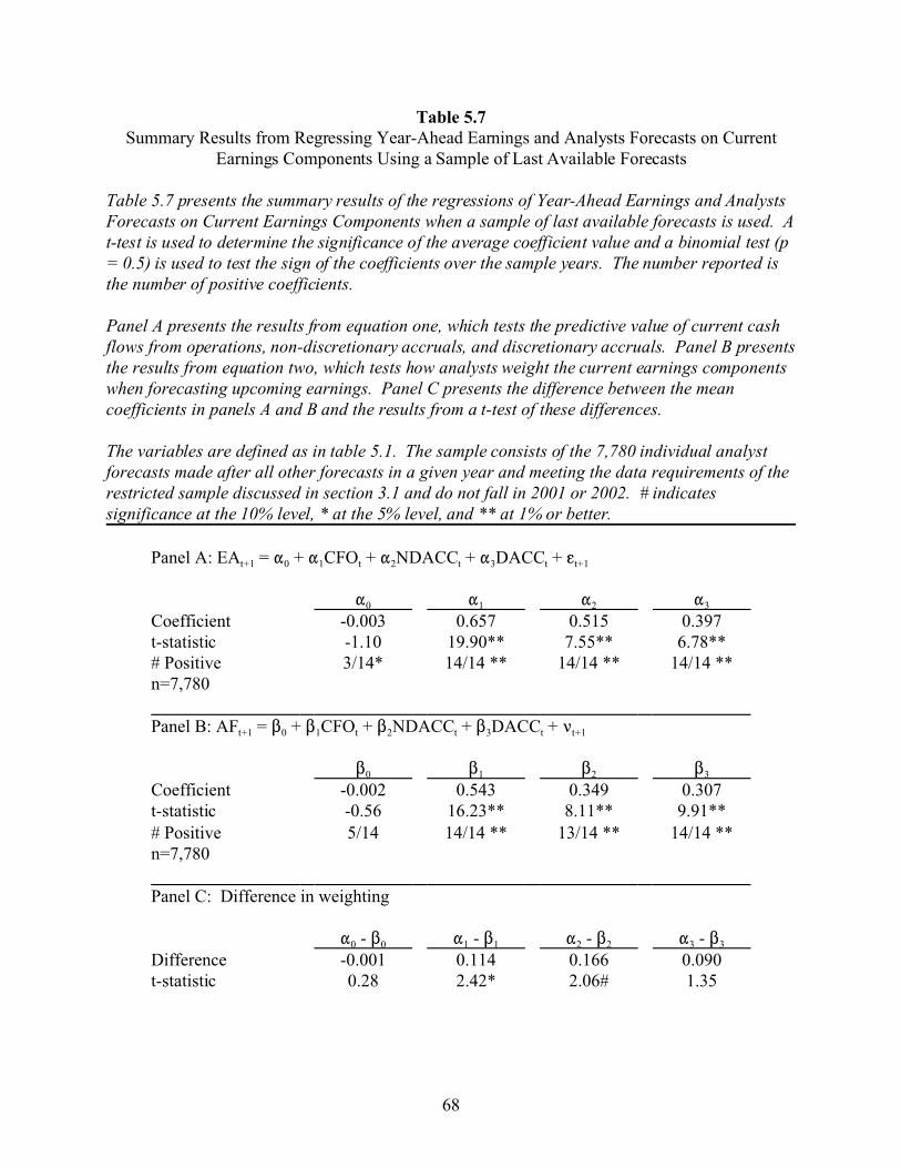
68

Table 5.7Summary Results from Regressing Year-Ahead Earnings and Analysts Forecasts on Current

Earnings Components Using a Sample of Last Available Forecasts

Table 5.7 presents the summary results of the regressions of Year-Ahead Earnings and AnalystsForecasts on Current Earnings Components when a sample of last available forecasts is used. At-test is used to determine the significance of the average coefficient value and a binomial test (p= 0.5) is used to test the sign of the coefficients over the sample years. The number reported isthe number of positive coefficients.

Panel A presents the results from equation one, which tests the predictive value of current cashflows from operations, non-discretionary accruals, and discretionary accruals. Panel B presentsthe results from equation two, which tests how analysts weight the current earnings componentswhen forecasting upcoming earnings. Panel C presents the difference between the meancoefficients in panels A and B and the results from a t-test of these differences.

The variables are defined as in table 5.1. The sample consists of the 7,780 individual analystforecasts made after all other forecasts in a given year and meeting the data requirements of therestricted sample discussed in section 3.1 and do not fall in 2001 or 2002. # indicatessignificance at the 10% level, * at the 5% level, and ** at 1% or better.

Panel A: EAt+1 = "0 + "1CFOt + "2NDACCt + "3DACCt + gt+1

"0 "1 "2 "3

Coefficient -0.003 0.657 0.515 0.397t-statistic -1.10 19.90** 7.55** 6.78**# Positive 3/14* 14/14 ** 14/14 ** 14/14 **n=7,780 Panel B: AFt+1 = $0 + $1CFOt + $2NDACCt + $3DACCt + <t+1

$0 $1 $2 $3

Coefficient -0.002 0.543 0.349 0.307t-statistic -0.56 16.23** 8.11** 9.91**# Positive 5/14 14/14 ** 13/14 ** 14/14 **n=7,780 Panel C: Difference in weighting

"0 - $0 "1 - $1 "2 - $2 "3 - $3

Difference -0.001 0.114 0.166 0.090t-statistic 0.28 2.42* 2.06# 1.35

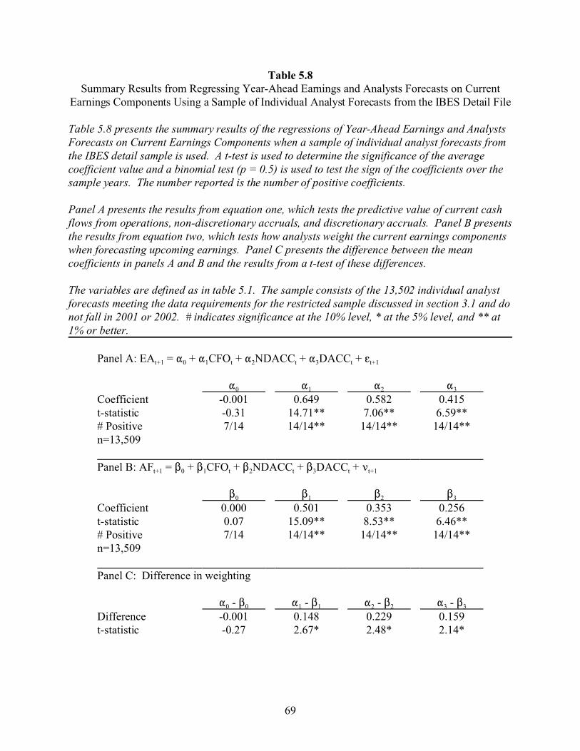
69

Table 5.8Summary Results from Regressing Year-Ahead Earnings and Analysts Forecasts on Current

Earnings Components Using a Sample of Individual Analyst Forecasts from the IBES Detail File

Table 5.8 presents the summary results of the regressions of Year-Ahead Earnings and AnalystsForecasts on Current Earnings Components when a sample of individual analyst forecasts fromthe IBES detail sample is used. A t-test is used to determine the significance of the averagecoefficient value and a binomial test (p = 0.5) is used to test the sign of the coefficients over thesample years. The number reported is the number of positive coefficients.

Panel A presents the results from equation one, which tests the predictive value of current cashflows from operations, non-discretionary accruals, and discretionary accruals. Panel B presentsthe results from equation two, which tests how analysts weight the current earnings componentswhen forecasting upcoming earnings. Panel C presents the difference between the meancoefficients in panels A and B and the results from a t-test of these differences.

The variables are defined as in table 5.1. The sample consists of the 13,502 individual analystforecasts meeting the data requirements for the restricted sample discussed in section 3.1 and donot fall in 2001 or 2002. # indicates significance at the 10% level, * at the 5% level, and ** at1% or better.

Panel A: EAt+1 = "0 + "1CFOt + "2NDACCt + "3DACCt + gt+1

"0 "1 "2 "3

Coefficient -0.001 0.649 0.582 0.415t-statistic -0.31 14.71** 7.06** 6.59**# Positive 7/14 14/14** 14/14** 14/14**n=13,509 Panel B: AFt+1 = $0 + $1CFOt + $2NDACCt + $3DACCt + <t+1

$0 $1 $2 $3

Coefficient 0.000 0.501 0.353 0.256t-statistic 0.07 15.09** 8.53** 6.46**# Positive 7/14 14/14** 14/14** 14/14**n=13,509 Panel C: Difference in weighting

"0 - $0 "1 - $1 "2 - $2 "3 - $3

Difference -0.001 0.148 0.229 0.159t-statistic -0.27 2.67* 2.48* 2.14*

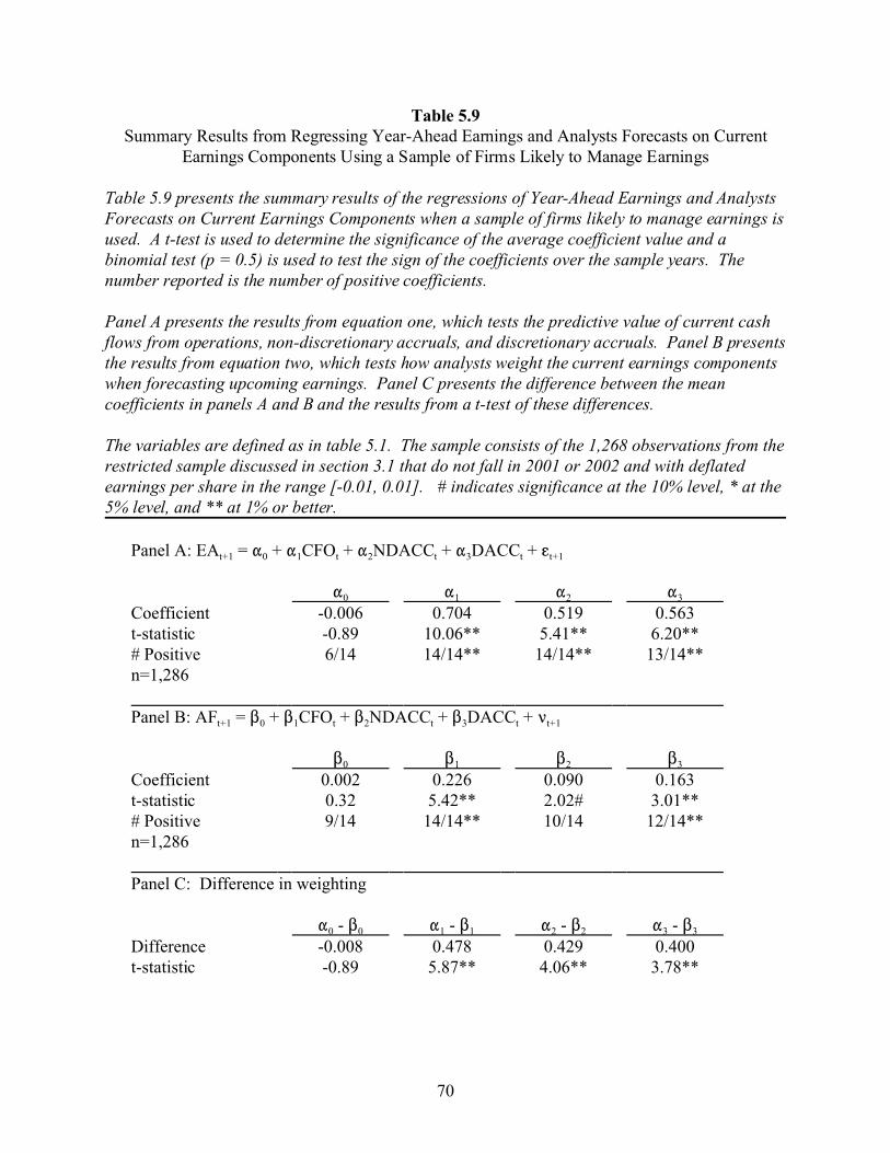
70

Table 5.9Summary Results from Regressing Year-Ahead Earnings and Analysts Forecasts on Current

Earnings Components Using a Sample of Firms Likely to Manage Earnings

Table 5.9 presents the summary results of the regressions of Year-Ahead Earnings and AnalystsForecasts on Current Earnings Components when a sample of firms likely to manage earnings isused. A t-test is used to determine the significance of the average coefficient value and abinomial test (p = 0.5) is used to test the sign of the coefficients over the sample years. Thenumber reported is the number of positive coefficients.

Panel A presents the results from equation one, which tests the predictive value of current cashflows from operations, non-discretionary accruals, and discretionary accruals. Panel B presentsthe results from equation two, which tests how analysts weight the current earnings componentswhen forecasting upcoming earnings. Panel C presents the difference between the meancoefficients in panels A and B and the results from a t-test of these differences.

The variables are defined as in table 5.1. The sample consists of the 1,268 observations from therestricted sample discussed in section 3.1 that do not fall in 2001 or 2002 and with deflatedearnings per share in the range [-0.01, 0.01]. # indicates significance at the 10% level, * at the5% level, and ** at 1% or better.

Panel A: EAt+1 = "0 + "1CFOt + "2NDACCt + "3DACCt + gt+1

"0 "1 "2 "3

Coefficient -0.006 0.704 0.519 0.563t-statistic -0.89 10.06** 5.41** 6.20**# Positive 6/14 14/14** 14/14** 13/14**n=1,286 Panel B: AFt+1 = $0 + $1CFOt + $2NDACCt + $3DACCt + <t+1

$0 $1 $2 $3

Coefficient 0.002 0.226 0.090 0.163t-statistic 0.32 5.42** 2.02# 3.01**# Positive 9/14 14/14** 10/14 12/14**n=1,286 Panel C: Difference in weighting

"0 - $0 "1 - $1 "2 - $2 "3 - $3

Difference -0.008 0.478 0.429 0.400t-statistic -0.89 5.87** 4.06** 3.78**

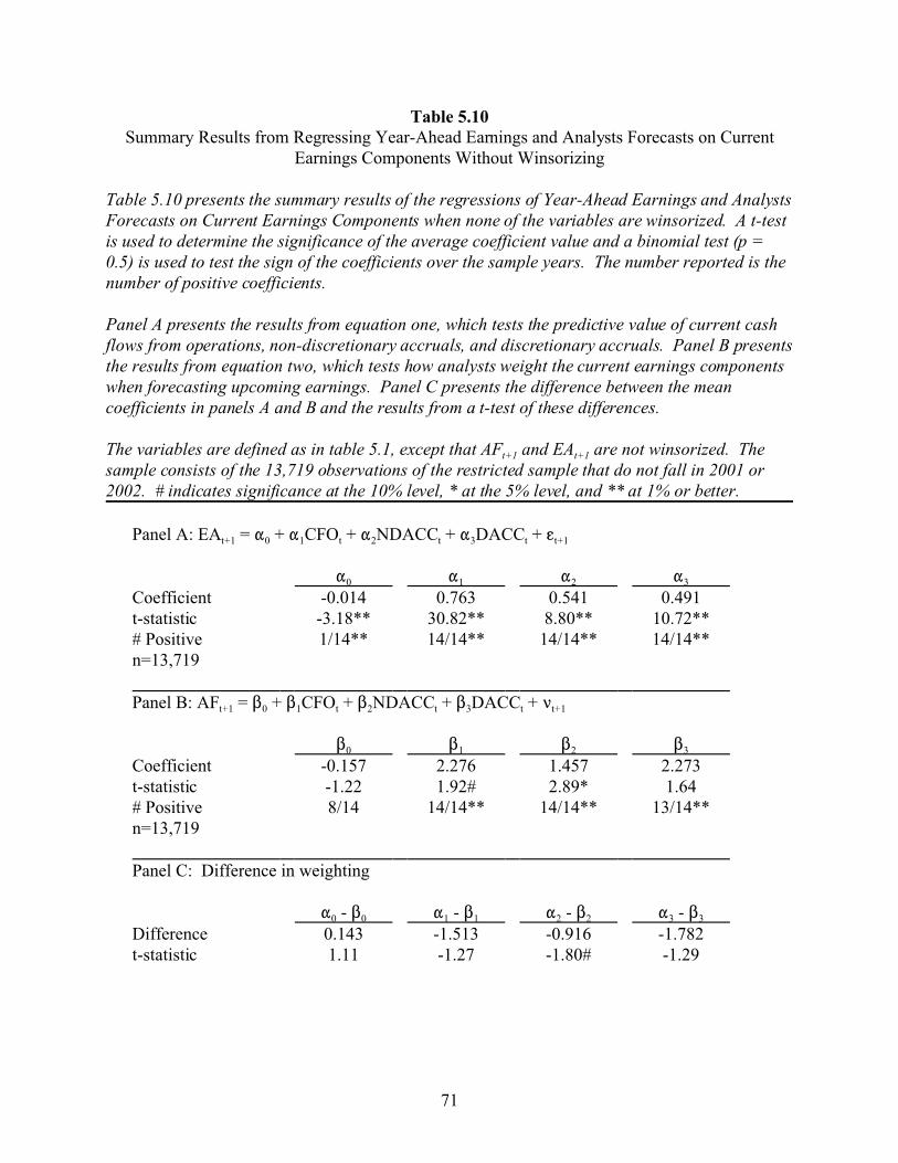
71

Table 5.10Summary Results from Regressing Year-Ahead Earnings and Analysts Forecasts on Current

Earnings Components Without Winsorizing

Table 5.10 presents the summary results of the regressions of Year-Ahead Earnings and AnalystsForecasts on Current Earnings Components when none of the variables are winsorized. A t-testis used to determine the significance of the average coefficient value and a binomial test (p =0.5) is used to test the sign of the coefficients over the sample years. The number reported is thenumber of positive coefficients.

Panel A presents the results from equation one, which tests the predictive value of current cashflows from operations, non-discretionary accruals, and discretionary accruals. Panel B presentsthe results from equation two, which tests how analysts weight the current earnings componentswhen forecasting upcoming earnings. Panel C presents the difference between the meancoefficients in panels A and B and the results from a t-test of these differences.

The variables are defined as in table 5.1, except that AFt+1 and EAt+1 are not winsorized. Thesample consists of the 13,719 observations of the restricted sample that do not fall in 2001 or2002. # indicates significance at the 10% level, * at the 5% level, and ** at 1% or better.

Panel A: EAt+1 = "0 + "1CFOt + "2NDACCt + "3DACCt + gt+1

"0 "1 "2 "3

Coefficient -0.014 0.763 0.541 0.491t-statistic -3.18** 30.82** 8.80** 10.72**# Positive 1/14** 14/14** 14/14** 14/14**n=13,719 Panel B: AFt+1 = $0 + $1CFOt + $2NDACCt + $3DACCt + <t+1

$0 $1 $2 $3

Coefficient -0.157 2.276 1.457 2.273t-statistic -1.22 1.92# 2.89* 1.64# Positive 8/14 14/14** 14/14** 13/14**n=13,719 Panel C: Difference in weighting

"0 - $0 "1 - $1 "2 - $2 "3 - $3

Difference 0.143 -1.513 -0.916 -1.782t-statistic 1.11 -1.27 -1.80# -1.29

72

Table 5.11Summary Results from Regressing Year-Ahead Earnings and Analysts Forecasts on Current

Earnings Components With Double Winsorizing of the AFt+1 Variable

Table 5.11 presents the summary results of the regressions of Year-Ahead Earnings and AnalystsForecasts on Current Earnings Components when analysts forecasts are winsorized twice. A t-test is used to determine the significance of the average coefficient value and a binomial test (p =0.5) is used to test the sign of the coefficients over the sample years. The number reported is thenumber of positive coefficients.

Panel A presents the results from equation one, which tests the predictive value of current cashflows from operations, non-discretionary accruals, and discretionary accruals. Panel B presentsthe results from equation two, which tests how analysts weight the current earnings componentswhen forecasting upcoming earnings. Panel C presents the difference between the meancoefficients in panels A and B and the results from a t-test of these differences.

The variables are defined as in table 5.1, except that AFt+1 was winsorized once when the fullsample was created and again after the product of the mean consensus forecast and the numberof shares used to calculate EPS was calculated. The sample consists of the 13,719 observationsof the restricted sample that do not fall in 2001 or 2002. # indicates significance at the 10%level, * at the 5% level, and ** at 1% or better.

Panel A: EAt+1 = "0 + "1CFOt + "2NDACCt + "3DACCt + gt+1

"0 "1 "2 "3

Coefficient -0.009 0.691 0.490 0.433t-statistic -2.60* 23.29** 8.48** 8.91**# Positive 3/14* 14/14** 14/14** 14/14**n=13,719 Panel B: AFt+1 = $0 + $1CFOt + $2NDACCt + $3DACCt + <t+1

$0 $1 $2 $3

Coefficient 0.001 0.523 0.361 0.307t-statistic 0.20 19.23** 9.78** 9.57**# Positive 8/14 14/14** 14/14** 14/14**n=13,719 Panel C: Difference in weighting

"0 - $0 "1 - $1 "2 - $2 "3 - $3

Difference -0.009 0.168 0.130 0.126t-statistic -2.20* 4.16** 1.89# 2.16**

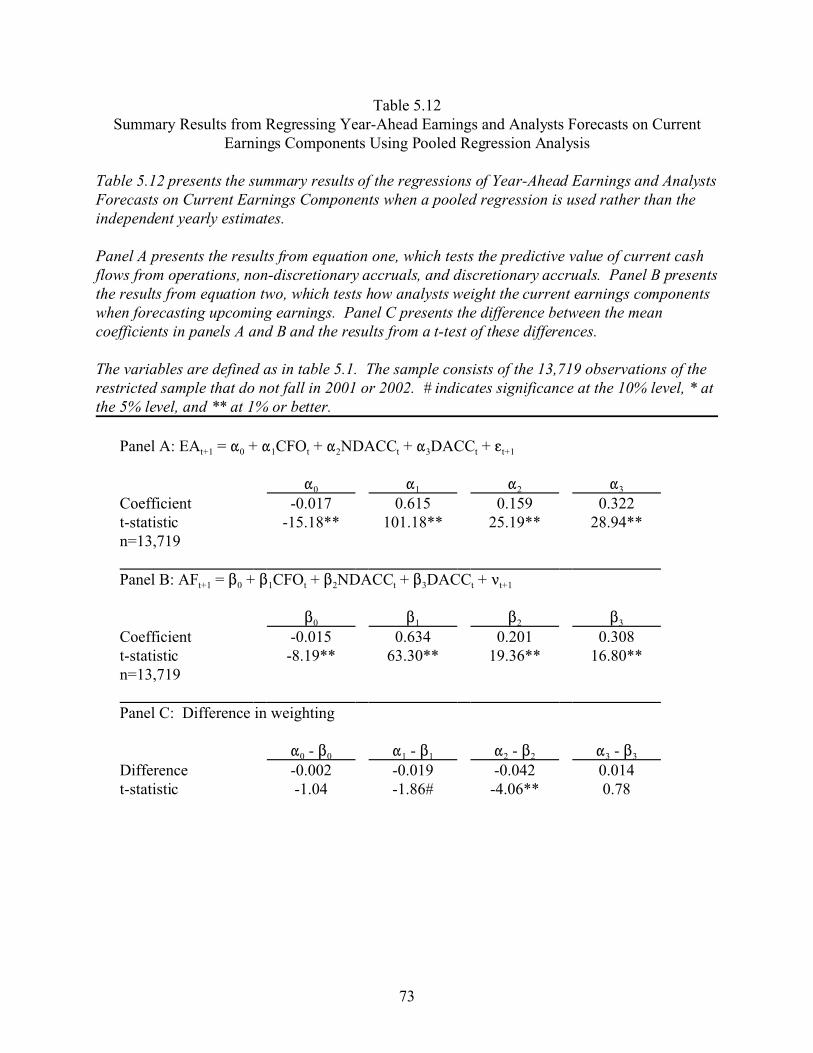
73

Table 5.12Summary Results from Regressing Year-Ahead Earnings and Analysts Forecasts on Current

Earnings Components Using Pooled Regression Analysis

Table 5.12 presents the summary results of the regressions of Year-Ahead Earnings and AnalystsForecasts on Current Earnings Components when a pooled regression is used rather than theindependent yearly estimates.

Panel A presents the results from equation one, which tests the predictive value of current cashflows from operations, non-discretionary accruals, and discretionary accruals. Panel B presentsthe results from equation two, which tests how analysts weight the current earnings componentswhen forecasting upcoming earnings. Panel C presents the difference between the meancoefficients in panels A and B and the results from a t-test of these differences.

The variables are defined as in table 5.1. The sample consists of the 13,719 observations of therestricted sample that do not fall in 2001 or 2002. # indicates significance at the 10% level, * atthe 5% level, and ** at 1% or better.

Panel A: EAt+1 = "0 + "1CFOt + "2NDACCt + "3DACCt + gt+1

"0 "1 "2 "3

Coefficient -0.017 0.615 0.159 0.322t-statistic -15.18** 101.18** 25.19** 28.94**n=13,719 Panel B: AFt+1 = $0 + $1CFOt + $2NDACCt + $3DACCt + <t+1

$0 $1 $2 $3

Coefficient -0.015 0.634 0.201 0.308t-statistic -8.19** 63.30** 19.36** 16.80**n=13,719 Panel C: Difference in weighting

"0 - $0 "1 - $1 "2 - $2 "3 - $3

Difference -0.002 -0.019 -0.042 0.014t-statistic -1.04 -1.86# -4.06** 0.78

74

CHAPTER 6

THE ASSOCIATIONS BETWEEN ANALYST FORECASTS AND REPORTED AND

RESTATED EARNINGS

6.1 The Model

The analysis in chapter five suggests that analysts do not remove the effects of earnings

management from their forecasts. However, an alternative explanation for these results is

analysts’ inability to appropriately weight components of earnings. Prior evidence (Abarbanell

1991, Bradshaw, Richardson and Sloan 2001, Plumlee 2003, Ramnath 2002, Shane and Brous

2001, and Weber 2005) suggests that analysts can have difficulty interpreting individual pieces of

information. On the other hand, analysts’ overall forecasts tend be relatively accurate and

improve over the course of the year (Barron, Byard and Kim 2002, Brown 1997, Brown and Han

1992, Crichfield, Dyckman and Lakonishok 1978, and Hope 2003). This implies that the

association between analysts’ forecasts and total earnings (rather than components of earnings)

should be considered. Ideally, the associations between the forecast and earnings with and

without earnings management would be computed and then compared. This chapter proposes

and tests the following model for this purpose:

Analyst Forcastst = 80 + 81Managed Earningst + *t (4)

Analyst Forcastst = N0 + N1Unmanaged Earningst + Jt (5)

where Analyst Forcastst is the mean consensus analyst forecast of earnings per share at time t

times the number of shares used to calculate EPS (Compustat data item 54), Managed Earningst

is reported earnings before extra items at time t (Compustat data item123), and Unmanaged

75

Earningst is restated earnings before extra items (Compustat data item 118). All three variables

are deflated by lagged assets. In order to determine whether managed or unmanaged earnings is

more highly associated with analysts forecasts I use a Vuong test, which is described by Dechow

(1994). The Vuong (1989) test uses a z-statistic to assess which equation (four or five) has the

lower sum of squared residuals. The earnings definition in the equation with the lower sum of

squared errors is more highly associated with analyst forecasts.

The analysis is based on three assumptions. First, I assume that analysts convey their

understanding of earnings management in their analyst forecast, rather than in other disclosures.

This assumption is consistent with Schipper (1991). Second, I assume that analysts do not issue

separate forecasts of pre-managed earnings. This is consistent with Abarbanell and Lehavy

(2003), Burgstahler and Eames (2003), and Liu (2005). Third, and most importantly, I assume

that restated earnings has been purged of earnings management. This is consistent with

Erickson, Hanlon and Maydew (2004), Jones, Krishnan and Melendez (2006), and Palmrose,

Richardson and Scholz (2004).

6.2 Predictions

I assume that reported earnings include earnings management and restated earnings do

not. This implies that if analysts include earnings management in their forecasts, then analysts’

forecasts will be more highly associated with reported earnings than they are with restated

earnings. This is hypothesis four:

H4: If analysts include the effects of earnings management in their forecast, then theassociation between analyst forecasts and reported earnings will exceed theassociation between analyst forecasts and restated earnings.

76

The converse will also be true. If analysts exclude earnings management from their

forecasts, then analysts’ forecasts will be more highly associated with restated earnings than they

are with reported earnings. This is hypothesis five:

H5: If analysts remove the effects of earnings management from their forecast, thenthe association between analyst forecasts and restated earnings will exceed theassociation between analyst forecasts and reported earnings.

6.3 Sample Selection and Summary Statistics

To test hypotheses four and five, I start with the full sample described in chapter three

and detailed in table 3.1. I retain only the observations with data available from Compustat on

restated earnings and lagged assets. After truncating the sample at the 1st and 99th percentile of

reported earnings, restated earnings, and mean consensus analyst forecasts, 15,158 observations

remain. I refer to this set of observations as the ‘restatement sample.’

Compustat gives four reasons for restated earnings: discontinued operations, mergers and

acquisitions, earnings management, and errors in managers’ original estimates. Since I use

income before extra items, restatements due to discontinued operations will not enter my sample.

However, the sample could include restatements due to mergers and acquisitions or legitimate

errors in estimates. I partially address this issue by removing firms that report merger or

acquisition activity for the year. This leaves restatements due to errors in estimates in the

sample. Unfortunately, Compustat does not differentiate between errors in estimates and

earnings management. This restriction reduces the sample to 8,139 firm-years. I refer to this set

of observations as the ‘restricted restatement sample.’ Table 6.1 contains a summary of the

sample selection procedure.

77

Table 6.2 presents summary statistics for the restatement and restricted restatement

samples. The variables are defined as follows: total assets is Compustat data item 6; the number

of analysts is the number that participated in creating each consensus forecast, as reported by

IBES; analyst forecast is the mean consensus forecast reported by IBES multiplied by the number

of shares used to calculate EPS (Compustat data item 54); reported earnings is income before

extra items (Compustat data item 123); and restated earnings is income before extra items

(restated) (Compustat data item 118). Analyst forecast, reported earnings, and restated earnings

are deflated by lagged total assets.

The firms in the restricted restatement sample are smaller than those in the restatement

sample ($4,001.7 million versus $6,608.7 million, p < 0.001). This is not surprising, because

smaller firms are more likely to have financial difficulties leading them to manage earnings while

larger firms are more likely to be involved in mergers and acquisitions. Also consistent with

their smaller size, the firms in the restricted restatement sample are followed by fewer analysts on

average (6.4) than firms in the restatement sample (7.5) (p < 0.001).

6.4 Results

Before proceeding to the estimation of equations four and five, I compute simple

correlations between the analyst forecasts and reported and restated earnings. The correlations

are presented in table 6.3. Panel A reports results for the restatement sample. The correlation

between reported earnings and analysts’ forecasts is 0.837, and the correlation between restated

earnings and analysts’ forecasts is 0.832. Panel B presents similar results for the restricted

restatement sample (0.873 and 0.867 for reported and restated earnings, respectively). The

correlation between analyst forecasts and reported earnings is higher than the correlation between

78

analyst forecasts and restated earnings for both samples (p = 0.0755 for the restatement sample

and p = 0.016 for the restricted restatement sample, one-tailed test). This is consistent with the

prediction of hypothesis four that analysts include earnings management in their forecasts.

Table 6.4 presents the results of estimating equations four and five. Panels A and B report

coefficients, adjusted R2 values, and observations for equations four and five, respectively. In

both the restatement sample (column one) and the restricted restatement sample (column two),

the adjusted R2 values are higher for reported earnings than restated earnings. In addition, the

coefficient on reported earnings (panel A) is closer to one than the coefficient on restated

earnings (panel B) for both samples.

Panel C reports the results of the Vuong test, which is used to assess the statistical

significance of the differences in both adjusted R2 and coefficient values. If analysts include

earnings management in their forecasts, then their forecasts should be more highly associated

with reported than restated earnings (consistent with hypothesis four) and the z-statistic from the

Vuong test will be negative. If, on the other hand, analysts remove earnings management from

their forecasts, their forecasts should be more highly associated with restated than reported

earnings and the z-statistic from the Vuong test will be positive. This would support hypothesis

five. Consistent with hypothesis four, the z-statistic is -2.48 for the restatement sample and -2.51

for the restricted restatement sample. These significantly negative results suggest that analysts

forecasts are more highly associated with reported earnings than they are with restated earnings,

indicating that analysts include the effects of earnings management in their forecasts. Thus,

hypothesis five is rejected in favor of hypothesis four.

79

6.5 Sensitivity Tests

6.5.1 Alternative samples

In order to ensure that these results are not dependent on the sample of mean consensus

forecasts, I repeat the Vuong test using three of the alternative samples discussed in section 5.7.

First, I use a sample of median consensus forecasts; second, a sample of last available forecasts;

and third, a sample of individual forecasts from the IBES detail sample. I do not use a sample of

quarterly observations because Compustat does not provide quarterly restatement data. For each

sample, I begin with a set of annual earnings forecasts for all December year-end, U.S. firms

during the period 1988-2004. I then remove those observations made more than 30 days prior to

the fiscal year end and those without the needed restatement and lagged asset data. Finally, I

truncate the analyst forecasts and reported and restated earnings distributions at the 1st and 99th

percentiles. The results are presented in table 6.5 for the median sample, table 6.6 for the last

available forecast sample, and table 6.7 for the detail file sample. Except for the insignificant z-

statistic for the restatement sample using the last available forecast (table 6.6, column one), the

results are consistent with those presented in table 6.4.

6.5.2 Removing observations from 2001 and 2002

Although the restatement and restricted restatement samples used in this chapter are

different from the restricted sample used in chapter five, I replicate the analysis after removing

the observations from 2002 and 2003 to ensure that the anomalies found in tables 5.2 and 5.3 do

not affect the results of the current tests. This restriction reduces the restatement and restricted

restatement samples to 10,260 and 5,605 observations, respectively. The results, presented in

table 6.8, are consistent with those presented in table 6.4. Since the anomalies in the 2001 and

80

2002 data involve year-ahead earnings as well as the current earnings components, I also

replicated the tests after removing the observations from 2002 and 2003. The results

(untabulated) are also consistent with those in table 6.4.

6.6 Conclusions

This chapter examines the association between analyst forecasts and reported and restated

earnings. The evidence suggests that analyst forecasts are more highly associated with reported

earnings than they are with restated earnings. I interpret this as meaning that analysts include,

rather than remove, the effects of earnings management in their forecasts. This is consistent with

the results presented in chapter five and the findings of Burgstahler and Eames (2003).

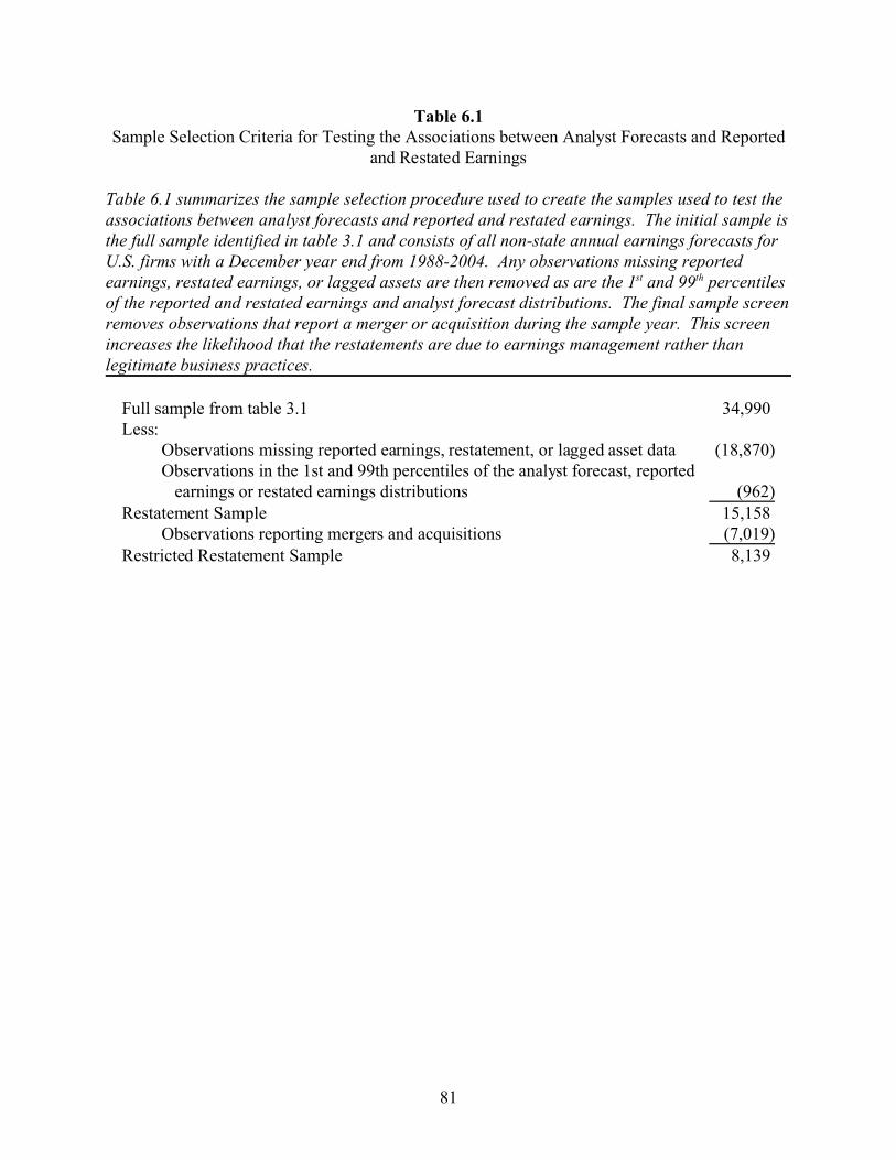
81

Table 6.1Sample Selection Criteria for Testing the Associations between Analyst Forecasts and Reported

and Restated Earnings

Table 6.1 summarizes the sample selection procedure used to create the samples used to test theassociations between analyst forecasts and reported and restated earnings. The initial sample isthe full sample identified in table 3.1 and consists of all non-stale annual earnings forecasts forU.S. firms with a December year end from 1988-2004. Any observations missing reportedearnings, restated earnings, or lagged assets are then removed as are the 1st and 99th percentilesof the reported and restated earnings and analyst forecast distributions. The final sample screenremoves observations that report a merger or acquisition during the sample year. This screenincreases the likelihood that the restatements are due to earnings management rather thanlegitimate business practices.

Full sample from table 3.1 34,990 Less:

Observations missing reported earnings, restatement, or lagged asset data (18,870)Observations in the 1st and 99th percentiles of the analyst forecast, reported

earnings or restated earnings distributions (962)Restatement Sample 15,158

Observations reporting mergers and acquisitions (7,019)Restricted Restatement Sample 8,139

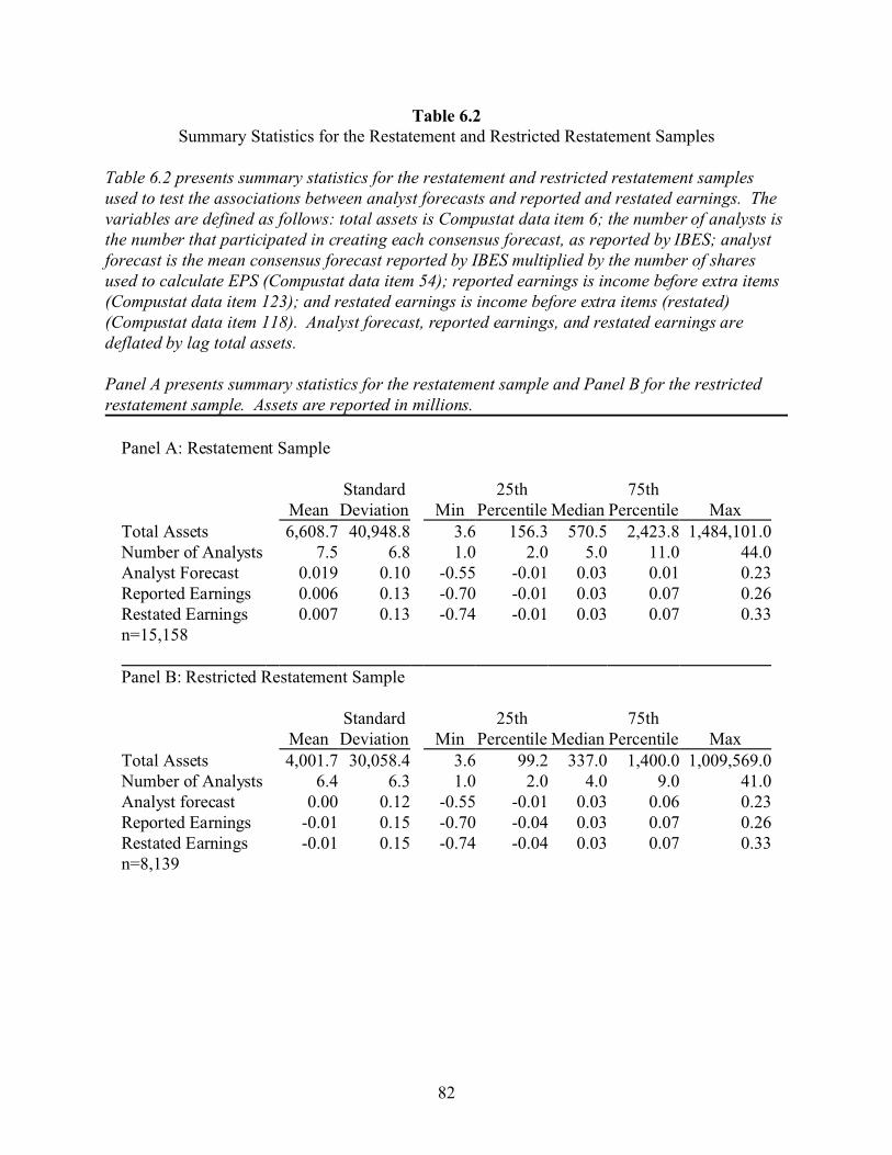
82

Table 6.2Summary Statistics for the Restatement and Restricted Restatement Samples

Table 6.2 presents summary statistics for the restatement and restricted restatement samplesused to test the associations between analyst forecasts and reported and restated earnings. Thevariables are defined as follows: total assets is Compustat data item 6; the number of analysts isthe number that participated in creating each consensus forecast, as reported by IBES; analystforecast is the mean consensus forecast reported by IBES multiplied by the number of sharesused to calculate EPS (Compustat data item 54); reported earnings is income before extra items(Compustat data item 123); and restated earnings is income before extra items (restated)(Compustat data item 118). Analyst forecast, reported earnings, and restated earnings aredeflated by lag total assets.

Panel A presents summary statistics for the restatement sample and Panel B for the restrictedrestatement sample. Assets are reported in millions.

Panel A: Restatement Sample

Standard 25th 75thMean Deviation Min Percentile Median Percentile Max

Total Assets 6,608.7 40,948.8 3.6 156.3 570.5 2,423.8 1,484,101.0Number of Analysts 7.5 6.8 1.0 2.0 5.0 11.0 44.0Analyst Forecast 0.019 0.10 -0.55 -0.01 0.03 0.01 0.23Reported Earnings 0.006 0.13 -0.70 -0.01 0.03 0.07 0.26Restated Earnings 0.007 0.13 -0.74 -0.01 0.03 0.07 0.33n=15,158 Panel B: Restricted Restatement Sample

Standard 25th 75thMean Deviation Min Percentile Median Percentile Max

Total Assets 4,001.7 30,058.4 3.6 99.2 337.0 1,400.0 1,009,569.0Number of Analysts 6.4 6.3 1.0 2.0 4.0 9.0 41.0Analyst forecast 0.00 0.12 -0.55 -0.01 0.03 0.06 0.23Reported Earnings -0.01 0.15 -0.70 -0.04 0.03 0.07 0.26Restated Earnings -0.01 0.15 -0.74 -0.04 0.03 0.07 0.33n=8,139

83

Table 6.3Correlations between Analyst Forecasts and Reported and Restated Earnings

Table 6.3 presents the correlations between analyst forecasts and reported and restated earningsfor the restatement and restricted restatement samples used to test the associations betweenanalyst forecasts and reported and restated earnings. The variables are defined as follows:analyst forecast is the mean consensus forecast reported by IBES multiplied by the number ofshares used to calculate EPS (Compustat data item 54); reported earnings is income before extraitems (Compustat data item 123); and restated earnings is income before extra items (restated)(Compustat data item 118). All three variables are deflated by lagged total assets.

Panel A presents correlations for the restatement sample and Panel B for the restrictedrestatement sample.

Panel A: Restatement Sample

AnalystForecasts

Reported EA 0.837(Probability) (<0.0001)

Restated EA 0.832(Probability) (<0.0001)

n=15,158 Panel B: Restricted Restatement Sample

AnalystForecasts

Reported EA 0.873(Probability) (<0.0001)

Restated EA 0.867(Probability) (<0.0001)

n=8,139

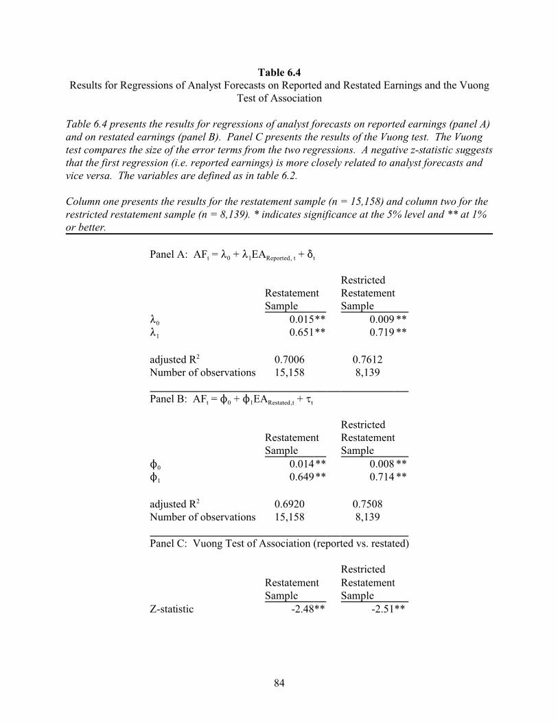
84

Table 6.4Results for Regressions of Analyst Forecasts on Reported and Restated Earnings and the Vuong

Test of Association

Table 6.4 presents the results for regressions of analyst forecasts on reported earnings (panel A)and on restated earnings (panel B). Panel C presents the results of the Vuong test. The Vuongtest compares the size of the error terms from the two regressions. A negative z-statistic suggeststhat the first regression (i.e. reported earnings) is more closely related to analyst forecasts andvice versa. The variables are defined as in table 6.2.

Column one presents the results for the restatement sample (n = 15,158) and column two for therestricted restatement sample (n = 8,139). * indicates significance at the 5% level and ** at 1%or better.

Panel A: AFt = 80 + 81EAReported, t + *t

RestrictedRestatementSample

RestatementSample

80 0.015** 0.009 **81 0.651** 0.719 **

adjusted R2 0.7006 0.7612Number of observations 15,158 8,139 Panel B: AFt = N0 + N1EARestated,t + Jt

RestrictedRestatementSample

RestatementSample

N0 0.014** 0.008 **N1 0.649** 0.714 **

adjusted R2 0.6920 0.7508Number of observations 15,158 8,139 Panel C: Vuong Test of Association (reported vs. restated)

RestrictedRestatementSample

RestatementSample

Z-statistic -2.48** -2.51**

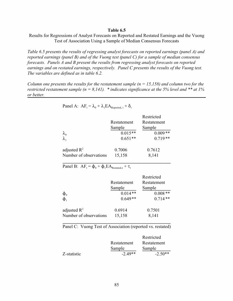
85

Table 6.5Results for Regressions of Analyst Forecasts on Reported and Restated Earnings and the Vuong

Test of Association Using a Sample of Median Consensus Forecasts

Table 6.5 presents the results of regressing analyst forecasts on reported earnings (panel A) andreported earnings (panel B) and of the Vuong test (panel C) for a sample of median consensusforecasts. Panels A and B present the results from regressing analyst forecasts on reportedearnings and on restated earnings, respectively. Panel C presents the results of the Vuong test. The variables are defined as in table 6.2.

Column one presents the results for the restatement sample (n = 15,158) and column two for therestricted restatement sample (n = 8,141). * indicates significance at the 5% level and ** at 1%or better.

Panel A: AFt = 80 + 81EAReported, t + *t

RestrictedRestatementSample

RestatementSample

80 0.015** 0.009 **81 0.651** 0.719 **

adjusted R2 0.7006 0.7612Number of observations 15,158 8,141 Panel B: AFt = N0 + N1EARestated,t + Jt

RestrictedRestatementSample

RestatementSample

N0 0.014** 0.008 **N1 0.649** 0.714 **

adjusted R2 0.6914 0.7501Number of observations 15,158 8,141 Panel C: Vuong Test of Association (reported vs. restated)

RestrictedRestatementSample

RestatementSample

Z-statistic -2.49** -2.50**

86

Table 6.6Results for Regressions of Analyst Forecasts on Reported and Restated Earnings and the Vuong

Test of Association Using a Sample of Last Available Analyst Forecasts

Table 6.6 presents the results of regressing analyst forecasts on reported earnings (panel A) andreported earnings (panel B) and of the Vuong test (panel C) for a sample of last availableanalyst forecasts. Panels A and B present the results from regressing analyst forecasts onreported earnings and on restated earnings, respectively. Panel C presents the results of theVuong test. The variables are defined as in table 6.2.

Column one presents the results for the restatement sample (n = 8,909) and column two for therestricted restatement sample (n = 4,497). * indicates significance at the 5% level and ** at 1%or better.

Panel A: AFt = 80 + 81EAReported, t + *t

RestrictedRestatementSample

RestatementSample

80 0.016** 0.009 **81 0.621** 0.703 **

adjusted R2 0.6834 0.7664Number of observations 8,909 4,497 Panel B: AFt = N0 + N1EARestated,t + Jt

RestrictedRestatementSample

RestatementSample

N0 0.016** 0.009 **N1 0.616** 0.691 **

adjusted R2 0.6709 0.746Number of observations 8,909 4,497 Panel C: Vuong Test of Association (reported vs. restated)

RestrictedRestatementSample

RestatementSample

Z-statistic -1.80** -2.08**

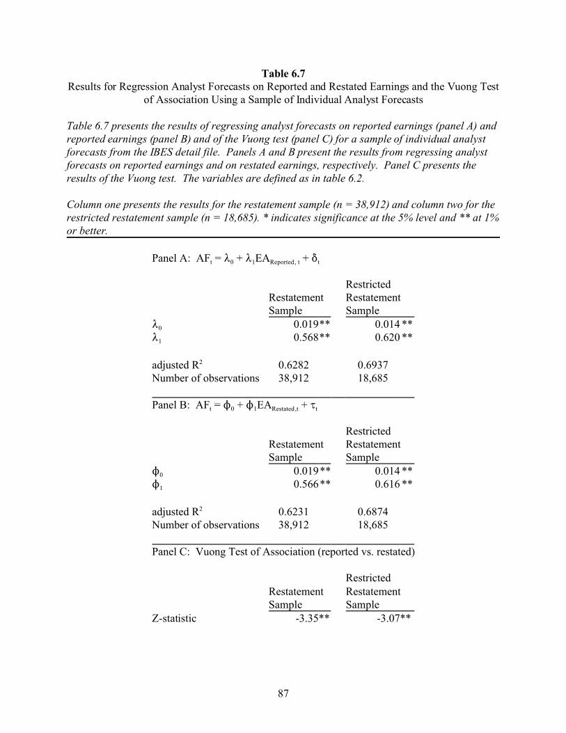
87

Table 6.7Results for Regression Analyst Forecasts on Reported and Restated Earnings and the Vuong Test

of Association Using a Sample of Individual Analyst Forecasts

Table 6.7 presents the results of regressing analyst forecasts on reported earnings (panel A) andreported earnings (panel B) and of the Vuong test (panel C) for a sample of individual analystforecasts from the IBES detail file. Panels A and B present the results from regressing analystforecasts on reported earnings and on restated earnings, respectively. Panel C presents theresults of the Vuong test. The variables are defined as in table 6.2.

Column one presents the results for the restatement sample (n = 38,912) and column two for therestricted restatement sample (n = 18,685). * indicates significance at the 5% level and ** at 1%or better.

Panel A: AFt = 80 + 81EAReported, t + *t

RestrictedRestatementSample

RestatementSample

80 0.019** 0.014 **81 0.568** 0.620 **

adjusted R2 0.6282 0.6937Number of observations 38,912 18,685 Panel B: AFt = N0 + N1EARestated,t + Jt

RestrictedRestatementSample

RestatementSample

N0 0.019** 0.014 **N1 0.566** 0.616 **

adjusted R2 0.6231 0.6874Number of observations 38,912 18,685 Panel C: Vuong Test of Association (reported vs. restated)

RestrictedRestatementSample

RestatementSample

Z-statistic -3.35** -3.07**

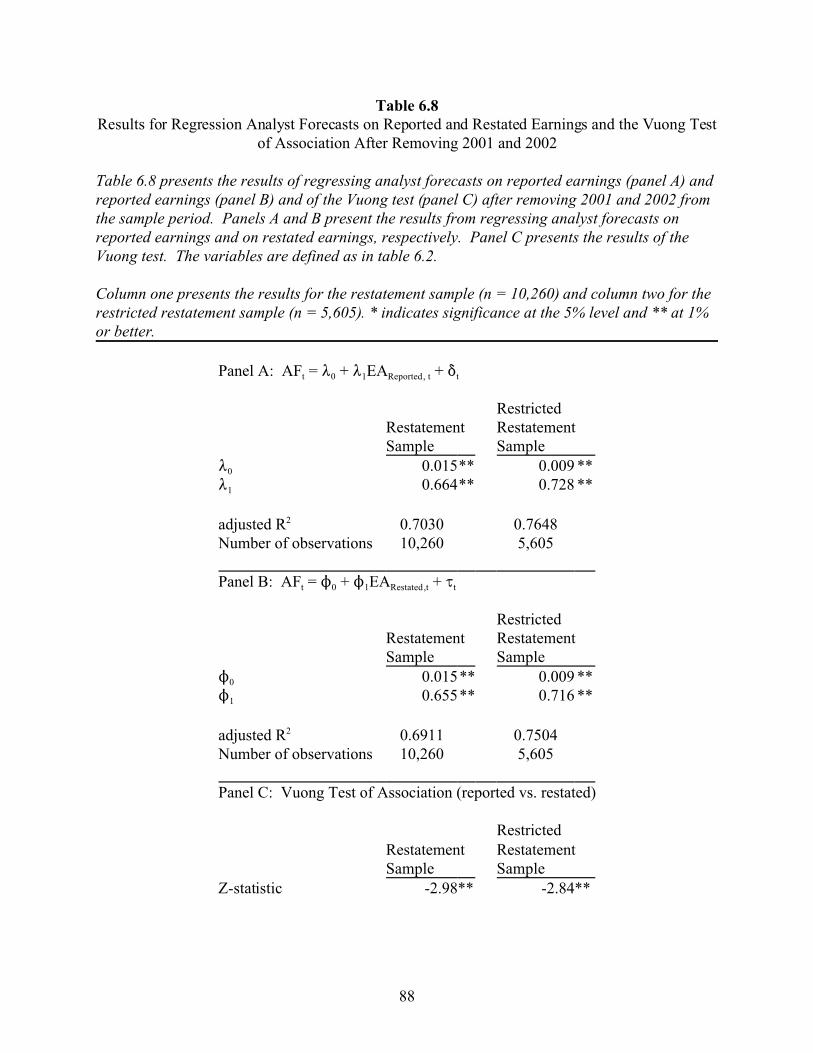
88

Table 6.8Results for Regression Analyst Forecasts on Reported and Restated Earnings and the Vuong Test

of Association After Removing 2001 and 2002

Table 6.8 presents the results of regressing analyst forecasts on reported earnings (panel A) andreported earnings (panel B) and of the Vuong test (panel C) after removing 2001 and 2002 fromthe sample period. Panels A and B present the results from regressing analyst forecasts onreported earnings and on restated earnings, respectively. Panel C presents the results of theVuong test. The variables are defined as in table 6.2.

Column one presents the results for the restatement sample (n = 10,260) and column two for therestricted restatement sample (n = 5,605). * indicates significance at the 5% level and ** at 1%or better.

Panel A: AFt = 80 + 81EAReported, t + *t

RestrictedRestatementSample

RestatementSample

80 0.015** 0.009 **81 0.664** 0.728 **

adjusted R2 0.7030 0.7648Number of observations 10,260 5,605 Panel B: AFt = N0 + N1EARestated,t + Jt

RestrictedRestatementSample

RestatementSample

N0 0.015** 0.009 **N1 0.655** 0.716 **

adjusted R2 0.6911 0.7504Number of observations 10,260 5,605 Panel C: Vuong Test of Association (reported vs. restated)

RestrictedRestatementSample

RestatementSample

Z-statistic -2.98** -2.84**

89

CHAPTER 7

TESTS OF THE LAST MINUTE EARNINGS MANAGEMENT HYPOTHESIS

7.1 Last Minute Manipulations

The results in chapters five and six suggest that analysts include earnings management in

their forecasts. However, they do not explain why Abarbanell and Lehavy (2003) find

asymmetries in the forecast error distribution consistent with analysts removing the effects of

earnings management. One explanation for Abarbanell and Lehavy’s results is that analysts are

consistently mistaken in anticipating earnings management for a significant number of firms.

This explanation is not compelling for two reasons. First, although anticipating earnings

management is undoubtedly difficult (Fischer and Verrecchia 2000), there is evidence that

analysts are capable of doing so (Burgstahler and Eames 2003, Liu 2005). Second, an

explanation based on analyst error is inconsistent with the pattern of the asymmetries. If analysts

make mistakes in predicting earnings management, then their mistakes should be random. In

terms of the forecast error distribution, this means a roughly equal number of observations both

above and below zero, and roughly symmetric tails. However, this is not the pattern observed in

figure 3.2.

Brown (1998) provides an alternative explanation for the existence of the asymmetries

documented by Abarbanell and Lehavy (2003). He observes that managers provide information

throughout the fiscal period that analysts use to make and revise their earnings forecasts. At the

end of the period, however, the situation is reversed. Analysts make their final forecasts of

earnings before managers issue their final earnings announcement. In the period between the

90

final analyst forecasts and the earnings announcement, managers can make ‘last minute’

manipulations so that reported earnings meet-or-beat market expectations. The sequence of

events is presented in figure 7.1. Even if analysts try to include earnings management in their

forecasts, last minute manipulations could lead to asymmetries such as those described by

Abarbanell and Lehavy (2003). Last minute manipulation to meet expectations has been

documented in a tax setting by Dhaliwal, Gleason and Mills (2003).

7.2 Proxy for Earnings Prior to Last Minute Manipulations

To test the last minute manipulation explanation, I examine whether the level of earnings

management increases when analysts raise investor expectations. I use a sample of management

forecasts of earnings to proxy for the level of earnings prior to last minute manipulations. I

assume that management forecasts of earnings include both pre-managed earnings and the

earnings manipulations managers plan to make before the release of the analyst forecast. This

assumption is consistent with prior research. For example, Kasznik (1999) finds that firms

include earnings management to reach their management forecast. Ke, Huddart and Petroni

(2003) show that managers know what their important accounting disclosures, such as earnings

announcements, will be in advance of the actual disclosure.

7.3 Sample Selection and Summary Statistics

I construct a sample of point and range management forecasts of annual earnings from

First Call from 1985 to 2004. If the forecast is a range, I record the upper bound of the range in

order to increase the probability that the management forecast contains both pre-managed

earnings and planned earnings management. I restrict the sample to management forecasts made

91

within 20 days of the end of the period to increase the probability that the forecast contains pre-

managed earnings and planned earnings management, but not last minute manipulations. Finally,

I require each observation to have an analyst forecast issued after the management forecast, a

reported earnings number available from the IBES consensus database, and a beginning of the

period stock price available from CRSP. I winsorize the management and analyst forecasts at the

1st and 99th percentiles to control for outliers. These sample screens result in 312 management

forecasts. The sample selection procedure is summarized in table 7.1.

Table 7.2, panel A, presents summary statistics for the management forecast sample.

Overall, the sample consists of relatively large firms (mean total assets of $13,654 million) that

are followed, on average, by five analysts. On average, analyst forecasts are significantly higher

than management forecasts (p < 0.001). This suggests that analysts are more likely to remove

transitory bad news from their earnings forecasts (Barth et al. 2001) than managers (Pownall and

Waymire 1989, Skinner 1994).

7.4 Developing the Model

To test for the existence of last minute manipulations, I first split the sample according to

whether or not analysts raise market expectations. I assume that analysts raise expectations when

the analyst forecast is higher than the management forecast. Conversely, when the analyst

forecast is lower than the management forecast, I assume analysts have lowered expectations.

When analysts raise market expectations, managers have incentives to use last minute

manipulations to increase reported earnings beyond the initially planned level indicated by the

management forecast. This leads to hypothesis six.

H6: When the analyst forecast exceeds the management forecast, reported earningswill also exceed the management forecast.

92

On the other hand, if analysts lower market expectations, then managers will not have incentives

to raise reported earnings. Instead, they will either ‘take a bath’ to improve their ability to

manage earnings in the future (Barton and Simko 2002, DeFond and Park 1997) or will exactly

meet their management forecast to improve their credibility (Skinner 1994, Tucker 2004). This

leads to hypothesis seven.

H7: When the analyst forecast falls below the management forecast, reported earningswill not exceed the management forecast.

7.5 Results

Table 7.3 presents the results of a two by two chi-squared test of hypotheses six and

seven. The rows partition the sample according to managers’ incentives to engage in last minute

earnings management. The first row contains observations where there is no incentive to

increase earnings, because the analyst forecast does not exceed the management forecast. For

these observations, managers are predicted to either meet their management forecast or ‘take a

bath.’ The second row contains observations where there is an incentive to increase earnings,

because the analyst forecast is above the management forecast. For these observations, managers

are predicted to report earnings that are higher than the management forecast. The columns

partition the sample according to the effect of the last minute manipulations. The first column

contains observations where earnings equal or fall below their management forecast. The second

column contains observations where earnings exceed the management forecast. Hypothesis six

predicts that when the analyst forecast exceeds the management forecast, managers will perform

last minute manipulations to increase reported earnings above the planned earnings level prior to

last minute manipulations. As a result, reported earnings will exceed the management forecast.

Hypothesis seven predicts that when the management forecast exceeds the analyst forecast,

93

managers will either perform no last minute earnings management or will use last minute

manipulations to lower reported earnings below the initially planned level. In this case, reported

earnings will equal or miss the management forecast.

For a sample of 312, the expected number of observations in each cell is 78. As predicted

by hypothesis six, almost half of the observations (147) increased their reported earnings after

receiving an analyst forecast that exceeded their management forecast. In addition, a higher than

expected number of firms (93) missed or met their management forecast when the analyst

forecast was below the management forecast, consistent with hypothesis seven. The chi-squared

statistic of 97.83 is significant at the 0.0001 level.

One impediment to this analysis is the possibility that managers issue their forecasts

below their expectations in order to beat them (Gigler and Hemmer 2001 and Matsumoto 2002).

In this case, management forecasts understate managers' expected earnings prior to last minute

manipulations. While the use of the upper bound of the range forecast should provide some

control for this possibility, I also replicate my tests after increasing each management forecast by

$0.01. The use of $0.01 is based on the finding of Kasznik (1999) that firms that beat their

management forecast do so by an average of $0.01. The results, presented in Panel B of table

7.3, are virtually identical to those in Panel A. I also performed the analysis after adding $0.02

and $0.05 to the management forecast. The results (untabulated) are also quite similar to those

presented in table 7.3.

94

7.6 Sensitivity Analysis

7.6.1 Alternative Sample

Soffer, Thiagarajan and Walther (2000) and Tan, Libby and Hunton (2002) argue that if

managers use their forecasts to manage expectations, they are most likely to do so with forecasts

issued immediately prior to the fiscal year end. This is a concern because my sample consists of

management forecasts made in the last 20 days of the fiscal period. To address this issue, I

construct an alternative sample of management forecasts issued after the end of the fiscal period.

I assume that these forecasts are pre-announcements of earnings rather than attempts to

manipulate expectations, since prior research finds that forecasts issued after the close of the

fiscal period consist of primarily good news (Baginski, Hassell and Waymire 1994), while

expectations management normally consists of reporting bad news (Soffer, et al. 2000). The

resulting sample consists of 597 pre-announcements.

The results presented in panel A of table 7.4, based on reported pre-announcements, are

qualitatively identical to those in panel A of table 7.3, and support both hypothesis six and

hypothesis seven. However, panel B of table 7.4 shows that the results for the pre-announcement

sample are sensitive to increasing the management forecast by $0.01. After this adjustment,

hypothesis seven is still supported, but hypothesis six is not. The implication is that last minute

manipulations that increase earnings are less common following management forecasts that occur

after the close of the fiscal year. This might be due to increased auditor scrutiny of earnings

manipulations when earnings have been pre-announced.

95

7.6.2 The management forecast value of range forecasts

One possible explanation for the high number of observations that missed or met their

management forecast when the analyst forecast was below the management forecast is the use of

the upper bound of range forecasts as the management forecast value. While the use of the upper

bound increases the likelihood that the management forecast contains both pre-managed earnings

and planned earnings management, it could distort incentives to engage in last minute

manipulations, since market expectations prior to the analyst forecast are likely to lie within the

range of the management forecast rather than at the upper bound. For example, for a firm that

issues a range forecast of $1.50 to $2.00, an analyst forecast of $1.95 will raise market

expectations if the market is focused on the midpoint ($1.75) or the lower bound ($1.50) instead

of the upper bound ($2.00). However, the current classification method would place the

observations in the low earnings management incentives category. This misclassification could

bias the results in favor of hypothesis seven. In order to control for this possibility, I replicate

my tests after removing the range forecasts from the sample. I also replicate the tests leaving the

range forecasts in the sample, but using, alternatively, the lower bound and the midpoint as the

point estimate for analysis.

Table 7.5 presents the results of the chi-squared tests after removing the range forecasts.

The resulting sample consists of 86 point forecasts. The expected number of observations in

each cell is 21.5. Panel A of table 7.5 reports that more than half of the observations (44)

increase their reported earnings after receiving an analyst forecast that exceeds their management

forecast, consistent with hypothesis six. In addition, a higher than expected number of

observations (26) met or missed their management forecast when the analyst forecast did not

96

exceed their management forecast, consistent with hypothesis seven. The results after adding

$0.01 to the management forecast, shown in panel B, are qualitatively similar.

Tables 7.6 and 7.7 present the results after defining the management forecast value of the

range forecasts as the lower bound and the midpoint of the range, respectively. The expected

number of observations in each cell is 78. Overall, the results are consistent with those in table

7.3. The only exception is that panel A of tables 7.6 shows no evidence that a higher than

expected number of firms missed or met their forecasts when the analyst forecast was below the

management forecast, contrary to hypothesis seven.

7.6.3 Removing observations from 2001 and 2002

Although the management forecast sample used in the current analysis is different from

the analyst forecast sample used in chapter five, I replicate the chi-squared tests after removing

the observations from 2001 and 2002 to ensure that the anomalies documented in tables 5.2 and

5.3 do not affect the results of the current tests. The results for the reduced sample of 247

management forecasts, presented in table 7.8, are consistent with those presented in table 7.3.

Since the anomalies in the 2001 and 2002 data involve year-ahead earnings as well as the current

earnings components, I also replicated the tests after removing the observations from 2002 and

2003. The results (untabulated) are also consistent with those in table 7.3.

7.6.4 Regression analysis

In addition to the chi-squared tests, I also use a simple regression model to test for last

minute manipulations. The dependent variable is the difference between reported earnings and

management forecasts, and is intended to capture last minute manipulations. This is regressed on

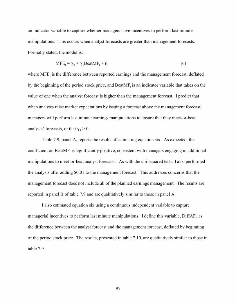
97

an indicator variable to capture whether managers have incentives to perform last minute

manipulations. This occurs when analyst forecasts are greater than management forecasts.

Formally stated, the model is:

MFEt = (0 + (1BeatMFt + 0t (6)

where MFEt is the difference between reported earnings and the management forecast, deflated

by the beginning of the period stock price, and BeatMFt is an indicator variable that takes on the

value of one when the analyst forecast is higher than the management forecast. I predict that

when analysts raise market expectations by issuing a forecast above the management forecast,

managers will perform last minute earnings manipulations to ensure that they meet-or-beat

analysts’ forecasts, or that (1 > 0.

Table 7.9, panel A, reports the results of estimating equation six. As expected, the

coefficient on BeatMFt is significantly positive, consistent with managers engaging in additional

manipulations to meet-or-beat analyst forecasts. As with the chi-squared tests, I also performed

the analysis after adding $0.01 to the management forecast. This addresses concerns that the

management forecast does not include all of the planned earnings management. The results are

reported in panel B of table 7.9 and are qualitatively similar to those in panel A.

I also estimated equation six using a continuous independent variable to capture

managerial incentives to perform last minute manipulations. I define this variable, DiffAFt, as

the difference between the analyst forecast and the management forecast, deflated by beginning

of the period stock price. The results, presented in table 7.10, are qualitatively similar to those in

table 7.9.

98

7.7 Conclusions

The evidence in this chapter suggests that asymmetries in the analyst forecast error

distribution are caused by managers’ last minute earnings manipulations. This reconciles the

asymmetries identified by Abarbanell and Lehavy (2003) with my findings that analysts include

earnings management in their forecast. Assuming that last minute manipulations follow the same

pattern as other earnings manipulations, the evidence also suggests that the difference between

management forecasts and earnings announcements might be a useful proxy for earnings

management.

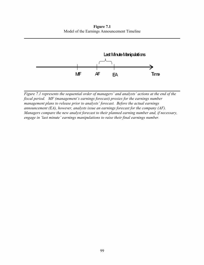
99

Figure 7.1Model of the Earnings Announcement Timeline

Figure 7.1 represents the sequential order of managers’ and analysts’ actions at the end of thefiscal period. MF (management’s earnings forecast) proxies for the earnings numbermanagement plans to release prior to analysts’ forecast. Before the actual earningsannouncement (EA), however, analysts issue an earnings forecast for the company (AF). Managers compare the new analyst forecast to their planned earning number and, if necessary,engage in ‘last minute’ earnings manipulations to raise their final earnings number.

100

Table 7.1Sample Selection Criteria for the Sample of Management Forecasts

Table 7.1 summarizes the sample selection procedure used to create a sample of managementforecasts used to for last minute manipulations. The initial sample consists of all annual pointand range management forecasts from 1985-2004. Observations made outside of the 20 daywindow prior to the end of the fiscal period or missing the necessary analyst forecast orbeginning of the period stock price data are then removed.

Initial sample of annual, earnings per share, point and range forecasts from 1985-2004 23,927 Less:

Observations not made within the 20 days prior to the period end (23,406)Observations missing analyst or beginning of the period priceinformation (209)

Management forecast sample 312

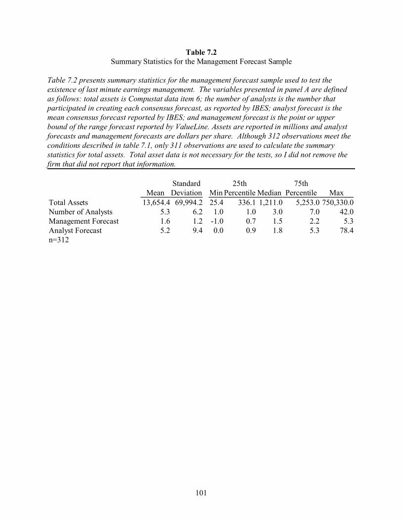
101

Table 7.2Summary Statistics for the Management Forecast Sample

Table 7.2 presents summary statistics for the management forecast sample used to test theexistence of last minute earnings management. The variables presented in panel A are definedas follows: total assets is Compustat data item 6; the number of analysts is the number thatparticipated in creating each consensus forecast, as reported by IBES; analyst forecast is themean consensus forecast reported by IBES; and management forecast is the point or upperbound of the range forecast reported by ValueLine. Assets are reported in millions and analystforecasts and management forecasts are dollars per share. Although 312 observations meet theconditions described in table 7.1, only 311 observations are used to calculate the summarystatistics for total assets. Total asset data is not necessary for the tests, so I did not remove thefirm that did not report that information.

Standard 25th 75thMean Deviation Min Percentile Median Percentile Max

Total Assets 13,654.4 69,994.2 25.4 336.1 1,211.0 5,253.0 750,330.0Number of Analysts 5.3 6.2 1.0 1.0 3.0 7.0 42.0Management Forecast 1.6 1.2 -1.0 0.7 1.5 2.2 5.3Analyst Forecast 5.2 9.4 0.0 0.9 1.8 5.3 78.4n=312

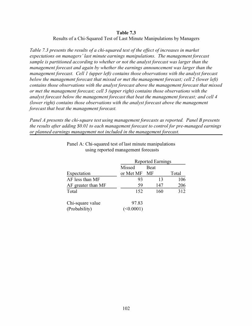
102

Table 7.3Results of a Chi-Squared Test of Last Minute Manipulations by Managers

Table 7.3 presents the results of a chi-squared test of the effect of increases in marketexpectations on managers’ last minute earnings manipulations. The management forecastsample is partitioned according to whether or not the analyst forecast was larger than themanagement forecast and again by whether the earnings announcement was larger than themanagement forecast. Cell 1 (upper left) contains those observations with the analyst forecastbelow the management forecast that missed or met the management forecast; cell 2 (lower left)contains those observations with the analyst forecast above the management forecast that missedor met the management forecast; cell 3 (upper right) contains those observations with theanalyst forecast below the management forecast that beat the management forecast; and cell 4(lower right) contains those observations with the analyst forecast above the managementforecast that beat the management forecast.

Panel A presents the chi-square test using management forecasts as reported. Panel B presentsthe results after adding $0.01 to each management forecast to control for pre-managed earningsor planned earnings management not included in the management forecast.

Panel A: Chi-squared test of last minute manipulations using reported management forecasts

Reported EarningsMissed Beat

Expectation or Met MF MF TotalAF less than MF 93 13 106AF greater than MF 59 147 206Total 152 160 312

Chi-square value 97.83(Probability) (<0.0001)

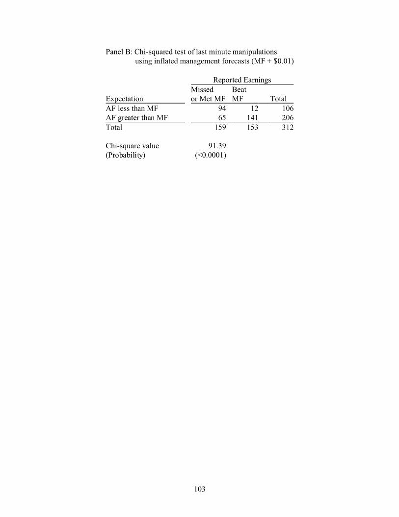
103

Panel B: Chi-squared test of last minute manipulations using inflated management forecasts (MF + $0.01)

Reported EarningsMissed Beat

Expectation or Met MF MF TotalAF less than MF 94 12 106AF greater than MF 65 141 206Total 159 153 312

Chi-square value 91.39(Probability) (<0.0001)

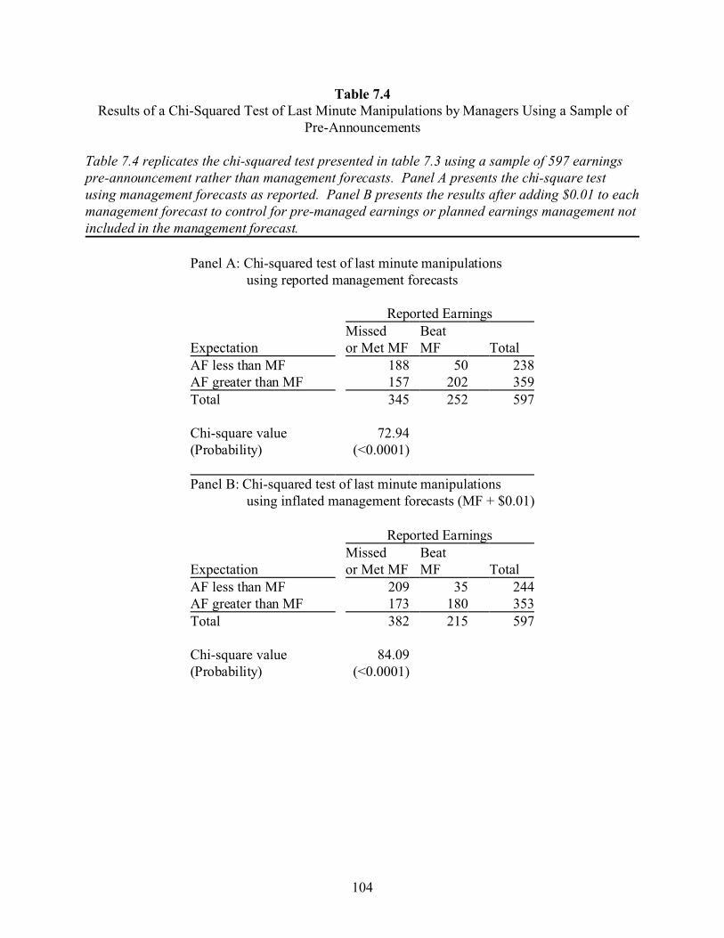
104

Table 7.4Results of a Chi-Squared Test of Last Minute Manipulations by Managers Using a Sample of

Pre-Announcements

Table 7.4 replicates the chi-squared test presented in table 7.3 using a sample of 597 earningspre-announcement rather than management forecasts. Panel A presents the chi-square testusing management forecasts as reported. Panel B presents the results after adding $0.01 to eachmanagement forecast to control for pre-managed earnings or planned earnings management notincluded in the management forecast.

Panel A: Chi-squared test of last minute manipulations using reported management forecasts

Reported EarningsMissed Beat

Expectation or Met MF MF TotalAF less than MF 188 50 238AF greater than MF 157 202 359Total 345 252 597

Chi-square value 72.94(Probability) (<0.0001) Panel B: Chi-squared test of last minute manipulations

using inflated management forecasts (MF + $0.01)

Reported EarningsMissed Beat

Expectation or Met MF MF TotalAF less than MF 209 35 244AF greater than MF 173 180 353Total 382 215 597

Chi-square value 84.09(Probability) (<0.0001)

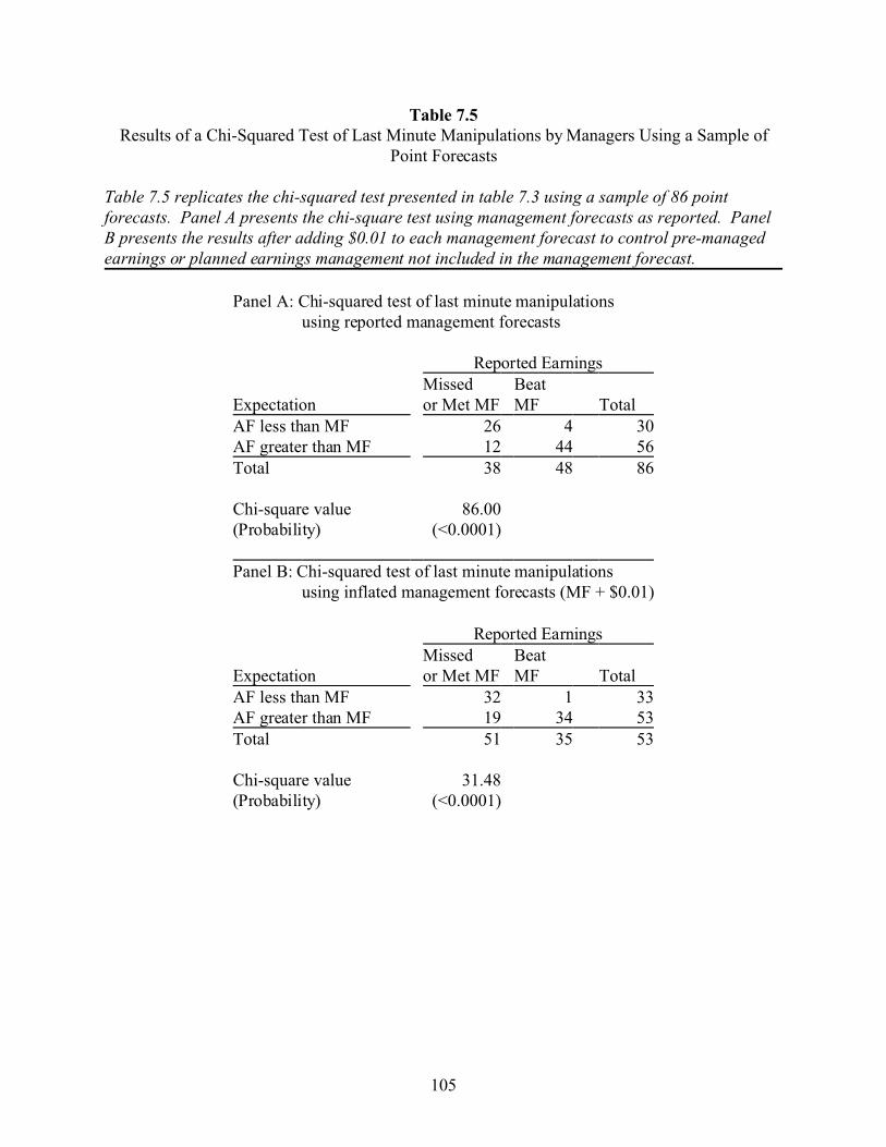
105

Table 7.5Results of a Chi-Squared Test of Last Minute Manipulations by Managers Using a Sample of

Point Forecasts

Table 7.5 replicates the chi-squared test presented in table 7.3 using a sample of 86 pointforecasts. Panel A presents the chi-square test using management forecasts as reported. PanelB presents the results after adding $0.01 to each management forecast to control pre-managedearnings or planned earnings management not included in the management forecast.

Panel A: Chi-squared test of last minute manipulations using reported management forecasts

Reported EarningsMissed Beat

Expectation or Met MF MF TotalAF less than MF 26 4 30AF greater than MF 12 44 56Total 38 48 86

Chi-square value 86.00(Probability) (<0.0001) Panel B: Chi-squared test of last minute manipulations

using inflated management forecasts (MF + $0.01)

Reported EarningsMissed Beat

Expectation or Met MF MF TotalAF less than MF 32 1 33AF greater than MF 19 34 53Total 51 35 53

Chi-square value 31.48(Probability) (<0.0001)

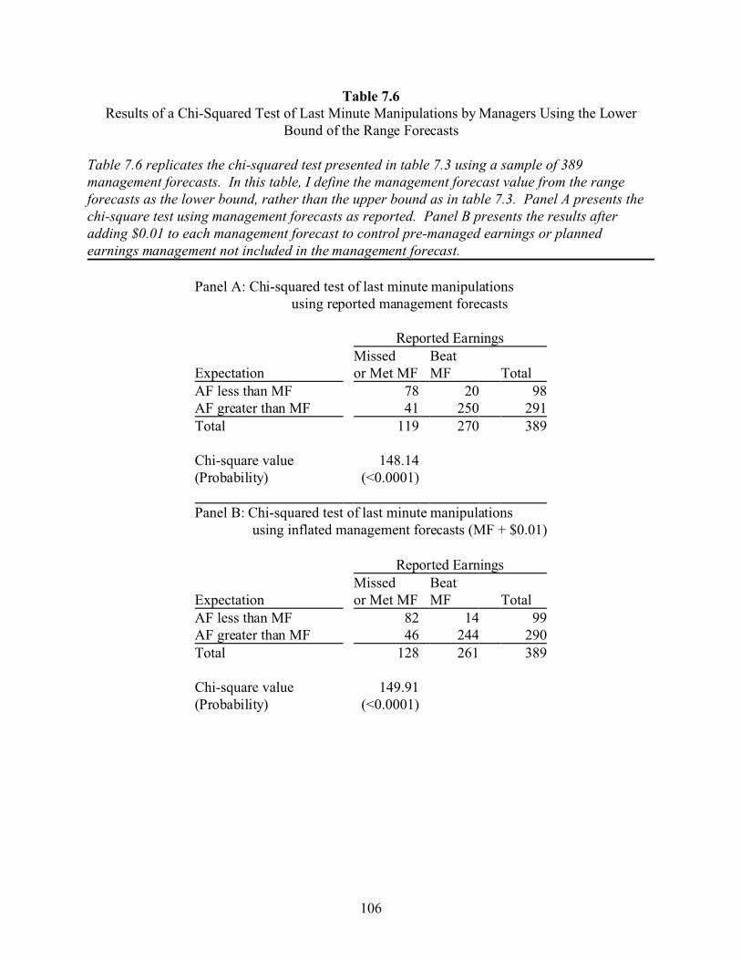
106

Table 7.6Results of a Chi-Squared Test of Last Minute Manipulations by Managers Using the Lower

Bound of the Range Forecasts

Table 7.6 replicates the chi-squared test presented in table 7.3 using a sample of 389management forecasts. In this table, I define the management forecast value from the rangeforecasts as the lower bound, rather than the upper bound as in table 7.3. Panel A presents thechi-square test using management forecasts as reported. Panel B presents the results afteradding $0.01 to each management forecast to control pre-managed earnings or plannedearnings management not included in the management forecast.

Panel A: Chi-squared test of last minute manipulations using reported management forecasts

Reported EarningsMissed Beat

Expectation or Met MF MF TotalAF less than MF 78 20 98AF greater than MF 41 250 291Total 119 270 389

Chi-square value 148.14(Probability) (<0.0001) Panel B: Chi-squared test of last minute manipulations

using inflated management forecasts (MF + $0.01)

Reported EarningsMissed Beat

Expectation or Met MF MF TotalAF less than MF 82 14 99AF greater than MF 46 244 290Total 128 261 389

Chi-square value 149.91(Probability) (<0.0001)

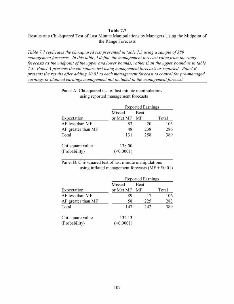
107

Table 7.7Results of a Chi-Squared Test of Last Minute Manipulations by Managers Using the Midpoint of

the Range Forecasts

Table 7.7 replicates the chi-squared test presented in table 7.3 using a sample of 389management forecasts. In this table, I define the management forecast value from the rangeforecasts as the midpoint of the upper and lower bounds, rather than the upper bound as in table7.3. Panel A presents the chi-square test using management forecasts as reported. Panel Bpresents the results after adding $0.01 to each management forecast to control for pre-managedearnings or planned earnings management not included in the management forecast.

Panel A: Chi-squared test of last minute manipulations using reported management forecasts

Reported EarningsMissed Beat

Expectation or Met MF MF TotalAF less than MF 83 20 103AF greater than MF 48 238 286Total 131 258 389

Chi-square value 138.00(Probability) (<0.0001) Panel B: Chi-squared test of last minute manipulations

using inflated management forecasts (MF + $0.01)

Reported EarningsMissed Beat

Expectation or Met MF MF TotalAF less than MF 89 17 106AF greater than MF 58 225 283Total 147 242 389

Chi-square value 132.13(Probability) (<0.0001)

108

Table 7.8Results of a Chi-Squared Test of Last Minute Manipulations by Managers After Removing 2001

and 2002

Table 7.8 replicates the chi-squared test presented in table 7.3 after removing the observationsfrom 2001 and 2002. The resulting sample consists of 247 management forecasts. Panel Apresents the chi-square test using management forecasts as reported. Panel B presents theresults after adding $0.01 to each management forecast to control for pre-managed earnings orplanned earnings management not included in the management forecast.

Panel A: Chi-squared test of last minute manipulations using reported management forecasts

Reported EarningsMissed Beat

Expectation or Met MF MF TotalAF less than MF 63 10 73AF greater than MF 46 128 174Total 109 138 247

Chi-square value 74.75(Probability) (<0.0001) Panel B: Chi-squared test of last minute manipulations

using inflated management forecasts (MF + $0.01)

Reported EarningsMissed Beat

Expectation or Met MF MF TotalAF less than MF 64 9 73AF greater than MF 51 123 174Total 115 132 247

Chi-square value 70.39(Probability) (<0.0001)

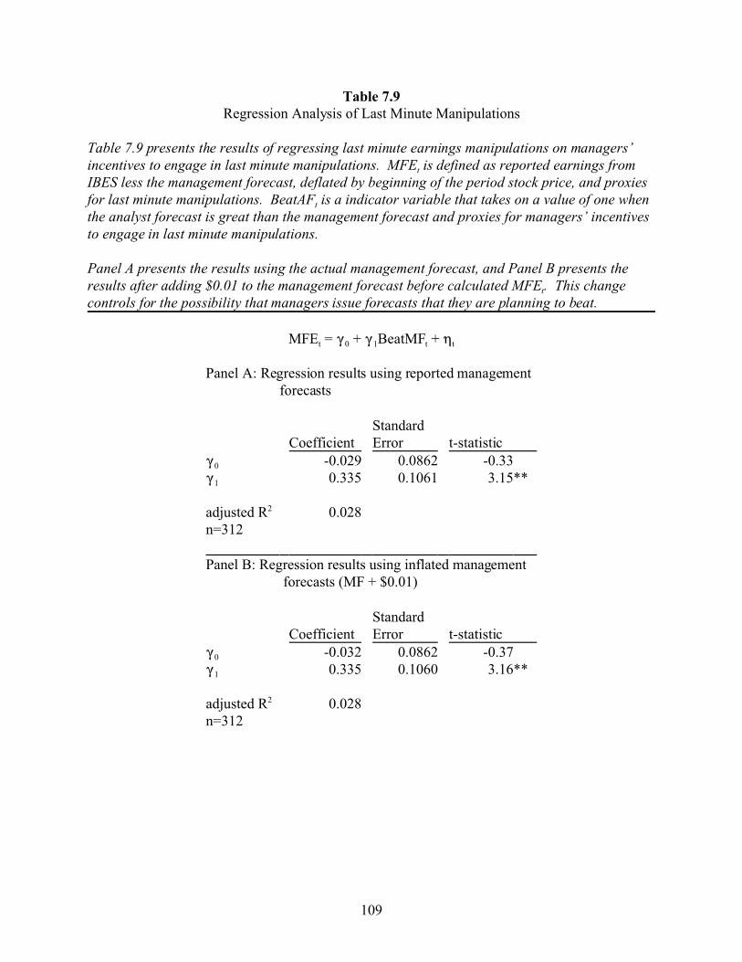
109

Table 7.9Regression Analysis of Last Minute Manipulations

Table 7.9 presents the results of regressing last minute earnings manipulations on managers’incentives to engage in last minute manipulations. MFEt is defined as reported earnings fromIBES less the management forecast, deflated by beginning of the period stock price, and proxiesfor last minute manipulations. BeatAFt is a indicator variable that takes on a value of one whenthe analyst forecast is great than the management forecast and proxies for managers’ incentivesto engage in last minute manipulations.

Panel A presents the results using the actual management forecast, and Panel B presents theresults after adding $0.01 to the management forecast before calculated MFEt. This changecontrols for the possibility that managers issue forecasts that they are planning to beat.

MFEt = (0 + (1BeatMFt + 0t

Panel A: Regression results using reported management forecasts

CoefficientStandardError t-statistic

(0 -0.029 0.0862 -0.33(1 0.335 0.1061 3.15**

adjusted R2 0.028n=312 Panel B: Regression results using inflated management

forecasts (MF + $0.01)

CoefficientStandardError t-statistic

(0 -0.032 0.0862 -0.37(1 0.335 0.1060 3.16**

adjusted R2 0.028n=312

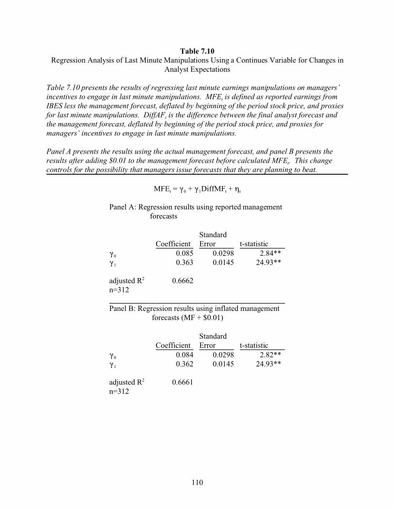
110

Table 7.10Regression Analysis of Last Minute Manipulations Using a Continues Variable for Changes in

Analyst Expectations

Table 7.10 presents the results of regressing last minute earnings manipulations on managers’incentives to engage in last minute manipulations. MFEt is defined as reported earnings fromIBES less the management forecast, deflated by beginning of the period stock price, and proxiesfor last minute manipulations. DiffAFt is the difference between the final analyst forecast andthe management forecast, deflated by beginning of the period stock price, and proxies formanagers’ incentives to engage in last minute manipulations.

Panel A presents the results using the actual management forecast, and panel B presents theresults after adding $0.01 to the management forecast before calculated MFEt. This changecontrols for the possibility that managers issue forecasts that they are planning to beat.

MFEt = (0 + (1DiffMFt + 0t

Panel A: Regression results using reported management forecasts

CoefficientStandardError t-statistic

(0 0.085 0.0298 2.84**(1 0.363 0.0145 24.93**

adjusted R2 0.6662n=312 Panel B: Regression results using inflated management

forecasts (MF + $0.01)

CoefficientStandardError t-statistic

(0 0.084 0.0298 2.82**(1 0.362 0.0145 24.93**

adjusted R2 0.6661n=312

111

CHAPTER 8

CONCLUSION

8.1 Summary

Recent studies by Abarbanell and Lehavy (2003) and Burgstahler and Eames (2003)

produce conflicting implications regarding how analysts incorporate earnings management into

their forecasts. Burgstahler and Eames (2003) suggest that analysts include the effects of

earnings management in order to more accurately forecast reported earnings, while Abarbanell

and Lehavy (2003) argue that analysts remove the effects of earnings management in order to

forecast pre-managed earnings. The purpose of this dissertation has been to determine which of

these findings is supported by the data.

Using a model similar to that used by Elgers et al. (2003), I tested the predictive value of

current discretionary accruals on upcoming earnings and the weight analysts place on

discretionary accruals when forecasting upcoming earnings. The evidence suggests that analysts

include the information in discretionary accruals (a proxy for earnings management) when

forecasting upcoming earnings. In addition, I examined the association between analyst forecasts

and reported and restated earnings. Using a Vuong test, I found evidence that analyst forecasts

are more highly associated with reported than with restated earnings. This is also consistent with

analysts including the effects of earnings management in their forecasts.

Although these tests support the findings of Burgstahler and Eames (2003), they do not

explain the asymmetries in the analyst forecast error distribution documented by Abarbanell and

Lehavy (2003). Brown (1998) suggests that these asymmetries are caused by last minute

112

manipulations by managers, rather than by analysts intentionally removing the effects of earnings

managements. My results support this view. This reconciles the results of Abarbanell and

Lehavy (2003) and Burgstahler and Eames (2003).

8.2 Implications for Future Research

If analysts include the effects of earnings management in their forecasts, and investors

accept their forecast as an accurate prediction of a company’s performance, then earnings

management becomes a self-fulfilling prophecy as managers scramble to make the forecast.

Additional research is needed to determine how investors price the earnings manipulations

included in analysts’ forecasts and to what extent their pricing is rational. Additional research

could also address whether the evidence of analyst bias observed in prior studies (Kadous et al.

2004) is due to the use of reported earnings, instead of earnings before last minute manipulations,

as the benchmark for analyst performance. Finally, to the extent that the difference between

management forecasts and earnings announcement is an accurate proxy for last minute earnings

manipulations, it could be useful to researchers studying earnings management.

8.3 Limitations

My results are subject to four major caveats. First, the tests are based on several

assumptions that may not be completely descriptive. Of particular concern is the assumption that

analysts provide all of their information to investors through their earnings forecast. While this

assumption is consistent with the prior literature, it is possible that analysts convey their

information regarding earnings management in the body of their report, in their stock

113

recommendation, in another forecast, or in some other manner. If so, then analysts have little, if

any, incentive to remove earnings management from their earnings forecast.

The second caveat concerns variable measurement. Earnings management, pre-managed

earnings, and the level of earnings prior to last minute manipulations are all unobservable. Thus,

any proxy variable is subject to considerable noise. It is possible that the results are due to this

noise rather than to the hypothesized relationships. Similarly, the results of the Vuong test are

limited by the possibility that the earnings restatements are due to reasons other than earnings

management.

A third concern is the generalizability of the results. In particular, the management

forecast sample used to test the last minute manipulations explanation for the asymmetries in the

analyst forecast error distribution may not be representative of the broader population of firms.

Sample screens reduced the usable observations for this analysis from 23,927 to only 312.

Although the voluntary disclosure literature has traditionally used smaller samples, it is possible

that the results presented in chapter 7 will not hold for a wider selection of firms.

A final caveat is that the tests are exclusively based on archival data taken from the IBES,

FirstCall, Compustat, and CRSP databases. Although this data provides an overall picture of

analysts and their forecasts, information obtained from actual analysts in a survey or

experimental setting might be useful for addressing the research hypotheses from another

perspective. I leave such a test to future research.

114

REFERENCES

Abarbanell, J. and V. Bernard. "Is the U.S. Stock Market Myopic?" Journal of AccountingResearch (2000): 221-242.

Abarbanell, J. and R. Lehavy. "Biased forecasts or biased earnings? The role of reported earningsin explaining apparent bias and over/underreaction in analysts' earnings forecasts."Journal of Accounting and Economics (2003): 105-146.

Abarbanell, J. S. "Do analysts' earnings forecasts incorporate information in prior stock pricechanges?" Journal of Accounting & Economics (1991): 147-165.

Abdel-Khalik, A. R. and J. Espejo. "Expectations Data and the Predictive Value of InterimReporting." Journal of Accounting Research (1978): 1-13.

Arya, A.; J. C. Glover and S. Sunder. "Are Unmanaged Earnings Always Better forShareholders?" Accounting Horizons (2003): 111-116.

Ayers, B. C.; J. X. Jiang and P. E. Yeung. "Discretionary Accruals and Earnings Management:An Analysis of Pseudo Earnings Targets." Accounting Review (2006): 617-652.

Baginski, S.; J. Hassell and G. Waymire. "Some Evidence on the News Content of PreliminaryEarnings Estimates." Accounting Review (1994): 265-271.

Balsam, S.; E. Bartov and C. Marquardt. "Accruals Management, Investor Sophistication, andEquity Valuation: Evidence from 10Q Filings." Journal of Accounting Research (2002):987-1012.

Bamber, L. S. and Y. S. Cheon. "Discretionary management earnings forecast disclosures:Antecedents and outcomes associated with Forecast Venue and Forecast SpecificityChoices." Journal of Accounting Research (1998): 167-190.

Barron, O. E.; D. Byard; C. Kile and E. J. Riedl. "High-Technology Intangibles and Analysts'Forecasts." Journal of Accounting Research (2002): 289-312.

Barron, O. E.; D. Byard and O. Kim. "Changes in Analysts' Information around EarningsAnnouncements." Accounting Review (2002): 821-846.

Barron, O. E.; O. Kim; S. C. Lim and D. E. Stevens. "Using analysts' forecasts to measureproperties of analysts' information environment." Accounting Review (1998): 421-433.

115

Barth, M. E.; R. Kasznik and M. F. McNichols. "Analyst Coverage and Intangible Assets."Journal of Accounting Research (2001): 1-34.

Barton, J. and P. J. Simko. "The Balance Sheet as an Earnings Management Constraint."Accounting Review (2002): 1-27.

Bartov, E.; D. Givoly and C. Hayn. "The rewards to meeting or beating earnings expectations."Journal of Accounting and Economics (2002): 173-204.

Bartov, E.; F. A. Gul and J. S. L. Tsui. "Discretionary-accruals models and audit qualifications."Journal of Accounting and Economics (2001): 421-452.

Beneish, M. D. and M. E. Vargus. "Insider Trading, Earnings Quality, and Accrual Mispricing."Accounting Review (2002): 755-791.

Bernard, V. L. "Cross-Sectional Dependence and Problems in Inference in Market-BasedAccounting Research." Journal of Accounting Research (1987): 1-48.

Bradshaw, M. T. "How Do Analysts Use Their Earnings Forecasts in Generating StockRecommendations?" (December, 2004). Available at SSRN:http://ssrn.com/abstract=256438.

Bradshaw, M. T. and L. D. Brown. "Do Sell-Side Analysts Exhibit Differential Target PriceForecasting Ability?" (April 15, 2006). Available at SSRN:http://ssrn.com/abstract=698581.

Bradshaw, M. T.; S. A. Richardson and R. G. Sloan. "Do Analysts and Auditors Use Informationin Accruals?" Journal of Accounting Research (2001): 45-74.

Bradshaw, M. T. and R. G. Sloan. "GAAP versus The Street: An Empirical Assessment of TwoAlternative Definitions of Earnings." Journal of Accounting Research (2002): 41-66.

Brown, L. D. "Analyst Forecasting Errors: Additional Evidence." Financial Analysts Journal(1997): 81-88.

Brown, L. D. "Earnings forecasting research: its implications for capital markets research."International Journal of Forecasting (1993): 295-320.

Brown, L. D. "Managerial Behavior and the Bias in Analysts' Earnings Forecasts." (July 2, 1998).Available at SSRN: http://ssrn.com/abstract=113508.

Brown, L. D. and M. L. Caylor. "A Temporal Analysis of Quarterly Earnings Thresholds:Propensities and Valuation Consequences." Accounting Review (2005): 423-440.

Brown, L. D. and J. C. Y. Han. "The impact of annual earnings announcements on convergenceof beliefs." Accounting Review (1992): 862-875.

116

Brown, L. D. and M. S. Rozeff. "The Superiority of Analyst Forecasts as Measures ofExpectations: Evidence from Earnings." Journal of Finance (1978): 1-16.

Burgstahler, D. and I. Dichev. "Earnings management to avoid earnings decreases and losses."Journal of Accounting and Economics (1997): 99-126.

Burgstahler, D. C. and M. J. Eames. "Earnings Management to Avoid Losses and EarningsDecreases: Are Analysts Fooled?" Contemporary Accounting Research (2003): 253-294.

Chandar, N. and R. Bricker. "Incentives, Discretion, and Asset Valuation in Closed End MutualFunds." Journal of Accounting Research (2002): 1037-1070.

Clement, M. "Analyst forecast accuracy: Do ability, resources, and portfolio complexity matter?"Journal of Accounting and Economics (1999): 285-303.

Crichfield, T.; T. Dyckman and J. Lakonishok. "An Evaluation of Security Analysts' Forecasts."Accounting Review (1978): 651-668.

Das, S.; C. B. Levine and K. Sivaramakrishnan. "Earnings predictability and bias in analysts'earnings forecasts." Accounting Review (1998): 277-294.

Dechow, P. M. "Accounting earnings and cash flows as measures of firm performance : The roleof accounting accruals." Journal of Accounting and Economics (1994): 3-42.

DeFond, M. L. and C. W. Park. "Smoothing income in anticipation of future earnings." Journalof Accounting and Economics (1997): 115-139.

Degeorge, F.; J. Patel and R. Zeckhauser. "Earnings Management to Exceed Thresholds."Journal of Business (1999): 1-33.

Dhaliwal, D.; C. A. Gleason and L. F. Mills. "Last Chance Earnings Management: Using the TaxExpense to Achieve Earnings Targets." (June, 2003). Available at SSRN:http://ssrn.com/abstract=314563.

Dichev, I. D. and D. J. Skinner. "Large Sample Evidence on the Debt Covenant Hypothesis."Journal of Accounting Research (2002): 1091-1123.

Durtschi, C. and P. Easton. "Earnings Management? The Shapes of the Frequency Distributionsof Earnings Metrics Are Not Evidence Ipso Facto." Journal of Accounting Research(2005): 557-592.

Elgers, P. T.; M. H. Lo and J. Pfeiffer, Ray J. "Analysts' vs. investors' weightings of accruals inforecasting annual earnings." Journal of Accounting and Public Policy (2003): 255-280.

Elgers, P. T.; M. H. Lo and R. J. Pfeiffer Jr. "Delayed Security Price Adjustments to FinancialAnalysts' Forecasts of Annual Earnings." Accounting Review (2001): 613-632.

117

Enis, C. R. and B. Ke. "The Impact of the 1986 Tax Reform Act on Income Shifting fromCorporate to Shareholder Tax Bases: Evidence from the Motor Carrier Industry." Journalof Accounting Research (2003): 65-88.

Erickson, M.; M. Hanlon and E. L. Maydew. "How Much Will Firms Pay for Earnings That DoNot Exist? Evidence of Taxes Paid on Allegedly Fraudulent Earnings." AccountingReview (2004): 387-408.

Fischer, P. E. and R. E. Verrecchia. "Reporting Bias." Accounting Review (2000): 229-245.

Frankel, R. and C. M. C. Lee. "Accounting valuation, market expectation, and cross-sectionalstock returns." Journal of Accounting and Economics (1998): 283-319.

Gaver, J. J.; K. M. Gaver and J. R. Austin. "Additional evidence on bonus plans and incomemanagement." Journal of Accounting and Economics (1995): 3-28.

Gaver, J. J. and J. S. Paterson. "Do insurers manipulate loss reserves to mask solvencyproblems?" Journal of Accounting and Economics (2004): 393-416.

Gigler, F. B. and T. Hemmer. "Conservatism, Optimal Disclosure Policy, and the Timeliness ofFinancial Reports." Accounting Review (2001): 471-493.

Gintschel, A. and S. Markov. "The effectiveness of Regulation FD." Journal of Accounting andEconomics (2004): 293-314.

Guidry, F.; A. J. Leone and S. Rock. "Earnings-based bonus plans and earnings management bybusiness-unit managers." Journal of Accounting and Economics (1999): 113-142.

Healy, P. M. "The effect of bonus schemes on accounting decisions." Journal of Accounting andEconomics (1985): 85-107.

Herrmann, D.; T. Inoue and W. B. Thomas. "The Sale of Assets to Manage Earnings in Japan."Journal of Accounting Research (2003): 89-108.

Hope, O.-K. "Disclosure Practices, Enforcement of Accounting Standards, and Analysts' ForecastAccuracy: An International Study." Journal of Accounting Research (2003): 235-272.

Hribar, P. and D. W. Collins. "Errors in Estimating Accruals: Implications for EmpiricalResearch." Journal of Accounting Research (2002): 105-134.

Huang, A. H.; R. H. Willis and A. Y. Zhang. "Bold Security Analysts' Earnings Forecasts andManagers' Information Flow." (January, 2005). Available at SSRN:http://ssrn.com/abstract=587951.

Irvine, P. "Do analysts generate trade for their firms? Evidence from the Toronto stockexchange." Journal of Accounting and Economics (2000): 209-226.

118

Irvine, P. J. "Analysts' Forecasts and Brokerage-Firm Trading." Accounting Review (2004): 125-149.

Jacob, J.; T. Z. Lys and M. A. Neale. "Expertise in forecasting performance of security analysts."Journal of Accounting & Economics (1999): 51-82.

Jones, J. J. "Earnings Management During Import Relief Investigations." Journal of AccountingResearch (1991): 193-228.

Jones, K.; G. V. Krishnan and K. Melendez. "Do Models of Discretionary Accruals DetectActual Cases of Fraudulent and Restated Earnings? An Empirical Evaluation." (April 6,2006). Available at SSRN: http://ssrn.com/abstract=895541.

Kadous, K.; S. D. Kirsche and L. M. Sedor. "Using Counter-explanation to Limit UnintentionalOptimism in Analysts' Forecasts." (October, 2004). Available at SSRN:http://ssrn.com/abstract=623042.

Kasznik, R. "On the association between voluntary disclosure and earnings management."(1999///Spring, 1999). Available at SSRN:http://search.epnet.com/login.aspx?direct=true&db=buh&an=2205751.

Ke, B.; S. Huddart and K. Petroni. "What insiders know about future earnings and how they useit: Evidence from insider trades." Journal of Accounting and Economics (2003): 315-346.

Kim, K. and D. A. Schroeder. "Analysts' use of managerial bonus incentives in forecastingearnings." Journal of Accounting and Economics (1990): 4-23.

Kim, O.; S. C. Lim and K. W. Shaw. "The Inefficiency of the Mean Analyst Forecast as aSummary Forecast of Earnings." Journal of Accounting Research (2001): 329-335.

Kim, O. and R. E. Verrecchia. "Market liquidity and volume around earnings announcements."Journal of Accounting and Economics (1994): 41-67.

Kothari, S. P. "Capital markets research in accounting." Journal of Accounting and Economics(2001): 105-231.

Kothari, S. P.; A. J. Leone and C. E. Wasley. "Performance matched discretionary accrualmeasures." Journal of Accounting and Economics (2005): 163-197.

Lang, M. H.; K. V. Lins and D. P. Miller. "Concentrated Control, Analyst Following, andValuation: Do Analysts Matter Most When Investors Are Protected Least?" Journal ofAccounting Research (2004): 589-623.

Leone, A. J. and J. S. Wu. "What Does it Take to Become a Superstar? Evidence fromInstitutional Investor Rankings of Financial Analysts." (May, 2002). Available at SSRN:http://papers.ssrn.com/sol3/papers.cfm?abstract_id=313594.

119

Liu, X. "Analysts' Response to Earnings Management." (March 1, 2005). Available at SSRN:http://ssrn.com/abstract=622404.

Matsumoto, D. A. "Management's Incentives to Avoid Negative Earnings Surprises." AccountingReview (2002): 483-514.

McVay, S. E.; V. Nagar and W. V. Tang. "Trading Incentives to Meet Earnings Thresholds."(April, 2006). Available at SSRN: http://ssrn.com/abstract=555202.

Mikhail, M. B.; B. R. Walther and R. H. Willis. "Does Forecast Accuracy Matter to SecurityAnalysts?" Accounting Review (1999): 185-200.

Mikhail, M. B.; B. R. Walther and R. H. Willis. "The effect of experience on security analystunderreaction." Journal of Accounting & Economics (2003): 101-116.

Mikhail, M. B.; B. R. Walther and R. H. Willis. "Security Analyst Experience and Post-Earnings-Announcement Drift." Journal of Accounting, Auditing & Finance (2003): 529-555.

Morse, D. and J. Stephan. "Earnings announcements and the convergence (or divergence) ofbeliefs." Accounting Review (1991): 376-388.

Palmrose, Z.-V.; V. J. Richardson and S. Scholz. "Determinants of market reactions torestatement announcements." Journal of Accounting and Economics (2004): 59-89.

Payne, J. L. and W. B. Thomas. "The Implications of Using Stock-Split Adjusted I/B/E/S Data inEmpirical Research." Accounting Review (2003): 1049-1067.

Pinello, A. S. "How Do Individual Investors Use Analyst Forecasts? The Implications forInvestor Reaction to Forecast Revisions and Earnings Surprises." (November 15, 2005).Available at SSRN: http://ssrn.com/abstract=817006.

Plumlee, M. A. "The Effect of Information Complexity on Analysts' Use of That Information."Accounting Review (2003): 275-296.

Pownall, G. and G. Waymire. "Voluntary Disclosure Choice and Earnings Information Transfer."Journal of Accounting Research (1989): 85-105.

Ramnath, S. "Investor and Analyst Reactions to Earnings Announcements of Related Firms: AnEmpirical Analysis." Journal of Accounting Research (2002): 1351-1376.

Schipper, K. "Analysts' forecasts." Accounting Horizons (1991): 105-121.

Schipper, K. "Commentary on Earnings Management." Accounting Horizons (1989): 91-102.

120

Shane, P. and P. Brous. "Investor and (Value Line) Analyst Underreaction to Information aboutFuture Earnings: The Corrective Role of Non-Earnings-Surprise Information." Journal ofAccounting Research (2001): 387-404.

Skinner, D. J. "Why firms voluntarily disclose bad news." Journal of Accounting Research(1994): 38-60.

Sloan, R. G. "Do Stock Prices Fully Reflect Information in Accruals and Cash Flows AboutFuture Earnings?" Accounting Review (1996): 289-315.

Soffer, L. C.; S. R. Thiagarajan and B. R. Walther. "Earnings Preannouncement Strategies."Review of Accounting Studies (2000): 5-26.

Stickel, S. E. "Reputation and Performance Among Security Analysts." Journal of Finance(1992): 1811-1836.

Subramanyam, K. R. "The pricing of discretionary accruals." Journal of Accounting andEconomics (1996): 249-281.

Tan, H.-T.; R. Libby and J. E. Hunton. "Analysts Reactions to Earnings PreannouncementStrategies." Journal of Accounting Research (2002): 223-246.

Tucker. "Does Disclosure Reputation Explain Earnings Warnings?" (August, 2004). Available atSSRN: http://ssrn.com/abstract=586211.

Vuong, Q. H. "Likelihood Ratio Tests for Model Selection and Non-Nested Hypotheses."Econometrica (1989): 307-333.

Waymire, G. "Additional Evidence on the Information Content of Management EarningsForecasts." Journal of Accounting Research (1984): 703-718.

Weber, D. P. "Book - Tax Differences, Analysts' Forecast Errors, and Stock Returns." WorkingPaper (2005).

Xie, H. "The Mispricing of Abnormal Accruals." Accounting Review (2001): 357-373.