Divided Landscapes of Economic Opportunity:The Canadian Geography of Intergenerational

Income MobilityMiles Corak∗

University of Ottawa

June 2017

Abstract

Intergenerational income mobility varies significantly across Canada, with the landscapeclustering into four broad regions. These are not geographically contiguous, andprovincial boundaries are not the dividing lines. The important exception is Manitoba,which has noticeably less intergenerational mobility among eight indicators derivedfrom a large administrative data set for a cohort of men and women born between 1963and 1970. These indicators are derived for each of the 266 Census Divisions in the1986 Canadian Census. They show that higher mobility communities are located inSouthwestern Ontario, Alberta, and Saskatchewan, and tend to be correlated withlower poverty, less income inequality, and a higher share of immigrants.

KEYWORDS: Intergenerational mobility, equality of opportunity, geographyJEL Classification: D63, J61, J62

∗I am professor of economics with the Graduate School of Public and International Affairs at the Universityof Ottawa, Ottawa Canada. The first draft of this paper was written while I was a visiting professor ofeconomics at Harvard University during the 2015/16 academic year. I am grateful to Yuri Ostrovsky for hishelp in updating the data and producing the statistics upon which my analysis is based. This was possible withthe cooperation of Statistics Canada through a cost recovery project, and the financial support of the SocialSciences and Humanities Research Council of Canada through Insight grant number 230936-191999-2001.Mary-Ellen Maybee and Brigit Levac of Statistics Canada kindly made Shapefiles associated with the 1986Census available, allowing me to map the data, which was done using R. I also thank Raj Chetty, NathanHendren, Branko Milanovic, Martin Nybom, and Jan Stuhler for their feedback on an earlier draft. Versionsof this paper have been presented at the April 2016 workshop on Inequalities and Families, organized by theResearch Group on Human Capital at the Université du Québec à Montréal; in May 2016 to the 41st Congressof the Association des Économistes Québecois held in Québec City, to the 15th Annual North AmericanBasic Income Guarantee Congress held in Winnipeg, and at the Northwestern University Global InequalityWorkshop in Evanston Illinois; in October 2016 to the Sixth Annual NYU/UCLA Tax Policy Symposium onTax Policy and Upward Mobility held at UCLA, Los Angeles California; in November 2016 as The ShoyamaLecture presented in Ottawa to the Department of Finance, Government of Canada; to the Canada Seminarat Harvard University in February 2017; to the Workshop on Interdisciplinary Approaches to Inequality andMobility held at Duke University in March 2017; to the 51st Annual Meetings of the Canadian EconomicsAssociation held at St Francis Xavier University, in Antigonish, Nova Scotia; and in departmental seminars atthe Graduate Center, City University of New York, the University of Ottawa, and the University of Waterloo.The statistics used in this paper, along with a host of supplementary information and data, as well as an onlineappendix examining the robustness of the findings, are available at MilesCorak.com/Equality-of-Opportunity.I can be reached at the same web site, and @MilesCorak. © Miles Corak, all rights reserved.

1

1 Introduction

“Equality of opportunity”—how likely it is, how it varies, and what causes it—is an importantissue in many rich countries. In part this is because of significant increases in income inequal-ity, and the now generally accepted view that higher inequality is associated with less socialmobility. Former US President Obama and his senior advisers have made reference to this(White House 2013; Krueger 2012; Furman 2016), as have important international organiza-tions like the International Monetary Fund, the Organization for Economic Cooperation andDevelopment, and Central Bankers like Janet Yellen (2014) of the US Federal Reserve andMark Carney (2014) of the Bank of England. This public policy attention warrants a certaincaution. “Equality of Opportunity” is a multifaceted concept that cannot be simply definedand measured, and while income mobility—the dimension most closely related to manypolicy discussions—may be an important aspect, it clearly is not the whole story. I offer ananalysis of only this dimension, the degree to which adult incomes are related to the incomesof the families in which children were raised, in other words the extent to which economicposition in one generation echoes into the next. Even with this focus, there are a host ofdifferent statistics used to describe the process. My main contribution to the understandingof intergenerational income dynamics in Canada is to offer estimates of mobility across spacein a way that pays attention to a broad suite of statistics capturing the many different waysacademic researchers, policy makers, and the general public view the process.

My primary objective is to estimate the degree of intergenerational income mobilitywithin each of hundreds of sub-provincial regions. The income tax forms Canadians submitto their governments is the information source, and offers very large sample sizes, in principlethe entire population upon which I focus, those born between 1963 and 1970. Up to nowthe advantages of these data have been exploited to very precisely measure the degreeof intergenerational mobility, to examine the process by income source, and to estimatehow it varies across the income distribution. All of this is for the country as a whole, yetthe large sample holds the potential for more detailed sub-national analysis. I use theseintergenerationally linked T1 forms to calculate and examine different dimensions of economicmobility for each of the 266 Census Divisions defined in the 1986 Canadian Census.

In this way I hope to paint a detailed picture of the extent to which adult outcomes arerelated to family background, and how the relationship varies across the country. Many ofthe factors and policies that theory suggests influence generational mobility vary significantlyacross space, or fall within the domain of provincial and municipal governments. Schooling,health care, employment opportunities for youth, and basic income support for familiesinvolve not just the federal government, but in a major way provincial legislatures and citycouncils. A sub-national portrait allows policy makers to know their own regions, and tomake comparisons with others. While the existing literature suggests that Canada is anintergenerationally mobile country, and in particular more mobile than the United States, anational focus potentially masks significant geographic variation within the country, and placesa blind spot over the experiences and needs of certain demographic groups and communities.

I use a suite of statistical measures that collectively offer a fuller picture of intergen-erational income mobility. This process cannot be summarized with one statistic, yet the

2

existing economics literature puts a great deal of emphasis on the intergenerational elasticity,the percentage difference in a child’s adult income for a one percentage point differencein parent income. This is a valuable relative measure of mobility that offers a summaryindicator of how income inequality evolves across generations. But it is not a completedescription of the process, nor does it relate to some policy-relevant ways of thinking aboutit. More specific measures are needed to speak to obvious concerns: to what extent doesthe current generation earn on average more or less than the previous generation, to whatextent are rank and relative position transmitted across generations, and to what extent arelow and top incomes transmitted intergenerationally? Income mobility, rank mobility, anddirectional mobility—particularly upward mobility from the bottom—all relate to aspects ofsocial welfare, and capture the political imagination.

I also fully account for the role and outcomes of women, an important gap in the existingliterature. Focusing on men—fathers and sons—might be a convenient simplification. If onlymen work in the market, then family income is the income of the father. If the participationrates of women are low and intermittent as a result of child care responsibilities fallingupon them, then their income is more easily approximated by the income of their partners.Focusing on adult sons makes the analysis easier by avoiding the need to model these otherdimensions. These assumptions skew our understanding of the intergenerational transmissionprocess, and they potentially put aside significant numbers of individuals, both men andwomen, raised by single mothers. My analysis is based on “family” income, defined as thetotal income of both partners, including periods when there is only one parent present. Theanalysis is conducted for sons and daughters without distinction.

I find that intergenerational income mobility varies significantly across the country witha significant fraction of children raised by low income parents facing considerable chancesof an intergenerational cycle of poverty, and limited opportunity of rising to the top. Atthe broadest level the Canadian landscape of economic opportunity should be thought of asbeing divided into four broad regions. These areas are not geographically contiguous, andprovincial boundaries are not the dividing lines. The important exception is Manitoba, whichstands out as having noticeably less intergenerational mobility along the eight indicatorsthat I use. This exception has more to do with low average levels of income among somecommunities in the province, than with provincial borders. Higher mobility communitiesare located in Southwestern Ontario, Alberta, and Saskatchewan, and tend to be areas withlower poverty, less income inequality, and a higher share of immigrants.

2 Theoretical frameworks and statistical indicators

The analysis of the intergenerational transmission of status as measured by earnings andincomes has developed tremendously, and it is fair to say that its starting point is a statisticalmodel that assumes a continuous linear relationship. The development of this literaturereflects a constructive interaction between economic theory, availability of data, and therefinement of appropriate statistical techniques. Becker and Tomes (1986; 1979), and Loury(1981) offer the workhorse theoretical model. A window to put their framework into practice

3

opened in the 1990s with the maturing of the Panel Study of Income Dynamics, offeringAmerican data spanning a long enough period to link parent incomes to the adult incomesof their children. This window was also widened because of a growing understanding of anumber of measurement issues and how to deal with them, mainly associated with errorsin the measurement of long-term income and with its evolution over the life-cycle. Surveysof this literature include Björklund and Jäntti (2011), Black and Devereux (2011), Blanden(2013), Corak (2013; 2006), Mulligan (1997), and Solon (2002; 1999).

Becker and Tomes (1986, 1979) guide empirical research by motivating the analysisof the degree of “regression to the mean” in incomes across generations, most commonlymeasured as the least squares estimate of the percentage change in a child’s adult incomeassociated with a percentage point change in the parent’s income. This intergenerationalincome elasticity is a purely relative measure of intergenerational mobility, offering a summaryindicator of the degree to which children tend to occupy the same relative position in theincome distribution as their parents a generation earlier.

The Becker-Tomes model formalizes the influence of “inherited” characteristics, familyinvestments in the human capital of their children, and the labour market payoff of these skillsand characteristics on the earnings outcomes of children. As adapted by Solon (2015; 2004)the model predicts that the intergenerational earnings elasticity will be lower when labourmarket inequality is higher. This is because more unequal labour markets—the differences inincomes reflecting rising returns to human capital—imply higher income parents have bothmore resources and greater incentive to invest in the earnings capacity of their children, andto engage in other activities that give them a leg-up in school and in finding jobs promotingtheir careers. We can think of this prediction as pertaining to both differences betweencommunities across space, or changes within a community through time. Theory also suggeststhat we might quite reasonably expect the intergenerational elasticity to vary across spacefor a number of reasons. Communities may vary in the strength of their families—withrespect to both monetary and non-monetary resources—and also in the structure of theirlabour markets and opportunities for the next generation to fully realize their potential. Theintergenerational elasticity may also vary across space because of differences in the amount ofpublic and community-level investments in the human capital of the next generation. Similarpredictions fall out of more refined models that recognize the distinct developmental stagesthrough which children must pass on their way to developing their full capacities, and theimportant role families play in this process (Heckman and Mosso 2014; Heckman 2008).

This spatial variation might be seen as a dimension of nonlinearities in the mobilityprocess, implying either intergenerational cycles of poverty or of privilege. Certainly, thetheoretical literature has from the start paid, and continues to pay, attention to the possibilityof nonlinearities in the intergenerational income elasticity. These are associated, in the firstinstance, with credit constraints in the capacity of lower income families to finance the humancapital development of their children. The implications of this failure in capital markets topermit parents to use the human capital of the next generation as collateral in financing anoptimal investment in their children are examined by, among many others, Becker and Tomes(1986), Becker et al. (2015), Caucutt and Lochner (2017), Grawe (2004), Hanushek, Leung,and Yilmaz (2014), Loury (1981), and Han and Mulligan (2001).

4

At the same time it is fair to say that economic theory offers empirical researchers lessguidance in their use of other statistics. Nonlinearities are perhaps more directly relatedto the concerns of sociology, which seems from the start to assume distinct discontinuities.While the intergenerational elasticity falls naturally out of the Becker-Tomes framework,it is not the only policy relevant way of measuring the process. The relationship betweenfamily background and adult attainments has a long pedigree in the social sciences, basedmost importantly in the sociology literature pioneered by among others Blau and Duncan(1978) in the United States, and Erikson and Goldthrope (1993) in the United Kingdom andEurope. Obviously, this is a longstanding literature with many strands, but very broadly putit views social mobility as an aspect of the intergenerational transmission of “status,” often,but not always, operationalized as the influence of parental education and occupation onchildren’s education and occupation. Canadian research in this frame is based on a number ofdifferent surveys, with landmark work being described in Boyd et al. (1981), and many otherresearchers contributing and following up, among others: Beland (1987), Creese, Guppy, andMeissner (1991), Djabir and Fougère (2017), Isajiw, Sev’er, and Driedger (1993), McRobertsand Selbee (1981), and Wanner and Hayes (1996.). This remains an active area of research,but the important lesson for measurement is that intergenerational dynamics are to be gaugedby the degree of rank mobility across discrete categories, as captured through transitionmatrices.

Though this literature is often viewed as being empirically driven, and in some senseless satisfactory for not being based on clear choice theoretic models, this is not entirely thecase. Durlauf (2006; 1996) recognizes that persistent poverty may be associated not simplywith differences in individual investments in human capital, but also in social influenceson these investments, influences associated with different forms of group membership andidentity. Group membership need not have a geographic dimension. However, some modelsassociated with the financing of local public goods, like education, certainly suggest that‘neighbourhoods’ in a geographic sense can be the basis for group identity. This may be thecase even if neighbourhood formation is endogenous. This perspective gives a more refinedjustification for the possibility that intergenerational mobility may vary across space, andin particular for what Durlauf (2006) refers to as ‘poverty traps.’ This calls for a certainflexibility in the way empirical research attempts to measure mobility.

Nybom and Stuhler (2015) review alternative rank-based statistics in order to highlightdistinct measurement issues: the correlation coefficient, which standardizes parent and childincomes for changes in the degree of inequality over time; the rank correlation coefficient, whichdepicts the strength of the relationship between income ranks between parents and children;and transition matrices defined according to particular quantiles of the joint distribution ofparent and child incomes. Policy makers and the general public also think of mobility interms of the adult income of children compared to their parents at a similar stage in the lifecycle. This notion is more accurately captured by measures of absolute mobility, indicatingeither the extent to which a birth cohort of children earns more on average than a previousgeneration, or more specifically the extent to which any given child rises above, or falls below,the rank his or her parents had in their income distribution (Chetty et al. 2017; Bhattacharyaand Mazumder 2011; Economic Mobility Project 2012).

5

All of these measures may be relevant, but there is little basis to formally choose betweenthem. In spite of the appeal of the intergenerational elasticity because of its close tie to formaleconomic models, it is difficult to fully appreciate its relevance over other measures. Further,to the extent that welfare economics is based on a concern for economic outcomes, as clearlyis the case in the utilitarian framework that drives much of the optimal tax literature, then ittoo offers less guidance in structuring empirical analysis directed to equality of opportunity. Ifpublic policy is concerned with procedure and process—with equality of opportunities—andif how an outcome is attained also influences individual and social welfare, then a utilitarianframing is less than a complete guide. For example, Saez and Stantcheva (2016) suggestas much with respect to optimal tax rates. There is a plethora of measures of equality ofopportunity, and they all touch in some way on individual well-being and the broader concernsof public policy. In a sense, the theoretical literature is suggesting that unless an empiricalstudy is specifically testing a well-articulated causal process, researchers are well-advised tobe agnostic in their choice of indicators, and careful in interpretation, even if at the sametime it is reasonable to expect mobility to vary with geography.

3 Lessons from the empirical literature

3.1 Canadian studies and the available data

Canadian estimates of intergenerational earnings mobility have been largely focused onaccurately estimating the elasticity of parent-child incomes, and take their starting point fromCorak and Heisz (1999) and Fortin and Lefebvre (1998). These studies suggest that sons’earnings are higher by about two percent for every 10 percent increase in fathers’ earnings.Fortin and Lefebvre (1998), Corak (2001a), Chen, Ostrovsky, and Piraino (2017) also offerinformation on daughters, but it is fair to say that this literature—with the exception ofBlanden (2005)—has not stressed mothers and daughters to the degree merited. Fathers’income is generally taken as the proxy for family income, and they, along with sons, are focusedupon to avoid issues associated with more complicated patterns in the participation rates ofwomen and assortative mating. The Canadian literature is also limited in its understandingof the change in intergenerational mobility over time and differences across space. Fortinand Lefebvre (1998) document the evolution of relative mobility. They examine a series ofbirth cohorts of men and women from the post World War II period as best as they can withCensus based information on earnings estimated from broad occupation categories. Theirapproach, which uses two-sample instrumental variable methods applied to grouped data toestimate the intergenerational earnings elasticity, is revisited and updated by Brown (2011).Ostrovsky (2017) uses tax-based information to show that absolute mobility—the share ofchildren earning more than their parents—has held steady at about two-thirds for cohortsborn between 1970 and the mid-1980s. To the best of my knowledge there are no studiesexamining whether and how intergenerational mobility varies across regions of the country.

Corak and Heisz (1999) introduce the use of tax-based administrative data, but focusonly on the outcomes of sons born in the mid 1960s. Their analysis measures adult outcomes

6

when the sons were relatively young, in their late 20s to early 30s. And while Corak, Lindquist,and Mazumder (2014) estimate the statistics depicting mobility of children relative to theirown parents’ rank proposed by Bhattacharya and Mazumder (2011), there remains limitedinformation on other perspectives. These data—informally known as the IntergenerationalIncome Data—have also been used to look at various causal mechanisms in more detailedstudies by Corak (2001b), Corak, Gustafsson, and Osterberg (2004), Corak and Heisz (1998),Corak and Piraino (2016; 2011), Grawe (2004), Oreopoulos (2003), Oreopoulos, Page, andStevens (2008). All of this research is conducted at the national level, there being no analysisat finer geography, not even at the provincial level. The notable exception is Oreopoulos(2003) who uses the postal codes individuals report on their T1 forms to establish theirlocation. He examines the causal impact of neighbhourhoods on the long-term outcomes ofteenagers growing up in Toronto, focusing on those who lived in social housing projects.

I use an updated version of these data, which incorporates both mothers and fathers, andfollows them and their sons and daughters through to 2008.1 Chen, Ostrovsky, and Piraino(2017) use these updated data to carefully and convincingly examine biases associated withmeasurement error and limitations in controlling for life-cycle variations of incomes. Theyestimate an intergenerational elasticity of 0.32 for sons, and about 0.23 for daughters. I alsouse these data. To be more specific, my analysis is based on men and women born between1963 and 1970. T1 forms are first machine readable beginning in 1978, and at the time Ibegan this study were available up to 2008.2 In other words, I am able to observe the adultincomes of this cohort of Canadians when they were between 38 and 45 years of age. I linkthese incomes to the incomes of their parents in the tax years when the children were betweenthe ages of 15 and 19. As a result, I have a very fine indicator of exactly where in the countrythe children were growing up as teenagers through the postal codes the parents report ontheir T1 forms.

An overview of the sample sizes involved is presented in Table 1, showing both theweighted and unweighted totals from the Intergenerational Income Data as well as populationestimates derived from the 1986 Canadian Census of the number of people born between1963 and 1970. More detail on the construction of the administrative data is offered inthe Appendix, along with a discussion of the derivation of the weights, and data qualityconcerns. The unweighted sample size represents about two-thirds of the Census populationestimate, while the weighted estimates are close to 90 percent of the Census totals. Theseratios vary somewhat across the provinces and territories, the weighted totals for regions westof Quebec, with the exception of Saskatchewan and Yukon, being lower as a proportion ofthe Census totals than in the other provinces. The discrepancy in the population estimatesbetween the administrative data and the Census is not simply due to under-coverage of theadministrative data associated with the algorithm used to link parent and child income taxreturns—which requires that the child have a Social Insurance Number at some point before

1I undertook the direct management of this updating in cooperation with Yuri Ostrovsky, and with thesupport of Statistics Canada. See the Appendix and Statistics Canada (undated) for more detail on thecreation and structure of the data.

2In fact, data up to 2009 were available, but in a preliminary version not incorporating late tax filers. Ialso chose not to include information after 2008 because of the possible temporary influence of the GreatRecession on incomes.

7

Table 1: Number of children born between 1963 and 1970: weighted and unweighted Intergen-erational Income Data sample sizes compared to estimates from the 1986 Census

Administrative Data 1986 Census Ratio weightedProvince / Territory Weighted Unweighted Total to Census

Newfoundland and Labrador 84,050 59,000 87,000 0.97Prince Edward Island 16,750 12,400 18,100 0.93Nova Scotia 112,900 79,350 121,700 0.93New Brunswick 91,500 67,600 98,600 0.93Quebec 796,650 531,000 842,950 0.95Ontario 1,057,550 796,800 1,191,750 0.89Manitoba 122,150 91,650 139,500 0.88Saskatchewan 122,500 81,600 132,700 0.92Alberta 284,550 184,250 319,550 0.89British Columbia 304,250 206,200 344,850 0.88Yukon 2,950 1,700 2,950 1.00Northwest Territories, Nunavut 7,150 3,600 8,200 0.87

Canada 3,002,950 2,115,150 3,307,900 0.91Note: All numbers are rounded to the nearest 50.

leaving home—but also selection rules imposed to ensure that permanent income is accuratelymeasured, an issue I detail in the following sections as well as in the Appendix.

3.2 The relevance of the recent American literature

The understanding of intergenerational earnings mobility in the United States has beenadvanced in a major way with the release of a series of studies by Raj Chetty, NathanielHendren, and their coauthors using American tax-based administrative data. Most notablyChetty et al. (2014) document the extent to which earnings mobility varies across relativelysmall geographic areas of the United States, these Community Zones being smaller thanStates but nonetheless larger than metropolitan areas and neighbourhoods. This researchis also distinguished by the use of a host of statistics that chart both relative and absoluteintergenerational dynamics in ranks.

Chetty et al. (2014) put international cross-country comparisons of intergenerationalmobility in a different light, suggesting that within-country comparisons are equally importantfor understanding the process and its policy implications. It may well be that the UnitedStates has a lower degree of mobility than many other countries as suggested by Björklundand Jäntti (2011), Corak (2013; 2006), Jäntti et al. (2006) and others, but it is also the casethat many regions within the United States are equally if not more mobile than many of themost intergenerationally mobile countries, while others are considerably less mobile. It is

8

as, if not more, relevant for public policy to make comparisons between regions of the samecountry.

Their research agenda has generated a significant interest among academics and policymakers in the United States, and has opened the door for detailed examinations of underlyingcausal mechanisms determining intergenerational mobility, as in Chetty, Hendren, and Katz(2016) and Chetty and Hendren (2017a; 2017b). There is a longstanding European literatureon intergenerational mobility using administrative data, most of it based in the Nordiccountries, with Jäntti et al. (2006) offering a good example illustrating the variety of datasources. Some of this research is sub-national and even city-based as in Lindahl et al. (2015;2014), who look at the evolution of intergenerational mobility across four generations in theSwedish city of Malmö.

But the methods used by Chetty et al. (2014) are important for introducing a differentflavour to cross-national comparisons. They encourage research based on sub-nationalgeographies. An example is the study of Sweden by Heidrich (2015). In contrast to theAmerican research, she finds relatively little variation across Sweden using what she calls ‘locallabour markets’ as the geographic unit. These are collections of municipalities based uponcommuting patterns, and seem to be akin to Commuting Zones. The Canadian equivalentwould probably be Economic Regions, as defined by the Canadian Census starting in 1996.Güell et al. (2015) offer a regional portrait of Italy using the informational content ofsurnames, and income tax records that can be analyzed for each of 103 provinces. My analysisis directly informed by this vein in the literature.

The geographical dimension of my analysis is rooted in the postal code, which is includedon T1 forms beginning in 1982. I convert this information to Census geography codes usingStatistics Canada’s Postal Code Conversion file for the 1986 Census, and tabulate a host ofstatistics associated with intergenerational income mobility for each of 266 Census Divisionsdefined in that Census year. The Census Division is roughly equivalent to a municipalityor county, the legal entity established by legislation and used in many provinces to deliverservices, though conceptually—but not practically—it is a smaller geographic unit than theCommuting Zones used by Chetty et al. (2014).3

4 Measuring intergenerational mobility

Both the theoretical literature and the public policy discussion of “equality of opportunity”have many nuances, with interest expressed in a number of different dimensions of intergenera-tional mobility. As I’ve suggested, when this discussion makes reference to aspects of economicmobility it has three broad concerns in mind: a concern about income, a concern aboutrank, and a concern about movement through the income distribution, particularly upwardmobility from the bottom, but also intergenerational cycles of poverty and of privilege. On

3Their online tables also report some information for counties, which would be similar to Census Divisions.See the data section of Equality-of-Opportunity.org. Economic Regions are collections of Census Divisions,but as noted are not available in the 1986 Census.

9

this basis, I use eight different measures of intergenerational mobility, each posing particularmeasurement challenges. By way of summary, these are:

Income mobility Regression to the mean in parent-child incomes1. Absolute αj least squares estimate of intercept2. Relative βj least squares estimate of slope3. Average income Yj average permanent income of parents

Rank Mobility Percentile rank-rank regression4. Absolute aj least squares estimate of intercept5. Relative bj least squares estimate of slope

Directional mobility Cells of qunitile transition matrix6. Rags to riches P1,5 conditional probability of top income7. Intergenerational low income P1,1 conditional probability of bottom income8. Intergenerational privilege P5,5 conditional probability of top income

The analysis of income has both an absolute and a relative dimension. The economicsliterature has emphasized the relative dimension, and focuses attention on the regressionto the mean model of incomes across generations: lnYi,t = αj + βjlnYi,t−1 + εi,j, with Yi,t,representing the permanent income of a member of generation t in family i, and being relatedlog-linearly to Yi,t−1, the permanent income of a member of generation t-1. This motivates theuse of β, the intergenerational income elasticity, as an indicator of social mobility: a relativemeasure of mobility indicating the percentage deviation from the mean income in generationt for a given percentage deviation in generation t-1, which may vary across communitiesindexed by j. The average adult income of children also differs from the average parent incomeaccording to the intercept α, a complementary indicator of absolute mobility that may alsovary across communities. When the value of the error term is set to its expected value of zero,the anti-log of this equation—Yt = eαj Y

βj

t−1—shows that the expected income of children fromdifferent communities, can vary for at least three statistical reasons: differences in absoluteincome mobility, differences in relative income mobility, and differences in the average incomesof parents across communities.4 These are the first three of my eight measures, and forconvenience I refer to them respectively as αj, βj, and Yj.

I use the information available on the T1 form to define “income” as the total incomefrom all sources including both all market sources, and government transfers.5 In addition,my definition of income refers to the income of both partners, when two are present: any

4This is true with respect to the geometric mean, but the arithmetic mean of a log-normally distributedvariable is eµ+ 1

2σ2 where µ and σ are the location and scale parameters. Ascribing absolute mobility solely

to the intercept term takes liberty with this notion as both the intercept and slope determine the expectedvalue of the child’s adult income. In using this vocabulary the intent is to distinguish the two influences onthe child’s outcome, those associated with and those not associated with parental income.

5Total income is defined according to the Canada Revenue Agency. From 1982 onward this refers to:Canada/Quebec Pension Plan Benefits; Capital Gains/Loses; Earnings as recorded on the T4 includingcommissions; interest and investment income; Old Age Security Pension; other employment income; otherincome; Pension and superannuation income; rental income; self-employment income (including net businessincome, net commission income, net farming income, net fishing income, net professional income); employment

10

income mothers earn is taken into account to fully represent a family’s resources. In bothrespects, this follows Chetty et al. (2014).

The literature has highlighted two sources of potential bias in the estimation of β, anattenuation bias due to measurement error in lnYi,t−1 when realized annual income is used toproxy permanent income, and an associated life cycle bias when income is observed only overa limited part of the life cycle (Atkinson, Maynard, and Trinder 1983; Grawe 2006; Haiderand Solon 2006; Jenkins 1987; Nybom and Stuhler 2015; Solon 1992; Zimmerman 1992).The attenuation bias arises from mis-measurement of parental permanent income, this is theclassical measurement error of a model with only one right hand side variable.6 I addressthis concern by averaging parental income over a five-year horizon, the years the child was 15to 19 years of age.7

The bias due to heterogeneity in life cycle profiles is particularly pertinent for the accuratemeasurement of the child’s permanent income. This refers to the fact that individuals withlower incomes at the start of their working lives may also have higher wage growth with timebecause of more years spent in schooling. Heterogeneity in life-cycle profiles will contributeto greater variance of incomes in the later phases of the life cycle. Using Swedish data thatspan practically the entire working lives of parents and children, Nybom and Stuhler (2015)show that estimates of the intergenerational elasticity are in fact very sensitive to a life-cyclebias—both if the children are observed at too young and at too old an age—with the mostaccurate estimate obtained when the children are between 35 and 40 years of age (Nybomand Stuhler 2015, Figure 1a). Chen, Ostrovsky, and Piraino (2017) show that life cycle bias isminimized with the Canadian data I use when the children are in their late 30s to early 40s.8

insurance benefits. Family Allowance benefits are included from 1982 to 1992, and there are also otheradditions in subsequent years.

6Measurement error in lnYi,t is not generally seen as generating bias, but rather influencing the efficiencyof the estimator. This may be of little concern for a national level analysis using my data because of the largesample sizes, though it may well come into play for sub-national estimates, and vary across communities.The use of the term “permanent income” makes the implicit assumption that parental expectations governingtheir investment decisions are realized, and accurately captured by some long-run average of actual outcomes.

7A parent’s annual income is assumed to be zero if there is no T1 observed in a particular year. Thetotal annual “family” income is the sum of the father’s and mother’s incomes if the parents were marriedor in a common-law relationship in the year the child was linked to them by the algorithm creating theIntergenerational Income Data. Only if the mother does not file a T1 in a particular year, or if her SocialInsurance Number is unknown, is the family income taken as the father’s income. And in a similar way thetotal parental income is the mother’s income if the family reports being married or common-law but thefather did not file a tax return or if his Social Insurance Number is unknown. In these cases the annualfamily size is assumed to be one. Single parents, or parents whose marital status changes remain in thesample, and are reflected in changes in the family size. Parental income refers to the combined total incomeof the mother and the father over the appropriately defined five years divided by 10. This is done regardlessof any previous changes in family structure. In cases where the parent was a single parent in the year thechild is first linked to the parent, then this family structure is assumed fixed, and that individual’s incomeis divided by five. To be clear, this is a measure of individual permanent income using all income sources,and assuming equal sharing between the adult partners in the household when more than one is present.This average individual income must be at least $500 to be included in the analytical sample. Preliminaryanalysis suggested that there may be measurement error at very low incomes, a disproportionate number ofindividuals often reporting exactly one or exactly two dollars of income on their T1 returns.

8This result is for sons, and depicted in their Figure 1. All of this is not to say that life cycle effects are

11

With this in mind, I address the possibility of a life-cycle bias by using the average incomeobtained between 2004 and 2008, when the children are between the ages of 38 and 45 attheir oldest, which seems to be a particularly favourable span in the life cycle, annual incomemeasures coming closest to permanent measures. As in the case of parents, my measureof individual income is based on the income of both partners—the child captured in theIntergenerational Income Data and his or her spouse, as identified from the Social InsuranceNumber they report on their T1 form for the spouse—when two are present.9

Table 3 summarizes the provincial and national estimates of these three indicators ofintergenerational income mobility, the first column offering the absolute income mobilityexpressed in natural logarithms (αj), the second the intergenerational income elasticity (βj),and the third the average income of parents in the community (Yj). The standard error forthe national estimate of αj is 0.005, while for βj it is 0.0005.10 The maximum values of thesestandard errors across the regions are respectively 0.157 and 0.0152, both of these being forYukon. The standard errors for the other regions are less than one-half as large, and for themost part about one-tenth. The implication is that there is considerable variation across theprovinces in these parameters. Manitoba stands out in that all three measures of mobilityindicate less equality of opportunity: absolute income mobility is lower than the countryaverage, the intergenerational elasticity is significantly higher, and the overall average incomeof parents is lower.

The second dimension of mobility reflects a concern over position, or ranks. The Spearmanrank correlation coefficient offers a statistical measurement of this type of intergenerationalassociation, say between the percentile rank of children and the percentile rank of theirparents. Chetty et al. (2014) emphasize this measure, making use of the least squaresregression yi,t = aj + bjyi,t−1 + εi,j, where the lowercase letters are used to indicate the child

not also important for parental income. In fact, while child incomes are measured at a given age, parentalincomes are measured at a given age of the children, when they are between 15 and 19 years of age. For themost part parents may well be at an appropriate age to capture their permanent income, but this said thereis more slippage in this case than with the child adult outcomes. For example, higher income parents may beolder when they have their children.

9A child is deemed “married” if marital status on the tax form is reported as married or common-law.Individuals are considered “non-married” if they are neither married nor living common-law, if the spouse’sSocial Insurance Number is unknown, or if they do not have a partner. The total family income is the sum ofthe child’s income and his or her spouse’s income, or just the child’s income if non-married. As stated, childincomes are calculated between 2004-2008. If in any year the child does not report a T1 form and income ismissing, then it is assigned a value of zero. However, the child is required to have at least one T1 during thesefive years to be included in the sample. The number of dependents in each year is determined by the numberof non-zero birth dates for the first 6 dependents only. The 5-year average annual income is computed asthe sum of all annual family incomes over the 2004-2008 period divided by the sum of the family sizes overthe same period. While my definition of income follows Chetty et al. (2014), as does the use of “family”income, there are differences in how the tax systems in the two countries treat common-law relationships. TheCanadian tax system is such that it is more appropriate to treat the incomes in a common-law relationshipas if the partners are married. All incomes are measured in 2014 constant dollars based upon the ConsumerPrice Index. As with parents, I keep only parent-child pairs if the child’s income is not less than $500.

10The intergenerational elasticity for the country as a whole is estimated to be 0.201, significantly lowerthan the estimates of 0.32 and 0.23 reported respectively for sons and daughters by Chen, Ostrovsky, andPiraino (2017). However, these results are not strictly comparable to the findings in Table 3, which combinesons and daughters and are also based on the incomes of both partners in both generations.

12

Table 3: Intergenerational income mobility: absolute income mobility, relative income mobility,and average parental community income

Absolute Relative AverageProvince / Territory mobility mobility income

(αj) (βj) (Yj)

Newfoundland and Labrador 8.69 0.180 29,395Prince Edward Island 8.91 0.159 30,739Nova Scotia 8.49 0.192 35,158New Brunswick 8.54 0.189 32,871Quebec 8.67 0.186 39,700Ontario 8.67 0.191 44,249Manitoba 6.98 0.341 36,518Saskatchewan 8.19 0.238 39,768Alberta 8.71 0.194 48,544British Columbia 8.73 0.176 47,185Yukon 8.62 0.187 42,444Northwest Territories, Nunavut 8.67 0.175 29,036

Canada 8.52 0.201 42,032Note: First two columns are least squares estimates.

and parent percentile ranks in their respective income distributions, and by implication εi,jis uniformly distributed. These two statistics aj—absolute rank mobility—and bj—relativerank mobility—are the next two of my eight measures of mobility. They refer to regionaldifferences in child and parent ranks in the national income distribution.

Measurement error in parent and also child incomes both matter when it comes toaccurately estimating rank mobility. This is the main reason why I measure child incomesas a five-year average between 2004 and 2008. The general sense in the empirical literature,however, is that life-cycle biases may not be as severe since there may be a tendency forincome ranks to be established much earlier in the life-cycle, and not change with years inthe labour market. Nybom and Stuhler (2015) show this to be the case, with the Spearmanrank correlation not much changed once the children pass their early 30s. This suggestion isparticularly important in the context of the Chetty et al. (2014) study, which is based uponadult incomes measured between the ages of 30 and 32, and is likely one of the reasons theauthors pay much less attention to income based statistics. I also define a second analyticalsample based upon income averaged over the years the child was 31 and 32 years of age inorder to assess the robustness of rank-based measures to life-cycle considerations, and to offera point of comparison with American research.

Table 4 presents the estimates of rank mobility for the country and each of the provincesand territories. Two sets of estimates are presented. The first three columns are based onthe same data as the estimates in Table 3, measuring ranks when the children are in their

13

Table 4: Intergenerational rank mobility: absolute rank mobility, relative rank mobility, andthe estimated percentile rank for a child raised by the average parents in the bottom half ofthe income distribution

At 38 to 45 years of age At 31 and 32 years of ageProvince / Territory Absolute Relative Expected Absolute Relative Expected

(aj) (bj) Rank (aj) (bj) Rank

Newfoundland and Labrador 35.3 0.273 42.1 33.2 0.277 40.1Prince Edward Island 35.1 0.245 41.2 35.3 0.239 41.3Nova Scotia 32.6 0.251 38.9 32.0 0.249 38.2New Brunswick 31.6 0.280 38.6 31.1 0.286 38.2Quebec 36.7 0.249 42.9 36.9 0.240 42.9Ontario 41.0 0.225 46.6 43.4 0.215 48.8Manitoba 31.2 0.325 39.3 29.9 0.320 37.9Saskatchewan 41.5 0.226 47.1 37.7 0.236 43.6Alberta 44.4 0.206 49.5 41.1 0.203 46.2British Columbia 39.6 0.184 44.2 39.9 0.185 44.5Yukon 36.3 0.248 42.5 38.5 0.176 42.9Northwest Territories, Nunavut 34.1 0.281 41.1 31.4 0.283 38.5

Canada 38.3 0.242 44.3 38.4 0.240 44.4Source: Least squares estimates using Statistics Canada, Intergenerational Income Data as described in text.

late 30s and early 40s. In contrast, the last three columns present estimates based on rankscalculated when the children are 31 and 32 years of age. At the national level there is nosignificant difference between them.11 Children raised by parents at the bottom percentileof the income distribution can expect to rank at the 38th percentile of their adult incomedistribution, a position that they would attain by their early 30s. The difference betweena child raised at the very top and one raised at the very bottom is about 24 percentiles in

11I should note that the two sets of columns in the table are not strictly comparable because they differnot just by the age at which child outcomes are measured, but by different underlying samples. The laterthree columns are based on a subset of the full sample, only those born between 1967 and 1970. Becauseof a limitation in the construction of the data, I am only able to offer estimates for 31 and 32 year oldsusing this younger cohort of individuals, putting aside those who were born between 1963 and 1966. Thedata has information on the spouses of the sample members beginning only in 1998, and this informationis required to derive the “family income.” This implies that the sample members born between 1963 and1966 were 31 between 1994 and 1997, before I can link them to their spouses. Only those born in 1966 arepartially in scope, being 32 in 1998, but all those of the younger cohort turn 31 and 32 years of age after thespousal information first becomes available. This said, I also replicate the findings in this table—indeed, allthe findings in the paper—using the adult information on the younger cohort. These findings are reported inthe online appendix to the paper available at MilesCorak.com/Equality-of-Opportunity, and are very similarto the results in the first three columns of Table 4, so this data limitation is of no substantive consequence tothe implications to be drawn from the table. It should also be noted that comparing the same cohort at twodifferent ages also implies comparing them at two different times, and time effects may also be confoundingthe results. This is likely to be more important for absolute income mobility than for rank mobility.

14

both cases, and the expected rank of a child raised by parents in the bottom half, at the 25th

percentile, is the 44th percentile.12

The third dimension of “equality of opportunity” is that dealing with directional mobility,particularly with upward mobility, the capacity of individuals raised by parents in the lowerpart of the income distribution to move to the top. This involves focusing on a particular cellof a transition matrix between parent and child ranks: Po,d, where P is a transition probability,and o, d = 1...Z refer to the origin and destination income ranks of the parent-child pair,with Z commonly set to 5 for the quintile transition matrix or even to 100 for the percentilematrix. This statistic complements the other indicators because linearity is not assumed, butalso because it speaks to the direction of movement.

Rags to riches mobility may be a particularly pertinent dimension of intergenerationalmobility for public policy, but transition matrices involve an adding-up constraint, withboth the rows and columns summing to one. As such the movement from the bottom tothe top is related to both intergenerational cycles of poverty—the probability that a childfrom bottom income parents will occupy the bottom position in the next generation—andintergenerational cycles of privilege—the probability that being raised by top income parentspredisposes the child to being in the top as an adult. As Corak (2016a), Reeves (2016), andMilanovic (2016) stress, if children cannot escape from the bottom, or if others do not fallout of the top, then the extent of bottom to top movement is limited. In sub-national datathere is more slack in the adding up constraint between the transition probabilities. All thetransition matrices for each Census Division refer to the position of parents and children inthe national income distribution. Further, children are geographically mobile, and all of thetransition probabilities are based on their adult incomes wherever they may be living in thecountry, it is only the place in which they were raised as teenagers that defines the geographyof the analysis. Geographic mobility is an aspect of social mobility.

As such, for any given Census Division rags to riches movement may not be as tightlyconstrained by the other cells in the transition matrix. Accordingly, the final three measuresof mobility that I focus upon are three cells of the transition matrix, referring to whatI will loosely call “rags to riches movement,” “intergenerational cycles of poverty,” and“intergenerational cycles of privilege.” These are operationalized as the three appropriate cellsof the quintile transition matrix for each Census Division, though finer matrices, and in theextreme a percentile transition matrix, can be imagined when sample size permits. The finalthree of my eight measures of intergenerational mobility are:

P1,5 = Pr{Yt ∈ top|Yt−1 ∈ bottom}P1,1 = Pr{Yt ∈ bottom|Yt−1 ∈ bottom}P5,5 = Pr{Yt ∈ top|Yt−1 ∈ top}.

12The use of least squares constrains the estimates of the intercept and slope to run the regression linethrough the midpoint of the distribution, the 50th percentile, but this is only the case for the nationalestimates in the bottom line of Table 4. The estimates for the provinces are not constrained in this waybecause the data refer to the percentile ranks in the national income distribution, regardless of where theparents and children live. Recall, that children are permitted to be geographically mobile, being ascribed theprovince indicated by the postal code on their parents’ T1 form when they were linked to them during theteen years.

15

Nybom and Stuhler (2015 Figure 1(d)) find in their data that transition matrices tendto be robust to life cycle biases, for example the bottom-to-top quintile probability beingaccurately estimated after about the age of 27 or 28. O’Neill, Sweetman, and Van de gaer(2007) also study the statistical properties of transition matrices stressing the fact thatmeasurement error in both child and parent outcomes need to be addressed to avoid bias.But it should be noted that the measurement error is non-classical. The diagonal elementsof the transition matrix will be understated if there is measurement error in the permanentincomes of children. By implication off-diagonal elements will be overstated, and in particularthere will be a tendency to overstate rags to riches movement. The extreme corners of thetransition matrix, in particular P1,1 and P5,5, or P100,100 in the case of a percentile transitionmatrix, will be at risk of being understated because ranks are bounded from below and above,any measurement error lending bias in only one direction.

As an illustration, I offer selected rows from the percentile transition matrix governingparent and child ranks. The top panel of Figure 1 shows the percentile rank of childrenraised by bottom percentile parents, and those raised by bottom vingtile parents. There is aclear gradient in both of these rows of the percentile transition matrix, with each probabilityof ranking in percentiles one through about 30 being greater than one percent, and theprobabilities of rising above the median being lower. The two groups of children share verycommon probabilities beyond the third percentile. The major difference between them is intheir chance of ranking in the bottom three, and most notably, the very bottom percentile.Children of bottom vingtile parents have a higher chance of being bottom percentile adultsthan their counterparts, and at the same time they also have a slightly lower chance ofranking in the second and third percentiles. The most likely outcome in adulthood of bothgroups is to be ranked in the bottom percentile, but the chance of this happening for thechildren of bottom vingtile parents is notably higher: 3.5 percent versus 2.8 percent.

These discrepancies in the lowest ranks may in part reflect non-classical measurementerror leading to an underestimation at the very extreme of the percentile transition matrix,namely the probability that children raised by bottom percentile parents will also be bottompercentile adults. Children of parents ranking at the fifth percentile still have the option offalling below their parents’ rank, but those of parents at the bottom percentile do not. Bothsets of parents are very low ranking, and it should not be surprising that the ultimate ranksof their children are very similar. But mobility out of the bottom for children from the verybottom is possibly overstated, while at the same time the adjacent off-diagonal elements,the second and third percentiles, are overstated. These findings are of interest in their ownright, but their magnitude also suggests that this type of measurement error is likely not tobe strongly at play with a wider categorization, and in particular with quintile transitionprobabilities.

The transition probabilities at the other extreme of the income distribution are verydifferent in both magnitudes and patterns. The bottom panel of Figure 1 shows the slice ofthe transition matrix conditional on having top income parents. The children of the top onepercent are as likely to stay in the top fifth of their income distribution as they are to fallinto the bottom 80 percent. While they face a 49.9 percent chance of being in the top fifth,their most likely outcome is, at 8.6 percent, to remain in the top one percent. For similar

16

0 10 20 30 40 50 60 70 80 90 100

0

1

2

3

4

5

(a) Children of bottom one and of bottom fifth percentile parentsP

erce

ntag

e of

chi

ldre

n (%

) Bottom percentile parentsFifth percentile parents

0 10 20 30 40 50 60 70 80 90 100

0

2

4

6

8

10

(b) Children of top percentile parents

Per

cent

age

of c

hild

ren

(%)

Child's income rank in adulthood (percentile)

Figure 1: Intergenerational Directional Mobility: Percentile ranks of children raised by bottomranking and top ranking parents

17

Table 5: Intergenerational directional mobility based on selected transition probabilities: ragsto riches, intergenerational cycle of poverty, and the intergenerational cycle of privilege

Rags to riches Cycle of poverty Cycle of privilegeProvince / Territory (P1,5) (P1,1) (P5,5) (P3,3)

Newfoundland and Labrador 0.087 0.321 0.295 0.210Prince Edward Island 0.077 0.278 0.279 0.232Nova Scotia 0.071 0.350 0.256 0.212New Brunswick 0.061 0.352 0.264 0.214Quebec 0.091 0.290 0.298 0.233Ontario 0.141 0.284 0.352 0.210Manitoba 0.076 0.414 0.296 0.238Saskatchewan 0.141 0.277 0.333 0.222Alberta 0.185 0.259 0.375 0.200British Columbia 0.120 0.298 0.256 0.226Yukon 0.117 0.371 0.295 0.196Northwest Territories, Nunavut 0.100 0.397 0.391 0.178

Canada 0.114 0.301 0.323 0.219Source: Selected entries from the quintile transition matrix calculated using Statistics Canada, Intergenerational Income Data.

reasons, we might well expect this to be an understatement.

Nybom and Stuhler (2015) also show that the upward mobility of the children of thevery poorest parents tends to be overstated when there is measurement error in both parentand child incomes, almost without regard to whether child incomes are measured at 25, 30 or40 years of age. They do this by contrasting transition matrices based on annual incomeswith those based on lifetime incomes. The prospects of those raised by parents above thebottom quintile, including those at the very top, tend to be accurately captured if incomesare measured when the children are 40 years of age, though less so at 30 years as there canbe considerable overstatement of downward mobility from the very top. This may happenbecause top-earners may often have short periods of low income.13

Table 5 shows the three quintile transition probabilities at the heart of my analysis,plus a fourth. The entries in the last column show that the probability a child raised bymiddle ranking parents will be a middle-ranked adult hovers around 0.2. This is a naturalbenchmark to assess whether a quintile transition probability is in some sense high or low,in effect signalling perfect mobility: if there were no relationship between parent and childincomes each entry in the quintile transition matrix would be 0.2.14 A closer look at all the

13As the authors point out this is likely for any number or reasons: top earners may spend a period takingmore leisure as top incomes are also associated with higher wealth, they could be making money outside thecountry, or they could be engaging in tax avoidance. This bias is not likely to apply with equal force forthose with low life-time earnings as they are less likely to have an intermittent period of very high income.

14This said, a value of 0.2 should not be seen as an optimal, or target rate, of mobility for social welfare

18

underlying transition probabilities reveals that middle income parents—pretty well regardlessof where they live—are as likely to witness their children fall in the income distribution asthey are to witness them rise. This is in contrast with the dynamics at the two extremes,where the transition probabilities are significantly higher than 0.2. Children raised by parentsin the bottom quintile stand a 30 percent chance of also being bottom quintile adults, andthose raised by top quintile parents have an even slightly higher chance of staying in the top,approaching one-third. There is more variation in these probabilities, the intergenerationalcycle of low income ranging from as low as 0.26 in Alberta to over 0.4 in Manitoba. Whereverthis probability is above the country-wide average, the chances of moving from rags to richesare below the average (with the slight exception of Yukon). There are considerable differencesin the chances that a child from bottom quintile parents will rise to the top quintile: rangingfrom 6.1 percent in New Brunswick to almost 19 percent in Alberta. But at first look theseseem more closely and negatively related to the intergenerational cycle of poverty, than tothe cycle of privilege. For example, the intergenerational cycle of privilege almost reaches40 percent in Alberta, but the province still has the highest rate of movement from rags toriches, albeit still less than 20 percent.

This is more clearly illustrated by Figure 2, which uses the quintile transition probabilitiesfor each of the 266 Census Divisions, and correlates the Rags to Riches probability, P1,5,with the probabilities governing intergenerational Cycles of Privilege, P5,5, in panel (a), andintergenerational Cycles of Poverty, P1,1, in panel (b).15 The horizontal and vertical dashedlines are drawn at 0.2 for reference, making clear that it is rare that Rags to Riches movementis ever greater than 0.2, while Intergenerational Cycles of Privilege and Poverty are almostalways above this benchmark. Perhaps surprisingly, there is a positive relationship betweenRags to Riches movement and Cycles of Privilege. The chances of moving from the bottomquintile to the top quintile in one generation tends to actually be higher, the higher theintergenerational cycle of privilege. Bottom to top mobility across the Census Divisions ismore a story about the challenges of breaking out of an intergenerational cycle of poverty,than it is a challenge of breaking into the top.

Nybom and Stuhler conclude by stating that “[r]esearchers need to exercise particularcaution when studying long-distance mobility, the inheritance of poverty, or the inheritanceof top incomes.” (Nybom and Stuhler 2015, 20) These concerns are all addressed by mychoice to average both parent and child incomes over multiple years, to measure incomesat an appropriate point in the life cycle, during the late 30s to mid 40s, and also likelyhelped by the definition of income as encompassing the income of both partners, the useof administrative as opposed to survey data, and a focus on transitions across rather widemargins like quintiles. This said, my estimates of the intergenerational cycle of privilege maywell remain understated, and the associated downward mobility of the children of the veryrich—certainly those with parents in the very top percentiles—may be overstated.

comparisons and public policy. See Corak (2016c), Jencks and Tach (2006), Roemer (2004).15Six observations with very high values for P1,1 are omitted from panel (b) of the figure, though they

continue to contribute to the estimation of the Lowess line depicted in red.

19

0.1 0.2 0.3 0.4 0.5 0.6

0.00

0.05

0.10

0.15

0.20

(a) Cycle of Privilege

Rag

s to

Ric

hes

0.1 0.2 0.3 0.4 0.5 0.6

0.00

0.05

0.10

0.15

0.20

(b) Cycle of Poverty

Rag

s to

Ric

hes

Figure 2: Rags to riches mobility across Census Divisons and its correlation with intergenera-tional cycles of privilege and poverty, as measured with quintile transition probabilities

5 Geography and Intergenerational Mobility

5.1 Income and rank mobility

A summary of income mobility is offered in Figure 3, which illustrates a strong positiverelationship between the average income of parents and the adult income of children acrossthe Census Divisions, the correlation being 0.742. The figure also shows that as adultschildren, on average, earn more than their parents in all but 4 Census Divisions.16 The other262 Census Divisions all lie above the 45o line in the figure. Children from these regions earnin adulthood on average $13,153 more than their parents, reaching a maximum of $28,384in Division No. 19 AB. The Census Division estimates of αj and βj are tightly negativelycorrelated (-0.992), communities with high relative income mobility being communities withhigh absolute income mobility. In turn, these coefficients are respectively negatively andpositively correlated with the adult income of children.

Rank mobility is summarized in Figure 4, which is based upon the estimates of absoluteand relative rank mobility for each of the Census Divisions. The least squares estimates of ajand bj are used to predict the expected percentile ranks of children whose parents were in

16These exceptions are: Central Coast Regional District BC, Stikine Region BC, Skeena-Queen CharlotteRegional District BC, Alberni-Clayoquot Regional District BC.

20

Average parent income in each Census Division(2014 constant dollars)

Ave

rage

chi

ld a

dult

inco

me

10,000 20,000 30,000 40,000 50,000 60,000 70,000

10,000

20,000

30,000

40,000

50,000

60,000

70,000 Average incomeis higher for children

Average incomeis higher for parents

Figure 3: Average incomes of parents and children in each of 266 Census Divisions

21

0 50 100 150 200 250

10

20

30

40

50

60

266 Census Divisions ordered fromlowest to highest rank mobility for bottom half children

Exp

ecte

d pe

rcen

tile

rank

of c

hild

ren

Canada

Parents in the top half

Parents in the bottom half

Parents in the bottom fifth

Figure 4: Expected rank outcomes for children from top half, bottom half, and bottom fifthparents by Census Division

22

the top half, the bottom half, and the bottom fifth of their income distribution. For example,using the estimates presented in the bottom row of Table 4 suggests that a child raised bythe average parent in the bottom half of the income distribution—those ranking at the 25th

percentile—would be expected to rise to the 44th percentile, a summary measure of rankmobility that incorporates the influence of both absolute and relative rank mobility.

Figure 4 shows similar chances for each of the 266 Census Divisions, ordered accordingto the expected value for children raised by bottom half parents. In only 14 of 266 CensusDivisions would the typical bottom half child rise above the median, that is, move into thetop half. This said, these children do rank above the country wide estimate in 89 CensusDivisions. The typical child raised further down in the income distribution is even less likelyto move to the top half. In only 5 Census Divisions is the typical child raised by bottomquintile parents expected to move into the upper half of the income distribution.

The unweighted standard deviation of the expected percentile rank of children frombottom half parents is 5.06, this is slightly less than the value of 5.68 Chetty et al. (2014,1592) report for the United States with data defined over Commuting Zones. The populationweighted standard deviation is 4.52, which in contrast is higher than the estimate of 3.34for the American data. In sum, the variance across regions does not seem too different thanin the United States, a contrast with the results for Sweden reported by Heidrich (2015).This said, differences in the size of the geographic units between the countries may limit theextent to which these statistics are comparable.17

The expected outcome of children raised by parents in the top half of the incomedistribution is also depicted in the figure. The typical child raised by parents in the top half,parents who ranked at the 75th percentile, is expected to face downward rank mobility, butunlikely to fall below the median, into the lower half. These children are estimated to remainin the top half in fully 237 of 266 Census Divisions, and in only 4 do they fall below theexpected rank of the typical bottom-half Canadian child.

5.2 Upward mobility

The Canadian landscape of upward mobility is depicted in the map presented as Figure 5,which places each of the 266 Census Divisions defined by the 1986 Census into one of sixcategories according to the probability of moving into the top quintile for children whoseparents were in the bottom quintile. Most children—36 percent—live in the 144 communitieswhere the chances of moving to the top quintile are between 5 and 10 percent, and a further34 percent in the 68 Census Divisions recording a probability of at least 0.10 but not as highas 0.15.

There are only 2 Census Divisions in which the probability of rags to riches movement is17In addition, my statistics are calculated using data on ranks at a much later point in the life cycle. The

expectation is that this should not matter that much if ranks are in fact stable. The standard deviation ofexpected rank mobility for these children using ranks when they are 31 and 32 years of age is 5.16, and thepopulation weighted estimate is 5.68, reversing the relative magnitude of the estimates for the Canadian databut not altering the conclusion relative to the United States.

23

Probability of moving to the top quintile formen and women having bottom quintile parents

0.20 or more0.15 to 0.200.10 to 0.15

0.05 to 0.100.025 to 0.05less than 0.025

Figure 5: Rags to riches mobility: Census Divisions classified according to the probabilitythat children of bottom quintile parents have adult incomes in the top quintile

24

Table 6: Income and rank mobility statistics for the Census Divisons with a probability ofmoving from the bottom to the top quintile of less than five percent

Number Income mobility Rank MobilityCensus Division of Absolute Relative Average Absolute Relative

children (αj) (βj) Parent Income (aj) (bj)

Stikine Region BC 200 4.6 0.540 36,435 13.7 0.481Division No. 19 MB 1,350 6.2 0.338 10,649 9.5 0.463Central Coast Regional District BC 300 7.0 0.253 27,869 11.1 0.390Division No. 22 MB 3,250 2.9 0.710 31,004 11.3 0.631Division No. 21 MB 3,000 5.2 0.496 38,007 23.4 0.455Victoria County NB 2,900 7.9 0.243 24,746 27.9 0.338Huntingdon QC 1,650 8.0 0.236 28,928 28.6 0.304Montmagny QC 3,950 8.8 0.176 31,761 35.6 0.284Division No. 23 MB 750 3.8 0.614 35,961 14.1 0.501Frontenac QC 3,650 9.0 0.149 28,623 33.7 0.212Kings County NS 6,450 8.2 0.212 33,258 29.4 0.290Charlevoix-Est QC 2,700 9.0 0.150 32,126 35.5 0.215Brome QC 1,800 8.2 0.223 35,757 29.7 0.329Charlevoix-Ouest QC 1,950 9.4 0.116 27,954 39.8 0.173Maskinonge QC 3,300 8.6 0.187 27,549 31.5 0.266Division No.8 MB 1,650 5.5 0.487 22,947 29.2 0.307

Note: Census Divisions are ranked from lowest to highest transition probability conditional on being less than 0.05. Numbers are rounded to nearest 50.

less than 2.5 percent, and further 14 with chances higher than 2.5 percent but not as highas 5 percent. Together they account for 38,727 children in the weighted sample, or onlyabout 2.5 percent of the total. These Census Divisions are listed in Table 6, ranked from thelowest to the highest transition probability. The table also offers the statistics associatedwith intergenerational income and intergenerational rank mobility.

There is no one pattern in these statistics that explains the very low rate of upwardmobility. In some cases absolute income mobility is very low, but in a number of cases itrivals, and even exceeds, the national estimate of 8.52. In a similar way the estimates of theintergenerational income elasticities in these Census Divisions are in some cases markedlyabove the national estimate of 0.201, but in others notably lower. These are all, however,lower income communities, the average parental income in the 1980s being significantly lowerthan the national average of $42,032, but even in this case there is a wide range, from aslow as $10,649 to as high as $38,007. In one way or another, income mobility is limited forthe children of these communities. As a result, absolute rank mobility, the rise in ranks thatall children in the community can in the very least expect, is notably lower, another way ofsimply saying that there is limited upward mobility to any degree, and hence much lowerchances of rising as far as the top quintile. For the country as a whole, children—as shown inTable 4—can expect to rise at least 38.3 percentiles, a rate that is matched by only one ofthe communities listed in Table 6. But in this case—Charlevoix-Ouest—the relative rankcoefficient is so low, that there is little extra kick from parental standing, and in any case the

25

Table 7: Income and rank mobility statistics for the Census Divisons with a probability ofmoving from the bottom to the top quintile of at least twenty percent

Number Income mobility Rank MobilityCensus Division of Absolute Relative Average Absolute Relative

children (αj) (βj) Parent Income (aj) (bj)

Division No.8 AB 13,850 9.2 0.146 43,282 48.3 0.153Division No.9 AB 2,250 8.0 0.259 36,464 44.0 0.230Division No.7 AB 5,150 8.9 0.177 39,592 48.3 0.165Division No. 12 AB 5,600 7.4 0.327 32,290 43.1 0.277Division No. 16 AB 7,500 8.2 0.240 49,448 43.1 0.253York Regional Municipality ON 38,750 8.9 0.175 53,845 43.9 0.191Division No.1 SK 4,150 8.7 0.202 41,409 51.0 0.151Division No. 13 SK 3,750 9.3 0.144 41,052 49.5 0.127Division No.10 AB 10,650 9.5 0.125 37,818 50.0 0.147

Note: Census Divisions are ranked from lowest to highest transition probability conditional on being at least 0.20. Numbers are rounded to nearest 50.

average parental community income being so low as to suggest parents are not high rankingto begin with.

At the other extreme there are 9 Census Divisions in which the probability of a ragsto riches movement is 0.2 or higher. Only about 3.1 percent of all children were from theseregions. As such, this degree of mobility is a rare feature of the Canadian landscape. TheseCensus Divisions are listed in Table 7, ranked in ascending order of the bottom to topquintile transition probability. Six of these Census Divisions are in Alberta, and an additionaltwo in Saskatchewan. But the only Census Division outside of Alberta and Saskatchewanwith this exceptionally high rate of bottom to top movement—York Regional Municipality,which is north of and adjacent to what the 1986 Census labels as Toronto MetropolitanMunicipality—is the most populous, some of the others being around a tenth, or even less, insize. This one Census Division accounts for 42.3 percent of the children who were raised inthese high upward mobility communities.

There is a high degree of absolute income mobility in all of these regions. Income mobilityseems to benefit all the children, the tie to family income background, as indicated by theelasticity, being weaker than the national average in all but three of these Census Divisions.The average income of parents tends to be close to or above the national average, with theexception of a couple of communities in Alberta, one of them having an average income aslow as $32,290. In a similar way, absolute rank mobility tends to be very high, while relativerank mobility is weak, at least in comparison to the country-wide estimates of these statistics.

26

Probability of staying in the bottom quintile formen and women having bottom quintile parents

0.40 or higher0.35 to 0.400.30 to 0.35

0.25 to 0.300.20 to 0.25less than 0.20

Figure 6: Intergenerational cycles of low income: Census Divisions classified according tothe probability that children of bottom quintile parents have adult incomes in the bottomquintile

27

Table 8: Income and rank mobility statistics for the Census Divisons with a 40 percent orhigher chance that children of bottom quintile parents will be bottom quintile adults

Number Income mobility Rank MobilityCensus Division of Absolute Relative Average Absolute Relative

children (αj) (βj) Parent Income (aj) (bj)

Division No.3 NL 3,950 8.5 0.190 25,841 31.3 0.255Division No. 17 MB 3,550 5.7 0.466 25,585 29.6 0.375Keewatin Region NT 900 9.5 0.094 19,697 38.5 0.167Squamish-Lillooet Regional District BC 2,000 6.8 0.351 42,193 27.6 0.320Division No.8 MB 1,650 5.5 0.487 22,947 29.2 0.307Division No.3 AB 4,200 6.6 0.378 39,585 31.8 0.334Annapolis County NS 2,800 8.2 0.213 30,062 28.1 0.280Baffin Region NT 1,350 9.5 0.073 20,658 31.8 0.209Kitikmeot Region NT 550 9.8 0.042 17,609 33.6 -0.014Division No. 18 MB 3,250 5.9 0.434 20,241 24.9 0.407Manitoulin District ON 1,750 5.5 0.464 21,731 24.5 0.407Kitimat-Stikine Regional District BC 5,100 6.2 0.403 45,778 26.2 0.351Mount Waddington Regional District BC 1,400 6.3 0.391 46,717 29.0 0.311Skeena-Queen Charlotte Regional District BC 2,600 7.0 0.309 45,721 20.9 0.324Stikine Region BC 200 4.6 0.540 36,435 13.7 0.481Division No. 21 MB 3,000 5.2 0.496 38,007 23.4 0.455Kenora District ON 6,700 3.2 0.692 36,043 20.3 0.515Central Coast Regional District BC 300 7.0 0.253 27,869 11.1 0.390Division No.7 MB 7,800 5.9 0.431 32,374 19.8 0.471Division No. 18 SK 2,600 6.7 0.325 21,606 18.1 0.425Division No. 23 MB 750 3.8 0.614 35,961 14.1 0.501Division No. 19 MB 1,350 6.2 0.338 10,649 9.5 0.463Division No. 22 MB 3,250 2.9 0.710 31,004 11.3 0.631

Note: Census Divisions are ranked from lowest to highest transition probability conditional on being at least 0.40. Numbers are rounded to nearest 50.

5.3 Intergenerational cycles of low income

The Canadian landscape of intergenerational poverty is depicted in Figure 6, which in amanner similar to Figure 5 places Census Divisions into one of six categories according tothe bottom to bottom quintile transition probability. These groups range from probabilitiesof less than 0.20 to over 0.40.

The majority of children—54 percent—live in the 97 communities where the chances offalling into an intergenerational cycle of low income are between 25 and 30 percent, and afurther 24 percent in the 70 Census Divisions where these chances are at least 0.30 but under0.35.18 The strong majority of children raised by lower income parents face a greater thanone-in-four chance of growing up to be relatively lower income adults, and for many theseodds were at least as high as one-in-three.

18About 10 percent of the weighted sample of children are in the 0.20 to 0.25 group, and 7.9 percent in the0.35 to 0.40 group.

28

The 23 Census Divisions with a 40 percent or greater chance of bottom quintile to bottomquintile movement are listed in Table 8. These communities are all small in population,and account for 2 percent of the total number of children. This list, however, raises thepossibility of another type of measurement error associated with how representative incometax data are for some communities. Sixteen of these 23 Census Divisions have at least oneFirst Nations reservation within their boundaries, and in the others it is reasonable to suggestthat the First Nations population may be considerable. While these populations—with someexceptions—are subject to income taxation, tax filing was likely considerably lower amongthe parents of the children in the analysis sample, than it might be for the children, andcertainly in both cases lower than the overall population. The introduction of the Goods andServices Tax Credit in 1992 offered an increased incentive for filing. Furthermore, there maybe an incentive for some individuals working off-reserve to claim to be living on a reserve inorder to lower their taxable incomes. This would also influence the rate of reporting and theincome associated with these communities. While a certain caution is therefore needed ininterpreting these results, it remains the case that other indicators clearly suggest that manyof these communities have lower economic status than the average.19

There are only 7 of 266 Census Divisions in which the probability of a cycle of lowincome is less than 20 percent, representing only 1.6 percent of all children. These CensusDivisions are listed in Table 9, again ranked in ascending order of the bottom to bottomquintile transition probability. A common characteristic is that absolute income mobilityis higher than average, and there is a weaker intergenerational elasticity between parentand child incomes. Even the children from the lowest income families have the potential forupward income mobility, and as a result for considerable upward rank mobility. The averageparent income in these communities is below the national average. This raises the possibilitythat geographic mobility may be an important aspect of intergenerational mobility. The twoOntario communities listed in the table are not areas in which there was significant economicgrowth, but the distances and costs associated with moving to nearby regions that were polesof growth—more specifically Toronto—were likely low.

19This is clear from the Community Well-Being Index developed by Indigenous and Northern AffairsCanada, available at https://www.aadnc-aandc.gc.ca/eng/1100100016579/1100100016580, which uses income,education, housing, and labour force participation to develop an index for each Census Sub Division in thecountry regardless of aboriginal status. I thank Ravi Pendakur for raising my awareness of these issues. Taxfiling rates on reserve are difficult to determine for a number of reasons. At one level it is not entirely clear thatthe base population is well-enumerated through, for example, the Census. In some cases Census enumeratorsare not invited onto reserves, and in others they are not able to gain access due to natural disasters likeforest fires. It is difficult to determine the extent of this in 1986, but Statistics Canada reports that 31reserves (from over 600 in total) were not enumerated in the 2011 Census, and of these 13 were not reachedbecause of forest fires. In the 2016 Census there were 14 reserves not enumerated, none of which had to dowith natural disasters. See http://www12.statcan.gc.ca/census-recensement/2016/ref/dq-qd/iir-rii-eng.cfm,accessed February 11th, 2017. There is also a tendency for tax filing to be lower. Again, it is not possible toestimate this for the late 1970s and early 1980s when I measure parent income, but policy concerns raisedin 2016 are illustrative. These had to do with take-up rates associated with the newly introduced CanadaChild Benefit that is delivered through the income tax system, and led to increased scrutiny to understandtax-filing behaviour. Estimates of on-reserve tax filing vary from 50 to about 67 percent, with considerablevariation between reserves. I obtained this information from conversations with officials at Employment andSocial Development Canada, who stressed that this issue is subject to a good deal of uncertainty, and a topicthat Statistics Canada continues to study.

29

Table 9: Income and rank mobility statistics for the Census Divisons with a less than 20percent chance that children of bottom quintile parents will be bottom quintile adults

Income mobility Rank MobilityCensus Division Number of Absolute Relative Average Absolute Relative

children (αj) (βj) Parent Income (aj) (bj)

Division No.10 AB 10,650 9.5 0.125 37,818 50.0 0.147Division No. 19 AB 9,150 9.1 0.166 38,963 48.7 0.188Division No. 13 SK 3,750 9.3 0.144 41,052 49.5 0.127Division No.2 SK 3,400 9.4 0.132 43,464 50.4 0.120Perth County ON 8,150 9.3 0.139 37,581 45.7 0.166Huron County ON 6,950 9.4 0.123 34,450 44.9 0.160Division No.7 AB 5,150 8.9 0.177 39,592 48.3 0.165

Note: Census Divisions are ranked from lowest to highest transition probability conditional on being less than 0.20.

6 Clustering Census Divisions

6.1 Unsupervised machine learning

Together the eight statistics I use to measure intergenerational mobility offer a broad overviewof intergenerational income dynamics, depicting how strongly family and community back-ground determine a child’s adult income, where this income ranks in the national incomedistribution, and the chances of overcoming relative disadvantage and moving from the bottomto the top. As I’ve suggested, theory offers little guidance on how or even whether we shouldchoose between them, there being little to suggest that one perspective dominates another ifour objective is descriptive. And while Tables 3 through 5 sketch broad geographic differences,getting an overall picture is considerably more complicated at finer disaggregations of theincome distribution, and particularly for much narrower geographies. As the discussion inthe previous section implicitly suggests, conveniently summarizing eight different indicatorsacross hundreds of regions is somewhat more of a challenge. I address this concern by treatingthe classification of Census Divisions into regions of high or low “equality of opportunity” asa problem in unsupervised machine learning.

Framing the descriptive analysis as an application of unsupervised machine learningallows me to cluster the 266 Census Divisions into a limited number of similar regions acrossall eight indicators of intergenerational mobility. Hastie, Tibshirani, and Friedman (2009)describe clustering, making clear that the objective of these data segmentation methods isto group units into subsets of greatest similarity according to a metric defined over a set ofobserved characteristics. I use agglomerative hierarchical—bottom-up—algorithms in orderto avoid having to make an a priori choice of the number of clusters.20 In part, I consider

20To be clear, this is not an exercise in prediction, and there is no validation procedure to verify the results.The exercise is descriptive, and exploratory. The main class of alternatives would be K -means, but I don’t

30

05

1015

Figure 7: Preferred Dendrogram illustrating the grouping of 266 Census Divisions into twoclusters, based on Complete linkage with Euclidean-Based Distance

the choice of the number of groups to be driven by a communication challenge directed topublic policy, hierarchical methods being easily described through a dendrogram that readilyoffers a visualization in the form of a tree-like diagram.

6.2 The landscape of us and them

I offer my preferred set of results in the dendrogram depicted in Figure 7, derived fromcomplete linkage with a Euclidean-based distance over all eight of the intergenerationalmobility statistics.21 The vertical distance, not the horizontal distance, between units guidesthe choice of the number of clusters, the results clearly justifying at least a two-fold division.If the country had to be divided into two groups, into the landscape of “us and them,” oranother way of putting it, by distinguishing a group that is most sharply different from allthe other Census Divisions—in this sense characterized by less equality of opportunity—thenthe Canadian landscape of economic opportunity would look like the map presented in Figure8. This is similar to, but not exactly like the intergenerational cycle of low income depictedin Figure 6 and Table 8. The regions of concern are fewer in number—there are 18—andthey are all located west of the Ontario-Quebec border, though only two are in Ontario.Figure 8 also puts into sharper relief that many of the Census Divisions in this cluster areconcentrated in Manitoba, covering a significant area of the province.

Do provincial borders matter? After all provincial governments have an importantresponsibility in many policies and institutions that theory suggests influence intergenerationalmobility: human capital development associated with health care, with primary, secondary

use them because they require a pre-determined number of clusters.21Clearly, the results are sensitive to modelling choices, and I examined other approaches, with average

linkage leading to a broadly similar dendrogram as complete linkage. Single linkage led to different resultsthat could not be judged sensible in the context of my problem. In all cases the intergenerational statisticsare scaled.

31

Figure 8: The landscape of us and them: Census Divisions clustered into two groups basedupon similarities between all eight intergenerational mobility measures

32

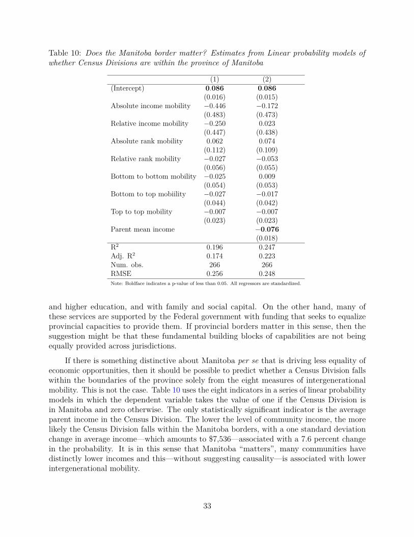
Table 10: Does the Manitoba border matter? Estimates from Linear probability models ofwhether Census Divisions are within the province of Manitoba

(1) (2)(Intercept) 0.086 0.086

(0.016) (0.015)Absolute income mobility −0.446 −0.172

(0.483) (0.473)Relative income mobility −0.250 0.023

(0.447) (0.438)Absolute rank mobility 0.062 0.074

(0.112) (0.109)Relative rank mobility −0.027 −0.053

(0.056) (0.055)Bottom to bottom mobility −0.025 0.009

(0.054) (0.053)Bottom to top mobiility −0.027 −0.017

(0.044) (0.042)Top to top mobility −0.007 −0.007

(0.023) (0.023)Parent mean income −0.076

(0.018)R2 0.196 0.247Adj. R2 0.174 0.223Num. obs. 266 266RMSE 0.256 0.248Note: Boldface indicates a p-value of less than 0.05. All regressors are standardized.

and higher education, and with family and social capital. On the other hand, many ofthese services are supported by the Federal government with funding that seeks to equalizeprovincial capacities to provide them. If provincial borders matter in this sense, then thesuggestion might be that these fundamental building blocks of capabilities are not beingequally provided across jurisdictions.

If there is something distinctive about Manitoba per se that is driving less equality ofeconomic opportunities, then it should be possible to predict whether a Census Division fallswithin the boundaries of the province solely from the eight measures of intergenerationalmobility. This is not the case. Table 10 uses the eight indicators in a series of linear probabilitymodels in which the dependent variable takes the value of one if the Census Division isin Manitoba and zero otherwise. The only statistically significant indicator is the averageparent income in the Census Division. The lower the level of community income, the morelikely the Census Division falls within the Manitoba borders, with a one standard deviationchange in average income—which amounts to $7,536—associated with a 7.6 percent changein the probability. It is in this sense that Manitoba “matters”, many communities havedistinctly lower incomes and this—without suggesting causality—is associated with lowerintergenerational mobility.

33

6.3 The divided landscape of intergenerational mobility

While this two-fold division of the Canadian landscape is useful as a communication device topoint to the first priorities for future research and public policy concern, it does not representthe most accurate clustering of the Census Divisions. The dendrogram in Figure 7 can bereasonably viewed as suggesting a four-fold clustering: the grouping of Census Divisionshighlighted in Figure 8, with the rest of the country divided into three additional groups.22

This preferred four-fold grouping is mapped in Figure 9. It offers a more general, and atthe same time, a more nuanced picture of the landscape of income mobility in the country,than what any single indicator would suggest. This map is not the same as that for theintergenerational cycle of low income, or of rags to riches mobility, depicted in Figures 5 and6.

In this grouping much of Québec, particularly outside of the major urban areas, isdistinguished from Ontario, and belongs to a lower mobility cluster. In Figure 9, these CensusDivisions are labelled as Cluster 3. Cluster 1 consists of the more populated areas of Ontario,including all of Southern Ontario. These areas are grouped with large parts of Alberta andthe southern part of Saskatchewan. This is a high mobility cluster. It also includes Vancouver,the municipalities to the north and south of the island of Montréal, as well as Québec Cityand its environs. It includes the major metropolitan areas of the country with the exceptionof the island of Montréal, and the cities in the Atlantic provinces. The northern parts ofthe country are not grouped into a single cluster. In particular, it is noteworthy that thecommunities along the eastern shore of James Bay and Hudson Bay are distinct from thosein Ontario and Manitoba, belonging to a higher mobility cluster, labelled as Cluster 2, thatalso collects other parts of rural Canada, particularly in the Atlantic.

6.4 Correlates of mobility among Census Divisions

Figure 10 shows a clear positive relationship between the Census Division poverty rate andthe bottom quintile to bottom quintile transition probability. Children raised by low incomeparents are more likely to be low income adults when they are raised in regions with higherpoverty rates. The transition probability is noticeably higher when the Census Divisionpoverty rate is above about 17 percent, noticeably lower when it is below about 13 percent,but varies considerably between this range.23

Bivariate descriptions of this sort are a first step in determining causal relationships.Indeed, the portrait of the degree and nature of intergenerational income mobility across

22A fifth cluster consisting of a single Census Division is also indicated by the dendrogram, but it is aregion in the very north of the country with a small population, and its selection by the algorithm as a clusteronto itself likely reflects measurement issues, rather than any substantive differences.

23The Lowess line depicted in the figure is based upon unweighted estimation across 260 Census Divisions.Six regions in Yukon, Nunavut and the Northwest Territories are excluded from the figure because the LowIncome Cut-off is not calculated by Statstics Canada in these areas. The figure also omits a small number ofCensus Divisions with very high bottom-to-bottom quintile transition probabilities for the sake of exposition,though they are included in the estimation used to obtain the line.

34

Census Division Clusters(determined by HierarchicalAgglomorative Clustering)

1234unclassified

Figure 9: The divided landscape of intergenerational income mobility: four clusters of CensusDivisions as determined by agglomoarative hierarchial clustering

35

0.20

0.25

0.30

0.35

0.40

0.45

0.50

Poverty rate in the parent's generation(Percent of population in the Census Division below the LICO)

Probability ofintergenerational low income

5 10 15 20 25 30 35 40

50,000

10,000

1,000

Number of Childrenin bottom quintile families

Figure 10: The relationship between the intergenerational cycle of low income and CensusDivision poverty rates

36

the country in the previous sections immediately raises questions about the factors thatcharacterize high and low mobility communities. The relationship between community povertyand intergenerational poverty is certainly a policy relevant pairing that comes quickly to mind.But there are others. International comparisons have received a good deal of attention in partbecause they have motivated discussion over other correlates and causes of the significantdifferences between countries. Within country comparisons should do the same.

Canada generally ranks relatively well when compared to other OECD countries, as inthe Great Gatsby Curve, which depicts a positive relationship between the intergenerationalincome elasticity and the Gini coefficient measuring cross-sectional income inequality amongparent incomes. A correlation of this sort should not be given a causal interpretation, but inthis case the relationship is predicted by theory (Krueger (2012), Corak (2013; 2016b), Solon(2004; 2015)), and has spurred detailed research on groupings of countries most pertinent forpublic policy, as in Landersø and Heckman (2016) who contrast Denmark and the UnitedStates, and Bradbury et al. (2015) who compare the United States to Australia, Canada,and the United Kingdom. This said, the Great Gatsby Curve privileges only one measureof intergenerational mobility, the intergenerational income elasticity, and has—with theexception of Chetty et al. (2014, 1612–14)—not been examined within countries.

Table 11 presents correlation coefficients summarizing the linear bivariate relationshipbetween each of the eight statistics measuring mobility, and 21 characteristics of the CensusDivisions. Some of these characteristics are derived from the analytical files used in theanalysis, others are derived from the individual level micro-data associated with the 1986Census, the so-called “Long Form” Census questionnaire distributed to roughly one-in-fiveCanadians.24 The results are grouped into four broad categories, roughly corresponding tofour important aspects to which theory might be interpreted as drawing attention: povertyand inequality; family and demography; social capital; and the structure of labour marketsand opportunities for employment (Corak (2013)).

The correlations with the poverty rate and those with the Gini coefficient are presentedin the first two rows of the table. The Census Division poverty rate is not strongly associatedwith absolute and relative income mobility, but is associated with lower intergenerationalrank mobility and rags to riches movement. It is also associated, as Figure 10 suggests, withhigher cycles of poverty. The Great Gatsby Curve is evident across the Canadian landscape,a higher Gini in parent incomes being associated with a higher intergenerational incomeelasticity. This finding, that inequality is associated with lower mobility, is robust acrossall the indicators, the one exception being rags to riches movement. Higher inequality, asmeasured by the Gini, is associated with lower absolute and relative rank mobility, and highercycles of poverty and privilege.

The remaining characteristics in the first panel of the table are intended to clarify this bymeasuring other dimensions of inequality. The share of parents with income that places themin the middle of the national income distribution—between the 25th and 75th percentiles—is

24The results reported in the table are based upon data weighted by the number of children in each CensusDivision according to the analytical sample used in the previous section. The unweighted results differ, andare often heavily influenced by a few low population outliers.

37

Table 11: Correlates of intergenerational income mobility: correlation coefficients based onCensus Divisons weighted by number of children

Income mobility Rank mobility Directional mobilityAbsolute Relative Average Absolute Relative Rags to Cycle of Cycle of

Census Division Characteristic income income income rank rank riches poverty privilege(αj) (βj) (Yj) (aj) (bj) (P1,5) (P1,1) (P5,5)

Poverty rate (below low income cut-off) -0.045 0.012 -0.351 -0.335 0.273 -0.393 0.217 -0.212Gini coefficient (parent incomes) -0.278 0.294 -0.081 -0.184 0.427 0.038 0.252 0.352Parents between 25th and 75th percentiles 0.231 -0.243 -0.119 0.025 -0.171 -0.178 -0.164 -0.128Parent incomes at 50th to 25th percentile -0.58 0.561 -0.322 -0.398 0.522 -0.166 0.531 -0.012Parent incomes at 75th to 50th percentile -0.309 0.28 -0.458 -0.386 0.416 -0.283 0.309 -0.108Parent incomes at 90th to 50th percentile -0.187 0.174 -0.245 -0.276 0.366 -0.157 0.2 0.093Parent incomes at 99th to 50th percentile 0.022 0.014 0.199 0.094 0.149 0.262 -0.038 0.527

Less than high school -0.134 0.072 -0.808 -0.327 0.082 -0.391 0.214 -0.543Lone parents -0.121 0.124 0.229 -0.158 0.271 -0.102 0.252 0.219Not born in Canada 0.123 -0.064 0.632 0.465 -0.229 0.599 -0.146 0.598English mother tongue -0.046 0.066 0.182 0.256 -0.184 0.387 0.046 0.208French mother tongue 0.067 -0.097 -0.265 -0.308 0.182 -0.472 -0.047 -0.311Parents not married -0.174 0.182 0.42 -0.054 0.222 0.134 0.332 0.378Population 0.055 -0.007 0.434 0.24 0.022 0.37 -0.044 0.567Population 25 years and older 0.051 -0.004 0.419 0.226 0.028 0.353 -0.036 0.554Parents filing in french 0.063 -0.09 -0.231 -0.297 0.179 -0.452 -0.05 -0.287

Moved to Census division 0.074 -0.059 0.3 0.228 -0.236 0.295 -0.155 0.101Moved to Census sub division 0.097 -0.065 0.474 0.336 -0.26 0.45 -0.182 0.289

Employment in manufacturing 0.217 -0.234 -0.073 0.004 -0.098 -0.092 -0.113 -0.055Employment in primary sector -0.153 0.142 -0.467 -0.041 -0.043 -0.051 0.011 -0.29Employment in top ten 3-digit SICs -0.229 0.194 -0.533 -0.268 0.149 -0.304 0.204 -0.412

Note: Column entries are weighted correlation coefficients. Census Division characteristics are derived from administrative tax data and the 1986 Canadian Census.

generally associated with greater mobility. The proportion of middle income parents in theCensus Division is not, however, associated with absolute rank mobility, and is negativelylinked with rags to riches movement. An important result in this panel is that more inequalityin the bottom part of the parent income distribution, as measured by the ratio of parentincome at the 50th percentile to parent income at the 25th percentile in each Census Division,is strongly associated with lower mobility. This sort of inequality correlates with lower incomeand rank mobility in both an absolute and relative sense, and with cycles of poverty, but notat all with intergenerational privilege. Several of these correlation coefficients are greater than0.5, among the highest in the table. Top end inequality shows similar correlations, whethermeasured as the 75 to 50 or the 90 to 50 ratio. But inequality at the very top, the ratio ofincomes between the 99th percentile and the 50th percentile, only correlates with rags to richesmobility and the cycle of privilege. Inequality is negatively associated with intergenerationalmobility, but it is inequality in the bottom and middle parts of the distribution that mostmatter, not inequality at the very top end.

The second panel groups together a number of demographic and population characteristics.The majority of these are calculated from Census data and refer to population shares in each

38

Census Division: the share of the population 25 and older not having a high school diploma,the share of lone parent households, the share not born in Canada, and the share with Englishand with French mother tongue.25 While low education and lone parenthood are associatedwith lower intergenerational mobility, the share of immigrants in the Census Division showsan opposite tendency. The larger the share of the population not born in the country, thegreater the degree of mobility, and particularly so with respect to directional mobility. Theshare of immigrants is strongly positively associated with rags to riches movement and cyclesof high income, the correlation almost reaching 0.6. At the same time it shows a weaknegative correlation with intergenerational cycles of low income.

The third panel offers the correlations with two indicators of geographic mobility, theshare of the population in the Census Division who reported living in a different CensusDivision in the 1981 Census, and the share who reported living in a different Census subdivision. Coleman (1988) suggests that geographic mobility may serve as an indicator of socialcapital, the implication being that changing place breaks networks and access to broadercommunity resources. The indicators I offer are imperfect as they are not individual-levelmeasures of geographic mobility—whether or not the individuals in the analytical file moved—but rather community level characteristics. In this sense, a high proportion of residentswho moved into or within the region may reflect the degree to which the region is a pole ofgrowth and economic opportunity, as likely as it is to reflect a broader sense of communityand engagement. The correlations seem to suggest the former is more likely, with a highershare of movers to or within the Census division being associated with greater rank mobility,greater rags to riches movement, and lower cycles of low income. These patterns echo thosefor the share of immigrants in the Census Division.

The fourth and final panel presents a number of indicators of the structure of labourmarkets, specifically of the nature and diversity of employment opportunities: the proportionof those 25 years and older employed in the manufacturing sector, in the primary sector, andthe proportion working in the top-ten three-digit industries. The manufacturing share tendsto be associated with greater mobility, while the primary share with lower mobility. Thegreater the concentration of employment in a few industries, the lower the degree of mobility.

All of these findings are descriptive and leave open important questions about the causalmechanisms. How to think about the role of place in the process determining mobility is anopen question. Parents living in less rich or more unequal Census Divisions may differ alongsome unobserved dimensions from parents in other regions even if both groups have the samerank in the national income distribution. In this sense, geography is informative about theparents, a view that contrasts with one ascribing a causal role to place. The clearest exampleof this challenge might be the interpretation given to the strong positive correlation betweenthe share of immigrants in the Census Division and the degree of intergenerational mobility.On the one hand, immigrants may be a positively selected group of parents along somedimensions or characteristics that are particularly beneficial for the mobility of their children;on the other hand, immigrants may have more of a tendency to settle in larger urban areas,

25The variables “Parents not married” and “Parents filing in french” refer to the information on the taxform of the parents of the children making up the analytical file, while “Population” and “Population 25years and older” are estimates of the Census Division total population derived from the Census.

39

with more diversified employment opportunities and other resources that encourage mobilityof all children regardless of family background. Oreopoulos (2008) reviews this literaturefrom a Canadian perspective, suggesting that the causal role of place is less important inCanada than in the United States, but this is a topic that should be revisited in light of myfindings and data. For example, Chetty and Hendren (2017a; 2017b) use a clear identificationstrategy based on sibling differences to examine the causal role of place, finding that it isimportant and offering county level estimates of the causal impact of neighbourhoods for theUnited States.

7 Conclusion

The Canadian geography of economic opportunity is a landscape of considerable mobility, butalso of considerable diversity. The members of the cohort I examine have on average attainedadult incomes that surpass their parents, almost without regard to the community in whichthey were raised. This reflects both absolute growth in their incomes, and how strongly theirincome relative to the average is tied to their parents’ relative income.

There is also considerable rank mobility. Upward rank mobility is strong for childrenwhose parent’s were in the bottom half of the income distribution, though generally not sohigh as to imply a move into the top half of their income distribution. Overall the typicalchild raised in the bottom half of the income distribution, by parents who ranked at the 25th

percentile, can expect to rise almost 20 percentiles, but this varies depending upon place,amounting to almost nothing in some Census Divisions and to as many as 30 percentiles inothers. Broadly speaking, upward mobility from the bottom does not seem to be constrainedby the possibility that children raised by top income parents are likely to also be top incomeadults, but rather by the chances that children raised by bottom income parents have lowerchances of moving out of low income.

A significant majority of children of low income parents live in parts of the countrywhere their chances of growing up to be low income adults are greater than one-in-four, andfor many the chances of this intergenerational cycle of poverty are as high as one-in-three.In contrast, there are only 9 of 266 Census Divisions where the chances of rags to richesmovement are 20 percent or greater, everywhere else they are lower, with about one-third oflow-income children living in communities where the chances of rising to the top are less than10 percent. A rather small fraction of the low income population, less than 3 percent, facevery limited opportunity to move up the economic ladder. But they are a telling group, livingin communities with relatively low average incomes. Even though large swaths of Manitobaform part of this landscape, provincial boundaries should not be considered as demarcatingadvantaged from less advantaged communities.

The Canadian landscape of economic opportunity is divided into four non-contiguousareas. Low mobility regions tend to be outside of urban areas, distant from poles of growth,while high mobility regions tend to be urban, or close to major urban ares, but not exclusivelyso with children growing up in many regions throughout Alberta and Saskatchewan beingamong the most mobile.

40

In uncovering these descriptive findings I make use of a large bank of administrative dataassociated with the Canadian income tax system that continues to offer potential to morethoroughly explore these issues. My analysis addresses a number of potential measurementproblems, but just as importantly recognizes that intergenerational mobility can be measuredin a host of different ways. While economic theory offers some guidance for empirical research,the subject of intergenerational mobility is both inherently multi-disciplinary and of ongoingpublic policy concern, implying that this guidance is less than complete.

For this reason I am agnostic with respect to an appropriate metric, which in turnsuggests the need for more research to assess the nature of the relationship between income,rank, and directional mobility. It is natural for policy makers to give priority to upwardmobility among the poor, but this has both an absolute and relative dimension. Friedman(2006, 95) recognizes that these dimensions may well be substitutes in the minds of manycitizens, suggesting that most

favor equal opportunity and fairness in the abstract sense that they would certainlysupport furthering these aims if doing so implied no risk, and no other cost, tothemselves. But in practice, taking more steps to move a society toward greaterfairness or more equal opportunity typically does impose risks, as well as costs, onat least some people. The importance of economic growth for this purpose is thatrising incomes make people more willing to accept these risks and costs in theinterest of what they take to be a better society for themselves as well as others.

Empirical research needs more guidance in appreciating the welfare implications of the hostof statistical indicators that are used in the literature. These implications very much remainan open issue in the interpretation of my descriptive results.

But this also suggests that attempts at interpreting the diversity in the findings needto appreciate the nature of economic growth, its variation across the country, and thepossible spatial auto-correlation it may imply. This is an aspect of my findings that meritscloser attention, and is clearly hinted at by the suggestion that the country contains fourbroad landscapes of economic opportunity. The suggestion that some parts of southwesternOntario cluster into a highly mobile landscape, in spite of declining fortunes associated withrestructuring of the manufacturing sector, may have something to do with the nature ofgrowth in Toronto and its proximity. The costs of moving to capture opportunity may berelatively lower than in more outlying areas, underscoring the importance of both growth andgeographic mobility. OECD (2016) recognizes that the nature of growth in cities is importantfor fostering inclusion and creating opportunity, and the experience of regions surroundingToronto may hint at the importance of this auto-correlation.

There are also important issues raised concerning the interpretation of the results insome rural and outlying communities. There is considerable diversity of mobility in manyareas of the country not near large metropolitan areas, suggesting that poles of growth andmobility are associated with more than proximity to large urban areas. Growing up in largesections of Alberta and Saskatchewan leads to among the highest rates of intergenerationalmobility in the country. My division of the Canadian landscape into a landscape of “us andthem” highlights areas that should be a first priority for future research. One response is to

41

suggest that this is associated with the experiences of some aboriginal communities, and thismay be particularly germane to my demarcation of large parts of Manitoba being part of anextremely low mobility cluster of Census Divisions. But at the same time many first nationscommunities are not part of this cluster, and the contrasts between them and others requiresmore detailed study.

Finally, I uncover some general patterns suggesting avenues for further research bydocumenting the bivariate correlations between mobility and a host of Census Division char-acteristics. There are strong correlations between intergenerational mobility and communitylevel income inequality, demographics, and labour market opportunities. Regions with highermobility tend to be regions with lower poverty and less income inequality. Higher incomeinequality in the lower half of the income distribution is strongly associated with lowermobility, almost regardless of which statistic is used to measure the child’s outcome. Higherincome inequality in the upper half of the income distribution is also associated with lowermobility, with the exception of top end inequality. I link information from the 1986 Censusto these tax data at the Census Division level to also show significant correlations betweenmobility and community demographic and labour market characteristics. Census Divisionswith a higher share of the population not born in the country tend to be higher mobilitycommunities, as do those with more diversified employment opportunities.

42

Appendix

The creation of the data and its representativeness

The algorithm used to construct the Intergenerational Income Data (IID) is described in theappendix to Corak and Heisz (1999), and further detail is given in Statistics Canada (undated).I first developed the IID with colleagues at Statistics Canada in the mid 1990s for the study ofintergenerational income dynamics. The data have since been updated in a number of ways, mostnotably by adding more annual observations on income as they have become available through thetax files submitted to Statistics Canada from the Canada Revenue Agency.

The algorithm creating the file links income tax information (the T1 form) for the members ofparticular age cohorts through time, and to their parents whose T1 forms are also tracked throughtime. The data used in this paper are made up of two cohorts of men and women whose T1 formswere linked, mostly through their Social Insurance Numbers, to their parents’ T1 forms: those 16 to19 years old in 1982, and those 16 to 19 years old in 1986. The matching process between parentsand children involves up to five years of tax information in order to find a child filing for the firsttime (and hence having a Social Insurance Number) while still at home according to their tax filingbehaviour. For example, the 1982 cohort refers to those individuals who were 16 to 19 years of age in1982 and who filed a T1 form while at home at some point between 1982 and 1986. In a similar way,the 1986 cohort refers to those in this same age bracket who first filed taxes at some point between1986 and 1990. It is necessary that individuals file an income tax return while still at home in orderto establish a link between their Social Insurance Numbers and the Social Insurance Numbers oftheir parents. This permits the longitudinal tracking of family members. Individuals who did notfile an income tax return while still at home are not included in the IID. Parental T1 forms areavailable from 1978, though the first possible year that children can be linked to their parents is1982. Both parents and children are followed through their T1 forms up to 2008, when the childrenare between the ages of 38 and 45. In addition, the T1 forms of the married and common-lawpartners of the children are also obtained from the disclosure of their Social Insurance Numbers onthe child’s adulthood T1 form. The spousal information, however, is available beginning only in1998. At the time this study began the 2009 income tax data were available only in a preliminaryversion, and therefore not used.

The coverage of the underlying target populations varies. Detailed examinations based upona comparison with the Census reveals an under-reporting of children with lower income parents,and those living in large metropolitan areas. The former likely reflects the tendency of childrenfrom lower income families to leave home at a younger age, and the later an under-representationof immigrants who arrived in the country in subsequent years and whose parents came to thecountry after the mid 1980s. The immigrant under-representation is the natural outcome of usinga longitudinal data set, and is not a concern as these cohorts of parents are likely not to haveany Canadian tax-based income when the children were growing up. Weights calculated from theCensus and additional sub-national information on reporting patterns across the income distributionhave been derived, and are used throughout the analysis. Past research estimating national levelstatistics has generally found that it makes little difference whether or not the weights are used.Oreopoulos (2003) pays particular attention to these issues of under-representation in the context ofa study focused on Toronto, and confirms the representativeness of the data. But more caution maywarranted when the objective is to cover the entire country at a relatively fine geography.

43

The creation of the weights

The derivation of the weights is described by Cook and Demnati (2000). The weights are constructedusing the 1986 Census and the Longitudinal Administrative Databank (LAD): the former offers ananchor for the population estimates, and the latter allows adjustments by family income. The LADis a 10 percent sample of the T1 Family File (T1FF) and includes all children who are dependentsof their tax-filing parents regardless of whether or not they (the children) filed taxes or not. In thissense it is more encompassing than the IID, which is also drawn from the T1FF. However, somechildren are imputed in the LAD based upon other tax and benefit information. This is one reasonwhy it is not an appropriate source for intergenerational mobility studies, along with the fact that itis a one-in-ten sample of T1 filers, and offers limited information on the child’s gender.

The weights are derived by using only children from the LAD between the ages of 16 and 19 foreach cohort, including tax filing and non-filing dependent children. This data allows a comparison ofIID under-coverage according to parental income. Eleven income classes based on the parental totalmarket income, in bands of $10,000 and including $100,000 and over, are defined for geographicareas determined by the first two digits of the postal code. Some aggregation of adjacent areas wasundertaken when the number of observations proved to be very small. This involved the aggregationof 36 areas into 12, and combining the Yukon, Northwest Territories, and Nunavut into one area.This is to say that while the weights are distinguished by parental income, this is done withingeographic areas broader than the Census Division.

Weighted counts are derived from the LAD for each cohort, by income class and these geographicareas. The counts are then used in conjunction with the 1986 Census to adjust for gender, a variablenot available in the LAD because some children are imputed. The IID was adjusted with 1986Census data by age, and for under or over-coverage of the Canadian population by the tax system.This leads to estimates of the number of children by province, age in 1986, and gender, using aweighted 20 percent file from the 1986 Census. Another set of counts are made from the IID usingthe basic weight created in the step outlined in the previous paragraph. These counts were made byage in 1986, gender, and province. A census adjustment factor is computed using these counts. Thefinal weight is constructed by multiplying the basic weight, from the first step, with the adjustmentfactor, from the second step. Cook and Demnati (2000) describe the method. The point is that theweighted counts from the IID are meant to be representative of the Canadian population belongingto these cohorts, accounting for gender, geography, and parental income.

Assigning Census geographic information

The postal code is a six character identifier developed and used by Canada Post Corporation formail sorting and delivery, and takes the form AnA nAn where A represents an alphabetic characterand n is a numeric character between 0 and 9. The first three characters are referred to as theForward Sortation Area (FSA), and the latter three as the Local Delivery Unit (LDU). The postalcode became universal on the T1 files beginning in 1982. Every record in the Family File, thecomponent of the IID containing the explicit link between a child and his or her parents, was linkedto the underlying T1 records for the year the child was first matched to his or her parents. If thefamily members were first matched by the algorithm in 1982 then the postal code for that year isused as the basis for linking Census information to the IID.

Statistics Canada (undated) describes the process used in converting this information to Census

44

geography codes. The following summary is extracted from this source. All family members shouldhave the same postal code on the assumption that they are co-resident. In fact this is the casefor 3,227,271 of the 3,463,712 family records in the full file. Of the 236,441 families reporting atleast one different postal code between the members, 190,608 had at least 2 identical postal codesand this is was used as the family postal code. The remaining 45,833 families are put aside as a“problem” file requiring special consideration. An examination of these records showed that 26,876had at least two identical Forward Sortation Areas, and this is used as the basis for constructingthe family postal code if the LDU was the same across the family members. A similar process wasbased on the LDU: 6,008 records had at least two family members reporting the same LDU, andthis is used as the last three digits if the FSA was reported to be the same across family members.This left 12,949 records. If the postal code was not missing for these records, then the postal codeof the father was used. If it was missing, that of the mother was used, and finally if that was alsomissing the postal code reported by the child is used. If all of these codes are missing the family’spostal code was assigned to be missing, with 1,063 records falling into this last category.

Postal Codes do not necessarily correspond with the boundaries of the geographic units used bythe Census. The Postal Code Conversion File (the GEORES3C Program), a SAS program writtenby Russell Wilkins of Statistics Canada to perform automated Census geographic coding from a listof postal codes, is used to append Census geography codes. The complete set of records processedby this program had 3,463,712 records, and of these 30,300 proved to be problematic and requiredfurther processing. In the end only 11 of these could not be assigned a valid geographic code.The Postal Code Conversion File added 1996 Census information to the Family File, and this wasconverted to 1986 Census information using an auxiliary program (EA96286) also written by RussellWilkins. Version 3 of this program, written in 1998, was used. For more detail, see the StatisticsCanada website: Postal Code Conversion File (PCCF), Reference Guide, 2013. Statistics CanadaCatalogue no. 92-154-G, accessed at http://www.statcan.gc.ca/pub/92-154-g/92-154-g2013001-eng.pdf [accessed on May 14, 2015].

Census geographic coding

The Census of Canada is organized along three different geographic hierarchies: a national hierarchycovering the entire country; a metropolitan hierarchy that applies to urban areas; and a postalcode hierarchy based on the Canada Post Corporation coding. The Enumeration Area is the basicbuilding block that is nested within other broader geographic areas of the national hierarchy. Thereare 44,042 Enumeration Areas in the 1986 Census. The Census subdivision (CSD) refers to what inmany provinces are legislated to be municipalities, or equivalent legislated areas like reserves orsettlements. In Newfoundland and Labrador, Nova Scotia and British Columbia a CSD refers to ageographic area created by Statistics Canada in cooperation with these provinces as equivalent tomunicipalities for statistical purposes. The Census Division (CD) is the next broadest geographicunit in the national hierarchy, and refers to legislatively determined areas such as counties, regionaldistricts, regional municipalities or other legislated areas at the provincial level. For the mostpart their boundaries are established by provincial law for regional planning and the provision ofservices. These areas are not legislated in four provinces—Newfoundland and Labrador, Manitoba,Saskatchewan, and Alberta—and have been created by Statistics Canada for the purposes of datadissemination. There were 266 CDs in the 1986 Census. The CSD is nested within the CD, whichin turn is nested within the broadest unit within the province, the Economic Region. The EconomicRegion is not defined for the 1986 Census, first appearing as a geographic category in the 1996

45

Census. The Census geography hierarchies as they existed in 1986 are described in Statistics Canada(1987).

The analysis in this paper uses the national hierarchy at the provincial and Census Divisionlevel. Information at the Census subdivision level is also derived, but used and presented in futureresearch only for Census Divisions with larger populations. This information is available as aspreadsheet at MilesCorak.com/Equality-of-Opportunity.

Data quality issues

I create a number of different analytical files that allow me to assess the robustness of the analysis.The first alternative file includes all incomes, rather than using a lower cut-off of $500 as the basisof selection into the analytical file. The second alternative is based upon this cut-off but includesonly the 1986 cohort of individuals. I point out below that their geographic locations as teenagersmight be considered to be more accurately determined. In similar ways, alternative files are alsodeveloped for boys and girls separately. The core of the analysis, that reported in the text, is basedupon the file that uses all cohorts. This maximizes the sample size, and maintains an income cut-offof $500 because this is a better approximation of permanent income, avoiding measurement error inthe lower end of the distribution and permitting the derivation of logarithms used in the assessmentof income mobility. I also create similar analytical files from the 1986 cohort that is based on thechildren being 31 and 32 years of age. These alternatives allow me to assess measurement issuesassociated with life-cycle biases, and make comparisons to a similarly aged cohort used by Chettyet al. (2014).

As alluded to, the IID weights will not perfectly correspond with the sub-national geographyat which the analysis is actually conducted. The weights are based upon province and broad regionsdefined by the first two digits of the postal code. As a result, there is no guarantee that weightedpopulation counts from the IID will correspond with Census counts for areas as small as the Censussubdivision. For this reason the analysis has been conducted at a level no finer than the CensusDivision, and with both weighted and unweighted data. This paper reports only the results fromthe weighted data, the choice not making substantive differences.

Figure 11, however, illustrates an important data concern by presenting a very loosely definedestimate of the “coverage ratio” for each Census Division, based upon the analytical file used in theanalysis. This is the ratio of the population estimate in the tax-based analytical files—unweightedand weighted—to the population estimate for this age cohort of Canadians as derived from the 1986Census. These should be loosely interpreted. For example, it is not clear that these ratios shouldbe equal to one since the analytical file is based on a number of selection rules to ensure that theindividuals are still alive and present in Canada in the five year period ending in 2008, and alsothat a reasonable estimate is made of their permanent incomes. The unweighted coverage ratiosrange from as low as 0.3 to as high as 0.85, and on average are 0.64. The weighted ratios are, as theFigure also shows, higher, and on average are equal to 1. But many are greater than one, thoughmost range between 0.75 and 1.25. This requires an explanation.

There are two reasons these ratios deviate from one. To some degree it reflects the slippagebetween the way in which the weights are calculated according to the first two digits of the postalcode, while the placement of children into particular Census Divisions is done according to thefull six-digit postal code. There are 9 Census Divisions in which the ratio of population weighted

46

0 50 100 150 200 250

0.5

1.0

1.5

266 Census Divisions ordered fromlowest to highest coverage ratio (unweighted data)

Rat

io o

f sam

ple

popu

latio

n in

tax

data

to C

ensu

s es

timat

e

Weighted dataUnweighted data

Figure 11: Coverage ratios of the population of children in each of 266 Census Divisions:ratio of sample population in tax data relative to Census estimate, weighted and unweighted

47

Table 12: Census Divisions in which the ratio of weighted sample population in tax data to1986 Census estimate of children born between 1963 and 1970 is less than 0.75

Administrative Data 1986 Census Ratio weightedCensus Division, Province/Territory Weighted Unweighted Total to Census

Division No. 23 MB 725 525 1,575 0.47Division No. 15 AB 1,950 1,275 3,925 0.50Division No. 14 AB 1,850 1,100 3,325 0.56Territoire-du-Nouveau-Quebec QC 3,150 1,950 5,625 0.56Sunbury County NB 2,300 1,875 3,800 0.60Division No. 18 SK 2,575 1,325 4,175 0.62Division No. 22 MB 3,250 2,075 5,150 0.63Central Coast Regional District BC 300 125 400 0.72Kitikmeot Region NT 525 225 700 0.75

Note: All numbers are rounded to the nearest 25.

counts from the tax data to the Census data are less than 0.75, and 11 with ratios greater than 1.25.These groups of Census Divisions are listed, respectively, in Tables 12 and 13. The results for thesecommunities should be interpreted with caution, though they selectively continue to be includedin some of the results reported in this paper. In particular, they continue, with one exception, tobe included in the cluster analysis, where there is no explicit reporting or use of any one mobilitystatistic. All of these communities are very small in population for the age group of individuals thatis the focus of attention.

The second reason for the coverage ratios being very low or very high is related to howaccurately children may be placed in particular Census Divisions. This has to do with the child’s agein the year linked to the parents. Recall that children are assigned to a geographic area accordingto the postal code on the T1 files in the year they are linked by the IID algorithm to their parents.As suggested, at one extreme this involves using individuals who are 16 to 19 years of age in 1986,and linked to their parents in that year. Situating these children geographically with 1986 Censusinformation is probably an accurate link to the communities in which they were growing up betweenthe ages of 15 to 19, when parental income is measured. But at the other extreme the linkagealgorithm involves a cohort who were 16 to 19 years of age in 1982, and some being as old as 23when linked with their parents in 1986 and when the Census geography is also established. Somefraction of these children and their parents may well have been living in a different Census Divisionwhen the children were between 15 and 19, which would date from 1982 and earlier. This raises aquestion as to how accurately the region in which they actually lived is captured by ascribing themto a Census Division in 1986. Figure 12 illustrates by replicating Figure 11 for the youngest cohortin the IID, those who were 16 to 19 in 1986. The weighted coverage ratios are much more likely tobe less than one. There are 31 of 266 Census Divisions with a coverage ratio greater than one, andonly 2 with a ratio greater than 1.25.

However, the differences between the two samples described in Figures 11 and 12 don’t lead tosubstantive differences in the findings. When the results for all cohorts presented in the body of the

48

0 50 100 150 200 250

0.5

1.0

1.5

266 Census Divisions ordered fromlowest to highest coverage ratio (unweighted data)

Rat

io o

f sam

ple

popu

latio

n in

tax

data

to C

ensu

s es

timat

e

Weighted dataUnweighted data

Figure 12: Coverage ratios of the population of children 16 to 19 years of age in 1986 in eachof 266 Census Divisions: ratio of sample population in tax data relative to Census estimate,weighted and unweighted

49

0 50 100 150 200 250

0

10

20

30

40

50

60

266 Census Divisions ordered from highest to lowest relative mobility

Top

− b

otto

m d

iffer

ence

in p

erce

ntile

ran

ks

Canada, 24.2

Vertical lines indicate95% confidence interval

Estimate for 1986 cohortonly if statistically different

Figure 13: Least squares estimates of relative rank mobility for all children and for the subsetof those 16 to 19 years of age in 1986 in each of 266 Census Divisions

50

Table 13: Census Divisions in which the ratio of weighted sample population in tax data to1986 Census estimate of children born between 1963 and 1970 is greater than 1.25

Administrative Data 1986 Census Ratio weightedCensus Division, Province/Territory Weighted Unweighted Total to Census

Division No. 16 MB 1,450 950 1,150 1.25Richmond County NS 2,000 1,200 1,550 1.29Lotbiniere QC 5,350 2,650 4,100 1.30Division No. 18 MB 3,275 2,000 2,475 1.31Muskoka District Municipality ON 5,700 2,925 4,300 1.33Parry Sound District ON 5,150 2,775 3,825 1.35Portneuf QC 9,600 4,925 6,750 1.42Manitoulin District ON 1,725 725 1,200 1.44Montmorency No. 2 QC 1,100 550 725 1.51Napierville QC 2,825 1,575 1,825 1.53Montmorency No. 1 QC 4,375 2,150 2,750 1.60

Note: All numbers are rounded to the nearest 25.

paper are compared to those from the subset belonging to the 1986 cohort, there are differences, butgenerally only to the extent that might be expected from chance. Figure 13 offers one illustration.The data in this Figure contrast least squares estimates of relative rank mobility—100× bj—betweenthe two samples used in Figures 11 and 12. The vertical lines represent the 95 percent confidenceinterval around the estimated bj for the full sample. The estimates for the 1986 cohort and theirconfidence intervals are presented only for those Census Divisions in which the null hypothesisof no difference between the estimates can be rejected. Relative rank mobility is estimated to bestatistically different—as determined by a z-test at the 95 percent confidence level—between thesetwo samples in 14 of the 266 Census Divisions. This is not greater than what would be expected bychance. This said, when the estimates are found to be statistically different, they tend to be higherusing the 1986 cohort in all but 2 cases.

An online appendix available at MilesCorak.com/Equality-of-Opportunity replicates all thetables and figures in the text using the younger cohort. The differences do not overturn the majorconclusions. This said, there are some differences in the classification of Census Divisions into theparticular groupings used to create the maps and some tables. These groupings are not based onany notion of statistical significance, so slight differences in the values of the statistics around thecut-offs defining the groupings, may lead to different classifications. The most important substantivedifference is the clustering of the 266 Census Divisions into four groupings, as mapped in Figure9. The online appendix also separately compares each of the eight mobility statistics used in theclustering. In general, there is no systematic difference between the two sets of statistics with theexception of the estimates for absolute income mobility and for the average parent income in theCensus Division. Both these statistics show a tendency to be higher when the full sample is used.This may also influence the classifications resulting from the clustering algorithm. However, in somesense this result is to be expected given that the children and their parents have a tendency to beolder in the full sample, and as a result likely to be earning slightly higher incomes.

51

References

Atkinson, Anthony B., A.K. Maynard, and C.G. Trinder. 1983. Parents and Children:Incomes in Two Generations. London: Heinemann Educational Books.

Becker, Gary S., and Nigel Tomes. 1979. “An Equilibrium Theory of the Distribution ofIncome and Intergenerational Mobility.” Journal of Political Economy 87 (6): 1153–89.http://www.jstor.org/stable/1833328.

———. 1986. “Human Capital and the Rise and Fall of Families.” Journal of LaborEconomics 4 (3, Part 2): S1–S39. doi:10.1086/298118.

Becker, Gary, Scott Duke Kominers, Kevin M. Murphy, and Jörg L. Spenkuch. 2015. “ATheory of Intergenerational Mobility.” Munich, Germany: MPRA Research Paper No.66334. https://mpra.ub.uni-muenchen.de/66334/.

Beland, François. 1987. “A Comparison of the Mobility Structure of Francophones andAnglophones in Quebec: 1954, 1964, 1974.” Canadian Review of Sociology and Anthropology24 (2): 232–51.

Bhattacharya, Debopam, and Bhashkar Mazumder. 2011. “A Nonparametric Analysisof Black–white Differences in Intergenerational Income Mobility in the United States.”Quantitative Economics 2 (3): 335–79. doi:10.3982/QE69.

Björklund, Anders, and Markus Jäntti. 2011. “Intergenerational Income Mobility and theRole of Family Background.” In The Oxford Handbook of Economic Inequality, edited byWiemer Salverda, Brian Nolan, and Tim Smeeding. Oxford: Oxford University Press.

Black, Sandra E., and Paul J. Devereux. 2011. “Recent Developments in IntergenerationalMobility.” In Handbook of Labor Economics, edited by David Card and Orley Ashenfel-ter, 4, Part B:1487–1541. Elsevier. http://www.sciencedirect.com/science/article/pii/S0169721811024142.

Blanden, Jo. 2005. “Love and Money: Intergenerational Mobility and Marital Matching onParental Income.” Research Paper No. 272. Ottawa: Statistics Canada.

———. 2013. “Cross-Country Differences in Intergenerational Earnings Mobility: A Com-parison of Approaches from Economics and Sociology.” Journal of Economic Surveys 27(1): 38–73. doi:10.1111/j.1467-6419.2011.00690.x.

Blau, Peter Michael, and Otis Dudley Duncan. 1978. The American Occupational Structure.New York: Free Press.

Boyd, Monica, John Goyder, Frank E. Jones, Hugh A. McRoberts, Peter C. Pineo, and JohnPorter. 1981. “Status Attainment in Canada: Findings of the Canadian Mobility Study.”Canadian Review of Sociology and Anthropology 18 (5): 657–73.

Bradbury, Bruce, Miles Corak, Jane Waldfogel, and Elizabeth Washbrook. 2015. Too ManyChildren Left Behind: The U.S. Achievement Gap in Comparative Perspective. New York:

52

Russell Sage Foundation.

Brown, Ashton. 2011. “Intergenerational Mobility in Canada: Earnings Persistence andthe Role of Education.” Princeton N.J.: Princeton University, Department of Economics;Undergraduate thesis.

Carney, Mark. 2014. “Inclusive Capitalism: Creating a Sense of the Systemic.” London:Bank of England, Speech given by Mark Carney, Governor of the Bank of England atthe Conference on Inclusive Capitalism. http://www.bankofengland.co.uk/publications/Documents/speeches/2014/speech731.pdf.

Caucutt, Elizabeth, and Lance Lochner. 2017. “Early and Late Human Capital Invetments,Borrowing Constraints, and the Family.” Working Paper 2017-040. Chicago: HumanCapital & Economic Opportunity Global Working Group.

Chen, Wen-Hao, Yuri Ostrovsky, and Patrizio Piraino. 2017. “Lifecycle Variation, Errors-in-Variables Bias and Nonlinearities in Intergenerational Income Transmission: New Evidencefrom Canada.” Labour Economics 44 (1): 1–12.

Chetty, Raj, and Nathaniel Hendren. 2017a. “The Impacts of Neighborhoods on Intergenera-tional Mobility I: Childhood Exposure Effects.”

———. 2017b. “The Impacts of Neighborhoods on Intergenerational Mobility II: County-Level Estimates.”

Chetty, Raj, David Grusky, Maximilian Hell, Nathaniel Hendren, Robert Manduca, andJimmy Narang. 2017. “The Fading American Dream: Trends in Absolute Income MobilitySince 1940.” Science 356 (6336): 398–406. doi:10.1126/science.aal4617.

Chetty, Raj, Nathaniel Hendren, and Lawrence F. Katz. 2016. “The Effects of Exposureto Better Neighborhoods on Children: New Evidence from the Moving to OpportunityExperiment.” American Economic Review 106 (4): 855–902. doi:10.1257/aer.20150572.

Chetty, Raj, Nathaniel Hendren, Patrick Kline, and Emmanuel Saez. 2014. “Where Is theLand of Opportunity? The Geography of Intergenerational Mobility in the United States.”Quarterly Journal of Economics 129 (4): 1553–1623. doi:10.1093/qje/qju022.

Coleman, James S. 1988. “Social Capital in the Creation of Human Capital.” AmericanJournal of Sociology 94 (Supplement): S95–S120.

Cook, K., and A. Demnati. 2000. “Weighting the Intergenerational Income Data File.”Unpublished, 10 pages. Statistics Canada, Social Surveys Methods Division.

Corak, Miles. 2001a. “Are the Kids All Right: Intergenerational Mobility and Child Well-Being in Canada.” In Review of Economic Performance and Social Progress, edited byKeith Banting, Andrew Sharpe, and France St-Hilaire. Montreal; Ottawa: Institute forResearch on Public Policy; Centre for the Study of Living Standards.

———. 2001b. “Death and Divorce: The Long-Term Consequences of Parental Loss onAdolescents.” Journal of Labor Economics 19 (3): 682–715. http://www.jstor.org/stable/

53

10.1086/322078.

———. 2006. “Do Poor Children Become Poor Adults? Lessons from a Cross CountryComparison of Generational Earnings Mobility.” In Research on Economic Inequality,edited by In John Creedy and Guyonne Kalb. Vol. 13. Amsterdam: Elsevier.

———. 2013. “Income Inequality, Equality of Opportunity, and Intergenerational Mobility.”Journal of Economic Perspectives 27 (3): 79–102. doi:10.1257/jep.27.3.79.

———. 2016a. “How Much Social Mobility: More, but Not Without Other Things.” In TheUs Labor Market: Questions and Challenges for Public Policy, edited by Michael R. Strain.Washington: American Enterprise Institute.

———. 2016b. “How the Great Gatsby Curve Got Its Name.” https://milescorak.com/2016/12/04/how-the-great-gatsby-curve-got-its-name/.

———. 2016c. “Economic Theory and Practical Lessons for Measuring Equality of Opportu-nities.” OECD Statistics Working Papers No. 2016/02. Paris: Organization for EconomicCooperation & Development.

Corak, Miles, and Andrew Heisz. 1998. “How to Get Ahead in Life: Some Correlates ofIntergenerational Income Mobility in Canada.” In Labour Markets, Social Institutions, andthe Future of Canada’s Children, edited by Miles Corak. Catalogue No. 89-553. Ottawa:Statistics Canada.

———. 1999. “The Intergenerational Earnings and Income Mobility of Canadian Men:Evidence from Longitudinal Income Tax Data.” The Journal of Human Resources 34 (3):504–33. http://www.jstor.org/stable/146378.

Corak, Miles, and Patrizio Piraino. 2011. “The Intergenerational Transmission of Employers.”Journal of Labor Economics 29 (1): 37–68. http://www.jstor.org/stable/10.1086/656371.

———. 2016. “The Inheritance of Employers and Nonlinearities in Intergenerational EarningsMobility.” In Inequality and Growth: Patterns and Policy, edited by Kaushik Basu andJoseph Stiglitz. London: Palgrave Macmillan.

Corak, Miles, Bjorn Gustafsson, and Torun Osterberg. 2004. “Intergenerational Influences onthe Receipt of Unemployment Insurance in Canada and Sweden.” In Generational IncomeMobility in North America and Europe, edited by Miles Corak. Cambridge: CambridgeUniversity Press.

Corak, Miles, Matthew J. Lindquist, and Bhashkar Mazumder. 2014. “A Comparison ofUpward and Downward Intergenerational Mobility in Canada, Sweden and the UnitedStates.” Labour Economics 30: 185–200. doi:10.1016/j.labeco.2014.03.013.

Creese, Gillian, Neil Guppy, and Martin Meissner. 1991. “Ups and Downs on the Ladder ofSuccess: Social Mobility in Canada.” Catalogue No. 11-612E, No. 5. Ottawa: StatisticsCanada.

Djabir, Kambi, and Maxime Fougère. 2017. “Intergenerational Mobility in Canada: NewEvidence on Educational Mobility.” Unpublished paper presented to the Meetings of

54

the Canadian Economics Association. Antigonish, Nova Scotia: Employment & SocialDevelopment Canada.

Durlauf, Steven N. 1996. “A Theory of Persistent Income Inequality.” Journal of EconomicGrowth 1 (1). Springer: 75–93. http://www.jstor.org/stable/40215882.

———. 2006. “Groups, Social Influences, and Inequality.” In Poverty Traps, edited bySamuel Bowles, Steven N. Durlauf, and Karla Hoff, 141–75. New York; Princeton N.J.:Russell Sage Foundation; Princeton University Press.

Economic Mobility Project, Pew Charitable Trusts. 2012. “Pursuing the AmericanDream: Economic Mobility Across Generations.” Washington: Pew CharitableTrusts. http://www.pewtrusts.org/en/research-and-analysis/reports/0001/01/01/pursuing-the-american-dream.

Erikson, Robert, and John H. Goldthrope. 1993. The Constant Flux: A Study of ClassMobility in Industrial Societies. Oxford: Clarendon Press.

Fortin, Nicole, and Sophie Lefebvre. 1998. “Intergenerational Income Mobility in Canada.”In Labour Markets, Social Institutions, and the Future of Canada’s Children, edited byMiles Corak. Catalogue No. 89-553. Ottawa: Statistics Canada.

Friedman, Benjamin M. 2006. The Moral Consequences of Economic Growth. New York:Alfred A. Knopf.

Furman, Jason. 2016. “Equality and Efficiency: A Global Perspctive.” https://obamawhitehouse.archives.gov/sites/default/files/page/files/20160502_wb_mfm_forum_cea.pdf.

Grawe, Nathan D. 2004. “Reconsidering the Use of Nonlinearities in IntergenerationalEarnings Mobility as a Test for Credit Constraints.” The Journal of Human Resources 39(3): 813–27. http://www.jstor.org/stable/3558998.

———. 2006. “Lifecycle Bias in Estimates of Intergenerational Earnings Persistence.” LabourEconomics 13 (5): 551–70. doi:10.1016/j.labeco.2005.04.002.

Güell, Maia, Michele Pellizzari, Giovanni Pica, and José V. Rodríguez Mora. 2015. “Corre-lating Social Mobility and Economic Outcomes.” Unpublished. University of Edinburgh.

Haider, Steven, and Gary Solon. 2006. “Life-Cycle Variation in the Association BetweenCurrent and Lifetime Earnings.” The American Economic Review 96 (4): 1308–20.http://www.jstor.org/stable/30034342.

Han, Song, and Casey B. Mulligan. 2001. “Human Capital, Heterogeneity and EstimatedDegrees of Intergenerational Mobility.” The Economic Journal 111 (470): 207–43. http://www.jstor.org/stable/2667863.

Hanushek, Eric A., Charles Ka Yui Leung, and Kuzey Yilmaz. 2014. “Borrowing Constraints,College Aid, and Intergenerational Mobility.” Journal of Human Capital 8 (1): 1–41.doi:10.1086/675501.

Hastie, Trevor, Robert Tibshirani, and Jerome Friedman. 2009. The Elements of Statistical

55

Learning: Data Mining, Inference, and Prediction. Second Edition. New York: Springer.

Heckman, James J. 2008. “Schools, Skills, and Synapses.” Economic Inquiry 46 (3). BlackwellPublishing Inc: 289–324. doi:10.1111/j.1465-7295.2008.00163.x.

Heckman, James J., and Stefano Mosso. 2014. “The Economics of Human Development andSocial Mobility.” Cambridge, Mass.: NBER Working Paper Series No. 19925.

Heidrich, Stefanie. 2015. “Intergenerational Mobility in Sweden: A Regional Perspec-tive.” Unpublished mimeo. https://www.researchgate.net/publication/283119232_Intergenerational_Mobility_in_Sweden_a_Regional_Perspective.

Isajiw, Wsevolod W., Aysan Sev’er, and Leo Driedger. 1993. “Ethnic Identity and SocialMobility: A Test of the ‘Drawback Model’.” Canadian Journal of Sociology. 18 (2): 177–96.

Jäntti, Markus, Bernt Bratsberg, Knut Røed, Oddbjørn Raaum, Robin Naylor, Eva Öster-backa, Anders Björklund, and Tor Eriksson. 2006. “American Exceptionalism in a NewLight: A Comparison of Intergenerational Earnings Mobility in the Nordic Countries, theUnited Kingdom and the United States.” IZA Disscussion Paper No. 1938. Institute for theStudy of Labor. http://www.iza.org/en/webcontent/publications/papers/viewAbstract?dp_id=1938.

Jencks, Christopher, and Laura Tach. 2006. “Would Equal Opportunity Mean More Mobility?”In Mobility and Inequality, edited by David B. Gursky Morgan Stephen L. and Gary S.Fields. Stanford: Stanford University Press.

Jenkins, Stephen. 1987. “Snapshots Versus Movies.” European Economic Review 31 (5):1149–58. doi:10.1016/S0014-2921(87)80010-7.

Krueger, Alan B. 2012. “The Rise and Consequences of Inequality in the United States.”https://obamawhitehouse.archives.gov/sites/default/files/krueger_cap_speech_final_remarks.pdf.

Landersø, Rasmus, and James J. Heckman. 2016. “The Scandinavian Fantasy: The Sources ofIntergenerational Mobility in Denmark and the U.S.” Scandinavian Journal of Economics118 (4): 794–846. doi:10.1111/sjoe.12219.

Lindahl, Mikael, Mårten Palme, Sofia Sandgren-Massih, and Anna Sjögren. 2014. “A Testof the Becker-Tomes Model of Human Capital Transmission Using Microdata on FourGenerations.” Journal of Human Capital 8 (1): 80–96. doi:10.1086/674104.

———. 2015. “Long-Term Intergenerational Persistence of Human Capital: An Em-pirical Analysis of Four Generations.” Journal of Human Resources 50 (1): 1–33.doi:10.3368/jhr.50.1.1.

Loury, Glenn C. 1981. “Intergenerational Transfers and the Distribution of Earnings.”Econometrica 49 (4): 843–67. http://www.jstor.org/stable/1912506.

McRoberts, Hugh, and Kevin Selbee. 1981. “Trends in Occupational Mobility in Canadaand the United States: A Comparison.” American Sociological Review. 46: 406–21.

Milanovic, Branko. 2016. “The Downside of Upward Mobility.” http://glineq.blogspot.ca/

56

2016/09/the-downside-of-upward-mobility.html.

Mulligan, Casey B. 1997. Parental Priorities and Economic Inequality. Chicago: Universityof Chicago Press.

Nybom, Martin, and Jan Stuhler. 2015. “Biases in Standard Measures of IntergenerationalIncome Dependence.” Working Paper Number 2015:13. Institute for Evaluation of LaborMarket; Education Policy.

OECD. 2016. Making Cities Work for All: Data and Actions for Inclusive Growth. Paris:OECD Publishing. doi:10.1787/9789264263260-en.

Oreopoulos, Philip. 2003. “The Long-Run Consequences of Living in a Poor Neighborhood.”The Quarterly Journal of Economics 118 (4): 1533–75. http://www.jstor.org/stable/25053946.

———. 2008. “Neighbourhood Effects in Canada: A Critique.” Canadian Public Policy 34(2): 237–58. doi:10.3138/cpp.34.2.237.

Oreopoulos, Philip, Marianne Page, and Ann Huff Stevens. 2008. “The IntergenerationalEffects of Worker Displacement.” Journal of Labor Economics 26 (3): 455–83. http://www.jstor.org/stable/10.1086/588493.

Ostrovsky, Yuri. 2017. “Doing as Well as One’s Parents? Tracking Recent Changes inAbsolute Income Mobility in Canada.” Economic Insights, no. 11-626-X (May). Ottawa:Statistics Canada. http://www.statcan.gc.ca/pub/11-626-x/11-626-x2017073-eng.htm.

O’Neill, Donal, Olive Sweetman, and Dirk Van de gaer. 2007. “The Effects of MeasurementError and Omitted Variables When Using Transition Matrices to Measure IntergenerationalMobility.” The Journal of Economic Inequality 5 (2): 159–78. doi:10.1007/s10888-006-9035-7.

Reeves, Richard V. 2016. Dream Hoarders: How the American Upper Middle Class Is LeavingEveryone Else in the Dust, Why That Is a Problem, and What to Do About It. WashingtonDC: Brookings Institution Press.

Roemer, John. 2004. “Equal Opportunity and Intergenerational Mobility: Going BeyondIntergenerational Income Transition Matrices.” In Generational Income Mobility in NorthAmerica and Europe, edited by Miles Corak. Cambridge: Cambridge University Press.

Saez, Emmanuel, and Stefanie Stantcheva. 2016. “Generalized Social Marginal Wel-fare Weights for Optimal Tax Theory.” American Economic Review 106 (1): 24–45.doi:10.1257/aer.20141362.

Solon, Gary. 1992. “Intergenerational Income Mobility in the United States.” The AmericanEconomic Review 82 (3): 393–408. http://www.jstor.org/stable/2117312.

———. 1999. “Intergenerational Mobility in the Labor Market.” In Handbook of LaborEconomics, edited by Orley C. Ashenfelter and David Card. Vol. 3A. Amsterdam: ElsevierScience.

———. 2002. “Cross-Country Differences in Intergenerational Earnings Mobility.” The

57

Journal of Economic Perspectives 16 (3): 59–66. http://www.jstor.org/stable/3216950.

———. 2004. “A Model of Intergenerational Mobility Variation over Time and Place.”In Generational Income Mobility in North America and Europe, edited by Miles Corak.Cambridge: Cambridge University Press.

———. 2015. “What Do We Know so Far About Multigenerational Mobility?” Cambridge,Mass.: NBER Working Paper Series No. 21053.

Statistics Canada. 1987. “1986 Census of Canada—geography Tape File.” Catalogue numberCS92-F0023/1987-PDF. Ottawa: Statistics Canada. http://publications.gc.ca/site/eng/438508/publication.html.

———. undated. “Intergenerational Income Data.” Family & Labour Studies Division;unpublished mimeo.

Wanner, Richard A., and Beradette C. Hayes. 1996. “Intergenerational Occupational MobilityAmong Men in Canada and Australia.” Canadian Journal of Sociology 21 (1): 43–76.

White House, Office of the Press Secretary. 2013. “Remarks by the President onEconomic Mobility.” https://www.whitehouse.gov/the-press-office/2013/12/04/remarks-president-economic-mobility.

Yellen, Janet L. 2014. “Perspectives on Inequality and Opportunity from the Survey ofConsumer Finances.” Speech by Chair Janet L. Yellen at the Conference on EconomicOpportunity; Inequality, Federal Reserve Bank of Boston. Boston, Massachusetts. http://www.federalreserve.gov/newsevents/speech/yellen20141017a.htm.

Zimmerman, David J. 1992. “Regression Toward Mediocrity in Economic Stature.” TheAmerican Economic Review 82 (3): 409–29. http://www.jstor.org/stable/2117313.

58