Embed Size (px)
Citation preview

divide et impera
Multi-lockin instrument for surface force measurements andapplications to Casimir force experiments
Sven de Man

Reading committee:
prof.dr. V. Adrian Parsegian, University of Massachusetts Amherst (UnitedStates)prof.dr. Dirk Bouwmeester, University of California Santa Barbara (UnitedStates) and Leiden University (The Netherlands)prof.dr. Joel Chevrier, Universite Joseph Fourier Grenoble (France)prof.dr. Elisabeth Charlaix, Universite Lyon 1 (France)prof.dr. Joost Frenken, Leiden University (The Netherlands)dr. Rick Bethlem, VU University Amsterdam (The Netherlands)
Cover design: Jacob Kerssemakers
Printed by: Ipskamp Drukkers
This work was funded by the Netherlands Organisation for Scientific Research(NWO) under the Innovational Research Incentives Scheme Vernieuwingsim-puls VIDI-680-47-209.
Vrije UniversiteitFaculty of SciencesDepartment of Physics and AstronomyCondensed Matter PhysicsDe Boelelaan 10811081 HV AmsterdamThe Netherlands
ISBN 978-94-91211-48-5

VRIJE UNIVERSITEIT
divide et impera
Multi-lockin instrument for surface force measurements andapplications to Casimir force experiments
ACADEMISCH PROEFSCHRIFT
ter verkrijging van de graad Doctor aande Vrije Universiteit Amsterdam,op gezag van de rector magnificus
prof.dr. L.M. Bouter,in het openbaar te verdedigen
ten overstaan van de promotiecommissievan de faculteit der Exacte Wetenschappen
op dinsdag 14 juni 2011 om 11.45 uurin de aula van de universiteit,
De Boelelaan 1105
door
Sven Pieter Johan de Man
geboren te Zuidelijke IJsselmeerpolders

promotor: prof.dr. R.P. Griessencopromotor: dr. D. Iannuzzi

Contents
1 Introduction 3
1.1 The Casimir effect . . . . . . . . . . . . . . . . . . . . . . . . . 4
1.2 Measuring the Casimir force . . . . . . . . . . . . . . . . . . . . 5
1.3 Our new experimental method . . . . . . . . . . . . . . . . . . . 7
1.4 Sneak preview . . . . . . . . . . . . . . . . . . . . . . . . . . . . 12
1.5 A new force sensor . . . . . . . . . . . . . . . . . . . . . . . . . 13
2 Calibration with the electrostatic force 16
2.1 Introduction . . . . . . . . . . . . . . . . . . . . . . . . . . . . . 16
2.2 No anomalous scaling in electrostatic calibrations for Casimirforce measurements . . . . . . . . . . . . . . . . . . . . . . . . . 17
2.3 Contact potentials in Casimir force setups: an experimentalanalysis . . . . . . . . . . . . . . . . . . . . . . . . . . . . . . . 28
2.3.1 Introduction . . . . . . . . . . . . . . . . . . . . . . . . . 29
2.3.2 Experimental details . . . . . . . . . . . . . . . . . . . . 29
2.3.3 Results and discussion . . . . . . . . . . . . . . . . . . . 32
2.3.4 Conclusions . . . . . . . . . . . . . . . . . . . . . . . . . 39
3 Halving the Casimir force 40
3.1 Introduction . . . . . . . . . . . . . . . . . . . . . . . . . . . . . 40
3.2 Halving the Casimir force with Conductive Oxides . . . . . . . . 41
3.3 Halving the Casimir force with conductive oxides: experimentaldetails . . . . . . . . . . . . . . . . . . . . . . . . . . . . . . . . 51
3.3.1 Introduction . . . . . . . . . . . . . . . . . . . . . . . . . 52
3.3.2 Experimental setup . . . . . . . . . . . . . . . . . . . . . 52
3.3.3 Results and Discussion . . . . . . . . . . . . . . . . . . . 60
3.3.4 Conclusions . . . . . . . . . . . . . . . . . . . . . . . . . 75
4 Force measurements in gases 77
4.1 Introduction . . . . . . . . . . . . . . . . . . . . . . . . . . . . . 77
4.2 On the use of Hydrogen Switchable Mirrors in Casimir forceexperiments . . . . . . . . . . . . . . . . . . . . . . . . . . . . . 79
4.2.1 Introduction . . . . . . . . . . . . . . . . . . . . . . . . . 80
4.2.2 Casimir effect with Hydrogen Switchable Mirrors: pre-vious experimental results . . . . . . . . . . . . . . . . . 82
1
2 CONTENTS
4.2.3 Casimir effect with Hydrogen Switchable Mirrors: qual-itative analysis of the experimental results . . . . . . . . 84
4.2.4 Casimir effect with Hydrogen Switchable Mirrors: is themodulation of the force observable? . . . . . . . . . . . . 85
4.2.5 Conclusions . . . . . . . . . . . . . . . . . . . . . . . . . 954.3 Force measurements in H2 gas . . . . . . . . . . . . . . . . . . . 974.4 Hydrodynamic force measurements in various gases . . . . . . . 105
5 Fiber-top and Ferrule-top Casimir force measurements 1105.1 Introduction . . . . . . . . . . . . . . . . . . . . . . . . . . . . . 1105.2 Casimir force experiments in air: Two birds with one stone . . . 112
5.2.1 Fiber-top Casimir force setup . . . . . . . . . . . . . . . 1135.3 Measurement of the Casimir force with a ferrule-top sensor . . . 116
5.3.1 Introduction . . . . . . . . . . . . . . . . . . . . . . . . . 1175.3.2 Experimental setup . . . . . . . . . . . . . . . . . . . . . 1185.3.3 Results and discussion . . . . . . . . . . . . . . . . . . . 1225.3.4 Conclusions . . . . . . . . . . . . . . . . . . . . . . . . . 126
5.4 Simple fiber-optic interferometer with linear phase response . . . 127
Appendix 135
A Calculation of the Casimir force 136
Bibliography 137
Summary 143
Samenvatting 146
List of publications 150Articles . . . . . . . . . . . . . . . . . . . . . . . . . . . . . . . . . . 150Patent . . . . . . . . . . . . . . . . . . . . . . . . . . . . . . . . . . . 152Talks . . . . . . . . . . . . . . . . . . . . . . . . . . . . . . . . . . . . 152
Acknowledgment 154
Curriculum Vitae 155

Chapter 1
Introduction
The mechanical parts of Micro- and NanoElectroMechanical Systems (MEMSand NEMS) are often designed to work at separations where the interactionmechanisms caused by quantum fluctuations of the electromagnetic field can-not be neglected. It is well known, for example, that non-retarded van derWaals forces play a central role in interfacial adhesion and friction betweensurfaces in contact [1]. At larger separations, long-range retarded van derWaals forces can still affect the performance of MEMS and NEMS [2–4]. It isthus now commonly believed that, if one could suitably engineer the strength ofthose interactions with techniques that can be easily reproduced in micro- andnanofabrication processes, unprecedented opportunities would come availablefor the development of conceptually new MEMS and NEMS [5–10]. For thisreason, previous studies on dispersion forces in colloidal suspensions [11, 12]are currently receiving renewed attention [7, 13, 14], because they prove thatthe retarded van der Waals attraction can be largely reduced or even switchedto repulsive if the gap between the surfaces is filled with a liquid [15–17]. SinceMEMS and NEMS are often designed to work in air or other gaseous environe-ments, it is now interesting to investigate whether similarly dramatic effectscan be observed in the absence of liquids, where, due to historical reasons, thelong-range retarded van der Waals force is called Casimir force [18].
Driven by these considerations, over the last four years we have devel-oped an experimental setup designed to carry out precise measurements ofthe Casimir force between a sphere and a plate in the presence of a gaseousintervening medium [19, 20]. In this thesis we describe the instrument and theexperimental procedure, show its versatility as a general tool for the investiga-tion of forces between surfaces at sub-micron separation, and present severaloriginal results obtained with this setup.
This chapter is partially based on the paper: S. de Man, K. Heeck, K. Smith,R. J. Wijngaarden, and D. Iannuzzi, Int. J. Mod. Phys. A 25, 2231 (2010)
3

4 1 Introduction
1.1 The Casimir effect
With the development Quantum Mechanics and Quantum Electrodynamics,we have come to understand that the vacuum ground state is not empty,but filled with continuous fluctuations of the electromagnetic field. Thesefluctuations are often interpreted as virtual particles that frequently pop inand out of existence to disturb the emptiness of vacuum, and have observableconsequences like the Lamb shift and spontaneous emission [21]. It was notuntil 1948, however, that it was realized that these quantum fluctuations wouldhave any effect on macroscopic objects. Hendrik Casimir, at that time workingat Philips Research (Philips Gloeilampenfabriek NV), considered what wouldhappen with two perfectly conductive and electrically neutral plates placedparallel in a vacuum filled with electromagnetic fluctuations [18]. Since theplates impose boundary conditions on the electromagnetic fields, the numberof allowed vacuum modes inside the cavity is substantially less than outsidethe cavity. Casimir derived that the plates are actually pulled together bythe quantum fluctuations, by showing that the total free energy of the systemdecreases as the cavity gets smaller. It was later shown that one can also statethat the virtual photon pressure on the outside walls of the cavity is strongerthat on the inside walls, because more vacuum modes exist outside the cavitythan inside [22]. The Casimir force between perfectly conducting plates isgiven by
FC = −π2~cA
240d4, (1.1)
where A is the area of the plates, d is the distance between them, and ~ andc are the usual fundamental constants. Interestingly, apart from the prefactorπ2/240, this equation can be obtained from dimensional analysis. In fact, thenotion of a quantum force combined with electromagnetic field fluctuationsleads naturally to F ∝ ~αcβ. Considering that the force has to scale linearlywith A and should depend on distance, we have F ∝ ~αcβAdγ, of which theonly solution with correct units is α = 1, β = 1, and γ = −4.
In 1956, E. M. Lifshitz generalized the theory to incorporate the finiteconductive of the plates that form the cavity [23]. He followed a differentroute than Casimir and started from the dipole-dipole interaction between theatoms of the interacting surfaces. He then performed a continuous mediumapproximation and described the dielectric properties of the surfaces with theirdielectric functions. Furthermore, Lifshitz took into account that the electro-magnetic fields that travel from one plate to the other have a finite propagationspeed, namely the speed of light. Lifshitz final result is, although mathemati-cally quite involved, very illuminating. His result turned out to be equivalentto Casimir’s result when one substitutes perfectly conducting dielectric prop-erties, but he also recovered the Van der Waals force for small plate-plateseparation. For relatively large separation (i.e. larger than roughly 10 nm),

1.2 Measuring the Casimir force 5
the finite speed of light starts to play a role, and the force is then called “re-tarded Van der Waals force”. Lifshitz thus accomplished to unify the Van derWaals force and the Casimir force, and showed that both are limiting extremesof the same interaction. In the literature, there is no strict distinction in theuse of this terminology, and the wording Casimir effect is also used for theinteraction between real (dielectric) materials.
The first attempt to experimentally verify the existence of the Casimir effectwas carried out by Sparnaay, a colleague of Casimir at Philips in 1958 [24]. Hisresults did not deviate significantly from Casimir’s theory, but were certainlynot precise enough to confirm it either. In 1978, though, Van Blokland andOverbeek measured the force between two surfaces coated with chromium [25].Their experiment demonstrated the existence of the Casimir force and showedgood agreement with the Lifshitz theory. In 1997, Lamoreaux published theforce data he acquired with his torsion pendulum setup and also showed goodagreement between theory and experiment [26]. From then on, various groupsstarted to perform Casimir force measurements and begun to investigate bothfundamental and practical aspects of the Casimir effect. For a general review,see, for example, [5] or [27].
The Casimir effect has received a lot of attention in the literature duringthe last decade, because of its fundamental nature and perhaps also its magicappearance. In experimental tests probing forces at short separations, theCasimir force is often considered as a major background force that has to beaccurately accounted for. The main problem with the Casimir effect in suchexperiments is that one cannot switch it off: it will thus always be presentin force measurements between closely spaced objects. Only by changing thedielectric properties of the interacting surfaces or by altering the interveningmedium can one reduce the interaction strength. In the search for new extra-gravitational forces at short distances, a solid understanding of the Casimirforce is essential.
From a more practical point of view, the miniaturization of all kinds ofelectrical and mechanical devices has brought the relevant dimensions downto such a degree that the Casimir and Van der Waals forces are becoming thedominant interaction mechanisms. In particular, stiction in MEMS and NEMSis often governed by these forces [1, 4]. Therefore, finding ways to reduce theCasimir force will allow MEMS and NEMS to become even more compact.
1.2 Measuring the Casimir force
The Casimir force is quite a weak force and notoriously difficult to measurebecause it is easily dominated by electrostatic forces. There are only a handfulof experimental setups in the world that can provide systematic measurementsof the Casimir interaction. These setups can be divided into macroscopic andmicroscopic versions. The torsion balance is a significant example of the macro-

6 1 Introduction
scopic branch as it is widely used for detection of small forces, most notablythe gravitational force. It is also used for the detection of the Casimir force inthe sphere-plate geometry, for example by Lamoreaux in 1997 [26] and morerecently in Japan in 2009 [28]. In 2002, researchers in Italy used a macroscopiccantilever (2 cm long) and a parallel juxtaposed surface to study the Casimireffect in the plane-plane geometry [29]. It is commonly understood that withthese macroscopic setups it is more difficult to control spurious electrostaticforces than in microscopic ones, because of the difficulty to create large surfaceswith homogenous electric properties (e.g. uniform work functions).
It is therefore not surprising to see that most groups investigating theCasimir effect have resorted to the use of micromechanical systems in thesphere-plane geometry. These microscopic setups can then be split into twogroups, namely based on MEMS see-saw force sensors or based on Atomic ForceMicroscopy (AFM). The see-saw Casimir force experiments were started at BellLabs by Capasso and Chan [2, 3] and later on used by both Decca [30, 31] andIannuzzi [32, 33]. The AFM approach to measuring surface forces between asphere and a plate was initiated by Ducker [34] and applied to Casimir forcemeasurements by Mohideen [35]. Now several groups are using this device toobtain systematic data, for example the groups of Chevrier [36] and Binns [37].Our work also fits into this last category, although we have significantly im-proved the experimental method and setup to obtain very reproducible forcemeasurements.
In general, in a Casimir force setup, there are at least three technical issuesthat must always be carefully addressed:
• Calibration: Casimir force experiments necessarily rely on a force sensor.The force sensor must be calibrated with a known force. Furthermore,one must be sure that, during the measurements, the calibration param-eters do not vary significantly.
• d0: in most of Casimir force setups, the two interacting surfaces areinitially put at a given separation d0, and then moved closer and closerwith calibrated steps or ramps. The initial value of d0 is not knowna priori. d0 must thus be independently measured, and must remainconstant within one run. It is thus highly desirable to measure howmuch thermal drifts influence the measurement of d0 [19, 20, 36].
• V0: the electrostatic potential difference between two juxtaposed surfacesconnected to ground is, in general, not zero. The residual potential V0
can give rise to electrostatic forces that easily overcome the Casimir force.It is thus important to measure V0 and apply a counter-bias potentialto compensate for this effect. Recently, it has been emphasized that V0,in general, varies with surface separation and time [19, 38, 39]. A single

1.3 Our new experimental method 7
measurement for one single separation is thus not sufficient for accurateCasimir force experiments.
We have developed an experimental method that allows one to simultane-ously (i.e., in the same run): (i) calibrate the force sensor, (ii) measure d0, (iii)compensate for V0, (iv) measure the Casimir force [19, 20]. In the next section,we give an overview of the experimental method. Further on in the thesis theexperimental method is discussed in full detail (see, for example, section 3.3).
1.3 Our new experimental method
The experimental setup we designed to perform precise measurements of theCasimir force is a custom made Atomic Force Microscope (AFM). The mea-surement head is from a Veeco Multimode AFM (with low-noise laser upgrade).The force sensor is a 1 N/m Si cantilever with a 200 µm diameter sphere at-tached to its free end. This sensor is mounted into the AFM head, and itsdeflection is measured with an optical lever, where a light beam reflected fromthe back of the cantilever is detected by a position sensitive photodetector. Thesurface of the sphere has to be brought in close proximity to another surface,in order for the Casimir effect to become measurable. We mount a planarsample on a piezoelectric stage that is feedback controlled with an internalcapacitive sensor (resolution on the order of 50 pm). The calibrated transla-tor is used to accurately vary the separation between the surfaces. We alsoadded a stick-slip piezoelectric stepper motor to perform the coarse adjustmentof the sample position. The measurement head and piezoelectric positioningstage (feedback controlled piezo and stepper motor combined) are mounted onan aluminum block that functions as a temperature stabilized heat reservoirroughly 10 K above room temperature; mechanical drifts due to expansion andcontraction of the setup is hereby strongly reduced. The AFM is then placedon an active anti-vibration platform inside an anechoic chamber to isolate thesetup from mechanical and acoustic vibrations (see Fig. 1.1a). The anechoicchamber is placed on an optical table inside a temperature controlled labora-tory. In Fig. 1.1b, we show a close-up of our custom designed AFM. Apartfrom the AFM head and positioners, an optical fiber mounted on a mechanicaltranslation stage is visible on the forefront of the photo. This fiber is pointedtowards the bottom of the sample, and is used as an interferometer to measurethe phase and amplitude of a small modulation of the planar sample position,as will become clear later in the text.
The technique employed to tackle the technical issues common to Casimirforce experiments is based on Kelvin probe force microscopy[40]. The trickis to apply an AC potential difference across the sphere and planar samplesurfaces, which will give rise to two signals at different oscillation frequencies

8 1 Introduction
a) b)
Figure 1.1: Photographs of the Casimir force setup. a) Our custom built AtomicForce Microscope (AFM) mounted on an active anti-vibration stage inside an acous-tic isolation box. b) Close-up of the AFM with the Veeco Multimode measurementhead mounted at the upper part of an aluminum block and the piezoelectric transla-tors mounted underneath the head. In front of the AFM, an optical fiber is mountedon a manual translation stage pointed at the piezoelectric stage to interferometri-cally measure the phase and amplitude of the separation modulation (see text fordetails).

1.3 Our new experimental method 9
that will allow us to calibrate the instrument and extract d0, and compensatethe residual potential V0 independently.
The electrostatic force between a conductive sphere and a conductive plateat separation d is
F =ε0πRV
2
d(1.2)
where ε0 is the permittivity of vacuum, R is the radius of the sphere, V isthe net potential difference across the surfaces, and d R (Proximity ForceApproximation[41]). Since the photodetector signal, S, depends linearly onthe deflection of the cantilever, it is clear that S is proportional to the appliedforce.
Let’s now suppose that there exists no residual contact potential differencebetween the two surfaces (i.e. V0 = 0). Then the signal arising from theoscillating potential difference V (t) = VAC cos(ω1t) satisfies
SV0=0(t) ∝ (V (t))2
d=
(VAC cos(ω1t))2
d=V 2AC
2d+V 2AC
2dcos(2ω1t) (1.3)
in which the fact that the electrostatic force depends quadratically on voltageresults in a signal at 2ω1, twice the driving frequency (with ω1 ωres, thefree resonance of the cantilever). The amplitude of the oscillating signal at2ω1, which we will call S2ω1 , is measured by a lock-in amplifier and used toextract d0 and to calibrate the force sensitivity of the instrument as explainedin a previous paper[19]. By examining the value of d0 for consecutive measure-ment runs, we established that the mechanical drift of our setup is ≤ 0.2 nmper measurement run [19, 20]. If one would keep VAC constant during a mea-surement run in which the separation d is varied, the amount of cantileveroscillation would strongly vary as the force diverges for small d (see Eq. 1.2and 1.3). To avoid that, the lab computer is reducing VAC as the separationdecreases (the computer symbol in Fig. 1.2a)[19]. In this way, we typicallykeep the electrostatic calibration force constant at roughly 100 pN RMS [19].
However, even when both surfaces are coated with the same material, theregenerally is a contact potential difference V0 between the surfaces. We haveto compensate this residual potential in order to have no background electricforce in our Casimir force measurement. The counter bias voltage is a DCvoltage that we call VDC (see Fig. 1.2a). Then the presence of both potentialsV0 and VDC implies
S(t) ∝ (V (t) + V0 + VDC)2
d(1.4)
=(V0 + VDC)2
d+
2 (V0 + VDC)VACd
cos(ω1t) +V 2AC
2d+V 2AC
2dcos(2ω1t)
The cross-product appears at the frequency ω1 and is proportional to (V0 + VDC).By measuring the amplitude Sω1 of this signal with a lock-in amplifier we can

10 1 Introduction
calibration
Casimir force
1cos )(ACV tω
2cos( )td ω∆
DCV
DCV
ACV
compensation0V
frequency
osci
llatio
n am
plitu
de
DC 1ω 12ω resω
d
2ω
hydrodynamic force
Position sensitive
photodetectora)
b)
90
compensation0V
Casimir force
Hydrodynamic force calibration
free resonance
Figure 1.2: a) Schematic of the experimental setup and working principle. b) Spec-trum of the motion of the cantilever in response to the electric, Casimir and hydro-dynamic forces, as a result of an oscillating potential difference across the interactingsurfaces at ω1 and the small modulation of the separation d at ω2. The dashed arrowbetween figures a) and b) indicates that the V0 compensation mechanism effectivelyzeros the signal at ω1. See text for details.

1.3 Our new experimental method 11
create a negative feedback loop that generates VDC in such a way that Sω1 be-comes negligible, i.e. V0 + VDC = 0[19, 39]; this feature is indicated in Fig. 1.2by the dashed arrow that point from Fig. 1.2a to Fig. 1.2b and eliminates thepresence of the signal peak at ω1. We have thus successfully compensated thecontact potential difference between the interacting surfaces. Note that theaddition of both V0 and VDC in the treatment does not alter the amplitude ofthe oscillation at 2ω1 (S2ω1).
With the residual potential compensated, the force sensitivity calibrated,and the absolute surface separation determined, we can now turn to the actualmeasurement of the Casimir force. As it is hard to measure the static deflectionof the cantilever resulting from the Casimir force (the force is small, the springconstant is relatively high, and the read-out is not very stable in DC), weresort again to a modulation technique. We let the planar sample execute avery small oscillatory motion ∆d cos(ω2t), with ∆d ' 2 nm and ω2 ωres. Asa result, there will be an in-phase oscillatory response of the cantilever becausethe Casimir force is separation dependent:
SIω2(t) ∝ ∂F
∂d∆d cos(ω2t) (1.5)
where ∂F/∂d represents the gradient of the force at the current separation. Bymeasuring the amplitude of SIω2
(t) with another lock-in amplifier, we measuredirectly the gradient of the Casimir force∗. In the sphere-plane geometry thatwe employ, and within the validity of the Proximity Force Approximation[41],the measured Casimir force gradient is equal to the expected force betweenparallel plates.
As the measurements are performed in air, the oscillation of the position ofthe planar sample gives rise to a moving column of gas above it. This resultsin a hydrodynamic interaction between the plate and the sphere, resulting ina signal of the form:
SQω2(t) ∝ v(t)
f(d)=ω2∆d sin(ω2t)
f(d)(1.6)
where v(t) is the velocity of the plate, and f(d) is constant for separationsd R, is proportional to d for separations for which both d R and thenon-slip boundary conditions for the Navier-Stokes equations are valid, andhas a more complicated dependence on distance for values of d close to themean free path of the air molecules due to the gas slip at the surfaces[42, 43].From Eqs. 1.5 and 1.6, it is clear that both signals at ω2 are orthogonal (oneis a cosine, the other a sine), and can thus be independently measured with
∗There is also a small contribution of the gradient of the electrostatic calibration forceto SI
ω2(t), but we can correct for that with the simultaneous measurement of S2ω1 . The
derivation of this correction goes beyond the scope of this section.

12 1 Introduction
the same lock-in amplifier locked at ω2†. It is of crucial importance, however,
that the phase of the lock-in amplifier is aligned perfectly with the actual phaseof the oscillatory motion of the plate, because otherwise both signals SIω2
(t)and SQω2
(t) get mixed by the lock-in. The fiber optic interferometer is usedto secure the correct phase alignment of the ω2 lock-in amplifier. Using thesetup described above, we have recently explored the role of conductive oxidesin Casimir force experiments (see chapter 3).
1.4 Sneak preview
Stiction and jump-to-contact in MEMS and NEMS is mainly caused by elec-trostatic and Casimir/van der Waals forces. Although the electrostatic inter-action can be controlled by using metallic coatings, their result is a strongCasimir interaction, as reflective materials tend to cause strong confinement ofthe electromagnetic vacuum fluctuations. Therefore, to reduce both the elec-trostatic and Casimir interactions in a MEMS or NEMS, one would need to usea material that is DC conductive to get rid of electric charges, but insulatingat optical frequencies to reduce the Casimir interaction. One such a materialis Indium Tin Oxide (In2O3:Sn), a material widely used in semiconductor in-dustry, for example in LCD displays and touch screens. We have performedCasimir force measurements between a gold coated sphere and a plate coatedwith this transparent conductive oxide, and we have demonstrated that theCasimir interaction between these surfaces is halved with respect to the gold-gold interaction, and that the ITO surface is conductive enough to preventany electrostatic interaction. Thus the total force between these surfaces isvery small. Coating of MEMS and NEMS surfaces with ITO could, there-fore, extend the working range of these devices because of less severe stictionproblems. The experiment is described in chapter 3.
Next to performing Casimir force measurements, we have used this setupto verify the distance dependence of the electrostatic force between a sphereand a plate, investigated contact potential variations, measured hydrodynamicforces at short separations, and even explored chemical forces due to hydrogenadsorption. The verification of the electrostatic force is crucial for our Casimirforce measurements, because we calibrate our system with this force. Using ourcalibrated piezoelectric stage (calibrated with respect to traceable standards),we verified with high statistics the 1/d distance scaling of the force, and ruledout any spurious scaling as observed in a different experimental setup [38].Furthermore, we also found that the contact potential compensation schemethat we use is supplying a distance dependent counter bias to the sphere andplate, implying that the net contact potential difference between the sphere
†Note that the implicit time dependence of d in f(d) (due to the separation modulationat ω2) does not invalidate eq. 1.6, as it will only cause signals at higher harmonics of ω2.

1.5 A new force sensor 13
and plate is separation dependent. This effect is observed also in other setupsin the world, and is still under debate. These results are presented in chapter 2.
The small mechanical oscillation of the plate that we use to measure theCasimir force gradient also generates a hydrodynamic interaction between thesphere and the plate. The gas molecules in the gap between the interactingsurfaces is pushed in and out continuously. Of course, the strength of this inter-action depends on the specific gas molecules that are mediating the force. Wehave therefore investigated the hydrodynamic interaction between a 100 µmradius sphere and a plate in the separation range from 10 µm to 100 nm in air,He, Ar, and SF6 gas. Although air and Ar are gases with typical mean freepaths, He and SF6 represent two extremes on the mean free path scale. Heis the smallest and lightest gas molecule and has therefore the longest meanfree path, while SF6 is a large and heavy molecule with a very short meanfree path. Since the hydrodynamic interaction is governed by collisions of thegas molecules amongst themselves and with the interacting surfaces, the forceshould depend drastically on the mean free path. Because our setup was de-signed to measure the Casimir force, it gives hydrodynamic force data at smallseparation with unprecedented accuracy and reproducibility. We present ourresults on this interesting subject in chapter 4.
Apart from using gases to change the strength and form of the hydrody-namic interaction, one could also use a gas to switch the Casimir force, asproposed and tried by Iannuzzi [32] with H2 gas. In that experiment, the re-searchers had coated one of the surfaces with a Hydrogen Switchable Mirror(HSM) [44], a material that changes its dielectric properties from metallic toinsulating upon exposure to hydrogen gas. Since the Casimir effect dependsstrongly on the dielectric properties of the surfaces, a decrease of the forcewas expected. In chapter 4 we compute how much of a decrease in the forceone should detect when the HSM loads with hydrogen. This calculation clar-ifies the negative outcome of the experiment, because the resolution of theirMEMS based Casimir setup was not sufficient to observe the predicted effect.On the other hand, this calculation also shows that the expected switch inthe force should be easily detectable by our Casimir force setup in its presentstate. Motivated by this, we also performed force measurements with HSM’sin hydrogen atmosphere. However, instead of a reduction of the force upon hy-drogenation we observed a significant increase in the force, especially at largeseparation. This leads us to believe that the strong interaction is some kind ofelectrostatic force caused by the adsorption of the hydrogen molecules on thesurfaces. These fascinating results are presented in chapter 4.
1.5 A new force sensor
During my research on the Casimir effect, our group invented a new opticalfiber force sensor. This invention was triggered by a technical problem related

14 1 Introduction
to the optical lever force detection as used in our AFM. The laser light that isused to detect the deflection of the cantilever is not entirely reflected by thecantilever, therefore part of the light hits the sample and is reflected from thereinto the detector. This second light path interferes with the original one comingfrom the cantilever, giving rise to spurious detection signals. We have thereforeused a single mode optical fiber to guide the laser light inside its 7 µm coreand carved a cantilever out of the end of the fiber itself. Since the cantileveris placed directly on top of the fiber core, and it is significantly wider thanthe core, all light is reflected back into the fiber; no light reaches the sample.The deflection of this carved out cantilever is measured interferometricallyby examining the amount of light traveling backwards into the fiber. Thedetection precision of this technique is comparable to the AFM optical leverreadout. The versatility of this sensor, however, is huge. We have alreadydemonstrated that it can be used for measurements of temperature, samplestiffness, index of refraction, hydrodynamic forces and Casimir forces, andused it for AFM topography and detection of chemical species [45–49]. Thesensor is fabricated with a Focused Ion Beam (FIB) milling device and a FIBmicrograph of such a device is shown in Fig. 1.3. Because of its all-opticaldesign, the sensor is especially suitable for use in critical environments likeexplosive gases and ultra-low temperatures.
In chapter 5, we present our efforts to measure the Casimir force using afiber-top force sensor. To increase the sensitivity with respect to a normalrectangular beam cantilever (as shown in Fig. 1.3), we fabricated a torsionaldevice from the end of the fiber. The sensitivity of this device turned outto be very good, i.e. comparable to the resolution of our AFM-based setup,but we very unable to perform Casimir measurements with the device; mostlikely the gas flow resulting from the oscillation of the bottom plate in ourmeasurement technique caused erratic motion of the torsional cantilever, thusrendering it useless. The electrostatic calibration measurements (with plateoscillation turned off) worked without flaw though.
To overcome this limitation, we scaled up the device and fabricated thecantilever from a ferruled fiber, instead of just a fiber [50]. A ferrule is a blockof glass (typically 5 mm diameter and 5 mm height) with a hole in the centerin which the optical fiber is glued. This allows us to machine a long cantileverwith reasonably low spring constant. This ferrule-top sensor was then usedto measure the Casimir force with high precision between two gold surfaces.These measurements are presented in chapter 5.
Currently, the group is employing these ferrule-top sensors for AFM de-sign [51], stiffness measurements, humidity measurements, biochemical detec-tion, and fluid flow experiments, opening up an entire new field of research.

1.5 A new force sensor 15
Monolithic fiber-top sensor for critical environments and standardapplications
D. Iannuzzia!
Faculty of Sciences, Department of Physics and Astronomy, Vrije Universiteit, Amsterdam, The Netherlands
S. Deladi, V. J. Gadgil, and R. G. P. SandersMESA! Research Institute, University of Twente, Enschede, The Netherlands
H. SchreudersFaculty of Sciences, Department of Physics and Astronomy, Vrije Universiteit, Amsterdam, The Netherlands
M. C. ElwenspoekMESA! Research Institute, University of Twente, Enschede, The Netherlands
!Received 11 November 2005; accepted 9 January 2006; published online 30 January 2006"
We present a monolithic device obtained by carving a cantilever on the top of a single-mode opticalfiber. We show that the vertical position of the cantilever can be determined with accuracycomparable to atomic force microscopes and other commonly used scientific instruments. Thedevice does not require any alignment procedure and can be used in critical environments as wellas in standard applications. © 2006 American Institute of Physics. #DOI: 10.1063/1.2170139$
Micromachined cantilevers are the most elementary andsuccessful example of miniaturized sensors. A free-standingrectangular beam can often detect changes in the chemical,biological, and physical properties of the surroundings withsensitivity comparable, if not superior, to much more com-plicated devices. It is thus not surprising that this simpledesign is still at the heart of several scientific instruments,the most celebrated of which is the atomic force microscope!AFM".1 These instruments rely on the possibility to measurethe vertical position of the suspended edge of the beam withatomic accuracy, a level of precision that can be achieved byelectronic readout !e.g., tunneling probes,1 integrated field-effect transistors,2 capacitive methods,3 piezoelectric or pi-ezoresistive devices"4,5 or with optical techniques !e.g., opti-cal levers6,7 or optical fiber interferometers8–10". Electronicreadouts are not always compatible with the environmentwhere measurements must be performed !e.g., electricallyconductive liquids or extreme temperatures". Furthermore,their fabrication often involves rather cumbersome and ex-pensive processes, an important detail that has limited theircommercial and scientific impact. Optical techniques aremuch more widespread, as, in principle, they do not offerany real limitation. However, they generally require an in-convenient alignment procedure, which can also represent amajor technical challenge for applications beyond standardexperiments.
In this letter we present a plug-and-play device suitablefor AFM measurements in critical environments and otherapplications where cantilevers can be used. The device isobtained by machining a thin rectangular beam out of thecleaved edge of an optical fiber !see Fig. 1". The verticaldisplacement of the cantilever is determined by measuringthe interference of laser light reflected at the fiber-to-air edgewith that reflected by the cantilever, as in common fiber in-terferometers. Because of its monolithic structure, the devicedoes not require any alignment procedure. The displacementsensitivity is comparable to commercially available AFMs,
suggesting that fiber-top cantilevers might represent an inter-esting alternative not only for critical environments, but alsoin standard experiments.
In Fig. 1 we show a scanning-electron-microscope imageof the device. A single-mode optical fiber !core diameter=9 "m, cladding diameter=125 "m" was stripped of itsjacket, cleaved, and coated with a thin metallic layer !5 nmCr, 20 nm Pd" to prevent electrostatic charge accumulation inthe next fabrication step. The metal coated edge of the fiberwas micromachined by means of a focused-ion beam tech-nology to obtain a cantilever anchored to the fiber, parallel toits edge, with its center point suspended over the core of thefiber. The fiber was then placed vertically inside a thermalevaporator, where a%100 nm silver coating was deposited.
The device was plugged to the readout instrumentationsketched in Fig. 2. The light of a laser beam !1.31 "m wave-length", coupled to the fiber, is partially reflected at the fiber-to-air, air-to-cantilever, and cantilever-to-metal interfacesback into the fiber. While propagating backwards, the threesignals enter a fiber coupler that transmits %50% of the op-tical power to another fiber aligned with an infrared sensor. Ifmultiple reflections are neglected, the output signal of thedetector is given by
a"Electronic mail: [email protected]
FIG. 1. A scanning-electron-microscopy image of the fiber-top cantilever!before the evaporation of the silver layer". Dimensions: length%112 "m,width%14 "m, thickness%3.7 "m.
APPLIED PHYSICS LETTERS 88, 053501 !2006"
0003-6951/2006/88"5!/053501/3/$23.00 © 2006 American Institute of Physics88, 053501-1Downloaded 30 Jan 2006 to 128.103.60.225. Redistribution subject to AIP license or copyright, see http://apl.aip.org/apl/copyright.jsp
Figure 1.3: Focused Ion Beam (FIB) micrograph of a fiber-top cantilever. The lightis guided by the fiber core, which is located in the center of the fiber, directly belowthe cantilever.

Chapter 2
Calibration with theelectrostatic force
2.1 Introduction
To accurately calibrate our Casimir force setup, we have chosen to use theelectrostatic interaction. This interaction is easy to control by applying ex-ternal voltages to the interacting surfaces, and is well understood after twocenturies of physics research. It is therefore not surprising to see that mostCasimir force setups in the world are in fact calibrated using the electrostaticinteraction [30, 32, 35, 36, 52, 53]. In 2008, however, a research group fromDartmouth College presented measurements in which the distance dependenceof the electrostatic force was not matching the theoretical law. Motivated bythis finding, we gathered systematic measurements of the electrostatic interac-tion with our setup, and showed that we do not observe this anomaly. Our dataagree very well with the theoretical predictions, and thus allow us to indeeduse the electrostatic interaction to calibrate our instrument. In section 2.2, wedescribe our findings concerning the behavior of the electrostatic force.
Secondly, in the last couple of years, more and more groups have identifieda possible problem in their measurements. Although it is well known that onehas to supply a bias voltage to the surfaces to cancel the electric field generatedby the difference in surface work functions, it is new that this bias voltage needsto be distance dependent in order to minimize the electric field in the gap. Wehave also observed this effect, and it is treated briefly in section 2.2. Since noexplanation for this distance dependent bias voltage has been found until now,we have explored this strange behavior in more detail, addressing both timedependence (drifts) and separation dependence individually. These results arepresented in section 2.3.
Note that in this chapter ω ≡ ω1, because only one modulation is used, and that S2ω isdefined as peak-to-peak instead of amplitude like in the rest of the thesis.
16

2.2 No anomalous scaling in electrostatic calibrations for Casimir force measurements 17
2.2 No anomalous scaling in electrostatic cal-ibrations for Casimir force measurements
Abstract – In a recent paper (Phys. Rev. A 78, 020101(R) (2008)), Kim etal. have reported a large anomaly in the scaling law of the electrostatic interac-tion between a sphere and a plate, which was observed during the calibrationof their Casimir force setup. Here we experimentally demonstrate that thisbehavior is not universal. Electrostatic calibrations obtained with our setupfollow the scaling law expected from elementary electrostatic arguments, evenwhen the electrostatic voltage that one must apply to minimize the force (typ-ically ascribed to contact potentials) depends on the separation between thesurfaces.
This paper has been published: S. de Man, K. Heeck, and D. Iannuzzi, Phys. Rev. A79, 024102 (2009)

18 2 Calibration with the electrostatic force
Casimir force experiments are routinely used to set new limits on Yukawacorrections to the Newtonian gravitational attraction between surfaces at sub-micron separation (see [54] and references therein). To strengthen those con-straints, new experiments must provide data with errors smaller than any otherprevious measurement. With claims reaching 0.19% relative experimental er-rors at a 95% confidence level [54], it is important to ask whether there existsany technical challenge or physical mechanism that might impede any furtherimprovement in this important field.
In a recent paper [38], Kim et al. have reported a systematic effect ob-served during the calibration of their Casimir force setup that might representa severe limitation to the development of future experiments on the Casimireffect, and that, in some extent, might have been overlooked even in previouslyreported high accuracy measurements. They observed that the electrostaticforce gradient between a ' 30 mm radius spherical mirror and a metallicplate scales with surface separation d like ' 1/d1.7, which represents a 15%deviation on the exponent with respect to the 1/d2 behavior expected fromelementary electrostatic calculations. If this anomaly were confirmed to bea general phenomenon for metallic surfaces at very close separations, all thearguments used to calibrate high accuracy Casimir force setups, which relieson elementary analysis of the electrostatic attraction between the two surfaces,would be invalidated ∗, with severe consequences on the results of those exper-iments. Driven by these considerations, we have performed a high precisionexperiment to investigate the electrostatic force between a sphere and a platein the separation range from ' 100 nm to ' 2 µm.
The main goal of this paper is to test the validity of:
F = −ε0πR (V + V0)2
d, (2.1)
where F is the electrostatic force expected between a spherical surface of ra-dius R and a plate kept at a separation d with d << R, and where ε0 isthe permittivity of vacuum, V is the applied voltage, and −V0 represents thevoltage that one has to apply to obtain minimal electrostatic force (typicallyascribed to contact potentials) [26].
In the apparatus used for this experiment (see Fig. 2.1), the sphere isdirectly glued under the hanging end of a micromachined cantilever (the forcesensor), which is then mounted inside the measuring head of a commercialatomic force microscope (AFM). The plate is anchored to a custom-designedmechanical stage, which is fixed underneath the AFM head. The mechanicalstage allows one to bring the plate in close proximity with the sphere, and toperform measurements of the force as a function of separation.
∗This argument does not apply to Casimir force experiments between surfaces in liquids[13], which, however, have not been used to set new limits on Yukawa corrections to gravity.

2.2 No anomalous scaling in electrostatic calibrations for Casimir force measurements 19
VDC
VAC
piezoelectric translator
d
position sensitive photodetector
dpz
2ω lock-in (L2)
temperature controlled block
AFM head
mec
hani
cal
stag
e
ω lock-in (L1)
laser beam
Figure 2.1: Schematic view of the experimental apparatus.
The force sensor used in this experiment is a rectangular Si cantilever(525×35×4 µm3) with nominal spring constant k ' 0.9 N/m. A 100 µm radiuspolystyrene divinylbenzene sphere (Duke Scientific) is attached to the free endof the cantilever with UV curable glue. The cantilever and the sphere are thencoated with a 10 nm Ti adhesion layer and a 200 nm Au film by magnetronsputtering. A similar coating is also deposited onto the plate – a 5 × 2 mm2
polished sapphire slide. The AFM head is a low-noise Veeco Multimode, whichexploits standard optical lever techniques to measure deflections of the can-tilever with 0.1 nm precision over a 50 kHz bandwidth. The mechanical stageconsists of a stick-slip motor (Attocube) and a piezoelectric translator (PI).The stick-slip motor is moved only at the beginning of the experiment to bringthe plate within a few microns from the sphere, while the separation betweenthe two surfaces during the actual experiment is varied with the piezoelectrictranslator. This translator, which is controlled by a capacitive feedback loop,has been calibrated by the manufacturer against traceable standards. Its res-olution is reported to be equal to 50 pm. The mechanical stage and the AFMhead are anchored to a 1 dm3 aluminum block that is maintained at a tem-perature ' 10 K above room temperature by means of a feedback controlledheating system. The block is mounted on a commercial active anti-vibrationstage (Halcyonics), which is placed inside a 1 m3 acoustic isolation box. Fi-nally, this box is placed on an optical table inside a temperature controlled

20 2 Calibration with the electrostatic force
room.In order to measure the dependence of the electrostatic force between the
sphere and the plate as a function of their separation, we apply an oscillatingvoltage V = VDC + VAC sin (ωt). Using Hooke’s law and Eq. 2.1, the signal Sof the photodetector of the AFM head can be written as
S = γF
k= −γε0πR
kdp
[(V0 + VDC)2 +
V 2AC
2
+ 2 (V0 + VDC)VAC sin (ωt)− V 2AC cos (2ωt)
2
], (2.2)
where k is the spring constant of the cantilever and γ is a parameter that trans-lates cantilever deflection into signal (expressed in V/m). Note that we haveadded an exponent p to the denominator: our goal is to verify whether p = 1or not. The signal S contains two static components and two periodic com-ponents at angular frequencies ω and 2ω. The static components of the signalrepresent the static deflection of the cantilever, which, as we will show later,is always smaller than 0.2 nm, and will thus be neglected. The two periodiccomponents can be used to fully characterize the electrostatic interaction. Forthis reason, the photodetector is connected to two lock-in amplifiers operatingat frequencies ω (L1) and 2ω (L2), as illustrated in Fig. 2.1. From Eq. 2.2,one can see that the output of L1 is proportional to V0 + VDC . One can thuscreate a negative feedback loop where L1 generates VDC in such a way thatit keeps V0 + VDC small, as typically done in Kelvin probe force microscopy[40]. The loop gain G of the current experiment varies from 103 (at ' 2µmseparation) to 104 (at ' 100nm separation). Because VDC = − G
G+1V0 and
|VDC | < 50mV in all our measurements, the feedback loop certainly compen-sates V0 down to |VDC + V0| < 50 µV. Thus, one can assume VDC = −V0 forall practical purposes. We stress that the purpose of this feedback loop is two-fold: the compensation voltage VDC is measured accurately at all distancesand the static deflection of the cantilever is minimized by effectively zeroingthe first term of the expansion in Eq. 2.2. As far as L2 is concerned, note thatits peak-to-peak value is given by:
S2ω =γε0πR
kdpV 2AC ≡ αV 2
AC , (2.3)
where α is proportional to the curvature of the parabola described by Eq. 2.1,which can be obtained as S2ω/V
2AC . Therefore, by examining the measured
values of α as a function of d one can verify whether p = 1 or not. To obtainα as a function of d, we start by placing the plate a few micron away fromthe sphere. We then move the plate towards the sphere in discrete steps. Foreach position, we measure S2ω for a properly chosen value of VAC . At first, onemight think to simply keep VAC constant during the whole run. However, it

2.2 No anomalous scaling in electrostatic calibrations for Casimir force measurements 21
is more convenient to reduce VAC such that S2ω stays constant as the surfacesapproach, because, in this way, the relative random error of α is equal for allseparations: σα/α = σS2ω/S2ω (if we assume that the random error on VAC isnegligibly small). Therefore, before we move the plate to the next measurementpoint, we use the values of α measured in the same run at larger separationsto estimate the value that α should assume in the next position, and we setthe new value of VAC accordingly †. This procedure does not by any meansintroduce systematic errors on α, which is still evaluated as α = S2ω/V
2AC ,
where S2ω is the actual value measured by L2. Systematic errors on VACcan also be ruled out, because we calibrated the digitally controlled functiongenerator before starting the experiment.
In the current experiment, L2 has a 24dB/octave low pass filter with a 1 sRC time, and data are acquired with 5 s integration time at every position. Weuse an S2ω set-point that corresponds to a peak-to-peak cantilever movementat 2ω of roughly 0.3 nm ‡. With this set-point, VAC varies between 450 mV atd ' 2 µm to 100 mV at d ' 100 nm. This corresponds to a static deflectionof the cantilever at VDC = −V0 of roughly 0.15 nm, which is thus negligible.To minimize drifts of the amplitude response S2ω due to potential changes ofthe resonance frequency of the cantilever, we work in the quasi-static regime,setting ω/2π to 72.2 Hz §, which is much smaller than the resonance frequencyof the force sensor (1.65 kHz, as obtained with an independent measurement).The total measurement consists of 184 runs over 1050 minutes.
In Fig. 2.2 we show the value of α as a function of the extension of thepiezoelectric stage dpz (see Fig. 2.1) for one randomly chosen run. If we ne-glect the static deflection of the cantilever, the actual separation between thesurfaces d is given by d = d0−dpz, where d0 is the initial separation, which is apriori unknown. To validate whether p = 1, we fit the data with an equationof the form
α =κ
(d0 − dpz)p , (2.4)
where d0 and κ = γε0πRk
are free parameters. The fits are performed usingstandard χ2 minimization algorithms, for which it is necessary to first estimatethe error on the data. This is done by measuring α at a fixed dpz for 120minutes. The results are shown in Fig. 2.3. The data distribute along asmooth curve that is not constant because of drifts in d0 and/or κ ¶. In theinset, we plot a histogram of the relative difference between the data points and
†To avoid that data at very large separations influence the estimate of VAC at closerdistances, we only use the 8 closest points to estimate the next value of α.‡To determine this value, we first independently determined the value of γ. A description
of the technique used to determine γ goes beyond the aim of the paper, and, for the sake ofbrevity, is omitted. We refer the reader to section 3.3.§This frequency is determined by a Deliyannis-Friend filter in the ω feedback loop.¶Later in the text, we show that the drift in κ is negligible on the scale of Fig. 2.3.

22 2 Calibration with the electrostatic force
7000 7500 8000 8500 9000
0.1
1
α (V
-1)
dpz (nm)
Figure 2.2: Plot of α (see Eq. 2.3) as a function of the position of the piezoelectrictranslator for run number 107. The error bars on the data are within the dimensionof the symbol. Black squares indicate data that are used for the analysis. Opensquares are data that are excluded from the analysis. The continuous line showsthe fitting curve obtained with elementary electrostatic arguments (α ∝ 1/d). Thedashed line represents the best fit obtained on the basis of the anomalous behaviorobserved in [38] (α ∝ 1/d0.7).

2.2 No anomalous scaling in electrostatic calibrations for Casimir force measurements 23
the smoothed curve. One can clearly see that α follows a normal distributionwith a standard deviation of 0.56%; the relative error in a single measurementof α is thus 0.56%. Note that this error represents an uncertainty of 600 fm inthe determination of the root-mean-square motion in response to the varyingpotential difference VAC . Using this relative error, we repeat the fit three times:letting p as a free parameter, and forcing p = 1 (as elementary electrostaticcalculations suggest) or p = 0.7 (as found in [38]). If p is a free parameter,one obtains p = 1.005 ± 0.004 with reduced χ2 equal to 1.19. The fit withp = 1 gives rise to a comparable value of reduced χ2 (χ2 = 1.21). The fitwith p = 0.7, on the contrary, produces a reduced χ2 of 411. Our data thusfollow the behavior expected from elementary electrostatic arguments. It isimportant to stress that these values are obtained analyzing all data exceptthose for which d < 120 nm (see the open squares of Fig. 2.2). If those dataare included, the χ2 quickly increases. This is not surprising because, at smallseparations (smaller than ' 120 nm), the Casimir force bends the cantilever somuch that, within the precision of the current experiment, one cannot assumed = d0 − dpz anymore.
0 1000 2000 3000 4000 5000 6000 70000.50
0.51
0.52
0.53
0.54
0.55
α (V
-1)
time (s)
-2 -1 0 1 2
σ = 0.56%
relative deviation (%)
Figure 2.3: Plot of α (see Eq. 2.3) as a function of time for a fixed value of dpz.The thick line represents a smoothed curve that accounts for the drifts in our setupduring this measurement. The inset shows a histogram of the relative differencebetween the data points and the smoothed curve, together with a Gaussian fit.
To make our claim more robust, we fit each single data set with p = 1

24 2 Calibration with the electrostatic force
and analyze the behavior of the reduced χ2. For the sake of computationalconvenience, we rewrite Eq. 2.4 as
1
α=
1
κ(d0 − dpz) . (2.5)
To avoid systematic errors due to the bending of the cantilever at small sep-arations, we apply again a mask to the closest N − 41 data points, where Nis the total number of points in a single run (similar to Fig. 2.2). The relativeerror on α is so small, that 1/α also follows a normal distribution (with 0.56%relative error). The average reduced χ2 over 182 runs (two runs are outlierswith χ2 values of 4.8 and 2.9) is 1.03, and the χ2 values are distributed witha standard deviation of 0.23 ‖. The anomalous scaling law observed in [38] isthus not a universal behavior.
100 1000
-2
0
2
4
6
resid
ual (
%)
d (nm)
0 50 100 150
9090
9100
9110
9120
9130
d 0 (nm
)
run number
Figure 2.4: Residuals of the fits with p = 1 plotted as a function of separation. Thecontinuous line represents the expected deviations due to the use of the proximityforce approximation instead of the whole analytical equation. The dashed line indi-cates the separation at which the data of Fig. 2.3 were taken. Inset: value of theinitial separation between the sphere and the plate as a function of run number asobtained by fitting the data on the basis of elementary electrostatic arguments.
Now that the p = 0.7 behavior is ruled out, it is interesting to plot the
‖Note that the value of the reduced χ2 for run 107 is actually higher than the averageχ2 of all runs. The data presented in Fig. 2.2 are thus certainly not among the ones thatbetter match the theory.

2.2 No anomalous scaling in electrostatic calibrations for Casimir force measurements 25
residuals of the fits with p = 1. From this plot, reported in Fig. 2.4, itis evident that our data systematically deviate from the fit, with maximumdeviation of ' 1%. This behavior is due to the fact that eq. 2.1 is based onthe use of the so-called proximity force approximation (PFA) [21]. Using thecomplete analytical equation for the electromagnetic force between a sphereand a plate [55] to calculate the average residual expected from a fit witheq. 2.5 (with κ and d0 as free parameters), one obtains the continuous line ofFig. 2.4. Note that, although the difference between the complete analyticalequation and the PFA goes to zero as separation decreases, Fig. 2.4 does notshow this behavior. This is due to the fact that we are fitting a linear function(eq. 2.5) to slightly curved data. From the same figure, one can also see thatthe random errors at larger separations are actually smaller than that used inthe fits (0.56%), which was measured at d ' 150 nm (see dashed line of Fig.2.4). This justifies the fact that the fit with eq. 2.1 and p = 1 gave χ2 ' 1even if a not completely correct theoretical model was used.
We want to stress that such an excellent agreement can only be obtainedif the experimental apparatus is exceptionally stable. In the inset of Fig. 2.4,we plot the initial separation d0 obtained from the fits of all 184 runs. Thetotal drift in d0 is 45 nm over 1050 minutes. This means that our setup driftsonly ' 40 pm/min (compared to 1 nm/min in [36]), or 0.24 nm drift permeasurement run (compared to ' 60 nm per run in [38]). From the fits, wealso observe that the other fit parameter κ drifts 1.1% over 1050 minutes. Thiscorresponds to 0.001%/min or 0.006% per run, and is likely due to a change ofγ caused by a slow drift of the laser spot over the photodetector of the AFMhead. The effects of both drifts are negligible in one measurement run.
The authors of [38] noticed that, in their setup, the voltage needed tominimize the force depends on the separation between the surfaces. In Fig. 2.5we plot VDC as a function of d for the data set shown in Fig. 2.2, where d0
was determined by fitting α as a function of dpz with p = 1. Also in ourmeasurements, the compensation voltage clearly depends on d, varying by' 6 mV over 2 µm. This behavior is reproduced in the other 183 measurementruns. In the inset of the figure, we plot VDC at d ' 275 nm as a function ofrun number. Although the drift of VDC during the 1050 minutes of the entireexperiment is of comparable magnitude as the dependence on separation fora single run, it is clear that the dependence of VDC on d cannot be caused bya drift of VDC with time. As one can see from the inset of Fig. 2.5, the driftin VDC from one run to the next is certainly much smaller than the differenceobserved, within one run, as a function of distance (i.e., 6 mV).
Interestingly, the data seem to distribute along a curve that goes likea log d+b (reduced χ2 = 0.8). A similar behavior has been recently reported inan experiment between Ge surfaces [56]. A rigorous explanation of the originof the dependence of VDC on d goes beyond the purpose of this paper. Still,our measurements, together with the results of [56] and [38], suggest that it is

26 2 Calibration with the electrostatic force
100 1000
-12
-10
-8
-6
-4
V DC (m
V)
d (nm)0 50 100 150
-10
-8
-6
-4
V DC (
mV)
run number
Figure 2.5: Electrostatic compensation voltage as a function of sphere-to-plate sepa-ration for run 107. The continuous line represents the best fit with VDC = a log d+b(reduced χ2 = 0.8, a = −4.4 ± 0.2 mV, b = 4.3 ± 0.6 mV, d in nm). The initialseparation between the sphere and the plate is obtained from the continuous line ofFig. 2.2. Each error bar represents the standard deviation of the gaussian distribu-tion of the 184 values of VDC at that separation. Inset: VDC at d ' 275 nm as afunction of run number.

2.2 No anomalous scaling in electrostatic calibrations for Casimir force measurements 27
indeed of fundamental importance to measure VDC for all values of d, as in [38],and, previously, in [32]. Furthermore, since our calibration follows elementaryelectrostatic arguments, we conclude that, in general, it is not sufficient tocheck the scaling of α with d to rule out the presence of a distance-dependentVDC .
The authors thank F. Mul, J.H. Rector, R.J. Wijngaarden, and R. Griessenfor useful discussions. This work was supported by the Netherlands Organisa-tion for Scientific Research (NWO), under the Innovational Research IncentivesScheme VIDI-680-47-209. DI acknowledges financial support from the Euro-pean Research Council under the European Community’s Seventh FrameworkProgramme (FP7/2007-2013)/ERC grant agreement number 201739.

28 2 Calibration with the electrostatic force
2.3 Contact potentials in Casimir force setups:an experimental analysis
Abstract – We present an extensive study of the contact potential difference,V0, between a gold coated sphere and a gold coated plate kept in air at sub-micron separation. Our data confirms that, in ambient conditions, V0 dependson both time and separation. We discuss the origin of the time dependenceof V0 and elaborate on its functional dependence on separation, d. Our datastrongly support a log(d) hypothesis, but also show that in air this descriptionis not quite complete. These effects might have important implications in therealm of Casimir force experiments.
‖This paper has been published: S. de Man, K. Heeck, R. J. Wijngaarden, and D. Ian-nuzzi, J. Vac. Sci. Technol. B 28, C4A25 (2010)

2.3 Contact potentials in Casimir force setups: an experimental analysis 29
2.3.1 Introduction
Measurements of the contact potential difference between conducting surfacesplays a peculiar role in Casimir force[18] experiments. Although in these ex-periments the actual value of the contact potential is not of direct interest,it has to be accurately counter biased in order to avoid residual electrostaticforces that would otherwise mimic the Casimir effect[26]. It was pointed outrecently that in such experiments, where generally a sphere is brought intoclose proximity of a plate, the contact potential might depend on the sep-aration between the interacting surfaces[38]. This finding was confirmed inan independent experiment[19], where it was also observed that the contactpotential varies in time. The latter observation was also reported in [57], inwhich a torsion balance has been used to emulate the Laser InterferometerSpace Antenna (LISA). In another recent experiment between Ge surfaces atsmall separation[52], again a separation dependent contact potential was mea-sured. All these observations triggered interest in whether one has to take intoaccount the variation of the contact potential in the analysis of Casimir forceexperiments or not, and which theoretical model should be used to describethe experimental findings[56, 58].
In this paper, we present a series of experiments in which we have investi-gated the behavior of the contact potential between a sphere and a plate underambient conditions. Measurements as a function of time seem to indicate thatwater layers adsorbed at the surfaces play an important role. Measurementsas a function of separation reveal a clear dependence that we hope will triggerthe development of new theoretical models for the description of the contactpotential in Casimir force setups.
2.3.2 Experimental details
Our experimental setup is designed to measure the Casimir force between asphere and a plate at sub-micron separation. The setup can simultaneouslymeasure the electrostatic force, the Casimir force, the hydrodynamic force, andthe contact potential between the two interacting surfaces[20]. To determinethe contact potential, we employ a modified Kelvin probe force microscopy[40]scheme. The sphere is attached to an Atomic Force Microscope (AFM) can-tilever and mounted inside an AFM head to detect the bending of the can-tilever in response to external forces. A planar sample is mounted in frontof the sphere on a piezoelectric translator to vary the separation between thetwo surfaces. We apply an AC potential difference between the surfaces ata low frequency (much below the free mechanical resonance frequency of theprobe) and use a lock-in amplifier to detect the response of the cantilever atthat frequency. The output of the lock-in amplifier closes a negative feedbackloop that compensates the contact potential[19]. The contact potential canthen be recorded as a function of time at fixed separation or as a function of

30 2 Calibration with the electrostatic force
the distance between the interacting surfaces.
d
position sensitive photodetector
VDC
VAC (t)
lock-in amplifier
laser beam
VDAC
VM
reference
V
V0
Figure 2.6: Schematic drawing of the electronic circuit of the contact potentialmeasurement. See text for details.
More in detail, a 100 µm radius polystyrene sphere is attached to a 1 N/mAFM cantilever. The probe is then coated with a Ti adhesion layer followed bya 100 nm Au film. The planar sample is a polished sapphire substrate coatedin the same deposition run as the sphere. The probe is mounted inside a VeecoMultimode AFM head. The flat sample is anchored to a capacitive feedbackcontrolled piezoelectric scanner in front of the sphere (see Fig. 2.6), whichallows one to accurately vary the separation between the sphere and the plate.For a detailed description of the calibration procedure that translates relativepiezo displacements into absolute surface separation, we refer the reader to[19].
The sphere and the plate are electrically isolated from the setup, and areconnected to a separate electronic circuit as depicted in Fig. 2.6. The potentialdifference across the interacting surfaces, V , is equal to the sum of the contactpotential, V0, a low frequency (72.2 Hz) AC voltage, VAC(t), the counter biasvoltage generated by the lock-in amplifier, VDC , and a computer controlledDAC power supply, VDAC . V0 represents the net electrostatic potential causedby the contact potential difference between the two interacting surfaces. VAC(t)is supplied via a transformer to eliminate any spurious contribution that mayotherwise arise from DC drift in the output voltage of the function generator.

2.3 Contact potentials in Casimir force setups: an experimental analysis 31
VDAC allows the lock-in amplifier to work in its optimal range (i.e. close tozero output voltage), as will be explained more in detail later in the text. Avoltmeter (ADC with buffer amplifier), VM , is used to measure the total DCcounter bias VDC +VDAC . All our experiments are conducted in air at ambientpressure and room temperature.
We will know explain in detail the working principle of the counter biasingnegative feedback loop that we use to measure the contact potential. The elec-trostatic force between a sphere and a plate for very small surface separations,d, can be obtained with the proximity force approximation[41]:
F (d) = 2πRupp(d), (2.6)
where R is the radius of the sphere (R d) and upp(d) is the potential energybetween two parallel plates per unit area. The potential energy per unit areafor a parallel plate capacitor is
upp(d) = −1
2
CV 2
A= −1
2
ε0V2
d, (2.7)
where V is the potential difference between the plates, ε0 is the permittivityof vacuum and A is the plate area. The minus sign comes from the fact that,under the condition of fixed applied voltage, the potential energy is the sum ofthe electric field energy and the work done by the power supplies [59]. Eq. 2.6thus reads
F (d) = −ε0πRV2
d. (2.8)
From Kirchhoff’s loop rule, we obtain 0 = V + VAC(t) + VDC + VDAC + V0 (seeFig. 2.6). Consequently
F (d) = −ε0πR(V0 + VAC cos(ωt) + VDC + VDAC)2
d, (2.9)
where we have substituted VAC(t) = VAC cos(ωt). It is evident that Eq. 2.9contains a single AC component at ω, namely
Fω(d) = −2ε0πR
d(V0 + VDC + VDAC)VAC cos(ωt). (2.10)
Since the frequency of our AC voltage (72.2 Hz) is much lower than the res-onance frequency of the probe (2 kHz), the cantilever can easily follow themodulation and the response is in phase and given by Hooke’s law. The out-put of the AFM optical triangulation readout (see Fig. 2.6) at radial frequencyω is thus
Sω(d) = −2γε0πR
kd(V0 + VDC + VDAC)VAC cos(ωt). (2.11)
where γ is the sensitivity of the optical lever readout and k is the springconstant of the cantilever (1 N/m). The root-mean-square of this signal is

32 2 Calibration with the electrostatic force
measured by the lock-in amplifier, amplified with gain G, and outputted asVDC :
VDC = −2Gγε0πRVAC√2kd
(V0 + VDC + VDAC). (2.12)
Let us denote the loop gain 2Gγε0πRVAC√2kd
= GL; its value varies from 103 to 104
in a typical experiment[19], but could be made much higher by increasing VAC .Then Eq. 2.12 can be simplified to
VDC = − GL
GL + 1(V0 + VDAC). (2.13)
From Eq. 2.13 one can see that, as mentioned earlier, VDAC can be adjusted tokeep the output of the lock-in amplifier, VDC , small. Rewriting Eq. 2.13, wesee that
V0 = − (VDC + VDAC)− VDCGL
= −VM − VDCGL
, (2.14)
where VM is the readout of the voltmeter as shown in Fig. 2.6. Since we kept|VDC | < 50 mV and GL > 3 103 in all experiments presented here, VM measuresdirectly the contact potential V0 up to a systematic offset < 17 µV (this offsetdoes depend on d though, as GL increases with decreasing d). Because thisoffset is very small, we assume VM = −V0 in the rest of the paper.
It is noteworthy that, as long as |VDC/GL| |VM |, any drift in VDAC orin the output amplifier of the lock-in is automatically compensated by thefeedback mechanism. Therefore, any variation we observe in VM must becaused by changes in V0.
It is interesting to note that we feed the output of the lock-in amplifierdirectly into the electronic circuit of Fig. 2.6, instead of using a PID controller.When the lock-in is operated with a 6dB/octave filter roll-off, then the singletime constant in the feedback loop ensures stability. However, due to the largeloop gain GL, one has to equip the lock-in amplifier with a rather large externaltime constant τRC , because the effective time constant of the loop is τRC/GL.To minimize noise in VDC , we typically use a τRC on the order of 103 seconds.
2.3.3 Results and discussion
In this section we present two sets of contact potential data acquired duringseveral months of force measurements using gold surfaces, and we discuss theirdependence on time and surface separation.
Time dependence
The first data set contains 1944 measurement runs in which the surface sepa-ration is changed from d = 1.1 µm to d = 60 nm in 50 steps. The data werecollected in a continuous experiment from a Friday afternoon until Monday
2.3 Contact potentials in Casimir force setups: an experimental analysis 33
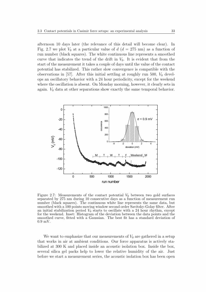
afternoon 10 days later (the relevance of this detail will become clear). InFig. 2.7 we plot V0 at a particular value of d (d = 275 nm) as a function ofrun number (black squares). The white continuous line represents a smoothedcurve that indicates the trend of the drift in V0. It is evident that from thestart of the measurement it takes a couple of days until the value of the contactpotential has stabilized. This rather slow convergence is compatible with theobservations in [57]. After this initial settling at roughly run 500, V0 devel-ops an oscillatory behavior with a 24 hour periodicity, except for the weekendwhere the oscillation is absent. On Monday morning, however, it clearly sets inagain. V0 data at other separations show exactly the same temporal behavior.
0 500 1000 1500 2000
-120
-100
-80
-60
-40
-20
0
V 0 (m
V)
run number
-4 -2 0 2 40
200
400
600
800
1000
occu
renc
e
deviation (mV)
σ = 0.9 mV
M T W T F Weekend M
Figure 2.7: Measurements of the contact potential V0 between two gold surfacesseparated by 275 nm during 10 consecutive days as a function of measurement runnumber (black squares). The continuous white line represents the same data, butsmoothed with a 100 points moving window second order Savitsky-Golay filter. Afteran initial stabilization period V0 starts to oscillate with a 24 hour rhythm, exceptfor the weekend. Inset: Histogram of the deviation between the data points and thesmoothed curve, fitted with a Gaussian. The best fit has a standard deviation of0.9 mV.
We want to emphasize that our measurements of V0 are gathered in a setupthat works in air at ambient conditions. Our force apparatus is actively sta-bilized at 300 K and placed inside an acoustic isolation box. Inside the box,several silica gel packs help to lower the relative humidity of the air. Justbefore we start a measurement series, the acoustic isolation box has been open

34 2 Calibration with the electrostatic force
for some time to allow for sample placement and AFM optical lever alignment.After closing the acoustic isolation chamber, the air inside the box is gettingwarmer (because of the heating due to the temperature stabilization system)and less humid (because of the silica gel packs). We speculate that the slowdecrease in V0 in the first couple of days is caused by a change in the thick-ness and composition of the adsorbed water films covering our surfaces, as aconsequence of the constant increase of temperature and decrease of humidity.After 2 days, the air inside the box reaches an equilibrium and the exponentialbehavior ceases.
The daily oscillation of roughly 10 mV that we observe at a later stage mustsomehow be caused by a change in the temperature of the laboratory, whichis oscillating strongly in winter (the central heating system of the building isswitched off during the nights and weekends and isolation is poor). Voltagevariations in the electrical leads and connections due to the Seebeck effect areunlikely, simply because the oscillations are too big: typical thermo-couplecoefficients are around tens of µV/K and can thus never account for morethan 1 mV of V0 oscillation. However, the variation of the temperature of thelaboratory slightly alters the temperature of the air inside the box because thebox does not provide sufficient thermal isolation. This temperature variationof the air that is in contact with the investigated surfaces might induce changesin the properties of the adsorbed water layers.
Separation dependence
In [19], we investigated the dependence of the V0 data on separation for onespecific measurement run out of a measurement series containing 184 runs. Itis interesting to analyze more deeply the data presented in [19], and assess theseparation dependence for all measurement runs. First, in Fig. 2.8, we plotV0 versus d for another, randomly chosen, single run. The straight line is thebest fit of a function V0(d) = a log(d) + b to the data, resulting in a reducedχ2 of 0.93. To understand whether we can extract some systematic propertiesof V0 from the 184 data sets, we fitted the function V0(d) = a log(d) + b toall of them. In inset a, we plot the offset fit parameter, b, as a function oftime (we have removed run 176 because it is an outlier). In this data thereis not such a strong drift in V0 with time as in Fig. 2.7, because the acousticisolation box was already closed for quite some time before the data of Fig. 2.8were gathered; the initial settling of V0 had already taken place before thefirst run. In inset b of Fig. 2.8, we plot the slope a of the fits as a functionof run number, where the error bars denote the errors on the fit parameter aspropagated through the fit procedure. It seems that a does not depend on time.If we fit a constant to these data, though, we obtain a reduced χ2 of 1.4, whichmeans that it is quite unlikely that the model is correct given the fact thatwe have 182 degrees of freedom. Therefore, we have either underestimated the

2.3 Contact potentials in Casimir force setups: an experimental analysis 35
-5.5 -5.0 -4.5 -4.00
10
20
30
40
50
60
occu
renc
e
a (mV/order of magnitude)
100 1000-14
-12
-10
-8
-6
-4
-2
V 0 (m
V)
d (nm)
0 50 100 150 200
-1012345678
b (m
V)run number
0 50 100 150 200-6.0
-5.5
-5.0
-4.5
-4.0
-3.5
a (m
V/or
der o
f mag
nitu
de)
run number
b) c)
a)
Figure 2.8: Re-analysis of the data published in [19]. The main figure shows thedistance dependence of V0 of a single measurement run from the 184 data sets of[19]. The line indicates the best fit with a logarithmic function V0(d) = a log(d) + b(reduced χ2 = 0.93, a = −4.5± 0.3 mV/order of magnitude, b = 4.6± 0.6 mV andd in nm) a, Plot of the variation in time of the fit parameter b. b, Plot of the timedependence of the fit parameter a c, Histogram of all obtained values for a. Thebest fit with a Gaussian resulted in a = −4.6± 0.6 mV.

36 2 Calibration with the electrostatic force
error on a or there is a hidden dependence of V0 on time. The first option is notreally feasible, because the reduced χ2 values of the logarithmic fits distributedneatly around 1, and the error on a is just calculated from this fit procedure.The second hypothesis would indicate that there is a dependence of a on runnumber, albeit in a random way (there is no apparent functional dependencevisible in Fig. 2.8 a). We speculate that such a random contribution to theV0 scaling properties may be related to the actual measurement procedure.Namely, during a measurement run, where we start at large separation anddecrease d in successive steps, we reduce the excitation voltage VAC to keepthe electrostatic force constant (see [19]). At the end of the run we retractthe piezoelectric stage quickly while the VAC excitation voltage is still at thelowest setting (as we were at the closest point). After a few seconds, thenext run is started and the VAC value is increased again to reach the sameelectrostatic force as we used in the run before. This procedure leads to asignificant drop in electrostatic field strength in between measurement runs.It could be that this fast change of field strength causes the adsorbed waterlayer and its contaminants to rearrange on the surfaces. Fig. 2.8 c presents allthe obtained values of a in a histogram. The Gaussian fit resulted in a valuefor a of −4.6± 0.6 mV/order of magnitude. It is interesting to note that thevalues of a follow a normal distribution, which then indicates that, althoughthere is a random run-to-run variation in a (by which we mean a real variationand not one that merely follows from the statistical uncertainties in the V0
measurements), this run-to-run randomness of a follows a normal distribution.
To complete the analysis, it is interesting to check whether the data pre-sented in Fig. 2.7 also depend on the separation between the interacting sur-faces. In order to assess the precision of our data, we have smoothed the V0
data with a second order Savitsky-Golay filter with a 100 points moving win-dow and plotted the resulting curve as the white line in Fig. 2.7. Then wehave created a histogram of the deviations between the actual data and thesmooth line and fitted a Gaussian function with the standard deviation as theonly fit parameter, as shown in the inset of Fig. 2.7. The resulting standarddeviation is 0.9 mV, which is thus the statistical error in a single V0 measure-ment at d = 275 nm. Because the loop gain of our negative feedback loopdepends on separation, the precision in the measurement of V0 is separationdependent: the precision increases when the separation decreases. Therefore,we have repeated the described procedure for 5 other values of d (covering theentire measurement range) and then fitted the size of the statistical error as afunction of separation with an exponential that seemed to describe the generaltrend well. In the continuing analysis, we can now use this fit function toobtain the statistical error in V0 at any separation within the analyzed range.
Similarly to Fig. 2.8, we plot the contact potential versus the surface sep-aration for a randomly chosen run (run 1000) on a semi-logarithmic scale inFig. 2.9. The continuous line is a fit to the data assuming a V0 = a log(d) + b
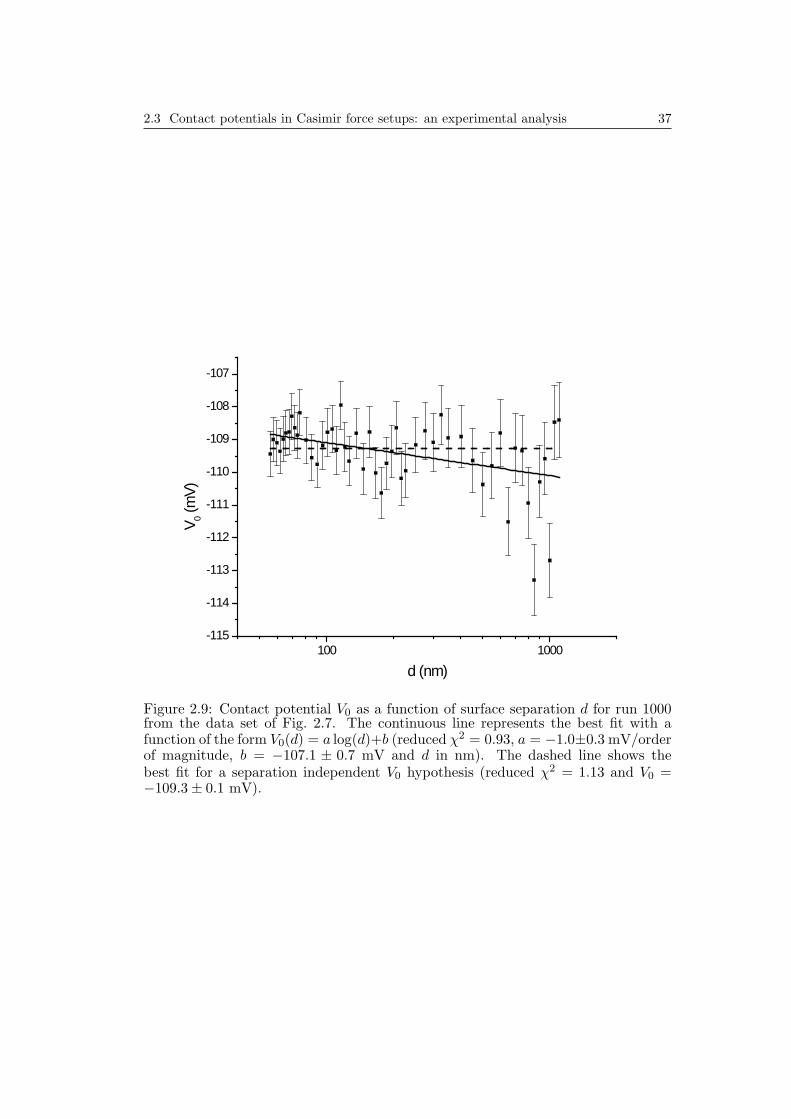
2.3 Contact potentials in Casimir force setups: an experimental analysis 37
100 1000-115
-114
-113
-112
-111
-110
-109
-108
-107
V 0 (m
V)
d (nm)
Figure 2.9: Contact potential V0 as a function of surface separation d for run 1000from the data set of Fig. 2.7. The continuous line represents the best fit with afunction of the form V0(d) = a log(d)+b (reduced χ2 = 0.93, a = −1.0±0.3 mV/orderof magnitude, b = −107.1 ± 0.7 mV and d in nm). The dashed line shows thebest fit for a separation independent V0 hypothesis (reduced χ2 = 1.13 and V0 =−109.3± 0.1 mV).

38 2 Calibration with the electrostatic force
functional dependence (reduced χ2 = 0.93), whereas the dashed line assumessimply a constant contact potential (reduced χ2 = 1.13). Although the re-duced χ2 values of both fits are quite close to 1, one can see by eye that theresiduals related to the dashed fit show a systematic behavior for large d, in-dicating that a constant contact potential does not model the data well. Theresiduals belonging to the log(d) behavior are clearly more random, but itwould be quite bold to claim that the model is correct. A better formulationwould be to state that with the relatively big statistical error compared to thetotal variation of V0 in Fig. 2.9, we cannot exclude the logarithmic dependenceon separation.
100 1000-109.4
-109.2
-109.0
-108.8
-108.6
-108.4
-108.2
V 0 (m
V)
d (nm)
Figure 2.10: Contact potential V0 as a function of surface separation d, obtained byaveraging all but the first 250 runs from the data set of Fig. 2.7.
It is thus clear that an improvement in the precision of V0 could lead tomore conclusive statements regarding its dependence on separation. Since thedata were acquired during more than a week, there is ample room to employaveraging procedures. We have therefore averaged the last 1694 measurementruns and plotted the resulting mean V0 values in Fig. 2.10. We have excludedthe first 250 runs from the averaging procedure because of their strong drift(see Fig. 2.7). Although the total variation in V0 is of course still small at alittle less than 1 mV, the high precision in the mean values of V0 reveals adefinite trend in the data∗∗. For d > 100 nm, V0 seems to scale logarithmically
∗∗In this experiement, GL varies from 4.3 103 at d = 1 µm to 1.6 104 at d = 60 nm.

2.3 Contact potentials in Casimir force setups: an experimental analysis 39
with separation, in agreement with the observations in [38] and [19]. Ford < 100 nm, however, the trend is clearly altered. We would therefore like toconclude that in these experiments there is certainly a logarithmic contributionin the function V0(d), but there are definitely other components too.
2.3.4 Conclusions
We have reported systematic measurements of the contact potential differencebetween a gold coated sphere and a gold coated plate kept in air at sub-micronseparation. Our data confirm that the contact potential in Casimir force ex-periments can depend on both separation and time, and seem to indicate thatwater layers on the interacting surfaces play an important role in the electro-static interaction between conducting surfaces in ambient conditions. We hopethat our findings will trigger new theoretical investigations on the behavior ofcontact potentials in Casimir force experiments.
Acknowledgments
The authors thank J. H. Rector, F. Mul, and R. Griessen for useful discussions,and the ESF Research Network CASIMIR for providing visit grants. Thiswork was supported by the Netherlands Organisation for Scientific Research(NWO), under the Innovational Research Incentives Scheme VIDI-680-47-209.D.I. acknowledges financial support from the European Research Council un-der the European Community’s Seventh Framework Programme (FP7/2007-2013)/ERC grant agreement 201739.
Therefore, the systematic error in V0 varies from < 12 µV to < 3 µV with |VDC | < 50 mV(see Eq. 2.14). The effect of this systematic error can thus at most be a tilt in the data of±9 µV over the whole d range, which is still negligible compared to the observed variationin V0.

Chapter 3
Halving the Casimir force
3.1 Introduction
The strength of the Casimir interaction depends only on the separation be-tween the objects and the dielectric properties of their surfaces and the inter-vening medium. As long a one does not work in liquids, the dielectric proper-ties of the medium are essentially equal to those of vacuum, and one can onlyalter the interaction strength by tuning the material properties. To weakenthe force, one has to use material properties that do not impose such strongboundary conditions on the electromagnetic quantum fluctuations in the gap.It is thus necessary to use materials that are not electrically conductive overa wide part of the electromagnetic spectrum. On the other hand, however, itwould not make much sense to use insulators, because, although the Casimirforce is supposed to be small, electric forces generated by trapped charges onthe surfaces would be so strong that the total force between the objects wouldbe much larger than the Casimir force between metals. Therefore, an idealmaterial would be DC conductive enough to prevent charge accumulation, buttransparent enough for infrared and optical frequencies to significantly reducethe Casimir interaction. In section 3.2 we describe an experiment that showsthat by using a transparent conductive oxide, typically used for touch screensin semiconductor industry, one can halve the Casimir force with respect to thegold-gold interaction.
In section 3.3, we expand the description of the experiment presented insection 3.2, and discuss in full detail the experimental technique and charac-terization of the samples. This section also treats the experimental errors anddata analysis, as well as a new method to determine the spring constant of theforce sensor using the fourth harmonic of the electrostatic excitation voltageat ω1. This section is the most complete description of our experimental setup,and can be used as a reference for future use. Concerning the experimentaldetails of the residual potential compensation circuit, the best description isin section 2.3.
40
3.2 Halving the Casimir force with Conductive Oxides 41
3.2 Halving the Casimir force with Conduc-tive Oxides
Abstract – The possibility to modify the strength of the Casimir effect bytailoring the dielectric functions of the interacting surfaces is regarded as aunique opportunity in the development of Micro- and NanoElectroMechanicalSystems. In air, however, one expects that, unless noble metals are used,the electrostatic force arising from trapped charges overcomes the Casimirattraction, leaving no room for exploitation of Casimir force engineering atambient conditions. Here we show that, in the presence of a conductive oxide,the Casimir force can be the dominant interaction even in air, and that theuse of conductive oxides allows one to reduce the Casimir force up to a factorof 2 when compared to noble metals.
This paper has been published: S. de Man, K. Heeck, R. J. Wijngaarden, and D. Ian-nuzzi, Phys. Rev. Lett. 103, 040402 (2009). It was highlighted in P. Ball, News and Views,Nature Materials 8, 705 (2009).

42 3 Halving the Casimir force
The mechanical parts of Micro- and NanoElectroMechanical Systems (MEMSand NEMS) are often designed to work at separations where the Casimir ef-fect [18] might play a relevant role [1–4]. It is thus commonly believed that, ifone could suitably engineer the strength of the Casimir force, unprecedentedopportunities would come available for the development of conceptually newMEMS and NEMS [5–7, 14]. The most simple approach to tailor the Casimirforce is to properly choose the materials of which the interacting surfaces aremade. According to the Lifshitz theory [23], the interaction between two ob-jects depends on their dielectric functions. Transparent dielectrics, for exam-ple, attract less than reflective mirrors. This property may be used to reducethe Casimir attraction whenever the design requires a smaller short range in-teraction. It is however fair to say that, for the vast majority of applications,MEMS and NEMS operate in air, where surfaces tend to accumulate trappedcharges. Those charges give rise to a strong electrostatic interaction that can-not be compensated by a counterbias voltage and that typically overcomes theCasimir force. It is thus difficult to imagine that the Casimir force can play animportant role in MEMS and NEMS operating in air, unless all surfaces arecoated with noble metals to reduce the forces due to surface charges to negligi-ble levels. In that case, however, there is not much room to tune the strengthof the Casimir interaction because the diversity in the dielectric functions ofdifferent metals is simply not large enough [30]∗. As a matter of fact, to date,there is no experiment that shows that, in air, the Casimir force can still betuned significantly while remaining the dominant interaction mechanism.
In this Letter we present a precise measurement of the Casimir force be-tween a gold coated sphere and a glass plate coated with either a thick goldlayer or a highly conductive, transparent oxide film. The experiment was per-formed in air, and no electrostatic force due to residual trapped charges wasobserved over several weeks of measurements in either case. The decrease ofthe Casimir force due to the different dielectric properties of the reflective goldlayer and the transparent oxide film resulted to be as high as ' 40% − 50%at all separations (from ' 50 to ' 150 nm). Our experiment shows that, inthe presence of a conductive oxide layer, the Casimir force can still be thedominant interaction mechanism even in air, and indicates that, whenever thedesign might require it, it is possible to tune the Casimir attraction by a factorof 2.
Our experimental set-up is designed to perform precise measurements ofsurface forces between a 100 µm radius sphere and a plate as a function of theirseparation (see Fig. 3.1 and [19]). The sphere is glued onto the hanging end
∗An unsuccesful attempt to change the Casimir force in gas is reported in [32]. ' 1%tunability of the Casimir force in vacuum was shown in [60]. ' 20% tunability of theCasimir force was observed in [33]; this method is not practical, because the interactionstrength strongly varies on the local thickness of the film (see [36]). ' 30% variations ofthe Casimir force were observed in [61]; also this strategy is not practical for MEMS in air,because the passivation layer is not stable under atmospheric conditions.

3.2 Halving the Casimir force with Conductive Oxides 43
Alu
min
um h
eat r
eser
voir
Commercial AFM head
quadrantphotodetector
VDC
VAC
Data storage
(a) (b)
Initial position Generic position
interactingsurfaces
Custom-designedmechanical translators
piezoelectric transducers
V0 feedback circuit
Calibration lock-in
Measurement lock-in
d0dpz
d
(c)
Figure 3.1: a, Drawing of the experimental set-up. b, Schematic representationof the working principle of the experimental technique. c, Definition of d0 (initialseparation), dpz (movement of the piezoelectric stage), and d (separation betweenthe two surfaces).

44 3 Halving the Casimir force
of a micromachined cantilever (spring constant ≈ 1 N/m, resonance frequency(with the sphere attached) ≈ 1.9 kHz). The plate is mounted on a capacitivefeedback controlled piezoelectric transducer that allows one to accurately varythe separation between the sphere and the plate in discrete steps. Any forceacting between the two surfaces results in a bending of the cantilever that isdetected by the optical lever of a commercial Atomic Force Microscope (AFM)head †. The set-up is kept at a fixed temperature to reduce mechanical driftsand is placed on an active anti-vibration stage inside an acoustic isolation boxto decouple the force sensor from external vibrations.
Precise Casimir force measurements typically require careful analysis ofthree crucial issues. First, even when both the sphere and the plate are coatedwith metallic films, there might still exist an electrostatic potential differenceV0 between the two surfaces that gives rise to a residual electrostatic force. Thisforce must be actively canceled by counter biasing V0 with an externally ap-plied voltage. Second, although the relative displacements of the piezoelectrictransducer that moves the plate, dpz, are precisely controlled, the separationbetween the two interacting surfaces at the start of the measurement, d0, is apriori unknown (see Fig. 3.1). Therefore, the absolute separation d = d0−dpzhas to be obtained from a calibration procedure. Third, the electronic signalcoming out of the AFM head must be converted into force. It is thus nec-essary to calibrate the instrument with a controlled force. To address theseproblems, we have designed a measurement technique that allows one to simul-taneously: (i) compensate for the residual potential, (ii) calibrate the set-up,and (iii) measure the Casimir force (see [19] and section 3.3). In a nutshell,in each calibration/measurement run the plate is moved in discrete steps fromd0 to a minimum value of d (just before contact with the sphere). A cali-brated AC electrostatic potential is applied between the sphere and the plateat a frequency ω1 much lower than the resonance frequency of the force sensor(ω1
2π= 72.2 Hz). This AC excitation is used to drive a feedback circuit that
compensates for the residual voltage V0, and, simultaneously, generates an elec-trostatic force that makes the cantilever oscillate at 2ω1. The amplitude of theoscillations, measured with a lock-in amplifier (calibration lock-in in Fig. 3.1b),are recorded as a function of dpz, and are then used to calibrate the instrumentand extract d0. At the same time, a transducer mechanically coupled to thepiezoelectric translator makes the plate move around dpz with an amplitude of3.85 ± 0.08 nm at a frequency ω2, which is again much lower than the reso-nance frequency of the force sensor (ω2
2π= 119 Hz) ‡. In the presence of a force
that depends on separation (e.g., the Casimir force), the cantilever bends inphase with the modulation of d. The amplitude of the in-phase oscillation,
†Measurements of surface forces between a sphere and a plate with an AFM were firstreported in [34]. Its utilisation for large range forces between metals was first introduced in[35].‡A similar technique was introduced in [62].

3.2 Halving the Casimir force with Conductive Oxides 45
measured with another lock-in amplifier (measurement lock-in in Fig. 3.1b), isproportional to the derivative of the force with respect to d. Furthermore, thepresence of the cushion of air between the two surfaces gives rise to a hydro-dynamic force that depends on the velocity with which the plate moves. Thesignal produced by this force manifests itself at the same frequency at whichd is modulated, but with a phase rotated by 90 degrees. This contributiondoes not influence the output of the in-phase component and can be measuredindependently with the same lock-in amplifier. The integration times of thelock-in amplifiers are 8 s for every value of dpz. A typical measurement runconsists of ' 50 dpz set-points in the measurement range 50 < d < 1100 nm,and takes roughly 7 minutes. The cantilever responses to the modulations atω1 and ω2 are < 80 pm (root-mean-square) during the entire experiment. Allforce measurements are performed in air at atmospheric pressure, temperature300 K, and 29% relative humidity.
In this Letter we present two experiments performed with the same sphereand two different plates. The sphere is a polystyrene sphere with nominalradius 100 µm coated with a Ti adhesion layer followed by a 100 nm Au film(surface roughness 3.8 nm RMS). The plate used in the first experiment isa polished sapphire substrate coated with a metallic film similar to the onedeposited on the sphere (surface rougness 0.8 nm RMS). The plate used inthe second experiment is a float glass substrate with a 190 nm Indium TinOxide (ITO, In2O3:Sn) sputtered thin film on top (PGO CEC010S, typically8.5 Ω/, or, equivalently, ρ = 1.6 10−4 Ωcm, total surface roughness 4 nmRMS). We have measured the reflection and transmission spectra of both platesin the wavelength range 180 nm < λ < 2.5 µm, and observed that the opticalproperties of our films are in agreement with the literature [63, 64].
Fig. 3.2a presents measurements of the force between the sphere and theplates coated with either Au or ITO §. The experimental data represent thespatial derivative of the total force (normalized by the sphere radius R), whichis the sum of the Casimir interaction, a Coulomb interaction induced by thepresence of trapped charges (if any), and an electrostatic attraction due to theAC calibration potential. The strength of the latter can be estimated fromthe simultaneous calibration procedure (see section 3.3). From Fig. 3.2, it isevident that this electrostatic contribution, which is anyway equal in both ex-periments (within 2%), is small compared to the total force signal. The blacklines in Fig. 3.2a are computations of the Casimir force using the Lifshitz the-ory [41] with dielectric functions calculated as in [64] (for ITO) and [65] (forAu); the electrostatic force due to the calibration potential is added to thetheory in order to compare with the raw data. The calculation of the Casimir
§Our estimate of d0 relies on the proximity force approximation [41], which is only validfor d R. This assumption is not entirely correct in the probed separation range [19]and results in a systematic error in d0 of ' 1.4 nm. Still, the corresponding underestimateof the separation is equal for both Au-Au and Au-ITO, and can thus be neglected in thecomparison.

46 3 Halving the Casimir force
60 80 100 120 140 160 180 2000
100
200
300
400
500
d (nm)
60 80 100 120 140 160 180 2001
10
100
d (nm)
5 10 15 20 25
40 50 60 70 80 90
a b c
d
~ 40%
~ 50%
Figure 3.2: a, Spatial derivative of the total force as a function of absolute surfaceseparation for the Au-Au (green squares) and Au-ITO (red squares) interactionsfor randomly chosen subsets of the data (150 out of 580 for both cases). The blueline represents the derivative of the electrostatic force caused by the simultaneouscalibration procedure (common to both the gold and ITO measurements). Theblack lines indicate the calculated Casimir forces with the electrostatic backgroundadded. b, Spatial derivative of the Casimir force, with the electrostatic backgroundsubtracted from the data. The black lines correspond to the calculations of theCasimir force. c, Histograms of 580 force measurements for Au-Au and Au-ITO atd = 120 nm. d, Same as c, but for d = 80 nm.

3.2 Halving the Casimir force with Conductive Oxides 47
force should only be considered approximate, because the dielectric functionsof the samples are not known precisely [66], and no surface roughness correc-tions are applied. Still, the agreement between the calculation and the datashows that the Casimir effect largely dominates any Coulomb interaction thatwould have been otherwise observed in the presence of a significant amount oftrapped charges. Fig. 3.2b shows the data and theory on a double logarithmicscale, where we have subtracted the electrostatic background due to the ACcalibration potential using the simultaneously obtained calibration data. Atsmall separations d < 60 nm, both data sets curve upwards, which might be asign of surface roughness effects. At separations d > 120 nm, the experimentaldata for the Au-Au Casimir interaction start to deviate significantly from thetheory because of an artefact caused by reflections from the optical lever lightby the sample. This reflected light reaches the photodetector and causes abackground signal that is not related to any force. This artefact is commonto all optical lever based AFM techniques, and the related signal is typicallyassumed to be linear in the piezo extension and subtracted from the data ac-cordingly [35]. Because the reflectivities of our two samples are so different,we prefer to refrain from such a procedure, and present the data as is. InFigs. 3.2c and d we show histograms of all the obtained measurements for thederivative of the Casimir force for two specific separations (d = 120 nm andd = 80 nm). The histograms at d = 80 nm can be described by Gaussians witha standard deviation of roughly 5%, which means that our method provides aprecision in the mean measured Casimir force derivative of 0.2%. It is evidentfrom the histograms that the spatial derivative of the Casimir force between aAu and an ITO surface is roughly ' 40%− 50% smaller than between two Ausurfaces. In our geometry (i.e., for separations much smaller than the radius ofthe sphere), the spatial derivative of the force is proportional to the pressurebetween two parallel plates [41]. We can thus conclude that the Casimir pres-sure that one would measure between a Au plate kept parallel to an ITO platewould be roughly ' 40%− 50% smaller than in the case of two Au plates.
Even though the agreement between the theoretical prediction and themeasurement of the Casimir force in both situations is good, one might stillargue that the observed decrease could be mimicked by drifts in d0. For bothmeasurements series, we gathered 580 data sets continuously, which allows usto directly assess the run-to-run drift of d0. Due to the temperature stabiliza-tion of our setup, the mechanical drift is very small at ' 0.1 nm and ' 0.2 nmper run for the Au-Au and the Au-ITO experiments, respectively. We con-clude that the decrease of the Casimir force cannot be ascribed to drifts ind0. We have also verified that the electrostatic force used to calibrate the in-strument and extract d0 follows what expected from elementary electrostaticarguments, as suggested in [38] and discussed in [19]. Concerning the com-pensation voltage, we observed that V0 varies approximately 1 mV and 3 mVover the complete measurement range in the Au-Au and Au-ITO cases, respec-

48 3 Halving the Casimir force
tively ¶. These slight variations of V0 do not compromise the measurement ofthe Casimir force at the current level of sensitivity.
Finally, the different surface roughnesses of the sphere and the plates alsoinfluence the strength of the Casimir effect. Since both experiments are con-ducted with the same sphere, the difference in the observed Casimir force cannever be due to the surface roughness of the sphere. Second, we recall thatthe surface roughness of the ITO sample is larger than that of the Au sub-strate. Since surface roughness enhances the Casimir force [67] we note that,if it played a role in the probed separation range, it would lead to a strongerinteraction between Au and ITO than between two Au surfaces, contrary tothe measurements presented in Fig. 3.2.
100 1000
100
200
300
400
500
d (nm)
Figure 3.3: Hydrodynamic force acting on the sphere as a function of the absoluteseparation d for Au-Au (green squares) and Au-ITO (red squares), for the data setsshown in Figs. 3.2a and b.
To make our claim even more robust, we can now compare the hydrody-namic force observed during the two experiments. Because the geometricalconfiguration of the experiment is equal in both cases, we expect to measurethe same hydrodynamic force. The results are shown in Fig. 3.3. It is clearthat the hydrodynamic force is very similar in both cases, although there ex-ists a slight discrepancy between the two curves (' 2%). Since both curves
¶The value of V0 at d = 100 nm during the entire experiment drifts from −106 mV to−103 mV for Au and from 72 mV to 50 mV for ITO.

3.2 Halving the Casimir force with Conductive Oxides 49
are parallel on a double logarithmic scale, we conclude that this discrepancycannot be ascribed to a difference in the calibration of d0. Therefore, we ruleout that the large difference in the Casimir force reported in Fig. 3.2 be dueto an error in the determination of d0.
In conclusion, we have demonstrated that an ITO coating of one of thetwo surfaces is sufficient to readily create situations where the Casimir force isstill the dominant interaction mechanism regardless the presence of air in thesurroundings. Since ITO is transparent over a wide range of frequencies, theCasimir attraction is up to a factor of 2 smaller when compared to the case ofthe Au-Au interaction, leaving ample room for Casimir force engineering evenat ambient conditions, where MEMS and NEMS typically operate.
This work was supported by the Netherlands Organisation for ScientificResearch (NWO), under the Innovational Research Incentives Scheme VIDI-680-47-209. The authors thank A. Baldi, F. Mul, U. Mohideen, J. H. Rec-tor, B. Dam, and R. Griessen for useful discussions, and the ESF ResearchNetwork CASIMIR for providing visit grants. S. M. acknowledges financialsupport from the Kavli Institute for Theoretical Physics (NSF PHY05-51164).D.I. acknowledges financial support from the European Research Council un-der the European Community’s Seventh Framework Programme (FP7/2007-2013)/ERC grant agreement 201739.
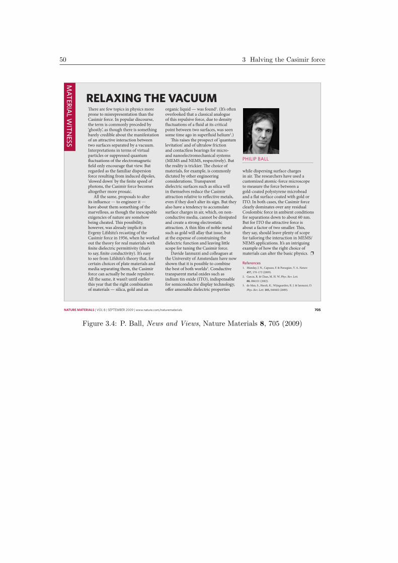
50 3 Halving the Casimir force
nature materials | VOL 8 | SEPTEMBER 2009 | www.nature.com/naturematerials 705
news & views
and making them accessible for catalysis (Fig. 1b,c). The hydrolysis reaction can be followed by the emerging fluorescence of the hydrolysed FDP.
The process of masking and unmasking the enzymes is reversible, and thus bioactivation can be turned on or off on demand by applying more or less mechanical strain. When the film is no longer stretched, the enzymes are again masked by the dense polymer barrier and the catalysis is switched off.
The researchers identified two important requirements needed for successful mechanically tunable enzymatic reactions. First, the barrier should be thick enough to prevent enzyme diffusion through the unstretched barrier, but at the same time it should be relatively thin to unmask the enzyme on stretching. Second, the
critical stretching degree required for the biocatalytic activation was found to be 70%, a significant level of deformation.
The work of Voegel and co-workers shows that the design of ‘cryptic-like’ surfaces capable of reversibly inducing biochemical reactions by applying a mechanical stress is feasible with layer-by-layer materials. Manipulating the construct design, for example, by varying the barrier thickness and reservoir parameters, is a way to tune the amplitude of the biocatalytic activity triggered by mechanical stimuli. The work has great potential in the design of responsive bioengineered materials aimed at triggering and modulating chemical and biochemical reactions by mechanical action, with applications ranging from smart microbiofluidic devices to mechanically controlled biopatches.
Eugenia Kharlampieva and Vladimir V. Tsukruk are at the School of Materials Science and Engineering, Georgia Institute of Technology, Atlanta, Georgia 30332, USA. e‑mail: [email protected]
References1. Luzinov, I., Minko, S. & Tsukruk, V. V. Prog. Polym. Sci.
29, 635–698 (2004). 2. Mertz, D. et al. Nature Mater. 8, 731–735 (2009).3. Decher, G. & Schlenoff, J. B. (eds) Multilayer Thin Films: Sequential
Assembly of Nanocomposite Materials (Wiley-VCH, 2003).4. Jiang, C. & Tsukruk, V. V. Adv. Mater. 18, 829–840 (2006).5. Srivastava, S. & Kotov, N. Acc. Chem. Res. 41, 1831–1841 (2008).6. Hiller, J., Mendelsohn, J. D. & Rubner, M. F. Nature Mater.
1, 59–63 (2002).7. Lvov, Y. & Caruso, F. Anal. Chem. 73, 4212–4217 (2001).8. Kharlampieva, E. & Sukhishvili, S. J. Macromol. Sci.‑Polym. Rev.
46, 377–395 (2006).9. Sukhorukov, G. B. & Möhwald, H. Trends Biotechnol.
25, 93–98 (2007).10. Genzer, J. & Efimenko, K. Science 290, 2130–2133 (2000).11. Betanzos, M., Chiang, C. S., Guy, H. R. & Sukharev, S.
Nature Struct. Biol. 9, 704–710 (2002).
MaTeRia
l wiTn
ess
There are few topics in physics more prone to misrepresentation than the Casimir force. In popular discourse, the term is commonly preceded by ‘ghostly’, as though there is something barely credible about the manifestation of an attractive interaction between two surfaces separated by a vacuum. Interpretations in terms of virtual particles or suppressed quantum fluctuations of the electromagnetic field only encourage that view. But regarded as the familiar dispersion force resulting from induced dipoles, ‘slowed down’ by the finite speed of photons, the Casimir force becomes altogether more prosaic.
All the same, proposals to alter its influence — to engineer it — have about them something of the marvellous, as though the inescapable exigencies of nature are somehow being cheated. This possibility, however, was already implicit in Evgeny Lifshitz’s recasting of the Casimir force in 1956, when he worked out the theory for real materials with finite dielectric permittivity (that’s to say, finite conductivity). It’s easy to see from Lifshitz’s theory that, for certain choices of plate materials and media separating them, the Casimir force can actually be made repulsive. All the same, it wasn’t until earlier this year that the right combination of materials — silica, gold and an
organic liquid — was found1. (It’s often overlooked that a classical analogue of this repulsive force, due to density fluctuations of a fluid at its critical point between two surfaces, was seen some time ago in superfluid helium2.)
This raises the prospect of ‘quantum levitation’ and of ultralow friction and contactless bearings for micro- and nanoelectromechanical systems (MEMS and NEMS, respectively). But the reality is trickier. The choice of materials, for example, is commonly dictated by other engineering considerations. Transparent dielectric surfaces such as silica will in themselves reduce the Casimir attraction relative to reflective metals, even if they don’t alter its sign. But they also have a tendency to accumulate surface charges in air, which, on non-conductive media, cannot be dissipated and create a strong electrostatic attraction. A thin film of noble metal such as gold will allay that issue, but at the expense of constraining the dielectric function and leaving little scope for tuning the Casimir force.
Davide Iannuzzi and colleagues at the University of Amsterdam have now shown that it is possible to combine the best of both worlds3. Conductive transparent metal oxides such as indium tin oxide (ITO), indispensable for semiconductor display technology, offer amenable dielectric properties
while dispersing surface charges in air. The researchers have used a customized atomic-force microscope to measure the force between a gold-coated polystyrene microbead and a flat surface coated with gold or ITO. In both cases, the Casimir force clearly dominates over any residual Coulombic force in ambient conditions for separations down to about 60 nm. But for ITO the attractive force is about a factor of two smaller. This, they say, should leave plenty of scope for tailoring the interaction in MEMS/NEMS applications. It’s an intriguing example of how the right choice of materials can alter the basic physics.
References1. Munday, J. N., Capasso, F. & Parsegian, V. A. Nature
457, 170–173 (2009).2. Garcia, R. & Chan, M. H. W. Phys. Rev. Lett.
88, 086101 (2002).3. de Man, S., Heeck, K., Wijngaarden, R. J. & Iannuzzi, D.
Phys. Rev. Lett. 103, 040402 (2009).
Relaxing the vacuum
PhILIP BALL
nmat_N&V_SEP09.indd 705 11/8/09 09:27:52
© 2009 Macmillan Publishers Limited. All rights reserved
Figure 3.4: P. Ball, News and Views, Nature Materials 8, 705 (2009)

3.3 Halving the Casimir force with conductive oxides: experimental details 51
3.3 Halving the Casimir force with conductiveoxides: experimental details
Abstract – This work is an extended version of a paper published last yearin Physical Review Letters [S. de Man et al., Phys. Rev. Lett. 103, 040402(2009)], where we presented measurements of the Casimir force between agold coated sphere and a plate coated with either gold or an indium-tin-oxide(ITO) layer. The experiment, which was performed in air, showed that ITOis sufficiently conducting to prevent charge accumulation, but still transpar-ent enough to halve the Casimir attraction when compared to gold. Here,we report all the experimental details that, due to the limited space avail-able, were omitted in the previous article. We discuss the performance of oursetup in terms of stability of the calibration procedure and reproducibility ofthe Casimir force measurement. We also introduce and demonstrate a newtechnique to obtain the spring constant of our force sensor. Furthermore, wepresent a thorough description of the experimental method, a comprehensiveexplanation of data elaboration and error analysis, and a complete character-ization of the dielectric function and of the surface roughness of the samplesused in the actual experiment.
¶This paper has been published: S. de Man, K. Heeck, and D. Iannuzzi, Phys. Rev. A82, 062512 (2010)

52 3 Halving the Casimir force
3.3.1 Introduction
It is well known that the Casimir effect [18] strongly depends on the dielectricfunction of the interacting surfaces [23, 41]. Transparent dielectrics, for exam-ple, attract less than highly reflective metals. Dielectric materials, however,tend to accumulate isolated charges. Those charges give rise to an electrostaticforce that easily overcomes the Casimir interaction.
In a recent paper [20], we have presented measurements of the Casimir forcebetween a gold coated sphere and a plate coated with either gold or an Indium-Tin-Oxide (ITO, In2O3:Sn) layer. The experiment, which was performed inair, showed that ITO is sufficiently conducting to prevent charge accumulation,but still transparent enough to halve the Casimir attraction when comparedto gold.
The experiment was carried out by means of a quite complicated novel tech-nique that, due to the limited space available, was not thoroughly explainedin our previous work. We believe it is important to extend that work andprovide the community with all the details of the experimental technique anddata analysis, which is the purpose of this paper.
This paper is organized as follows. First, we describe the experimentalsetup and discuss general issues one has to tackle to perform Casimir forcemeasurements. Then we discuss the experimental technique we developed tosimultaneously calibrate the setup and measure the Casimir force gradient,and derive in detail the specific forms of all our calibration and measurementsignals. Second, we illustrate a new method to determine the spring constantof our force sensor. Third, we present experimental results on the generalperformance of our setup, namely the stability of the calibration procedure,the reproducibility of the force gradient measurements, and the spring constantdetermination. Fourth, we present the Casimir force measurements for thegold-gold and gold-ITO interactions, and show measurements of the dielectricfunctions and surface topographies of our surfaces. Finally we compare thehydrodynamic forces for the two sets of experiments.
3.3.2 Experimental setup
Description
Our experimental setup is designed to precisely measure surface forces betweena 100 µm radius sphere and planar samples at ambient pressure. The sphere isattached to a micromachined cantilever (spring constant roughly 1 N/m) whosedeflection in response to external forces can be measured with pm sensitivityby a commercial Atomic Force Microscope (AFM) detection head (Veeco Mul-timode); the detection system is formed by a laser beam that reflects fromthe free end of the cantilever and hits a position sensitive photodetector (seeFig. 3.5). The sphere-cantilever assembly is coated with a Ti adhesion layer

3.3 Halving the Casimir force with conductive oxides: experimental details 53
and a 100 nm Au film. The planar sample is mounted on a two-stage me-chanical translator formed by a stick-slip piezoelectric motor (Attocube) anda feedback controlled piezoelectric transducer (Physik Instrumente) to vary theseparation between the sphere and plate surfaces. The stick-slip motor is usedfor coarse approach (travel range 6mm), while the feedback controlled trans-ducer executes the fine distance scanning (range 12 µm, closed loop resolution50 pm). Both the detection head and the two-stage mechanical translator areanchored to a 10 cm3 Al block that is actively temperature stabilized at 300 Kto reduce mechanical drift from differential thermal expansion of the compo-nents. The Al block is screwed onto an active anti-vibration table (Halcyonics),which is placed inside an anechoic chamber. This chamber lies onto a heavymarble optical table that is located in a temperature controlled laboratory.
Three crucial issues
In a Casimir force measurement, there are three crucial issues that have to bedealt with.
First, even if one would electrically connect both interacting surfaces, thereexists an electrostatic potential difference V0 due to the different work functionsof the surfaces. Since work functions of surfaces depend on quite a number ofparameters, like crystal growth orientation and adsorbates, typically there evenexists a potential difference between surfaces made out of the same material.This electrostatic potential difference gives rise to a force that is generallystronger than the Casimir force. To avoid this problem, most Casimir forcesetups rely on a counterbias circuit that is used to apply −V0 to the surfacesin order to have no residual electrostatic force.
Second, even in setups where the distance between the sphere and theplate is varied with a feedback controlled piezoelectric transducer, one has onlyknowledge of the relative position changes and not of the absolute separationbetween the surfaces. It is thus mandatory to find the initial separation d0 witha calibration procedure. Because the distance dependence of the electrostaticforce between a sphere and a plate is known exactly, most modern setups usethis force to extract d0.
Third, the instrument has to be calibrated with a known force. Again, onecan use the electrostatic interaction to calibrate photodetector voltage versusforce. We have developed a measurement scheme that solves all three issuesat the same time.
Force modulation measurements
We present a measurement technique that makes use of simultaneous detectionof both calibration signals (based on the electrostatic force) and the Casimirforce. The motivation for this approach is the benefit of absolute certainty thatthe calibration parameters always correspond to the measured forces because

54 3 Halving the Casimir force
Alu
min
um h
eat r
eser
voir
Commercial AFM head
quadrantphotodetector
VDC
VAC
Data storage
(a) (b)
Initial position Generic position
interactingsurfaces
Custom-designedmechanical translators
piezoelectric transducers
V0 feedback circuit
Calibration lock-in
Measurement lock-in
d0dpz
d
(c)
Figure 3.5: a, Drawing of the experimental setup used to perform precise measure-ments of the Casimir force between a 100 µm radius sphere and a plate. The alu-minum block acts as a heat reservoir to keep the temperature of the setup constant.The instrument is based on a commercial AFM head that is, together with a custom-designed mechanical translator, mounted on the aluminum block. b, Schematic rep-resentation of the working principle of the experimental technique. The V0 feedbackcircuit allows one to measure and compensate the residual voltage present betweenthe sphere and the plate. The calibration lock-in amplifier is used to calibrate theinstrument and to find the initial separation between the two surfaces d0. The mea-surement lock-in amplifier performs the measurements of the Casimir force gradientand the hydrodynamic force. c, Definition of the initial separation d0, the movementof the feedback controlled piezoelectric stage dpz, and the non-modulated separationbetween the surfaces d = d0 − dpz as used in the Taylor expansion that leads toEqs. 3.2 to 3.7.

3.3 Halving the Casimir force with conductive oxides: experimental details 55
they are acquired simultaneously; it is thus impossible to have inconsistentcalibration and force data due to time-related drifts or other events. In orderto achieve this goal, we have separated the calibration and Casimir signals infrequency space: the signals are modulated at distinct frequencies that can bede-modulated individually with lock-in amplifiers.
Modulating an electrostatic interaction is extremely easy: one just has toapply a time-dependent potential difference to the sphere and the plate (VACin Fig. 3.5 b). We thus apply an oscillating voltage VDC + VAC cos (ω1t) be-tween the sphere and the plate, where VDC is used to compensate for thecontact potential difference V0 [19]. Unfortunately, modulating the Casimirforce is a lot more challenging as its strength depends only on geometryand dielectric properties of the surfaces. On the other hand, of course, thestrong distance dependence of the Casimir force can be used to modulateits strength considerably. Therefore, we chose to add a small modulationof the form ∆d cos (ω2t) to the piezoelectric transducer displacement dpz, aspreviously introduced in [62]. When the sphere and plate surfaces are sep-arated by a distance d, we have the following three forces acting on thesphere: F (V, d, ω2,∆d) = FE(V, d) + FC(d) + FH(d, ω2,∆d) where FE(V, d)is the electrostatic force for externally applied potential difference V , FC(d)is the Casimir force, and FH(d, ω2,∆d) is the hydrodynamic force due to themoving air caused by the oscillatory motion of the plate. These forces induce abending of the cantilever F/k according to Hooke’s law, where k is the springconstant of the cantilever. The output of the optical lever read-out S is thenchanged by ∆S = γF/k, where the sensitivity of the read-out is characterizedby the calibration factor γ. We will now develop the full form of this signal∆S.
Following elementary electrostatic arguments, one can show that the elec-trostatic force between a plane and a sphere of radius R is given by
FE(V, d) = −ε0πR (V + V0)2
d, (3.1)
where ε0 is the permittivity of vacuum, V is the externally applied voltage,V0 is the contact potential difference between the two surfaces, and d R(i. e. within the proximity force approximation (PFA) [41]). To evaluate thetotal signal ∆S, we substitute V = VDC + VAC cos (ω1t) and incorporate thedistance modulation ∆d cos (ω2t). We then approximate the photodetector sig-nal with a first order Taylor expansion for small excursion ∆d cos (ω2t) aroundd = d0 − dpz (see Fig. 3.5 c):
∆S(t) ' S0+Sω1 cos(ω1t)+S2ω1 cos(2ω1t)+SIω2cos(ω2t)+SQω2
sin(ω2t)+Srem(t),(3.2)
where

56 3 Halving the Casimir force
S0 = −γε0πR[(V0 + VDC)2 + V 2
AC/2]
k (d0 − dpz) +γ
kFC (d0 − dpz) , (3.3)
Sω1 = −2γε0πR (V0 + VDC)VACk (d0 − dpz) , (3.4)
S2ω1 = − γε0πR
k (d0 − dpz)V 2AC
2, (3.5)
SIω2= −γε0πR
[(V0 + VDC)2 + V 2
AC/2]
∆d
k (d0 − dpz)2 − γ
k
∂FC∂d
∣∣∣∣d0−dpz
∆d, (3.6)
SQω2=γ
kFH(d0 − dpz, ω2,∆d), (3.7)
FC (d0 − dpz) is the Casimir force at separation d0 − dpz, Srem(t) contains thecross terms at frequencies like ω1 ± ω2 and 2ω1 ± ω2 and the gradient of thehydrodynamic force at 2ω2, and we have neglected the effect of the cantileverdeflection on the distance between the surfaces. Since the remaining terms inSrem are located at different frequencies than our measurement signals, theydo not interfere with the lock-in measurements of Sω1 , S2ω1 , S
Iω2
and SQω2. Srem
will thus be neglected in the rest of the paper.Eq. 3.2 is only valid if the force sensor can follow the modulations of the
force without picking up phase delays. It is thus convenient to operate inthe quasi-static regime, which also ensures that the amplitude response of ourcantilever at the various measurement frequencies does not vary. For thesereasons, we set ω1/2π = 72.2 Hz and ω2/2π = 119 Hz, which are both muchlower than the resonance frequency of the force sensor (1.9 kHz, quality factor' 75 in air). Furthermore, we have not included the elastic component of thehydrodynamic interaction in SIω2
. According to [68], the compression effect is
small as long as σsphere = 4ηω2Rpd
< 1, where η is the viscosity of air and p is the
air pressure. In our experiment, σsphere ≤ 10−3, so the elastic component canbe neglected and we only have to consider the dissipative part of FH(d, ω2).Since a dissipative effect depends on velocity v = ∂d/∂t = ω2∆d sin(ω2t),it will manifest itself as a cantilever oscillation at ω2 with a correspondingdetector signal SQω2
that is 90 degrees rotated with respect to SIω2.
Electrostatic calibration
The first task of the electrostatic calibration procedure is to compensate forthe presence of the contact potential difference V0 between the two interactingsurfaces. Since Sω1 is proportional to V0 + VDC (see Eq. 3.4), we can create anegative feedback loop in which a lock-in amplifier at ω1 generates VDC in such

3.3 Halving the Casimir force with conductive oxides: experimental details 57
a way that Sω1 vanishes, i.e. VDC = −V0 [19, 39]. The stability of this feedbackloop is guaranteed by a single large time constant. In the current experiment,the systematic error in the compensation voltage is negligible (|V0 + VDC | <50 µV), and the statistical error is ' 1 mV. This feedback scheme is similarto Kelvin probe force microscopy [40], and allows one to measure V0 at allsphere-plane separations. Even more, the automatic compensation of V0 leadsto the zeroing of the (V0 + VDC) terms in Eqs. 3.3 and 3.6, greatly simplifyingthe measurement scheme.
The periodic component of ∆S at 2ω1, S2ω1 , measured with a second lock-in amplifier (the calibration lock-in in Fig. 3.5 b), is used to calibrate the forcesensitivity and to find the initial separation between the surfaces d0. We define
α =γε0πR
k (d0 − dpz) . (3.8)
According to Eq. 3.5, α can be experimentally obtained from α = 2 |S2ω1| /V 2AC .
In this way, we have essentially performed an AC measurement of the curvatureof the electrostatic parabola, instead of using multiple DC measurements withdifferent applied voltages [32]. We measure α as a function of dpz by varyingthe extension of the capacitive feedback controlled piezoelectric transducer (seeFig. 3.5c) in discrete steps. We then fit Eq. 3.8 to these α data. This procedureallows us to calibrate the separation at the start of the measurement d0 andthe force sensitivity κ = γε0πR/k for each measurement run. We then use theestimate of d0 to adjust the initial value of dpz of the next measurement run inorder to have all runs start at the same separation. To avoid large electrostaticforces at small separations, we reduce VAC as the surfaces approach such thatS2ω1 stays nearly constant at a value that corresponds to a root-mean-squareelectrostatic force of ' 50 pN [19].
Casimir force measurement
We use a third lock-in amplifier (the measurement lock-in in Fig. 3.5 b), lockedat ω2, to measure the Casimir force. The phase of this lock-in amplifier isaligned to the actual motion of the plate by examining the signal from adedicated fiber optic interferometer (not shown in Fig. 3.5). The same inter-ferometer is used to calibrate the amplitude ∆d of the separation modulation.We see from Eq. 3.6 that the in-phase component SIω2
contains both an elec-trostatic contribution and the gradient of the Casimir force FC at the currentseparation. Since V0 + VDC = 0 by the V0 feedback circuit, Eq. 3.6 simplifiesto
SIω2= − γε0πR
k (d0 − dpz)2
V 2AC
2∆d− γ
k
∂FC∂d
∣∣∣∣d0−dpz
∆d. (3.9)
Combining Eqs. 3.5 and 3.9, one obtains

58 3 Halving the Casimir force
SIω2=
S2ω1
d0 − dpz∆d− γ
k
∂FC∂d
∣∣∣∣d0−dpz
∆d. (3.10)
Since the absolute separations d0 − dpz and S2ω1 are known from the simul-taneous electrostatic calibration (and ∆d is calibrated too), one can calculatethe value of the first term of Eq. 3.10. Using the force sensitivity κ = γε0πR/kobtained from the calibration, we can finally get the Casimir force gradient:
1
R
∂FC∂d
=ε0π
κ
(S2ω1
d0 − dpz −SIω2
∆d
). (3.11)
It is interesting to note that we obtain the Casimir force gradient dividedby the sphere radius R, because we have calibrated the instrument with theelectrostatic force which scales linearly in R (see Eq. 3.1). However, within thePFA, the gradient of the force between a sphere and a plate relates directly tothe pressure between two parallel plates Ppp as long as d R:
1
R
∂FC∂d
= 2πPpp(d), (3.12)
where Ppp(d) can be calculated with the Lifshitz theory [23] and depends onlyon the dielectric properties of the interacting surfaces. Therefore, we candirectly compare our 1/R ∂FC/∂d data to theory, without any need to knowthe precise radius of the sphere.
Furthermore, by using a quadrature lock-in amplifier at ω2, we can obtainSQω2
together with SIω2. We can thus measure the hydrodynamic interaction
between the sphere and the plate simultaneously with, but independently from,the Casimir force gradient.
Determination of deflection sensitivity and cantilever spring con-stant
So far, we have neglected the bending of the cantilever in the assessment ofthe distance between the sphere and plate surfaces. This is valid as long as theforces are relatively weak and the spring constant of the cantilever is relativelyhigh. Of course, the nominal spring constant of the cantilever is suppliedby the manufacturer, but the addition of a glued sphere and metal coatinginfluence the stiffness. Therefore, we have developed a technique to measurethe spring constant with the electrostatic force. Furthermore, this method alsoallows us to extract the deflection sensitivity γ of the optical lever readout; wecan then convert photodetector signal ∆S into cantilever deflection F/k. Thistechnique might be useful for AFM force measurements in general.
To obtain the cantilever spring constant and the deflection sensitivity, weapply a relatively large VAC between the sphere and the plate. Exactly like de-scribed above in the electrostatic calibration section, we keep the electrostatic

3.3 Halving the Casimir force with conductive oxides: experimental details 59
force at 2ω1 constant, but now at roughly 2 nN RMS instead of 50 pN RMS,by reducing VAC while increasing the piezoelectric transducer extension dpz indiscrete steps. This strong force will reduce the sphere plate distance, andwe therefore have to solve the following implicit equation for the electrostaticforce
FE = − ε0πRV2
d0 − dpz + FE/k(3.13)
where, since we have already dealt with the contact potential difference V0
with the feedback circuit, V just refers to the AC component of the appliedvoltage. For the sake of simplicity, we have omitted the piezo modulation atω2 from this derivation, as it does not affect the results. Eq. 3.13 has twosolutions for FE, and the physically correct one reads
FE = −1
2
[k(d0 − dpz)−
√k2(d0 − dpz)2 − 4kε0πRV 2
]. (3.14)
If we Taylor expand this expression for small cantilever deflection (which meanssmall force and small applied voltage V ), and use ∆S = γF/k, we obtain
∆S = − γε0πRV2
k(d0 − dpz) −γε20π
2R2V 4
k2(d0 − dpz)3+O(V 6). (3.15)
Substituting V = VAC cos(ω1t) and neglecting the higher order terms yields adetector signal
∆S(t) ' S0 + S2ω1 cos(2ω1t) + S4ω1 cos(4ω1t), (3.16)
where S0 is the DC component and the amplitudes of the two AC componentsare given by
S2ω1 = − γε0πRV2AC
2k(d0 − dpz) −γε20π
2R2V 4AC
2k2(d0 − dpz)3(3.17)
and
S4ω1 = − γε20π2R2V 4
AC
8k2(d0 − dpz)3. (3.18)
S2ω1 is already measured by our electrostatic calibration lock-in amplifier, andwe simply add another lock-in amplifier locked at 4ω1 to detect S4ω1 .
The second term in Eq. 3.17 is much smaller than the first term and canbe neglected. We then find that
VAC
√S2ω1
S4ω1
= 2
√k
ε0πR(d0 − dpz), (3.19)
which means that we can obtain k/R by fitting Eq. 3.19 to data of VAC√S2ω1/S4ω1
as a function of relative piezo displacement dpz. Apart from the resulting

60 3 Halving the Casimir force
knowledge on the cantilever spring constant (the sphere radius is roughlyknown), we also obtain the deflection sensitivity γ by combining the valueof k/R with the one of κ = γε0πR/k determined by the analysis of the si-multaneously acquired α data (as described in the electrostatic calibrationprocedure).
3.3.3 Results and Discussion
We have divided our experimental results into two parts. In the first part, wedescribe the precision and stability of the electrostatic calibration procedureand comment on the reproducibility of the Casimir force gradient detectionin a set of 580 measurement runs between two gold coated surfaces. Also, wepresent a single dataset obtained with a large electrostatic force between thesphere and the plate that allows us to check the validity of Eq. 3.6 (and Eq. 3.11as well), and to obtain the spring constant of our cantilever and the deflectionsensitivity of the optical lever readout. In the second half, we combine theCasimir force measurements between the two gold surfaces with measurementsbetween a gold surface and a surface coated with ITO (In2O3:Sn), as presentedin [20], adding details that, for the sake of brevity, were previously omitted.Furthermore, we obtain the hydrodynamic forces for both measurement setsand compare the results.
General performance
We will now analyze the 580 measurement runs between two gold surfacesobtained during nearly 72 hours of continuous data acquisition. In this exper-iment, the separation between the surfaces is varied in discrete steps with thefeedback controlled piezoelectric transducer, and a typical measurement runconsists of ' 50 dpz set points in the measurement range 50 < d < 1100 nm.The lock-in measurements are obtained with 24 dB roll-off low-pass filter set-tings with 1 s RC time. The waiting time for every value of dpz is 8 s, anda complete run takes roughly 7 minutes. The S2ω1 set point corresponds to acantilever movement of approximately 50 pm RMS. The distance modulationis set to ∆d = 3.85 ± 0.08 nm, and the in-phase and out-of-phase cantileverresponses at ω2 are < 80 pm RMS during the entire experiment. All force mea-surements are performed in air at atmospheric pressure, temperature 300 K,and 29% relative humidity.
Concerning the electrostatic calibration, we have to fit our α data withEq. 3.8 to obtain the initial separation d0 and the force sensitivity κ. Due tothe fact that we hold S2ω1 constant by reducing VAC , the relative statisticalerror in α is constant (see reference [19]) and was measured to be ' 0.7%. Wehave verified that α follows Eq. 3.8, as suggested in [38] and discussed in [19].In Fig. 3.6 and Fig. 3.7, we present the fitted values for d0 and κ and analyzetheir stability in time. Fig. 3.6 a shows all the values of d0 for the 580 runs

3.3 Halving the Casimir force with conductive oxides: experimental details 61
(a)
(b)
0 100 200 300 400 5008520
8530
8540
8550
8560
8570
8580
d 0 (nm
)
run number
-2.0 -1.5 -1.0 -0.5 0.0 0.5 1.0 1.5 2.00
50
100
150
200
Coun
ts
d0-dsmooth(nm)
σ = 0.5 nm
Figure 3.6: Mechanical stability of the experimental setup. a, Mechanical drift inthe initial separation d0 as a function of run number for all 580 Au-Au measurementruns. The error bars are determined by propagation of the error on α into theestimate of d0 by the fit with Eq. 3.8. The grey line represents a trend line thataccounts for the slow thermal drift of the setup. b, Histogram of the differencesbetween the measured d0 values and the grey line of a. The line represents the bestGaussian fit, resulting in a 0.5 nm standard deviation.
62 3 Halving the Casimir force
with error bars as propagated from the error on α. The grey line representsthe smooth thermal expansion of the setup, and is estimated by smoothing thedata with a 100 point moving window second order Savitsky-Golay filter. Thetotal mechanical drift of our setup is 52 nm in 72 hours, which is less than 1 nmper hour and less than 0.1 nm per measurement run. Clearly, we can neglectthe mechanical drift in our assessment of separation between the surfaces ina single run. In Fig. 3.6 b, we plot a histogram of the difference between thed0 data and the smoothed grey line of Fig. 3.6 a. These differences are clearlynormally distributed with a standard deviation of 0.5 nm. Therefore, in theseexperimental runs, we could determine the separation between the sphere andplate surfaces with 0.5 nm precision. This estimate of the precision in themeasurement of d0 is insensitive to the precise form and size of the smoothingwindow.
Fig. 3.7 a shows all the values of the force sensitivity κ that we obtainedfrom the fit to our electrostatic calibration data. The error bars are calculatedby propagating the errors on α. The grey line is a smoothed trend line thatrepresents slow variations in κ over time, obtained by smoothing the datawith a 200 point moving window second order Savitsky-Golay filter. There isclearly no long-term drift in the force sensitivity, which shows that our setupis very stable. In Fig. 3.7 b, we plot a histogram of the relative deviationsbetween our κ data and the smooth grey line of Fig. 3.7 a. These deviationsare normally distributed with a standard deviation of 0.2%, and are insensitiveto the specifics of the smoothing window. We have thus determined the forcesensitivity of the setup for every single measurement run with a precision of0.2%.
In Fig. 3.8 we present measurements of the total force gradient
1
R
∂F
∂d= −ε0π
κ
SIω2
∆d(3.20)
as a function of the non-modulated separation d = d0 − dpz (see Fig. 3.5 c).This force gradient should, according to Eq. 3.11, obey
1
R
∂F
∂d=
1
R
∂FC∂d
+1
R
∂FE∂d
(3.21)
with1
R
∂FE∂d
= −ε0π
κ
S2ω1
d0 − dpz . (3.22)
In Fig. 3.8 a, the data points represent the −ε0πSIω2/(κ∆d) data points and the
solid line shows the electrostatic force gradient as obtained with Eq. 3.22 fromthe S2ω1 values of the simultaneous electrostatic calibration procedure. Forclarity, we have shown only 150 measurement runs out of the total 580. It isclear that in the distance range that our setup is sensitive for the Casimir force,

3.3 Halving the Casimir force with conductive oxides: experimental details 63
(a)
(b)
0 100 200 300 400 500
188.0
188.5
189.0
189.5
190.0
190.5
κ
(nm
/V)
run number
-0.6 -0.4 -0.2 0.0 0.2 0.4 0.60
50
100
150
200
250
Coun
ts
relative deviation (%)
σ = 0.2%
Figure 3.7: Stability of the electrostatic calibration. a, All 580 obtained values forthe force calibration constant κ as a function of run number. The error bars arecalculated by propagating the error on α. The grey line is a smooth trend line thataccounts for slow variations. b, Histogram of the relative deviations of the κ datafrom the trend line in c. The Gaussian fit has a standard deviation of 0.2%.

64 3 Halving the Casimir force
60 80 100 120 140 160 180 2000
100
200
300
400
500
1/R
dF/d
d (N
/m2 )
d (nm)
0 100 200 300 400 500 60046
48
50
52
54
56
58
60
run number
(a) (b)
-15 -10 -5 0 5 10 150
50
100
150
200
250
300
Coun
ts σ = 3.5%
(c)
Figure 3.8: a, The data points represent measurements of the total force gradient asa function of separation between the sphere and plate surfaces for 150 measurementruns out of a total of 580 runs. The line shows the electrostatic force gradientassociated to the simultaneous calibration procedure. b, Plot of all 580 force gradientmeasurements obtained for d ' 95 nm as a function of time. The grey line representsthe average force gradient. c, Histogram of all the relative deviations between thesingle force gradient measurements around 95 nm and the average force gradient.The Gaussian fit has a standard deviation of 3.5%.

3.3 Halving the Casimir force with conductive oxides: experimental details 65
the electrostatic force gradient caused by the simultaneous electrostatic cali-bration is small compared to the Casimir force gradient. To assess the stabilityof our force gradient measurement, we have plotted all 580 1/R ∂F/∂d datapoints gathered around 95 nm from our 580 measurement runs in Fig. 3.8 b.Our data do not show any drift in time, which means that the setup is sta-ble. The grey line represents the average of the data points. In Fig. 3.8 c, weplot a histogram of all the relative deviations of the data with respect to theaverage. These deviations are normally distributed with a standard deviationof 3.5%, which corresponds to a standard deviation in the measurement ofthe force gradient of 1.85 N/m2. This value represents an overestimate of thenoise though, because the data are obtained at slightly different separations;the exact position of a data-point depends on the estimate of d0 coming fromthe previous measurement run. Since the error in the determination of d0 is0.5 nm (see Fig. 3.6 b), the data are horizontally scattered with a standarddeviation of 0.5 nm. For d ' 95 nm, the local slope of the data in Fig. 3.8 ais approximately 1.3 Nm−2/nm, which translates this scatter in d into a forcegradient scatter of 0.65 N/m2. Therefore, the actual precision in a single forcegradient data point around 95 nm is 1.75 N/m2, if we assume that both theforce gradient noise and the scatter in separation are uncorrelated.
From the electrostatic calibration results, we could have also estimatedthe noise in the force gradient measurement. In fact, the noise in S2ω1 is30 µV RMS with a 1 s RC time. The force gradient signal at ω2 is locatedat a comparable frequency, therefore the noise will be quite the same. If wesubstitute our measured values of κ and ∆d into Eq. 3.20, we see that we wouldhave expected the noise in 1/R ∂F/∂d to be 1.62 N/m2. But we have not takeninto account yet the 0.5 nm error in the separation that arises from the estimateof d0. For d ' 95 nm, this results in an additional statistical error of 0.65 N/m2
in the force gradient at this distance. The combined error, assuming the forcegradient and distance errors are uncorrelated, is then 1.75 N/m2 for d ' 95 nm,which agrees perfectly with the data of Fig. 3.8.
Since our Casimir force gradient measurement consists of measuring the to-tal force gradient and subtracting the electrostatic force gradient (see Eq. 3.11),it is interesting to investigate the accuracy in the assessment of 1/R ∂FE/∂d.For that, we have gathered a new dataset with a relatively strong electrostaticinteraction (high VAC) between the sphere and the plate. When we combinethe high VAC total force gradients with measurements obtained with low VAC ,we can get
1
R
∂F
∂d
∣∣∣∣VAC>
− 1
R
∂F
∂d
∣∣∣∣VAC<
=1
R
∂FE∂d
∣∣∣∣VAC>
− 1
R
∂FE∂d
∣∣∣∣VAC<
(3.23)
because the Casimir force gradient is equal in both cases and drops out. Evenmore, any other systematic effects present in the force gradient measurementthat do not depend on VAC , like, for example, laser light that reflects from the

66 3 Halving the Casimir force
100 100010
100
1000
d (nm)Figure 3.9: Plot of the electrostatic force gradient difference between a measurementrun performed with a strong electrostatic interaction and a run performed with aweak electrostatic force. Data are plotted as a function of separation. The linecorresponds to the electrostatic force gradient obtained from the calibration signal.See text for details.

3.3 Halving the Casimir force with conductive oxides: experimental details 67
planar sample and hits the photodetector, are also cancelled in this way. Theright-hand-side of Eq. 3.23 can be calculated with Eq. 3.22, and we can thusassess the validity of the latter and, consequently, of Eq.3.11. In Fig. 3.9, wehave plotted the difference in total force gradients (obtained with Eq. 3.20) asa function of distance. The solid line represents the difference in calculatedelectrostatic force gradients (Eq. 3.22), determined with the correspondingsets of S2ω1 data. Although the agreement between the two electrostatic forcegradients is good (there are no adjustable parameters), there exists a slightdiscrepancy between the two curves. The measured total force gradient differ-ence is systematically about 3% higher than the values calculated from S2ω1 . Ifthis discrepancy means that there is a small error in the determination of theelectrostatic force gradient, then the measurement of the Casimir force gra-dient is almost unaffected. For example, for all d < 120 nm the electrostaticforce gradient is always < 25% of the total force gradient, which results in anerror of < 1% in the measurement of the Casimir force gradient. If, on theother hand, the mismatch is caused by the uncertainty in the determinationof ∆d with the dedicated fiber optic interferometer, then our Casimir forcegradients are affected by a 3% systematic error. Nevertheless, this systematicerror will not hamper the comparison between force gradient data obtainedwith different samples, as we always use the same ∆d.
To measure the deflection sensitivity of the readout and the spring constantof the cantilever, we follow the procedure outlined above. In essence, we applya big potential difference between the sphere and the plate, record both thecantilever deflection signal at 2ω1 and 4ω1 as a function of relative piezo-electrictransducer displacement dpz, and fit Eq. 3.19 to those data. In Fig. 3.10, we
plot VAC√S2ω1/S4ω1 as a function of dpz for such a single dataset. The straight
line represents the best fit with Eq. 3.19 (reduced χ2 = 0.25). The error barswere determined by measuring the absolute error in S2ω1 and assuming thatthe error in S4ω1 is equal and independent from the error in S2ω1 . This is notentirely correct, because some sources of error, like for example fluctuations ind, will lead to correlated variations in S2ω1 and S4ω1 . We have thus overesti-mated the error in VAC
√S2ω1/S4ω1 , which leads to a reduced χ2 < 1. Anyhow,
the slope of the data allows us to extract k/R = (11.12± 0.06) 103 N/m2 (theuncertainty is obtained by setting reduced χ2 = 1). When we combine thisvalue of k/R with the simultaneously determined κ = 191.3 ± 0.2 nm/V, wefind that γ = (7.64± 0.04) 107 V/m. With this value of γ, we can now estab-lish that the S2ω1 set point we used for this dataset corresponds to a cantilevermotion of 2 nm RMS at 2ω1. It is interesting to observe that this 2 nm modu-lation of the separation d at 2ω1 gives rise to a measurable signal at 4ω1 even at1 µm distance. Furthermore, if we use the approximately known sphere radiusof 100 µm, we obtain the spring constant of our cantilever k = 1.1 N/m. Asthe nominal spring constant before sphere attachment and gold coating was0.9 N/m, the value we find with this electrostatic method is very reasonable.
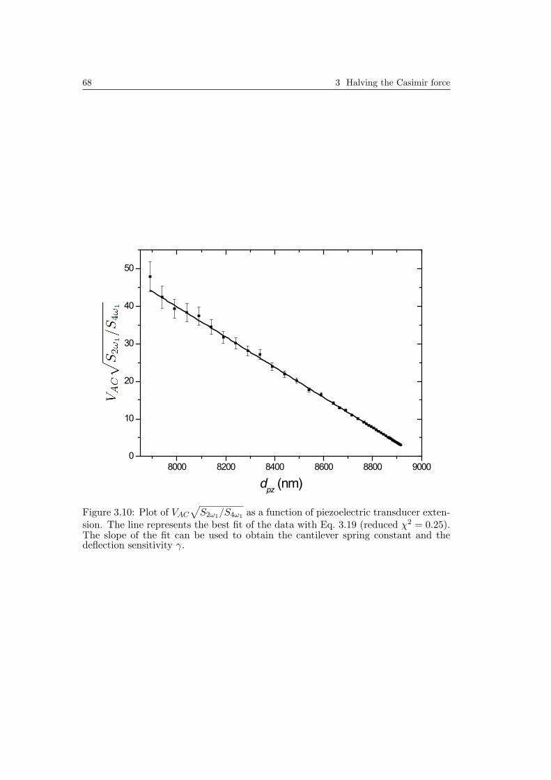
68 3 Halving the Casimir force
8000 8200 8400 8600 8800 90000
10
20
30
40
50
dpz (nm)
Figure 3.10: Plot of VAC√S2ω1/S4ω1 as a function of piezoelectric transducer exten-
sion. The line represents the best fit of the data with Eq. 3.19 (reduced χ2 = 0.25).The slope of the fit can be used to obtain the cantilever spring constant and thedeflection sensitivity γ.

3.3 Halving the Casimir force with conductive oxides: experimental details 69
With the deflection sensitivity calibrated, we can now assess the total can-tilever bending and the precision in the measurements of the cantilever deflec-tion. In the measurement runs presented in Figs. 3.6, 3.7 and 3.8, we usedan S2ω1 set point of 4 mV RMS, which corresponds to a cantilever motion of52 pm RMS. Therefore, the static bending of the cantilever due to the elec-trostatic calibration procedure is 74 pm (see Eqs. 3.3 and 3.5). Anyway, thisstatic bending is constant during the measurement run and it is thus auto-matically taken into account in the estimate of d0. The cantilever oscillationsat ω2 caused by the total force gradient and the hydrodynamic interaction are< 80 pm RMS for these measurement runs, which means that the correspond-ing static bending is < 113 pm. It is thus evident that we can safely neglectthe static bending of the cantilever in our data analysis. Since the noise inS2ω1 is 30 µV RMS, the precision in the detection of the cantilever deflectionis 400 fm RMS with our 1 s RC time (24 dB low-pass filter). This means thatour setup has an RMS sensitivity of 1 pm/
√Hz at 2ω1/2π = 144.4 Hz.
Halving the Casimir force
We now present a comparison between two experiments performed with thesame gold coated 100 µm radius sphere and two different plates. The firstexperiment is conducted with a polished sapphire substrate coated with a goldfilm similar to the one deposited on the sphere. The general performanceof our setup was discussed above by analyzing this first experiment. Thesecond experiment consists of 580 measurement runs in which the plate isreplaced by a float glass substrate with a sputtered ITO thin film on top(PGO CEC010S, typically 8.5 Ω/, or, equivalently, ρ = 1.6 10−4 Ωcm).After purchase, this sample has been exposed to air for more than two yearsbefore our measurements were performed.
Fig. 3.11 shows the Casimir force gradient between the two pairs of sur-faces (Au-Au in green triangles, Au-ITO in red squares) [20]. In Fig. 3.11 a,we plot the force gradients as a function of separation on a double logarithmicscale for randomly chosen subsets of the data (150 out of 580 for both cases).Both datasets are obtained with the exact same settings for the electrostaticcalibration and the force gradient measurement, and the Casimir force gradi-ent is obtained from Eq. 3.11. The black lines indicate the theoretical forcegradient, as will be explained below. Figs. 3.11 b and c present two histogramsof all 580 Casimir force gradient measurements for both Au-Au and Au-ITOat separations d = 120 nm and d = 80 nm, respectively. It is clear that theinteraction strength with the ITO sample is considerably reduced with respectto the gold plate.
Note that our estimate of d0, and thus d, relies on the simple form of Eq. 3.1and is only valid for d R (PFA). This assumption is not entirely correctin the probed separation range [19] and results in a systematic error in d0 of

70 3 Halving the Casimir force
60 80 100 120 140 160 180 2001
10
100
d (nm)
5 10 15 20 25
40 50 60 70 80 90
(a)
~ 40%
~ 50%
(b)
(c)
Figure 3.11: a, Casimir force gradient as a function of separation for the Au-Au(green triangles) and Au-ITO (red squares) interactions for randomly chosen subsetsof the data (150 out of 580 for both cases) plotted on a double logarithmic scale,with the common electrostatic background subtracted from the data. The blacklines correspond to the calculated Casimir interactions. b, Histogram of all 580force measurements for both the Au-Au and Au-ITO measurements at d = 120 nm.The difference in Casimir force gradient is ' 50% between the gold and ITO mea-surements. c, Same as b, but for d = 80 nm. At this separation, the difference inthe force gradient is ' 40%.

3.3 Halving the Casimir force with conductive oxides: experimental details 71
about 1.4 nm. Still, the corresponding underestimate of the separation is equalfor both the measurements with Au and ITO, and can thus be neglected inthe comparison of the two experiments.
Concerning the compensation voltage, we observed that V0 varies approx-imately 1 mV and 3 mV over the complete measurement range in the Au-Auand Au-ITO cases, respectively. These slight variations of V0 do not compro-mise the measurement of the Casimir force at the current level of sensitivity.The value of V0 drifts in time from −106 to −103 mV for Au-Au and from 72to 50 mV for Au-ITO at d = 100 nm. It is also important to note that, duringthe whole duration of the experiment, we never observed any problem withelectrostatic charging of the Au or ITO layers, which would have most likelyresulted in erratic behavior of α and/or V0.
In order to compare the obtained Casimir force gradients with theoreticalpredictions, we have investigated the dielectric properties of our surfaces. InFig. 3.12, we show the reflection and transmission spectra of the two plates,measured from the thin film side, in the frequency range from 0.5 to 6.5 eV.The black continuous lines represent the reflection and transmission spectracalculated from the literature. For Au, we used the values reported in [63].The imaginary part of the dielectric function of ITO is constructed from asum of Drude and Tauc-Lorentz models with the parameters from [64]. Thereal part of the dielectric function is calculated with direct Kramers-Kronigintegration. The thickness of the ITO thin film is fitted by examining theinterference fringes in the reflection and transmission spectra (taking into ac-count the refractive index of the material) and turned out to be 190 nm, whichis close to the typical thickness reported by the manufacturer (180 nm). Theagreement between the spectroscopic measurements and these literature valuesis reasonable in the probed energy range. We want to stress that for Au thereare no adjustable parameters whatsoever in Fig. 3.12, and that for ITO onlythe thickness was fitted. These results allow us to estimate the Casimir forceexpected in the two cases (Au and ITO) and compare the calculation with ourmeasurements (see Eq. 3.12).
The theoretical Casimir interaction is calculated with the Lifshitz equationusing the dielectric properties of our surfaces. For Au, we have extrapolated thedata of [63] with a Drude model (ωp = 9.0 eV and 1/τ = 0.035 eV from [27]).For ITO, we used the model from [64] for all frequencies. The computed forcegradient is plotted as the black lines in Fig. 3.11. The agreement betweendata and theory is reasonable, although we do seem to obtain different powersfor data and theory. At small separation, the experimental curves are bendingupwards, which is a sign of surface roughness effects [67]; the theoretical curveswere calculated for perfectly smooth surfaces. Furthermore, the Au-Au datatend to give rise to a stronger force at large distance compared to theory, whichis most likely caused by an artifact common to many AFM force measurements:the laser light is reflected from the planar sample into the photodetector giving

72 3 Halving the Casimir force
0.00.20.40.60.81.0
1 2 3 4 5 6
0.0
0.5
1.0
1.5
0.00.20.40.6
0.8
1 2 3 4 5 60.00.20.40.6
0.8
R
T x
100
R
T
energy (eV)
Au
Au
ITO
ITO
Figure 3.12: Measured reflection (R) and transmission (T) spectra as a functionof photon energy for the Au on sapphire (green data) and ITO on float glass (reddata) samples. The continuous black lines are calculations of the reflection andtransmission spectra expected for our samples (no fit parameters except ITO layerthickness), using handbook data for gold [63] and a model from [64] for ITO. Thetransmission spectra for gold are zoomed in because the maximum transmission(around 2.5 eV) is only 1.4%. The calculation of the transmission spectrum of theITO sample is quite sensitive to the choice of dielectric properties of the float glass forphoton energies above 4 eV. The black lines describe the measured data reasonablyenough to allow for calculations of the Casimir force.

3.3 Halving the Casimir force with conductive oxides: experimental details 73
rise to a background signal. In the Casimir force gradient method presentedhere, this artifact results, in first order, to an offset in the data; this explainsthe upwards trend of the data for large d. Although the precise distancedependence and strength of this artifact is unknown, we estimate from the forcegradient data at large separation (d > 500 nm) that the associated systematicerror is certainly < 2 N/m2. In the case of the Au-ITO measurements, such abackground signal is a lot smaller because ITO does not reflect well the laserlight (see Fig. 3.12 at ω = 1.9 eV). To explain the mismatch, it is therefore morelikely that the model we used for the dielectric properties [64] is too metallicat low energy and that, consequently, the calculated Casimir interaction is toostrong especially at large d.
(a) (b)
(c)
2.5 5.0 7.5 10 μm 2.5 5.0 7.5 10 μm0 0
63 μm
47 μm -5.15 μm
2.61 μm
0.0
nm
5.0
0.0
nm
20.0
Figure 3.13: a,b AFM topography scans (10 by 10 µm) of the surfaces of the Au onsapphire and ITO on float glass samples, respectively. The surface roughness for thegold sample is 0.8 nm RMS, while the ITO plate has a surface roughness of 4 nmRMS. c, Optical profiler scan of the bottom of the gold coated polystyrene spherethat is attached to the cantilever for our force measurements. The surface roughnessof the sphere is 3.8 nm RMS.
So far, we have neglected the effects of surface roughness in our analysis.In Fig. 3.13, we show topology measurement of our surfaces. Figs. 3.13 a and bare AFM tapping-mode scans (10 by 10 µm) of the Au on polished sapphireand ITO on float glass samples, respectively. The gold sample has an RMSsurface roughness of 0.8 nm, while the ITO coated plate has a roughness of4 nm RMS. Fig. 3.13 c presents a height profile of the surface of the sphere

74 3 Halving the Casimir force
bottom obtained with an optical profiler. Since the cantilever is mounted at a15 degrees angle with respect to the planar sample surface (this is typical inAFM design), the top of this profile does not correspond to the area of closestapproach in a force measurement. However, this height profile does give us theability to estimate the surface roughness of the sphere, resulting in a value of3.8 nm RMS.
Since we used the same sphere in both sets of measurements, the surfaceroughness of the sphere can never cause the observed difference in Casimirforce gradients between the Au-Au and Au-ITO cases. Furthermore, we recallthat surface roughness tends to enhance the strength of the Casimir interac-tion [67]. It is therefore impossible that the different surface roughnesses ofthe two planar samples is responsible for the difference reported in Fig. 3.11,because the ITO sample is considerably rougher than the gold coated sapphiresubstrate.
100 1000
100
200
300
400
500
d (nm)
Figure 3.14: Hydrodynamic force (RMS) acting on the sphere as a function of sep-aration for a subset of the data (150 out of 580 for both cases), caused by theoscillations of the plate surfaces at 119 Hz. The green triangles represent the forcein the case of two gold-coated surfaces, while the red squares correspond to theAu-ITO interaction.
When we discussed the experimental details of our experiment, we men-tioned the interesting feature that we can measure both the Casimir forcegradient and the hydrodynamic force acting on the sphere with the same lock-

3.3 Halving the Casimir force with conductive oxides: experimental details 75
in amplifier at ω2. Fig. 3.14 shows the hydrodynamic force for both the Au-Auinteraction (green triangles) and for the Au-ITO case (red squares). We haveplotted the RMS force resulting from the 2.72 nm RMS oscillation of the plateat ω2/2π = 119 Hz. Both curves appear to change exponent at a separationof around 200 nm. This bending is caused by the slip of the air flow acrossthe surfaces, i. e. the fluid velocity at the gas-solid interface is nonzero. Thisphenomenon is treated in [42] and the expressions derived in there describeour data satisfactorily. Concerning the comparison of the two sets of hydro-dynamic data, it is clear that the hydrodynamic forces are very similar in theAu-Au and Au-ITO experiments. Still, there exists a small difference betweenthe two curves of roughly 2%. This difference cannot be caused by an errorin the determination of the initial separation d0, because both data sets areparallel on the double logarithmic plot. We suppose that the cause may liein the different surface roughnesses of the Au and ITO samples that lead todifferent amounts of fluid slip over the sample surfaces.
It is worthwhile to compare our method for the detection of hydrodynamicforces with recent measurements obtained with AFM’s [68, 69]. In [68], thecantilever with sphere is driven at its free resonance and the amplitude andphase of the cantilever motion are used to extract the hydrodynamic force.In [69], two methods were employed to measure the hydrodynamic interactionbetween a colloid sphere and a plate: measuring the static deflection of the can-tilever during a fast approach of the planar sample and analyzing the thermalnoise of the cantilever while slowly approaching the plate towards the sphere.In both papers, however, the separation between the two interacting surfaceswas determined by bringing the sphere and plate into contact, a method thatis prone to inaccuracies due to surfaces asperities (this is also reported in [69]).Since our method employs both a hydrodynamic force measurement and a pre-cise calibration of the distance at the same time, we have developed a morereliable technique for hydrodynamic force measurements.
3.3.4 Conclusions
We have presented the experimental details of our Casimir force measurementsbetween gold and ITO surfaces [20]. We have shown that the mechanical driftof our setup is less than 0.1 nm per measurement run and that our electrostaticcalibration is performed with 0.2% precision. Force gradient data obtained overapproximately 72 hours reveal no drift in the signal at all, confirming the highstability of the setup. Furthermore, we have introduced and demonstrated anew method to determine the spring constant of our cantilever and the de-flection sensitivity of the AFM readout. We also presented our measurementsof the Casimir and hydrodynamic interactions between the gold and ITO sur-faces, and provided a complete characterization of our samples in terms oftheir dielectric properties and surface roughness.

76 3 Halving the Casimir force
Acknowledgments
The authors thank R. J. Wijngaarden, A. Baldi, F. Mul, and J. H. Rector foruseful discussions. This work was supported by the Netherlands Organisationfor Scientific Research (NWO), under the Innovational Research IncentivesScheme VIDI-680-47-209. DI acknowledges financial support from the Euro-pean Research Council under the European Community’s Seventh FrameworkProgramme (FP7/2007-2013)/ERC grant agreement number 201739.

Chapter 4
Force measurements in gases
4.1 Introduction
In this chapter, we will discuss force measurements at short separation in thepresence of different gases. Concerning the Casimir force, one can understandfrom the Lifshitz equation that the interaction strength, although it dependson the intervening medium between the interacting surfaces, is practically in-sensitive to the choice of gas (contrary to liquids). If one wants to tune theCasimir force with gases, it is thus mandatory to coat the interacting sur-faces with materials whose surface dielectric properties depend on the specificgaseous surrounding. One of such materials are Hydrogen Switchable Mirrors(HSM): reflective metals that upon hydrogen absorption become transparentsemiconductors or insulators. In 2004, Iannuzzi and co-workers at HarvardUniversity performed Casimir force measurements between a gold plate and asphere coated with a HSM in both argon and argon/hydrogen atmosphere. Un-fortunately, they were unable to observe any change in the interaction strengthupon hydrogen exposure. In Section 4.2 we perform a precise computation ofthe Casimir force between gold and HSM surfaces in both the hydrogen loadedand unloaded states, and show that the presence of a Pd capping layer cov-ering the HSM dramatically reduces the difference in Casimir force for bothstates. In fact, this reduction is so strong, that the force contrast betweenboth configurations is smaller than the resolution of the setup that was usedin 2004, which clearly explains the negative result of the experiment.
The setup we describe in this thesis, however, is much more capable ofCasimir force measurements in terms of stability and precision. We havetherefore initiated a second round of Casimir force measurements with HSMs.In section 4.3, we present our force data between a Y/Pd HSM and a goldcoated sphere. Interestingly, we were also unable to observe a decrease in theforce upon hydrogen loading of the HSM, but found, on the contrary, a muchstronger attractive interaction between the two surfaces in H2 atmosphere.This strong interaction has most likely an electrostatic origin, and we will de-fend this claim by examining the distance dependence of the extra force and
77

78 4 Force measurements in gases
of the contact potential.The hydrodynamic interaction between the sphere and the plate depends,
of course, also on which type of gas is present in the gap. In section 4.4, wepresent measurements of the hydrodynamic damping force in air, Ar, He, andSF6. These gases span a wide range of mean free paths, by which we caneffectively explore gas surface slip. In fact, although in He both the gas sliplength and the mean free path are larger than the smallest gap size, it turnsout that the continuous medium theory developed in 1973 by Hocking worksflawlessly at these small separations.

4.2 On the use of Hydrogen Switchable Mirrors in Casimir force experiments 79
4.2 On the use of Hydrogen Switchable Mir-rors in Casimir force experiments
Abstract – Hydrogen Switchable Mirrors (HSMs) are shiny metals that be-come optically transparent upon exposure to hydrogen. The Casimir forcebetween HSMs is thus supposed to be stronger in air than in hydrogen. A fewyears ago, an experiment designed to measure this effect gave an unexpectedresult (Iannuzzi D, Lisanti M and Capasso F 2004 Proc. Nat. Ac. Sci. USA101 4019–23): no change of the force was observed upon hydrogenation. Qual-itative arguments show that this result is reasonable if HSMs do not switch atlong wavelengths, where no measurements of the dielectric function are avail-able. Because the exact composition of the mirrors used in that experimentis not known, a more quantitative comparison of the data with theory is notpossible. Still, calculations of the Casimir force in the presence of similarHSMs of known composition might provide new insights for the interpretationof the experimental result and may suggest precious hints for the developmentof future analogous experiments. In this paper, we present calculations of theCasimir attraction between Mg2Ni mirrors in air and in hydrogen. Our resultsclearly indicate that the modulation of the Casimir force with HSMs shouldbe observable with modern set-ups.
This paper has been published: S. de Man and D. Iannuzzi, New J. Phys. 8, 235 (2006)

80 4 Force measurements in gases
4.2.1 Introduction
In the last decade, the literature dedicated to the Casimir effect [18] has beenstrongly influenced by a series of papers claiming the achievement of ulti-mate accuracy in the comparison of Casimir force experiments with theoret-ical predictions (see for example [70] and references therein). These papershave triggered a renewed interest in this field, stimulating a vivid discussionon the calculation of systematic errors of both experimental data and theoret-ical analysis. It is therefore not surprising that the large majority of modernexperiments are performed using surfaces coated with thick, bulk-like metal-lic layers. From an experimental point of view, the use of metals offers thepossibility to control and eliminate any residual electrostatic interaction thatmight disturb the measurements and increase the experimental uncertainty.Concerning the theoretical analysis of the data, the Casimir force between twoobjects is typically calculated by substituting the dielectric functions of theirsurfaces directly into the Lifshitz equation for van der Waals interaction [23].The accuracy of the predicted results is thus strictly related to the degreeof confidence with which those functions are known. The choice of bulk-likemetallic films facilitates accurate calculations, because the dielectric functionsof metals are known better than those of dielectrics. Measurements of Casimirforces between materials other than metals would thus not contribute to thediscussion on the accuracy issue, giving rise to less impactful results.
It has been already recognized, however, that this trend represents a severenarrowing of the focus of modern literature [7, 32, 33, 71, 72]. The dependenceof the Casimir force on the dielectric function of the interacting surfaces shouldnot be considered only as an annoying detail that makes measurements andprecise calculations more difficult. It should rather stimulate new experimentsthat explore the possibility of tailoring the Casimir effect using materials withsuitably chosen dielectric functions.
(a) (b)
Figure 4.1: An image of a Hydrogen Switchable Mirror (a) before and (b) afterexposure to hydrogen (courtesy of Ronald Griessen).
A few years ago, in the attempt to emphasize the importance of studies

4.2 On the use of Hydrogen Switchable Mirrors in Casimir force experiments 81
that go beyond the accuracy issue, one of us (DI), in collaboration with M.Lisanti and F. Capasso, performed the first measurement of the Casimir forcebetween Hydrogen Switchable Mirrors (HSMs) [32]. HSMs are materials thatalter their dielectric properties upon hydrogen absorption [44] (see Fig. 4.1).They change from reflective conductors to transparent semiconductors or insu-lators when they are transferred from air to hydrogen. The effect is reversible;when the mirror is put back in air, it switches again to the reflective state.Because of this change of their optical properties upon hydrogen absorptionand desorption, HSMs offer in principle the possibility to observe a reversible,in-situ change of the Casimir force between surfaces at fixed separation, a fas-cinating prospect from both a fundamental and technological point of view.According to the Lifshitz theory, the attraction between highly reflective metalsis larger than the attraction between transparent dielectrics, which provide aless efficient confinement of the electromagnetic modes in the cavity formed bythe two interacting surfaces. It should thus be possible to reduce the Casimirforce between HSMs by exposing the mirrors to a hydrogen atmosphere; theforce could then be brought back to higher values by replacing hydrogen withair. Surprisingly, the experiment reported in reference [32] was not capable ofdetecting any effect. In spite of the dramatic change of the optical propertiesof the mirrors, the Casimir force measured in hydrogen was not significantlydifferent from that obtained in air. Due to the limited amount of informationon the dielectric function of the HSMs used in the experiment, the authorscould not present a rigorous theoretical calculation to compare with the data.Nevertheless, a mathematical exercise based on ad hoc materials with properlychosen dielectric functions made it possible to explain this unexpected resultin terms of a counterintuitive property of the Lifshitz theory. Yet, a completeanalysis of the magnitude of the effect is still missing, and one might wonder ifthere is a configuration for which a reversible change of the Casimir force be-tween HSMs upon hydrogenation could be observed with modern experimentalset-ups.
The goal of the present paper is to address this topic. First, we will brieflyreview the previous experiment and the mathematical arguments reported toexplain the data. Then, we will discuss the switching properties of Mg2Nimirrors, HSMs with composition similar to the one used in the experiment. Wewill show that, although direct measurements of reflectivity and transmittivityare available only in a limited wavelength region, it is still possible to estimatethe behavior of the dielectric function over a much broader spectrum by meansof a simultaneous analysis of Hall effect and resistivity data. Finally, we willpresent the results of Casimir force calculation obtained by substituting thesedielectric functions in the Lifshitz equation. We will demonstrate that thedecrease of the attraction after hydrogenation of the mirrors is expected to besmaller than the sensitivity of the experiment discussed above, but sufficientto be observed with an updated version of that apparatus or with one of the

82 4 Force measurements in gases
set-ups that, according to literature, can provide measurements of the Casimirforce with 1% (or better) precision.
4.2.2 Casimir effect with Hydrogen Switchable Mirrors:previous experimental results
Measurements of the Casimir force using HSMs were reported in reference [32](see also [71, 73]).
Figure 4.2: Schematic view of the experimental set-up that has been used for themeasurement of the Casimir force between a gold coated plate and a sphere coatedwith a Hydrogen Switchable Mirror (not to scale) [32]. The four top panels illustratethe rotation of the micromachined see-saw in response of the Casimir interaction withthe sphere.
The set-up used for the experiment is similar to the one originally developedat Bell Laboratories by H. B. Chan, F. Capasso, and their collaborators [2, 3](see Fig. 4.2). The force sensor consists of a micromachined device thatresembles a miniaturized see-saw. A polysilicon plate (0.5 × 0.5 mm2 area),covered with a 5 nm thick chromium adhesion layer and a 200 nm thick goldcoating film, is kept in suspension by means of two thin rods that departfrom the middle point of two opposite sides of the plate and end onto a postanchored to the substrate. The two rods define the pivot axis of the see-saw.Two electrodes, located underneath the plate in a symmetric configurationwith respect to the pivot axis, allow capacitive measurements of the rotation

4.2 On the use of Hydrogen Switchable Mirrors in Casimir force experiments 83
of the top plate with accuracy on the order of 10−7 rad, which corresponds toa torque sensitivity of ' 10−15 Nm.
The force sensor is mounted on top of a calibrated piezoelectric stage andaligned to a polystyrene sphere (100 µm radius) in the position illustrated inFig. 4.2. The separation between the sphere and the top plate of the see-saw can be varied by changing the voltage applied to the piezoelectric stage.For separations d smaller than ' 400 nm, the Casimir attraction between thesphere and the plate is sufficient to induce rotations of the see-saw that arelarger than the experimental sensitivity. With this set-up, it is thus possibleto carry out measurements of the Casimir force between the sphere and theplate from d ' 400 nm down to the jump-to-contact point, i.e., to that valueof d where the restoring force of the torsional rods is not sufficient to overcomethe attractive force between the two surfaces.
In this experiment, spheres were coated with a Pd-capped Mg-Ni HSM [74].The mirror was fabricated by means of seven consecutive depositions of Mg-Nilayers, followed by a single deposition of a 5 nm thick palladium cap. EachMg-Ni layer was obtained by evaporating a 2 nm thick nickel film on top of a10 nm thick magnesium film. The palladium cap was added to promote hydro-gen absorption [44], because, in the conditions of the Casimir force experiment(room temperature and less than atmospheric partial pressure of hydrogen)an uncapped HSM would have not spontaneously absorbed hydrogen. Thepresence of a metallic layer at the interface with the external environment hadanother important function, in that it allowed for the control of electrostaticinteractions. In similar uncapped HSMs, the HSM-to-air interface quickly oxi-dizes. Accumulation of surface charges on the oxide film would have given riseto electrostatic forces that could have easily overcome the Casimir attraction.The deposition of the palladium cap on top of the HSM prevented this processto occur. Furthermore, the presence of a metallic interface, opportunely con-nected to a power supply, gave the possibility to control the potential differencebetween the two interacting surfaces, an essential element in all Casimir forceexperiments [25, 70].
Measurements of the Casimir force FC between a HSM-coated sphere andthe top plate of the see-saw were carried out as a function of separation dfollowing the scheme described in reference [32]. We refer the reader to theoriginal paper for a detailed explanation of the data acquisition technique.Here we only want to stress that this technique allows one to calibrate theset-up with electrostatic forces and to perform, simultaneously, FC-versus-dmeasurements.
Measurements were carried out in air and in a 4% hydrogen-in-argon mix-ture at room temperature and nearly atmospheric pressure, and repeated usingdifferent spheres and force sensors. A comparison of the data obtained beforeand after hydrogen loading reveals that there was no significant change in theCasimir force upon hydrogenation of the HSM [32].

84 4 Force measurements in gases
4.2.3 Casimir effect with Hydrogen Switchable Mirrors:qualitative analysis of the experimental results
The results reviewed above have been qualitatively explained in reference [32].The dielectric function of Mg-Ni HSMs is known only in a wavelength re-gion that approximately spans from 0.2 µm to 2.5 µm [74], where reflectivityswitches from ' 70% to ' 20% upon hydrogenation. Very little informationis available at longer wavelengths, where HSMs might not switch at all. Itis thus important to understand whether those longer wavelengths contributeto the Casimir force between surfaces at sub-micron separation. If infraredmodes are relevant and HSMs do not switch in the infrared spectrum, thedecrease of the Casimir force might be too small to be observable with theexperimental set-up described in the previous section. The following mathe-matical exercise demonstrates that infrared modes do play a significant rolein the Casimir interaction at those distances, and that the change in the forceupon hydrogenation is dramatically hampered if one assumes that these HSMsdo not switch at long wavelengths.
The Casimir force between a plate made out of a material 1 and a spheremade out of a material 2 separated by a medium 3 can be calculated by plug-ging the dielectric functions of the interacting surfaces and of the interveningmedium directly into the Lifshitz equation for van der Waals interaction [23]:
FC(d) =~R
2πc2
∫ ∞0
∫ ∞1
ε3pξ2
log[1−∆
(1)31 ∆
(1)32 e−x]+log
[1−∆
(2)31 ∆
(2)32 e−x]
dp dξ
(4.1)where ~ is the reduced Planck’s constant, R is the radius of the sphere∗, c isthe speed of light in vacuum,
∆(1)jk =
skεj − sjεkskεj + sjεk
∆(2)jk =
sk − sjsk + sj
(4.2)
and
x =2d√ε3ξp
csj =
√p2 − 1 +
εjε3
(4.3)
In Eqs. 4.1, 4.2 and 4.3, εj stands for the dielectric function evaluated atimaginary frequency, εj(iξ). This quantity is defined by the following relation:
εj (iξ) = 1 +2
π
∫ ∞0
ωε′′j (ω)
ω2 + ξ2dω (4.4)
where ε′′j (ω) is the imaginary part of the dielectric function.
∗Note that Eq. 4.1 relies on the Proximity Force Approximation, which is acceptable onlyif R d

4.2 On the use of Hydrogen Switchable Mirrors in Casimir force experiments 85
In the experiment described in the previous section, the intervening mediumwas either air or a hydrogen enriched gaseous mixture kept at room tempera-ture and nearly atmospheric pressure. One can thus assume ε3(iξ) = 1 at allfrequencies.
Following references [32, 71], we can now define an ad hoc material whosedielectric function (at real frequencies) is identical to that of gold, with theexception of a wavelength range that spans from λmin to λmax, where ε′′ isassumed to be identical to zero. Using Eq. 4.1, we can then calculate theCasimir force between a sphere and a plate made out of this hypotheticalmaterial. If we assume that infrared modes do not contribute to the Casimirinteraction, the values of ε′′ at wavelengths larger than ' 1 µm should notbe of any relevance. The Casimir force expected for an ad hoc material withλmin = 1 µm and λmax = 200 µm should thus not differ from the attractionbetween two gold surfaces.
Calculations reveal that, on the contrary, the value of ε′′ at long wavelengthsis of great importance for a correct evaluation of the Casimir force at sub-micron separations. For d = 100 nm, for example, the Casimir attractionbetween a sphere and a plate made out of an ad hoc material with λmin = 0.3µm and λmax = 2.5 µm is only ' 3% smaller than that expected between goldsurfaces. However, if one assumes λmin = 1 µm and λmax = 200 µm, thisdifference becomes significantly higher, reaching ' 35%.
This behavior is due to the fact that the Lifshitz equation (Eq. 4.1) isintimately connected to the dielectric function of the interacting materialscalculated at imaginary frequencies, which can be obtained by means of Eq.4.4. For every imaginary frequency iξ, the imaginary part of the complexdielectric function ε′′ is integrated over all real frequencies, with non-negligiblecontributions arising from a wide range of modes.
In the original paper [32], it was stressed that the theoretical discussion wasnot accounting for the presence of the thin palladium layer that was added ontop of the HSM. The thickness of this coating film is smaller than the skin-depth and should intuitively not contribute significantly to the interaction.However, the authors suggested that a more rigorous calculation might revealthat this thin metallic layer plays a counterintuitive role. We will come backto this point in the next section.
4.2.4 Casimir effect with Hydrogen Switchable Mirrors:is the modulation of the force observable?
While the arguments reported above provide a reasonable qualitative explana-tion of the experimental results, it would be interesting to perform a rigorouscomparison of the data with theory. Unfortunately, this is not feasible. It isknown that the dielectric function of Mg-Ni HSMs strongly depends on theircomposition and on their hydrogen content upon hydrogenation [74]. Due to

86 4 Force measurements in gases
the fabrication technique used in the experiment (consecutive deposition ofthin layers of magnesium and nickel), it is not possible to establish the ex-act composition (neither before nor after hydrogenation) of those particularfilms, which might even have been non-homogeneous. Any attempt to providea more quantitative comparison of the data with theory would inevitably bebased on very rough approximations on the composition of the mirrors. Theseapproximations would lead to ambiguous conclusions.
It is possible, however, to calculate the magnitude of the decrease of theCasimir force between similar HSMs of known composition. The results mightprovide a clear indication on the feasibility of an experimental observation ofthe effect, and might also emphasize potential problems that were not consid-ered in the previous experiment.
To achieve this goal, we have calculated the Casimir attraction between agold plate and a 100 µm radius sphere coated with a palladium capped Mg2Nimirror. The first step to perform the calculation is to evaluate the dielectricfunction of the HSM both in its reflective and in its transparent states (i.e., inair and in hydrogen, respectively).
It is known that, in the optical frequency range, HSMs can be well describedby a Drude-Lorentz model [75]:
ε (ω) = ε∞ −ω2p
ω2 + iωτ
+∑j
fjω2
0j − ω2 − iβjω (4.5)
The model includes a Drude contribution arising from the presence of freecharge carriers with plasma frequency ωp and relaxation time τ , and a series ofLorentz oscillators with strengths fj, resonance frequencies ω0j and dampingterms βj. Because Eq. 4.5 is analytic, the dielectric function at imaginaryfrequency can be simply obtained by substituting ω with iξ:
ε(iξ) = ε∞ +ω2p
ξ2 + ξτ
+∑j
fjω2
0j + ξ2 + βjξ(4.6)
The Drude-Lorentz parameters ωp, τ , fj, ω0j, βj, and ε∞ for Mg2Ni HSMswere obtained by Lohstroh et al., who analyzed reflectivity and transmittiv-ity measurements in the wavelength region spanning from ultraviolet to nearinfrared [76, 77]. According to their results, for mirrors in the reflective state(i.e., mirrors in air before exposure to hydrogen), one Lorentz oscillator andone Drude term are sufficient to reproduce the experimental data. For mirrorsin the fully loaded transparent state (i.e., after complete hydrogenation, cor-responding to Mg2NiH4−δ, with δ ' 0), four Lorentz oscillators are necessary,but no Drude tail is needed†. Optical data, in fact, do not reveal any Drude-like
†We thank the authors for providing us with the values of the Lorentz parameters: ε∞ =2.45,
√f1 = 2.67 eV, ω01 = 2.54 eV, β1 = 0.40 eV,
√f2 = 3.62 eV, ω02 = 3.08 eV,
β2 = 0.69 eV,√f3 = 4.32 eV, ω03 = 3.87 eV, β3 = 1.40 eV,
√f4 = 4.48 eV, ω04 = 5.64 eV,

4.2 On the use of Hydrogen Switchable Mirrors in Casimir force experiments 87
1 10 1000.0
0.2
0.4
0.6
0.8
1.0
R
( m)
1
2
3
4
Figure 4.3: Reflectivity of Mg2Ni Hydrogen Switchable Mirrors as a function ofwavelength. The shaded area represents the wavelength region were experimentaldata are available. Curve 1 refers to a Drude-Lorentz model that fits the opticaldata of the mirror in its reflective state (before switching). Curve 2, 3, and 4 referto hydrogenated Hydrogen Switchable Mirrors. Curve 2 represents a Lorentz modelobtained by fitting the optical data. Curve 3 is equivalent to Curve 2, with theaddition of a Drude term obtained from the combined analysis of Hall effect andresistivity measurements. Curve 4 is the sum of curve 2 and a Drude term with adhoc plasma frequency and relaxation time.

88 4 Force measurements in gases
1 10 1000
5
10
15
201
"
( m)
4 3
2
Figure 4.4: Imaginary dielectric function of Mg2Ni Hydrogen Switchable Mirrors asa function of wavelength. Symbols are equivalent to those used in Fig. 4.3.

4.2 On the use of Hydrogen Switchable Mirrors in Casimir force experiments 89
behavior up to the longer wavelengths investigated (' 2.5 µm). To understandthe relevance of this point, in Fig. 4.3 and Fig. 4.4 we plot, respectively, thereflectivity and the dielectric function of Mg2Ni HSMs before and after switch-ing. The shaded area represents the wavelength region where experimentaldata are available. Curve 1 refers to the fitting function proposed by Lohstrohet al. for Mg2Ni HSMs before hydrogenation. Curve 2 corresponds to thefitting function proposed by the same group for the hydrogenated state, withfour Lorentz oscillators and no Drude term. Curves 3 and 4 were obtained byus using the same function as in curve 2 with an additional Drude tail‡. Theprecise meaning of these curves will be clarified later in the text. Here we wantto stress that curves 2 and 3, which have different behavior in the infrared,are very similar over the whole wavelength region where experimental data areavailable. None of these curves is thus in contradiction with the experiment. Itis then evident that a correct extrapolation of the dielectric function at longerwavelengths cannot rely on these data. Unfortunately, these data still repre-sent the only direct source of information available: to our knowledge, in fact,optical properties of HSMs have never been systematically measured beyond' 2.5 µm§.
In the absence of more direct experiments, it is still possible to estimatethe Drude term in fully hydrogenated Mg2Ni HSMs by a combined analysisof Hall effect and resistivity measurements. Hall effect experiments provide adirect measurement of the density of free charge carriers n [79]. If resistivity isknown, one can then calculate the dissipation factor and the plasma frequencyof the Drude term using the following equations [79]:
τ =
(0.22
ρµ
)(rsa0
)3
× 10−14 sec (4.7)
ωp = 7.27
(a0
rs
)3/2
× 1016 rad sec−1 (4.8)
where ρµ is the resistivity in µΩcm, a0 is the Bohr radius, and rs is given by
rs =
(3
4πn
)1/3
(4.9)
Magnetoresistance and charge carrier density of Mg2Ni HSMs were measuredby Enache et al. for different hydrogen concentrations [80]. For fully loaded
β4 = 3.03 eV.‡For curve 4, the oscillator strengths of the Drude-Lorentz model fj were multiplied by
a factor of 0.9.§In reference [78], the authors reported measurements of the reflection and transmission
coefficients up to 6 µm. However, raw data were not analyzed in terms of the Drude-Lorentzmodel, and cannot be used in our calculations. It is however important to emphasize thatthose measurements do not reveal any Drude tail in the wavelength region between 2.5 µmand 6 µm, still in agreement with curves 2 and 3.

90 4 Force measurements in gases
mirrors, the authors obtained n = 9.28 ·1020 carriers/cm3 and ρ = 12.9 mΩcm.
We can now comment further on Fig. 4.3 and Fig. 4.4. We recall that curve1 represents the HSM in its high reflectivity state¶, and that curve 2 was ob-tained by fitting the optical data from visible to near infrared with four Lorentzoscillators and no Drude term. This model, which is equivalent to assume thatHSMs become highly transparent at long wavelengths, is not consistent withHall effect and resistivity measurements, and must thus be considered incorrectin the infrared spectrum. Curve 3 is equivalent to curve 2 plus a Drude termcalculated according to the arguments reported above; it represents the bestestimation of reflectivity and dielectric function of Mg2NiH4−δ (with δ ' 0)that one can obtain with the data available in literature. Curve 4 is again anad hoc model that will serve to stress once more the importance of infraredmodes in the Casimir interaction. The properties of this hypothetical mirrorare in contradiction with Hall effect and resistivity measurements.
At this point, we have enough information to model the Mg2Ni mirrorsin air (model 1) and in hydrogen (model 3), and to discuss the consequencesthat the use of erroneous models for the hydrogenated state would have inthe calculation of the Casimir force upon hydrogenation (models 2 and 4).The presence of a thin palladium layer deposited on top of the mirror can beintroduced in the calculation by means of a model developed by Parsegian andNinham [81], according to which the Casimir force between a material 2 anda material 1 covered with a cap layer 4 of thickness t4, immersed in a medium3, is obtained from Eq. 4.1, replacing ∆
(1,2)31 with
∆(1,2)31 → ∆
(1,2)34 + ∆
(1,2)41 e−
xt4s4pd
1 + ∆(1,2)34 ∆
(1,2)41 e−
xt4s4pd
(4.10)
In order to run the calculation, it is still necessary to evaluate the dielectricfunction of the gold plate and of the palladium layer. For these materials, weuse the tabulated data for the corresponding bulk metal [63] plus a Drude termas described in reference [27] (for gold) and reference [82] (for palladium).
In Fig. 4.5 we report the results of the calculations. The graphs show thedecrease of the Casimir force between a gold plate and a 100 µm sphere coatedwith a Mg2Ni HSM, alternatively exposed to either air or hydrogen. FR andFT indicate the force for the reflective state and for the optically transparenthydrogenated state, respectively. d is the separation between the sphere andthe plate. Different curves refer to different models of the hydrogenated state(see table 4.1), and have been numbered in accordance with Figs. 4.3 and4.4. Curves 2, 3, and 4 were obtained neglecting the presence of the palladiumfilm. Concerning curve 3-Pd, a 5 nm thick palladium layer was added to the
¶It is interesting to note that, for the reflective state (Mg2Ni), the combined analysisof Hall effect and resistivity measurements gives rise to plasma frequency and dissipationfactor values that are in agreement with those obtained from optical data [76].

4.2 On the use of Hydrogen Switchable Mirrors in Casimir force experiments 91
Mate
rial
Desc
ripti
on
HSM
reflec
tive
stat
e1
Lor
entz
Osc
illa
tor
(Ref
.[7
6])
plu
sM
odel
1D
rude
term
:ωp
=1.
24·1
016
rad/s
;τ
=9.
9·1
0−16
sH
SM
hydro
genat
edst
ate
4L
oren
tzO
scilla
tors
(Ref
.[7
7])
Model
2N
oD
rude
term
HSM
hydro
genat
edst
ate
4L
oren
tzO
scilla
tors
(Ref
.[7
7])
plu
sM
odel
3D
rude
term
:ωp
=0.
17·1
016
rad/s
;τ
=2.
96·1
0−16
sH
SM
hydro
genat
edst
ate
4L
oren
tzO
scilla
tors
(Ref
.[7
7])∗
plu
sM
odel
4D
rude
term
:ωp
=1.
43·1
016
rad/s
;τ
=1.
82·1
0−17
sG
old
surf
ace
Tab
ula
ted
dat
a(R
ef.
[63]
)plu
sD
rude
term
:ωp
=1.
37·1
016
rad/s
;τ
=1.
88·1
0−14
s(R
ef.
[27]
)P
alla
diu
mla
yer
Tab
ula
ted
dat
a(R
ef.
[63]
)plu
sD
rude
term
:ωp
=0.
83·1
016
rad/s
;τ
=4.
28·1
0−14
s(R
ef.
[82]
)
Tab
le4.
1:Su
mm
ary
ofth
em
odel
sus
edfo
rth
eca
lcul
atio
nsre
port
edin
the
text
.T
heas
teri
skad
ded
inth
ede
scri
ptio
nof
mod
el4
indi
cate
sth
at,
for
this
part
icul
arm
odel
,th
eos
cilla
tor
stre
ngth
sof
the
Lor
entz
term
have
been
mul
tipl
ied
bya
fact
or0.
9.

92 4 Force measurements in gases
50 100 150 200 250 300 350 400-50
-40
-30
-20
-10
0
(FT
- FR)
/ F R
(%
)
d (nm)
2
3
4
3-Pd
100 300
100
300
F (p
N)
d (nm)
1-Pd
3-Pd
Figure 4.5: Expected decrease in the Casimir force between a gold plate and a100 µm radius sphere coated with a Hydrogen Switchable Mirror exposed to eitherair or hydrogen. FR and FT indicate the force for the reflective state and for thetransparent hydrogenated state, respectively. d is the separation between the sphereand the plate. Calculations were performed using the dielectric functions reportedin Fig. 4.4 (see also table 4.1). Different curves refer to different models of thehydrogenated state, and have been numbered in accordance with Figs. 4.3 and 4.4.The suffix ′′Pd′′ indicates whether the 5 nm thick palladium coating layer was takeninto account in the calculations or not. Inset: comparison of the results of thecalculations with the experimental data reported in reference [32]. Light and darkgray symbols refer to measurements performed in air and hydrogen, respectively.

4.2 On the use of Hydrogen Switchable Mirrors in Casimir force experiments 93
calculation of both FT and FR. From this graph, two important conclusionscan be drawn.
• Curves obtained with no Drude term (curve 2), with the correct Drudeterm (curve 3), and with the fictitious Drude term (curve 4) are signif-icantly different. This result emphasizes once more that if one assumesthat hydrogenated HSMs remain highly reflective at long wavelengths,the decrease of the force upon hydrogenation is much smaller than thatexpected with a wide band switching mirror. Long wavelengths are thusindeed relevant, as already pointed out in reference [32].
• The 5 nm thick palladium capping layer deposited on top of the HSMplays a dramatic role in the interaction. At 100 nm separation, thechange of the Casimir force upon hydrogenation for an uncapped mirroris larger than 35% (curve 3); if the palladium layer is added (curve 3-Pd), the effect reduces to ' 20%. Further calculations show that a 10nm thick palladium would decrease the change of the force at 100 nmto ' 10%. The palladium layer represents a serious obstacle for theobservation of large Casimir force modulations.
In the inset of Fig. 4.5 we report a direct comparison of the calculationswith the experimental data of reference [32]. We want to stress once more thatthe curves represent the results of calculations performed using the propertiesof materials that probably have a different composition with respect to the onesused in the experiment. Nevertheless, the graph allows us to emphasize that,even in the best case scenario of fully loaded HSMs with fairly good switchingproperties in the infrared, the effect could have been hardly observed with theexperimental sensitivity of the set-up described in [32].
It is to note that our calculation relies on the hypothesis that the HSMin use undergoes full hydrogen loading upon hydrogenation. Partial loadingwould significantly alter the result. It is known, in fact, that the loading processin Mg2Ni HSMs (and, more generally, in most of Mg-Ni compounds) involves aremarkable self-organized double layering [83]. Hydrogen first penetrates insidethe film and quickly reaches the substrate, from where hydrogenation starts(see inset of Fig. 4.6). Partial loading leads to a bi-layered structure formedby a transparent layer close to the substrate and a non-switched metallic layerclose to the palladium film. This non-switched metallic layer is still highlyreflective. Its presence would have a dramatic effect on the Casimir force, asit increases the overall thickness of the metallic film above the hydrogenatedpart of the mirror (see Fig. 4.6). Note that it is not possible to establishwhether the HSMs used in the experiment of reference [32] were fully loaded.The presence of a non-switched layer below the palladium film might havecontributed to reduce the magnitude of the Casimir force difference betweenmeasurements in air and in hydrogen.

94 4 Force measurements in gases
(a)
(b)
PdReflective part of the mirrorTransparent part of the mirrorSubstrate
(c)
In air
Partialloading
Fullloading
hydrogenation
hydrogenation
Figure 4.6: Schematic view showing that partial loading of Hydrogen SwitchableMirrors plays a detrimental role in Casimir force modulation experiments. Sketch (a)refers to the mirror before hydrogenation; sketch (b) shows the layered structure thatwould form in case of partial hydrogen loading, with a relatively thick reflective layerstill present at the interface; sketch (c) illustrates the absence of layered structuresat the interface in fully loaded mirrors. Inset: schematic diagram of the hydrogenloading mechanism in Mg-Ni Hydrogen Switchable Mirrors.
4.2 On the use of Hydrogen Switchable Mirrors in Casimir force experiments 95
Our analysis also neglects the correction to the Casimir force due to thesurface roughness of the interacting objects. These corrections cannot be ex-plicitly calculated a priori, because the morphology of HSMs strongly dependson the deposition technique [84]. In this respect, it is worth stressing that thesurface profile of HSMs in air undergoes large variations during the first fewhydrogen loading and unloading cycles [84, 85], after which no more morpho-logical adjustments are observed. Therefore, reproducible modulations of theCasimir force with HSMs can be achieved only after the mirrors have beenswitched a few times. It is also evident that for a correct interpretation ofthe data, accurate measurements of the morphology of the surfaces both inair and in hydrogen are needed, because the alteration of the roughness uponhydrogenation could mimic or hinder the decrease of the Casimir force inducedby the change of the optical properties of the mirrors.
4.2.5 Conclusions
Tuning the Casimir force with HSMs is a fascinating opportunity that callsfor deeper investigations. The only measurements reported so far [32] wereaffected by a relatively large experimental error, which was mainly due tothe fact that the experiment was carried out at atmospheric pressure. Thechange in the force upon hydrogenation was smaller than intuitively expected,and was not sufficient to be observed. A qualitative theoretical analysis firstshowed that the results could have been explained assuming that the dielectricfunction of HSMs switches only in a limited wavelength region that spansfrom ultraviolet to near infrared, where optical data are available [32]. Longerwavelengths play in fact an important role in the interaction: if the mirrorremains highly reflective in the infrared part of the spectrum, the change inthe force upon hydrogenation can be smaller than the experimental sensitivity.A more complete theoretical analysis of the experiment was not performed,because the exact composition of the mirrors was not known.
In this paper we have calculated the expected decrease of the force forsimilar mirrors of known composition (Mg2Ni). The results confirm the mainconclusion of reference [32]: for an accurate comparison of experimental datawith theory it is necessary to know the value of the dielectric functions of theinteracting materials over a broad wavelength range that extends up to thefar infrared region. Furthermore, the presence of a palladium capping layerstrongly reduces the effect. Still, at 100 nm separation, the Casimir force isexpected to decrease ' 20% upon full hydrogenation. We thus believe that itis possible to design a new experiment for the first observation of an in situmodulation of the Casimir force between HSMs. A significant reduction of theexperimental uncertainty can be obtained by performing the measurementsin vacuum. It is known that, in vacuum, hydrogenated HSMs do not releasehydrogen. One could thus load or unload the mirror by flushing the measuring

96 4 Force measurements in gases
chamber with proper gases at atmospheric pressure (hydrogen for loading, andair for unloading), and then pump vacuum during Casimir force measurements.In order to obtain a more pronounced effect, it would be also desirable to reducethe contribution of the thin palladium layer deposited on top of the HSM. Theuse of films thinner than 5 nm is in principle a possible solution to this problem.However, the resulting layer would probably be discontinuous after switching[85] and would not allow a complete control of electrostatic forces. A possiblealternative is to replace palladium with a metal that wets the mirror betterthan palladium does, and then use hydrogen diffusion from a palladium padlocated away from the interaction region (i.e., away from the portion of thesphere that, upon assembling of the experimental set-up, stands in front ofthe force sensor) to obtain uniform switching [86, 87]. This choice might allowone to reduce the thickness of the cap layer down to 2 or 3 nm. A moreprecise experiment would also probably stimulate a more accurate comparisonwith theory. Direct measurements of the dielectric functions in the infraredwavelength region and of the surface morphology of the films deposited ontothe interacting surfaces would certainly facilitate a rigorous interpretation ofthe experimental data.
Acknowledgements
We are particularly indebted with J. N. Munday for his initial contributionto this work, and to R. Griessen for his critical analysis of the manuscript.We thank D. Borsa, C. Broedersz, F. Capasso, B. Dam, W. Lohstroh andR. Westerwaal for useful discussions, and the Netherlands Organisation forScientific Research (NWO) for financial support, which was granted throughthe Innovational Research Incentives Scheme Vernieuwingsimpuls VIDI-680-47-209.

4.3 Force measurements in H2 gas 97
4.3 Force measurements in H2 gas
Abstract – We present force measurements between a gold coated sphere anda planar sample coated with a Y/Pd hydrogen switchable mirror. Measure-ments were performed in air, argon and argon/hydrogen mixture. First, weprove that our setup is capable of working in hydrogen atmosphere by ana-lyzing our measurements of the hydrodynamic force. Then we show that inhydrogen atmosphere, the force gradient detected between the sphere and theplate is much stronger than expected. A comparison of these data with datain pure argon suggests that this extra force gradient component has an electro-static origin, since it follows a power law with relatively small exponent -2.35.Third, we present the simultaneously acquired contact potential measurementsand show that although V0 is rather constant as a function of separation in ar-gon, it strongly depends on the distance in the argon/hydrogen mixture. Thisobservation further enhances our suspicion that the stronger force gradientmeasured in hydrogen atmosphere has an electrostatic origin.

98 4 Force measurements in gases
In the previous section, we have calculated the force between a Mg/Niswitchable mirror and a gold sphere in both the hydrogen loaded and unloadedstates of the mirror. We concluded that the change in force upon hydrogenationof the HSM should be around 20%. With the current experimental setup, sucha change should be easily observable. Therefore, we have upgraded our systemsuch that it can work in hydrogen atmosphere at ambient pressure. We havefabricated a leak-tight chamber with electrical and fiber-optic feed-throughsin which the Casimir setup is placed. This chamber is anchored to the activeanti-vibration stage that is placed inside our anechoic box. The chamber canbe opened by removing the top half to access the Casimir setup for AFM laseralignment and sample placement. Since the vertical position of the positionsensitive photodetector inside the AFM head has sometimes to be adjusted toaccount for slow drifts, we have equipped the associated control-knob with astepper motor. This stepper motor can be controlled with sufficient precisionwith the computer. In Fig. 4.7 we show two pictures of the upgraded gas-capable setup. Fig. 4.7 a shows the setup with the top cover removed andphotograph b is taken with the chamber closed for experiments in gaseousatmosphere. Experiments were carried out in air, argon and argon/hydrogenmixtures. The maximum partial pressure of hydrogen that we used is 40 mbar,as we used a maximum concentration of 4% H2 in Ar at 1 bar. We werereluctant to increase hydrogen content, because several parts of the setup, mostnotably the feedback controlled piezoelectric transducer (PI) and the VeecoAFM head, are not warranted to survive operation in hydrogen atmosphere.Retrospectively, we can say that a 4% hydrogen in argon mixture does notcompromise the workings of our setup.
As a first test to understand whether we would be able to observe thereduction of the Casimir force associated to hydrogen loading of a switchablemirror, we mounted an Y based mirror in the setup. The sample consists ofa 30 nm Y layer sputtered on a 10 by 10 mm polished sapphire substrate,followed by a 5 nm Pd cap layer to facilitate the catalytic splitting of the H2
molecules needed for the absorption of the hydrogen atoms by the Y layer. Wechose to use Y as a switchable mirror because it is much easier to fabricatethan a Mg/Ni mixture of the right composition. As the other surface we usedthe gold coated sphere that we also used for the experiments presented inchapter 3. When we coated the sphere in 2008, a metallic layer consisting ofa Ti adhesion layer and a 100 nm Au film was sputtered onto it.
For all experiments presented in this section, we used the same experi-mental procedure as outlined in detail in section 3.3. The distance betweenthe sphere and the plate is decreased in discrete steps,we always apply a biasvoltage to compensate for V0, and we measure the electrostatic force, the totalforce gradient and the hydrodynamic force between the two surfaces. In theexperiments presented in this section, we have always started the measurementseries with reference runs in air. Afterwards, we purged the chamber with pure

4.3 Force measurements in H2 gas 99
a) b)
Figure 4.7: Photographs of the experimental setup after the upgrade for measure-ments in controlled gaseous atmospheres. In a), the top cover is removed for laserand detector alignment and sample placement. In b), the setup is closed and readyfor gas flushing.

100 4 Force measurements in gases
Ar gas for approximately 1 hour with a flush rate of around 2 liters per minute(the unoccupied volume of the chamber is 13 liters). We can thus assume thatthe chamber is filled completely with argon for all practical purposes. We nowcarry out measurement in Ar atmosphere. Then we flush the system with a4% H2 in Ar mixture using the same procedure, and perform measurementsin this hydrogen enriched atmosphere. Finally, we flush the system again withpure Ar to compare with the previous runs in argon and to verify whether thesystem was modified or not by exposing it to hydrogen gas.
100 1000
100
1000
air argon (before H2) argon + H2
argon (after H2)
F RMS /
R (n
N/m
)
Figure 4.8: RMS hydrodynamic force divided by the sphere radius (R ' 100 µm)as a function of separation between the sphere and plate surfaces. Experiments arecarried out in the following order: air (red squares), argon (green circles), argonwith 4% hydrogen (blue upward triangles), and pure argon again (cyan downwardtriangles).
In Fig. 4.9, we present measurements of the hydrodynamic force due to thesmall oscillation of the piezoelectric stage. We have plotted the RMS forceas a function of distance on a log-log scale. The presented data represent theforce divided by the sphere radius (approximately 100 µm), because of theway the calibration procedure works. The oscillation of the plate surface isexecuted with an amplitude of 3.85 nm and a frequency ω2/2π = 119 Hz. Themeasurements of the forces in air, argon, argon/hydrogen mixture, and pureargon after removing the H2 are represented by the red squares, green circles,blue upward triangles and cyan downward triangles, respectively. Clearly, the

4.3 Force measurements in H2 gas 101
hydrodynamic interaction is weaker in air than in the other two gases, whichis caused by the lower viscosity of air with respect to Ar. Furthermore, themeasured hydrodynamic signals in Ar and Ar/H2 are very similar, which isconsistent with the idea that the presence of a small amount of H2 in Ar doesnot significantly change the viscosity. Moreover, these data also proof that oursetup is working properly in the argon/hydrogen mixture, i.e. the calibrationand piezo oscillation are not affected by the presence of the H2 gas.
60 80 100 120 140 160 180 2000
100
200
300
400
air argon (before H2) argon + H2
argon (after H2) gold-gold
Figure 4.9: Force gradient between the Y/Pd mirror and the gold coated sphere as afunction of separation. Experiments are carried out in the following order: air (redsquares), argon (green circles), argon with 4% hydrogen (blue upward triangles),and pure argon (cyan downward triangles). The black line indicates the theoreticalCasimir interaction between two gold surfaces.
In Fig. 4.9, we present measurements of the total force gradient as a func-tion of separation, corrected for the electrostatic background gradient causedby the simultaneous calibration procedure (see section 3.3). We have seen inthe previous chapter that this quantity can typically be modeled correctly byconsidering only the Casimir interaction. The force gradients in the cases of air,argon, argon/hydrogen mixture, and argon for the second time, are representedby the red squares, green circles, blue upward triangles and cyan downwardtriangles, respectively. The black line indicates the Casimir force gradient forthe interaction between two gold surfaces, which should be very similar to theinteraction between our unloaded Y/Pd switchable mirror and the gold sphere.

102 4 Force measurements in gases
A fascinating observation is that the force gradient in the Ar/H2 gas is muchstronger than in Ar or air. Moreover, when we remove the hydrogen gas andmeasure for the second time in pure Ar (cyan downward pointing triangles),we recover the force gradient we measured before in Ar: the effect is reversible.The physical mechanism that underlies this extra force gradient is unclear atthe time of writing, although we will try to shed some light on the origin ofthe effect later in this section. The second observation is that the force gradi-ents we measured in air and in argon are too small compared to the expectedCasimir force. This is not caused by the dielectric properties of the mirror, aswe checked that measurements performed later on with the same sphere and agold sample provide similar data (contrary to the measurements presented inchapter 3). We therefore expect that the exposure of this sphere to hydrogenhas somehow changed its surface: a particular role could have been played bythe Ti adhesion layer that is known to absorb hydrogen. We would like topoint out that although the run in Ar/H2 was the first exposure to hydrogenin this particular experiment, the sphere was already exposed multiple timesto hydrogen in earlier experiments, which explains why the data in air andAr before H2 purging are already below the theory. Anyhow, the results pre-sented in Fig. 4.9 are certainly not compatible with the expected reduction inthe force upon exposure to hydrogen as predicted in the previous section, aswe have observed a significant increase in the interaction strength.
100 200 300150
10
100
50
20
30
15
70
d(nm)
1 R
∂F ∂d
H2
−∂F ∂d
Ar
N/m
2
Figure 4.10: Difference between the force gradients measured in Ar and Ar/H2 as afunction of distance on a double logarithmic scale (red line). The black dashed lineindicates a power law with exponent −2.35.
We also checked in a different experimental setup whether our mirror alters

4.3 Force measurements in H2 gas 103
its dielectric properties upon exposure to 40 mbar partial pressure of H2, andobserved that this is not the case. Therefore, the Casimir interaction, althoughsmaller compared to what expected from theory, should be equal in all cases(the Casimir force does not depend significantly on the dielectric properties ofan intervening gas). This means that we can analyze the difference betweenthe Ar/H2 and pure Ar force gradient data of Fig. 4.9, and assume that thisdifference has no Casimir contribution in it. In Fig. 4.10, we plot the differencebetween the averaged force gradients in Ar/H2 and pure Ar as a function ofdistance on a double logarithmic scale (red continuous line). The dashed blackline indicates a power law with exponent −2.35. It is evident that our forcegradient difference follows this power law pretty strictly in the plotted distancerange. This exponent would indicate a force between the sphere and the platethat scales like d−1.35. Such a weak dependence on separation might indicatethat the observed extra force is of electrostatic origin.
100 1000
300
320
340
360
380
400
420
440
460
480
argon (before H2) argon + H2
argon (after H2)
V 0 (m
V)
d (nm)
Figure 4.11: Measured contact potential difference as a function of separation on asemi-logarithmic plot. Green circles and cyan downward triangles are measurementsin pure argon atmosphere before and after exposure to hydrogen, respectively. Theblue upward pointing triangles represent the contact potential data acquired in the4% H2 in Ar mixture.
In fact, we have more clues pointing towards an extra electrostatic interac-tion caused by the presence of the H2 molecules. In our setup, we continuouslymeasure the contact potential difference between our surfaces. In our experi-ments, this contact potential is defined by the amount of counter bias voltage

104 4 Force measurements in gases
one has to apply to have minimum electrostatic force between the sphere andthe plate. It has recently been shown in several papers [19, 38, 39, 58] thatthis contact potential can depend on the separation between the surfaces. InFig. 4.11, we plot the measured V0 data as a function of separation on a semi-logarithmic scale. The green circles represent data obtained before the setupwas purged with hydrogen gas. The blue upward pointing triangles were gath-ered in the argon/hydrogen mixture. After purging with pure Ar again andwaiting 3 days to equilibrate the system, we recorded the data representedby the cyan downward pointing triangles. It is clear that the dependence ofV0 on separation for the data sets gathered in pure Ar atmosphere is rathersmall; they differ in absolute value, but this is mostly a time-related drift, asdiscussed in [39]. The data obtained for the argon/hydrogen mixture, on thecontrary, strongly depend on separation. This effect is reproduced in all themeasurement runs performed in this 4% H2 in Ar mixture. Because this strongdependence of V0 is an indication of an unknown electrostatic effect, we sug-gest that the strong force gradient we presented in Fig. 4.9 is of electrostaticorigin. Further investigations need to be conducted to fully understand thisphenomenon.
After our force measurement between the juxtaposed Y/Pd switchable mir-ror and the gold-coated sphere, we also performed measurements between thesame sphere and a gold mirror. These experiments revealed the same behavior,i.e. strong dependence of V0 on d and a strong force gradient in hydrogen. Fur-thermore, also in this case, the force gradient in air and argon was significantlylower than the force gradient expected from theory (and thus also than theone presented in chapter 3, because those agreed with theoretical predictions).We suppose that the gold coating on the sphere was somehow damaged bythe exposure to hydrogen gas, perhaps due to the Ti adhesion layer that canabsorb hydrogen. Therefore, we do not know whether the results presented inthis chapter are a curiosity caused by some specific metal surfaces compositionon our sphere, or that they are generic. We therefore strongly suggest to carryout new measurements between fresh gold coated spheres and a gold planarsample in Argon and Argon/hydrogen mixtures‖.
Acknowledgment
We would like to thank J. H. Rector for taking care of the gas upgrade of thesystem.
‖It would be better to use Cr instead of Ti as an adhesion layer, since Cr does not absorbhydrogen.

4.4 Hydrodynamic force measurements in various gases 105
4.4 Hydrodynamic force measurements in var-ious gases
Abstract – In this section we present hydrodynamic force measurements con-ducted between a sphere and a plate at separations between 100 nm and 10 µm.The hydrodynamic force data are acquired together with electrostatic force cal-ibration data, ensuring a properly calibrated force setup. We have gatheredmeasurements in He, air, Ar, and SF6 atmosphere, and analyzed the data us-ing a continuous medium model that takes into account fluid slip across theinterfaces. The obtained slip lengths vary between 38 ± 1 nm for SF6 and387±9 nm for He. Interestingly, the model and the data overlap even for dataobtained at short separation in He, where the separation between the surfacesis smaller than the mean free path of the He molecules.

106 4 Force measurements in gases
In chapter 3 and the previous section we have seen that our Casimir forcesetup is capable of performing precise measurements of the hydrodynamic in-teraction between the sphere and the plate. This interaction arises because ofthe moving gas that flows in and out of the sphere-plate gap due to the plateoscillation at ω2. For low enough oscillation frequencies this effect is purely dis-sipative and thus out-of-phase with the other force signals. In fact, accordingto [68], the in-phase elastic component is small as long as σsphere = 4ηω2R
pd< 1,
where η is the viscosity of the intervening gas, R is the radius of the sphere, pis the gas pressure, and d is the separation between the sphere and plate sur-faces. In our experiments, σsphere ≤ 10−3, and we therefore neglect the elasticcomponent of the hydrodynamic interaction.
When we assume that the boundary conditions for the gas flow at the solid-gas interface are the usual no-slip boundary conditions that are typically validin the macroscopic regime, the damping force acting on the sphere would be
FH,no−slip = −6πηvR2
d, (4.11)
where v is the relative velocity between the sphere and the plate. This equationhas the peculiar property that the damping force diverges rapidly for d → 0.This means that a sphere dropping towards a plate in a fluid (albeit a gas ora liquid) would never reach the plate in a finite amount of time [42]. It turnsout that, for small distance d, Eq. 4.11 needs to be modified to include theeffects of fluid slip at the solid-gas interface.
For low fluid speeds, we assume that the flow is laminar and that thusthe fluid velocity increases linearly with the distance from the interface. Weintroduce fluid slip by letting this velocity profile extend into the solid surfacefor a length b (the so-called slip length). This idea is schematically representedin Fig. 4.12, where vb is the bulk fluid velocity (which varies with distance tothe surface z) and vs is the fluid velocity at the interface. Therefore
vs = b∂vb∂z
(4.12)
which defines b. From these boundary conditions, Hocking derived in 1972 thefull form of the hydrodynamic damping force between a sphere and a plate [42]:
FH = −6πηvR2
df ∗ (4.13)
with
f ∗ =d
3b
[(1 +
d
6b
)ln
(1 +
6b
d
)− 1
]. (4.14)
The main result of his work was, according to Hocking, the fact that hisequation permits contact between the sphere and the plate in a finite amount

4.4 Hydrodynamic force measurements in various gases 107
!"#$%&'($)
!)
*+!,)
-./!,)
"#)
"$)
#
Figure 4.12: Schematic representation of the fluid flow boundary conditions used toderive Eqs. 4.13 and 4.14.
of time. Therefore, it was now possible to calculate correctly the coalescence ofdroplets without having to make the arbitrary assumption that collision occurswhenever the gap between the surfaces becomes less than some arbitrarilychosen small length, like it was done before [42]. With our Casimir force setupwe can use his equation and check how well it describes the hydrodynamicforce data and extract the slip lengths for different gases.
We have performed measurements of the hydrodynamic force between a100 µm radius gold-coated sphere and a gold-coated polished sapphire slide.We have calibrated the force sensitivity and the separation between the surfaceswith the electrostatic force, as described in chapter 2. The position of the plateis oscillated at 119 Hz with an amplitude of roughly 9 nm. The separationbetween the surfaces is decreased in discrete steps from 10 µm until 100 nmusing the feedback-controlled piezoelectric actuator. The lock-in integrationtime is 300 ms and the waiting time at every position is 2.4 s. The mechanicaldrift within one measurement run is less than 1 nm. The hydrodynamic forcemeasurements are conducted simultaneously with the electrostatic calibration,ensuring correct calibration of the data. We have conducted measurements in1 bar of He, air, Ar, and SF6 atmosphere.
In Fig. 4.13 we present the hydrodynamic forces we measured as a functionof sphere plate separation in the four different gases. The green circles repre-sent data in pure He, the upward pointing blue triangles in air, the downwardpointing cyan triangles in Ar, and the red squares indicate data obtained in

108 4 Force measurements in gases
100 1000 10000
100
1000
He air Ar SF6
F RMS/R
(nN/
m)
d (nm)
Figure 4.13: Double logarithmic plot of the hydrodynamic force divided by thesphere radius R as a function of separation between the sphere and plate surfaces.The green circles represent data in pure He, the upward pointing blue triangles inair, the downward pointing cyan triangles in Ar, and the red squares in SF6 gas.The lines indicate the best fits to the data with the Hocking model [42] (Eqs. 4.13and 4.14). Obtained slip lengths are 387±9 nm in He, 124±3 nm in air, 118±3 nmin Ar, and 38± 1 nm in SF6.

4.4 Hydrodynamic force measurements in various gases 109
SF6 gas. The forces are presented divided by the sphere radius, a consequenceof our electrostatic calibration procedure. The continuous lines are the bestfits to the data with Eqs. 4.13 and 4.14 with two fit parameters b and ηR.The model fits the data well, except at large separation. We suspect thatthe hydrodynamic interaction between the cantilever and the plate becomesrelevant in this region, and this effect is not taken into account in the model.Therefore, we measure too much force at large separation.
Let us first discuss the fit parameter ηR. Since we have not measured thesphere radius, we are unable to get the viscosity directly from our data. Thisrestriction is caused by the fact that the electrostatic force scales linearly in Rwhile the hydrodynamic force scales like R2. Therefore, we can only comparethe values of ηR among the four different experiments (R is the same for allexperiments though). If we take the viscosity of air as a reference, we findηHe = 1.15ηair, ηAr = 1.2ηair, and ηSF6 = 0.78ηair. From the literature, we seethat ηHe = 1.06ηair, ηAr = 1.17ηair, and ηSF6 = 0.79ηair, a sufficiently closematch, although the viscosity of He that we measure is significantly higherthan what found in the literature.
The fitted slip lengths b that we have obtained with these measurementsare 387±9 nm in He, 124±3 nm in air, 118±3 nm in Ar, and 38±1 nm in SF6.We have thus studied around one order of magnitude variation in gaseous sliplengths. It is known that the slip length scales with the mean free path of thegas molecules. It is therefore not surprising to find that a very light moleculeas He slips strongly over the gold surface, whereas a heavy and big moleculelike SF6 does not slip very much. Furthermore, it is interesting to observe thatin the case of He, the probed separation range extends well into the regimewhere the separation is smaller than the mean-free path of the molecules. Still,especially at these short distances, the continuous medium theory developedby Hocking seems to describe the data rather well. It is quite surprising to findout that the continuous medium description works well for distances smallerthan the mean free path of the gas molecules.

Chapter 5
Fiber-top and Ferrule-topCasimir force measurements
5.1 Introduction
At the beginning of the development of our Casimir force setup, we were havinga severe technical problem with the cantilever deflection detection system ofthe AFM. In fact, the laser light that hits the cantilever is not completelyreflected into the quadrant photodetector by the cantilever, and part of thelight reaches the sample beneath. This light is then reflected from the sampleand also impinges on the photodetector, resulting in a spurious signal thatdepends on the separation between the cantilever and the sample. This signalcontains multiple components, including a mostly linear background signaland oscillating interference signals. Since we wanted to measure forces as afunction of separation, this spurious signal was problematic. It was then thatwe invented the fiber-top cantilever [45].
A fiber-top cantilever is a silica cantilever carved out from the cleavedend of an optical fiber and thus monolithically anchored to the fiber itself.Typically, one uses a Focused Ion Beam machine to mill a cantilever fromthe end facet of a single mode optical fiber (125 µm diameter with the jacketstripped off) such that it is positioned directly above the fiber core. Therefore,the light-guiding property of the optical fiber can be used to measure the actualposition and movements of the cantilever. When one shines light through thefiber, the light is reflected from the fiber-to-air interface and then from theair-to-cantilever interface, where the latter is also reflected back into the fibercore. Both signals interfere and the intensity of the backwards traveling lightsignal is a precise measure of the cantilever position. Such an interferometrictechnique can determine the cantilever deflection with sub-nm precision andwith high bandwidth. In this chapter, we report on our attempts to performCasimir force measurements with such a sensor.
In section 5.2 we present our efforts to detect the Casimir force with amodified fiber-top sensor. To achieve high force sensitivity, we have altered thedesign of the cantilever and fabricated a torsional device, resulting in a much
110
5.1 Introduction 111
lower spring constant than a conventional fiber-top cantilever. We presentmeasurements of the force sensitivity of this device and show that the thesensor should be capable of providing precise measurements of the Casimirforce. Unfortunately, we were unable to measure the force with this devicedue to too strong hydrodynamic interactions caused by the close proximity ofthe fiber edge to the sample. Two possible workarounds would be either tomove the setup into vacuum or to increase the size of the cantilever-to-fibergap in a new design.
Following the second route, we now fabricated a normal cantilever out of aferruled optical fiber. The resulting cantilever is 3.4 mm long, 200 µm wide and40 µm thick, and the cantilever-to-ferrule gap is roughly 100 µm (compared toonly 3 µm for the fiber-top torsional force sensor). In section 5.3, we presentthe Casimir force measurements we obtained with such a ferrule-top cantilever,and show that we can precisely measure the Casimir force with this all-opticalsensor. This expedient thus paves the way for Casimir force measurementsin critical environments, where the standard Casimir force setups would beunable to operate.
In section 5.4, we present a new interferometric scheme to detect displace-ments with high resolution. In conventional homodyne interferometers, theoutput signal is a sinusoidal function of distance, and the displacement sensi-tivity strongly depends on the actual position in the interference fringe. Onetherefore often operates these devices in the so-called quadrature point, wherethe distance dependence of the signal is maximum. By slightly modulatingthe position of the fiber or the end-mirror (couple of nm), one can gener-ate a new signal that is orthogonal to the conventional signal. By combiningboth signal one obtains a precise measurement of the distance that does nothave the limitation of only being able to provide good data at the quadra-ture position. This technique is therefore extremely useful for the calibrationof piezo-electric stages, that typically travel over several interference fringes.In this section, we present in detail this technique and show interferometricdisplacement measurements that demonstrate the method.

112 5 Fiber-top and Ferrule-top Casimir force measurements
5.2 Casimir force experiments in air: Two birdswith one stone
Abstract – We briefly discuss a new force sensor based on fiber optics thatadapts well to Casimir force measurements in critical environments. We showthat the new sensor is sensitive enough for the detection of Casimir forces,but that its performance is presently hampered by hydrodynamic interactionscaused by the presence of air.
This section is a part of the paper: S. de Man, K. Heeck, K. Smith, R. J. Wijngaarden,and D. Iannuzzi, Int. J. Mod. Phys. A 25, 2231 (2010)

5.2 Casimir force experiments in air: Two birds with one stone 113
5.2.1 Fiber-top Casimir force setup
The investigation of the dependence of the Casimir force on the boundaryconditions is currently pushing experimentalists to rely on instruments thatcan measure surface forces under extreme conditions, such as low temperatures,conductive liquids, et cetera. Adapting existing setups to those situations isoften not an option, and new technologies have to be developed to extend theexperimental studies beyond standard environments.
0 5 10 15 200.0
0.2
0.4
powe
r (ar
b. u
.)frequency (kHz)
(a) (c)
(b)
(d)
50 µm
(b)
Figure 5.1: a) Drawing of a fiber-top based Casimir force setup. A sphere is attachedto the free end of a fiber-top cantilever. The deflection of the cantilever is measuredby coupling light in the fiber. b) Schematic drawing of a torsional fiber-top device.Instead of a normal cantilever, the torsional device is anchored to the fiber with twothin rods that can rotate around their central axes in response to external forces. c)Power spectrum of a fiber-top torsional device, as measured by driving the cantileverwith an electrostatic force. d) Scanning electron microscope image of a fiber-toptorsional device equipped with a sphere for performing force measurements. Thepivot point of the cantilever is at the left of the figure.
In 2005, our group has introduced a new all-optical device that repre-sents an interesting platform for the implementation of Casimir force setups incritical environments: the fiber-top cantilever [45]. Fiber-top cantilevers areobtained by carving a thin mechanical beam out of the cleaved end of a singlemode optical fiber. The light coupled from the opposite end can then be usedto detect tiny deflections of the cantilever, and, thus, tiny forces applied tothe cantilever’s free hanging endciteIannuzzi:2006p97,RUGAR:1989p11. This

114 5 Fiber-top and Ferrule-top Casimir force measurements
force sensor has no electronic contacts on the sensing head and is entirely fab-ricated on top of a 125 µm diameter optical fiber. It thus easily fits in smallvolumes (a good option, for example, for cryogenic temperatures) and stillworks properly in conductive liquids (where force sensors with electronic read-outs would fail). It is thus reasonable to envision that a fiber-top cantileverequipped with a sphere on its free hanging end could perform well as the forcesensor in a Casimir force setup (see Fig. 5.1a).
It is however important to note that, even with the carving resolutionof the most sophisticated tools currently available (i.e., Focused Ion Beammilling), it is not possible to fabricate fiber-top cantilevers with dimensionssmall enough to achieve spring constants smaller than 1 N/m, as required inCasimir force experiments. To solve this problem, we decided to fabricate aslightly different fiber-top device, where the cantilever is suspended over thefiber via two torsional beams, as reported in Fig. 5.1b. In Fig. 5.1d, we reportan Scanning Electron Microscope (SEM) image of a fiber-top torsional forcesensor equipped with a 18 µm diameter sphere on its free hanging end.
In Fig. 5.1c, we plot the power spectrum of the torsional device. Thispower spectrum is acquired by applying an oscillating electrostatic force tothe sphere and recording the amplitude of the resulting cantilever motion witha lock-in amplifier. It is clear that the force sensor has a resonance frequencyof roughly 16 kHz. Because we measured the dimensions of the cantilever andthe diameter of the sphere with the SEM, we can calculate the mass of thecantilever (30 nanograms) using the density of the fiber material (2200 kg/m3).With the parallel axis theorem, we then obtain the total moment of inertiaof the cantilever sphere combination around the axis that goes through thetorsional beams (1.6·10−19 kg m2). Combining the latter with the measurementof the resonance frequency, we arrive at a torsional spring constant of 1.6 ·10−9 Nm/rad and a spring constant of 0.2 N/m.
To assess the sensitivity of our device, we have applied an oscillating voltagebetween the sphere and a nearby metallic plate (as in Fig. 5.1a) at a frequencyω1
2π= 72.2 Hz. A digital lock-in amplifier equipped with a 24dB roll-off low-pass
filter is used to measure the uncertainty in the resulting cantilever oscillation at2ω1 (144.4 Hz). The result is an RMS noise of 1.2 pm/
√Hz, which indicates
that the AC force resolution of our setup is roughly 240 fN/√
Hz. Such aforce resolution is more than sufficient for a high precision measurement of theCasimir force.
According to our preliminary results obtained using this device and themethod described in the previous section, it appears evident that, as soonas the plate in front of the sphere is set into oscillation, the hydrodynamicinteraction between the mechanical beam and the fiber is not negligible andactually hampers the efficiency of the experimental technique. To solve thisproblem, we are planning to move to larger fiber-top devices (namely, ferrule-top cantilever [50, 88]), where the gap between the force sensor and the fiber is

5.2 Casimir force experiments in air: Two birds with one stone 115
much larger (' 50 µm). Studies are under way to understand the potentialityof this new instrument. For Casimir force measurements in vacuum, though,the system presented here should work fine.

116 5 Fiber-top and Ferrule-top Casimir force measurements
5.3 Measurement of the Casimir force with aferrule-top sensor
Abstract – We present a Casimir force setup based on an all-optical ferrule-top sensor. We demonstrate that the instrument can be used to measurethe gradient of the Casimir force between a gold coated sphere and a goldcoated plate with results that are comparable to those achieved by similaratomic force microscope experiments. Thanks to the monolithic design of theforce sensor (which does not require any optical triangulation readout) andto the absence of electronics on the sensing head, the instrument represents asignificant step ahead for future studies of the Casimir effect under engineeredconditions, where the intervening medium or the environmental conditionsmight be unsuitable for the use of more standard setups.
This paper has been published: P. Zuurbier, S. de Man, G. Gruca, K. Heeck, andD. Iannuzzi, New J. Phys. 13, 023027 (2011)

5.3 Measurement of the Casimir force with a ferrule-top sensor 117
5.3.1 Introduction
Long range surface interactions are of paramount importance in the design ofMicro- and NanoElectroMechanical Systems (MEMS and NEMS), as they de-termine the minimum separation that two miniaturized mechanical pieces canreach before they snap to contact. It is thus not surprising that, over the lastdecade, an ever increasing number of groups has been drawing the attentionof the scientific community to the potential relevance of the Casimir effect innanotechnology [5, 18] and on what currently goes under the name of quan-tum fluctuations engineering – the possibility of tailoring the Casimir forcewith a suitable choice of the shape and material properties of the interactingobjects and of the medium between them [14, 20, 32, 33, 37, 60, 89, 90]∗.Driven by this trend, scientists have developed a wide variety of instrumentsthat can assess different aspects of this interaction mechanism. Macroscopicsetups [26, 28, 29, 52] and micromachined torsional balances [2, 3, 30] aretypically optimized for utilization in vacuum or air, but would hardly workin liquids. Experiments in vacuum can be as well performed by means ofcustom made atomic force microscopes (AFMs) [35, 36], which, after propermodifications, can be also used to measure the Casimir force in gaseous envi-ronments [20] or in liquids [14]. Because AFMs rely on optical triangulation,however, it is difficult to imagine a universal measuring head that can easilyadapt to different environments, ranging, for example, from low temperaturevacuum to room temperature liquids.
Earlier this year, our group proposed to overcome this issue by replac-ing the AFM head with an all-optical micromachined torsional force sensorthat adapts well to both vacuum and critical environments [91]. The sensoris based on fiber-top technology [45]. It consists of a mechanical rectangularbeam carved out of the cleaved end of a standard single mode optical fiber.The beam is suspended a few microns above the rest of the fiber by meansof two lateral torsional rods. The light coupled from the opposite end of thefiber allows one to measure the tilting angle of the rectangular beam and,therefore, the force that makes it tilt. Thanks to its monolithic design and tothe absence of electronics on the sensing element, this micro-opto-mechanicalbalance can be in principle used in any environment without any change of thereadout mechanics, optics, or electronics. Unfortunately, however, preliminaryexperiments show that, as soon as measurements are not carried out in vac-uum, the sensor can only be used in static mode [91]. Dynamic modes, whichare typically more sensitive, are in fact disturbed by spurious effects induced
∗Over the last 30 years, there has been a much more extensive activity focused on theinvestigation of the van der Waals interaction in the non-retarded limit, with particular em-phasis to liquid environments, and there are important examples in which the investigationhas been extended to the retarded part of the interaction. A complete review of that partof the literature is out of the scope of this paper. We refer the reader to [15, 41] for moredetails.

118 5 Fiber-top and Ferrule-top Casimir force measurements
by the hydrodynamic force between the mechanical beam and the fiber below(a phenomenon that goes under the name of squeezed field air damping [92]).Furthermore, because the optical fiber is only 125 µm in diameter, fiber-topdevices are typically fabricated with an expensive and time consuming tech-nique (namely, Focused Ion Beam (FIB) milling [93]). Fiber-top technologycannot thus be considered as a practical solution for systematic measurements,where, due to recurrent accidental damaging of the force sensor, one must relyon probes that can be easily replaced.
To overcome the fabrication issue of fiber-top devices, we recently intro-duced a novel approach that preserves the flexibility of fiber-top technologywhile reducing manufacturing costs and production time: the ferrule-top can-tilever [50]. To fabricate a ferrule-top cantilever, a standard single mode opticalfiber is glued inside the bore hole of a much bigger pierced ferrule. The fiberand the ferrule are so well held together by the glue that they behave like a sin-gle mechanical piece. The ferruled fiber is thus equivalent to a very large singlemode optical fiber that can now be milled in the form of a cantilever by meansof more convenient techniques (e.g., laser ablation). Interestingly, because ofthe larger dimensions of the building block, the gap between the cantileverand the remaining part of the ferrule is typically much larger than in fiber-topdevices. Ferrule-top cantilevers are thus supposed to suffer considerably lessfrom the hydrodynamic problems than fiber-top sensors.
In this paper we present a ferrule-top force setup designed to measure theCasimir attraction between a sphere and a flat plate, and we demonstrate thatone can indeed perform precise measurements of the Casimir force between asphere and a plate kept in air with a dynamic detection scheme that does notinduce any spurious effects.
5.3.2 Experimental setup
The experimental setup presented in this paper is designed to measure theCasimir force between a 200 µm diameter sphere and a plate as a function ofseparation in a distance range between, approximately, 50 nm and 200 nm.
The force sensor is realized according to the scheme sketched in Fig. 5.2. Apierced 2.5 mm × 2.5 mm × 7 mm rectangular ferrule, made out of borosilicateglass, is initially carved by means of laser ablation in the form of a cantileverthat stretches over one of the diagonals of the edge of the ferrule. At the endof the milling process, a small amount of transparent epoxy is dropped andcured inside the 127 µm diameter hole left open at the center of the cantilever,while a standard single mode optical fiber is slid into the hole of the ferrulefrom the other side and glued with the cleaved end at approximately 100 µmfrom the bottom surface of the cantilever. A 200 µm diameter sphere is thenattached to the top of the free hanging end of the sensor by means of a smalldroplet of UV curable epoxy. The sensor and the sphere are finally coated

5.3 Measurement of the Casimir force with a ferrule-top sensor 119
1 mm
Figure 5.2: Fabrication steps followed to manufacture a ferrule-top cantilever forCasimir force measurements. The building block is a pierced 2.5 mm × 2.5 mm ×7 mm rectangular ferrule made out of borosilicate glass. The ferrule is machined inthe form of a rectangular cantilever, which is then equipped with a spherical bead.An optical fiber slid through the central hole and glued to the ferrule allows detectionof cantilever deflections by means of interferometric techniques. The bottom figureis a composition of six scanning electron microscope images showing the device usedin the experiment described in the paper.

120 5 Fiber-top and Ferrule-top Casimir force measurements
with a 5 nm thick Cr adhesion layer followed by a 200 nm thick Au film.
Figure 5.3: Sketch of the experimental setup used to measure the Casimir forcebetween a plate and a sphere attached to a ferrule-top cantilever. The ferrule-topcantilever is anchored to a translational stage that allows one to coarsely move thesensor with the sphere close to the plate. The plate is attached to a piezoelectricstage for fine tuning of the separation between the two interacting surfaces. A barefiber is anchored parallel to the force sensor and is used to measure movements of thepiezoelectric actuator via interferometric techniques. An electronic circuit suppliesan AC voltage between the sphere and the plate, which allows one to compensate forthe residual electrostatic force and calibrate the force sensor. The setup is mountedon an aluminum block kept at fixed temperature inside an anechoic box and isolatedfrom the surroundings with passive vibration dampers (not shown).
The ferrule-top device is anchored on top of a manual translation stage,just in front of a gold coated sapphire plate that is attached to a piezoelectricstage (see Fig. 5.3). The manual manipulator allows a first coarse approach ofthe sensor towards the plate, while the piezoelectric stage is used for the actualscanning during the force-vs-distance measurements. The translational stagealso hosts a bare cleaved optical fiber, parallel to the ferrule-top sensor, that isused to measure movements of the piezoelectric stage. The setup is fixed to a

5.3 Measurement of the Casimir force with a ferrule-top sensor 121
block of aluminum that is kept at fixed temperature by means of four resistorscontrolled via a feedback circuit. To reduce acoustic and seismic coupling tothe environment, the whole instrument is mounted on a silicone pad inside ananechoic chamber on top of a marble table equipped with passive vibrationdamping blocks.
To simultaneously measure the deflection of the ferrule-top cantilever andthe motion of the piezoelectric stage, we built two fiber optic interferometersthat are fed with the same laser source (Thorlabs Pro800 chassis with a WDMtunable laser module (1552.48 nm to 1554.18 nm)) (see Fig. 5.3). The laserlight is split by a 50/50 optical fiber coupler into two forward branches. Inboth forward branches, the light is then split again by 90/10 couplers and senttowards the ferrule-top cantilever and the bare cleaved fiber. For the ferrule-top sensor, the light is reflected by the fiber-to-air, air-to-glue, and glue-to-goldinterfaces. The amount of light traveling backwards into the fiber is given by
W (dgap) = W0
[1 + V cos
(4πdgapλ
+ φ0
)](5.1)
where dgap is the distance between the fiber end and the cantilever, W0 is themid-point interference signal, V is the fringe visibility, λ is the laser wavelength,and φ0 is a phase shift that only depends on the geometry of the cantilever [50].This reflected light travels back into the fiber and is split again by the coupler,which sends part of the signal onto a photodetector (Thorlabs PDA10CS).Reading the current generated on the photodetector, which is proportionalto W (dgap), one can measure changes in dgap (see eq. 5.1) and, thus, theexternal forces that have produced those changes. The other branch of thedouble interferometer works identically to the ferrule-top branch, except thatthe reflected signal is composed of the reflections from the fiber-to-air interfaceand from the gold mirror, allowing one to measure the relative position of thepiezoelectric stage.
From Eq. 5.1 it is clear that it is convenient to operate the force sensorin its quadrature point, where the readout is most sensitive and linear indeflection [94]. For this reason, before each experiment, we first coarsely bringdgap close to quadrature by adjusting the temperature set-point of the setup,which induces differential thermal expansions on the different parts of theferrule-top device. We then use the tunable laser wavelength to precisely tuneλ to the quadrature point†.
Casimir force measurements are performed following a method similar tothat described in [19, 20], which allows one to simultaneously calibrate the in-strument, counterbias the electrostatic potential difference that exists betweenthe sphere and the plate, and measure the gradient of the Casimir force as afunction of separation.
†The 1.7 nm wavelength variation spanned by our laser source alone is not always suffi-cient to adapt the laser wavelength to the actual length of the fiber-to-cantilever gap.

122 5 Fiber-top and Ferrule-top Casimir force measurements
In a nutshell, while slowly changing the separation between the sphere andthe plate by means of the piezoelectric stage, we supply an AC voltage to thesphere with frequency ω1 much smaller than the resonance frequency of theforce sensor. This AC voltage gives rise to an electrostatic force that makes thecantilever oscillate. The mechanical oscillation has one component at ω1 andone component at 2ω1. The ω1 component drives a negative feedback loop thatcompensates for the contact potential difference that exists between the sphereand the plate, while the 2ω1 component allows one to calibrate the instrumentand to measure the separation between the interacting surfaces. On top ofthe electrostatic force modulation, we add a small oscillatory motion to thepiezoelectric stage at a frequency ω2 that lies somewhere between ω1 and 2ω1.From the in-phase motion of the cantilever at ω2, we can finally measure thegradient of the force between the sphere and the plate.
For the details of the experimental method, we refer the reader to [19, 20].It is however important to stress that, contrary to the piezoelectric stage ofthe setup presented in [19, 20], the one used in this experiment is driven viaan open loop circuit and is not equipped with any internal calibration sensor.For this reason, we have implemented a slightly different method to determinethe separation between the two surfaces. To explain this new approach, wefirst note that the electrostatic force generated by the AC voltage is equal to:
FeR
=ε0π (VAC cos(ω1t) + V0)
2
d(5.2)
where ε0 is the permittivity of air, R is the radius of the sphere, and V0 is theresidual potential difference. Therefore, the mechanical oscillation induced bythe electrostatic force on the force sensor at 2ω1 gives rise to a 2ω1 signalon the photodiode of the interferometer that scales like S2ω1 ∝ V 2
AC/d. Theproportionality constant can be measured by looking at the output signal ofthe bare fiber interferometer. We know in fact that, when the bare fiberinterferometer signal has moved through exactly one interference fringe, theplate has moved for exactly λ/2. Once the proportionality constant β is known,one can extract d from d = β · V 2
AC/S2ω1 .
5.3.3 Results and discussion
The sensor used for the data presented below was a 3.4 mm long, 200 µmwide, 40 µm thick ferrule-top cantilever (resulting in an expected spring con-stant of ≈ 2 N/m) with ≈ 100 µm ferrule-to-cantilever gap (see the scanningelectron microscope image of Fig. 5.2). The resonance frequency was measuredindependently, and resulted to be equal to 2.7 kHz, with a Q factor of 42.
In Fig. 5.4 and Fig. 5.5 we show the results of a typical measurement run.Data were gathered during 10 consecutive back-and-forth scans. Each scanhad a duration of 1000 s and a stroke of 1 µm spanned by applying a driving

5.3 Measurement of the Casimir force with a ferrule-top sensor 123
100 1000
20
30
40
V 0 (m
V)
d (nm)
Figure 5.4: Measurement of the residual potential between the interacting surfacesas a function of separation as obtained during 10 consecutive scans.

124 5 Fiber-top and Ferrule-top Casimir force measurements
40 60 80 100 120 140 160 180 2000
100
200
300
400
500
600
700
800
d (nm)
-10 -8 -6 -4 -2 0 2 4 6 8 100
50
100
150
200
coun
ts
residuals in
= 2.5 N/m2
Figure 5.5: Dots: Measurements of the gradient of the Casimir force between thesphere and the plate (normalized to the radius of the sphere) as a function of sepa-ration as obtained during 10 consecutive scans. The grey line represents the resultexpected from theory. Inset: histogram of the residuals of the data between 160 nmand 200 nm.

5.3 Measurement of the Casimir force with a ferrule-top sensor 125
voltage to the piezoelectric stage of the form VPZT ∝ 1 − |t/τs − 1|3, withτs = 500 seconds. The frequency of the AC voltage was set to ω1 = 72 Hz. Itsamplitude was continuously adjusted during the scan to keep the rms of the2ω1 electrostatic force component equal to roughly 230 pN at all separations(see [19, 20]). The oscillation frequency of the piezoelectric stage was set toω2 = 119 Hz with 7.2 nm amplitude. Signals at 2ω1 and ω2 were demodulatedwith two lock-in amplifiers equipped with a 24dB low pass filter with RC timeof 200 ms and 100 ms, respectively. To avoid mixing of the Casimir signal withthat induced by the hydrodynamic force due to the air in the gap [20], the phaseof the ω2 lock-in amplifier was aligned with the phase of the oscillatory motionby going to contact, where the plate and the cantilever move synchronously.This procedure was performed only once before starting the measurement run.
Fig. 5.4 shows the potential difference V0 needed to minimize the electro-static interaction between the sphere and the plate as a function of separationd. The observed spread in the data is due to measurement noise and not toa time-related drift. It is clear that the data loosely follow a behavior likea log d + b, as observed before in [19], [52], and [39]. This dependence is notyet fully understood.
Fig. 5.5 shows the Casimir force gradient as a function of separation. Thedata were obtained by subtracting from the original data an electrostatic con-tribution that arises from the calibration procedure [20]. This contribution,which scales like 1/d, can be accurately calculated from the value of S2ω1 . Inour experiment, this correction ranged from 15 N/m2 at 200 nm up to 70 N/m2
at 45 nm. The grey line in the graph represents the theoretical Casimir force ascomputed from the Lifshitz equation, where we have assumed that the dielec-tric function of the gold surfaces can be obtained by combining the tabulateddata of reference [63] with the Drude term described in [95], and where wehave neglected surface roughness corrections. The theoretical result shouldthus not be taken too rigorously. It is known, in fact, that gold layers de-posited with different methods may have different optical properties, whichcan lead to significant differences in the resulting Casimir force [66]. Further-more, surface roughness corrections can be as high as several tens of percentat the closest separations. A more refined calculation of the expected force ishowever outside our scope. The goal of this paper, in fact, is not to improvethe accuracy in the comparison between theory and experiment, but to provethat ferrule-top cantilevers can be successfully used to obtain precise (i.e., lownoise, small statistical error in force gradient) Casimir force measurements.
It is thus now important to discuss the statistical error in the Casimir forcegradient. The inset of Fig. 5.5 shows a histogram of the residuals of all theCasimir force data collected in the separation range between 160 nm and 200nm. The standard deviation is equal to 2.5 N/m2. For comparison, our state-of-the-art atomic force microscope for Casimir force measurements is currentlycapable of achieving a standard deviation of 1.75 N/m2 (see section 3.3) with

126 5 Fiber-top and Ferrule-top Casimir force measurements
an ω2 oscillation amplitude a factor of 2 lower but a ten times higher integrationtime.
5.3.4 Conclusions
We have presented a ferrule-top sensor for Casimir force experiments. Thesensor is based on a monolithic miniaturized cantilever that is coupled to a re-mote readout via optical fibers. We have demonstrated that the setup providesmeasurements of the Casimir force between a sphere and a plate by means ofa dynamic detection scheme. The sensor can be easily fabricated with costeffective techniques, allowing frequent substitution of the probe in systematicexperiments. Furthermore, it adapts well to utilization in harsh environments,such as low temperatures, vacuum, and liquids. Similar ferrule-top devicescan of course be used to investigate other long range interaction mechanismsas well. Ferrule-top technology can thus be considered as a new tool to ex-plore phenomena that are of relevance in the future development of MEMSand NEMS.
Acknowledgements
This project was supported by the European Research Council under the Eu-ropean Community’s Seventh Framework Programme (FP7/2007-2013)/ERCgrant agreement number 201739, and by the Netherlands Organisation for Sci-entific Research (NWO) under the Innovational Research Incentives SchemeVernieuwingsimpuls VIDI-680-47-209. The authors acknowledge useful discus-sions within the community supported by the ESF Research Network CASIMIR.

5.4 Simple fiber-optic interferometer with linear phase response 127
5.4 Simple fiber-optic interferometer with lin-ear phase response
Abstract – Simple fiber-optic interferometers measure the path-length dif-ference between the fiber end and a reflective surface by the intensity of theback-reflected light. Unfortunately, this signal is a sinusoidal function of thepath-length difference and therefore the sensitivity of the interferometer de-pends strongly on the actual position of the reflective surface. Such interferom-eters are thus convenient when they can work continuously at high sensitivity(quadrature), for example for the detection of small cantilever motion, but arenot capable of following larger movements with high precision, as needed intypical distance calibration procedures. We present a modified fiber-optic in-terferometer in which the position of the reflective surface is modulated slightly,causing an extra signal that is complementary to the total intensity signal. Theright combination of both signals results in an output signal that is linear inthe path-length difference and has constant sensitivity. This scheme can behighly beneficial in situations were simple fiber-optic interferometers are usedfor nm and sub-nm precision distance calibrations.
†This paper has been submitted: S. de Man and E. Jeffrey, 2010

128 5 Fiber-top and Ferrule-top Casimir force measurements
Simple fiber-optic interferometers consist of an optical fiber and a mirrorplaced in front of it. The fiber-to-air interface and air-to-mirror interface forma low-finesse optical cavity, whose length variations can be determined by ex-amining the light that propagates back into the fiber. Typically, one usesthe intensity signal to measure these distance variations with sub-nm preci-sion [94]. However, such a homodyne interference signal is only sensitive forspecific cavity lengths, and therefore not practical for measurement schemeswith relatively large (> 100 nm) distance variations (but practical, for exam-ple, to read out cantilever displacements). There were several attempts toovercome this problem by generating two quadrature interference signals, forexample by using two fibers whose cleaved ends are separated by exactly aneight of the wavelength [96, 97], or by switching the laser wavelength [98].Recently, a simple fiber-optic interferometer with a diode array instead of aphotodetector was used to examine the back-reflected light, also allowing thedetection of quadrature signals [99]. In [100], an alternative scheme has beenproposed based on modulation of the cavity length or laser wavelength tocreate two quadrature signals at the first and second harmonic of the modu-lation frequency, and a demonstration of the working principle for wavelengthmodulation is presented in [101]. In this note, we present measurements withan interferometric scheme that is similar to that proposed in [100], and showthat one can easily generate two quadrature interference signals by slightlymodulating the cavity length (couple of nm), achieving high sensitivity overlarge scan ranges. A big advantage of this scheme compared to wavelengthmodulation is that instead of a frequency tunable laser we can use a relativelyinexpensive diode laser.
coupler
not in use
IR-laser
photodiode
r1 r2i
fiber-air air-mirror
scan piezomodulationpiezo
Figure 5.6: Schematic drawing of the experimental setup. See text for details.

5.4 Simple fiber-optic interferometer with linear phase response 129
Our simple fiber-optic interferometer consists of an infrared fiber-coupledlaser source (Thorlabs S3FC-1310, wavelength 1.310 µm, 1 mW output power),an optical fiber coupler and an InGaAs photodetector (Thorlabs PDA10CS),as schematically shown in Fig. 5.6. The light coming from the laser is splitby the fiber coupler into two branches. One of the branches functions as ourinterferometer (the upper branch in Fig. 5.6), while the other one is not used(the end is terminated with an angled cleave to avoid back-reflection). In theupper branch of Fig. 5.6 a reflective surface is placed in front of the fiber end.The task of the interferometer is to measure precisely the distance betweenthe fiber end and this mirror, in order to calibrate the scanner piezo-electricstage to which it is attached. For typical applications, the distance betweenthe fiber end and the mirror will be several mm or less. In this paper, we haveused a gap of approximately 2 mm.
In a simple fiber-optic interferometer, the actual interference takes placebetween the light reflected by the fiber-to-air interface (r1) and air-to-mirrorinterface (r2), as shown in the magnified view of the fiber end and mirror inFig. 5.6. The sum of both reflected signals r1 and r2 depends on their pathlength difference, which equals twice the gap size. The reflected light travelsback through the fiber and is split in two by the coupler. The light propagatingtowards the laser is blocked by a faraday isolator (inside the laser housing),whereas the light that goes into the detector is our detection signal.
0 50 100 150 200 2500.44
0.46
0.48
0.50
0.52
0.54
0.56
0.58
0.60
0.62
0.64
DC ω
time (s)
WD
C (V
)
-4
-3
-2
-1
0
1
2
3
4W
ω (m
V)
Figure 5.7: Raw data of the two interferometer signals WDC and Wω as a functionof time for a single left-to-right sweep of the piezo-electric stage.

130 5 Fiber-top and Ferrule-top Casimir force measurements
The output signal of the photodiode is given by [94]
W (d) = W0 (1− V cos 4πd/λ) (5.3)
where λ is the laser wavelength, d is the fiber-to-mirror distance, W0 is themidpoint voltage, V is the fringe visibility, and we have ignored multiple re-flections because of the very low finesse of our cavity. It is clear that theinterferometer is only sensitive for changes in d at those values of d for whichthe cosine is steep, a major drawback of using this interferometric scheme.However, when we modulate the position of the sample as d = dpz + ∆d cosωt(with ∆d λ/4π) with an extra piezo-electric stage (modulation piezo inFig. 5.6)‡, the photodiode signal becomes
W = WDC +Wω cosωt (5.4)
WDC = W0 (1− V cos 4πdpz/λ) (5.5)
Wω =4πW0V∆d
λsin 4πdpz/λ (5.6)
The values of WDC and Wω can be measured with a low-pass filter and alock-in amplifier at ω, respectively. The DC level of the photodiode voltage ismeasured with an ADC connected to a second order low-pass filter with a 1 Hz3dB point. The small distance modulation ∆d (2.8 nm RMS§) is performedat 119 Hz. The lock-in amplifier is locked at 119 Hz and uses a fourth orderfilter with a 100 ms integration time. To test this scheme, we have sweptthe scan piezo with a sinusoidal function with a period of 500 seconds andan amplitude of roughly 1.7 µm. In Fig. 5.7, we plot the recorded raw dataof WDC and Wω as a function of time for a single left-to-right sweep duringthis very slow sinusoidal motion of the piezo-electric stage. Thus, besides thenormal interferometric signal WDC , we now have an extra signal Wω. Theadvantage of the modulation scheme becomes clear now: WDC and Wω arerelated such that if one of them is not sensitive, the other is.
One could decide, at this point, to use then either WDC or Wω, dependingon which signal is sensitive, and switching between them if necessary. However,it is even more convenient to combine both signals. For that, one displays thedata as WDC ,Wω coordinates for different values of dpz in a Lissajous plot,as in Fig. 5.8. The resulting ellipse can be transformed into the unit circleby appropriate scaling (both axes) and translation (horizontal axis only). Wedefine
X ≡ 1−WDC/W0
V= cos 4πdpz/λ (5.7)
Y ≡ Wωλ
4πW0V∆d= sin 4πdpz/λ (5.8)
‡We chose to add an extra piezo stage instead of adding the oscillation to the motion ofthe scan piezo to ensure stability of the distance modulation amplitude.§It will become clear later in the text how this is measured.

5.4 Simple fiber-optic interferometer with linear phase response 131
0.45 0.50 0.55 0.60-4
-2
0
2
4
Wω (m
V)
WDC
(V)
Figure 5.8: Raw data of the two interferometer signals WDC and Wω in a Lissajousplot (black circles). Fit of the data as used for the conversion to phase (white line).

132 5 Fiber-top and Ferrule-top Casimir force measurements
We then find the values of W0, V , and 4πW0V∆d/λ by a minimization pro-cedure that fits the unit circle to our X, Y data-points. The fitted circleis displayed in Fig. 5.8 by the white line intersecting the black data-points.The amount of X, Y data-points belonging to consecutive dpz values onecan use in this fit procedure depends on the stability of the laser wavelengthand output power (they are assumed to be constant). It is interesting to notethat by combining the obtained values of the three fit parameters we get theamplitude of the piezo oscillation ∆d (λ is known). It is now straightforwardto find the actual motion of the piezo-electric stage, dpz, by
dpz =λ
4πarctan2 (Y,X) (5.9)
where arctan2 is the four-quadrant arctangent of Y/X. Since changes in dpz aretranslated linearly into changes of the phase-angle of X, Y , Eq. 5.9 representsthe fact that our interferometer has a linear phase response. Therefore, theinterferometer is now also sensitive to the direction of the mirror movement,contrary to normal readouts. As the arctangent is a periodic function of itsargument, we can only find dpz up to integer multiples of λ/2. However, as longas the scanning speed of the piezo is much lower than λ/2 per integration time,it is easy to detect the discontinuities in the signal and to unwrap the phase ofarctan(Y/X), allowing for convenient scanning of multiple interference fringes.In Fig. 5.9, we have plotted dpz as obtained from Eq. 5.9 for the raw phase ofX, Y in open squares and for the unwrapped phase in filled squares. It isclear that a very simple algorithm suffices to detect the discontinuities in theraw data and add appropriate multiples of λ/2 to dpz.
To examine the noise level of our interferometer, we have selected roughly200 data-points very close to each of the X, Y coordinates 1, 0, −1, 0,0, 1, and 0,−1. Those 800 points come from a data set that spannedroughly 26 hours of continuous measurements. In order to be insensitive toslow variation of the laser output power, the fitting of the unit circle wasperformed on 250 s portions (separate trace and retrace scans of the piezo-electric stage). At 1, 0 and −1, 0 (representing pure WDC measurements),the noise in X is normally distributed with a standard deviation of 0.005,resulting in a phase error of 5 mrad at 0, 1 and 0,−1. At 0, 1 and0,−1 (corresponding to Wω measurement only), the noise in Y is normallydistributed with a standard deviation of 0.012, resulting in a phase error of12 mrad at 1, 0 and −1, 0. Therefore, the noise in dpz varies betweenminimum values of 0.5 nm and maximum values of 1.2 nm during scanning.This noise is most likely due to frequency (or phase) noise of the laser diode,that results in an equivalent distance noise δd due to a wavelength variationδλ by δd = d(δλ/λ) [94]. As our cavity is rather large (roughly 2 mm), awavelength variation δλ/λ of only 5× 10⁻⁷ would be sufficient to generate theobserved noise. Such an amount of wavelength variation is typical for laser

5.4 Simple fiber-optic interferometer with linear phase response 133
0 50 100 150 200 250-500
0
500
1000
1500
2000
2500
3000
3500 unwrapped phase raw phase
d pz (n
m)
time (s)
Figure 5.9: Piezo movement dpz for a single left-to-right trace (same scan as Fig. 5.7)as a function of time.

134 5 Fiber-top and Ferrule-top Casimir force measurements
diodes [94]. Obviously, the precision of the interferometer can be enhanced byworking at smaller gap sizes. Anyway, even with such a large gap as used here,the movement of the piezo-electric stage can be calibrated with nm precision,which is sufficient for most applications.
In addition to intrinsic laser frequency noise, there are two other sources oferror. Lasers are sensitive to light coupled back into the laser cavity which cancause amplitude and frequency fluctuations and mode-hopping. The S3FC-1310 has a built-in isolator to reduce this effect, but it does not eliminate theproblem entirely. In addition, unwanted reflections from other fiber ends alsocause fabry-perot interference. Both of these problems are greatly reduced byusing FC/APC fiber termination at the unused port and the detector and byintensity modulating the laser at 30 kHz. The intensity modulation decreasesthe coherence length of the laser considerably, reducing the visibility of the un-wanted fabry-perot interferences while not significantly affecting the visibilityfrom the 2 mm gap.
It is important to mention that it is necessary to maintain relatively slowscan speeds of the piezo-electric stage. If the changes in both WDC and Wω
as a function of time become comparable to the bandwidths of the low-passfilters (both the low-pass filter on WDC and the one in the lock-in amplifier),then distortion of the circular relation between those quantities occurs; as thesignals vary more rapidly close to their maxima and minima, their maximaand minima will be mostly reduced, resulting in non-linear compression of thedata. Therefore, the data as presented in Fig. 5.8 would look more square-likefor too fast scan speeds. Obviously, it becomes then hard to extract the phase.
Furthermore, we would like to stress that it is of course also possible tomodulate the position of the fiber instead of the sample, suggesting that thistechnique can be widely employed for distance calibration in all kinds of setups.It is interesting to note as well that the scheme presented here can also beused for interferometric vibration measurements by increasing the detectionbandwidth and modulation frequency.
The authors thank G. Gruca, K. Heeck and D. Iannuzzi for useful discus-sions. This work was financially supported by the Netherlands Organisationfor Scientific Research (NWO), under the Innovational Research IncentivesScheme VIDI-680-47-209.

Appendix
135

Appendix A
Calculation of the Casimir force
With the Lifshitz equation, one can calculate the pressure of the Van der Waalsinteraction between parallel plates of materials A and B [41]:
Ppp(d) =kBT
πc3
∞∑n=0
′
ξ3n
∫ ∞1
p2
(1
∆−1
A ∆−1
B ernp − 1+
1
∆−1A ∆−1
B ernp − 1
)dp,
(A.1)where the prime on the summation indicates that the n = 0 term has to bemultiplied by 1/2, T is the temperature, ξn = 2πkBTn/~ is the n-th Matsubarafrequency, kB, ~ and c are the usual fundamental constants, and
rn = 2dξn/c,∆j =p εj(iξn)− sjp εj(iξn) + sj
,∆j =p− sjp+ sj
, sj =√p2 − 1 + εj(iξn).
(A.2)The dielectric function εj(iξ) evaluated at imaginary frequency iξ is obtainedfrom the Kramers-Kronig relation
ε(iξ) = 1 +2
π
∫ ∞0
ωε2(ω)
ω2 + ξ2dω. (A.3)
where ε2(ω) is the imaginary part of the dielectric function. We evaluateEq. A.3 for gold by obtaining ε2(ω) from [63] and extrapolate the data witha Drude model for low frequencies (parameters from [27]). For ITO, we sub-stitute the ε2(ω) from the combined Drude and Tauc-Lorentz models withparameters from [64].
Note that in all equations above, we have set the magnetic permeability ofboth surfaces and air to unity, and the electric permittivity of air equal to oneas well. Since the ITO and Au layers are described with Drude models at lowfrequencies, we take ∆j = 1 and ∆j = 0 at ξ0. Ppp is calculated by summingthe first 100 Matsubara frequencies at T = 300 K. The force gradient betweena sphere and a plate is then obtained from Eq. 3.12.
136

Bibliography
[1] F. W. DelRio, M. P. de Boer, J. A. Knapp, E. D. Reedy, P. G. Clews,and M. L. Dunn, Nat. Mater. 4, 629 (2005).
[2] H. B. Chan, V. A. Aksyuk, R. N. Kleiman, D. J. Bishop, and F. Capasso,Science 291, 1941 (2001).
[3] H. B. Chan, V. A. Aksyuk, R. N. Kleiman, D. J. Bishop, and F. Capasso,Phys. Rev. Lett. 87, 211801 (2001).
[4] F. M. Serry, D. Walliser, and G. J. Maclay, J. Appl. Phys. 84, 2501(1998).
[5] F. Capasso, J. N. Munday, D. Iannuzzi, and H. B. Chan, IEEE J. Sel.Top. Quantum Electron. 13, 400 (2007).
[6] O. Kenneth, I. Klich, A. Mann, and M. Revzen, Phys. Rev. Lett. 89,33001 (2002).
[7] J. N. Munday, D. Iannuzzi, Y. Barash, and F. Capasso, Phys. Rev. A71, 42102 (2005).
[8] P. Ball, Nature 447, 772 (2007).
[9] P. Ball, Nat. Mater. 6, 402 (2007).
[10] P. Ball, Nat. Mater. 8, 705 (2009).
[11] M. A. Bevan and D. C. Prieve, Langmuir 15, 7925 (1999).
[12] J. Israelachvili, Intermolecular and Surface Forces (Academic Press, NewYork, 1992).
[13] J. N. Munday and F. Capasso, Phys. Rev. A 75, 60102 (2007).
[14] J. N. Munday, F. Capasso, and V. A. Parsegian, Nature 457, 170 (2009).
[15] S. Lee and W. M. Sigmund, J. Colloid. Interf. Sci. 243, 365 (2001).
[16] S. Lee and W. M. Sigmund, Colloid Surface A 204, 43 (2002).
137
138 Bibliography
[17] A. Milling, P. Mulvaney, and I. Larson, J. Colloid Interface Sci. 180, 460(1996).
[18] H. B. G. Casimir, Proc. K. Ned. Akad. Wet. 51, 793 (1948).
[19] S. de Man, K. Heeck, and D. Iannuzzi, Phys. Rev. A 79, 024102 (2009).
[20] S. de Man, K. Heeck, R. J. Wijngaarden, and D. Iannuzzi, Phys. Rev.Lett. 103, 040402 (2009).
[21] P. W. Milonni, The quantum vacuum: an introduction to quantum elec-trodynamics (Academic Press, San Diego, 1993).
[22] P. W. Milonni, R. J. Cook, and M. E. Goggin, Phys. Rev. A 38, 1621(1988).
[23] E. M. Lifshitz, Sov. Phys. JETP 2, 73 (1956).
[24] M. J. Sparnaay, Physica 24, 751 (1958).
[25] P. H. G. M. van Blokland and J. T. G. Overbeek, J. Chem. Soc., Far.Trans. 1, 2637 (1978).
[26] S. K. Lamoreaux, Phys. Rev. Lett. 78, 5 (1997).
[27] M. Bordag, U. Mohideen, and V. M. Mostepanenko, Phys. Rep. 353, 1(2001).
[28] M. Masuda and M. Sasaki, Phys. Rev. Lett. 102, 171101 (2009).
[29] G. Bressi, G. Carugno, R. Onofrio, and G. Ruoso, Phys. Rev. Lett. 88,041804 (2002).
[30] R. S. Decca, D. Lopez, E. Fischbach, and D. E. Krause, Phys. Rev. Lett.91, 50402 (2003).
[31] R. S. Decca, D. Lopez, E. Fischbach, G. L. Klimchitskaya, D. E. Krause,and V. M. Mostepanenko, Ann. Phys. - New York 318, 37 (2005).
[32] D. Iannuzzi, M. Lisanti, and F. Capasso, Proc. Natl. Acad. Sci. U.S.A.101, 4019 (2004).
[33] M. Lisanti, D. Iannuzzi, and F. Capasso, Proc. Natl. Acad. Sci. U.S.A.102, 11989 (2005).
[34] W. A. Ducker, T. J. Senden, and R. M. Pashley, Nature 353, 239 (1991).
[35] U. Mohideen and A. Roy, Phys. Rev. Lett. 81, 4549 (1998).

Bibliography 139
[36] G. Jourdan, A. Lambrecht, F. Comin, and J. Chevrier, Europhys. Lett.85, 31001 (2009).
[37] G. Torricelli et al., Phys. Rev. A 82, 010101(R) (2010).
[38] W. J. Kim, M. Brown-Hayes, D. A. R. Dalvit, J. H. Brownell, and R.Onofrio, Phys. Rev. A 78, 020101(R) (2008).
[39] S. de Man, K. Heeck, R. J. Wijngaarden, and D. Iannuzzi, J. Vac. Sci.Technol. B 28, C4A25 (2010).
[40] M. Nonnenmacher, M. P. O’Boyle, and H. K. Wickramasinghe, Appl.Phys. Lett. 58, 2921 (1991).
[41] V. A. Parsegian, Van der Waals Forces (Cambridge University Press,New York, 2006).
[42] L. M. Hocking, J. Eng. Math. 7, 207 (1973).
[43] O. I. Vinogradova, Langmuir 11, 2213 (1995).
[44] J. N. Huiberts et al., Nature 380, 231 (1996).
[45] D. Iannuzzi, S. Deladi, V. J. Gadgil, R. G. P. Sanders, H. Schreuders,and M. C. Elwenspoek, Appl. Phys. Lett. 88, 053501 (2006).
[46] D. Iannuzzi, M. Slaman, J. H. Rector, H. Schreuders, S. Deladi, andM. C. Elwenspoek, Sensors and Actuators B: Chemical 121, 706 (2007).
[47] D. Iannuzzi, S. Deladi, J. W. Berenschot, S. de Man, K. Heeck, andM. C. Elwenspoek, Review of Scientific Instruments 77, 106105 (2006).
[48] C. J. Alberts, S. de Man, J. W. Berenschot, V. J. Gadgil, M. C. El-wenspoek, and D. Iannuzzi, Measurement Science and Technology 20,034005 (2009).
[49] D. Iannuzzi et al., Measurement Science and Technology 18, 3247 (2007).
[50] G. Gruca, S. de Man, M. Slaman, and J. H. Rector, Meas. Sci. Technol.21, 094033 (2010).
[51] D. Chavan et al., Review of Scientific Instruments 81, 123702 (2010).
[52] W. J. Kim, A. O. Sushkov, D. A. R. Dalvit, and S. K. Lamoreaux, Phys.Rev. Lett. 103, 60401 (2009).
[53] G. Torricelli, S. Thornton, C. Binns, I. Pirozhenko, and A. Lam-brecht, Journal of Vacuum Science & Technology B: Microelectronicsand Nanometer Structures 28, C4A30 (2010).

140 Bibliography
[54] R. S. Decca, D. Lopez, E. Fischbach, G. L. Klimchitskaya, D. E. Krause,and V. M. Mostepanenko, Phys. Rev. D 75, 77101 (2007).
[55] W. R. Smythe, Static and dynamic electricity (McGraw Hill, New York,1939).
[56] S. K. Lamoreaux, ArXiV 0808.0885 (2008).
[57] S. E. Pollack, S. Schlamminger, and J. H. Gundlach, Phys. Rev. Lett.101, 071101 (2008).
[58] W. J. Kim, A. O. Sushkov, D. A. R. Dalvit, and S. K. Lamoreaux, Phys.Rev. A 81, 022505 (2010).
[59] D. J. Griffiths, Introduction to Electrodynamics (Prentice Hall, UpperSaddle River, 1999).
[60] F. Chen, G. L. Klimchitskaya, V. M. Mostepanenko, and U. Mohideen,Phys. Rev. B 76, 035338 (2007).
[61] F. Chen, U. Mohideen, G. L. Klimchitskaya, and V. M. Mostepanenko,Phys. Rev. A 72, 20101 (2005).
[62] G. Bressi, G. Carugno, A. Galvani, R. Onofrio, G. Ruoso, and F.Veronese, Classical Quantum Gravity 18, 3943 (2001).
[63] E. D. Palik, Handbook of Optical Constants of Solids (Academic Press,San Diego, 1998).
[64] H. Fujiwara and M. Kondo, Phys. Rev. B 71, 75109 (2005).
[65] S. de Man and D. Iannuzzi, New J. Phys. 8, 235 (2006).
[66] V. B. Svetovoy, P. J. van Zwol, G. Palasantzas, and J. T. M. D. Hosson,Phys. Rev. B 77, 35439 (2008).
[67] A. A. Maradudin and P. Mazur, Phys. Rev. B 22, 1677 (1980).
[68] A. Maali and B. Bhushan, Phys. Rev. E 78, 27302 (2008).
[69] C. D. F. Honig, J. E. Sader, P. Mulvaney, and W. A. Ducker, Phys. Rev.E 81, 056305 (2010).
[70] R. Onofrio, New J. Phys. 8, 237 (2006).
[71] D. Iannuzzi, M. Lisanti, J. N. Munday, and F. Capasso, Solid statecommun. 135, 618 (2005).
Bibliography 141
[72] D. Iannuzzi, M. Lisanti, J. N. Munday, and F. Capasso, J. Phys. A -Math. Gen. 39, 6445 (2006).
[73] D. Iannuzzi, I. Gelfand, M. Lisanti, and F. Capasso, Quantum FieldTheory Under the Influence of External Conditions (2004).
[74] T. J. Richardson, J. L. Slack, B. Farangis, and M. D. Rubin, Appl. Phys.Lett. 78, 3047 (2001).
[75] H. Ibach and H. Luth, Solid-State Physics (Springer-Verlag, Berlin,2003).
[76] W. Lohstroh et al., Phys. Rev. B 70, 165411 (2004).
[77] W. Lohstroh, R. J. Westerwaal, J. L. M. V. . . . , H. Schreuders, B. Dam,and R. Griessen, J. Alloys Comp. 430, 13 (2007).
[78] J. L. M. van Mechelen et al., Appl. Phys. Lett. 84, 3651 (2004).
[79] N. W. Ashcroft and N. D. Mermin, Solid State Physics (Saunders Col-lege, Philadelphia, 1976).
[80] S. Enache, W. Lohstroh, and R. Griessen, Phys. Rev. B 69, 115326(2004).
[81] V. A. Parsegian and B. W. Ninham, J. Theor. Biol. 38, 101 (1973).
[82] M. A. Ordal, R. J. Bell, R. W. Alexander, L. L. Long, and M. R. Querry,Appl. Optics 24, 4493 (1985).
[83] W. Lohstroh et al., Phys. Rev. Lett. 93, 197404 (2004).
[84] R. J. Westerwaal et al., J. Appl. Phys. 100, 063518 (2006).
[85] A. Borgschulte et al., Appl. Surf. Sci. 253, 1417 (2006).
[86] F. J. A. den Broeder et al., Nature 394, 656 (1998).
[87] S. J. van der Molen, M. S. Welling, and R. Griessen, Phys. Rev. Lett.85, 3882 (2000).
[88] G. Gruca, S. de Man, M. Slaman, J. H. Rector, and D. Iannuzzi, Proc.SPIE 7503, PDP 07 (2009).
[89] F. Chen, G. L. Klimchitskaya, V. M. Mostepanenko, and U. Mohideen,Phys. Rev. Lett. 97, 170402 (2006).
[90] H. B. Chan et al., Phys. Rev. Lett. 101, 30401 (2008).

142 Bibliography
[91] S. de Man, K. Heeck, R. J. Wijngaarden, and D. Iannuzzi, Int. J. Mod.Phys. A 25, 2231 (2010).
[92] M. Bao and H. Yang, Sensors & Actuators: A. Physical 136, 3 (2007).
[93] S. Deladi, D. Iannuzzi, V. J. Gadgil, H. Schreuders, and M. C. Elwen-spoek, J. Micromech. Microeng. 16, 886 (2006).
[94] D. Rugar, H. J. Mamin, and P. Guethner, Appl. Phys. Lett. 55, 2588(1989).
[95] A. Lambrecht and S. Reynaud, Eur. Phys. J. D 8, 309 (2000).
[96] K. A. Murphy, M. F. Gunther, A. M. Vengsarkar, and R. O. Claus, Opt.Lett. 16, 273 (1991).
[97] J. L. Santos and D. A. Jackson, Opt. Lett. 16, 1210 (1991).
[98] A. D. Kersey, D. A. Jackson, and M. Corke, Electron. Lett. 19, 102(1983).
[99] H. J. Konle, M. Spitalny, C. O. Paschereit, F. Bake, and I. Rohle, Meas.Sci. Technol. 21, 075305 (2010).
[100] K. Karrai, Patent WO2009043421 (A1) (2009).
[101] K. Karrai and P. F. Braun, Proceedings EUSPEN 2010 156V1 (2010).
Summary
Vacuum is not empty. Even in the absence of electromagnetic sources, vacuumis filled with zero-point fluctuations of the electromagnetic field. These fluc-tuations give rise to quantum mechanical effects like spontaneous emission ofradiation and the Lamb shift. In 1948, Casimir realized that these zero-pointfluctuations could also have an effect on macroscopic objects. He consideredtwo perfectly conducting and electrically neutral plates placed inside a vacuumfilled with electromagnetic fluctuations. The plates set zero-field boundaryconditions on the fluctuations, and Casimir showed that the total energy ofthe fluctuations depends on the separation between the plates. Hence, thevacuum field exerts a force on the plates: the Casimir force. This force is gen-erally weak, but it grows quickly as the plates are moved closer to one another.In the sub-micrometer range, the Casimir force becomes relevant, and below100 nm it is quite strong.
In 1956, Lifshitz generalized the theory in order to treat plates made out ofreal materials, instead of perfectly conducting surfaces. His work was mathe-matically complicated, but the results are fascinating. His theory converges toCasimir’s result for perfectly conducting plates, but also recovers the Van derWaals force for objects at very close separation (let’s say < 10 nm). He hadthus unified the Casimir force and the Van der Waals force, and showed thatboth effects arise from the zero-point fluctuations of the electromagnetic field.In fact, the only difference between the Casimir and the Van der Waals forcelies in the range of the interaction; at large distances, the finite speed of lightand the corresponding retardation of the electromagnetic field has to be takeninto account, whereas at small separation this retardation can be neglected.
The Casimir force is experimentally verified by many experiments, and onlyfew very subtle questions regarding its strength remain unsolved. These ques-tions mainly arise because of the real material properties one has to supply tothe theory in order to calculate the force. In this work, we have not focusedon trying to solve these subtle issues, but rather to investigate more practi-cal aspects of the Casimir force. For instance, we have investigated how toswitch the force with hydrogen switchable mirrors, and showed that by using atransparent conductive oxide as the plate material (used in touch screens) thestrength of the Casimir interaction is halved, a practical solution for reducingthe force in small mechanical and electrical devices.
143

144 Summary
We have developed an experimental setup to measure precisely the Casimirforce. The two objects that are attracted to eachother by the Casimir forceare a small plate and a small sphere. We use this geometry instead of twoplates, because it is experimentally quite involved to keep two plates parallel.The sphere has a radius of 100 µm and is attached to a small cantilever (abouthalf a millimeter long). When the Casimir force attracts the sphere towardsthe plate, this cantilever is bended. Using a laser reflected from the end ofthe cantilever, we can determine the force precisely. To measure the forceas a function of the distance between the surfaces, we can alter the positionof the plate with a piezoelectric transducer with sub-nm accuracy. All theseparts are attached to a rigid aluminum block that is temperature controlled toreduce mechanical drifts, and placed on an active vibration isolation systemto reduce mechanical noise. The setup is placed inside an anechoic chamberinside a temperature controlled laboratory. We have achieved roughly 100times smaller drifts as in comparable room temperature Casimir force setups.
In order to make accurate force measurements, the setup has to be cali-brated with a known force. For that we use the electrostatic force, becauseits characteristics are well known and it is easily controllable by applying anexternal voltage difference to the interacting surfaces. Instead of performingseparate calibration and measurement runs, we have developed a measurementscheme in which calibration and Casimir force measurement can be performedsimultaneously. By using an oscillating voltage applied between the surfacesat a low frequency and a lock-in amplifier examining the cantilever deflectionat twice this modulation frequency, we can precisely measure the electrostaticforce, without being bothered by the Casimir effect. By modulating the dis-tance between the sphere and the plate with a few nm at a different frequency,we can use another lock-in amplifier to detect the gradient of force betweenthe objects. At short distances, this force gradient consists mainly of theCasimir force gradient, because the Casimir force is much more dependent ondistance than the electrostatic force. In this way, we can calibrate and measurethe Casimir force at two distinct frequencies, thereby acquiring both signalssimultaneously.
For a good measurement of the Casimir force, it is essential to removeany spurious background forces that might hide the Casimir effect. One sucha force is the electrostatic force that arises from the natural electric poten-tial difference between the two surfaces. Even if both surfaces are electricallygrounded together, their different work functions (also possible in the case ofthe same material on both surfaces) will cause an electric force. Therefore, theexperimentalist has to supply a counter bias to the surfaces, to correct for thedifference in work functions and remove this electric force. Our modulationscheme offers a neat way to accomplish this. It turns out that by using anotherlock-in amplifier locked to the voltage modulation, we can create a negativefeedback loop that automatically compensates for the difference in work func-
145
tions by applying a DC voltage that minimized the electrostatic force. Thus,in our measurements, the difference in work functions is always compensated.In our experiments, we have found that this voltage can depend on time andseparation between the surfaces, which we discuss in detail in this thesis.
The mechanical modulation of the separation between the surfaces thatfacilitates the measurement of the Casimir force gradient also causes a hy-drodynamic interaction between the small sphere and the plate. Since thishydrodynamic interaction is dissipative, it manifests itself 90 degrees phase-shifted with respect to the Casimir force gradient, and it can be independentlymeasured with a lock-in amplifier. In fact, our setup can provide very precisemeasurements of the hydrodynamic force, and we have carried out measure-ments in air, nitrogen, helium and SF6 gas. These measurements are in goodagreement with theory.
During our research on the Casimir effect and the development of our setup,a new optical fiber based force sensor has been invented in our research group:the fiber-top cantilever. This sensor is a normal optical fiber of which theend is machined in the form of a cantilever by focused ion beam milling. Thedeflection of the cantilever in response to external forces can be accuratelydetermined by sending light inside the optical fiber and measuring the intensityof the light that is reflected back into the fiber by the cantilever. Later on,this design was slightly modified by carving the cantilever out of a ferruledfiber, which is a piece of glass that is glued around the fiber. This designis bigger (roughly 2 mm diameter), but the cantilever can be made weaker(i.e. more sensitive). We have demonstrated that this sensor can be effectivelyused to measure the Casimir force, which opens up the possibility to investigateCasimir forces in conditions that are not suitable for conventional force sensors,like explosive environments, liquids or cryogenic setups.
In these 4 years of research on the Casimir effect, we have built a new setupand used it to investigate the electrostatic force, the work function differencebetween the interacting surfaces, the hydrodynamic force in various gaseousatmospheres, and the Casimir force between different materials. Most notably,we have shown that the Casimir force between a gold surface and a surfacecoated with indium-tin-oxide is a factor 2 weaker than the force between twogold surfaces.

Samenvatting
Vacuum is niet leeg. Zelfs in de afwezigheid van bronnen van elektromagne-tische straling is het vacuum gevuld met nulpunts-fluctuaties van het elektro-magnetische veld. Deze fluctuaties leiden tot kwantummechanische effectenals spontane emissie van straling en de Lamb verschuiving. In 1948 besefteCasimir dat deze nulpunts-fluctuaties ook invloed konden hebben op macro-scopische voorwerpen. Hij beschouwde twee perfect geleidende en elektrischneutrale platen in dit vacuum gevuld met elektromagnetische fluctuaties. Deplaten fungeren als nul-veld randvoorwaarden voor de fluctuaties, en Casimirheeft laten zien dat de totale energie van de fluctuaties afhankelijk is van deafstand tussen de platen. Daarom oefent het vacuum veld een kracht uit opde platen: de Casimir kracht. Deze kracht is in het algemeen zwak, maarhij groeit snel wanneer de platen dichter bij elkaar gebracht worden. Voorafstanden beneden de micrometer wordt de Casimir kracht relevant en onderde 100 nm is hij behoorlijk sterk.
In 1956 heeft Lifshitz de theorie veralgemeniseerd zodat hij platen van echtematerialen kon begrijpen, in plaats van de perfect geleidende oppervlakken.Zijn werk was wiskundig ingewikkeld, maar de resultaten zijn fascinerend. Detheorie convergeert naar het resultaat van Casimir voor perfect geleidendeplaten, maar leidt ook tot de Van der Waals kracht voor objecten op zeerkorte afstand van elkaar (zeg maar < 10 nm). Hij had dus de Casimir krachten de Van der Waals kracht geunificeerd, en laten zien dat beide effectenvoortkomen uit de nulpunts-fluctuaties van het elektromagnetische veld. Infeite blijkt het enige verschil tussen de Casimir en Van der Waals kracht teliggen in de dracht van de interactie: op grote afstand moet de eindigheid vande lichtsnelheid en de daaruit voortvloeiende retardatie van het elektromagne-tische veld meegenomen worden, terwijl voor kleine afstanden deze retardatieverwaarloosd kan worden.
De Casimir kracht is experimenteel geverifieerd door veel experimenten enslechts enkele zeer subtiele vragen over de sterkte van de interactie zijn nogonopgelost. Deze vragen zijn voornamelijk het gevolg van het moeten invullenvan de echte materiaaleigenschappen in de theorie om de kracht uit te kunnenrekenen. In dit werk hebben wij niet getracht deze subtiele vragen op te lossen,maar gefocust op het onderzoeken van meer praktische aspecten van de Casimirkracht. We hebben bijvoorbeeld onderzocht hoe we de kracht in sterkte kunnen
146

147
omschakelen met schakelbare spiegels en we hebben laten zien dat door gebruikte maken van transparante geleidende oxiden (zoals gebruikt in touch screens)de sterkte van de Casimir kracht gehalveerd wordt, een praktische oplossingom de kracht te verkleinen in kleine mechanische en elektrische machientjes.
Wij hebben een experimentele opstelling ontwikkeld om de Casimir krachtprecies te meten. De twee objecten die door de Casimir kracht naar elkaartoe getrokken worden zijn een kleine plaat en een kleine bol. We werken metdeze geometrie in plaats van twee platen, omdat het experimenteel behoorlijkmoeilijk is om twee platen parallel te houden. De bol heeft een straal van100 µm en is bevestigd aan een klein bladveertje (ongeveer een halve millimeterlang). Wanneer de Casimir kracht de bol naar de plaat toetrekt, dan wordthet bladveertje gebogen. Met een laser die op het uiteinde van het bladveertjeschijnt kunnen we precies de sterkte van de kracht bepalen. Om dan ook nogde kracht als functie van de afstand tussen de oppervlakken te kunnen meten,kunnen we de positie van de plaat instellen met een piezoelektrische verschuivermet een nauwkeurigheid beter dan een nanometer. Al deze onderdelen zijnbevestigd op een stevig aluminium blok dat temperatuur gestabiliseerd is omthermische uitzettingen te beperken, en dit alles is geplaatst op een actief anti-vibratie platform om mechanische ruis te beperken. De opstelling bevindt zichbinnen in een dode kamer in een temperatuur gestabiliseerd laboratorium. Wehebben een honderdvoudige verkleining van het weglopen van de opstellingkunnen bereiken in vergelijking tot andere kamertemperatuur Casimir krachtopstellingen.
Om accurate krachtmetingen uit te kunnen voeren moet de experimenteleopstelling gekalibreerd zijn. Wij gebruiken daarvoor de elektrostatische kracht,omdat de karakteristieken goed bekend zijn en deze makkelijk te manipulerenis door een spanningsverschil tussen de twee oppervlakken aan te leggen. Inplaats van afzonderlijke kalibreer en meet series uit te voeren, hebben wijeen meetmethode ontwikkeld waarbij kalibreren en het meten van de Casimirkracht simultaan kan worden uitgevoerd. Door een langzaam oscillerend span-ningsverschil tussen de oppervlakken aan te leggen en een lock-in versterker tegebruiken die de buiging van het bladveertje op tweemaal deze frequentie de-tecteert, kunnen we nauwkeurig de elektrostatische kracht meten, zonder dathet Casimir effect ons parten speelt. Door nu ook de afstand tussen het bol-letje en de plaat te moduleren op een andere frequentie, kunnen we een anderelock-in versterker inzetten om de gradient van de kracht tussen de objecten tebepalen. Op kleine afstanden bestaat deze krachtsgradient voornamelijk uitde gradient van de Casimir kracht, omdat de Casimir kracht veel sterker vande afstand afhangt dan de elektrostatische kracht. Op deze manier kunnenwe op twee verschillende frequenties kalibreren en de Casimir kracht bepalen,zodat we beide signalen tegelijkertijd kunnen meten.
Voor een goede meting van de Casimir kracht is het essentieel om ervoorte zorgen dat er geen onbedoelde achtergrond krachten zijn die het Casimir

148 Samenvatting
effect zouden kunnen verbergen. Zo’n kracht is bijvoorbeeld de elektrostati-sche kracht die ontstaat door het natuurlijke spanningsverschil tussen de tweeoppervlakken. Zelfs als beide oppervlakken gezamenlijk geaard zijn zullen hunverschillende werkfuncties (ook mogelijk in het geval dat beide oppervlakkenvan hetzelfde materiaal zijn) leiden tot een elektrostatische kracht. Daarommoet de experimentator een extern spanningsverschil aanleggen om te cor-rigeren voor het verschil in werkfuncties, en zodoende deze elektrostatischekracht te verwijderen. Ons modulatie schema biedt een mooie gelegenheidom dit te doen. Het blijkt namelijk dat we nog een lock-in versterker kun-nen inzetten die dan werkt op de frequentie van de spanningsmodulatie, endat we daarmee een negatieve terugkoppel lus kunnen maken die automatischcompenseert voor het verschil in werkfuncties door een gelijkspanning aan teleggen die leidt tot minimale elektrostatische kracht. Hierdoor is in al onzemetingen het verschil in werkfunctie altijd gecompenseerd. Wij hebben in onzeexperimenten gevonden dat het spanningsverschil afhankelijk kan zijn van detijd en van de afstand tussen de oppervlakken, wat we uitvoerig bediscussierenin deze thesis.
De mechanische modulatie van de afstand tussen de oppervlakken waarmeewe de Casimir kracht gradient meten leidt ook tot een hydrodynamische inter-actie tussen het bolletje en de plaat. Doordat de hydrodynamische interactiedissipatief is zal die zichzelf manifesteren met een 90 graden verschuiving tenopzichte van de Casimir kracht gradient, en kan zodoende onafhankelijk geme-ten worden met een lock-in versterker. Daarmee kan onze opstelling eigenlijkzeer precieze metingen uitvoeren van de hydrodynamische kracht en we hebbendan ook metingen gedaan in lucht, stikstof, helium en SF6 gas. Deze metingenzijn in goede overeenstemming met de theorie.
Gedurende ons onderzoek naar het Casimir effect en de ontwikkeling vanonze opstelling, is er in onze groep een nieuwe krachtsensor gebaseerd opglasvezel ontwikkeld: de fiber-top cantilever. Deze sensor is een normaleglasvezel waarvan het uiteinde bewerkt is in de vorm van een bladveertje metbehulp van een gefocusseerd ionenkanon. De buiging van dit bladveertje tengevolge van externe krachten kan nauwkeurig bepaald worden door licht doorde glasvezel te sturen en de intensiteit te meten van het licht dat door het blad-veertje teruggekaatst is de glasvezel in. Later is dit ontwerp wat aangepast doorhet bladveertje te maken uit een “ferruled optical fiber”, wat een glasvezel is diein een ronde glazen behuizing gelijmd zit. Dit ontwerp is iets groter (ongeveer2 mm in diameter), maar het bladveertje kan slapper gemaakt worden (oftewel:gevoeliger). We hebben laten zien dat zo’n sensor gebruikt kan worden om deCasimir kracht te meten, wat het mogelijk maakt om Casimir krachten tegaan onderzoeken in omgevingen die niet toegankelijk zijn voor conventionelesensoren, zoals explosieve gassen, vloeistoffen of cryogene opstellingen.
In de 4 jaar van ons werk aan het Casimir effect hebben we een nieuweopstelling gebouwd en deze gebuikt om onderzoek te doen naar de elektro-

149
statische kracht, naar werkfunctie verschillen tussen de wisselwerkende opper-vlakken, naar de hydrodynamische interactie in meerdere gassen, en naar deCasimir kracht tussen verschillende materialen. Het belangrijkste is dat wehebben laten zien dat de Casimir kracht tussen een gouden oppervlak en eenoppervlak met een indium-tin-oxide coating een factor 2 zwakker is dan dekracht tussen twee gouden oppervlakken.

List of Publications
Articles
1. A. Borgschulte, R. Gremaud, S. de Man, R. J. Westerwaal, J. H. Rector,B. Dam, and R. GriessenHigh-throughput concept for tailoring switchable mirrorsApplied Surface Science 253, 1417-1423 (2006)
2. S. de Man and D. IannuzziOn the use of Hydrogen Switchable Mirrors in Casimir force experimentsNew Journal of Physcis 8, 235 (2006) (selected for inclusion in IOPSelect)
3. D. Iannuzzi, S. Deladi, J. W. Berenschot, S. de Man, K. Heeck, andM. C. ElwenspoekFiber-top atomic force microscopeRev. Sci. Instr. 77, 106105 (2006) (selected for inclusion in Virtual J.Nanoscale Sci. & Tech.)
4. D. Iannuzzi, K. Heeck, M. Slaman, S. de Man, J. H. Rector, H. Schreud-ers, J. W. Berenschot, V. J. Gadgil, R. G. P. Sanders, M. C. Elwenspoek,and S. DeladiFibre-top cantilevers: design, fabrication, and applicationsMeas. Sci. Tech. 18, 3247 (2007)
5. A. A. Said, M. Dugan, S. de Man, and D. IannuzziCarving fiber-top cantilevers with femtosecond laser micromachiningJ. Micromech. and Microeng. 18, 035005 (2008)
6. K. Smith, S. de Man, H. Zeijlemaker, A. A. Said, M. Dugan, and D. Ian-nuzziFiber-top atomic force microscope: a worthwhile challengeOECC/ACOFT 2008 Conference Proceedings
7. D. Iannuzzi, S. de Man, C. J. Alberts, J. W. Berenschot, M. C. Elwen-spoek, A. A. Said, and M. DuganFibre-top micromachined devices Proc. SPIE 7004, 7004-277 (2008)
150

List of publications 151
8. R. Gremaud, M. Gonzalez-Silveira, Y. Pivak, S. de Man, M. Slaman,H. Schreuders, B. Dam, and R. GriessenHydrogenography of PdHx thin films: influence of H-induced stress relax-ation processesActa Materialia 57, 1209-1219 (2009)
9. C. J. Alberts, S. de Man, J. W. Berenschot, V. J. Gadgil, M. C. Elwen-spoek, and D. IannuzziFibre-top refractometerMeas. Sci. Tech. 20, 034005 (2009)
10. S. de Man, K. Heeck, and D. IannuzziNo anomalous scaling in electrostatic calibrations for Casimir force mea-surementsPhys. Rev. A 79, (2009) 024102
11. A. Petrusis, J. H. Rector, K. Smith, S. de Man, and D. IannuzziAlign-and-shine technique for series production of photolithography pat-terns on optical fibersJ. Micromech. and Microeng. 19, 047001 (2009)
12. S. de Man, K. Heeck, R. J. Wijngaarden, and D. IannuzziHalving the Casimir force with conductive oxidesPhys. Rev. Lett. 103, 040402 (2009).This Letter is highlighted in P. Ball, Relaxing the vacuum, Nature Ma-terials 8, 705 (2009)
13. A. Petrusis, J. H. Rector, K. Smith, S. de Man, and D. IannuzziAlign-and-shine photolithographyProc. SPIE 7503, 75036Q (2009)
14. G. Gruca, S. de Man, M. Slaman, J. H. Rector, and D. IannuzziFerrule-top micromachined devices: a new approach to fibre-top technol-ogyProc. SPIE 7503, PDP07 (2009)
15. S. de Man, K. Heeck, R. J. Wijngaarden, and D. IannuzziContact potentials in Casimir force setups: an experimental analysisJ. Vac. Sci. Technol. B 28, C4A25 (2010)
16. S. de Man, K. Heeck, K. Smith, R. J. Wijngaarden, and D. IannuzziCasimir force experiments in air: two birds with one stoneInt. J. Mod. Phys. A 25, 2231 (2010)
17. S. de Man, K. Heeck, K. Smith, R. J. Wijngaarden, and D. IannuzziCasimir force experiments in air: two birds with one stoneProceedings of QFEXT09 (World Scientific), 98 (2010)

152 List of publications
18. G. Gruca, S. de Man, M. Slaman, J. H. Rector, and D. IannuzziFerrule-top micromachined devices: design, fabrication, performanceMeas. Sci. Tech. 21, 094003 (2010)
19. Y. Y. Villanueva, D. V. Denisov, S. de Man, and R. J. WijngaardenCasimir-like effect on a granular pilePhys. Rev. E 82, 041303 (2010)
20. D. Chavan, G. Gruca, S. de Man, M. Slaman, K. Heeck, and D. IannuzziFerrule-top atomic force microscopeRev. Sci. Instr. 81, 123702 (2010) (selected for inclusion in Virtual J.Nanoscale Sci. & Tech.)
21. S. de Man and E. JeffreySimple fiber-optic interferometer with linear phase responseSubmitted for publication
22. P. Zuurbier, S. de Man, G. Gruca, K. Heeck, and D. IannuzziMeasurement of the Casimir force with a ferrule-top sensorNew J. Phys. 13, 023027 (2011)
23. S. de Man, K. Heeck, and D. IannuzziHalving the Casimir force with conductive oxides: experimental detailsPhys. Rev. A 82, 062512 (2010)
Patent
1. Iannuzzi, Gruca, de Man: Ferrule-top devices, US Provisional Applica-tion No. 61/204,541
Talks
1. Fluctuate 08 workshop, Kavli Institute for Theoretical Physics, SantaBarbara, CA, USA (invited visiting scientist November 10-14, 2008)
2. Physics@FOM Veldhoven 2009, Veldhoven, The Netherlands, contributedtalk (January 21, 2009)
3. Casimir symposium at CNRS/Universite Joseph Fourier, Grenoble, France,invited talk (February 26, 2009)
4. 12th International Conference on Non-Contact Atomic Force Microscopy,Casimir Satellite workshop, Yale University, New Haven, CT, USA, con-tributed talk (August 2009)

List of publications 153
5. Casimir, van der Waals, and nanoscale interactions, ESF and UniversiteJoseph Fourier, Les Houches, France, invited talk (April 2010)
6. Quantum Lunch, Theoretical Division Los Alamos National Laboratory,Los Alamos, NM, USA (invited visiting scientist July 5-16, 2010)
7. Colloquium at Sandia National Laboratories, Albuquerque, NM, USA(invited visiting scientist July 13-14, 2010)

Acknowledgment
This work would not have been possible without the numerous help of manypeople. I am grateful to all of you.
154

Curriculum Vitae
Sven de Man was born on October 26, 1983, in Almere, The Netherlands. In2000, he graduated cum laude from highschool ”De Meergronden”, at the ageof 16 and with eleven subjects instead of the compulsory seven. In 2001, heobtained his Propaedeutics in Physics and Astronomy cum laude from the VUUniversity Amsterdam, for which he was awarded the Physica propaedeuticsprize from the Holland Society for the Sciences. In 2002, while also studyingfor his Physics Bachelor degree, he received his Propaedeutics in Mathematicsand Statistics from the VU University Amsterdam. In 2004, he obtained hisbachelor degree in Physics and Astronomy cum laude from the VU UniversityAmsterdam, with a project on the catalytic properties of nickel-oxide for hy-drogen absorption in the group of prof.dr. R. Griessen. In 2007, he received hismaster degree in Condensed Matter Physics cum laude from the VU UniversityAmsterdam, with a thesis on the Casimir effect in the group of dr. D. Iannuzzi.
From September 2006 to September 2010 he has been a PhD student at theVU University Amsterdam in the IDEASµm group of dr. D. Iannuzzi, which ispart of the Condensed Matter Physics group of prof.dr. R. Griessen. Duringthis period, he conducted research on the Casimir effect and on fiber-top andferrule-top sensors. In the last one and a half year he has been collaboratingwith the group of prof.dr. D. Bouwmeester at Leiden University. He wasalso a short-term visiting scientist at KITP Santa Barbara in California inautumn 2008 and at Los Alamos National Laboratory and Sandia NationalLaboratories in summer 2010.
155