Embed Size (px)
Citation preview

1
Slides by Kevin Wayne.Copyright © 2005 Pearson-Addison Wesley.All rights reserved.
Divide and Conquer
Reading: 5.1, 5.4-5.5,13.5
Some of the slides were Adapted from Paul Beame

2
Divide-and-Conquer
Divide-and-conquer.
� Break up problem into several parts.
� Solve each part recursively.
� Combine solutions to sub-problems into overall solution.
Most common usage.
� Break up problem of size n into two equal parts of size ½n.
� Solve two parts recursively.
� Combine two solutions into overall solution in linear time.
Consequence.
� Brute force: n2.
� Divide-and-conquer: n log n. Divide et impera.Veni, vidi, vici.
- Julius Caesar

Binary search for roots (bisection method)
3
Given: � continuous function f and two points a<b with f(a) ≤ 0 and
f(b) > 0
Find: � approximation to c s.t. f(c)=0 and a ≤ c < b

Bisection method
Bisection(a, b, ε)
if (a-b) < ε then
return(a)
else
c ←(a+b)/2
if f(c) ≤ 0 then
return(Bisection(c, b, ε))
else
return(Bisection(a, c, ε))
Time Analysis:
At each step we halved the size of the interval
It started at size b-a
It ended at size ε
# of calls to f is log2( (b-a)/ε)
4

Old favorites
Binary search
� One subproblem of half size plus one comparison
� Recurrence T(n) = T(n/2)+1 for n ≥ 2T(1) = 0
So T(n) is log2 n+1
Mergesort
� Two subproblems of half size plus merge cost of n-1 comparisons
� Recurrence T(n) ≤ 2T(n/2)+n-1 for n ≥ 2T(1) = 0
Roughly n comparisons at each of log2 n levels of recursionSo T(n) is roughly 2n log2 n
5

6
Proof by Recursion Tree
T(n)
T(n/2)T(n/2)
T(n/4)T(n/4)T(n/4) T(n/4)
T(2) T(2) T(2) T(2) T(2) T(2) T(2) T(2)
n
T(n / 2k)
2(n/2)
4(n/4)
2k (n / 2k)
n/2 (2)
. . .
. . .log2n
n log2n
T(n) =0 if n =1
2T(n /2)
sorting both halves
1 2 4 3 4 + n
merging{
otherwise

7
Proof by Telescoping
Claim. If T(n) satisfies this recurrence, then T(n) = n log2 n.
Pf. For n > 1:
T(n)
n=
2T(n /2)
n+ 1
=T(n /2)
n /2+ 1
=T(n / 4)
n / 4+ 1 + 1
L
=T(n /n)
n /n+ 1 +L+ 1
log2 n
1 2 4 3 4
= log2 n
T(n) =0 if n =1
2T(n /2)
sorting both halves
1 2 4 3 4 + n
merging{
otherwise
assumes n is a power of 2

8
Proof by Induction
Claim. If T(n) satisfies this recurrence, then T(n) = n log2 n.
Pf. (by induction on n)
� Base case: n = 1.
� Inductive hypothesis: T(n) = n log2 n.
� Goal: show that T(2n) = 2n log2 (2n).
T(2n) = 2T(n) + 2n
= 2n log2 n + 2n
= 2n log2 (2n)−1( ) + 2n
= 2n log2 (2n)
assumes n is a power of 2
T(n) =0 if n =1
2T(n /2)
sorting both halves
1 2 4 3 4 + n
merging{
otherwise

9
Analysis of Mergesort Recurrence
Claim. If T(n) satisfies the following recurrence, then T(n) ≤ n lg n.
Pf. (by induction on n)
� Base case: n = 1.
� Define n1 = n / 2 , n2 = n / 2.
� Induction step: assume true for 1, 2, ... , n–1.
T(n) ≤ T(n1) + T(n2 ) + n
≤ n1 lgn1 + n2 lgn2 + n
≤ n1 lgn2 + n2 lgn2 + n
= n lgn2 + n
≤ n( lgn −1 ) + n
= n lgn
n2 = n /2
≤ 2lgn
/ 2 = 2
lgn / 2
⇒ lgn2 ≤ lgn −1
T(n) ≤
0 if n =1
T n /2 ( )solve left half
1 2 4 3 4 + T n /2 ( )
solve right half
1 2 4 3 4 + n
merging{
otherwise
log2n

Master Divide and Conquer Recurrence
Let a and b be positive constants.
If T(n) ≤ a⋅T(n/b) + c⋅nk for n > b then
� if a > bk then T(n) is Θ(nlogba)
� if a < bk then T(n) is Θ(nk)
� if a = bk then T(n) is Θ(nk log n)
Works even if it is n/b instead of n/b.
10

Proving Master recurrence
T(n)=a.T(n/b)+cnk
an
Problem size
n/b
n/b2
b
1
# probs
a2
a
1
ad
T(1)=c11
Proving Master recurrence
T(n)=a⋅T(n/b)+c⋅nk
an
Problem size
n/b
n/b2
b
1
# probs
a2
a
1
ad
T(1)=c12

Proving Master recurrence
T(n)=a⋅T(n/b)+c⋅nk
an
Problem size
n/b
n/b2
b
1
# probs
a2
a
1
ad
cost
cnk
T(1)=c
c⋅a⋅nk/bk
c⋅a2⋅nk/b2k
=c⋅nk(a/bk)2
c⋅nk(a/bk)d
=c⋅ad

14
Geometric Series
S = t + tr + tr2 + ... + trn-1
r⋅S = tr + tr2 + ... + trn-1 + trn
(r-1)S = trn - t
so S= t (rn -1)/(r-1) if r≠1.
Simple rule� If r ≠ 1 then S is a constant times the largest term in series

Total Cost
Geometric series� ratio a/bk
� d+1 = logbn +1 terms� first term cnk, last term cad
If a/bk=1� all terms are equal T(n) is Θ(nk log n)
If a/bk<1� first term is largest T(n) is Θ(nk)
If a/bk>1� last term is largest T(n) is Θ(ad) = Θ(alog
bn) = Θ(nlog
ba )
(To see this take logb of both sides)
15

13.5 Median Finding and Quicksort

Order problems: Find the kth largest
Runtime models� Machine Instructions� Comparisons
Maximum� O(n) time� n-1 comparisons
2nd Largest� O(n) time� ? Comparisons
kth largest for k = n/2� Easily done in O(n log n) time with sorting� How can the problem be solved in O(n) time?
QuickSelect(k, n) – find the k-th largest from a list of length n
17

Annoucements
� Homework 4 will be out later today, due date in 2 weeks on Wednesday 2/15
� The midterm is next Wednesday 2/8/2012
� Divide and conquer is not included in the midterm but recurrences are included.
� We will post sample exercises for recurrences on the webpage along with their solutions for practice.
� Remember NO outside sources (Google, other textbooks, people not in the class, etc.) may not be consulted on the homework
18
Divide and Conquer
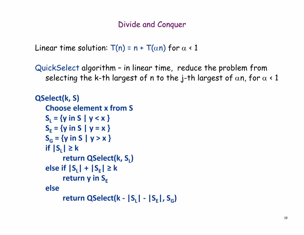
Linear time solution: T(n) = n + T(αn) for α < 1
QuickSelect algorithm – in linear time, reduce the problem from selecting the k-th largest of n to the j-th largest of αn, for α < 1
QSelect(k, S)
Choose element x from S
SL = {y in S | y < x }
SE = {y in S | y = x }
SG = {y in S | y > x }
if |SL| ≥ k
return QSelect(k, SL)
else if |SL| + |SE| ≥ k
return y in SE
else
return QSelect(k - |SL| - |SE|, SG)
19

“Choose an element x”: Random Selection
Ideally, we would choose an x in the middle, to reduce both sets in half and guarantee progress. But it’s enough to choose x at random
Consider a call to QSelect(k, S), and let S’ be the elements passed to the recursive call.
With probability at least ½, |S’| < ¾|S|
⇒ On average only 2 recursive calls before the size of S’ is at most 3n/4
bad x bad xgood x good x
elements of S listed in sorted order20

Expected runtime is O(n)
Given x, one pass over S to determine SL, SE, and SG and their sizes: cn time.
� Expect 2cn cost before size of S’ drops to at most 3|S|/4
Let T(n) be the expected running time: T(n) ≤ T(3n/4) + 2cn
By Master’s Theorem, T(n) = O(n)
Making the algorithm deterministic
� In O(n) time, find an element that guarantees that the larger set in the split has size at most ¾ n
� BFPRT (Blum-Floyd-Pratt-Rivest-Tarjan) Algorithm
21

22
Quicksort
Sorting. Given a set of n distinct elements S, rearrange them in
ascending order.
Remark. Can implement in-place.
RandomizedQuicksort(S) {
if |S| = 0 return
choose a splitter ai ∈∈∈∈ S uniformly at random
foreach (a ∈∈∈∈ S) {
if (a < ai) put a in S-
else if (a > ai) put a in S+
}
RandomizedQuicksort(S-)
output aiRandomizedQuicksort(S+)
}
O(log n) extra space

23
Quicksort
Running time.
� [Best case.] Select the median element as the splitter: quicksort
makes Θ(n log n) comparisons.
� [Worst case.] Select the smallest element as the splitter:
quicksort makes Θ(n2) comparisons.
Randomize. Protect against worst case by choosing splitter at random.
Intuition. If we always select an element that is bigger than 25% of
the elements and smaller than 25% of the elements, then quicksort
makes Θ(n log n) comparisons.
Notation. Label elements so that x1 < x2 < … < xn.

Count comparisons
ai, aj – elements in positions i and j in the final sorted list. pij the probability that ai and aj are compared
Expected number of comparisons: Σi<j pij
Prob ai and aj are compared:
� If ai and aj are compared then it must be during the call when they end up in different subproblems
- Before that, they aren’t compared to each other- After they aren’t compared to each other
� During this step they are only compared if one of them is the pivot
� Since all elements between ai and aj are also in the subproblemthis is 2 out of at least j-i+1 choices
Lemma: Pij ≤ 2/(j – i + 1)
Expected run time for QuickSort:“Global analysis”
24

25
Theorem. Expected # of comparisons is O(n log n).
Pf.
Theorem. [Knuth 1973] Stddev of number of comparisons is ~ 0.65n.
Ex. If n = 1 million, the probability that randomized quicksort takes
less than 4n ln n comparisons is at least 99.94%.
Chebyshev's inequality. Pr[|X - µ| ≥ kδ] ≤ 1 / k2.
Quicksort: Expected Number of Comparisons
2
j− i+1 = 2
1
jj=2
i
∑i=1
n
∑1≤ i < j ≤ n
∑ ≤ 2n1
jj=1
n
∑ ≈ 2n1
xdx
x=1
n
∫ = 2n lnn
probability that i and j are compared

5.4 Closest Pair of Points

27
Closest Pair of Points
Closest pair. Given n points in the plane, find a pair with smallest
Euclidean distance between them.
Fundamental geometric primitive.
� Graphics, computer vision, geographic information systems,
molecular modeling, air traffic control.
� Special case of nearest neighbor, Euclidean MST, Voronoi.
Brute force. Check all pairs of points p and q with Θ(n2) comparisons.
1-D version. O(n log n) easy if points are on a line.
Assumption. No two points have same x coordinate.
to make presentation cleaner
fast closest pair inspired fast algorithms for these problems
28
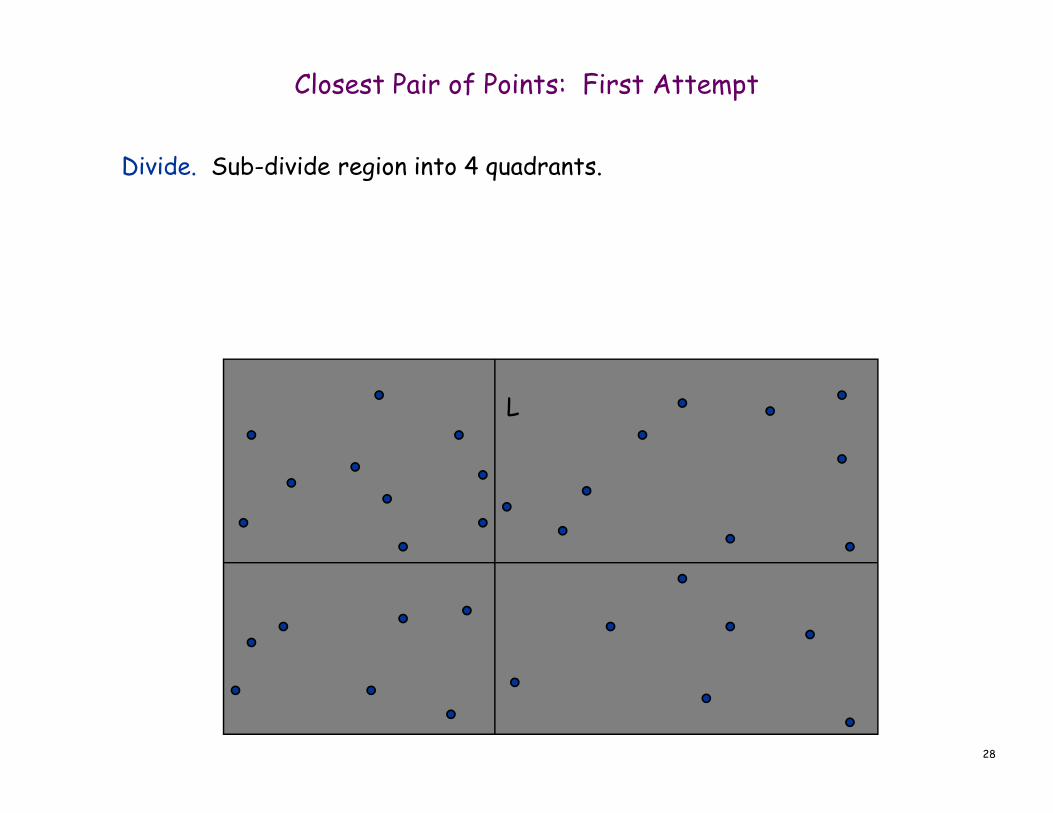
Closest Pair of Points: First Attempt
Divide. Sub-divide region into 4 quadrants.
L

29
Closest Pair of Points: First Attempt
Divide. Sub-divide region into 4 quadrants.
Obstacle. Impossible to ensure n/4 points in each piece.
L

30
Closest Pair of Points
Algorithm.
� Divide: draw vertical line L so that roughly ½n points on each side.
L

31
Closest Pair of Points
Algorithm.
� Divide: draw vertical line L so that roughly ½n points on each side.
� Conquer: find closest pair in each side recursively.
12
21
L

32
Closest Pair of Points
Algorithm.
� Divide: draw vertical line L so that roughly ½n points on each side.
� Conquer: find closest pair in each side recursively.
� Combine: find closest pair with one point in each side.
� Return best of 3 solutions.
12
218
L
seems like Θ(n2)

33
Closest Pair of Points
Find closest pair with one point in each side, assuming that distance < δ.
12
21
δ = min(12, 21)
L

34
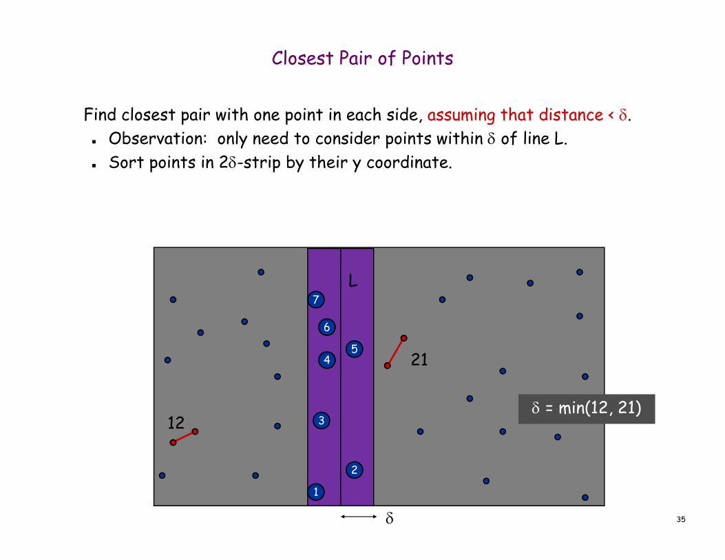
Closest Pair of Points
Find closest pair with one point in each side, assuming that distance < δ.
� Observation: only need to consider points within δ of line L.
12
21
δ
L
δ = min(12, 21)
35
12
21
1
2
3
45
6
7
δ
Closest Pair of Points
Find closest pair with one point in each side, assuming that distance < δ.
� Observation: only need to consider points within δ of line L.
� Sort points in 2δ-strip by their y coordinate.
L
δ = min(12, 21)

36
12
21
1
2
3
45
6
7
δ
Closest Pair of Points
Find closest pair with one point in each side, assuming that distance < δ.
� Observation: only need to consider points within δ of line L.
� Sort points in 2δ-strip by their y coordinate.
� Only check distances of those within 11 positions in sorted list!
L
δ = min(12, 21)

37
Closest Pair of Points
Def. Let si be the point in the 2δ-strip, with
the ith smallest y-coordinate.
Claim. If |i – j| ≥ 12, then the distance between
si and sj is at least δ.
Pf.
� No two points lie in same ½δ-by-½δ box.
� Two points at least 2 rows apart
have distance ≥ 2(½δ). ▪
Corollary For each point si, we only need to
check its distance to the 11 points that
precedes it in the y-coordinate order.
Fact. Still true if we replace 11 with 6.
δ
27
2930
31
28
26
25
δ
½δ
2 rows½δ
½δ
39
i
j

38
Closest Pair Algorithm
Closest-Pair(p1, …, pn) {
Compute separation line L such that half the points
are on one side and half on the other side.
δδδδ1 = Closest-Pair(left half)
δδδδ2 = Closest-Pair(right half)
δδδδ = min(δδδδ1, δδδδ2)
Delete all points further than δδδδ from separation line L
Sort remaining points by y-coordinate.
Scan points in y-order and compare distance between
each point and next 11 neighbors. If any of these
distances is less than δδδδ, update δδδδ.
return δδδδ.}
O(n log n)
2T(n / 2)
O(n)
O(n log n)
O(n)

39
Closest Pair of Points: Analysis
Running time.
Q. Can we achieve O(n log n)?
A. Yes. Don't sort points in strip from scratch each time.
� Each recursive returns two lists: all points sorted by y coordinate,
and all points sorted by x coordinate.
� Sort by merging two pre-sorted lists.
T(n) ≤ 2T n /2( ) + O(n) ⇒ T(n) = O(n logn)
T(n) ≤ 2T n /2( ) + O(n logn) ⇒ T(n) = O(n log2 n)

5.5 Integer Multiplication

41
Integer Arithmetic
Add. Given two n-digit integers a and b, compute a + b.
� O(n) bit operations.
Multiply. Given two n-digit integers a and b, compute a × b.
� Brute force solution: Θ(n2) bit operations.
1
1
0
0
0
1
1
1
0
0
1
1
1
1
0
0
1
1
1
1
0
1
0
1
00000000
01010101
01010101
01010101
01010101
01010101
00000000
0100000000001011
1
0
1
1
1
1
1
0
0
*
1
011 1
110 1+
010 1
111
010 1
011 1
100 0
10111
Add
Multiply

Multiplying Faster
If you analyze our usual grade school algorithm for multiplying numbers
� Θ(n2) time� On real machines each “digit” is, e.g., 32 bits long but still get
Θ(n2) running time with this algorithm when run on n-bit multiplication
We can do better!� We’ll describe the basic ideas by multiplying polynomials
rather than integers� Advantage is we don’t get confused by worrying about carries
at first
42

Notes on Polynomials
These are just formal sequences of coefficients� when we show something multiplied by xk it just means
shifted k places to the left – basically no work
Usual polynomial multiplication
4x2 + 2x + 2
x2 - 3x + 1
4x2 + 2x + 2
-12x3 - 6x2 - 6x
4x4 + 2x3 +2x2
4x4 -10x3 +0x2 - 4x + 2
43

Polynomial Multiplication
Given:� Degree n-1 polynomials P and Q
– P = a0 + a1 x + a2 x2 + … + an-2xn-2 + an-1xn-1
– Q = b0 + b1 x+ b2 x2 + … + bn-2xn-2 + bn-1xn-1
Compute:� Degree 2n-2 Polynomial P Q
� P Q = a0b0 + (a0b1+a1b0) x + (a0b2+a1b1 +a2b0) x2 +...+
(an-2bn-1+an-1bn-2) x2n-3 + an-1bn-1 x2n-2
Obvious Algorithm:� Compute all aibj and collect terms � Θ (n2) time
44

Naive Divide and Conquer
Assume n=2k� P = (a0 + a1 x + a2 x2 + ... + ak-2 xk-2 + ak-1 xk-1) +
(ak + ak+1 x + … + an-2xk-2 + an-1xk-1) xk
= P0 + P1 xk where P0 and P1 are degree k-1 polynomials
� Similarly Q = Q0 + Q1 xk
� P Q = (P0+P1xk)(Q0+Q1xk) = P0Q0 + (P1Q0+P0Q1)xk + P1Q1x2k
� 4 sub-problems of size k=n/2 plus linear combining
T(n)=4⋅T(n/2)+cn Solution T(n) = Θ(n2)
45
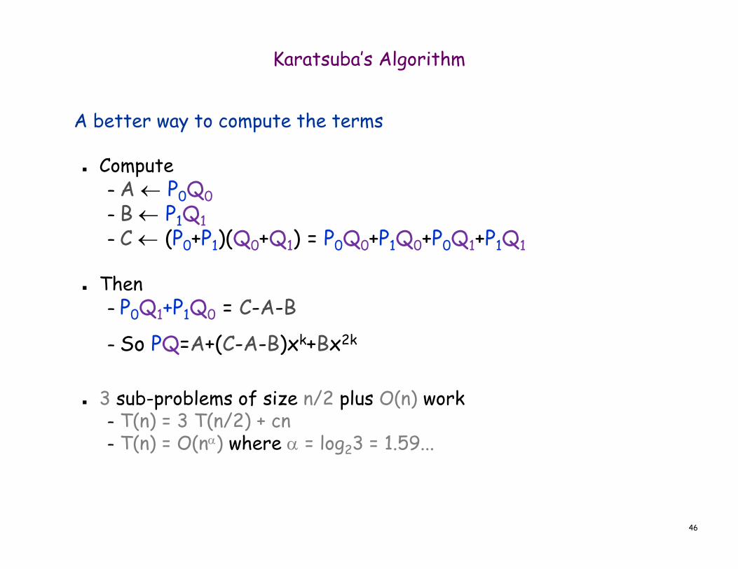
Karatsuba’s Algorithm
A better way to compute the terms
� Compute – A ← P0Q0
– B ← P1Q1
– C ← (P0+P1)(Q0+Q1) = P0Q0+P1Q0+P0Q1+P1Q1
� Then– P0Q1+P1Q0 = C-A-B
– So PQ=A+(C-A-B)xk+Bx2k
� 3 sub-problems of size n/2 plus O(n) work– T(n) = 3 T(n/2) + cn– T(n) = O(nα) where α = log23 = 1.59...
46

Karatsuba’s algorithm and evaluation and interpolation
Karatsuba’s algorithm can be thought of as a way of multiplying degree 1 polynomials (which have 2 coefficients) using fewer multiplications
� PQ=(P0+P1z)(Q0+Q1z)= P0Q0 + (P1Q0+P0Q1)z + P1Q1z2
� Evaluate at 0,1,-1 (Could also use other points)
– A = P(0)Q(0)= P0Q0
– C = P(1)Q(1)=(P0+P1)(Q0+Q1)– D = P(-1)Q(-1)=(P0 -P1)(Q0 -Q1)
47

Multiplication
Polynomials
� Naïve: Θ(n2)� Karatsuba: Θ(n1.59…)� Best known: Θ(n log n)
– "Fast Fourier Transform“– FFT widely used for signal processing
Integers� Similar, but some ugly details re: carries, etc. gives Θ(n log n
loglog n), – mostly unused in practice except for symbolic manipulation
systems like Maple
48

Matrix Multiplication

+++++++++
+++++++++
+++++++++
+++++++++
=
444434432442144142443243224212414144314321421141
443434332432143142343233223212314134313321321131
442434232422142142243223222212214124312321221121
441434132412141142143213221212114114311321121111
babababababababababababa
babababababababababababa
babababababababababababa
babababababababababababa
o
o
o
o
Multiplying Matrices
•
44434241
34333231
24232221
14131211
44434241
34333231
24232221
14131211
bbbb
bbbb
bbbb
bbbb
aaaa
aaaa
aaaa
aaaa
50

Multiplying Matrices
for i=1 to n
for j=1 to n
C[i,j]←0
for k=1 to n
C[i,j]=C[i,j]+A[i,k]⋅B[k,j]
endfor
endfor
endfor
51
n3 multiplications, n3-n2 additions

Multiplying Matrices
•
44434241
34333231
24232221
14131211
44434241
34333231
24232221
14131211
bbbb
bbbb
bbbb
bbbb
aaaa
aaaa
aaaa
aaaa
+++++++++
+++++++++
+++++++++
+++++++++
=
444434432442144142443243224212414144314321421141
443434332432143142343233223212314134313321321131
442434232422142142243223222212214124312321221121
441434132412141142143213221212114114311321121111
babababababababababababa
babababababababababababa
babababababababababababa
babababababababababababa
o
o
o
o
52

Multiplying Matrices
•
44434241
34333231
24232221
14131211
44434241
34333231
24232221
14131211
bbbb
bbbb
bbbb
bbbb
aaaa
aaaa
aaaa
aaaa
+++++++++
+++++++++
+++++++++
+++++++++
=
444434432442144142443243224212414144314321421141
443434332432143142343233223212314134313321321131
442434232422142142243223222212214124312321221121
441434132412141142143213221212114114311321121111
babababababababababababa
babababababababababababa
babababababababababababa
babababababababababababa
o
o
o
o
53

Multiplying Matrices
•
44434241
34333231
24232221
14131211
44434241
34333231
24232221
14131211
bbbb
bbbb
bbbb
bbbb
aaaa
aaaa
aaaa
aaaa
+++++++++
+++++++++
+++++++++
+++++++++
=
444434432442144142443243224212414144314321421141
443434332432143142343233223212314134313321321131
442434232422142142243223222212214124312321221121
441434132412141142143213221212114114311321121111
babababababababababababa
babababababababababababa
babababababababababababa
babababababababababababa
o
o
o
o
A11 A12
A21
A11B12+A12B22
A22
A11B11+A12B21
B11 B12
B21 B22
A21B12+A22B22A21B11+A22B21
54

Simple Divide and Conquer
T(n) = 8T(n/2) + 4(n/2)2 = 8T(n/2) + n2
� 8>22 so T(n) is
A11 A12
A21
A11B12+A12B22
A22
A11B11+A12B21
B11 B12
B21 B22
A21B12+A22B22A21B11+A22B21
=
b 2log a log 8 3( ) ( ) ( )= =Θ Θ ΘΘ Θ ΘΘ Θ ΘΘ Θ Θn n n55

Strassen’s Divide and Conquer Algorithm
Strassen’s algorithm
� Multiply 2x2 matrices using 7 instead of 8 multiplications (and lots more than 4 additions)
� T(n)= 7 T(n/2) + cn2
– 7>22 so T(n) is Θ(n ) which is O(n2.81…)
� Fastest algorithms theoretically use O(n2.373) time– not practical but Strassen’s is practical provided
calculations are exact and we stop recursion when matrix has size about 100 (maybe 10)
log27
56

The algorithm
P1←A12(B11+B21); P2←A21(B12+B22)
P3←(A11 - A12)B11; P4←(A22 - A21)B22
P5←(A22 - A12)(B21 - B22)
P6←(A11 - A21)(B12 - B11)
P7← (A21 - A12)(B11+B22)
C11←P1+P3 ; C12←P2+P3+P6 - P7
C21←P1+P4+P5+P7 ; C22←P2+P4
7 multiplications.18 = 10 + 8 additions (or subtractions).
57

58
Fast Matrix Multiplication in Practice
Implementation issues.
� Sparsity.
� Caching effects.
� Numerical stability.
� Odd matrix dimensions.
� Crossover to classical algorithm around n = 128.
Common misperception: "Strassen is only a theoretical curiosity."
� Advanced Computation Group at Apple Computer reports 8x speedup
on G4 Velocity Engine when n ~ 2,500.
� Range of instances where it's useful is a subject of controversy.
Remark. Can "Strassenize" Ax=b, determinant, eigenvalues, and other
matrix ops.

59
Fast Matrix Multiplication in Theory
Q. Multiply two 2-by-2 matrices with only 7 scalar multiplications?
A. Yes! [Strassen, 1969]
Q. Multiply two 2-by-2 matrices with only 6 scalar multiplications?
A. Impossible. [Hopcroft and Kerr, 1971]
Q. Two 3-by-3 matrices with only 21 scalar multiplications?
A. Also impossible.
Decimal wars.
� December, 1979: O(n2.521813).
� January, 1980: O(n2.521801).
Θ(n log3 21) =O(n 2.77 )
Θ(n log2 6) =O(n 2.59 )
Θ(n log2 7 ) =O(n 2.81)

60
Fast Matrix Multiplication in Theory
Until Oct 2011. O(n2.376) [Coppersmith-Winograd, 1987.]
Best known. O(n2.373) [V . Williams, Nov 2011]
Conjecture. O(n2+ε) for any ε > 0.
Caveat. not practical but Strassen’s is practical provided calculations are exact and we stop recursion when matrix has size about 100 (maybe 10)