Increasing Network Resiliency by OptimallyAssigning Diverse Variants to Routing Nodes

Andrew Newell1, Daniel Obenshain2, Thomas Tantillo2, Cristina Nita-Rotaru1, and Yair Amir2

1Department of Computer Science at Purdue University{newella,crisn}@cs.purdue.edu

2Department of Computer Science at Johns Hopkins University{dano,tantillo,yairamir}@cs.jhu.edu

Technical Report TR-13-002, Department of Computer Science, Purdue UniversityApril 24 2013

Abstract—Networks with homogeneous routing nodes areconstantly at risk as any vulnerability found against a node couldbe used to compromise all nodes. Introducing diversity amongnodes can be used to address this problem. With few variants,the choice of assignment of variants to nodes is critical to theoverall network resiliency.

We present the Diversity Assignment Problem (DAP), theassignment of variants to nodes in a network, and we show howto compute the optimal solution in medium-size networks. Wealso present a greedy approximation to DAP that scales well tolarge networks. Our solution shows that a high level of overallnetwork resiliency can be obtained even from variants that areweak on their own.

For real-world systems that grow incrementally over time, weprovide an online version of our solution. Lastly, we provide avariation of our solution that is tunable for specific applications(e.g., BFT).

I. INTRODUCTION

Networks with homogeneous routing nodes are constantlyat risk as any vulnerability found against a single routingnode could be used to compromise all nodes. Diversity canbe employed at various levels on the routing nodes to addressthis problem by improving resiliency against different classesof attacks. In this work, we base resiliency on the number ofsurviving client-to-client connections offered by the networkwhen under attack. Diversifying the operating system providesprotection against common types of attacks that target operat-ing system vulnerabilities [1]; utilizing multi-variant program-ming protects against programming vulnerabilities or logicalprogramming errors [2], [3]; using different administrativepersonnel mitigates social engineering or insider attacks [4].However, there are only a limited number of operating systems,software versions, and personnel to utilize as diverse variants.So then, how does one assign these limited number of diversevariants to the routing nodes in the network to achieve optimalresiliency?

Initially, we assumed that a random assignment of afew diverse variants would perform well. However, we weresurprised to find that a random assignment performs ratherpoorly, in many cases providing less resiliency than using thebest single variant at all routing nodes, and occasionally evenless resiliency than using the worst single variant at all routing

nodes. Clearly, a better approach is necessary to realize thebenefits of diversity.

Our interest in this question arose from constructing a cloudservice over a global network of data centers [5]. We needed tohave an intrusion-tolerant infrastructure in order to monitor andcontrol the cloud even in the case of sophisticated intrusions.While designing intrusion-tolerant protocols for messaging andmaintaining consistent state, we realized that without diversityall the nodes could be compromised by a single vulnerability.Inspired by [1], we were especially interested in diversifyingthe operating system (e.g., Linux, MacOS, and FreeBSD). Theadditional overhead of managing multiple operating systemswithin the cloud infrastructure led us to consider only a smallnumber of variants to create diversity.

In this paper, we demonstrate that the way diverse variantsare assigned across the network (i.e., which variant is assignedto which routing node) is of utmost importance to the overallnetwork resiliency when the number of variants is smaller thanthe number of routing nodes in the network. To our knowledge,this work is the first to study the impact of variant assignmentto routing nodes on overall network resiliency.

We present a novel problem, the Diversity AssignmentProblem (DAP), which specifies how to optimize overallnetwork resiliency when placing diverse variants that arecompromised independently at routing nodes. While DAP isNP-Hard, we show that it is feasible to solve it optimally on avariety of medium-size random network graphs. We also showan efficient algorithm that approximates DAP well for largergraphs, incurring a relatively small resiliency cost comparedwith the optimal solution.

To check the applicability of our approach in a real-worldsetting, we obtained a network graph representative of theglobal overlay topology used by the above cloud service. Eventhough this topology was constructed with high availability asthe goal (rather than intrusion-tolerance), the optimal variantassignment solution to the DAP ensures a system resiliencythat is significantly higher than the resiliency achieved by anyof the individual variants.

In real-life settings, routing nodes may be added from timeto time to meet increasing system demands. Calculating anoptimal solution for the extended network is certainly feasible.

However, that solution is likely to require variant re-assignmentfor many of the existing routing nodes, which may not befeasible in a 24/7 service as downtime for re-configuring nodesis unacceptable. We present an online version of DAP thatfinds the optimal incremental assignment. When applied tothe mentioned global topology, we discover that an importanttrade-off exists between the resiliency the system achieves andhow often the network changes.

We initially choose an application agnostic metric fornetwork resiliency that captures the expected client-to-clientconnectivity between all pairs. We investigate the advantagesof considering the specific resiliency needs defined by thenature of a distributed application running at the clients.Specifically, we show how to find the optimal assignmentfor the underlying network supporting the Byzantine Fault-Tolerant Protocol (BFT) [6]. When applied to the mentionedglobal topology, we found that an assignment that is tailoredto BFT requirements can provide higher resiliency than anassignment that focuses on general network resiliency obtainedby maximizing the expected client-to-client connectivity.

When studying DAP, we learned three key points that arerelevant to any application of limited diversity that aims toincrease network resiliency:

- A high level of overall network resiliency can beobtained even from variants that are weak on theirown. Despite the variants being compromised (inde-pendently) with a relatively high probability, they arecompromised in different ways. Carefully assigningvariants to routing nodes allows surviving subsets ofthe network to still remain highly connected.

- The simplest and seemingly practical approach of justassigning variants randomly offers very low resiliencycompared to the optimal assignment. Additionally, inmany random placements we found that the resiliencyof the network is actually worse than if no diversityassignment were used at all.

- While optimizing expected client-to-client connectiv-ity provides a good measure for the resiliency of thenetwork to intrusions, considering application-specificconnectivity requirements may lead to a differentassignment that maximizes overall system resiliency(as opposed to network resiliency) for that applicationon that network.

The contributions of this paper are as follows:

• We introduce the Diversity Assignment Problem(DAP).

• We formulate the DAP using mixed integer program-ming (MIP) [7] and find the optimal solution onrandom graphs constructed in a manner reminiscent ofreal overlay topologies. To support larger graphs, weextend this formulation to a fast greedy approximationand demonstrate results that are relatively close to theoptimal solution in such larger graphs.

• We analyze the impact of diversity on a real cloudoverlay topology and extend our approach to supportadding routing nodes to the graph in an online mannerto address increased client demand.

• We extend our approach to optimize network re-siliency for a given application’s demands, rather thanfor overall expected client-to-client connectivity, tomaximize system resiliency.

The rest of the paper is organized as follows. Section IIdescribes our network and attacker models. Section III presentsthe general DAP along with an optimal solution. Section IVdescribes and evaluates a greedy approximation algorithmto solve DAP in larger topologies. Section V shows howresiliency is affected in dynamic topology scenarios. Sec-tion VI shows the increased advantage of performing diversityassignment with client application knowledge. Section VII listswork related to ours. Section VIII concludes this work.

II. MODEL

We describe the model of the network and attacker whichwe consider in this work. These models are quite general asour approaches can be applied in various networking contextswith various of diversity techniques. Our motivation startedwith a scenario of cloud services being provided over a globalnetwork of datacenters while diversifying operating systemsfor improved resilience, but we noticed that the core problemis general to any network.

A. Network model

We assume a network topology of routing nodes thatprovide communication to clients. We assume no controlover the structure of the network topology as this is fixedbased on the constraints of the networking context. In anoverlay routing context, network links impose overhead tocontinuously monitor their latency and loss characteristics,thus the degree at each node must be limited while ensuringthe entire network is still well connected. Alternatively, in awireless context, network links are limited by the physicalbroadcast range of each node. We assume that we have a setof diverse variants and can configure each routing node with asingle variant. Our network goals are to maximize the numberof client connections or an application-specific communicationrequirement of the clients.

B. Attacker model

We assume that there is no way to configure a routingnode that meets our network needs while being completelyinvulnerable to attacker attempts of compromise. Thus, weadopt a probabilistic attacker model that captures the followingimportant resilience property of diversity we wish to leverage:even though we do not have access to a variant that cannotbe compromised, we do have access to variants that arecompromised in different ways. We assign a probability thatan attacker is able to both find a vulnerability and create asuccessful exploit against a variant within a given time period,and then any routing node in the network with this variant willbecome compromised. As our probabilities are with respectto a certain time frame, a full long-term system would needmechanisms to detect and recover compromised variants, andwe consider such mechanisms as outside the scope of thiscurrent work. Our probabilistic model of compromise offersa useful way to reason about an attacker’s capabilities andmeasure a network’s resilience. Even in realistic scenarioswhere an attacker is not modeled well probabilistically, we are

still raising the bar for the attacker to ensure the attacker mustfind vulnerabilities and create exploits for different variants ofrouting nodes.

We do assume a byzantine tolerant routing protocol is usedfor routing to ensure that communication can occur betweentwo clients as long as a honest path of routing nodes exists.

III. DIVERSITY ASSIGNMENT

In this section we present the Diversity Assignment Prob-lem (DAP). DAP describes how to assign diversity to routingnodes in order to maximize the probability of each client pairbeing connected. We then describe existing Mixed IntegerProgramming (MIP) techniques and how these can be usedto solve DAP. Lastly, we show the effectiveness of thistechnique on a realistic case study topology when comparedwith randomly assigning diversity.

A. Diversity Assignment Problem (DAP)

We consider a network consisting of a set of nodes N and aset of clients M . A set of connections are defined among thesenodes, so we can represent a network as a graph such as theone in Figure 1. Each routing node is assigned a variant fromthe set of variants V , so there are |V ||N | possible assignments.We denote an assignment of one variant for each node as A.Note that |V | < |N |. Each variant vk ∈ V is associated witha compromise event ek in the set of all compromise eventsE, so |E| = |V |. The probability of ek occurring is P (ek).These events of compromise are independent,∗ so for any twocompromise events ek′ and ek′′ the following holds P (ek′ ∩ek′′) = P (ek′) ∗ P (ek′′).

We measure the goodness of an assignment of variantswith the metric expected client connectivity. This metric isthe expected value of the proportion of client pairs that areconnected. To compute this value we consider the set ofall possible combinations of compromise events C where|C| = 2|E| (C is the powerset [8] of E). An element c ∈ C is asubset of the compromise events, E, and corresponds to thosecompromise events occurring while any other compromiseevents do not occur. We can compute the proportion of clientsconnected given that those variants are compromised. We con-sider two clients to be connected if a path of uncompromisednodes exists between them.

Our goal is to maximize the expected client connectivityof a graph by strategically assigning variants. We call thisproblem the Diversity Assignment Problem.

Definition 1: The Diversity Assignment Problem is to findthe assignment of variants to nodes which maximizes theexpected client connectivity. First, for a given assignment Aand set of compromised variant events c ∈ C, we define aconnectivity function fA,c(a, b) between two clients a and b

∗We make an assumption of independence among compromise events inthis work as this simplifies the presentation of the fundamental ideas inthis work. However, as long as compromise events are not highly positivelycorrelated (i.e., when one compromise event occurs then others are highlylikely to happen), then all of our techniques and results still hold even thoughcompromise events may not be completely independent.

(a) (b)

Fig. 1. Example of two assignments on the same topology where routingnodes are circles and clients are squares. We show two possibilities fordiversity assignment to nodes where the two variants are blue (dark) whichhas a 0.1 probability of being compromised and yellow (light) which has a0.15 probability of compromise. (a) Diversity assignment with 0.838 expectedclient connectivity. Notice that only one client pair is connected if eitherblue or yellow is compromised. (b) Superior diversity assignment that has0.957 expected client connectivity. Notice that three client pairs are connectedif yellow is compromised and two client pairs are connected if blue iscompromised.

as:

fA,c(a, b) =

(|M |

2

)−1if clients a and b are connectedby a set of uncompromised nodes

0 otherwise

Then, the expected client connectivity is:

E

∑{a,b∈M :a<b}

fA,c(a, b)

=

∑c∈C

∏ek∈c

P (ek)∏ek /∈c

(1− P (ek))

∗

∑{a,b∈M :a<b}

fA,c(a, b)

The Diversity Assignment Problem is:

argmaxA

E ∑{a,b∈M :a<b}

fA,c(a, b)

Theorem 1: The Diversity Assignment Problem is NP-

Hard with two or more variants.

Proof: The proof is in Appendix IX.

As an illustrative example of the meaning of DAP we giveFigure 1 as an example topology graph. Figures 1(a) & 1(b)show two ways to assign variants in this graph. Figure 1(b)is the superior assignment as more client pairs are connectedgiven that a single variant is compromised. The superiorityof this assignment is also reflected by the expected clientconnectivity values. This section is focused on finding theoptimal variant assignment for a topology.

B. MIP approach to DAP

Despite DAP being NP-Hard, many real-world networktopologies are of limited size, so finding the optimal solutionis of practical interest. To find the optimal solution, we choseto formulate the problem as a MIP and utilize an existingcommercial solver, CPLEX [9]. A MIP is a linear program with

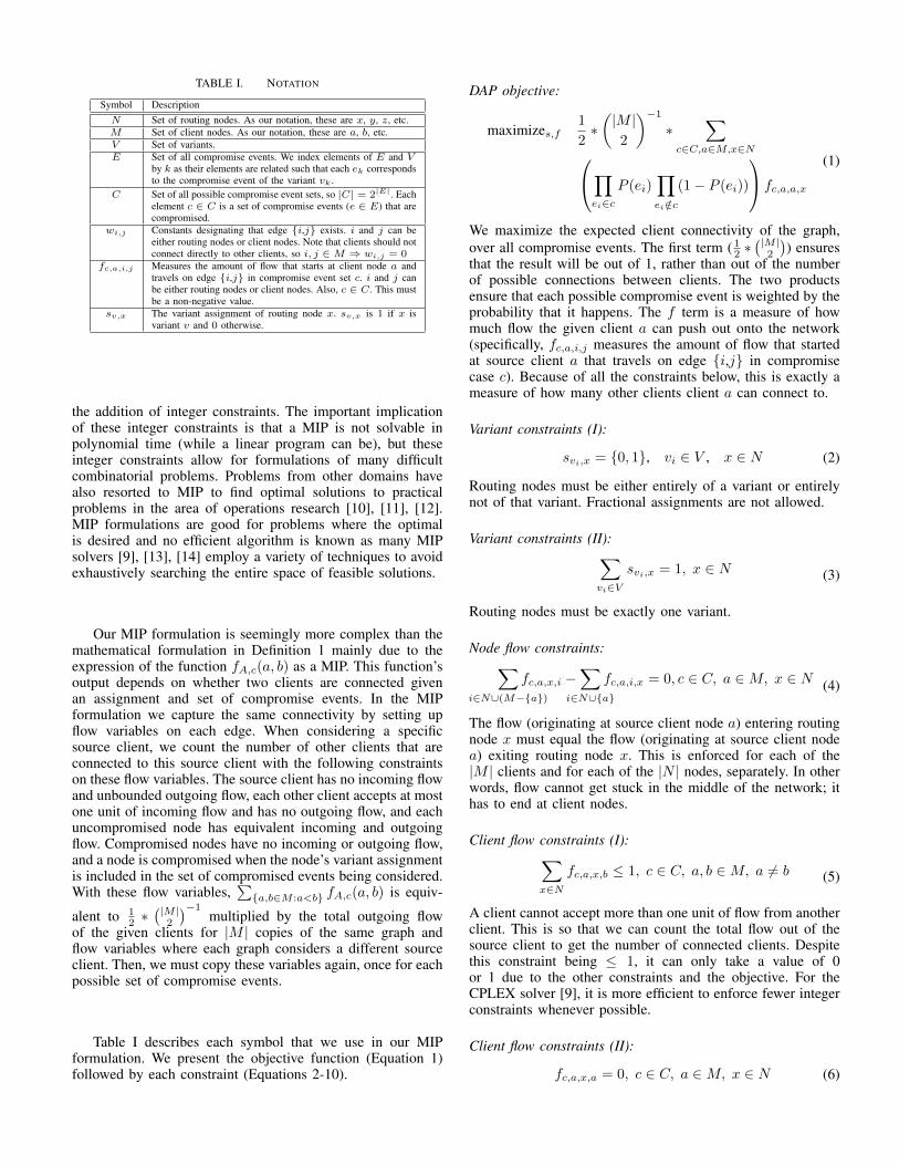
TABLE I. NOTATION

Symbol DescriptionN Set of routing nodes. As our notation, these are x, y, z, etc.M Set of client nodes. As our notation, these are a, b, etc.V Set of variants.E Set of all compromise events. We index elements of E and V

by k as their elements are related such that each ek correspondsto the compromise event of the variant vk .

C Set of all possible compromise event sets, so |C| = 2|E|. Eachelement c ∈ C is a set of compromise events (e ∈ E) that arecompromised.

wi,j Constants designating that edge {i,j} exists. i and j can beeither routing nodes or client nodes. Note that clients should notconnect directly to other clients, so i, j ∈M ⇒ wi,j = 0

fc,a,i,j Measures the amount of flow that starts at client node a andtravels on edge {i,j} in compromise event set c. i and j canbe either routing nodes or client nodes. Also, c ∈ C. This mustbe a non-negative value.

sv,x The variant assignment of routing node x. sv,x is 1 if x isvariant v and 0 otherwise.

the addition of integer constraints. The important implicationof these integer constraints is that a MIP is not solvable inpolynomial time (while a linear program can be), but theseinteger constraints allow for formulations of many difficultcombinatorial problems. Problems from other domains havealso resorted to MIP to find optimal solutions to practicalproblems in the area of operations research [10], [11], [12].MIP formulations are good for problems where the optimalis desired and no efficient algorithm is known as many MIPsolvers [9], [13], [14] employ a variety of techniques to avoidexhaustively searching the entire space of feasible solutions.

Our MIP formulation is seemingly more complex than themathematical formulation in Definition 1 mainly due to theexpression of the function fA,c(a, b) as a MIP. This function’soutput depends on whether two clients are connected givenan assignment and set of compromise events. In the MIPformulation we capture the same connectivity by setting upflow variables on each edge. When considering a specificsource client, we count the number of other clients that areconnected to this source client with the following constraintson these flow variables. The source client has no incoming flowand unbounded outgoing flow, each other client accepts at mostone unit of incoming flow and has no outgoing flow, and eachuncompromised node has equivalent incoming and outgoingflow. Compromised nodes have no incoming or outgoing flow,and a node is compromised when the node’s variant assignmentis included in the set of compromised events being considered.With these flow variables,

∑{a,b∈M :a<b} fA,c(a, b) is equiv-

alent to 12 ∗

(|M |2

)−1multiplied by the total outgoing flow

of the given clients for |M | copies of the same graph andflow variables where each graph considers a different sourceclient. Then, we must copy these variables again, once for eachpossible set of compromise events.

Table I describes each symbol that we use in our MIPformulation. We present the objective function (Equation 1)followed by each constraint (Equations 2-10).

DAP objective:

maximizes,f1

2∗(|M |

2

)−1∗

∑c∈C,a∈M,x∈N∏

ei∈cP (ei)

∏ei /∈c

(1− P (ei))

fc,a,a,x

(1)

We maximize the expected client connectivity of the graph,over all compromise events. The first term ( 12 ∗

(|M |2

)) ensures

that the result will be out of 1, rather than out of the numberof possible connections between clients. The two productsensure that each possible compromise event is weighted by theprobability that it happens. The f term is a measure of howmuch flow the given client a can push out onto the network(specifically, fc,a,i,j measures the amount of flow that startedat source client a that travels on edge {i,j} in compromisecase c). Because of all the constraints below, this is exactly ameasure of how many other clients client a can connect to.

Variant constraints (I):

svi,x = {0, 1}, vi ∈ V , x ∈ N (2)

Routing nodes must be either entirely of a variant or entirelynot of that variant. Fractional assignments are not allowed.

Variant constraints (II):∑vi∈V

svi,x = 1, x ∈ N (3)

Routing nodes must be exactly one variant.

Node flow constraints:∑i∈N∪(M−{a})

fc,a,x,i −∑

i∈N∪{a}

fc,a,i,x = 0, c ∈ C, a ∈M, x ∈ N (4)

The flow (originating at source client node a) entering routingnode x must equal the flow (originating at source client nodea) exiting routing node x. This is enforced for each of the|M | clients and for each of the |N | nodes, separately. In otherwords, flow cannot get stuck in the middle of the network; ithas to end at client nodes.

Client flow constraints (I):∑x∈N

fc,a,x,b ≤ 1, c ∈ C, a, b ∈M, a 6= b (5)

A client cannot accept more than one unit of flow from anotherclient. This is so that we can count the total flow out of thesource client to get the number of connected clients. Despitethis constraint being ≤ 1, it can only take a value of 0or 1 due to the other constraints and the objective. For theCPLEX solver [9], it is more efficient to enforce fewer integerconstraints whenever possible.

Client flow constraints (II):

fc,a,x,a = 0, c ∈ C, a ∈M, x ∈ N (6)

Traffic cannot start and end at the same client. In other words,a client cannot send to itself. Note that {x, a} is any incomingedge into a.

Client flow constraints (III):

fc,a,b,x = 0, c ∈ C, a, b ∈M, x ∈ N, a 6= b (7)

A destination client cannot send out flow. So, flow cannot usea client to reach other clients.

Topology constraints:

fc,a,i,j ≤ (|M | − 1) ∗ wi,j , c ∈ C, a ∈M, i, j ∈ (N ∪M)(8)

Any pair of nodes with no edge between them (i.e., wi,j = 0)cannot have any flow directly between them. It also underlinesthe fact that up to |M |−1 units of flow originating at the sameclient can share the same edge.

Variant flow constraints (I):

fc,a,x,i ≤ (|M | − 1) ∗ minei∈C

(1− svi,x),

c ∈ C, a ∈M, x ∈ N, i ∈ N ∪M(9)

The amount of flow out of a routing node must be 0 if thatnode is compromised. It also underlines the fact that no edgecan carry more than |M | − 1 units of flow from any sourceclient node a.

Variant flow constraints (II):

fc,a,i,x ≤ (|M | − 1) ∗minei∈c

(1− svi,x),

c ∈ C, a ∈M, i ∈ N ∪M, x ∈ N(10)

The amount of flow into a node must be 0 if that node iscompromised. It also underlines the fact that no edge can carrymore than |M | − 1 units of flow from any source client nodea.

C. DAP on the case study topology

We investigate the benefit of optimal diversity assignmenton a realistic overlay network topology. The topology andcompromise scenario are detailed in Table II. Then, variousassignments of diversity are shown on the case study topologywith their corresponding expected client connectivity. We showassignments for DAP with increasing number of variants beingused, and we investigate random assignments as a comparisonwith the optimal solution.

For a case study topology, we took a connectivity graphfrom a cloud network provider [5]. The nodes of the graphrepresent data centers located around the globe. Each node isassigned a single variant which means that the overlay routingelement at that data center will utilize the selected variant. Theedges of the graph represent overlay connectivity used on thatcloud to connect the different data centers. This connectivityis provided by a number of Internet Service Providers ateach data center. The clients in the graph represent eitherclients external to the cloud or infrastructure components ofthe cloud. Each client has multiple connections to the cloud toavoid a single point of failure. In this example, we use threeconnections as that level of connectivity was quite prevalent

in that network. This connectivity graph was designed withresiliency in mind, and without any consideration for diversity.

We assume some hypothetical scenario with three diversevariants represented by blue (darkest), yellow (lightest), andred (medium) having a 0.1, 0.15, and 0.2 probability of beingcompromised over some arbitrary period of time, respectively.Note that this example, while simplistic, provides an interest-ing insight into the benefits and risks of diversity. †

Figure 2(a) shows the optimal solution when only a singlevariant can be used. All the nodes are assigned with the leastvulnerable variant. This corresponds to the situation where nodiversity is used. The resulting network achieves an expectedclient connectivity of 0.9.

Figure 2(b) shows the optimal solution when two variantscan be used. Each node is assigned with either of the twoleast vulnerable variants. The resulting network achieves anexpected client connectivity of 0.985. Note that this is betterthan either variant by itself.

Figure 2(c) shows the optimal solution when three variantscan be used. The resulting network achieves an expected clientconnectivity of 0.997. Notice that the optimal solution finds anassignment where any single variant is capable of connectingall clients. By adding a third, more vulnerable variant actuallymakes the system significantly more resilient.

As stated before, in this example, each client is connectedto three routing nodes. If clients do not have at least threepotential entry points into the network, then the availability ofthe connection is limited by the variants of the routing nodesthat they are connected to. For example, if each client onlyconnects to a single routing node, that connection would failif either of the entry-point routing nodes is compromised. Thisis much more likely to occur than if there are three such entry-point routing nodes for each client, requiring at least threerouting nodes to be compromised to cut the connection.

In this example, including variants that have a higherbut independent probability of being compromised improvesthe overall system resiliency. This may be counterintuitive,as adding weaker components to a system usually makesit weaker, not stronger. The independence of the differentvariants and the overall robustness of the network mean that†The purpose of these values is to give preference to one variant over

another and to quantify an estimate of the system resiliency with diversity.While we select numbers to illustrate the main concepts, the resultingassignment would not be significantly different if other values were selected.

TABLE II. NETWORK CHARACTERISTICS FOR CASE STUDYTOPOLOGY.

Symbol DescriptionN Set of 20 overlay nodes, shown in the figures as colored circles.M Set of 10 client nodes, shown in the figures as white squares.V Set of variants. v1 represented by blue, v2 represented by

yellow, and v3 represented by red. In Figure 2(a): {v1}. In Fig-ure 2(b): {v1, v2}. In Figure 2(c) and Figure 4: {v1, v2, v3}.

C Set of compromise event sets. In Figure 2(a): {{}, {v1}}.In Figure 2(b): {{}, {v1}, {v2}, {v1, v2}}. In Figure 2(c)and Figure 4: {{}, {v1}, {v2}, {v3}, {v1, v2}, {v1, v3},{v2, v3}, {v1, v2, v3}}.

wi,j Constants designating that edge {i, j} exists. These are toonumerous to be listed here, but can be observed from the figures.

E The probability of compromise events for each variant areP (e1) = .1, P (e2) = .15, P (e3) = .2.

(a) (b) (c)

Fig. 2. Optimal assignments on case study topology: (a) one variant assignment achieves 0.9 expected client connectivity, (b) two variants assignment achieves0.985 expected client connectivity, (c) three variants assignment achieves 0.997 expected client connectivity.

adding additional, more vulnerable variants makes a systemmore resilient.

As discussed earlier, random assignment could be usedinstead of the optimal MIP approach. One might expect thisapproach to do well, since randomness often helps in addingdiversity to systems. However, this does not necessarily leadto a good result. An example graph can be seen in Figure 4.This graph achieves an expected client connectivity of only0.811, much worse than any of the other three graphs. Infact, it barely outperforms the worst of the three variants.This example graph comes from the bottom 1% of possibleassignments and is given as an example of what could occurif the diversity assignment is not considered carefully.

Figure 3 is a histogram created with data from 100,000random assignments of this graph. For this data set, theminimum and maximum are 0.751 and 0.988 respectively. Themean is 0.931 and the median is 0.937. As can be seen, most ofthe random assignments perform better than if the best variantis used by itself (0.937 > 0.9). However, very few of therandom assignments come close to performing as well as theoptimal assignment found by MIP.

The optimal solution of 0.997 expected client connectivityexists while the best random solution out of the 100,000random assignment shown in Figure 3 was 0.988 expectedclient connectivity. Thus, even the best random solution outof numerous trials does not achieve the optimal solution.The probability of a client communication being broken is(1 − 0.988) = 0.012 for the best random solution comparedwith (1−0.997) = 0.003 for the optimal solution, so a client-to-client connection is broken four times less often with theoptimal assignment.

Interestingly, the difference between what the optimalsolution provides and the probability that at least one of thevariants is uncompromised provides a metric for the qualityof the connectivity resiliency of the graph.‡ Ideally, we wouldwant this distance to be zero, as in Figure 2(b) and Figure 2(c)of the provided example.

IV. SCALING DIVERSITY ASSIGNMENT

DAP is not tractable for large topologies since DAP isNP-Hard (see Theorem 1). To scale to larger topologies, wesacrifice optimality in order to ensure the algorithm completeswithin a polynomially-bounded time. In this section we presentthe Approximate DAP (A-DAP), a greedy approach to A-DAP,

‡Thanks to Bob Balzer for this observation.

0

2000

4000

6000

8000

10000

12000

0.7 0.75 0.8 0.85 0.9 0.95 1

Count

Expected client connectivity

0.9

88

0.7

51

Fig. 3. Histogram of expected client connectivity of 100,000 randomassignments, and the vertical dashed lines represent lower and upper bounds.

Fig. 4. A random assignment that achieves 0.881 expected client connectivity

Fig. 5. Greedy assignment achieves 0.992 expected client connectivity.

an example on the case study topology, and an evaluation onrandom topologies.

A. Approximate DAP (A-DAP)

A-DAP is similar to DAP, but A-DAP does not require thatthe problem be solved optimally. By relaxing this condition,we aim to find algorithms that run in polynomial time whichare able to find large values of expected client connectivity.We do not formally define any restrictions on the goodnessof the approximations as it is an open problem of whether areasonable bound can be placed on the expected client connec-tivity achieved by a deterministic polynomial time algorithm.Instead, we used random topologies to validate the goodness ofexpected client connectivities achieved by a greedy approachto A-DAP when compared with the optimal.

B. Greedy approach to A-DAP

Our greedy approach incrementally assigns nodes to vari-ants. At each incremental assignment, the algorithm consid-ers several candidate assignments and selects the one whichprovides the best immediate results. For a candidate set ofincremental assignments we consider sets of nodes whichcan connect a client pair by a variant, so we consider atmost

(|M |2

)∗ |V | candidate variant assignments. For a given

client pair and variant, we compute the minimal number ofunassigned nodes which must be assigned that variant toconnect those clients by that variant. After this computation wehave two values: the increase in expected client connectivityα and the number of newly assigned nodes β.

Given a set of candidate assignments that each have anα and β value, we select the one which maximizes α

β . It isobvious why we want to find large α values, but it is equallyimportant to ensure the β value is small as well. Smallervalues of β allow for more nodes to remain unassigned andto be used to connect more client pairs by other variants infuture assignments. This approach is analogous to the greedychoice in bin packing, as we select items with the highestpayoff versus weight ratio to ensure that items are selectedthat increase overall payoff while allowing for more items tobe picked in the future. Note, that β = 0 is a trivial casewhere the candidate is simply removed from consideration asthe client pair is already connected via the considered variant.

The pseudo-code of the algorithm is shown in Algorithm 1.Each iteration of the while loop (Line 3-19) creates a setof candidate variant assignments (Line 7), then selects thebest candidate (Line 11-15), and lastly applies the assignmentof that candidate to the topology (Line 18). This algorithmcompletes when no further client pairs can be connected bya variant, and the algorithm is guaranteed to complete in abounded number of iterations since each step connects at leastone new client pair via a variant (at most |C|∗|M |2 iterations).

C. A-DAP on the case study topology

We consider the same scenario as in Section III-C withthree variants. Figure 5 shows the assignment found by ourgreedy solution which achieves 0.992 expected client connec-tivity. Notice that all clients are connected via just the blueor yellow variants. However, two clients remain unconnectedfrom the rest if only the red variant is uncompromised. The

Algorithm 1 Greedy assignment algorithmVariables

CPVC: Client Pair and Variant CombinationsVA: Variant AssignmentDVA: Delta Variant AssignmentCG: Connectivity GainBCG: Best Connectivity GainDVA: Delta Variant AssignmentBDVA: Best Delta Variant Assignmentα: Tunable parameter which affects the trade-off be-tween increasing connectivity and minimizing the sizeof the DVA set

Functionsf(·, ·): Minimal set of unassigned overlay nodes thatmust be assigned a particular variant to connect aparticular client pairg(·): Overall connectivity for a particular variant as-signment

Algorithm1: CPVC := M ×M × V2: VA := ∅3: while CPVC 6= ∅ do4: BCG := 05: BDVA := ∅6: for all x ∈ CPVC do7: DVA := f(x,VA)8: if DVA = ∅ then9: CPVC := CPVC− x

10: else11: CG := g(VA∪DVA)−g(VA)

|DVA|α12: if CG > BCG then13: BDVA := DVA14: BCG := CG15: end if16: end if17: end for18: VA := VA ∪ DVA19: end while

optimal solution found with the MIP formulation finds anassignment which connects all clients as long as any singlevariant is uncompromised. This loss of expected client con-nectivity is due to the greedy algorithm making choices inthe early steps of the algorithm to connect clients via blueand yellow variants (the more resilient variants) which leavesfewer choices to connect clients via the red variants. Thegreedy approach for the A-DAP took 0.38 seconds to completewhile the MIP approach for the DAP took 396.13 seconds tocomplete. With far less computational requirements, the greedyalgorithm does outperform the best of the 100,000 randomassignments (0.988 client connectivity) and comes close to theoptimal solution.

D. A-DAP on random topologies

We present a methodology followed by results to answerthe following questions of interest about the performance ofthe greedy algorithm for the A-DAP:

1) How does the goodness of the assignment of the

greedy algorithm compare to other algorithms (ran-dom assignment and optimal) for the DAP on typicaltopologies?

2) How does the running time of the greedy algorithmfor the A-DAP and the MIP approach for the DAPvary with typical topologies created with differentparameters?

3) What are trends in the expected client connectivityover all the assignment algorithms when varyingtopology parameters?

We select expected client connectivity and running timeto measure for each algorithm. Expected client connectivityis a measure of how well the algorithm performs, which canbe compared with MIP’s optimal value. Running time is ameasure of how quickly the algorithm will terminate with anexpected client connectivity.

We generate random topologies in a similar way to randomwireless topologies. That is, we place the desired number ofnodes and clients randomly inside a two-dimensional box.Then, based on a density parameter, we give each node andclient a range. All nodes and client within the range havean edge between them. The density parameter is the averagenumber of nodes each node or client is connected to. Notethat client to client edges are not added. We can create manyrandom topologies given a number of nodes and a densityvalue. We chose to limit the number of nodes in order to ensurethat the optimal value could be calculated for comparison.Topologies constructed in this way are obviously representativeof wireless contexts, but they are also quite similar to overlaytopologies, because overlay topologies include many short,well-behaved links.

Given topology parameters, we create 30 random topolo-gies and run the three algorithms on these topologies. Weaverage the expected client connectivity and running timesobtained for each algorithm over the 30 runs. For the runningtime values of the MIP formulation, it is important to notethat we use the software package CPLEX with a quad-core3.4 Ghz Intel processor which does leverage all cores.

The results are shown in Figure 6. We describe how theyanswer each of the initial questions that we proposed.

Question 1. The goodness of an algorithm’s assignmentis the expected client connectivity. This is upper-bounded bythe optimal value (which the MIP approach always achieves).The greedy algorithm outperformed the random assignmentand was quite close to the optimal value, independent ofvarying either density (Figure 6(a)) or the number of nodes(Figure 6(c)).

Question 2. The running time of the greedy algorithm ison the order of milliseconds, which is barely visible whencompared to the running time of the MIP-based approach.Figure 6(b) shows the MIP approach running time for varyingdensity values. The running time is low for small densityvalues since most variant assignments result in poor expectedclient connectivity, allowing the branch-and-bound algorithmof CPLEX to avoid searching the majority of variant assign-ments. The running time is also low for high density valuessince a dense graph has many possible optimal assignmentsand the branch-and-bound algorithm can terminate early after

finding any of them. Thus, the problem is hardest for moderatedensity values. The running time of both algorithms whenvarying the size of the network is shown in Figure 6(d). TheMIP approach running time grows nearly linearly over theseinput parameters, but this relationship is potentially exponen-tial according to Theorem 1. The MIP approach running timeis still significantly greater than the greedy approach.

Question 3. The trend of expected client connectivityis similar among all three algorithms. The expected clientconnectivity increases as density increases (Figure 6(a)), whichis expected since more edges allow more possibilities forclients to become connected. The expected client connectivitydecreases as the number of nodes increases (Figure 6(c)). Bykeeping the density constant and increasing the number ofnodes, the graph becomes less connected and therefore lessresilient.

From these results we see that the greedy algorithm out-performs the random algorithm while being quite close tothe optimal solution, and the greedy algorithm is far moreefficient in terms of running time and is polynomially-boundedwhile the MIP formulation is not. Hence, on larger topologieswhere the MIP formulation cannot be computed, the greedyalgorithm is a decent substitute. Another interesting resultis that the expected client connectivity decreases with morenodes when keeping the density constant. So, the density ornode degree must increase to retain high levels of expectedclient connectivity when the number of nodes increases in thetopology.

V. DIVERSITY ASSIGNMENT FOR DYNAMIC TOPOLOGIES

In practice, networks typically do not remain static through-out their lifetime. Instead, an initial setup is deployed and overtime, nodes are dynamically added. One trivial way to leveragediversity in an online scenario is to solve DAP every time achange in the topology occurs. However, for many classes ofdiversity it is highly expensive or even prohibitive to reassignan existing node of one variant to a different variant as it maybe difficult to revoke access from an administrator or expensiveto reinstall a new diverse software. A more realistic solution isto always keep the existing variant assignment and just assignvariants to the newly added nodes.

We describe the specific model which captures our assump-tions. Then, we describe an approach to solve this problem.Lastly, we evaluate this approach for an online scenario.

A. Online DAP (O-DAP)

We assume that there is some variant assignment that existsfor a set of nodes which we denote by A′. A new set ofnodes are added to the topology with given links to existingnodes in the network. We assume that there is no knowledgeof future topology changes, so we cannot anticipate where newnodes may be added, which is an assumption that is realistic inpractice. We seek a variant assignment, A, which retains all ofthe variant assignments of A′. We denote this problem as theOnline Diversity Assignment Problem (O-DAP) with formaldetails in Definition 2.

Definition 2: The Online Diversity Assignment Problemextends DAP by adding additional constraints. There existssome set of nodes which have already been assigned variants,

0.7

0.75

0.8

0.85

0.9

0.95

1

4 4.5 5 5.5 6 6.5 7 7.5 8

Exp

ecte

d c

lien

t co

nnec

tiv

ity

Density

optimalgreedy

random

(a)

0

5

10

15

20

4 4.5 5 5.5 6 6.5 7 7.5 8

Tim

e (s

eco

nd

s)

Density

optimalgreedy

(b)

0.86

0.88

0.9

0.92

0.94

0.96

0.98

1

10 12 14 16 18 20 22 24

Exp

ecte

d c

lien

t co

nnec

tiv

ity

Nodes

optimalgreedy

random

(c)

0

10

20

30

40

50

60

70

10 12 14 16 18 20 22 24

Tim

e (s

eco

nd

s)

Nodes

optimalgreedy

(d)

0.4

0.5

0.6

0.7

0.8

0.9

1

8 10 12 14 16 18 20

Ex

pec

ted c

lien

t co

nn

ecti

vit

y

Nodes

online-1online-2online-4

reconfigure

(e)

0.955

0.96

0.965

0.97

0.975

0.98

0.985

0.99

0.995

1

8 10 12 14 16 18 20

Pro

po

rtio

n o

f re

con

fig

ure

Nodes

online-1online-2online-4

(f)

Fig. 6. Experiments for both (a,b,c,d) comparing random, optimal, and greedy algorithms and (e,f) comparing online assignments on dynamic topologies. (a,b)show results of random, optimal, and greedy algorithms on random topologies with 15 nodes and varied density. (c,d) show the random, optimal, and greedyalgorithms on random topologies with 5 density and varied nodes. (e) shows expected client connectivity achieved by reconfigure and online versions as thenetwork grows while (f) shows the expected client connectivity achieved by each online version, as a proportion of the optimal value achieved by reconfiguring(1.0 on the graph).

and this existing assignment is denoted by A′. We are using thenotation A′ ⊂ A to convey that the assignment A must retainthe assignment of A′. The assignment A does have the freedomto assign variants in any way to those new nodes added to thenetwork which are not contained in the assignment A′. Reusingnotation from Definition 1, we can define the Online DiversityAssignment Problem as:

argmaxA(E[∑{a,b∈M :a<b} fA,c(a, b)

])subject to A′ ⊂ A

Theorem 2: The Online Diversity Assignment Problem isNP-Hard with two or more variants.

Proof: Let A′ = ∅, and then O-DAP is equivalent to DAP.Theorem 1 states that DAP is NP-Hard.

B. MIP approach to O-DAP

We detail a MIP approach for O-DAP as it is typically easyto solve O-DAP optimally because the number of nodes whichare added to a network at once is usually small. Given that xnodes are added to the network and x is small, then the searchspace, |V |x, is reasonably small as well. Exhaustive search bychecking all possible variant assignment combinations of thex new nodes could be used. However, as we already have aMIP formulation available to us, it is simple to reformulatethe MIP that optimally solves DAP to optimally solve O-DAP.Specifically, we add the following constraint to the same MIPformulation for DAP from Section III-B.

Online variant constraints:

svi,x = 1, 〈x, vi〉 ∈ A′ (11)

Nodes that have been assigned previously by A′ (elements inA′ are two tuples denoting a node and its corresponding variantassignment) must keep that variant assignment.

Theorem 2 states that O-DAP is NP-Hard. In scenarioswhere the number of nodes being added dynamically is large,it is possible to extend the greedy approach for A-DAP intoan online version that approximates O-DAP.

C. O-DAP on the case study topology

The expected client connectivity of DAP is always greaterthan or equal to that of O-DAP for the same topology, sinceO-DAP only adds constraints to DAP. For a real deploymentthis means that reconfiguring all of the variants to be optimalwhen each dynamic change occurs always results in equal orbetter expected client connectivity compared with an onlineversion where existing variants cannot be reconfigured. Wemeasure this degradation in expected client connectivity forthis evaluation.

The size of the incremental node additions influences theresulting expected client connectivity. A network which doesmany additions of just a few nodes per topology change willsuffer more in expected client connectivity than a networkwhich adds many nodes per topology change. Networks whichadd many nodes at once allow O-DAP to consider morecombinations of variant assignment choices. We consider thefollowing two scenarios for dynamic topologies in our evalu-ation:

• reconfigure: DAP is solved and that solution is ap-plied to all nodes in the network. As reconfiguring

is typically an unreasonable approach in practice, weuse this as a baseline for comparison with the onlineapproach.

• online-x: Nodes are added to the network x at a time,and O-DAP is solved where the variants of existingnodes in the network cannot be changed.

We evaluate these strategies with the following scenarioon our case study topology. We initialize a scenario topologyfrom our case study topology by selecting 8 of the 20 nodes.Next, we solve the DAP for the scenario topology. Then, weadd nodes to the scenario topology based on the strategy beingused (i.e., x for online-x) until all 20 nodes are in the scenariotopology. We keep the order in which nodes are added tothe scenario topology consistent across different strategies. Forexample, the first four nodes added one at a time in online-1will be the same nodes added all at once in the first iterationof online-4. Note that, while the topologies will match, thevariant assignments may differ. We repeat this process for 30different scenarios, randomly varying which nodes are in theinitial topology and the order in which the remaining nodesare added, and show averages over these 30 scenarios.

Figure 6(e) shows the results for the evaluated strategies.From this figure, it is evident that the online strategies achieveless expected client connectivity than the reconfigure strategy.To better compare these strategies we show Figure 6(f),which instead of showing absolute expected client connec-tivity, shows the proportion of the expected client connec-tivity achieved by the online versions to the expected clientconnectivity achieved by the reconfigure strategy, which isoptimal. The online strategies always achieve at least 95%of the reconfigure strategy. More dynamic strategies reduceclient connectivity, but in our experiment this degradation wasnever more than 1% when comparing online-1 and online-4.The downward then upward trend (V-shape) of this figure isdue to the following: the initial downward trend is due to theonline strategies diverging more and more from reconfigurestrategy at larger node values, the latter upward trend is due tothe general high connectivity in the topology which results inany online assignment strategy being close to the reconfigure’soptimal assignment as the network becomes fully assigned.

These results indicate that diversity is not limited to staticdeployments, but that diversity can also be applied effectivelywhen networks are dynamic. However, a trade-off exists;reconfiguring the entire network is costly but it yields theoptimal expected client connectivity. It is up to the systemdesigner to judge the correct balance between resilience andreconfiguration cost. For systems with very high resiliencygoals, this reconfiguration may be necessary. When the highestresiliency is not necessary, the O-DAP approach can be utilizedto eliminate the costs of reconfiguring nodes while sacrificingresiliency. In our experiments, we observed that the O-DAPapproach achieved resiliency no worse than 95% of optimal.

VI. DIVERSITY ASSIGNMENT FOR SPECIFICAPPLICATIONS

Certain distributed systems pride themselves on their abilityto tolerate part of the system being compromised. State ma-chine replication protocols with this property include Byzan-tine Fault Tolerance (BFT) [6], Prime [15], and Aardvark

[16], where Prime and Aardvark give additional performanceguarantees even while the system is under attack. These proto-cols explicitly state their assumptions about the proportion ofreplicas that must be correct for safety and liveness propertiesto hold. However, an equally important consideration is that asufficient number of correct replicas must be able to commu-nicate with each other via the underlying network. If we viewthe state machine replicas as clients of the underlying network,then applying diversity to the network improves the resiliencyof the overall system.

We use these state machine replication protocols as anexample of how to customize DAP for a specific client appli-cation. The state machine replication protocols have specificconnectivity needs among replicas that must be satisfied toensure safety and liveness. We show how DAP is customizedto better ensure the network meets these requirements, andwe show how such customization can be helpful in a realisticscenario. The steps we take here to customize DAP canbe followed to create other versions that meet the specificconnectivity needs of other distributed systems.

The expected client connectivity from DAP maximizesthe expected value of the proportion of client pairs that areconnected. This is a reasonable metric for resiliency of manyapplications, and it could even work well for state machinereplication in certain scenarios. However, an approach thattakes into account the connectivity requirements of the specificapplication (in this case, state machine replication) may resultin higher overall resiliency. We refine DAP to exactly matchthe needs of a replicated state machine protocol by maximizingthe probability that a specific sized connected component existsamong the replicas.

A. Connected Component DAP (CC-DAP)

The goal of this algorithm is to optimize the probabilitythat g clients can communicate with each other. The connectedcomponent size g can be derived from the specific statemachine replication protocol, we demonstrate this later withBFT. We denote this problem as the Connected ComponentDiversity Assignment Problem (CC-DAP) with formal detailsin Defintion 3 (notation comes from Table I). Unsurprisingly,this problem is also NP-Hard as stated in Theorem 3.

Definition 3: The Connected Component Diversity As-signment Problem is to find the assignment of variants tonodes which maximizes the probability of a component ofclients being connected. First, we define the random variableXA which is the size of the largest connected component ofclients given a variant assignment A. This variable is randomas it depends on the random events E. Then, the ConnectedComponent Diversity Assignment Problem is:

argmaxA (P (XA ≥ g))

Theorem 3: The Connected Component Diversity Assign-ment Problem is NP-Hard with two or more variants.

Proof: The proof is in Appendix X.

B. MIP approach to CC-DAP

For the MIP formulation we keep the constraints inEquations 2-10 from Section III-B, reformulate the objectivefunction, and add new constraints. Our new objective and

constraints include new variables which are used to keep trackof which subset of clients are used for a connected componentβc,a as well as variables to check if the connected component islarge enough αc. We describe the purpose of the new objectiveand each new constraint in detail to show how it captures theCC-DAP problem.

CC-DAP objective:

maximizes,f,α,β∑c∈C

∏ei∈c

(P (ei))∏ei /∈c

(1− P (ei))

αc

(12)We maximize the probability that a g-sized connected com-ponent exists, over all compromise events. The two productsensure that each possible compromise event is weighted by theprobability that it happens. αc is 1 if a connected componentof size g is present under compromise event c and 0 otherwise.

Component constraint (I):

αc = {0, 1}, c ∈ C (13)

A g-sized connected component either exists under compro-mise event c, or it does not.

Component constraint (II):

βc,a = {0, 1}, c ∈ C, a ∈M (14)

βc,a is 1 if client a is in the g-sized connected componentunder compromise event c, and 0 otherwise.

Component constraint (III):

g =∑a∈M

βc,a, c ∈ C (15)

A valid connected component under compromise event c mustbe of size g. In any other case, this constraint will not bemet. Note, if a larger connected component could exist, thisconstraint ensures that only g clients are considered, which isrequired for other constraints.

Component flow constraint (I):

fc,a,x,b ≤ βc,b, c ∈ C, a, b ∈M, x ∈ N, a 6= b (16)

A client b, in the connected component under compromiseevent c, cannot accept more than one unit of flow from anotherclient a. If b is not in the connected component, it will notaccept any flow.

Component flow constraint (II):

fc,a,a,x ≤ (g − 1) ∗ βc,a, c ∈ C, a ∈M, x ∈ N (17)

A client a, in the connected component under compromiseevent c, cannot send more than g−1 units of flow, enough forevery other client in the connected component. If a is not inthe connected component, it will not send any flow.

Component satisfaction constraints:

g ∗ (g − 1) ∗ αc =∑

a∈M,x∈Nfc,a,a,x, c ∈ C (18)

Fig. 7. Assignment with the CC-DAP where the probability BFT makesprogress is optimized. Probability BFT makes progress is 0.99925, andexpected client connectivity is 0.9806.

If there exists a g-sized connected component under compro-mise event c, then there are a total of g ∗ (g− 1) units of flowin the network. If no such connected component exists, thetotal flow is 0.

C. CC-DAP on the case study topology

We show a compelling example by formulating a problemspecifically for the application BFT. For a non-trivial compar-ison between DAP and CC-DAP, we slightly change the casestudy topology to ensure that an assignment is not possiblethat fully connects all clients by every single variant sincesuch a solution to DAP is also a solution to CC-DAP. Wechange the case study topology by increasing the number ofclient connections from three to four as well as increasing thenumber of variants from three to four by including a variant v4where P (e4) = 0.25 represented by the color green (secondlightest) in the figures.

BFT tolerates up to f Byzantine failures by using a totalof n = 3f + 1 replicas. We will view these f failures as acombination of fb, Byzantine replicas, and fs, fail-stop replicas(indistinguishable from replicas that have been partitionedaway). The choice of values for fb and fs are left to the systemdesigner. There is trade-off between fb and fs, governed bythe trustworthiness of the replicas vs. the trustworthiness ofthe network routing nodes, but further details are beyond thescope of this paper. For our example, we choose fb = 1.Given that we have 10 replicas in total, implying that f = 3,the system can tolerate two replicas being partitioned away(fs = 2) and still tolerate one Byzantine fault. As a result, therequired connected component size is g = n− fs = 8.

Figure 7 shows the assignment when using the MIP ap-proach for CC-DAP while Figure 8 shows the assignment whenusing the MIP approach for DAP. In Figure 7, the probabilitythat 8 of the clients will be able to communicate is 0.99925. Incontrast, in Figure 8, the probability that 8 of the clients willbe able to communicate is only 0.997. In essence, CC-DAPis able to sacrifice some of the expected client connectivityto increase the probability that a connected component of thedesired size will be present.

VII. RELATED WORK

Diversity assignment. The work most similar to oursconsiders diversity assignment over nodes of a distributedsystem [17], but the goal of that work is to prevent the spreadof malware. In contrast, we assume that if a node of somevariant is compromised, then all nodes of that variant are also

Fig. 8. Assignment with the DAP where expected client connectivity isoptimized. Probability BFT makes progress is 0.997, and expected clientconnectivity is 0.9975.

compromised, as the attacker is not restricted to only usinglinks within the network. To assign diversity to prevent thespread of malware, the computation problem in [17] is differentfrom ours as they intend to minimize the number of links whichcontain two nodes of the same variant. Thus, their underlyingoptimization problem for variant assignment is a version of theclassic graph coloring algorithm. This problem is NP-Hard, sotheir work also explores a heuristic solution which can scaleto large networks.

Fault-tolerant topology construction. Existing work hasintroduced the concept of the fault-diameter of a graph, whichis a metric that bounds the diameter of a graph given that abounded number of nodes may fail [18], [19], [20], [21]. For anetwork topology, this means that if the number of failures isbounded, then the maximum number of hops between any twocorrect nodes will not exceed the fault diameter. This translatesto acceptable latency and overhead even in the worst case.Work in this area has considered various ways to create graphswith good fault-diameters, but these methods only considerunweighted graphs where edges are possible between any pairof nodes. In our work, we assume the topology is chosen aheadof time and fixed to ensure good link quality, and we do notneed to add edges for our technique.

In wireless contexts, work has studied the allocation of en-ergy among nodes in a wireless adhoc network to ensure highconnectivity even when some bounded number of nodes fail[22], [23], [24]. The work assumes that node positions are fixedand an amount of energy can be assigned to each node. Higherenergy at a node implies a larger transmission range and morepossible connections for that node. The optimization problemis to find a power assignment to nodes which minimizes theglobal power consumption while ensuring connectivity amongcorrect nodes given a bounded number of nodes can fail. Thisoptimization problem is studied in detail, providing a MIP andexploring various approximation techniques.

WSN key distribution. Wireless Sensor Networks (WSNs)consist of resource constrained devices which sense physi-cal phenomena and deliver this information over a wirelessnewtork to a base station. In this context, PKI and full pair-wise key initialization are prohibitive due to the limitations ofsensors. Thus, various work proposes special key distributions,where secret information is shared among more than a singlepair of nodes [25], [26], [27], [28], [29]. This has similaritiesto diversity assignment as the physical capture of a single nodeallows an attacker to utilize the secret information on that nodeto attack links of other nodes which share similar secret in-formation. Our work does fundamentally differ as we perform

diversity assignment with the complete topology informationto maximize a resiliency metric while WSN key distributionwork focuses on assigning initial secret information to nodesto maximize the potential of many links are secure. With thepotential for many secure links, a random wireless topologycan be created and have certain resiliency properties.

Path diversity. Other work has studied the possible ge-ographically diverse paths of real-world topologies [30]. Theassumptions of this work are that problems on today’s Internetare correlated geographically, so having multiple paths whichcontain nodes that are geographically diverse will result inhigher reliability. The main contributions of this work aredefining the metric of geographic diversity for a graph andanalyzing this value for realistic graphs. No assignment prob-lem exists in this context as diversity is fixed by geographiclocation.

VIII. CONCLUSION

This work illustrates the resiliency benefits gained whenshifting from homogeneous networks with potential vulnerabil-ities shared across all routing nodes to networks that leverageoptimally-assigned diversity. We summarize our key findings.First, randomly assigning diversity to a realistic network hassurprisingly poor results, which motivated the need to for-mulate and solve the Diversity Assignment Problem (DAP).Second, we propose an algorithm that solves DAP optimally,and show the results on medium-sized random networks aswell as a realistic network. Third, we propose an algorithmthat approximates the optimal solution, scaling well to largenetworks, and show that on random networks, the resultingresiliency is close to that of the optimal solution. Fourth, weshow how to assign diversity in dynamic networks, and wefind that there is a loss in resiliency compared to the optimal,since currently assigned variants may hinder the assignmentspossible in the future. Finally, we show how to optimize forthe specific resiliency needs of an application running on thenetwork. We applied this to BFT and found that the probabilityof making progress can be significantly increased.

ACKNOWLEDGEMENT

This work was supported in part by DARPA grantN660001-1-2-4014. Its contents are solely the responsibility ofthe authors and do not represent the official view of DARPAor the Department of Defense.

REFERENCES

[1] M. Garcia, A. Bessani, I. Gashi, N. Neves, and R. Obelheiro, “Osdiversity for intrusion tolerance: Myth or reality?” in Proceedings ofDSN, 2011, pp. 383–394.

[2] B. Cox, D. Evans, A. Filipi, J. Rowanhill, W. Hu, J. Davidson, J. Knight,A. Nguyen-Tuong, and J. Hiser, N-variant systems: A secretless frame-work for security through diversity. Defense Technical InformationCenter, 2006.

[3] I. Gashi, P. Popov, and L. Strigini, “Fault tolerance via diversity for off-the-shelf products: A study with sql database servers,” Transactions onDependable and Secure Computing, vol. 4, no. 4, pp. 280–294, 2007.

[4] Y. Deswarte, K. Kanoun, and J. Laprie, “Diversity against accidental anddeliberate faults,” in Proceedings of Computer Security, Dependabilityand Assurance: From Needs to Solutions, 1998, pp. 171–181.

[5] “LTN global communications,” http://www.ltnglobal.com/, accessed:5/2/2012.

[6] M. Castro and B. Liskov, “Practical byzantine fault tolerance,” inProceedings of OSDI, 1999.

[7] A. Schrijver, Theory of linear and integer programming. Wiley, 1998.

[8] T. Cormen, C. Leiserson, R. Rivest, and C. Stein, “Introduction toalgorithms third edition.” pp. 1161–1161, 2009.

[9] “High-performance software for mathematical programming and op-timization,” http://www-01.ibm.com/software/integration/optimization/cplex-optimization-studio/, accessed: 5/31/2012.

[10] T. Schouwenaars, B. De Moor, E. Feron, and J. How, “Mixed inte-ger programming for multi-vehicle path planning,” in Proceedings ofEuropean Control Conference, 2001, pp. 2603–2608.

[11] L. Pallottino, E. Feron, and A. Bicchi, “Conflict resolution problemsfor air traffic management systems solved with mixed integer program-ming,” Transactions on Intelligent Transportation Systems, vol. 3, no. 1,pp. 3–11, 2002.

[12] G. Huang, B. Baetz, and G. Patry, “Grey integer programming: anapplication to waste management planning under uncertainty,” EuropeanJournal of Operational Research, vol. 83, no. 3, pp. 594–620, 1995.

[13] “Coin-or,” http://www.coin-or.org/.

[14] “Scip,” http://scip.zib.de/.

[15] Y. Amir, B. Coan, J. Kirsch, and J. Lane, “Prime: Byzantine replicationunder attack,” Dependable and Secure Computing, vol. 8, no. 4, pp.564–577, 2011.

[16] A. Clement, E. Wong, L. Alvisi, M. Dahlin, and M. Marchetti, “Makingbyzantine fault tolerant systems tolerate byzantine faults,” in Proceed-ings of USENIX NSDI, 2009, pp. 153–168.

[17] A. O’Donnell and H. Sethu, “On achieving software diversity forimproved network security using distributed coloring algorithms,” inProceedings of computer and communications security, 2004, pp. 121–131.

[18] M. Krishnamoorthy and B. Krishnamurthy, “Fault diameter of inter-connection networks,” Computers & Mathematics with Applications,vol. 13, no. 5, pp. 577–582, 1987.

[19] S. Latifi, “On the fault-diameter of the star graph,” Information Pro-cessing Letters, vol. 46, no. 3, pp. 143–150, 1993.

[20] S. Latifi, “Combinatorial analysis of the fault-diameter of the n-cube,”Transactions on Computers, vol. 42, no. 1, pp. 27–33, 1993.

[21] K. Day and A. Al-Ayyoub, “Fault diameter of k-ary n-cube networks,”Transactions on Parallel and Distributed Systems, vol. 8, no. 9, pp.903–907, 1997.

[22] M. Hajiaghayi, N. Immorlica, and V. Mirrokni, “Power optimizationin fault-tolerant topology control algorithms for wireless multi-hopnetworks,” in Proceedings of MobiCom, 2003, pp. 300–312.

[23] X. Jia, D. Kim, S. Makki, P. Wan, and C. Yi, “Power assignment fork-connectivity in wireless ad hoc networks,” Journal of CombinatorialOptimization, vol. 9, no. 2, pp. 213–222, 2005.

[24] D. Panigrahi, P. Duttat, S. Jaiswal, K. Naidu, and R. Rastogi, “Mini-mum cost topology construction for rural wireless mesh networks,” inProceedings of INFOCOM, 2008, pp. 771–779.

[25] S. Camtepe and B. Yener, “Combinatorial design of key distributionmechanisms for wireless sensor networks,” Transactions on Networking,pp. 293–308, 2007.

[26] L. Oliveira, H. Wong, M. Bern, R. Dahab, and A. Loureiro, “Secleach-a random key distribution solution for securing clustered sensor net-works,” in Network Computing and Applications, 2006, pp. 145–154.

[27] H. Chan, A. Perrig, and D. Song, “Random key predistribution schemesfor sensor networks,” in Proceedings of Security and Privacy, 2003, pp.197–213.

[28] H. Chan and A. Perrig, “Pike: Peer intermediaries for key establishmentin sensor networks,” in INFOCOM 2005. 24th Annual Joint Conferenceof the IEEE Computer and Communications Societies. ProceedingsIEEE, 2005, pp. 524–535.

[29] W. Du, J. Deng, Y. Han, P. Varshney, J. Katz, and A. Khalili, “Apairwise key predistribution scheme for wireless sensor networks,” ACMTransactions on Information and System Security, vol. 8, no. 2, pp. 228–258, 2005.

[30] J. Rohrer, A. Jabbar, and J. Sterbenz, “Path diversification for future

internet end-to-end resilience and survivability,” Springer Telecommu-nication Systems, 2012.

[31] T. J. Schaefer, “The complexity of satisfiability problems,” in Proceed-ings of the tenth annual ACM symposium on Theory of computing,vol. 14, 1978.

IX. PROOF OF THEOREM 1

Proof: We show that 3-SAT is polynomial-time Turing-reducible to the Diversity Assignment Problem. We will showthat 3-SAT is solvable in polynomial-time if both the DAP isused as a subroutine and the DAP is solvable in polynomial-time.

First we denote the variables for the input boolean ex-pression of the 3-SAT as β1, β2, ..., βs. Then, we denote theboolean expression as (β

λ1,1γ1,1 + β

λ1,2γ1,2 + β

λ1,3γ1,3 )(β

λ2,1γ2,1 + β

λ2,2γ2,2 +

βλ2,3γ2,3 )...(β

λt,1γt,1 +β

λt,2γt,2 +β

λt,3γt,3 ). For all i and j, γi,j is an index

value, so 1 ≤ γi,j ≤ s. For all i and j, λi,j ∈ {T, F} where Fdenotes the complement of the boolean variable while T doesnot. The 3-SAT problem has s distinct variables and t clauses.

We construct a DAP in the following way to solve 3-SAT.We motivate the intuition for various parts of this construction,but the intuition only becomes correct when all parts areconsidered together.

Create two variants v1 and v2. Create 2s nodes denotedby xT1 , x

T2 , ..., x

Ts and xF1 , x

F2 , ...x

Fs . The problem will be

constructed such that for any i, the nodes xTi , xFi must be

assigned variants such that one is v1 and the other is v2. Withthis assignment, xTi being assigned v1 corresponds to βi beingassigned the value true, alternatively xFi being assigned v1corresponds to βi is assigned false.

Create 2t clients denoted by a1, a2, ..., at and b1, b2, ..., bt.For all i and j add the following two edges (ai, x

λi,jγi,j ) and

(bi, xλi,jγi,j ). Each client pair ai, bi correspond to a clause in the

3-SAT problem, and the problem will be setup such that atleast one of the ai to bi paths must have a node assigned withv1 which will correspond to that node being the one to satisfythis clause.

Create 2 ∗ s ∗ (t + 1) more clients denoted bya1,j , a2,j , ..., as,j and b1,j , b2,j , ..., bs,j for all j such that1 ≤ j ≤ t + 1. For all i and j add the following four edges(ai,j , x

Ti ), (bi,j , x

Ti ), (ai,j , x

Fi ), and (bi,j , x

Fi ). Note that for a

given i the clients ai,j and bi,j for all j are equivalent in termsof their connections, and each i corresponds to variable in the3-SAT problem. These clients ensure that every pair of nodesxTi , x

Fi is assigned one of each variant which ensures that a

boolean variable βi must be either true or false. The replicationof t+1 client pairs per boolean variable is necessary to ensurethat variant choices based on these variables are always moreimportant than those variant choices based on client pairs thatcorrespond to clauses. In terms of the 3-SAT problem, thisreplication ensures that the assignment of only one value toeach boolean variable is never violated even if it helps makemany clauses true.

Create nodes denoted by yT1 , yT2 , ..., y

T

((|M|2 )− |M|

2 )and

yF1 , yF2 , ..., y

F

((|M|2 )− |M|

2 ). These dummy nodes are the most

non-trivial part of this construction, but they actually simplify

the DAP significantly to ensure variant assignments are mean-ingful to the 3-SAT problem. All clients have been createdin pairs ( |M |2 of these pairs), so we want to ensure thosepairs meaningful while the other

((|M |2

)− |M |2

)client pairs

are not interesting. We ensure maximal connectivity betweenthese client pairs that we do not want to be meaningful. To dothis we add the following four edges for every client pair a, a′that is not meaningful, (a, yTi ), (a′, yTi ), (a, yFi ), and (a′, yFi )such that a different i is used for each pair a, a′. Thus, trivially,every pair of nodes yTi , y

Fi is assigned one of each variant to

maximize connectivity.

The last step in the construction is the selection of thecompromise event probabilities P (e1) and P (e2) along withthe minimum expected client connectivity that must be foundby the DAP to ensure a 3-SAT solution exists. We considerthree types of client pairs which together make up all possibleclient pairs. First, the

((|M |2

)− |M |2

)dummy client pairs

should contribute ((|M|2 )− |M|

2 )(|M|

2 )∗ (1 − P (e1) ∗ P (e2)) to the

expected client connectivity value as each pair is triviallyconnected by both variants. Second, the s ∗ (t+ 1) client pairscorresponding to 3-SAT boolean variables should contributes∗(t+1)

(|M|2 )∗(1−P (e1)∗P (e2)) to the expected client connectivity

as each pair needs to be connected by both variants. Lastly, thet client pairs corresponding to 3-SAT clauses should contributet

(|M|2 )∗ (1 − P (e1)) to the expected client connectivity as

each pair needs to be connected at least by the variant v1.The assignment of the P (e1) and P (e2) values must be suchthat the expected client connectivity of t client pairs by thevariant v1 is greater than the expected client connectivity oft − 1 client connected by v1 and v2 plus one client pairconnected by just v2. The constraint ensures that a valid tothis DAP cannot be t − 1 clauses that have both true andfalse variables along with one clause that only has a falsevariable which is the highest expected value case which isincorrect, so we ensure that the value of this case is alwaysless than the case where all t clauses have just true vari-ables. This constraint is captured by the following inequality(t−1)(1−P (e1)P (e2))+(1−P (e2)) < t(1−P (e1)) which isequivalent to P (e1) < P (e2)

(1−t)P (e2)+t. Intuitively, this inequality

forces P (e1) to be sufficiently smaller than P (e2) to ensurethat many connections via nodes with the variant v2 do notovercome a single connection made by a node with variant v1.

X. PROOF OF THEOREM 3

Proof: We show that a variant of 3-SAT denoted Not-All-Equal 3-SAT [31] is polynomial-time Turing-reducible toCC-DAP. Not-All-Equal 3-SAT has the same setup as 3-SATexcept clauses where all variables are true is not allowed; theremust be a mixture of true and false variables. We will showthat Not-All-Equal 3-SAT is solvable in polynomial-time ifboth the CC-DAP is used as a subroutine and the CC-DAP issolvable in polynomial-time.

Assume the same network setup as in the proof for NP-Hardness of DAP (Appendix IX) which is visualized in Fig-ure 9. This proof differs as we replace the last step of assigning

P (e1) and P (e2) and use CC-DAP instead of DAP.

In this proof, we can let P (e1) and P (e2) take on any valuein the range (0, 1) as opposed to requiring certain constraintson these values.

For the CC-DAP algorithm, we aim to maximize theprobability of a connected component of |M | clients, i.e., allclients in a connected component.

If and only if CC-DAP finds a probability of 1− P (e1) ∗P (e2) for a connected component of |M | clients, then wehave also found a solution to Not-All-Equal 3-SAT due to thefollowing: CC-DAP with a probability of 1 − P (e1) ∗ P (e2)implies each client pair is connected by both variants v1 and v2.The connections between client pairs ai,j and bi,j ensures thatβi 6= βi for each βi in Not-All-Equal 3-SAT. The connectionsbetween client pairs ai and bi ensure that each clause i inthe Not-All-Equal 3-SAT problem is connected by at least onetrue value and at least one false value which is the requirementfor Not-All-Equal 3-SAT. Having at least one false value for aclause is a special condition that distinguishes it from standard3-SAT, and this is the reason we reduce from Not-All-Equal3-SAT in this proof.

Fig. 9. DAP construction to solve the 3-SAT problem, (β1 + β2 + β4)(β1 + β7 + βs)...(β8 + β9 + βs). Note that the dummy nodes and edges are notincluded in this diagram.