Embed Size (px)
Citation preview

DISCUSSION PAPER SERIES
IZA DP No. 10977
Nathan R. AdamsGlen R. Waddell
Performance and Risk Taking under Threat of Elimination
AUGUST 2017

Any opinions expressed in this paper are those of the author(s) and not those of IZA. Research published in this series may include views on policy, but IZA takes no institutional policy positions. The IZA research network is committed to the IZA Guiding Principles of Research Integrity.The IZA Institute of Labor Economics is an independent economic research institute that conducts research in labor economics and offers evidence-based policy advice on labor market issues. Supported by the Deutsche Post Foundation, IZA runs the world’s largest network of economists, whose research aims to provide answers to the global labor market challenges of our time. Our key objective is to build bridges between academic research, policymakers and society.IZA Discussion Papers often represent preliminary work and are circulated to encourage discussion. Citation of such a paper should account for its provisional character. A revised version may be available directly from the author.
Schaumburg-Lippe-Straße 5–953113 Bonn, Germany
Phone: +49-228-3894-0Email: [email protected] www.iza.org
IZA – Institute of Labor Economics
DISCUSSION PAPER SERIES
IZA DP No. 10977
Performance and Risk Taking under Threat of Elimination
AUGUST 2017
Nathan R. AdamsUniversity of Oregon
Glen R. WaddellUniversity of Oregon and IZA

ABSTRACT
IZA DP No. 10977 AUGUST 2017
Performance and Risk Taking under Threat of Elimination
We revisit the incentive effects of elimination tournaments with a fresh approach to
identification, the results of which strongly support that performance improves under the
threat of elimination and does so, but only in part, due to increases in risk taking. Where
we can separately identify changes in risk-independent performance and risk taking, our
estimates suggest that 23 percent of the improvement in performance induced by potential
elimination is due to productive increases in risk taking. These effects are concentrated
among those closest to the margin of elimination and among lower-ability competitors.
JEL Classification: I21, L83
Keywords: tournament, contract, risk, sports
Corresponding author:Glen R. WaddellDepartment of EconomicsUniversity of OregonEugene, OR 97403-1285USA
E-mail: [email protected]
1 Introduction
Although elimination tournaments are quite common, opportunities to consider individual
behaviour under threat of elimination is not common at all. Having coincident measures of a
priori risk taking makes this opportunity all the more rare. We use hole-level Professional
Golf Association (PGA) records of player performance inclusive of objective measures of
ex ante risk taking with ex post realizations, which enables hole-by-player-by-tournament
analysis around objectively determined elimination discontinuities. With players repeatedly
observed on either side of the threshold in elimination-style tournaments, we measure the
systematic (within-player) variation in both performance and risk taking as explained by
variation in the threat of elimination. This is in part enabled by having separate measures of
performance that are independent of risk—though challenging, putting is a simple technology
with fewer opportunities for risk taking.
With this fresh approach to identification, our results strongly support that performance
improves under the threat of elimination and suggests a fairly sizable role for risk taking as
part of the mechanism. Where we can separately identify changes in performance and risk
taking, our estimates suggest that 23 percent of the improvement in performance induced by
potential elimination is due to productive increases in risk taking—productive in the sense
that risks taken under threat of elimination are paying off with higher probability. If the
additional risk taking induced by the threat of elimination pays off, additional risk taking can
be thought of as accounting for up to 49 percent of the increase in performance. These effects
are concentrated among those closest to the margin of elimination and among lower-ability
competitors.
We consider related literatures in Section 2, followed by background information and data
description in Section 3. In Section 4, we present our empirical strategy, which we follow with
the main results and supplemental analysis in Section 5. We draw concessionary remarks in
Section 6.
2

2 Related literature
A large empirical literature has developed since Lazear and Rosen (1981) first demonstrated
the efficacy of tournaments in promoting effort in a second-best world.1 In a collection of
papers looking at the incentive effects in a tournament environment, Ehrenberg and Bognanno
(1990a,b) and Orszag (1994) together find mixed evidence of player performance responding to
monetary payoffs.2 Exploiting variation in the design of the National Basketball Association
(NBA) player draft, Taylor and Trogdon (2002) offer strong evidence of declining ex post
performance on the elimination side of tournaments, identifying that teams having just lost
the chance of a playoff birth lose significantly more often than teams that are still at the
margin of making it into the playoff tournament.3 In these ways, we anticipate that margins
of elimination matter to performance.
As we use data on professional golf tournaments, we implicate several other pieces of
literature. For example, Guryan et al. (2009) exploits random pairings of golfers to identify
potential peer effects, finding no such relationship. However, Brown (2011) does find that the
performance of non-superstars declines in the presence of superstars—a “Tiger Woods effect,”
of a sort. Pope and Schweitzer (2011) also find that professional golfers exhibit loss aversion,
putting less accurately when at the margin of achieving a below-par score on a hole.
A somewhat large literature analyzes risk taking, generally, and often implicates areas
of finance and the behavior of C-level executives. There are large incentives for executives,
for example, to take on risk in order to make up for poor past performance. Imas (2016)
summarizes the literature on risk taking after a loss and in a lab experiment finds that the
effect of loss on risk taking depends on the timing of the realization of the loss. Participants
who face the loss immediately after it occurs take on less risk than those who do not face the
1See Prendergast (1999) for a summary of the early literature.2In related work, Knoeber and Thurman (1994) compared a tournament scheme to a pay scheme that
combines relative rankings with information about absolute productivity differences. They find that changesin prize levels that leave the prize spreads unchanged have no impact on performance in tournaments.
3In this context, it is argued that eliminated teams turn their attention to the pending player draft, whichrewards lower performance.
3

loss until the end of the experiment. Chevalier and Ellison (1997) considers mutual funds
investment strategies, and find that mutual funds adopt riskier strategies when nearing the
end of the calendar year in order to obtain a stronger end-of-year performance.
Some of this work is theoretical, of course, and includes the implications of up-or-out
environments on risk taking in particular. For example, Cabral (2003) presents a model set
in a story of investments in research and development where, in equilibrium, the industry
leader chooses a safe strategy while followers choose risky strategies. This model is tested in
Mueller-Langer and Versbach (2013), where the second game in sequences of two-game soccer
tournaments is used as a measure of whether teams play differently when they’ve lost the
first game. They find no such evidence that pending elimination changes behavior. Of course,
as a team sport, soccer may introduce an aggregation problem that challenges identification
of the causal parameter of interest.4
Of course, elimination tournaments are a particular form of contract convexity, which we
might expect to increase risk taking. This exercise therefore informs an understanding of
contracts somewhat more-broadly than than strictly elimination environments. The shape of
stock-option contracts, for example, are very much “up or out” in their implications, as the
higher is the strike price, the more likely that payment will only be realized when the upside
is realized and, thus, the more appealing risk taking becomes. In fact, the vast majority of
stock options are granted with strike prices equal to the stock price on the grant date (Barron
and Waddell, 2008), thus implying that the only realization of monetary value is conditional
on the stock price increasing. Moreover, if the stock price falls short of the strike price it does
not matter at the margin by how much it falls short, as gains are only realized if the stock
price is higher than the strike price. Barron and Waddell (2008) interpret the implications
of such convexity as inducing a sort of “work hard not smart” strategy. In their context,
unabated, this may even leave agents prone to excessive risk taking, as though there is nothing
4Taylor (2003) proposes a model that accounts for general-equilibrium effects, arguing that mutual-fundmanagers may best respond to the risk-taking incentives faced by other managers—those with nothing tolose—by taking more risks themselves in order to stay ahead.
4

to lose. We will see the empirical regularities they find in executive compensation contracts
reappearing in our empirical regularities, as our data also suggest that both performance and
risk taking increase under threat of elimination.
Ozbeklik and Smith (2014) consider risk taking in golf tournaments and find that players
with lower world ranking (OWGR) are more likely to take risks in match-play golf tournaments,
as are those who are playing poorly compared to their contemporaneous opponent. However,
Ozbeklik and Smith (2014) defines risk as ex post variability of score. We, instead, separately
identify ex ante risk taking and the ex post outcome of having taken that risk. In particular,
we use PGA-defined measures of risk-taking potential on each hole played on the PGA Tour,
and conditional on this sub-sample of holes, consider whether a player takes that risk or does
not.5
Grund et al. (2013) considers risk taking in the NBA, demonstrating that teams who
are losing near the end of the game take more three-point shots, but that these riskier
shots do not translate into a higher score. In weightlifting competitions, where participants
choose what they intend to lift, Genakos and Pagliero (2012) finds an inverted-U relationship
between participant rank and the weight they intend to lift. (Higher- and lower-ranking lifters
choose to attempt heavier lifts, which is the riskier strategy.) Performance is also lower for
higher-ranked lifters, which suggests that risk taking may map into realized performance
differently across player ability.6
5McFall and Rotthoff (2016) uses stroke-level data from golf tournaments, where they define risk as aplayer being near the green on a shot earlier than would be expected given the par of the hole. This ispotentially confounded with, for example, unobserved player ability, but is interpreted as evidence of increasedrisk taking in response to the presence of superstars, and evidence of reference bias—players tending to takemore risk when their current rank is further away from their OWGR. Their measure of risk also differs fromour measure.
6Increased tournament incentives in NASCAR leads to more accidents (Becker and Huselid, 1992),especially when closely ranked drivers are nearby (Bothner et al., 2007).
5

3 Background and data
Tournaments on the PGA Tour can vary in format and scoring system. The most-common
scoring system is called stroke-play—it is by far the scoring system most are thinking of
when they think of golf. We use only stroke-play tournaments in our analysis.7 The winner of
a stroke-play tournament is the player who completed all days of the tournament with the
fewest cumulative number of strokes. However, in most stroke-play tournaments on the PGA
Tour, it is also customary to cut players at the end of the second day of competition—with
18 holes in each round, that implies that elimination occurs after 36 holes. It is this pending
threat of elimination that provides our identifying variation.
The elimination criterion used most often by PGA tournaments is to cut to 70 players,
plus all ties. In a typical tournament, the “70 plus ties” rule falls in a fairly fat part of the
distribution of player, so ties are not uncommon, and the number of players who actually
make the cut thus varies.8 In Figure 1 we capture the realized number of players making the
cut on average, across all 526 tournaments in our sample.
It is also the case that every player who makes the cut shares some portion of the total
purse, while no player missing the cut receives any portion of the purse. In a tournament
with the median purse of $6,000,000, a last-place finish will yield $12,000. More generally,
however, prizes asymptote to 0.2 percent of the purse on average. As we are identifying off of
the discontinuity created at the elimination cut, we thus have in mind that the $12,000 prize
is part of the explanatory to any systematic differences in behavioral we observe around the
7In a match-play tournament, players compete one-on-one for a win on each hole. The player who hasfewer strokes on the most holes is the winner of this type of play. Garcia and Stephenson (2015) examinesplayer performance under the Stableford scoring mechanism—a very small number of tournaments use aStableford scoring system, where points are awarded for a player’s score relative to par—and finds no evidencethat risk taking increases in response to this convexity.
8The purpose of instituting a cut to the field of competitors is primarily to speed up play, allowing playersto play the third and fourth days of competition in pairs instead of in threes. In 2008, an additional cut rulewas added to the PGA Tour. If more than 78 players make the day-two cut, a second “70 plus ties” cut isheld at the end of day three, to reduce the field of competitors going into the last day of competition. Theseplayers are said to have made the cut, but not finished. Players who are cut at the end of day three receive ashare of the tournament purse that would be consistent with having played all four days and finishing in lastplace.
6

elimination margin.
In our analysis we use the hole-level panel data provided by the PGA Tour’s ShotlinkTM.
These data therefore encompass all players in all PGA Tour events. We restrict our sample
to stroke-play tournaments with four rounds of scheduled and completed play, and a “70
plus ties” elimination after the second day of competition.9 We also restrict our analysis to
tournaments that were not significantly influenced by weather (e.g., we drop tournaments
where rounds were completely eliminated or where multiple rounds were played on one day
instead of two). As identification is achieved around the elimination rule, we restrict our
sample to where we have identification—all player-tournament-holes strictly within the first
36 holes of each tournament. We also restrict our analysis to players who completed 36 holes,
reflecting that players have no obligation to complete each round, and anything falling short
of two full days of competition may introduce problematic sample selection.
Our sample includes data on 2,630 players across 526 tournaments, all of them held between
2002 and 2016 inclusive. Our data include information about each player’s performance on
each hole. Across courses, the PGA Tour defines certain holes as “going-for-it” holes, which
we use to determine whether golfers systematically take more or less risk when elimination
is pending. Risk taking—“going for the green,” as it would be called—is therefore defined
by an attempt to reach the green in fewer strokes than would be suggested by the par on
the hole. For example, on a par-five hole, instead of taking three shots to get to the green, a
player might attempt to hit the green in only two strokes. We observe whether players indeed
took the riskier strategy on these holes, and whether they were successful in their attempt to
reach the green. Players who fail to reach the green often land in some sort of hazard, leading
to higher scores than would be expected if the risk had not been attempted.
To better control for player ability we include players’ world rankings from the previous
year, which also facilitates our consideration later of heterogeneity across player ability. In
short, this OWGR ranking is a weighted measure of tournament success in each player’s two
9For example, we discard the Master’s Tournament which has a cut at “50 plus ties,” but also has theprovision that players within 10 strokes of the leader make the cut.
7

most-recent years of competition, with points awarded according to finishing placement in
any tournament and more weight given to more-difficult tournaments.10
4 Identification
The fundamental source of variation we exploit is the discontinuity in player expectations
of making the cut, introduced by the elimination of competitors that will occur at the end
of 36 holes. Specifically, the PGA Tour’s “70 plus ties” rule initiates a notion of pending
elimination on all holes after the first. We will therefore ask whether there are identifiable
differences in performance or risk taking when playing from the elimination side of this
rule on each of the holes h ∈ {2, 3, ..., 36}. After identifying average effects, we will explore
heterogeneity in this relationship. For example, among other things, we will consider how it
might change as the threat of elimination approaches, and how the threat of elimination might
induce changes in performance and risk taking differentially for those who were eliminated in
their most-recent tournament.
The main threat to identifying the effect of a potential elimination on player performance
and risk taking is that unobserved player ability will simultaneously affect both player rank
(i.e., their rank relative to the elimination discontinuity) and outcomes. In particular, as
players who perform worse are more likely to be cut, we would expect to find lower average
performance (i.e., higher scores) on the elimination side of the discontinuity. Restricting the
sample of players contributing identifying variation to those who are closest to the elimination
margin mitigates this concern, which we will do as part of our bandwidth-sensitivity analysis.
Likewise, identifying off of within-player variation will also protect identification from this
potential confounder—in our preferred specifications we include player-by-year-by-tournament
fixed effects, addressing the concern that retrieving the causal parameter is hampered by
10Recency is also given more weight, considering that golf is a game where ability is highly varying acrosstime, so recency may better reflect current rank. These rankings are not limited to PGA Tour players, butinclude every professional tour, and includes the top-200 players through 2006, and the top-300 playersthereafter.
8
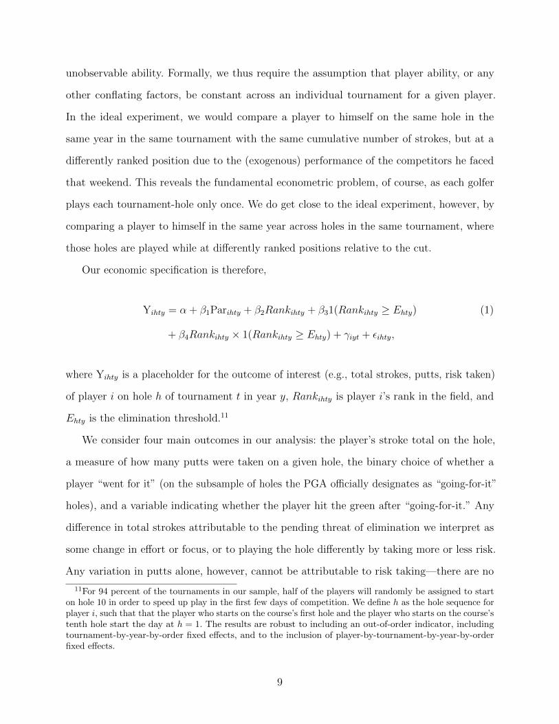
unobservable ability. Formally, we thus require the assumption that player ability, or any
other conflating factors, be constant across an individual tournament for a given player.
In the ideal experiment, we would compare a player to himself on the same hole in the
same year in the same tournament with the same cumulative number of strokes, but at a
differently ranked position due to the (exogenous) performance of the competitors he faced
that weekend. This reveals the fundamental econometric problem, of course, as each golfer
plays each tournament-hole only once. We do get close to the ideal experiment, however, by
comparing a player to himself in the same year across holes in the same tournament, where
those holes are played while at differently ranked positions relative to the cut.
Our economic specification is therefore,
Yihty = α + β1Parihty + β2Rankihty + β31(Rankihty ≥ Ehty) (1)
+ β4Rankihty × 1(Rankihty ≥ Ehty) + γiyt + εihty,
where Yihty is a placeholder for the outcome of interest (e.g., total strokes, putts, risk taken)
of player i on hole h of tournament t in year y, Rankihty is player i’s rank in the field, and
Ehty is the elimination threshold.11
We consider four main outcomes in our analysis: the player’s stroke total on the hole,
a measure of how many putts were taken on a given hole, the binary choice of whether a
player “went for it” (on the subsample of holes the PGA officially designates as “going-for-it”
holes), and a variable indicating whether the player hit the green after “going-for-it.” Any
difference in total strokes attributable to the pending threat of elimination we interpret as
some change in effort or focus, or to playing the hole differently by taking more or less risk.
Any variation in putts alone, however, cannot be attributable to risk taking—there are no
11For 94 percent of the tournaments in our sample, half of the players will randomly be assigned to starton hole 10 in order to speed up play in the first few days of competition. We define h as the hole sequence forplayer i, such that that the player who starts on the course’s first hole and the player who starts on the course’stenth hole start the day at h = 1. The results are robust to including an out-of-order indicator, includingtournament-by-year-by-order fixed effects, and to the inclusion of player-by-tournament-by-year-by-orderfixed effects.
9

options for taking risky putts, per se—which will help in identifying whether movement in
total strokes is entirely attributable to risk. (It will not be.) With respect to the return to risk
taking itself, we will interpret the player hitting the green after taking the risk as a measure
of success.
Although the actual cut occurs at the end of the second day of competition, we observe
each player’s performance on each hole of the tournament, and can therefore recreate the
status of any pending elimination that would have been faced on approach to each hole.
Given the “ties” included in the PGA Tour’s “70 plus ties” elimination rule, Ehty is a
tournament-specific elimination threshold. The indicator variable 1(rihty > Ehty) therefore
captures anyone with a rank worse than the “70 plus ties” cut as he approaches hole h and
faces elimination without some improvement. We normalize Ehty to zero in all figures and
tables below, after accounting for ties. While elimination is according to ordinal ranking, we
will also respect cardinal relationships when predicting player performance on either side of
the elimination rule and, thus, define rihty in deviations from the stroke total that would imply
elimination (within tournament, of course, and recalculated for the entire field of players
after each hole). In the end, if rihty > 0, then rihty is equal to the number of strokes i must
pick up in order to make the cut. If rihty < 0, then |rihty| is equal to the number of strokes i
could drop before he failed to make the cut. The interaction term in the model identifies the
slope parameter on rihty for those who face elimination as of hole h. In Figure 2 we report
the distribution of rank rihty over the pooled sample of all player-holes.
Our specifications are estimated using ordinary least squares, where γiyt indicates tourna-
ment specific controls for player heterogeneity, and the estimation of εihty allows for clustering
at the level of player-by-year-by-tournamant. As the estimated coefficients are implying
changes in hole-level performance, note that a small change in hole-level performance can
amount to sizable changes in 36-hole performance over two days of competition.
10

5 Results
5.1 Baseline performance results
In Column (1) of Table 1, we report estimates of a baseline specification of hole-level
performance on either side of the discontinuity in players’ expectations of survival that is
introduced by the “70 plus ties” elimination threshold. Without including controls for player
ability, the positive slope parameter on Rank in Column (1) would be consistent with the
bias driven by better players tending to have fewer strokes on average. In Column (2), we
absorb player-specific time-invariant heterogeneity into the error structure, which has the
effect of reversing the sign of the estimated slope parameter. However, golf being the game it
is, there is reason to anticipate that player ability can vary in ways that will escape player
fixed effects. (After being cut from the 2017 Farmer’s Insurance Open, Tiger Woods offered
“Unfortunately, I didn’t get a chance to win this golf tournament ... but I have next week.”)
Thus, in columns (3) and (4) we allow for year-specific player heterogeneity and tournament-
by-year-specific player heterogeneity, respectively. To the extent players have good and bad
weekends idiosyncratically, identifying the difference in player i’s performance using variation
within a given weekend of competition, when he is in and out of facing elimination over the
course of that tournament, will be our preferred specification.12 This is further supported
by the model of Column (4) yielding the most-negative slope parameter—omitting ability
would tend to drive such estimates positive—which suggests that we are better-absorbing the
effects of unobserved player ability with the less-restrictive structure.
In our preferred specification, the estimated discontinuity in performance at the elimination
margin is therefore -0.05, suggesting that players perform relatively better (than themselves,
on the same weekend) when they face elimination, and thus have nothing to lose. As the
estimated parameters are per-hole performance measures, it is noteworthy to consider that the
12It is not uncommon for the best professional golfers to have bad weekends. For example, Jordan Spieth,the world-number-one golfer at the end of 2015, failed to make it through to the third day of competition infour of the 25 PGA Tour events he entered in 2015.
11

36-hole equivalent yields a pre-cut marginal effect of -1.785 strokes—a meaningful improvement
in performance given the margins that often make the difference between a player failing to
make the cut and playing through to the final day of competition. The percent of players
missing the cut by one stroke varies (across tournaments) from 2 to 16.5 percent, with 8.7
percent of the field of players in the average tournament missing the cut by one stroke.
We will shortly turn to consider the elasticity of risk taking with respect to potential
elimination. Before doing so, we re-estimate, in Column (5), our preferred specification but
with the number of putts as the dependent variable. As putting is not subject to any choice
of risk-related strategy, this result serves to establish our prior that risk is surely not able
to explain the entire increase in performance. The estimated discontinuity is -0.03, with the
associated 36-hole equivalent of this marginal effect of -1.039. Increased performance on putts
thus explains 58 percent of the improvement in overall score, which supports that players
do indeed perform better when on the elimination side of the upcoming cut in ways that
are independent of their risk taking. Without an available appeal to risk taking to explain
this increase in performance, this improvement in score is most likely explained by increased
focus and determination when the threat of elimination is more salient.
5.2 Baseline risk-taking results
In Table 2, we adopt our preferred specification above but restrict the sample to those
holes designated by the PGA as “going-for-it” holes.13 In this table, we attempt to explain the
variation in three risk-related outcomes: whether a player went for the green on a risk-taking
hole, whether a player hit the green after taking a risk, and the distance to the hole after
taking a risky shot.14 The sample size varies across columns of Table 2 as the risk-success
outcomes are conditional on having taken the risk.
13See Table A1 for the progression of specifications leading to our preferred, as in Table 1.14If we repeat the preferred specification of strokes, but restrict the sample to those holes designated by
the PGA as “going-for-it” holes, we find similar point estimates even though there are no par-3 holes inthis sub-sample, since it is expected that all golfers will always attempt to hit the green from the tee. Thisexplains part of the decline in sample size going from Table 1 to Table 2.
12

In general, our results in Column (1) suggest that there is a positive relationship between
player rank and risk taking—a one-stroke decline in performance (an increase in rank Rank)
is associated with a roughly 1-percent increase in the propensity to take a risk, all else equal.
However, those on the elimination side of the cut choose the risky strategy 2.7 percentage
points more often, or a 5.4-percent increase in the probability of taking a risk when possible.
Given an average of 7.2 holes (out of 36) on which it is possible to take this type of risk, this
represents a potential improvement in performance of 0.19 strokes over the first two days of
competition (i.e., 7.2×.027). Thus, at the upper bound where all risk pays off, risk taking
can explain 49 percent of the gains in measured performance on “going-for-it” holes.15
In Column (2) we consider the ex post realization of risk taking. Where players take risky
strategies, the PGA records “success” quite simply as hitting the green, which we capture
with a binary outcome. Conditional on the risky strategy having been chosen, we find a
one percentage-point increase in the probability of a successful outcome on the elimination
side. Risk taking therefore explains 23 percent of the gains in measured performance on
“going-for-it” holes.16 This is consistent with relatively fruitful risk taking on the elimination
side, on average. We cannot separately identify the types of risk taken under threat of
elimination from their success rates, but this suggests that we are identifying the effect of
additional focus being brought to bear when a player faces the threat of elimination, and not
merely that they are induced into taking riskier risky shots (which would decrease rates of
success, all else equal).17
As one last attempt to capture variation in player performance around risk taking, in
Column (3) of Table 2 we consider the remaining distance to the hole after having taken a
risky shot. While the PGA records failing to hit the green after choosing the risky strategy
15Restricting Table 1 Column (4) to a sample of “going-for-it” holes yields a point estimate discontinuityof -.055. Thus, where all additional risks taken reward the player with a one-stroke improvement, the fractionof gains attributable to additional risk taking is .027/.055=.49.
16Restricting Table 1 Column (4) to a sample of “going-for-it” holes on which risk was actually taken yieldsan estimated discontinuity of -.053. Thus, accounting for rates of success, the fraction of gains attributable toadditional risk taking is .012/.053=.23.
17Re-estimating the model while including controls for the distance to the hole before the shot was takenleaves our results unchanged.
13

as failure, any systematic variation in the remaining distance to the hole may similarly point
to improved performance. Conditional on the distance their risky shot is taken from, we find
that when players face elimination they land their risky shots 13-inches closer to the hole, on
average, than when they do not face elimination. Again, we interpret the data as suggestive
that the threat of elimination is increasing “productive” risk taking.
5.3 Sensitivity, heterogeneity, and bandwidth considerations
In the analysis above we identify the average effect of a pending threat of elimination.
Below, we wish to consider whether the elasticity of performance and risk taking is evidently
different as the threat of elimination becomes more salient, and the potential sensitivity of
our results to the selection of players who contribute to identification. As it turns out, these
are all “bandwidth” considerations, in a away, so we group them together below.
5.3.1 Does responsiveness change as elimination approaches?
First, we will explore the effect of pending elimination on outcomes as the opportunities to
influence outcomes slip away—as there are few holes remaining and the threat of elimination
becomes more salient. We accomplish this by re-estimating our models while sequentially
dropping the earliest holes played in each tournament. This is also a bandwidth sensitivity of
a sort, in the sense that one might think of the cleanest identifying variation existing at the
actual elimination—the top 70 as of the end of the 36th hole continuing.
In Figure 3, for each of our four outcome variables, we report the estimated effects of
being on the elimination side of the elimination threshold across this metric. Moving to the
right on the figure, then, we restrict the sample to fewer holes—those holes closer to the
actual tournament cut at the end of the 36th hole.18 In Panel A, the estimated discontinuity
in strokes is negative throughout most of the specifications, though attenuates as we discard
18Since we are using player-by-tournament-by-year fixed effects, the last hole we can actually discard fromour sample is hole 34. Recall also that hole 1 is not identified since players are not ranked prior to posting astroke total.
14

early holes from the model, and actually flips sign as we identify only off of the threat of
elimination over the last few holes, where it is most salient. That is, on holes 35 and 36,
players are performing worse when on the elimination side of the cut. (Recall that it is
reductions in score that equate with improvements in performance.) This would be consistent
with players losing focus as the opportunities for success slip away, or simply evidence players
having limited capacity to maintain performance levels with the stress of elimination being
felt so strongly. However, as the estimated discontinuity in putts, in Panel B, is invariant
across the same sequence of specifications, we are inclined to attribute the inversion in effect
to changes in the risk adopted by players as elimination approaches—either risk taking, per
se, or the success rate of risks taken.
In Panel C we plot the estimated discontinuities for risk taking which, like putts, also
proves very stable throughout the 36 holes. With one last consideration, then, it is in Panel
D that we see the mechanism revealed—indeed, the differential conditional probability that
the player hits the green on risky shots declines as elimination approaches.
Overall, then, a consistent story would be that the performance improvements associated
with potential elimination—recall that they are in part due to successful risk taking—vanish
as elimination ultimately approaches, and that this is more attributable to decreases in
the success rate of any risks taken (Panel D) than to more or less risk being taken (Panel
C) toward the end of day two, and, as suggest by the stability of putts, also less about
risk-independent performance being any more or less responsive as elimination approaches
(Panel B).
5.3.2 Is responsiveness different for players closer to the cut on average?
In further considering the sensitivity of player responsiveness to elimination, here system-
atically remove players (not holes) from the sample. Players are amassed around the cutoff
for the first few holes, of course, and the contributions of those player-holes introduced to the
identifying variation by those who will quickly separate from the field (in either direction)
15

may not be the ideal experimental variation off of which to identify.19 For example, even
after controlling for player ability, even the tournament’s eventual winner could have easily
played the first hole at one or two strokes over par, and would thus contribute one or two
observations to the identifying variation, in ways that have little to do with any responsiveness
to pending elimination. (Such would yield negative bias, as he subsequently performed better
on the elimination side, which is what led him to eventual victory.) Clearly, the strongest
and weakest players in the field, who will necessarily contribute at least a few observations
around the cutoff, are hardly the marginal observations off of which we should identify. We
would prefer, in the sense of the ideal experiment, to find these players randomly on each side
of the elimination threshold, which we might best approximate by considering the sensitivity
of the point estimate to collapsing on those players who are closer to the cutoff on average
and are therefore most likely to experience the quasi-random play from both side of the cut.
In Figure 4 we plot the histogram of players’ average within-tournament ranks, revealing
how different players can be in their average deviation from the threshold. The truly marginal
players are arguably those clustered around the cut (at zero). In Table 3 we therefore report
estimates of the discontinuity as we remove players with average (tournament-specific) ranks
farthest away from the threshold—roughly, then, it is both the best and worst players being
eliminated as we tighten up the estimation around the discontinuity. We consider the entire
sample in the first column, those within 20 strokes of the cut in the second column, through
to using only those with a mean rank within 1 stroke of the cut. Total strokes and estimates
of putting responsiveness are very stable as the bandwidth collapses in this way, restricting
observations to players who are truly middling in each tournament.
5.3.3 Is responsiveness different for players who are around the cut more often?
As one last alternative, rather than removing players based on their average rank over the
tournament, we can collapse on players who are close to elimination most often. In Figure 5
19On average, 61 percent of the field is on the margin of being cut at hole 2.
16

we report the estimated discontinuities across increasingly restricted samples. The x-axis of
the figure represents the minimum number of times contributing players crossed the threshold
in either direction during the first 36 holes of competition. As we move to the right—this has
the sample increasingly consist of players who crossed the threshold more frequently—the
estimated discontinuity more than doubles, though loses precision in the expected way. This
suggests that, if anything, players most often at the margin of elimination are more sensitive
to which side of the threshold they are on.
5.3.4 Why not disaggregated player-rank sample restrictions?
Another possible bandwidth sensitivity exercise would increasingly restrict the sample to
tournament-year-player-holes where player ranks were nearest the cut. Given the importance
of capturing unobserved player heterogeneity, in our preferred specifications we identify only
off of within-player variation. As such, restricting the sample to only those player-holes where
the player was close to elimination (not just close on average) quickly decreases our ability
to detect any behavior of interest. More fundamentally, though, we do not perform this
exercise as the objective in collapsing around the identifying threshold is to increase the
comparability of the “treatment” and “control” groups, which this does not accomplish. For
example, a Rank-based bandwidth restriction gives increasing weight to players who will
only pass through the treatment margin in the first few holes of the tournament, before they
separate to either the front or back of the field of competitors. These players are in no way
representative of the sort of marginal player off of which we wish to identify.
5.4 Additional heterogeneity
5.4.1 Time of day
We continue with our consideration of heterogeneity in other dimensions by first including
an analysis of what could constitute a threat to identification. Though likely to impart only
attenuation bias, the time-staggered play across the field of competitors may matter insofar
17

as early groups are less informed about the stroke totals that will contribute to the “70 plus
ties” elimination threshold (i.e., the Ehty above).
To partially address this, we stratify the model by the hour each hole was finished. To
avoid conflating the time of day and hole sequence, we control for hole sequence directly. In
Figure 6 we report the estimated discontinuities, noting again that the confidence interval
natural widens around observations at the end of the day, where there are fewer observations.
In the end, however, we find the estimates quite robust to time of play. Even though morning
players are arguably less informed than afternoon afternoon players, those in the morning
are not seeming to react to potential elimination any less than those in the afternoon.
This is consistent with professionals knowing about where the cut line is going to be
and reacting to that expectation. In Figure 7 we present a histogram of the relative-to-
par elimination threshold across tournaments. In short, this suggests that the threshold is
predictable, with a reasonably significant ability to do so even before the tournament has
begun. Thus, it isn’t surprising that disparities in information don’t seem to change the point
estimates, especially considering that players will include knowledge of course and tournament
heterogeneity.
5.4.2 Field- and player-specific ability
We next explore heterogeneous responses to the threshold. As players select into tourna-
ments, it is interesting to consider heterogeneity by tournament, which we do by separately
considering tournaments for which at least 30 percent, 50 percent, and 70 percent of the field
is world ranked (according to the OWGR), respectively. Estimated discontinuities across these
very different average-ability levels reveal no differential responsiveness to finding oneself on
the elimination side of the cut, enough so that we are inclined to believe that differential
selection into tournaments is not contributing to our results. These estimates are reported in
Table 4.
We also consider heterogeneity at the player level. In Table 5 we stratify the sample into
18

ranked and unranked players, and then separately estimate the discontinuity for unranked
players, and then for stronger and stronger pools of ranked players. Doing so reveals that
higher-ranking players respond less at the margin to potential elimination. The estimated
discontinuity on stroke totals for the highly ranked players is about half the size as it is for
the unranked players and the estimated discontinuity on putts is also smaller.
Moreover, the risk-taking behavior and subsequent risk success of highly ranked players
does not differ with pending elimination. This pattern is consistent with differences in
experience—more-experienced players know better or are more comfortable with their style
of play, thus being less sensitive to conditions. Essentially, a sign of maturity and expertise
may well yield lower elasticities with respect to pending elimination.
It is also the case that as we collapse on higher-ranking players, we are collapsing on
players who are increasingly likely to make a given cut, and thereby secure prize winnings
with greater likelihood and in larger amount.
Among the highly ranked, the performance increase in strokes due to the pending elimi-
nation is similar in magnitude to the performance increase in putts, implying that increased
putting concentration and focus can completely explain the overall performance increase.
5.4.3 Hole difficulty
Opportunities to gain strokes vary according to the hole’s par, necessitating the use of par
as a control variable in our preferred specification. It is somewhat natural to then consider
the potential heterogeneity across par. In Table 7 we report changes in our outcome variables
across par-3, par-4, and par-5 holes separately.20
The estimated discontinuity in all four outcomes is somewhat larger in magnitude as
the par of the hole increases. That is, players are more likely to gain strokes in response to
elimination on the longer par-5 holes, where there are more opportunities to gain strokes.21
20As no par-3 holes are ever classified as “going-for-it” holes, the two risk-dependent variables cannot beestimated on par-3 holes.
21This is backed up by the data, with 8,559 instances of players scoring an eagle on par-5 holes and only212 instances of the same feat on par-3 holes.
19

However, we see evidence of performance responding in similar ways even on the shorter par-3
holes, which again reflects that risk taking is not fully accounting for changes in performance.22
Players are also more risk-responsive to pending elimination on par-5 holes than on par-4
holes. Concerning returns to risk, when on the elimination side of the cut players are also
more likely to hit the green after taking a risk on par-5 holes.23
5.4.4 Does a player’s history of elimination matter?
In Table 6 we stratify by whether a player’s most-recent experience on the ended with
him being eliminated after 36 holes, or not. Doing so suggests that those who were eliminated
in their most-recent tournament were, if anything, less responsive to playing under pending
elimination. As we have absorbed player-specific fixed effects into the error structure of our
preferred specification, this implies that those coming of an elimination play more similarly
on either side of the pending cut than do those who successfully made it to the third day of
competition in their most-recent tournament. This slight increase in responsiveness to the
threat among those with recent success holds across total strokes, putts, risk taking, and in
the probability that risk end in success. While we have no strong priors, this is consistent with
heightened expectations from recent success interacting with the current threat of elimination
to produce more of a motivating device.
6 Conclusion
The PGA records enable hole-by-player-by-tournament analysis around objectively deter-
mined cutoffs, where players are routinely observed around either side of the threshold of
elimination-style tournaments. We can approximate the ideal experiment by comparing a
player to himself across holes in the first two days of a single tournament. On some holes, he
22Recall that there are not risks to take on par-3 holes.23This can’t be explained by differences in hole difficulty as more players succeed in hitting the green on
par-4 holes than par-5 holes. Across all players, there is a 23-percent risk-success rate for par-5 holes and25-percent risk-success rate for par-4 holes.
20

will be on the elimination side of the threshold, while on other holes he will be on the safe
side.
We exploit an opportunity to jointly observe performance, ex ante risk taking, and the
ex post realization of risk. Collectively, we paint a picture of performance, risk taking, and
rates of success on risks taken, each being higher when players play from the elimination
side of the elimination threshold. Our results are robust to a battery of sensitivity exercises,
and strongly suggest that sensitivity to elimination is stronger in lower-ability players. In
particular, while measured performance does improves, there is no evident increase in risk
taking among those of highest ability.
21

References
Barron, John M. and Glen R. Waddell, “Work Hard, Not Smart: Stock Options inExecutive Compensation,” Journal of Economic Behavior & Organization Organization,2008, 66, 767–790.
Becker, Brian E and Mark A Huselid, “The Incentive Effects of Tournament Compen-sation Systems,” Administrative Science Quarterly, 1992, pp. 336–350.
Bothner, Matthew S., Jeong han Kang, and Toby E. Stuart, “Competitive Crowdingand Risk Taking in a Tournament: Evidence from NASCAR Racing,” Administrative ScienceQuarterly, 2007, 52 (2), 208–247.
Brown, Jennifer, “Quitters Never Win: The (Adverse) Incentive Effects of Competing withSuperstars,” Journal of Political Economy, 2011, 119 (5), 982–1013.
Cabral, Luis, “R&D Competition When Firms Choose Variance,” Journal of Economics &Management Strategy, 2003, 12 (1), 139–150.
Chevalier, Judith and Glenn Ellison, “Risk Taking by Mutual Funds as a Response toIncentives,” Journal of Political Economy, 1997, 105 (6), 1167–1200.
Ehrenberg, Ronald G. and Michael L. Bognanno, “Do Tournaments Have IncentiveEffects?,” Journal of Political Economy, 1990, 98 (6), 1307–1324.
and , “The Incentive Effects of Tournaments Revisited: Evidence from the EuropeanPGA Tour,” Industrial and Labor Relations Review, 1990, 43 (3), 74S–88S.
Garcia, Jose M. and E. Frank Stephenson, “Does Stableford Scoring Incentivize MoreAggressive Golf?,” Journal of Sports Economics, 2015, 16 (6), 647 – 663.
Genakos, Christos and Mario Pagliero, “Interim Rank, Risk Taking, and Performancein Dynamic Tournaments,” Journal of Political Economy, 2012, 120 (4), 782–813.
Grund, Christian, Jan Hocker, and Stefan Zimmermann, “Incidence and Conse-quences of Risk-Taking Behavior in Tournaments–Evidence from the NBA,” EconomicInquiry, 2013, 51 (2), 1489 – 1501.
Guryan, Jonathan, Kory Kroft, and Matthew J Notowidigdo, “Peer Effects in theWorkplace: Evidence from Random Groupings in Professional Golf Tournaments,” AmericanEconomic Journal: Applied Economics, 2009, 1 (4), 34–68.
Imas, Alex, “The Realization Effect: Risk-Taking After Realized Versus Paper Losses,” TheAmerican Economic Review, 2016, 106 (8), 2086–2109.
Knoeber, Charles R. and Walter N. Thurman, “Testing the Theory of Tournaments:An Empirical Analysis of Broiler Production,” Journal of Labor Economics, 1994, 12 (2),155–179.
22

Lazear, Edward P. and Sherwin Rosen, “Rank-Order Tournaments as Optimum LaborContracts,” Journal of Political Economy, 1981, 89 (5), 841–864.
McFall, Todd and Kurt W Rotthoff, “Risk Taking Dynamics in Tournaments: Evidencefrom Professional Golf,” Working Paper, 2016.
Mueller-Langer, Frank and Patrick Andreoli Versbach, “Leading-effect vs. Risk-taking in Dynamic Tournaments: Evidence from a Real-life Randomized Experiment,”Munich Discussion Paper No. 2013-6, 2013.
Orszag, Jonathan M., “A New Look at Incentive Effects and Golf Tournaments,” Eco-nomics Letters, 1994, 46 (1), 77 – 88.
Ozbeklik, Serkan and Janet Kiholm Smith, “Risk Taking in Competition: Evidencefrom Match Play Golf Tournaments,” Journal of Corporate Finance, 2014, pp. –.
Pope, Devin G and Maurice E Schweitzer, “Is Tiger Woods Loss Averse? PersistentBias in the Face of Experience, Competition, and High Stakes,” The American EconomicReview, 2011, 101 (1), 129–157.
Prendergast, Canice, “The Provision of Incentives in Firms,” Journal of Economic Litera-ture, 1999, 37 (1), 7–63.
Taylor, Beck A and Justin G Trogdon, “Losing to Win: Tournament incentives in theNational Basketball Association,” Journal of Labor Economics, 2002, 20 (1), 23–41.
Taylor, Jonathan, “Risk-Taking Behavior in Mutual Fund Tournaments,” Journal ofEconomic Behavior & Organization, 2003, 50 (3), 373 – 383.
23

Figures
Figure 1: How many players make the “70 plus ties” cut
Notes: Given ties, the number of players who make the cut after 36 holes of play can exceed 70. In
this figure, we plot the histogram of the number of players who make the cut in a given tournament,
across all stroke-play tournaments on the PGA Tour, 2002-2016.
24

Figure 2: Deviations from tournament cut (Rank)
Notes: Given deviations from the implicit elimination threshold on each hole of play on the PGA
Tour (Ehty), we plot the histogram of player rank at each hole (measured in strokes) relative to the
elimination threshold, across all stroke-play tournaments on the PGA Tour, 2002-2016.
25

Figure 3: Does responsiveness change as elimination approaches?
Panel A: Total strokes Panel B: Putts
Panel C: 1(Went for it) Panel D: 1(Hit the green)
Notes: Point estimates and 95-percent confidence intervals from repeated estimations of Equation
(1), restricting the sample to holes successively closer to elimination.
26

Figure 4: Mean rank of players
Notes: Given deviations from the implicit elimination threshold on each hole, we plot the histogram
of average player rank (measured in strokes) relative to the elimination threshold, across all
stroke-play tournaments on the PGA Tour, 2002-2016.
27

Figure 5: The estimated discontinuity by number of threshold crossings
Panel A: Total strokes Panel B: Putts
Panel C: 1(Went for it) Panel D: 1(Hit the green)
Notes: Point estimates and 95-percent confidence intervals from repeated estimations of Equation
(1), restricting the sample to those “closer” to elimination, defined as having more crossings of the
elimination threshold.
28

Figure 6: Heterogeneity by hour of play
Panel A: Total strokes Panel B: Putts
Panel C: 1(Went for it) Panel D: 1(Hit the green)
Notes: Point estimates and 95-percent confidence intervals from repeated estimations of Equation
(1), stratified by the (player-specific) hour play was completed.
29

Figure 7: How predictable is the elimination threshold?
Notes: In this figure we plot the histogram of strokes relative to par that constituted the “70 plus
ties” cut across all stroke-play tournaments on the PGA Tour, 2002-2016.
30

Tables
31

Table 1: The performance gains under pending elimination
Strokes per holePutts
only
(1) (2) (3) (4) (5)
1(Rank ≥ 70) -0.012*** 0.002 0.006*** -0.050*** -0.029***
(0.001) (0.001) (0.001) (0.002) (0.001)
Rank 0.0002 -0.002*** -0.004*** -0.063*** -.031***
(0.0003) (0.0003) (0.0003) (0.0004) (0.0003)
Rank × 1(Rank ≥ 70) 0.0154*** 0.006*** 0.002*** 0.013*** 0.0097***
(0.0005) (0.0005) (0.0005) (0.0007) (0.0005)
Par 0.827*** 0.827*** 0.826*** 0.816*** -0.035***
(0.0007) (0.0007) (0.0007) (0.0007) (0.0006)
Constant 0.685*** 1.263*** 0.625*** 0.754*** 1.742***
(0.003) (0.075) (0.003) (0.003) (0.002)
Observations 2,519,650 2,519,650 2,519,650 2,519,650 2,519,650
R2 0.377 0.382 0.385 0.405 0.010
Player FE No Yes No No No
Player-by-year FE No No Yes No No
Player-by-year-by-tournament FE No No No Yes Yes
Mean (depvar) 3.96 3.96 3.96 3.96 1.60
Number of groups 2,555 8,637 71,990 71,990
Implied change in strokes (per t) -1.785 -1.039
Notes: Standard errors in parentheses, allowing for clustering at the player-by-year-by-tournamentlevel. *** p<0.01, ** p<0.05, * p<0.1
32

Table 2: Risk taking under pending elimination
1(Went for it) = 1
1(Went for it) 1(Hit green)Distance
remaining
(1)a (2)a (3)
1(Rank ≥ 70) 0.027*** 0.012*** -13.372***
(0.003) (0.003) (3.340)
Rank 0.011*** 0.009*** -5.557***
(0.0006) (0.0008) (0.727)
Rank × 1(Rank ≥ 70) 0.003*** -0.003** 1.974*
(0.0009) (0.001) (1.106)
Par 0.037*** 0.130*** -146.008***
(0.002) (0.002) (4.648)
Constant 0.305*** -0.379*** 699.407***
(0.012) (0.012) (31.60)
Observations 445,158 221,865 221,865
R2 0.005 0.016 0.122
Mean (depvar) 0.498 0.242 673.323
Number of groups 63,423 58,613 58,613
Notes: All specifications absorb player-by-year-by-tournament unobserved het-erogeneity into the error structure. Standard errors in parentheses, allowing forclustering at the player-by-year-by-tournament level. *** p<0.01, ** p<0.05, *p<0.1. a Linear-probability models, though binary response models yield qualita-tively similar results.
33

Table 3: Bandwidth sensitivity by mean rank of player
Absolute deviation (in strokes) from
elimination threshold
|µr| ≤ 20 |µr| ≤ 10 |µr| ≤ 5 |µr| ≤ 1
(1) (2) (3) (4)
Panel A: Strokes
1(Rank ≥ 70) -0.050*** -0.048*** -0.039*** -0.050***
(0.002) (0.002) (0.002) (0.003)
Observations 2,519,650 2,516,885 2,352,525 715,680
Panel B: Putts
1(Rank ≥ 70) -0.029*** -0.028*** -0.023*** -0.020***
(0.001) (0.001) (0.001) (0.002)
Observations 2,519,650 2,516,885 2,352,525 715,680
Panel C: 1(Went for it)
1(Rank ≥ 70) 0.027*** 0.026*** 0.021*** 0.021***
(0.003) (0.003) (0.003) (0.005)
Observations 445,158 444,684 415,562 126,400
Panel D: 1(Hit the green) conditional on 1(Went for it)=1
1(Rank ≥ 70) 0.012*** 0.011*** 0.010*** 0.015***
(0.003) (0.003) (0.003) (0.005)
Observations 221,865 221,671 206,636 62,382
Notes: All specifications include par, and absorb player-by-year-by-tournamentunobserved heterogeneity into the error structure. Standard errors in parentheses,allowing for clustering at the player-by-year-by-tournament level. *** p<0.01, **p<0.05, * p<0.1 34

Table 4: Heterogeneity by average ability of the field of competitors
% of field with OWGR ranking
Full sample ≥ 30 ≥ 50 ≥ 70
(1) (2) (3) (4)
Panel A: Strokes
1(Rank ≥ 70) -0.050*** -0.050*** -0.054*** -0.057***
(0.002) (0.002) (0.002) (0.003)
Observations 2,572,654 2,354,695 1,649,900 645,015
Panel B: Putts
1(Rank ≥ 70) -0.029*** -0.029*** -0.030*** -0.028***
(0.001) (0.001) (0.002) (0.003)
Observations 2,572,654 2,354,695 1,649,900 645,015
Panel C: 1(Went for it)
1(Rank ≥ 70) 0.027*** 0.029*** 0.031*** 0.031***
(0.003) (0.003) (0.003) (0.005)
Observations 445,158 419,542 301,078 127,078
Panel D: 1(Hit green) conditional on 1(Went for it)=1
1(Rank ≥ 70) 0.012*** 0.013*** 0.015*** 0.019***
(0.003) (0.003) (0.004) (0.005)
Observations 221,865 208,883 153,307 66,793
Notes: All specifications include par, and absorb player-by-year-by-tournamentunobserved heterogeneity into the error structure. Standard errors in paren-theses, allowing for clustering at the player-by-year-by-tournament level. ***p<0.01, ** p<0.05, * p<0.1
35

Table 5: Heterogeneity by player ability
Unranked OWGR-ranked players
players 1-300 1-200 1-100 1-50
(1) (2) (3) (4) (5)
Panel A: Strokes
1(Rank ≥ 70) -0.051*** -0.036*** -0.038*** -0.030*** -0.021***
(0.002) (0.002) (0.003) (0.004) (0.005)
Observations 1,096,270 1,423,380 1,183,455 635,495 325,220
Panel B: Putts
1(Rank ≥ 70) -0.032*** -0.020*** -0.021*** -0.020*** -0.021***
(0.002) (0.002) (0.002) (0.003) (0.004)
Observations 1,096,270 1,423,380 1,183,455 635,495 325,220
Panel C: 1(Went for it)
1(Rank ≥ 70) 0.029*** 0.022*** 0.020*** 0.006 0.006
(0.004) (0.004) (0.004) (0.005) (0.008)
Observations 188,045 257,113 214,492 116,356 59,776
Panel D: 1(Hit green) conditional on 1(Went for it)=1
1(Rank ≥ 70) 0.009* 0.009** 0.007 0.009 0.012
(0.005) (0.004) (0.005) (0.006) (0.008)
Observations 89,001 132,864 112,793 64,634 34,574
Notes: All specifications include par, and absorb player-by-year-by-tournament unob-served heterogeneity into the error structure. Standard errors in parentheses, allowingfor clustering at the player-by-year-by-tournament level. *** p<0.01, ** p<0.05, * p<0.1
36

Table 6: Heterogeneity by cut outcome of most-recent tournament
Outcome in most-recent
tournament
EliminatedNot
eliminated
(1) (2)
Panel A: Strokes
1(Rank ≥ 70) -0.036*** -0.048***
(0.002) (0.002)
Observations 1,406,195 1,031,415
Panel B: Putts
1(Rank ≥ 70) -0.024*** -0.026***
(0.002) (0.002)
Observations 1,406,195 1,031,415
Panel C: 1(Went for it)
1(Rank ≥ 70) 0.023*** 0.027***
(0.004) (0.004)
Observations 251,455 179,957
Panel D: 1(Hit green) conditional on 1(Went for it)=1
1(Rank ≥ 70) 0.009** 0.011**
(0.004) (0.005)
Observations 127,377 86,759
Notes: All specifications include par, and absorb player-by-year-by-tournament unobserved heterogeneity into the error structure. Firsttournament for all players discarded. Standard errors in parentheses,allowing for clustering at the player-by-year-by-tournament level.*** p<0.01, ** p<0.05, * p<0.1
37

Table 7: Heterogeneity by par of hole
Par 3 Par 4 Par 5
(1) (2) (3)
Panel A: Strokes
1(Rank ≥ 70) -0.036*** -0.047*** -0.056***
(0.003) (0.002) (0.004)
Observations 578,327 1,496,835 444,470
Panel B: Putts
1(Rank ≥ 70) -0.020*** -0.029*** -0.031***
(0.003) (0.002) (0.003)
Observations 578,327 1,496,835 444,470
Panel C: 1(Went for it)
1(Rank ≥ 70) 0.014*** 0.026***
(0.004) (0.003)
Observations 86,117 359,041
Panel D: 1(Hit green) conditional on 1(Went for it)=1
1(Rank ≥ 70) 0.0001 0.014***
(0.003) (0.004)
Observations 51,592 170,273
Notes: All specifications absorb player-by-year-by-tournament unobservedheterogeneity into the error structure. Standard errors in parentheses,allowing for clustering at the player-by-year-by-tournament level. ***p<0.01, ** p<0.05, * p<0.1
38

7 Appendix
39

Table A1: “Baseline” specifications for other outcomes
(1) (2) (3) (4)
Panel A: Putts
Rank -0.0002 0.0006 0.0003 -0.031***
(0.0003) (0.0005) (0.0004) (0.0003)
1(Rank ≥ 70) -0.006*** -0.003* -0.001 -0.029***
(0.001) (0.002) (0.002) (0.001)
r × 1(Rank ≥ 70) 0.002*** -0.0009 -0.001** 0.010***
(0.0004) (0.0006) (0.0006) (0.0005)
Observations 2,572,654 2,572,654 2,572,654 2,572,654
Panel B: 1(Went for it)
Rank -0.0008* 0.0008 0.001* 0.011***
(0.0005) (0.0009) (0.0008) (0.0006)
1(Rank ≥ 70) 0.023*** 0.020*** 0.022*** 0.027***
(0.002) (0.003) (0.002) (0.002)
r × 1(Rank ≥ 70) 0.0003 0.002 0.003*** 0.003***
(0.0007) (0.001) (0.001) (0.0008)
Observations 466,344 466,344 466,344 466,344
Panel C: 1(Hit green) conditional on 1(Went for it)=1
Rank 0.008*** 0.006*** 0.003*** 0.009***
(0.0006) (0.001) (0.0007) (0.0007)
1(Rank ≥ 70) -0.006** -0.004 0.001 0.011***
(0.003) (0.004) (0.003) (0.003)
r × 1(Rank ≥ 70) -0.009*** -0.008*** -0.004*** -0.003***
(0.0008) (0.002) (0.001) (0.001)
Observations 235,770 235,770 235,770 235,770
Player FE No Yes No No
Player-by-year FE No No Yes No
Player-by-year-by-tournament FE No No No Yes
Notes: All specifications include par, and absorb player-by-year-by-tournament unob-served heterogeneity into the error structure. Standard errors in parentheses, allowingfor clustering at the player-by-year-by-tournament level. *** p<0.01, ** p<0.05, *p<0.1 40