DISULFIDE BOND DETERMINATION BY COMBINING

EFFICIENT SEARCH AND MACHINE LEARNING

A thesis submitted to the faculty of

San Francisco State University

In partial fulfillment of

The Requirements for

The Degree

Master of Science

In

Computer Science: Computing for Life Sciences

by

William Henrique Elias Murad

San Francisco State University

December, 2010

Copyright by

William Henrique Elias Murad

2010

CERTIFICATION OF APPROVAL

I certify that I have read Disulfide Bond Determination by Combining Efficient Search

and Machine Learning by William Henrique Elias Murad, and that in my opinion this

work meets the criteria for approving a thesis submitted in partial fulfillment of the

requirements for the degree: Master of Science in Computer Science: Computing for Life

Sciences at San Francisco State University.

_________________________________

Rahul Singh

Professor of Bioinformatics

_________________________________

Hui Yang

Professor of Data Mining

_________________________________

Robert Yen

Professor of Biochemistry

DISULFIDE BOND DETERMINATION BY COMBINING

EFFICIENT SEARCH AND MACHINE LEARNING

William Henrique Elias Murad

San Francisco, California

2010

Background

Determining the disulfide (S-S) bond pattern in a protein is often crucial for

understanding its structure and function. In recent research, mass spectrometry (MS)

based analysis has been applied to this problem following protein digestion under both

partial reduction and non-reduction conditions. However, this paradigm still awaits

solutions to certain algorithmic problems fundamental amongst which is the efficient

matching of an exponentially growing set of putative S-S bonded structural alternatives to

the large amounts of experimental spectrometric data. Current methods circumvent this

challenge primarily through simplifications, such as by assuming only the occurrence of

certain ion-types (b-ions and y-ions) that predominate in the more popular dissociation

methods, such as collision-induced dissociation (CID). Unfortunately, this can adversely

impact the quality of results.

Method

This work presents an algorithmic approach to this problem that can, with high

computational efficiency, analyze multiple ions types (a, b, bo, b*, c, x, y, yo, y*, and z)

and deal with complex bonding topologies. The proposed approach combines (1) an

approximation algorithm-based search formulation with data driven parameter estimation

and (2) machine learning techniques which are used to train a SVM classifier, based on

previously annotated data from the Swiss-Prot knowledgebase. This proposed

formulation considers only those regions of the search space where the correct solution

resides with a high likelihood. Putative disulfide bonds thus obtained are finally

combined in a globally consistent pattern to yield the overall disulfide bonding topology

of the molecule. Additionally, each bond is associated with either a confidence score

(MS-based bonds) or a similarity score (SVM-based bonds), which aid in interpretation

and assimilation of the results.

Results

The method was tested on nine different eukaryotic Glycosyltransferases possessing

disulfide bonding topologies of varying complexity. Its performance was found to be

characterized by high efficiency (in terms of time and the fraction of search space

considered), sensitivity, specificity, and accuracy. An implementation of the method is

available at: http://tintin.sfsu.edu/~whemurad/disulfidebond.

Conclusions

This work addresses some of the significant challenges in MS-based disulfide bond

determination. This is the first algorithmic work that can consider multiple ion types in

this problem setting while simultaneously ensuring polynomial time complexity and high

accuracy of results. It is also the first solution to combine MS-based methods with

machine learning to determine the disulfide linkage of proteins. In this scenario, machine

learning techniques are used to circumvent some of the limitations of MS-based methods.

The analysis of the results shows that the blend of both state-of-the-art strategies allowed

the implementation of a solution which performed as well or better than the competing

techniques.

I certify that the Abstract is a correct representation of the content of this thesis.

_______________________________________________ ______________

Rahul Singh, Chair, Thesis Committee Date

vii

TABLE OF CONTENTS

Abstract .............................................................................................................................. iv

List of Tables ..................................................................................................................... ix

List of Figures ..................................................................................................................... x

List of Appendices ............................................................................................................. xi

Introduction ......................................................................................................................... 1

Problem Statement .......................................................................................................... 2

Review of Prior Work ......................................................................................................... 5

Background and Formulation ........................................................................................... 11

Definitions ..................................................................................................................... 11

Illustrative Examples ..................................................................................................... 14

Mass Spectrometry ........................................................................................................ 16

Blind Spot ...................................................................................................................... 24

Method .............................................................................................................................. 25

The subset-sum formulation: Towards polynomial-time matching .............................. 28

Polynomial time DMS mass list construction ............................................................... 29

Parameters Estimation ................................................................................................... 32

Polynomial time FMS construction ............................................................................... 34

Match score for S-S bonds determined using MS/MS data .......................................... 36

Integration with predictive techniques .......................................................................... 36

Support Vector Machine (SVM) ................................................................................... 38

SVM-based predictive framework ................................................................................ 40

Match score for S-S bonds determined using predictive techniques ............................ 45

Determining the globally consistent bond topology ..................................................... 46

Results ............................................................................................................................... 47

Analysis of efficiency of the search .............................................................................. 48

viii

Effects of incorporating multiple ion types: A case study ............................................ 50

Effects of integrating the predictive framework with the MS-based framework .......... 53

Comparative studies with predictive techniques ........................................................... 53

Comparative studies with MassMatrix .......................................................................... 54

Quantitative assessment and analysis of the method’s performance ............................ 56

Software ............................................................................................................................ 58

Implementation.............................................................................................................. 58

Usage Example .............................................................................................................. 61

Conclusions ....................................................................................................................... 62

References ......................................................................................................................... 63

Appendix A ....................................................................................................................... 73

Action of APPROX-DMS on the protein Beta-LG ....................................................... 73

Appendix B ....................................................................................................................... 74

Etudes of the proof of polynomial complexity .............................................................. 74

Appendix C ....................................................................................................................... 75

Combination between b/y ions and other ions types on MS/MS data .......................... 75

ix

LIST OF TABLES

Table Page

1. Abbreviations and their definitions ..............................................................................13

2. Running APROX-DMS on the ST8SiaIV C142-C292 bond ...........................................31

3. DMS and FMS mass space sizes comparison ..............................................................47

4. Comparison with predictive methods ..........................................................................53

5. Comparison with MassMatrix ......................................................................................54

6. Sensitivity, specificity, accuracy and Mathew’s correlation coefficient results for all nine proteins analyzed .......................................................................................................56

7. DMS, TrimSet and IM mass sets for each CCPi mass value generated from the tryptic digestion of the protein Beta-lactoglobulin (Beta-LG) ......................................................72

8. Different combinations of multiple ion types present in some of the proteins used to validate the method proposed ...........................................................................................74

x

LIST OF FIGURES

Figure Page

1. Disulfide bond formation and cysteine structure ............................................................1

2. The general structure of an amino acid .........................................................................11

3. Lysozyme polypeptide chain ........................................................................................12

4. The components of a mass spectrometry experiment ...................................................19

5. Search-and-match diagram and multiple ions representation ......................................25

6. Presence of multiple ions types after CID ...................................................................25

7. Two-stage matching spectra for protein ST8SiaIV .....................................................27

8. Pseudo code for APROX-DMS routine .......................................................................29

9. Pseudo code for APROX-FMS routine ........................................................................34

10. Disulfide bond types ....................................................................................................37

11. SVM: representation of a hyperplane dividing data points with two attributes (2-D) .39

12. Comparison of the computational time (in seconds) for the exhaustive and partial generation of DMS and FMS of the proteins from Table 3 ................................................48

13. Spectra illustrating the confirmatory matches found for the disulfide bond between cysteines C318-C321 in protein FucT VII .............................................................................50

14. MS2DB+ interface .......................................................................................................61

xi

LIST OF APPENDICES

Appendix Page

1. Action of APPROX-DMS on the protein Beta-LG .....................................................72

2. Etudes of the proof of polynomial complexity .............................................................73

3. Combination between b/y ions and other ions types on MS/MS data .........................74

1

Introduction

A disulfide bond, also called S-S bond or disulfide bridge, is a single covalent

bond formed from the oxidation of sulfhydryl groups (Figure 1). The oxidation process

that forms interchain disulfide bonds can produce stable covalently linked proteins,

whereas intrachain S-S bonds contribute to folding and stability. Disulfide bonds have

been classified into three categories: structural, catalytic or allosteric. Structural disulfide

bonds play an important role in the folding and stabilization of proteins. Catalytic bonds

mediate thiol-disulfide interchange reactions in substrate proteins and are important for

regulation of enzymatic activity. Allosteric disulfide bonds, in contrast to catalytic

disulfides, control the functioning of proteins by triggering changes in the intra-molecular

or inter-molecular protein structure, acting essentially as switches for protein function

[1].

Figure 1 – Disulfide bond formation (left) and cysteine structure (right)

Among the 20 natural amino acids, cysteine is unique because it is involved in

many biological activities through oxidation and reduction to form disulfide bonds and

sulfhydryls [2]. Disulfide bonds play an important role in understanding protein folding,

2

evolution, and structural properties, imposing length and angle constraints on the

backbone of a protein. Therefore, the identification of proteins disulfide connectivity is

crucial to understand their structure and function. However, the determination of

disulfide bonds can be a challenging task.

Early computational approaches for S-S bond determination focused on two

learning-driven formulations based on the protein primary structure [1]: residue

classification (distinguish bonded and free cysteines) and connectivity prediction

(determine the S-S connectivity pattern). In recent times, the increasing availability and

accuracy of mass spectrometry [2] (MS) has opened up an alternate approach; its essence

lies in matching the theoretical spectra of ionized peptide fragments with experimentally

obtained spectra to identify the presence of specific S-S bonds.

Problem Statement

Following the improvements in mass spectrometry, MS-based methods generally

outperform methods using sequence-based learning formulations, as showed by Lee and

Singh [3]. However, a number of algorithmic challenges remain outstanding in realizing

the potential of MS-based approaches. Salient among these are: (1) accounting for

multiple ion types in the data [4, 5]: To avoid an exponential increase in the search space,

a common simplification is to limit the analysis to the spectra of b-ions and y-ions only.

However, this simplification may erroneously ignore the occurrence of other ions, such

3

as: a, bo, b*, c, x, yo, y*, and z. (2) Design of efficient search and matching algorithms:

The search space of possible disulfide topologies increases rapidly not only with the

number of ion types being analyzed but also with the number of cysteines as well as the

types of connectivity patterns. Thus, it is imperative to have algorithms that can

accommodate the richness of the entire problem domain. (3) Automated data-driven

determination of parameters: Many advanced algorithms in this area are intrinsically

parametric. Often, determining the optimal value of these parameters automatically is in

itself, a complex problem. This places the practitioner at a significant disadvantage.

Support for automated and data-driven strategies for estimation of crucial parameters is

therefore crucial to the real-world success of a method in this problem domain. (4)

Addressing the limitation of MS-based approaches: Although MS-based approaches are

powerful methods for determining disulfide connectivity, it fails when the MS/MS

spectra contains blind spots. A blind spot occurs when the precursor ion fragmentation

produces different fragments only at the outside boundaries (A) of the intra-disulfide

bond or (B) of the inter-chain cross-linked disulfide bonds. This can cause too few

product ions to be generated; thus the limited information can prevent accurate

determination of disulfide bonds using MS-based methods.

The contributions of this work in context of the aforementioned challenges

include: (1) Development of a highly efficient strategy for multi-ion disulfide bond

analysis by considering a, b, bo, b*, c, x, y, yo, y*, and z ion types. To the best of our

4

knowledge, this is the first algorithmic work that has considered all these ion-types in S-S

bond determination. (2) A fully polynomial-time algorithm that selectively generates only

those regions of the search space where the correct solutions reside with a high

likelihood. (3) A multiple-regression-based data driven method to calculate the critical

parameters modulating the search, so as to ensure that the correct bonding topologies are

not missed due to the truncation of the search space. At the same time, the parameter

selection ensures that the search is focused on the most promising regions of the search-

space. (4) A local-to-global strategy that builds a globally consistent bonding pattern

based on MS data at the level of individual bonds. (5) Assignment of probability-based

scores [6] to each specific disulfide bond based on the number of MS/MS matches and

their respective abundance. These scores represent an assessment of quality and reflect

the significance of the disulfide bond and (6) Fusion of predictive techniques with the

MS-based method to address the limitations imposed by “spotty” MS/MS spectra. This

novel approach represents a break-through in the determination of disulfide bonds. It

combines the efficiency of MS-based methods with the autonomy of predictive

techniques, creating a method which is able to determine the disulfide connectivity of

proteins with high accuracy.

5

Review of Prior Work

In this section, different applications developed to determine proteins disulfide

connectivity based on either sequence-based connectivity prediction or mass

spectrometry data S-S bond identification are reviewed. First, it is important to note that a

disulfide linkage pattern can be represented by an undirected graph, where the set of

vertices correspond to the set of bonded cysteines and every edge corresponds to a

disulfide bond. This motivated the work from Fariselli and Casadio [7-9]. They used a

graph-based approach to determine the disulfide linkage by solving the maximum weight

matching problem. From a completely connected graph G formed by v vertices

corresponding to the v cysteines and edges with non-zero weights

corresponding to possible disulfide bonds, the disulfide connectivity was defined as the

solution of the maximum weight matching problem on G.

Another sequence-based connectivity prediction method was developed in [10].

Vullo and Frasconi used recursive neural networks (RNN) for scoring labeled undirected

graphs that represented disulfide bond connectivity patterns. RNN outperformed the work

of Fariselli and Casadio because RNN allowed the addition of evolutionary information,

incorporating multiple alignment profiles in the graphical representation of disulfide

connectivity patterns. The used of RNN led the way of the DISULFIND prediction server

[11]. DISULFIND uses a combination of machine learning algorithms to predict intra-

6

chain bridges from the protein sequence alone. It solves the prediction problem in two

steps. First, the bonding state of each cysteine is predicted by a SVM binary classifier.

Next, cysteines known to participate in the formation of S-S bonds are represented in an

undirected graph whose vertices are cysteines and the edges are disulfide bridges. The

most probable connectivity pattern is found by the use of a recursive neural network.

Ferre and Clote [12-13] used secondary structure information and diresidue

frequencies to develop their web server called DiANNA using a three-step procedure.

First, a neural network was trained to recognize cysteines in an oxidized state (sulphur

covalently bonded) as distinct from cysteines in a reduced state (sulphur occurring in

reactive sulfhydryl group SH). The neural network input is a window of size w centered

at each cysteine in the sequence. The second neural network is used to score each pair of

symmetric window from the previous step. This time, the network input contains

evolutionary information obtained by the use of PSIBLAST [14] and PSIPRED [15].

Finally, the algorithm calculates the maximum weight matching (similar to the approach

implemented by Fariselli and Casadio) of the formed undirected graph (output from the

second neural network) to infer the most probable disulfide bond connectivity.

Zhao et al. [16] used cysteine separations profiles (CSPs) to infer disulfide

connectivity of proteins. The method is based on the assumption that two proteins with

similar cysteine separations share the same disulfide connectivity [17]. For a protein with

7

n disulfide bonds and 2n cysteines residues, a cysteine separations profile is defined as

, where Ci is the

position of the ith cysteine in protein X and si is the separation between cysteines Ci and

Ci+1. This method searches in a protein database (with annotated disulfide bonds) for a

correspondence (of a given protein) that has the most similar cysteine separations and

returns its disulfide connectivity. The most resembled CSPs are identified by the

divergence D between them. D is defined as , where and are the

ith separations for CSPs of two proteins X and Y.

CSPs were also used by Tsai et al. [18] in the development of the application

PreCys. This work outperformed the aforementioned methods by using another machine

learning technique: support vector machine (SVM) to define the connectivity potential

between cysteines. Two descriptors were used to train the SVM: a local sequence profile

and CSP. The disulfide linkage was found by solving the maximum weight matching

problem for an undirected graph formed by vertices (cysteines) and edges (S-S bonds)

found by the trained SVM.

SVMs allowed Chen et al. [19] to obtain even better results (70% accuracy) using

two-level SVM models. The idea of the two-level framework is to extend the modelling

from a local view (pair-wise) to a global perspective (pattern-wise). The first level

8

focuses on the relationship between two cysteine residues to infer the bonding probability

between cysteine pairs. The second level combines the results from the first level with

global information of proteins, such as CSPs, cysteines ordering and protein length to

predict the disulfide connectivity.

In the following, MS-based methods for disulfide bond determination are

reviewed. At the state of the art, Mass Spectrometry became the primary method for

protein identification. The basic strategy for determining disulfide bonds using mass

spectrometric data consists of three main steps: (1) a protein mixture is cleaved using

specific proteases such as trypsin, chymotrypsin or endoproteinase GluC. Next, the

digested peptides are separated and analyzed by an ionization method. The most common

ionization methods are Electrospray ionization (ESI) or matrix-assisted laser

desorption/ionization (MALDI). These techniques allow peptides and protein molecular

ions to be put into the gas phase without fragmentation. These ions in the gas phase are

then fragmented by a specific dissociation method. Some of the most common

dissociation methods are: collision induced dissociation (CID), electron capture

dissociation (ECD), electron transfer dissociation (ETD) and electron-detachment

dissociation (EDD). (2) The fragments generated by the previous techniques, called

precursor ions, are fragmented into smaller fragments called product ions. Each precursor

ion is responsible for generating a spectrum of product ions. (3) The entire spectra

generated in the previous step are thus compared to spectra from genomic databases that

9

can be searched using mass spectrometry data. Finally, the correspondences founds are

used to determine the disulfide bond connectivity of the protein being analyzed.

MS2Assign/MS2Links [20-21] is one of the earlier implementations of a MS-

based method to determine disulfide connectivity. In it, the input consists of the peptide

amino acid sequences, a text file containing a list of singly-charged product ion peaks to

assign, the site of crosslinking and/or modification for each peptide, the mass shift due to

the crosslinking and/or modification reagents, the mass type (monoisotopic or average)

and the error threshold used to make the assignments. With this information, MS2Assign

generates a theoretical library, constructed based on common peptide fragmentation

pathways, containing all the possible fragmentation products and assigns the product ions

list. MS2Assign thus attempts to assign each product ion peak obtained in a MS/MS

experiment to a product ion in the fragmentation library to within a user-defined error

threshold. Its main limitations are: (1) the accuracy of method is outperformed by the

newer developed methods, (2) it does not contain a user-friendly interface and the

parametric input is not straightforward, (3) only supports one crosslink per peptide or pair

of peptides and (4) does not consider the fragmentation products generated from

cleavages within the crosslinker itself.

Lee and Singh [3, 22-23] implemented another MS-based method called MS2DB,

which forms the basis of the work developed here. The MS2DB framework is mainly

10

divided in three steps: (1) precursor ions formed from the fragmentation of proteins (MS-

data) are matched with a theoretically created library of fragments based on the protein

primary amino acid sequence, the protease used to cleave the protein and a specified

number of missing cleavage sites. (2) Each match found in the previous step is further

analyzed. This second step seeks to validate all the initial matches. Due to the exponential

characteristics and variability of the search space, matches could be found randomly by

chance. (3) Once all the initial matches are validated, the most probable disulfide bond

connectivity pattern is determine by solving the maximum weight matching problem for

an undirected graph where the possibly bonded cysteines represent the vertices and all the

practical disulfide bonds found in the previous step represent the edges (with non-zero

weights) in the graph. Results from [3] showed that MS2SB outperformed MS2Assign

while analyzing a set of nine proteins.

Another state-of-the-art MS-based method was developed by Xu et al. [24].

MassMatrix is a database search algorithm created to identify disulfide-linked peptides in

tandem (MS/MS) data sets. In it, proteins and peptides with disulfide bonds can be

identified with high confidence without chemical reduction or other derivatization.

MassMatrix has two disulfide search modes: exploratory and confirmatory. In the

exploratory search mode, all cysteine residues in the protein sequences are considered to

be possible disulfide bonding sites. During searching, MassMatrix will generate all

possible combinations of disulfide bonds. In the confirmatory search mode, only the

11

disulfide bonds specified in the protein database by the user will be considered and

searched against the experimental data. Once the matches are found, they will be scored

according to the quality of the match. MassMatrix also uses a probabilistic score model to

aid in the analysis of the disulfide bonds encountered.

Background and Formulation

Definitions

In this section, some of the general terms and entities used to describe MS-based

methods to determine the disulfide connectivity of proteins are defined. These definitions

are crucial for the understanding of the concepts and techniques presented hereafter.

Definition 1: Amino acids are molecules containing an amino group, a carboxylic acid

group and a side chain that varies between amino acids. There are twenty different

natural amino acids and each one is defined by its side chain (represented by the letter R

on Figure 2).

Figure 2 – The general structure of an amino acid

12

Definition 2: A protein (also known as polypeptide) is an organic compound made of

amino acids arranged in a linear chain and folder into a globular form. The amino acids in

a polypeptide chains are linked by peptide bonds. Once linked, these amino acids can also

be referred to as residues. The linear chain for the protein Lysozyme (Swiss-Prot ID:

P00698) is shown in Figure 3.

Figure 3 – Lysozyme polypeptide chain (148 amino acids long)

Definition 3: A cysteine (abbreviated as C) is an hydrophobic alpha amino acid, whose

codons are UGU and UGC. The side chain on a cysteine is a thiol (-SH). The cysteine

(Figure 1) is the only amino acid which may form disulfide bonds.

Definition 4: A cysteine-containing peptide (CCP) is a peptide chain containing at least

one cysteine residue. A CCP with n cysteine residues might participate in up to n

disulfide bonds, since each cysteine may participant in up to one S-S bond. Cysteine-

containing peptides are the only (essential) peptides required in the disulfide bond

connectivity determination by MS-based methods.

13

Definition 5: A disulfide bond (also known as S-S bond or disulfide bridge) is a covalent

bond derived from the oxidation of two thiol groups (Figure 1). Although a disulfide

bond connects the side chains of two different cysteines, they are stronger than peptide

bonds. Therefore, the mass spectrometry fragmentation process generally breaks peptide

bonds, while S-S bonds most often stay intact.

Definition 6: A mass spectrometer is an instrument that measures the mass-to-charge

ratio of ions formed from molecules. With the ions mass-to-charge ratio, the masses of

individual molecules can be inferred. This instrument will be detailed in the subsequent

section named Mass Spectrometry.

Next, Table 1 contains the key abbreviations used in the ensuing description and

their respective definitions.

Table 1 - Abbreviations and their definitions.

Abbreviation Definition

DMS Set of mass values corresponding to all possible disulfide-bonded peptide structures that can be obtained from a digested protein.

PMS Set of mass values of ions that undergo dissociation to produce product ions (set of precursor ions).

IM Correspondence obtained when the difference between the detected mass of a targeted ionfrom the PMS and the calculated mass of a possible disulfide-bonded peptide structure from the DMS is less than a match threshold TIM.

TIM Initial Match threshold. Threshold used to define a mass window centered on a PMS value within which a correspondence between a DMS value and a PMS value may be found.

DMS trimming parameter used to trim the DMS set. To trim the DMS set by means to

14

remove as many elements from DMS as possible without losing meaningful mass values.

TrimSet Set of trimmed mass values from the DMS set.

PM Peptide Mass: cysteine-containing peptide mass value.

TempSet Temporary mass set containing possible disulfide bonded peptide structures.

FMS Set of mass values of every disulfide-bonded fragment structure that can be obtained from fragment ions, which can be of types a, b, bo, b*, c, x, y, yo, y*and z.

TMS Set of mass values of the product ions obtained after the MS/MS step (MS/MS spectra).

VM Correspondence obtained when the difference between a precursor ion fragment mass fromTMS and a disulfide-bonded fragment structure mass from FMS falls below a validation match threshold TVM.

TVM Validation Match threshold. Threshold used to define a mass window centered at a TMSvalue in which a correspondence between a FMS value and a TMS value may be found.

FMS trimming parameter used to trim the FMS set. To trim the DMS set by means to remove as many elements from FMS as possible without losing meaningful fragment ions mass values.

FragSet Set containing the mass values of fragment ions generated by the method GENFRAGS(.) in the APROX-FMS routine.

Illustrative Examples

Disulfide bonds are usually formed in the endoplasmic reticulum by oxidation.

For this reason, S-S bonds are mainly found in extracellular, secreted and periplasmic

proteins, although they can also be formed in cytoplasmic proteins under conditions of

oxidative stress [25]. In UniProtKB (also known as SwissProt knowledgebase), two main

types of disulfide bonds are annotated: (1) Intrachain disulfide bonds and (2) Interchain

disulfide bonds. While intrachain disulfide bonds are formed between two cysteines

within the same polypeptide chain, interchain S-S bonds are formed between two

15

cysteines of individual chains of the same protein or between two cysteines of distinct

proteins.

In the following, the presence of disulfide bonds is illustrated by reviewing some

examples extracted from SwissProt database. Intrachain disulfide bonds were annotated

in the following proteins:

i. Neuroendocrine 7B2 [www.uniprot.org/uniprot/P18844]

ii. Acetylcholine receptor subunit alpha-like 1 [www.uniprot.org/uniprot/P09478]

The protein Neuroendocrine contains an intrachain disulfide bond between

cysteines in the positions 73 and 82, respectively. This protein acts as a molecular

chaperone for the human protein pcsk2, being responsible for its transport from the

endoplasmic reticulum to later compartments of the secretory pathway where pcsk2 is

proteolytically matured and activated (preventing its premature activation in the regulated

secretory pathway). It is also required in the cleavage of pcsk2; however it does not

appear to be engaged in its folding.

Two other intrachain disulfide bonds (between cysteines C149-C163 and cysteines

C222-C223) are found in the protein Acetylcholine receptor subunit alpha-like 1 (also

known as nAcRalpha-96Aa or just AcrB). This protein is found in the fruit fly

(drosophila melanogaster) and triggers an extensive change in the conformation of the

16

protein acetylcholine (when bound to it) that affects all subunits and lead to the opening

of an ion-conducting channel across the plasma membrane.

Interchain disulfide bonds were found in the following proteins:

i. Bone morphogenetic protein 2-A [www.uniprot.org/uniprot/P25703]

ii. Histone H3.1 [www.uniprot.org/uniprot/P68432]

Three inter-chain S-S bonds were annotated for the protein bone morphogenetic

2-A (between cysteines C298-C363, C327-C395and C331-C397). This protein induces cartilage

and bone formation in African clawed frogs (xenopus laevis). Another interchain

disulfide bond was found in the protein histone H3.1 present in bovines (bos taurus). This

protein is a core component of nucleosomes. Nucleosomes wrap and compact DNA into

chromatin, limiting the DNA accessibility to the cellular machineries which require DNA

as a template. Histones play a very important role in transcription regulation, DNA repair,

DNA replication and chromosomal stability. More examples showing the presence and

importance of both intrachain and interchain disulfide bonds will be presented in the

forthcoming Experiments section.

Mass Spectrometry

The idea underlying Mass Spectrometry dates back over a century when JJ

Thomson invented the vacuum tube when the existence of electrons and “positive rays”

was demonstrated. At that time, Thomson observed that his discovery could be used

17

profitably by chemists to analyze chemicals. However, the application of mass

spectrometry remained in the realm of physics for nearly thirty years [26]. Then it was

used to discover a number of isotopes, to determine the relative abundance of the isotopes

and to measure their mass values within a precision of 1 part in 106. These measurements

laid the basis for later developments in diverse fields ranging from geology to

biochemical research.

Mass Spectrometry is a powerful analytical technique used to identify unknown

compounds, to quantify known compounds and to elucidate the structure and chemical

properties of molecules. One of the advantages of mass spectrometry is that it can

identify compounds with very minute quantities at very low concentrations (one part in

1012). Mass spectrometry provides valuable information to many different areas and

professionals, such as bioinformaticians, chemists, physicians, astronomers, biologists,

nutritionists and geologists. Among others, mass spectrometry can be used to: (1) locate

oil deposits by measuring petroleum precursor in rock, (2) establish the elemental

composition of semiconductor materials, (3) monitor fermentation processes for the

biotechnology industry and (4) determine whether honey is adulterated with corn syrup.

According to the American Society for Mass Spectrometry, mass spectrometry can also

be employed in:

- determine how drugs are used by the body

18

- perform forensic analysis such as conformation and quantification of drugs abuse

- analyze environmental pollutants

- determine the age and origins of specimens in geochemistry and archaeology

- perform ultrasensitive multi-element inorganic analyses

The core instrument in a mass spectrometry experiment is the mass spectrometer.

It measures the masses of individual molecules that have been charged and converted into

ions. Since molecules are so small, it is infeasible to measure their mass in grams, pounds

or kilograms (i.e. the mass of a hydrogen atom is approximately 1.66 x 10-24 grams). The

unit of mass used by chemists is called Dalton or Da and is defined as 1/12 of the mass of

a single atom of the isotope of carbon-12 (12C). Thus, the isotope 12C weights 12Da or 12

mass units. In reality, the mass spectrometer does not measure the molecular mass

directly, but rather the mass-to-charge ratio of the ions formed from molecules. The

charge unit used is the fundamental unit of charge, the magnitude of charge on an

electron. Therefore the measured mass-to-charge value (also known as m/z value)

corresponds to the number of Daltons per fundamental unit of charge.

The size of a mass spectrometer ranges from a home microwave size to

instruments that occupy entire research labs. A blocks diagram representing the

components of a mass spectrometer as well as the other instruments used in a mass

spectrometry experiments is presented in Figure 4. The formation of gas phase ions is an

essential prerequisite to the mass sorting and detection processes that occur in a mass

19

spectrometer. Nowadays, initial samples may be solid, liquid or vapor. These samples

will vary according to the inlet and ionization techniques used in the mass spectrometry

experiment. At the end of the ions source, the entire sample will be transformed in gas

phase ions. These ions will be sorted in the mass analyzer according to their mass-to-

charge (m/z) ratios and then collected by an ions detector. There, the ions flux is

converted to a proportional electrical current. Finally, the data system records the

magnitude of these electrical signals as a function of m/z and converts the information

into a mass spectrum. A mass spectrum is a graph of relative ion intensity as a function of

the mass-to-charge ratio.

Figure 4 – The components of a mass spectrometry experiment

20

When a mixture (in the solid, liquid or gas phase) is analyzed, the individual

components must be separated prior to analysis by mass spectrometry. This separation is

required for unambiguous classification, since different compounds might create an

overlapping or mixed spectrum. This problem is resolved by the coupling of gas

chromatography, liquid chromatography or capillary electrophoresis devices to the mass

spectrometer in order to separate components of complex mixtures prior to the mass

analysis.

21

At the ion source, ions can be generated in different ways. One method is by

bombarding the gaseous sample molecules with a beam of energetic electrons. This

process is called electron ionization (EI). Another method is called electrospray

ionization (ESI) and consists of using electricity to disperse a liquid or the fine aerosol

resulted in this process. ESI is usually coupled with Liquid chromatography (LC-ESI)

and is the method of choice in biological and pharmaceutical analysis, since it can add

many charges to the protein molecules, allowing large molecules to be analyzed by mass

spectrometer with a m/z range of only 2000. The energy used to ionize the compounds is

generally much greater than the energy of most of the bonds which hold the molecule

together (one exception is the disulfide bond); therefore, not only ionization occurs but

bonds are broken and fragments are formed. All the neutral molecules and neutral

fragments existing in this final mixture are removed, since they won’t produce any

meaningful results. In both of these ionization processes, positive-ion mass spectra are

most commonly recorded, because fewer negative ions are formed. Therefore, while

positive ions are propelled to the analyzer, negative ions are trapped and further

discarded.

The analyzer uses dispersion or filtering to sort ions according to their mass-to-

charge ratios or a related property. The most common analyzers are magnetic sectors,

quadrupole mass filters, quadrupole ion trap, Fourier transform ion cyclotron resonance

spectrometers, and time-of-flight mass analyzers. Magnetic sectors bend the trajectories

22

of ions into circular paths of radii which directly correlate to their m/z ratio. Ions of larger

m/z follow larger radius paths, whereas ions of smaller m/z follow smaller radius paths.

A slit is then used to filter ions with the desired m/z ratio. A quadrupole mass filter

analyzer sorts the ions by applying different field strengths, thereby changing the m/z

value that is transmitted to the detector. The quadrupole ion trap operates based on a

similar principle. However, in this case the ions are trapped into a ring electrode for

subsequent analysis. The different m/z values are indirectly measured by the voltage

applied to the electrode required to release the ions from the trap.

In an FT-ICR analyzer, ions are trapped electrostatically within a cubic cell in a

constant magnetic field. A covalent orbital (defined as a cyclotron) motion is induced by

the application of a radio-frequency (RF) pulse between the excite plates. The orbiting

ions generate a faint signal in the detect plates of the cell. The frequency of the signal

from each ion is equal to its orbital frequency, which is inversely related to its m/z value.

The signal intensity of each frequency is proportional to the number of ions having that

m/z value. The signal is amplified and all the frequency components are determined,

yielding the mass spectrum. Finally, time-of-flight analyzers classify ions based on their

different flight times over a known distance. After a small amount of ions are emitted

from a source, they are accelerated so that ions of like charge have equal kinetic energy.

Next, this group of ions is directed into a flight tube. Since kinetic energy is equal to

23

, where m is the mass of the ion and v is the ion velocity, the lower the ion’s

mass, the greater the velocity and consequently the shorter the flight time. The time of

flight of ions, measured in microseconds, can be transformed to their respective m/z

values using the formula above.

The detector used after the Fourier transform ion cyclotron resonance analyzer

measures the oscillating signal induced by orbiting ions in the detect plates to detect the

targeted ions. For all other analyzers, the ions are detected after mass analysis by

converting the detector-surface collision energy of the ions into emitted ions, electrons or

photons that are measured with different light or charge sensors. The block Data System

in Figure 4 represents both computer hardware and software used to acquire the data,

store, analyze and present it in the form of mass spectra in different file formats.

The analysis refinement (better identification) of complex samples is achieved by

the coupling of two or more stages of mass analysis. When two stages are coupled, the

experiment is entitled mass spectrometry/mass spectrometry (MS/MS), also known as

tandem mass spectrometry (tandem MS/MS). In a tandem MS/MS experiment, the first

mass analyzer selects ions of a specific m/z value to be further fragmented. These ions,

described as precursor ions or parent ions, go through a second mass analyzer, which

24

generates product ions (fragments of the precursor ion). Lastly, these product ions are

detected and a mass spectrum is generated for each precursor ion selected.

Blind Spot

A blind spot is a region in a tandem MS/MS mass spectrum in which fragments

(peaks) with relevant intensity cannot be found (are not generated) during the mass

spectrometry experiment. A blind spot occurs when (1) the precursor ion fragmentation

produces different fragments only at the outside boundaries of the intra-disulfide bond,

(2) the presence of cross-linked or circular disulfide bonds prevent the fragmentation of

precursor ions or (3) the energy used to fragment complex molecules is not enough to

break strong intrachain and interchain bonds present in the molecules structure. This can

cause too few product ions to be generated. Unfortunately this limited information can

prevent accurate determination of disulfide bonds using MS-based methods. This

restriction motivated the novel idea to use predictive techniques, in combination with

MS-based methods, to predict the disulfide bonds in these “blind spot regions”, where

only MS-based methods would fail to determine S-S bonds. The results obtained and

discussed in the Experiments section prove the validity of the approach.

25

Method

A diagrammatic representation of the key steps of a MS-based method for

disulfide linkage determination is presented in Figure 5, along with the different types of

fragment ions that can be generated as an outcome of this process. One of the novelties in

the method developed is the consideration of ten different ion types: a, b, bo, b*, c, x, y,

yo, y*, and z in the analysis of MS/MS data. Figure 6 shows in greater details the presence

of multiple ion types in different MS/MS spectra for two proteins: Lysozyme and Pratelet

glycoprotein 4.

Figure 5 - (A) Once a protein is digested, the theoretically possible disulfide bonded peptides are compared with experimentally obtained precursor ions. In order to confirm each correspondence, the possible disulfide bonded fragment ions are next compared with experimentally generated MS/MS spectra. (B) Most of the different fragment ions (and their nomenclature) that can be observed. Ions types not represented here include b and y ions which have either lost a water molecule (bo, yo) or have lost an ammonia molecule (b*, y*).

Figure 6 - Presence of multiple ions types (in green) after CID. In the first spectrum, note the presence of bo and yo ions with high intensity in the fragmentation of the precursor ion whose sequence is FFLQGIQLNTILPDAR, for the protein Lysozyme

26

[Swiss-Prot: P11279]. In the second spectrum, a, bo, b*, and yo ions (all with high intensity) can be observed after the fragmentation of a precursor ion existing in the protein Pratelet glycoprotein 4 [Swiss-Prot P16671].

At a high-level, the proposed approach can be thought of as a two-stage database-

based matching technique (see Figure 7). During the first stage, the mass values of the

theoretically possible disulfide-bonded peptide structures are compared with precursor

ion mass values derived from the MS-spectra. In the second (confirmatory) stage, the

theoretical spectra from the disulfide-bonded peptide structures are compared with

MS/MS experimental spectra. The confirmatory step is necessary since a disulfide

27

bonded peptide may not actually correspond to a precursor ion, even if their mass values

are similar. This approach allows us to conduct the entire search process in (a low degree)

polynomial time.

Figure 7 – Two-stage matching spectra for protein ST8SiaIV. (A) In the first-stage (DMS vs. PMS), the theoretical disulfide-bonded structure is matched with the doubly charged precursor ion with highest intensity, whose m/z = 1082.9. (B) For this initial match, the disulfide-bonded peptide pair is fragmented and the fragments are matched with the MS/MS spectrum for the precursor ion (FMS vs. TMS), generating a list of validation matches.

In the first stage of the method, an Initial Match (IM) is characterized when the

difference between the detected mass of a targeted ion from the PMS and the calculated

mass of a possible disulfide-bonded peptide structure from the DMS is found to be less

than a threshold TIM. The second stage validates (or rejects) the initial matches. For each

Initial Match, the validation occurs by searching for matches between product ions from

the TMS and the theoretical spectra FMS. A Validation Match (VM) is said to occur when

28

the difference between a precursor ion fragment mass from TMS and a disulfide-bonded

fragment structure mass from FMS falls below a validation match threshold TVM.

Unfortunately, the sizes of both FMS and DMS grow exponentially. For a

disulfide-bonded peptide structure consisting of k peptides, considering that there are f

different fragment ion types possible, up to kf types of fragment arrangements may

occur in the FMS. If the ith fragment ion consists of pi amino acid residues, then the

complexity to compute the entire FMS for a disulfide-bonded peptide structure is

n

ii

k pf1

using a brute-force approach. The DMS also grows exponentially. To

understand this, let P = {p1, p2, …, pk} be the list of cysteine-containing peptides in a

polypeptide chain. Further, let C = {c1, c2, …, ci} be the list of the number of cysteines

per cysteine-containing peptide pi. If ii cn 1 is the total number of cysteines in a protein,

the number of possible disulfide connectivity patterns (DMS size) is:

2/

1

)12()!!1(n

i

in .

The subset-sum formulation: Towards polynomial-time matching

Given the growth characteristics of the DMS and the FMS, an exhaustive search-and-

match strategy is clearly infeasible in the general case. This is especially true if multiple

ion types are considered. The approach developed towards designing an efficient

algorithm for this problem is based on the key insight that the entire search space (DMS

or FMS) does not need to be generated to determine the matches. That is, the method

29

only generates the few disulfide bonded peptides whose mass is close to the (given)

experimental spectra rather than generate all possible peptide combinations and

subsequently testing and discarding most of these. This insight allows the DMS and FMS

generation to be re-casted as instances of the subset-sum problem [27]. Recall, that given

the pair (S, t), where S is a set of positive integers and t ϵ Z+, the subset-sum problem

asks whether there exists a subset of S that adds up to t. While the subset-sum problem is

itself NP-Complete, it can be solved using approximation strategies to obtain near-

optimal solutions, in polynomial-time [27].

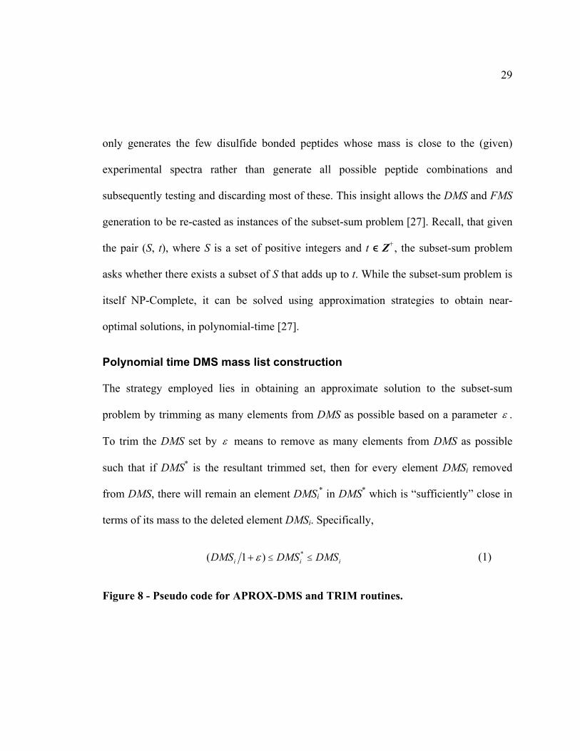
Polynomial time DMS mass list construction

The strategy employed lies in obtaining an approximate solution to the subset-sum

problem by trimming as many elements from DMS as possible based on a parameter .

To trim the DMS set by means to remove as many elements from DMS as possible

such that if DMS* is the resultant trimmed set, then for every element DMSi removed

from DMS, there will remain an element DMSi* in DMS* which is “sufficiently” close in

terms of its mass to the deleted element DMSi. Specifically,

iii DMSDMSDMS *)1( (1)

Figure 8 - Pseudo code for APROX-DMS and TRIM routines.

30

The approximation algorithm for creating the partial DMS is described by the

APPROX-DMS and TRIM routines (Figure 8). APPROX-DMS takes the following

parameters: (1) a sorted list of cysteine-containing peptides mass values (CCP), (2) a

target mass value from the PMS list (PMSval), (3) the trimming parameter , and (4) the

Initial Match threshold (TIM). In lines 2-8 of Figure 8, all the variables and data structures

are initialized. In lines 9-11, the theoretical disulfide-bonded peptide structures are

formed and stored in a temporary set called TempSet. Line 10 excludes values greater

than the PMSval plus a constant corresponding to the Initial Match threshold. The

rationale behind this threshold is explained in the following section. In other words, the

conditional clause in line 10 filters peptide combinations that will not generate any

feasible initial match. Line 12 increments the DMS by invoking the routine MERGE,

31

which returns a sorted set formed by merging the two sorted input sets DMS and

TempSet, with duplicated values removed. In line 13, the TRIM routine is called to

shorten the DMS set. Lines 14-15 examine if the largest mass value in the constructed

DMS set is sufficiently close to the targeted mass PMSval. If so, an Initial Match occurs.

Table 2 presents an example showing the effectiveness of the APROX-DMS. In

this specific case, 37.5% of the entire search space (all feasible combinations of cysteine-

containing peptides) was successfully trimmed, while ensuring that the correct IM was

not missed. Another example illustrating the action of APPROX-DMS on the Beta-LG

protein is available in Appendix A.

Table 2 – Running APROX-DMS on the ST8SiaIV C142-C292 bond. CCP: the mass values of all cysteine-containing peptides. PMSval: a disulfide-bonded precursor ion mass. TrimSet: all the disulfide-bonded structures trimmed from the set of feasible combinations of cysteine-containing peptides. For this example, 37.5% of the structures were trimmed and the correct IM was found.

Property Value

CCP

{716, 728, 749, 863, 864, 891, 976, 1096, 1105, 1161, 1204, 1274, 1359,

1367, 1418, 1480, 1593, 1733, 1754, 1846, 1863, 1864, 1976, 2179, 2292,

2351, 2617, 2737, 2822}

PMSval {2640} (Precursor M+H+ mass and charge state: 2638.121 3)

0.02530

TIM 1.0

TrimSet

{716, 863, 1096, 1443, 1589, 1590, 1611, 1725, 1832, 1838, 1844, 1853,

1866, 1888, 1909, 1958, 1995, 2001, 2022, 2051, 2066, 2070, 2086, 2094,

2107, 2135, 2164, 2178, 2221, 2248, 2249, 2307, 2333, 2363, 2462, 2519}

IM {2640} (KTCAVVGNSGILL – ATRFCDEIHLY) – SS-bond: C142-C292

32

The complexity of both routines MERGE and TRIM is O(|DMS|+|TempSet|) and

O(|DMS|), respectively. Further, for any fixed 0 , our algorithm is a (1+ )-

approximation scheme. That is, for any fixed 0 , the algorithm runs in polynomial

time. The proof of the polynomial time complexity of APPROX-DMS can be obtained by

direct analogy to the proof of the polynomial time complexity of the subset sum

approximation algorithm from [27] and is outlined in Appendix B.

Parameters Estimation

APPROX-DMS depends on two important parameters, namely, the match

threshold TIM and the trimming parameter . The match threshold is responsible for

defining a “matching window”. This is necessary due to practical considerations such as

the sensitivity of the instrument (i.e. 0.01Da, 0.1Da, and 1.0Da) and experimental noise,

due to which an exact match is a rarity. An empirical study was conducted by using

different values of TIM for all the datasets. Based on the results, the TIM value of Da0.1

was found to minimize missing matches as well as the occurrence of false positives.

Considering the smallest precursor ion mass involved, in these studies, the above value of

TIM guaranteed a matching accuracy of 99.86%.

The second parameter is much more important as it is crucial to the running

time of the algorithm and its accuracy as evident from Eq. (1). To determine , we note

33

that it is inversely proportional to the algorithm’s running time. However, a large value of

would cause meaningful fragments to be left out of the DMS. At the same time, a small

value for will lead to few data points being trimmed. Thus “guessing” appropriate

values of can be complicated and suboptimal choices can significantly impact the

quality of the results. This problem of data-driven estimation of is addressed using a

regression framework where is treated as a dependent variable and based on the data, a

functional relationship is obtained between it and the other (independent) variables. This

functional relationship is modeled using the following independent variables: (1) the

cysteine-containing peptides (CCP) mass range defined by CCPmax and CCPmin

corresponding to the peptides with the highest and lowest mass respectively. (2) The

number of cysteine-containing peptides k. A large k implies that the average difference in

the mass of any two peptide fragments is small. Conversely, a small k implies fewer

fragments with putatively larger differences in their masses. (3) The cysteine-containing

peptides average mass value CCPaverage. The relationship between and these other

variables is then obtained using multiple-variable regression. In these studies, the data for

the regression was obtained using bootstrapping where groups of four proteins were

randomly picked from the set of 9 proteins available to us. The functional relationship

defining was obtained to be:

23minmax2 109094.3100824.1103939.1

kCCP

CCPCCP

average

(2)

34

Polynomial time FMS construction

In creating the FMS, a strategy similar to the one used for generating the DMS can

be used. This involves using an approximation algorithm, this time, to generate the

theoretical spectra for all the IMs found during the first-stage matching. Another

trimming parameter is defined to trim the FMS mass list. It can be expected that the

functional form of depends on the fragments mass range, as well as their granularity

(extent to which fragments are broken down into smaller ions). In a manner similar to the

case for estimating ε, a multiple-variable regression was used to obtain the specific

functional form for the dependent variable in terms of the variables AAmax (the largest

amino acid residue mass), AAmin (the smallest amino acid residue mass), AAaverage (the

average amino acid residues mass), and ||p|| (average number of amino acid residues per

fragment). Bootstrapping was once again utilized, resulting in the relationship shown in

Eq. (3).

23minmax3 100731.5100936.3101744.6

pAA

AAAA

average

(3)

Figure 9 - Pseudo code for APROX-FMS routine.

35

The pseudocode of the APPROX-FMS procedure used for generating the FMS is

shown in Figure 9. The function GENFRAGS(.), in line 7, generates multiple fragment

ions (a, b, bo, b*, c, x, y, yo, y*, and z) for peptide sequences in Pepsequences, which contains

the disulfide-bonded peptides involved in the IM being analyzed. Next, for each element

in the FMS and for each fragment in the FragSet (lines 8-11), new disulfide-bonded

peptide fragment structures are formed. Line 10 rejects values greater than the TMSval

(also considering the Validation Match threshold), since they cannot generate any

feasible validation match. In line 12, the current FMS set is combined with the disulfide-

bonded peptide fragments set TempSet using MERGE. In line 13, the FMS is trimmed

using the TRIM routine. Lastly, a Validation Match VM is declared (lines 14-15) when a

36

correspondence is found between the mass of the largest value in FMS and an

experimentally determined mass value TMSval, given a Validation Match threshold.

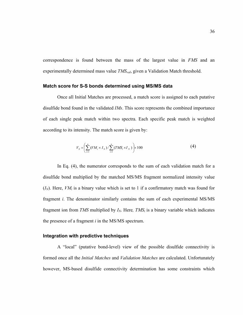
Match score for S-S bonds determined using MS/MS data

Once all Initial Matches are processed, a match score is assigned to each putative

disulfide bond found in the validated IMs. This score represents the combined importance

of each single peak match within two spectra. Each specific peak match is weighted

according to its intensity. The match score is given by:

100)(/)(11

n

iNi

n

iNiS ITMSIVMV (4)

In Eq. (4), the numerator corresponds to the sum of each validation match for a

disulfide bond multiplied by the matched MS/MS fragment normalized intensity value

(IN). Here, VMi is a binary value which is set to 1 if a confirmatory match was found for

fragment i. The denominator similarly contains the sum of each experimental MS/MS

fragment ion from TMS multiplied by IN. Here, TMSi is a binary variable which indicates

the presence of a fragment i in the MS/MS spectrum.

Integration with predictive techniques

A “local” (putative bond-level) view of the possible disulfide connectivity is

formed once all the Initial Matches and Validation Matches are calculated. Unfortunately

however, MS-based disulfide connectivity determination has some constraints which

37

might prevent the method from finding all disulfide bonds in a protein. Among these

limitations, the most impacting one is the presence of blind spots in the MS/MS spectra.

As previously mentioned, blind spots may be caused by intra-chain disulfide bonds,

cross-linked disulfide bonds and circular disulfide bonds. The different types of disulfide

bonds are presented in Figure 10.

Figure 10 – Disulfide bond types. The different S-S bonding types are: (A) inter-chain disulfide bonds, (B) intra-chain S-S bonds, (C) cross-linked disulfide linkages and (D) circular disulfide bonds.

Therefore, a non-MS-based method is necessary to overcome this constraint, since

the presence of blind spots occur due to the strength of disulfide bonds, which prevents

the fragmentation of the protein during mass spectrometry. Amid possible solutions,

predictive techniques were selected to resolve this problem. Motivated by the analysis of

the previous work in this area and by results which demonstrated up to 77% accuracy in

disulfide linkage determination, a support vector machine (SVM) based framework was

implemented.

The framework developed here is based on the work from Chen et al. [19]. In

their studies, a two-level model was used to predict the disulfide connectivity of proteins.

38

Results showed that their SVM-based models outperformed all other predictive

techniques for disulfide connectivity prediction. The main idea underlying their approach

is to combine local and global protein sequence information to train SVM engines, using

the strengths of both. While the local information was encoded by pair-wise methods,

focused on cysteine pairs, global information was encoded by pattern-wise methods,

which took into consideration the different disulfide bonding patterns.

Support Vector Machine (SVM)

Support Vector Machines, or simply SVMs, are a set of supervised learning

methods for the classification of both linear and nonlinear data, based on the analysis of

information and patterns recognition. SVMs are a non-probabilistic binary classifier,

which is a good fit for disulfide bonding determination (since the possible bonding state

can be categorized by just two classes). SVMs use a nonlinear mapping to transform the

original training data into a higher dimension. Within this new dimension, it searches for

the linear optimal separating hyperplane that separates the data into two different classes,

creating a decision boundary. With an appropriate nonlinear mapping to a sufficiently

high dimension, data from two classes can always be separated by a hyperplane. This

hyperplane is found using support vectors and margins [28]. Both entities are represents

in Figure 11.

39

Figure 11 aids in visualization, showing linearly separable 2-D data points, which

are divided by a line into two different classes. If an example addressing 3-D data points

would be used, the data would be divided by a plane. Generalizing to n dimensions, the

data points would be separated by a hyperplane. An SVM approaches this classification

problem by searching the maximum marginal hyperplane. A maximum marginal

hyperplane is defined as the hyperplane with the largest margin. The margin is defined as

the distance (or largest separation) between two classes. The diagonal lines traced in

black in Figure 11 represent the “sides” of the class division and define two supporting

hyperplane. Any data point that falls on these hyperplanes are called support vectors.

That is, any support vector is equally close to the maximum marginal hyperplane (in red).

Figure 11 – SVM: representation of a hyperplane dividing data points with two attributes (2-D). The red line corresponds to the maximum marginal hyperplane. The blue arrow shows the margin, while the support vectors are shown with thicker borders.

40

Although the example above uses 2-D data points to facilitate its understanding,

SVM is capable of handling data with hundreds or even thousands of different

dimensions (attributes). In fact, the SVM trained in this work analyzes data with

hundreds of attributes encoded. The proper and complete training of the SVM used

specifically in the method, together with the different predictive techniques used to

enhance the accuracy of the S-S linkage determination is described next.

SVM-based predictive framework

The fundamental component of properly training a SVM resides in building a

robust, accurate and efficient model, based on the training dataset. The same dataset

extracted from SWISS-PROT database [25] was employed (denoted as SP43) to compare

the framework developed with other approaches [11-12, 18]. A similar filtering

procedure to [7] was applied to ensure only high quality and experimentally verified S-S

41

bond annotations were included. Initially, only the sequences containing information in

the Protein Data Bank (PDB) were included in the filtered dataset. In addition, sequences

with disulfide annotation described as “probable”, “potential” or “by similarity” were

excluded, as well as sequences with more than five disulfide bonds. For cross-validation,

the data was further divided into five subsets. Each subset contained an approximately

equal number of sequences. The entire filtered dataset contains 439 proteins.

The framework developed can be divided in two levels: pair-wise modeling level

and pattern-wise modeling level. Following a similar strategy developed in the MS-based

framework, the second stage aims to validate the results obtained from the first stage. In

the first level, a SVM model infers the disulfide bonding likelihood between any two

cysteines. First, the data were encoded for each possible cysteine pair. For a protein P

with D disulfide bonds, there are D(2D-1) combinations of cysteine pairs (i, j) to be

encoded. The encoded data was generated by two different descriptors: (1) local sequence

profiles around target cysteines and (2) the sequential distance between cysteines

(denoted as DOC).

The sequence profiles were extracted using a window centered at cysteines i and j.

Each residue in the window covering a cysteine was encoded as a vector of 20 elements,

where each element corresponding to an amino acid residue receives a binary value. The

element in the vector associated with the amino acid residue is set to 1, while all the other

42

positions in the vector are set to 0. The window size was set to 13, similarly to the size

used in [19] (which was proved to obtain the best predictive results). Since the sequence

separation between bonded cysteines correlates with specific connectivity patters as

shown in [29], the second descriptor encodes the normalized linear distance between two

cysteines i and j. DOC is defined as , where i and j represent the indices of two

disulfide bonded cysteines. The calculated distance is normalized due to the unitary

characteristic of the encoded sequence profile data vectors. The normalization is obtained

by the equation .

Once the data is fully encoded, each cysteine pair is represented by a vector

containing 521 features (dimensions), combining both sequence profile and DOC

information. Based on all the training vectors, a SVM is trained using LIBSVM [30].

LIBSVM is a library for support vector machines, which allows users to use different

SVM implementations as a tool in their frameworks. In this work, the C-support vector

classification (C-SVC) SVM was used. This formulation was designed for a given set of

training vectors in two different classes [31], which matches the disulfide bond

determination problem. The procedure proposed in [32] was followed to increase the

classification accuracy of the SVM model trained.

43

The scaling of the data was not necessary, since the values of each feature

. Next, all four possible kernel function were tested and, as expected, the radius

based function (RBF) kernel produced the best results. This kernel nonlinearly maps data

into a higher dimensional space being able to handle the case when the relation between

class-labels (true or false disulfide bond) and attributes (vector features) is nonlinear.

RBF required two parameters denoted as C and γ. The parameter C represents the penalty

parameter used by the C-SVC SVM formulation, while the parameter γ is used in the

RBF kernel function. A detailed description of the SVM formulae and other advantages

of the RBF kernel are discussed in [30, 32].

The selection of both parameters C and γ are crucial for the success of the SVM

model classification. Therefore, a grid-search was carried on C and γ using 5-fold cross-

validation to define the best values for each parameter. The values found to optimize the

results of the RBF kernel trained are: and . Lastly, the two

classes studied (whether there exist a disulfide bond or not) are unbalanced as generally

there are much less disulfide bonds formed in a protein than the total number of possible

disulfide bonds. The problem is solved by the addition of a factor (weight) denoted as w

used to increase the penalty parameter C for the pairs classified as non-disulfide bonded.

44

After exhaustively testing different values for w, the best results were found when any

value in the range of was used.

With the SVM formulation selected, the optimal kernel chosen and all the

required parameter defined and calculated, a SVM model was trained based on 439

proteins. This model is then used by the pair-wise modeling stage to calculate the

probability estimate of the occurrence of a S-S bond in every cysteine pair i and j

classified.

In the second (pattern-wise) modeling level, the S-S determination is tackled from

a global perspective. In this scenario, the framework performs two distinct steps: (1)

filters the S-S bonded pairs found in the first stage using the disulfide connectivity

obtained by the MS-based framework (global information). (2) It also uses cysteine

separations profiles [16] (CSPs) to find similar disulfide connectivity patterns between

the different possible bonding arrangements (in analysis) and the training dataset (439

proteins). The filtering step removes all S-S bonded pairs classified in the first stage

which conflict with the disulfide bonds found by the MS-based framework. This filtering

is based on the fact that the predictive techniques are used to fill in the limitations of the

mass spectrometry data. In fact, this filtering procedure reduced considerably the number

of false positives found by the predictive framework.

45

Next, the method calculates the different cysteine separations profiles for the

protein in analysis, considering all possible combinations of bonded pairs resulting from

the filtering in the previous step. Possessing all different CSPs, the framework performs a

CSP search. This search compares the CSPs calculated with the CSPs of all the proteins

in the training dataset and returns the most resembled cysteine separations profile found

for each CSP considered.

Match score for S-S bonds determined using predictive techniques

Each modeling stage aforementioned generates a score for each disulfide bond

predicted. The SVM model used to classify disulfide bonds in the pair-wise stage

calculates a probability indicating the potential of bonding for each disulfide bond

classified. This probability can be further interpreted as how confident the first stage is

toward the prediction. A confidence score is calculated in Eq. 5, where pbond is the

probability estimate for the bonding arrangement and exp(.) is the exponential function.

This function is used to decrease the number of false positives, since it maximizes the

higher pbond values found, due to its exponential growth.

(5)

For the pattern-wise modeling stage, the score is calculated using Eq. 6 from [19],

where D is the divergence between two cysteine separations profiles. The score SCSP is

46

inversely proportional to the divergence D. When a perfect CSP match is found (D = 0),

the score SCSP is maximum (SCSP = 1).

(6)

The overall match score for disulfide bonds determined using the predictive

framework developed is calculated by Eq. 7.

(7)

Determining the globally consistent bond topology

Once all putative S-S bonds are identified using both MS-based method and

predictive techniques, they need to be integrated to obtain a globally consistent view. The

approach to this problem is motivated by Fariselli and Casadio [7]. Specifically, the

location of the putative disulfide bonds is modeled by edges in an undirected graph G (V,

E), where the set of vertices V corresponds to the set of cysteines. To each edge, a match

score (calculated in the previous sections) is assigned. The most probable disulfide

connectivity is found by solving the maximum weight matching problem for the graph G.

A matching M in the graph G is a set of pair-wise non-adjacent edges; that is, two edges

do not share a common vertex. A maximum weight matching is defined as a matching M

that contains the largest possible sum of the weights of each possible edge. For this, the

47

implementation of the Gabow algorithm [33] designed in [34] is used. The final protein’s

disulfide linkage is then converted to a user friendly graphical format in which the entire

protein primary sequence is illustrated and the disulfide bonds are highlighted.

Results

The proposed method was validated utilizing experimental data obtained using a

capillary liquid chromatography system coupled with either a Thermo-Fisher LCQ ion

trap or a LTQ ion trap mass spectrometer LC/ESI-MS/MS system. Details of the

experimental protocols can be found in [35-39]. This work used data from nine

eukaryotic glycosyltransferases. These molecules and their Swiss-Prot ID are: ST8Sia IV

[Q92187], Beta-lactoglobulin [P02754], FucT VII [Q11130], C2GnT-I [Q09324],

Lysozyme [P00698], FT III [P21217], β1-4GalT [P08037], Aldolase [P00883], and Aspa

[Q9R1T5].

Six sets of experiments were conducted to investigate the proposed method and its

efficacy. These experiments included: (1) Analysis of method’s efficiency, showing how

the method successfully reduced the DMS and FMS search spaces. (2) Analysis of the

effect of incorporating multiple ion types, demonstrating the importance of considering

non-b/y ions in the determination of disulfide bonds. (3) Analysis of the effect of

integrating the predictive framework with the MS-based framework, showing that the

48

former contributed positively to the overall method’s accuracy. (4) Comparative analysis

of the proposed method with established predictive techniques. (5) Comparative analysis

of the method with MassMatrix, an established MS-based approach which can be used

for determining S-S bonds. In both experiment 4 and experiment 5, the aforementioned

set of glycosyltransferases and their known S-S bond topology provided the ground truth.

(6) Analysis of the method in terms of established performance measures: Accuracy (Q2),

Sensitivity (Qc), Specificity (Qnc), and Matthew’s correlation coefficient (c).

Analysis of efficiency of the search

One of the most important characteristics of the proposed method is its efficiency

in terms of excluding significant portions of a large and rapidly expanding search space.

In Table 3 the size of the complete DMS (containing all the disulfide-bonded peptide

structures generated for each protein) and the complete FMS (containing all the disulfide-

bonded fragment ions) are compared with the truncated DMS and FMS obtained using the

proposed approach.

Table 3 - DMS and FMS mass space sizes comparison

Protein Disulfide

Bond

Full Search (exponential)

Proposed Search (polynomial) DMS

decrease FMS

decrease DMS size

FMS size

DMS size FMS size

Beta-LG C82C176 2152 2169 1870 78 13.1% 96.4%

ST8Sia IV C142C292 1246 1792 1038 106 16.7% 94.1% C156C356 1246 2640 1038 255 16.7% 90.3%

49

FucT VII C318C321 581 115 528 34 9.1% 70.4% C68C76 879 103 681 41 22.5% 60.2%

C211C214 879 1819 681 107 22.5% 94.1%

B1,4-GalT C134C176 2149 1189 1127 77 47.6% 93.5% C247C266 2149 5480 1127 426 47.6% 92.2% Average DMS and FMS decrease 21.8% 86.4%

It may be noted that across the molecules, on an average, the proposed approach

required examining about 78% of the entire DMS and only about 14% of the entire FMS.

It is crucial to note that this reduction in search was achieved without impacting the

accuracy and having considered all multiple fragment ion types (a, b, bo, b*, c, x, y, yo, y*,

and z). The DMS decrease was less than the FMS decrease because the disulfide-bonded

structures in the DMS were bigger and fewer in number and consequently dispersed

across the spectra mass range. In Figure 12, the actual time taken to obtain a solution by

generating the complete DMS and FMS is analyzed, as well as their truncated

counterparts, for each of the molecules.

Figure 12 – Comparison of the computational time (in seconds) for the exhaustive and partial generation of DMS and FMS of the proteins from Table 3. On average there was a 49.5% decrease in time to compute the DMS and 88.7% decrease in time to compute the FMS. The computations were carried out on an Intel T2390 1.86 GHz single-core processor with 1GB RAM.

50

Effects of incorporating multiple ion types: A case study

In this experiment, the effect of incorporating multiple ion types (a, b, bo, b*, c, x,

y, yo, y*, and z) in determining the S-S bonds as opposed to considering only b/y-ions are

investigated. It was found that multiple instances of combinations between b/y ions and

other ions types occurred by analyzing the confirmatory matches for the different

disulfide bonds. These combinations are available in the Appendix C.

The consideration of multiple ion types also contributed to the method’s accuracy

in terms of determining specific S-S bonds. Disulfide bonds previously missed due to

their low match score could be identified when all ten different ion types were

considered. The tryptic-digested protein FucT VII (which underwent CID) constituted

one such example. In FucT VII the bond C318-C321 was missed when considering only b/y

ions (match score 29, pp=11, pp2 =15). However, as shown in Figure 13, this bond was

51

identified when multiple ions types were included (match score 100, pp=31, pp2=70).

The confidence measures pp and pp2 are described in the Comparative studies with

MassMatrix section.

Figure 13 – Spectra samples from tryptic digested protein FucT VII Spectra (m/z vs. normalized intensity) illustrating the confirmatory matches (whose intensity values were at least 10% of the maximum intensity) found for the disulfide bond between cysteines C318-C321 in protein FucT VII. The spectrum in the left shows the matches found when multiple ions were considered. The spectrum in the right shows the matches when only b/y-ions were considered.

The disulfide bond C318-C321 is used to explain this improvement. This bond is an

intra-bond involving cysteines that are close together. Consequently, CID-based

fragmentation was poor and the consideration of other ion types essentially improved the

signal-to-background contrast. In this particular case, five other ion types - a4, a5, a6, bo

7,

y*7 - were present in the FucT VII MS/MS data besides the b ions represented in the

spectrum on the right in Figure 13. In the following, details of how these ions contribute

to the match score Vs (from Eq. (4)) are reviewed. Two cases are presented: consideration

52

of only b/y-ions (Eq. (8)) and consideration of multiple ion types (Eq. (9)). The

numerator specifies the contribution of each spectrum peak from Figure 13 (the ion

corresponding to each Ni IVM term is showed in brackets).

8.281007321.6

9414.1100

7321.6

][4324.1][1574.0][1732.0][1784.0 7654

bbbb

VS (8)

0.1001002173.67321.6

1007321.6][5797.3][1464.0][1996.0][6787.0

][1863.0][4324.1][1574.0][1732.0][1784.0

7*

765

47654

ybaa

abbbbV

oS (9)

It was also observed that the consideration of multiple ion-types led to significant

increase in the match scores of the true disulfide bonds, whereas only a modest increase

was noticed for false positives. This allowed the increase of the threshold used on the

match score Vs to identify high-quality matches from 30 to 80 (a 166% increase). The

positive effect of this increment on the specificity of the method can be illustrated by

considering the protein Aldolase. In this molecule, consideration of only b/y ions led to a

false positive S-S bond identification between cysteines C135-C202 (Vs=30.8, with

(original) threshold 30). However, when the multiple ions-types were considered with the

(increased) threshold on the match score, no S-S bond was found between C135-C202 (Vs=

53.2, (incremented) threshold 80).

53

Effects of integrating the predictive framework with the MS-based

framework

The integration of the predictive framework to the methodology designed and

implemented allowed the identification of two disulfide bonds that were missed when

only the MS-based framework was used. The combination of both state-of-the-art

techniques (MS-based and predictive) allowed this work to achieve a very high accuracy,

missing just one disulfide bond in 17 true positives for seven different proteins. Its

specificity also became remarkable, since just one true negative S-S bond was missed.

The two newly disulfide bonds predicted were: (1) an intra-bond in the Beta-LG protein

which could not be found due to a blind spot caused by the same intra-bond, making the

protein’s fragmentation difficult. (2) One disulfide bridge in the C2GnT-I protein which

could not be found since the precursor ion cannot be formed by chymotryptic digestion,

which was the digestion carried for C2GnT-I.

Comparative studies with predictive techniques

In this experiment the proposed method was compared with three well known

predictive methods DiANNA [12], DISULFIND [11], and PreCys [18]. The results from

each of the methods are shown in Table 4 along with the with the known disulfide bond

linkages according to the Swiss-Prot knowledgebase. As it can be seen, in terms of

correct identifications (as well as minimizing false positives), the proposed approach

outperformed all the predictive techniques.

54

Table 4 – Comparison with predictive methods

Protein Known Pattern Proposed Algorithm DiANNA 1.1 DISULFIND PreCys

ST8Sia IV C142C292,

C156C356, C142C292, C156C356 C11C156,C142C292,C169C356 None

C142C356,

C156C292

Beta-LG C82C176,

C122C135 C82C176, C122C135 C12C137, C82C176, C126C135 None None

FucT VII

C68C76,

C211C214,

C318C321

C68C76, C211C214,

C318C321 C68C321, C76C211, C214C318 C76C318

C68C76,

C211C214,

C318C321

Β1,4-GalT C134C176,

C247C266 C134C176, C247C266 C23C176, C30C144, C266C341 None

C134C247,

C176C266

C2GnT-I

C59C413,

C100C172,

C151C199,

C372C381

C59C413, C100C172,

C151C199, C372C381

C13C172, C59C217, C151C234,

C199C372, C381C413 Not supported

C59C381,

C100C372,

C151C172,

C199C413

Lysozyme C24C145,

C48C133

C24C145, C48C133,

C24C145, C48C133, C82C98,

C94C112

C24C145, C48C133,

C82C98, C94C112 C82C145

FT III C81C338,

C91C341 C81C338 C16C91, C81C143, C129C338 None C81C91

Aldolase None None C73C339, C135C290, C115C240,

C178C202 None None

Aspa None None C4C275, C60C217, C66C151,

C123C145 None None

Comparative studies with MassMatrix

At the state-of-the-art, MS2Assign [20] and MassMatrix [24] are two MS-based

methods that can be applied to the problem of determining S-S bond connectivity. In the

work of Lee and Singh [3], the MS2DB system developed was found to be comparable to

MS2Assign [20], albeit, in limited testing. Since the proposed method improves upon

MS2DB, only detailed comparative results with MassMatrix [24] is shown in Table 5. As

55

part of this experiment, for each S-S bond, in addition to the empirical match score (Eq.

(4)), a probability based scoring model proposed in [6] was implemented. This model

provided two scores called pp and pp2 scores. The pp score helps to evaluate whether the

number of VMs could be a random. The pp2 score evaluates whether the total abundance

(intensity) of VMs could be a random. A detailed description and formulae of the pp and

pp2 scores is presented in [6]. The reader may note that the proposed method had better

pp and pp2 scores when compared to MassMatrix (higher pp and pp2 scores are better,

indicating smaller p-values). While the match scores (Vs) and (Vp) obtained with the

proposed method were also higher than those obtained with MassMatrix (V*s), no

inferences should be drawn as these scores are calculated differently in each of these

methods. As can be seen from Table 5, every bond correctly determined by MassMatrix

was also found by the method proposed in these studies. However, there were S-S bonds

that were found by the proposed method but not by MassMatrix.

Table 5 - Comparison with MassMatrix. In brackets, (1) the scores (Vs) of each disulfide bond and the confidence scores (pp and pp2 values) for the S-S bonds found by the MS-based framework and (2) the scores (Vp) and their components (SSVM and SCSP) of each disulfide bond found by the predictive framework.

Protein Known Pattern Proposed Method MassMatrix

ST8Sia IV C142C292, C156C356 C142C292 [Vs:131;pp:109;pp2:41],

C156C356 [Vs:100;pp:97;pp2:6]

C142C292 [V*s:54;pp:15;pp2:13],

C156C356 [V*s:77;pp:23;pp2:15]

Beta-LG C82C176, C122C135 C82C176 [Vs:100;pp:49;pp2:16],

C122C135 [Vp:7.09;SSVM:6.37;SCSP:0.72] C82C176 [V*

s:68;pp:14;pp2:14]

FucT VII C68C76, C211C214, C68C76 [Vs:105;pp:41;pp2:98], C68C76 [V*s:12;pp:9;pp2:3],

56

Quantitative assessment and analysis of the method’s performance

If the set of disulfide bonds are denoted by P and the set of cysteines not forming

disulfide bonds by N, then true positive (TP) predictions occur when disulfide bonds that

exist are correctly predicted. False negative (FN) predictions occur when bonds that exist

are not predicted as such. Similarly, a true negative (TN) prediction correctly identifies

cysteine pairs that do not form a bond. Finally, a false positive (FP) prediction,

incorrectly assigns a disulfide link to a pair of cysteines, which are not actually bonded.

Based on these definitions, the following four standard measures were used to analyze the

proposed method.

Sensitivity (Qc) = PTP (10)

C318C321 C211C214 [Vs:100;pp:13;pp2:20],

C318C321 [Vs:100;pp:31;pp2:70]

C211C214 [V*s:78;pp:16;pp2:11],

C318C321 [V*s:46;pp:28;pp2:16]

Β1,4-GalT C134C176, C247C266 C134C176 [Vs:100;pp:61;pp2:29],

C247C266 [Vs:195;pp:88;pp2:177]

C134C176 [V*s:34;pp:9;pp2:7],

C247C266 [V*s:31;pp:7;pp2:7]

C2GnT-I C59C413, C100C172,

C151C199, C372C381

C59C413 [Vs:158;pp:237;pp2:61],

C100C172 [Vp:15.03;SSVM:14.48;SCSP:0.55],

C151C199 [Vs:100;pp:93;pp2:15],

C372C381 [Vs:100; pp:81;pp2:79]

None

Lysozyme C24C145, C48C133

C24C145 [Vs:140;pp:65;pp2:88],

C48C133 [Vs:100;pp:62;pp2:55],

C82C94 [Vp:10.15;SSVM:9.53;SCSP:0.62]

C48C133 [V*s:135;pp:51;pp2:33]

FT III C81C338, C91C341 C81C338 [Vs:100;pp:179;pp2:93] None

Aldolase None None None

Aspa None None None

57

Specificity (Qnc) = NTN (11)

Accuracy (Q2) = NPTNTP (12)

Matthew’s correlation coefficient (c) = ))()()(( FNTNFPTNFPTPFNTP

FNFPTNTP

(13)

Table 6 presents the results obtained for the method developed. With maximum

specificity and high accuracy (99% average), the method correctly reported the

connectivity for most of the proteins. The method only failed to identify one cross-linked

bond in the FT III protein because this particular connectivity configuration creates a

large disulfide-bonded structure, which is poorly fragmented by tandem mass

spectrometry. It was also not identified by the predictive framework. It is important to

note that neither MassMatrix nor MS2Assign were able to this disulfide bridge.

Table 6 - Sensitivity, specificity, accuracy and Mathew’s correlation coefficient results for all nine proteins analyzed.

Protein Qc Qnc Q2 c

ST8Sia IV 1.00 1.00 1.00 1.00

Beta-LG 1.00 1.00 1.00 1.00

FucT VII 1.00 1.00 1.00 1.00

C2GnT-I 1.00 1.00 1.00 1.00

Lysozyme 1.00 0.96 0.96 0.80

Β1,4-GalT 1.00 1.00 1.00 1.00

FT III 0.50 1.00 0.94 0.69

Aldolase X 1.00 1.00 X

Aspa X 1.00 1.00 X

58

Software

The integration of both state-of-the-art MS-based and predictive frameworks was

consolidated in the newly released application MS2DB+. MS2DB+ is a platform-

independent web application that efficiently determines the disulfide linkage in proteins

based on mass spectrometry data and machine learning techniques. The software can

account for multiple ions (a, b, bo, b*, c, x, y, yo, y*, and z) in determining the disulfide

bonds. It also uses a SVM-based model and cysteine separations profiles to increase the

disulfide connectivity prediction accuracy. MS2DB+ is publicly available at:

http://tintin.sfsu.edu/~whemurad/disulfidebond/. Its source code is accessible at

http://code.google.com/p/disulfidebond/ under the Apache License 2.0.

Implementation

MS2DB+ was coded in PHP and currently runs on an Apache web server. PHP is

a widely-used general-purpose scripting language that is especially suited for web

development. Apache is the most popular HTTP server available, becoming the first web

server software to surpass the 100 million web site milestone, according to a web server

survey conducted by Netcraft in 2009. In MS2DB+, the disulfide bond determination can

be done in two modes: standard analysis (completely automatic) and advanced analysis

(user may customize thresholds and parameters).

59

Both of these modes require three inputs: (a) a ZIP file containing any of the

standard file formats used to store mass spectrometry data (i.e. mzXML, mzML, mzData

or Sequest DTA files), (b) the protein sequence in FASTA format and (c) the protease

used to digest the protein sample. Other non-standard file formats generated by different

tandem MS/MS methods can be converted to one of the acceptable file formats using the

open-source framework ProteomeCommons.org IO, created by Jayson Falkner and freely

available at (www.proteomecommons.org/current/531/).

XML-based file formats became the standard open-source data formats for

storage and exchange of mass spectrometry data. The Extensible Markup Language

(XML) aids to the simplicity, generality and usability of the data. It allows research

groups from all over the world to use the same set of rules for encoding MS information,

opening the possibility of a common file format for MS data exchange worldwide.

Initially developed by the SPC/Institute for Systems Biology, mzXML is one of

the most common formats of mass spectrometry data exchange. It provides a container

for MS and MS/MS proteomics data. Another significant advantage is the fact that most

of the raw, proprietary file formats from most mass spectrometer vendors can be

converted to the open mzXML format. mzData was developed by the Human Proteome

Organization (HUPO) and offers similar functionalities to mzXML. mzML is the mass

spectrometry data format developed by the Mass Spectrometry Standards Working Group

60

of the HUPO Proteomic Standards Initiative (HUPO-PSI). mzML is the combined effort

of research centers and instrument vendors worldwide to replace the currently most used

mzXML and mzData formats by a single XML-based format.

The utilization of the predictive framework in the determination of disulfide

connectivity can be easily triggered in both modes. This novel and powerful integration is

activated by a single user click. Users can choose whether or not to include predictive

techniques in the analysis of S-S linkage. If both frameworks are turned on, the

application distinguishes the disulfide bonds found by showing the different match scores

Vs and Vp for each bond, as well as a note depicting the S-S bridges found by the SVM-

based predictive framework.

The key parameters users can customize include: initial and confirmatory

matching thresholds, MS/MS intensity/abundance threshold which contributes to

suppressing MS-data noise, and the trimming parameters ε and δ, which are used to trim

the theoretical spectra during the Initial and Confirmatory Matching stages respectively.

Optionally, in both interfaces, the user may also (a) choose different combinations of

multiple ion types to be considered during the spectral matching (based on knowledge of

the dissociation method); (b) select the number of missing cleavage sites during protein’s

digestion; and (c) specify the protein region where a disulfide bond is not expected to

occur.

61

Usage Example

Here, a walkthrough demonstrating the use of MS2DB+ using the protein

Syalyltransferase ST8Sia IV (UniProt ID Q92187) is described. This example is one of

nine Glycosyltransferases with varying S-S bonding topologies, the MS/MS data for

which have been made available in the Datasets page of the MS2DB+ site.

As a first step, in the standard analysis page (Fig.14.A), the user needs to upload a

ZIP file containing the corresponding set of data file(s), enter the protein’s FASTA

sequence and select the protease used during digestion. Next, MS2DB+ analyzes the data

and lists the disulfide bonds found with either (1) their empirical and statistical scores

calculated for S-S bonds found by the MS-based framework or (2) their empirical scores

SSVM and SCSP combined for the disulfide bridges found by the SVM-based framework.

Each bond is shown graphically, as in Fig.14.B where two bonds (C142-C292 and C156-

C356) are shown. MS2DB+ also provides other relevant information for each disulfide

bond found by the MS-based framework, including (1) the disulfide-bonded peptide

structure and the data file involved in the initial match, (2) a graph containing the most

abundant spectral matches (Fig.14.D), (3) the list of confirmatory matches along with the

fragment ions matched (theoretical and experimental), (4) their respective mass values

and mass difference (both measured in Daltons), and (5) the fragments charge state (z)

and the peaks normalized intensity (abundance) (Fig.14.C). Each confirmatory match

62

whose normalized intensity (abundance) is found to be equal or greater than 50% is

highlighted in green to facilitate rapid identification.

Figure 14 - (A) The standard analysis interface of MS2DB+ showing the key inputs for the molecule ST8SiaIV. (B) Disulfide bonds (in yellow) found for ST8SiaIV. (C) Some of the confirmatory matches found for the S-S bond between cysteines C142-C292. Matches whose MS/MS fragment’s normalized intensity equal or exceed 50% are marked in green). (D) The confirmatory spectrum for an initial match (in red) containing the most abundant confirmatory peaks found while determining the S-S bond between cysteines C142-C292.

Conclusions

An algorithmic methodology combining a MS-based framework and a predictive

SVM-based framework was presented for determining S-S bond topologies of molecules.

The method uses MS/MS data and machine learning techniques based on pair-wise and

pattern-wise disulfide linkage information. The proposed approach is computationally

63

efficient, data driven, and has high accuracy, sensitivity, and specificity. It is not limited

either by the connectivity pattern or by the variability of product ion types generated

during the fragmentation of precursor ions. Furthermore, the approach does not require

user intervention and can form the basis for high-throughput S-S bond determination. The

complete method developed here was fully implemented and is publicly available at

http://tintin.sfsu.edu/~whemurad/disulfidebond. The web application created is called

MS2DB+.

References

1. Singh R: A review of algorithmic techniques for disulfide-bond

determination. Briefings in Functional Genomics and Proteomics, 2008, 7(2),

pp. 157-172.

2. Nesvizhskii AI, Vitek O, Aebersold R: Analysis and validation of proteomic

data generated by tandem mass spectrometry. Nature Methods, 2007, 4(10),

pp. 787-797.

3. Lee T, Singh R: Comparative Analysis of Disulfide Bond Determination Using

Computational-Predictive Methods and Mass Spectrometry-Based

Algorithmic Approach. BIRD, CCIS 13, 2008, pp. 140-153.

4. Johnson RS, Martin SA, Biemann K, Stults JT, Watson JT: Novel fragmentation

process of peptides by collision-induced decomposition in a tandem mass

64

spectrometer: differentiation of leucine and isoleucine. Anal Chem, 1987,

59:2621

5. Steen H, Mann M: The abc’s (and xyz’s) of peptide sequencing. Nature

Reviews, Molecular Cell Biology, 5, 2004, pp.699-711

6. Xu H, Freitas MA: A mass accuracy sensitive probability based scoring

algorithm for database searching of tandem mass spectrometry data. BMC

Bionformatics 2007, 8:133-142

7. Fariselli P, Casadio R: Prediction of disulfide connectivity in proteins.

Bioinformatics 2001, 17, 957-64.

8. Fariselli P, Riccobelli P, Casadio R, Role of evolutionary information in

predicting the disulfide-bonding state of cysteines in proteins, Proteins, 36,

1999, 340-346

9. Fariselli P, Martelli PL, Casadio R, A neural network base method for

predicting the disulfide connectivity in proteins, Knowledge based Intelligent

Information Engineering Systems and Allied Technologies KES, 2002, Vol. 1,

IOS Press, p 464-468

10. Vullo A, Frasconi P, Disulfide connectivity prediction using recursive neural

networks and evolutionary information, BIOINFORMATICS, Vol. 20 no. 5

2004, pages 653–659 DOI: 10.1093/bioinformatics/btg463

65

11. Ceroni A et al: DISULFIND: A Disulfide Bonding State and Cysteine

Connectivity Prediction Server. Nucleic Acids Research 2006; 34:177-181.

12. Ferre F, Clote P: DiANNA: A Web Server for Disulfide Connectivity

Prediction. Nucleic Acids Research 2005; 33:230-232.

13. Ferre F, Clote P, Disulfide Connectivity prediction using secondary structure

information and diresidue frequencies, Bioinformatics, Vol. 21, No. 10, 2005,

2336-2346, doi:10.1093/bioinformatics/bti328

14. Altschul SF, et al, Gapped BLAST and PSI-BLAST: a new generation of

protein database search programs, Nucleic Acid Research, 1997, Vol. 25, No.

17, 3389-3402

15. Jones DT, Protein secondary structure prediction based on position-specific

scoring matrices, J. Mol Biol. 292195-202, 1999

16. Zhao E, et al, Cysteine separations profiles on protein sequences infer

disulfide connectivity, BIOINFORMATICS, Vol. 21 no. 8 2005, pages 1415–

1420 doi:10.1093/bioinformatics/bti179

17. Chen YC, Hwang JK, Prediction of Disulfide Connectivity from Protein

Sequences, PROTEINS: Structure, Function, and Bioinformatics 61, 2005, 507-

512

18. Tsai CH et al: Improving disulfide connectivity prediction with sequential

distance between oxidized cysteines. Bioinformatics 2005, 21:4416-4419

66

19. Chen BJ, Tsai CH, Chan CH, Kao CY, Disulfide Connectivity Prediction with

70% Accuracy Using Two-Level Models, PROTEINS: Structure, Function, and

Bioinformatics 64:246–252, 2006

20. Schilling B et al: MS2Assign, automated assignment and nomenclature of

tandem mass spectra of chemically crosslinked peptides. J Am Soc Mass

Spectrom., 14(8):834-50, 2003

21. Yu ET, et al.: The Collaboratory for MS3D: A New Cyberinfrastructure for

the Structural Elucidation of Biological Macromolecules and Their

Assemblies Using Mass Spectrometry-Based Approaches. J Proteome Res.

(2008). ASAP article, 10.1021/pr800443f

22. Lee T, Singh R, Yen TY, Macher B: An Algorithmic approach to Automated

High-Throughput Identification of Disulfide Connectivity in Proteins Using

Tandem Mass Spectrometry. Proc. Computational Systems Bioinformatics,

CSB, 2007, pp. 41-51

23. Lee T, Singh R, Yen R, Macher B: A mass-based hashing algorithm for the

identification of disulfide linkage patterns in protein utilizing mass

spectrometry data. Proc. IEEE International Symposium on Computer-Based

Medical Systems, CBMS, 2007, pp. 397-402

24. Xu H, Zhang L, Freitas MA: Identification and Characterization of Disulfide

Bonds in Proteins and Peptides from Tandem MS Data by Use of the

67

MassMatrix MS/MS Search Engine. Journal of Proteome Research, 7, 13-144,

2008.

25. Bairoch A, Apweiler R, The SWISS-PROT protein sequence database and its

supplement TrEMBL in 2000, Nucleid Acid Research, 2000, Vol. 28, No. 1, 45-

48

26. American Society for Mass Spectrometry [http://www.asms.org]

27. Cormen TH, Leiserson CE, Rivest RL, Stein C: Introduction to Algorithms, 2nd

edition, MIT Press, Cambridge, MA, U.S.A, 2001

28. Han J, Kamber M: Data Mining – Concepts and Techniques, 2nd edition, Morgan

Kaufmann Publishers, San Francisco, CA, U.S.A, 2006

29. Harrison PM, Sternberg MJE, Analysis and classification of disulphide

connectivity in proteins, J Mol Biol, 39: 4207-4216, 1994

30. Chang CC, Lin CJ, LIBSVM: a library for support vector machines, 2001

31. Vapnik V, The nature of statistical learning theory, New York, Springer, 1995

32. Hsu CW, Chang CC, Lin CJ, A Practical Guide to Support Vector Machine,

2003

33. Gabow HN: An efficient implementation of Edmonds’ Algorithm for

Maximum Matching on Graphs. Journal of the ACM, 23, 2006, 221-234

34. Rothberg E, MATHPROG: Solver for the maximum weight matching

problem [http://elib.zib.de/pub/Packages/mathprog/matching/weighted/]

68

35. Thomas S, Yen TY, Macher BA: Eukaryotic glycosyltransferases: cysteines

and disulfides. Glycobiology, 12, 2002, pp. 4G-7G

36. Yen TY, Macher BA: Determination of glycosylation sites and disulfide bond

structures using LC/ESI-MS/MS analysis. Methods in enzymology 2006;

415:103-113

37. Angata K, Yen TY, El-Battari A, Macher B, Fukuda M, Unique Disulfide Bond

Structures Found in ST8Sia IV Polysialyltransferase Are Required for Its

Activity, The Journal of Biological Chemistry, VOL. 276, No. 18, May 4, 2001,

pp. 15369-15377

38. Yen TY, Macher BA, Bryson S. et al, Highly Conserved Cysteines of Mouse

Core 2 β1,6-N-Acetylglucosaminyltransferase I Form a Network of Disulfide

Bonds and Include a Thiol That Affects Enzyme Activity, J Biology

Chemistry, Vol. 278, No. 46, Issue 14, 45864-45881, 2003

39. Thomas S, Yen TY, Macher BA, Eukaryotic glycosyltransferases: cysteines

and disulfides, Glyco-Forum Section, 2001

40. Murad W, Singh R, Yen TY, An efficient algorithmic approach for mass

spectrometry-based disulfide connectivity determination using multi-ion

analysis, BMC Bioinformatics, 2010

69

41. Murad W, Singh R, Yen TY: Polynomial-Time Disulfide Bond Determination

Using Mass Spectrometry Data. Proc. IEEE Computational Structural

Bioinformatics Workshop, CSBW, 2009, 79-86

42. Chen T, Jaffe JD, Church GM: Algorithms for Identifying Protein Cross-links

via Tandem Mass Spectrometry. Proc. RECOMB, 2001, pp. 95-102

43. Frank A, Tanner S, Pevzner P: Peptide Sequence Tags for Fast Database

Search in Mass-Spectrometry. Proc. RECOMB 2005, LNBI 3500, pp. 326-341,

2005

44. Keller A, Nesvizhskii AI, Kolker E, Aebersold R: Empirical statistical model to

estimate the accuracy of peptide identification made by MS/MS database

search. Analytical Chemistry, 74(20), 2002

45. Mackenzie HA, Ralston GB, Shaw DC, Location of sulfhydryl and disulfide

groups in bovine beta-lactoglobulins and effects of urea, Biochemistry VOL.

11, November, 1972, pp. 4539-4547

46. de Vries T, et al, Neighboring cysteine residues in human fucosyltransferase

VII are engaged in disulfide bridges, forming small loop structures,

Glycobiology, VOL. 11, No. 5, December 12, 2000, pp. 423-432

47. Baldi P, Cheng J, Vullo A, Large-scale prediction of disulphide bond

connectivity, Advances in Neural Information Processing Systems 17.

Cambridge, MA: MIT Press, 2005, p 97-104

70

48. Platt J, Probabilistic outputs for support vector machines and comparison to

regularized likelihood methods, Advances in Large Margin Classifiers,

Cambridge, MA: MIT Press, 2000

49. Chen YC, Lin YS, Lin CJ, Hwang JK, Prediction of the bonding states of

cysteines using the support vector machines based on multiple feature

vectors and cysteine state sequences, Proteins, 55, 2004, 1036-1042

50. Fiser A, Simon I, Predicting the oxidation state of cysteines by multiple

sequence alignment, Bioninformatics, 16, 2000, 251-256

51. Martelli PL, Fariselli P, Malaguti L, Casadio R, Prediction of the disulfide-

bonding state of cysteines in proteins at 88% accuracy, Protein Sci., 11, 2002,

2735-2739

52. Lu CH, Chen YC, Yu CS, Hwang JK, Predicting Disulfide Connectivity

Patterns, PROTEINS: Structure, Function, and Bioinformatics, 67, 2007, 262-

270

53. Ward JJ, McGuffin LJ, Buxton BF, Jones DT, Secondary structure prediction

with support vector machines, Bioinformatics, 19, 2003, 1650-1655

54. Abkevich VI, Shakhnovich EI, What can disulfide bonds tell us about protein

energetics, function and folding?: simulations and bioinformatics analysis, J

Mol Biol, 300, 2000, 975-985

71

55. Wedemeyer WJ, Welker E, Narayan M, Scheraga HA,Disulfide bonds and

protein folding, Biochemistry, 39, 2000, 4207-4216

56. Chuang CC, et al, Relationship between protein structures and disulfide-

bonding patterns, Proteins, 53, 2003, 1-5

57. Frasconi P, Passerini A, Vullo P, A Two-Stage SVM Architecture for

Predicting the Disulfide Bonding State of Cysteines, Proc. of the IEEE

Workshop in Neural Networks for Signal Processing, 2002, 25-34

58. Cheng J, Saigo H, Baldi P, Large-scale prediction of disulphide bridges using

kernel methods, two-dimensional recursive neural networks, and weighted

graph matching, Proteins, 62, 2006, 617-629

59. Lenffer J, Lai P, Mejaber WE, et al, CysView: Protein Classification Based on

Cysteine Pairing Patterns, Nucleic Acid Research, 32, 2004, 350-354

60. Hogg PJ, Disulfide bonds as switches for protein function, Trends Biochem

Sci, 28, 2003, 210-214

61. Matsumura M, Signor G, Matthews BW, Substantial increase in proteins

stability by multiple disulfide bonds, Nature, 342, 1989, 291-293

62. Craig R, Krokhin O, Wilkins J, et al, Implementation of an algorithm for

modeling disulfide bond patterns using mass spectrometry, J Proteome Res, 2,

2003, 657-661

72

63. Bafna V, Reinert K, Mass spectrometry and computational proteomics,

Encyclopedia of Genetics, Genomics, Proteomics, and Bioinformatics. John

Wiley & Sons, 2005

64. Gorman JJ, Wallis T, Pitt JJ, Protein disulfide bond determination by mass

spectrometry, Mass Spectrom Rev, 21, 2002, 183-216

65. Morris HR, Pucci P, A new method for rapid assignment of S-S bridges in

proteins, Biochem Biophys Res Commun, 126, 1985, 1122-1128

66. Fenyo D, A software tool for the analysis of mass spectrometric disulfide

mapping experiments, Bioinformatics, 13, 1997, 17-18

67. Fenyo D, Beavis RC, A Method for Assessing the Statistical Significance of

Mass Spectrometry-Based protein Identifications Using General Scoring

Schemes, Anal Chem, 75, 2003, 768-774

68. McAfee KJ, Duncan DT, Assink M, Link AJ, Analyzing Proteomes and Protein

Function Using Graphical Comparative Analysis of Tandem Mass

Spectrometry Results, Molecular & Celular Proteomics, 2006, 1497-1513

69. Wu Z, Lajoie G, Ma B, MSDASH: Mass Spectrometry Database and Search,

CSB, 2008, 63-71

70. Meija J, Mathematical tool in analytical mass spectrometry, Anal Bioanal

Chem, 385, 2006, 486-499

73

71. Mormann M, Eble J, et al, Fragmentation of intra-peptide and inter-peptide

disulfide bonds of proteolytic peptides by nanoESI collision-induced

dissociation, Anal Bioanal Chem, 392, 2008, 831-838

72. Choi S, Jeong J, Na S, Lee HS, et al, New Algorithm for the Identification of

Intact Disulfide Linkages Based on Fragmentation Characteristics in

Tandem Mass Spectra, Journal of Proteome Research, 9, 2010, 626-635

Appendix A

Action of APPROX-DMS on the protein Beta-LG

An example illustrating the action of APPROX-DMS on the Beta-LG protein is

shown below. Table 7 presents snapshots of the DMS, TrimSet, and IM sets for each

CCPi (cysteine-containing peptide) mass value, during each iteration of the trimming

process.

Table 7 - DMS, TrimSet and IM mass sets for each CCPi mass value generated from the tryptic digestion of the protein Beta-lactoglobulin (Beta-LG). The values presented here are retrieved at the end of each loop cycle (lines 5-13) in Figure 4.

i CCPi DMS TrimSet IM

0 1064 {0,1064} {} {}

1 1192 {0,1064, 1192, 2254} {} {}

2 1658 {0, 1064, 1192, 1658, 2254, 2720, 2849} {} {}

3 1746 {0, 1064, 1192, 1658, 1746, 2254, 2720, 2849, 2937} {2809} {}

4 2275 {0, 1064, 1192, 1658, 1746, 2275, 2720, 2849, 2937} {2254, 2809} {}

5 2477 {0, 1064, 1192, 1658, 1746, 2275, 2477, 2720, 2849, {2254, 2809} {}

74

2937}

6 2535 {0, 1064, 1192, 1658, 1746, 2275, 2535, 2720, 2849,

2937} {2254, 2477, 2809} {}

7 2648 {0, 1064, 1192, 1658, 1746, 2275, 2535, 2648, 2720,

2849, 2937} {2254, 2477, 2809} {}

8 2776 {0, 1064, 1192, 1658, 1746, 2275, 2535, 2648, 2776,

2849, 2937} {2254, 2477, 2720, 2809} {}

9 2790 {0, 1064, 1192, 1658, 1746, 2275, 2535, 2648, 2776,

2849, 2937}

{2254, 2477, 2720, 2790,

2809} {}

10 2930 {0, 1064, 1192, 1658, 1746, 2275, 2535, 2648, 2776,

2849, 2937}

{2254, 2477, 2720, 2790,

2809, 2930} {}

11 3189 {0, 1064, 1192, 1658, 1746, 2275, 2535, 2648, 2776,

2849, 2937, 3189}

{2254, 2477, 2720, 2790,

2809, 2930} {3189}

Appendix B

Etudes of the proof of polynomial complexity

The proof that the proposed method is a fully polynomial approximation scheme

consists of two parts. First, we need to show that each value returned by the APPROX-

DMS function is within 1 from the optimal solution. Second, we need to show that

the running time of the method is fully polynomial. We refer the reader to [27] for the

proof of the first part and focus in the following on analyzing the complexity of the

method. To show that the method is a fully polynomial-time approximation scheme, we

derive a bound on the length of a DMS set. After trimming, successive elements

iDMS and 'iDMS of DMS must have a relationship 1'

ii DMSDMS . Therefore, each

75

possible DMS set contains up to valPML1log values. Since xxxx 1ln1 and

10 , it can be shown that:

valvalvalval

PMSPMSPMSPML

ln2ln1

1ln

lnlog1

(11)

As can be seen from Eq. (11), this bound is (explicitly) polynomial in the size of

the input valPMS . It is also (implicitly) polynomial in the size of the set DMS since is

directly proportional to the number of cysteine-containing peptides k (per Eq. (2)) and

these peptides are in turn combined to form each element of the DMS . A similar

argument can be made for the APPROX-FMS routine, completing thereby the proof that

the proposed method is a fully polynomial-time approximation scheme.

Appendix C

Combination between b/y ions and other ions types on MS/MS data

In the following, we show that combinations between ion types other than just b

and/or y ions do occur, even for proteins that underwent CID. Most importantly, many of

these combinations were present with high abundance across the proteins we analyzed.

Table 8 - Different combinations of multiple ion types present in some of the proteins we used to validate the method proposed. For each protein, we present all combinations involving ion types other than just b and/or y ions, whose normalized

76

intensity (or abundance) was found to be at least 50% of the highest intensity value measured.

Protein Disulfide

Bonds

Confirmatory matches

(each match is presented as a [ion types; abundance measured] pair)

ST8Sia IV C142C292 [b*

3bo

5; 56%], [b*3a7; 100%], [c4b

o5; 80%], [b5y

o12; 62%]

C156C356 [z7b*

5; 66%], [a8b*4; 75%], [a8a4; 69%], [y4a10; 63%]

Beta-LG C82C176 [a10; 68%], [c11; 51%], [x5y*6; 58%], [x5y14; 100%], [b6c13; 68%], [c8y

*14; 66%]

FucT VII

C68C76 [y*7; 57%], [a5a15; 100%], [b*

7b*14; 57%]

C211C214 [bo9; 75%]

C318C321 [z7; 100%], [y*7; 95%]

Β1,4-GalT C134C176 [a18; 63%], [b*

7a18; 76%]

C247C266 [c5c24; 100%]

C2GnT-I

C59C413 [b*

14; 100%], [x7y*7; 84%], [z3y

o11; 56%], [z3y

*11; 79%], [a16; 77%], [z6c16;

77%], [y9c18; 93%], [x16y13; 79%]

C372C381 [c6x8; 100%], [x23; 52%], [c9a20; 100%], [c6bo22; 98%], [c6b

*22; 50%]

C151C199 [a9; 100%], [a3c9; 51%], [b*

7bo10; 72%], [b*

7y9; 100%], [a3b*14; 65%], [b*

4a14;

78%]

Lysozyme C24C145 [x3a6; 100%]

C48C133 [x2yo

4; 100%], [a11; 50%]