Distributed Solar Adoption in Orlando:A household-level model for distribution resource planning

Sam Koebrich, Ben Sigrin, Robert Spencer, Paul Schwabe, Scott Haase – NRELSam Choi, Justin Kramer – Orlando Utilities CommissionJanuary 2021 | NREL PR-6A20-77308

NREL | 2

Disclaimer

This work was authored in part by the National Renewable Energy Laboratory, operated by Alliance for Sustainable Energy, LLC,for the U.S. Department of Energy (DOE) under Contract No. DE-AC36-08GO28308. Funding provided by Orlando Utilities Commission under Agreement TSA-18-01146. The views expressed herein do not necessarily represent the views of the DOE, the U.S. Government, or the Orlando Utilities Commission.

This analysis presents projections of distributed solar adoption completed jointly with NREL and the Orlando Utility Commission (OUC) for the OUC service territory. The results were developed using the NREL dGen model, which simulates the technical, economic, and behavioral factors affecting consumers’ adoption decisions. See https://www.nrel.gov/analysis/dgen/and https://github.com/nrel/dgen for more detail.

NREL | 3

Overview

• Technical potential for rooftop solar in Florida is massive, offsetting 47% of retail sales (3rd overall nationally)1, yet adoption lags (12th

nationally) 2. A 2018 Florida Public Service Commission ruling3

authorizing solar third-party ownership (leasing) has increased attention on distributed solar.

• Orlando (pop. 292k) has committed to a 100% clean-energy target by 2050. Deployment of solar and storage are expected to contribute significantly to reaching the goal.

• Deployment of customer-adopted solar, unlike utility-procured solar, is uncertain, but known to be spatially correlated with demographic factors and existing adoption.

• Bottoms-up solar adoption forecasting methods at the household-level are integral to long-term resource planning by anticipating system needs as customers increasingly adopt distributed solar, storage, electric vehicles, and other distributed energy resources.

Projected distributed solar adoption at the building-level for the OUC service territory, facilitating long-term integrated resource (IRP) and distribution resource planning (DRP)

1 Gagnon et al 2016; 2 – WoodMac 2020; 3 – Florida PSC 2018

NREL | 4

Key Findings

• Using LiDAR rooftop scans we estimate 2.9 GWDC of rooftop solar technical potential in OUC. By 2050, and based on current retail tariffs, the median performing owner-occupied single-family household could economically offset 47% of their annual electricity consumption (41.5% on the peak load day).

• Under the Baseline scenario, 370 MW is projected by 2050, primarily in the residential sector (343 MW) rather than C&I (24 MW). Across scenarios, much of the growth occurs by 2035. Adoption is sensitive to both rate reform (-72%) and lower PV costs (+62%). The Net Billing (-74%) component drives most of the reduction in adoption in the rate reform scenario.

• A substantial fraction of OUC’s solar technical (26%) and economic potential is on residential multi-family or renter-occupied buildings, which have historically adopted at lower rates than other segments.

• This study developed a new method to i) represent building-level agents in adoption forecasts and ii) train a predictive model to estimate probabilities in the dGen model1 considering locational peer-effects. Using an agent-based modeling approach, adoption predictions are aggregated by OUC distribution feeder, finding substantial differences. For instance, 25% of all projected adoption through 2050 would be concentrated on just 5% of feeders and 88% of projected adoption on 50% of feeders. This study did not examine if any distribution system upgrades would be needed or introduce any hosting capacity limits considering this adoption potential. 1 Sigrin et al. 2016

NREL | 5

Substantial Differences in Adoption Levels by Distribution Feeder

Adoption by Top 20 Feeders (MW)

Feeder ID1 2020 2030 2040 2050

A 1.7 16.5 21.4 23.2B 1.2 15.7 20.6 22.3C 0.9 11.7 15.6 17.1D 0.4 6.2 10.1 16.5E 0.9 9.4 13.7 15.5F 0.6 8.7 13 15.3G 1.4 9.4 12.8 14.5H 0.8 8 12 12.6I 0.8 7.7 10.5 12J 0.7 6.3 8.7 10.8K 0.6 5.9 8.1 9L 0.5 5.9 8.2 8.8M 0.9 5.7 8 8.8N 0.4 6.4 8.1 8.6O 0.7 5.6 8.1 8.6P 0.5 5.9 8 8.3Q 0.4 5.8 7.6 7.9R 0.2 4.5 6.6 7.9S 0.2 4.4 6.5 7.8T 0.4 4.8 6.8 7.7Figure: Projected rooftop solar adoption (MW) by distribution feeder

in Baseline scenario in 2050 1 – Actual IDs were redacted

NREL | 6NREL | 6

Outline 1. Methodology and Data2. Results

• Technical potential• Economic potential • Projection of adoption by feeder, sector, scenario,

and year

3. Conclusions 4. Appendix A: Methods for Rooftop

Assessment

Methodology and Data

NREL | 8NREL | 8

Takeaway This analysis uses LiDAR roof scans, customer level electricity consumption, property assessment, and other data to provide a solar adoption forecast at the household level.

We use the dGen tool, an agent-based model that assesses each agent’s technical, economic, and adoption potential in order to create an adoption projection.

NREL | 9

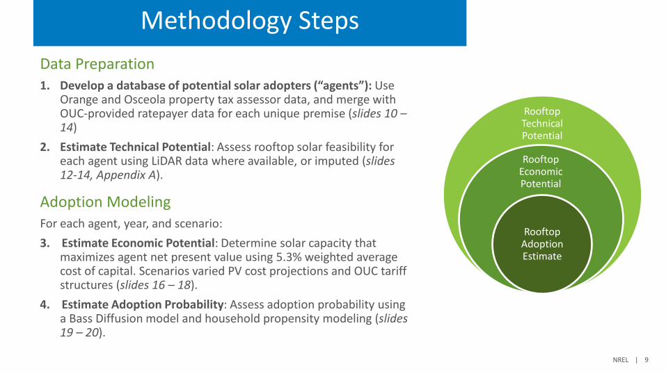
Data Preparation1. Develop a database of potential solar adopters (“agents”): Use

Orange and Osceola property tax assessor data, and merge with OUC-provided ratepayer data for each unique premise (slides 10 –14)

2. Estimate Technical Potential: Assess rooftop solar feasibility for each agent using LiDAR data where available, or imputed (slides 12-14, Appendix A).

Adoption ModelingFor each agent, year, and scenario:3. Estimate Economic Potential: Determine solar capacity that

maximizes agent net present value using 5.3% weighted average cost of capital. Scenarios varied PV cost projections and OUC tariff structures (slides 16 – 18).

4. Estimate Adoption Probability: Assess adoption probability using a Bass Diffusion model and household propensity modeling (slides 19 – 20).

Rooftop Technical Potential

Rooftop Economic Potential

Rooftop Adoption Estimate

Methodology Steps

NREL | 10

This study was novel for using the dGen model with an “agent” database resolved at the premise-level. To do this, we increased the specificity of rooftop area suitable for solar, the correlation between a building’s electrical consumption profile and its roof suitability, socio-demographic attributes of the building occupants, and peer effects from existing solar adoption in OUC. These model developments improve the spatial precision of adoption forecast.

Previous dGen Studies

vs.

This Study

Representation of OUC consumers as statistically-representative agents sampled

from probability distributions

Representation of OUC consumers as individuals with their unique,

actual attributes

Update to Methodology

Methods:

Data Preparation

NREL | 12

Data Coverage

OUC Customers

LiDAR Coverage~ 43.27%

Parcels Coverage99.96%

Three datasets are used to compile the agent database:

1) Complete file of OUC customers; 2) Orange and Osceola county tax

assessor parcels (99.9% coverage)3) LiDAR partial scan (2016) of the OUC

territory to infer rooftop suitability at the building level (43.3% coverage).

NREL | 13

LiDAR Methodology

LiDAR data is used to detect attributes of each roof plane based on developable area, tilt angle, and azimuth. These are passed to the NREL PVWATTS model to simulate annual and hourly generation for each roof plane.

LiDAR measurements are present for 43% of buildings in OUC territory. Thus, a model was trained to predict suitable roof area for remaining buildings (56.7%), primarily on building coverage, or the ratio of developable area to building footprint. The model is validated by demonstrating that probability density function of the inferred roofs’ area, tilt, and azimuth match that of the measured data. See slide 22-26 for results and Appendix A for methods.

NREL | 14

Associating Agents with Distribution Feeders

The OUC provided feeder-level geographic data as underground and overhead lines, which are then converted to polygons and mapped to agents based on their locations.

Methods:

Adoption Modeling

NREL | 16

Spatial extent: OUC service territory, for each premise

Retail rate growth: Based on historic trends (2.75% escalation per year)Load growth: Based on 2020 Integrated Resource Plan (1.4% escalation per year). This study does not explicitly consider new building construction nor changes in patterns of electricity consumption.

Sectors: • Residential single family owner-occupied (n = 59,355)• Non-residential owner-occupied (n = 6,834)

• Residential multi-family (n = 9,157)• Residential single-family rental (n = 31,486) • Commercial rental (n = 4,928)

Study Parameters

Assessed for technical, economic, and adoption potential, but not included in final projection

NREL | 17

Scenarios

Scenario Name Costs Retail Rates

Current Tariff Mid-Cost

Mid PV costs(NREL ATB 2018)

Current OUC tariffs, escalating at 2.75%/yearNet metering1 extended through 2050

Current Tariff Low-Cost

Low PV costs(NREL ATB 2018)

Current OUC tariffs, escalating at 2.75%/yearNet metering1 extended through 2050

Reformed Tariff Mid-Cost

Mid Costs Residential: Transition to TOU tariffs: On-peak: $0.191/kWh (2 – 8pm)Off-peak: $0.055/kWh (all other hours)

Non-Residential: No tariff change

Net billing: hourly excess solar generation compensated at avoided cost ($30/MWh in 2020, escalating to $45/MWh by 2050)

Reformed Tariff Low-Cost

Low Costs

Net Billing Mid-Cost Mid Costs Current OUC tariffs, escalating at 2.75%/year.Net billing: hourly excess solar generation compensated at a flat avoided cost ($30/MWh in 2020, escalating to $45/MWh by 2050)

Net Billing Low-Cost Low Costs

Baseline

Identifies impact of cost reduction

Identifies impact of Net Billing alone

Identifies impact of Net Billing and Time of Use

1 Net Metering involves ‘crediting’ exported generation at the retail rate, utilizing credits to offset future generation. dGen does not ‘oversize’ systems to produce generation in excess of annual consumption.

NREL | 18

Financial ModelingEach agent completes a discounted cash flow analysis in each model year. The cash flows include capital and O&M costs, revenue from bill savings and the ITC, and tax considerations (i.e. MACRS). Electricity bill savings is based on hourly solar generation and electricity consumption profiles. Adoption is based on a customer owned system, rather than third party operators.

Costs (NREL Annual Tech Baseline 2018):2018

– Residential $2,640/kW– C&I : $1,810/kW

2050 – Mid-Cost Residential $1,140/kW– Mid-Cost C&I : $963/kW– Low-Cost Residential $560/kW– Low-Cost C&I : $522/kW

Economic ParametersRetail rates (based on current tariffs)Residential agents evaluate the Residential Electric Service tariff and Commercial agents the General Electric Service or GES Secondary tariffs depending on max demand. Rates escalate at 2.75% (nominal) per year.

Financing ParametersAgents use a 5.3% WACC, with a 20% down payment for purchase, which is used to calculate NPV. Financing assumptions are based on the NREL 2018 Annual Technology Baseline, which is benchmarked to industry trends. Agents have equal financing attributes to simplify comparison, though in practice households have different access and cost of financing.

NREL | 19

Using consumer surveys, we relate the system payback to the fraction of consumers that would adopt solar.1,2 Agents use a 5.3% WACC as the economic criteria in evaluating the optimal system size. Non-residential agents behave more conservatively and require lower payback periods to adopt.

Maximum market share is paired with a Bass Diffusion model to simulate aggregate adoption over time. The aggregate adoption is then disaggregated to individual agents based on their predicted probability (see next slide)

These values used to estimate market adoption (deployment) from economic potential

How Much Solar is Adopted?

1 Dong & Sigrin 2019; 2 Paidipati et al. 2008

NREL | 20

Agent Propensity ModelingAgent-level probability of adoptionEquation 1 is used to calculate agent-level probability of adoption (π). It is a reformulation of the Bass diffusion model for discrete agents. Probability is influenced by technology innovators (p), imitators (q), and the level of territory-wide saturation (a) relative to the estimated maximum market penetration (m) by sector.

• π is the probability that agent will adopt in each time increment (bi-annual). π is bounded by 0 when a > m

• p and q are the OUC-wide coefficients of innovation and imitation by sector. Estimated with regression on historic adoption.

• m is the sum of each agent’s calculated maximum market share (slide 19), by sector• a is the cumulative count of adopters to date, by sector and year.• π is bounded by 0 when a > m, or the observed adoption exceeds the maximum market

Update probabilities with zip code-level peer effects

Next, probability of adoption is updated to reflect zip code-level peer effects. Given an array of agent probabilities (π) for a given year, we apply a weight based on the number of adopters in the last year within their zip-code. At each time step, and for each sector, we calculate a histogram of zip-codes by the adoption within the zip-code as a percent of all adoption. We then standardize these percentage bins to have a mean of 1, and multiply these weights based on the zip-code and sector of each agent’s probability.

Results

Figure shows downtown Orlando with LiDAR-inferred roof suitability

NREL | 22NREL | 22

Takeaway 2.9 GWDC of solar PV are technically viable within the OUC service territory. Of which, 648 MW is economically developable by 2030 under the Current Tariff Mid-Cost scenario. From this, about 248 MW could be adopted by 2030, increasing to 370 MW by 2050.

Moving from a net-metering to net-billing tariff significantly reduced the projected adoption from 248 to 46 MW by 2030.

NREL | 23

Technical potential is the amount of capacity that could be installed across all developable roofs. This number increases over time as the efficiency of PV modules improves and as more buildings are built.

LiDAR data was used to assess developable area net of shading, tilt, and orientation exclusions, assuming a 160 W/m2 efficiency. Panel efficiency is modeled to linearly increase to 300 W/m2 in 2050

See Appendix A for more detail

Rooftop Solar Technical Potential

Sector Developable Customers (n) Developable Roof Area (million-ft2) Technical Potential (MW)

C&I – Rental 4,928 37.1 551

C&I – Owner Occupied (Homestead) 6,864 40.7 606

Res – Single Family Owner Occupied 59,355 66.6 991

Res – Multi-Family 9,157 20.6 306

Res - Single Family Renter Occupied 31,486 29.5 439

Total (Owner-Occupied Buildings Only) 66,219 107.4 1,596

Total (All Buildings) 111,790 194.5 2,891

NREL | 24

Generation Potential and ConsumptionThe choice of system size by an agent tends to fall into three categories:

• Agents who do not find it economic to adopt solar

• Agents who can adopt a system that offsets some of their consumption.

• Agents who can adopt solar that offsets 100% of their annual consumption (dGen does not oversize systems).

For most (57%) eligible agents in 2020, it is either not technically feasible or economic to adopt solar PV. For 19% of agents it is economic to adopt a system that offsets some percent of annual electricity consumption. Finally 24% of agents have a large enough roof and would find it economic to size of PV system that offsets their entire consumption on an annual basis, though not for each individual hour (top right).

Next we show the percentage of annual electricity consumption that can be offset by the technical potential, by the amount of economic solar potential, and of the amount of adoption (right). Potential should be interpreted as instantaneous and not cumulative (e.g. 20% of system load could be economically offset in 2030). Intuitively, the amount of offset that is economic is less than the technical fraction, but is higher than the offset by projected adoption.

Technical potential decays as system load growth outpaces improvements in solar PV cell efficiency. Economic potential is highly sensitive to changes in the federal Investment Tax Credit (ITC) and gradual declines in solar costs. Adoption potential follows an ‘S-Curve’ of adoption, diffusing into the maximum market potential.

NREL | 25

Generation Potential on Peak Day

We estimate the potential for DPV to offset hourly consumption during OUC’s peak load day (August 15th) using weather data from a typical meteorological year. In the Baseline scenario in 2050 adopted DPV generation might offset 7.5% of annual system electricity consumption (2.16 GWh / 28.8 GWh). Amongst adopters, the median residential adopter might offset 42% of their consumption and commercial adopters 89%. Note that this only considers offsets during the peak load day, not peak hour, and does not consider changes in the shape or timing of load.

Results:

Economic Potential

NREL | 27

Economic potential is the instantaneous amount of PV capacity (MW) that exceeds the agent’s required rate of return (5.3%). Economic potential declines after the ITC expiration and increases long-term as PV costs decline.

In 2030 we model 648 MW of economic potential for owner-occupied buildings (647 MW residential, 1.2 MW C&I). By 2050, economic potential increases to 1,111 MW.

Model results also indicate substantial potential for renter-occupied and multi-family buildings, and that solar is uneconomic for most C&I customers in the near term. This suggests commercial adoption to date could be fueled by non-economic reasons, (e.g. green branding). Non-residential OUC customers tend to offer higher payback periods due to lower costs of electricity than the residential sector.

Economic Potential Results

NREL | 28

Payback Period is the number of years for system revenue to exceed the system costs. This metric is used to convert economic potential into estimated market shares based on customer survey results.

Payback periods (top left) are impacted by the expiration of the ITC, however they stabilize by 2030 due to assumed declines in technology cost. Paybacks differ by agent (bottom left) due to differences in agents’ roof orientations, rate structures, and electricity consumption.

Payback Period Results

Solar-Developable Load (GWh)

Weighted-Average Payback Period (years)

NREL | 29

This heat map shows one pixel per agent modeled in 2030, with color corresponding to system capacity.

Economic potential in this slide includes all sectors.

Pockets of economic potential––particularly for larger systems–– exist near Holden Heights, Lee Vista Blvd, and scattered throughout downtown.

Where is distributed solar economical in OUC?

Results:

Solar Adoption

NREL | 31

Under the Current Tariff Mid-Cost scenario, 370 MW is projected by 2050, primarily in the residential sector (343 MW) rather than C&I (24 MW)1. Much of the growth, across scenarios, occurs by 2035.

Adoption in 2050 is sensitive to both rate reform (-72%) and lower PV costs (+62%). The Net Billing (-74%) component drives the majority of reduction in adoption in the Reform Tariff scenario.

Non-traditional sectors i.e., residential single family rental (162 MW), multi-family (34 MW) and leased commercial (19 MW) could increase deployment by 54%.

Residential adoption is larger than C&I because of differences in value of generation (C&I use a demand charge, v. the residential TOU) and differences in required rates of return by sector (see slide 19)

See slide 38 for full data

Projected Adoption

1 All totals include 3.2 MW of historic adoption from non owner-occupied sectors2 We use FL homestead exemptions to identify whether a single family home is owner-occupied or not.

2

NREL | 32

These figures show a supply curve of the projected solar adoption ranked by the modeled system payback period in 2030 and 2050. A large fraction of the adoption occurs in the residential sector and there is relatively little variance in the threshold payback period.

Relatively little adoption is projected in the C&I sectors because they have i) higher payback periods than residential customers on average; and ii) a higher willingness to adopt threshold. However, prices decline enough to spur C&I adoption by 2050 in the Current Tariff Mid-Cost scenario.

Historic uneconomic adoption

Adoption by Payback Period

NREL | 33

This heat map shows one dot per agent modeled in 2030 and 2050, with color corresponding to the adopted system size. The 2030 and 2050 projections can be compared to identify areas of near-term and long-term growth.

Adoption Heatmap2030 2050

System size (kW)

System size (kW)

NREL | 34

Adoption by Distribution Feeder

Cumulative DPV Adopted (MW) Annual Consumption Offset (%) Peak Day Consumption Offset (%)Feeder ID1 2020 2030 2040 2050 2020 2030 2040 2050 2020 2030 2040 2050

A 1.65 16.5 21.4 23.18 7% 82% 92% 87% 2% 21% 28% 30%B 1.17 15.73 20.65 22.54 7% 84% 95% 91% 2% 23% 31% 34%C 0.92 11.73 15.6 17.07 6% 74% 85% 81% 2% 21% 28% 30%D 0.34 6.23 10.1 16.47 1% 23% 33% 47% 0% 9% 14% 23%E 0.9 9.41 13.65 15.45 7% 64% 80% 79% 2% 18% 26% 30%F 0.6 8.67 13.01 15.34 5% 61% 79% 81% 1% 16% 24% 28%G 0.23 11.18 14.24 14.7 1% 36% 40% 36% 0% 9% 12% 12%H 1.35 9.44 12.77 14.49 7% 64% 76% 75% 2% 20% 28% 31%I 0.75 8 12 12.63 5% 51% 66% 61% 1% 14% 21% 22%J 0.82 7.65 10.49 11.98 5% 59% 71% 71% 1% 18% 25% 29%K 0.67 6.29 8.68 10.87 4% 36% 43% 47% 1% 12% 16% 20%L 0.64 5.93 8.11 8.96 7% 68% 80% 77% 2% 22% 30% 33%M 0.5 5.95 8.2 8.79 5% 52% 61% 58% 1% 13% 18% 19%N 0.86 5.65 7.93 8.72 3% 32% 39% 38% 1% 12% 17% 19%O 0.36 6.39 8.13 8.58 4% 55% 61% 56% 1% 13% 16% 17%P 0.63 5.55 8.09 8.55 4% 36% 45% 41% 1% 13% 19% 21%Q 0.52 5.92 7.99 8.34 5% 51% 59% 54% 1% 14% 19% 19%R 0.38 5.83 7.6 7.94 4% 50% 56% 51% 1% 12% 15% 16%S 0.24 4.51 6.63 7.87 3% 54% 68% 70% 1% 14% 21% 25%T 0.22 4.37 6.52 7.79 2% 33% 43% 44% 0% 9% 13% 16%

Under the Baseline scenario, 7 feeders in 2050 had projected annual DPV generation greater 75% of annual consumption, however no feeder exceeded 35% generation offset on the peak day. Adoption was concentrated, where 25% of all projected adoption through 2050 occurs on 5% of feeders and 88% of projected adoption on 50% of feeders. The study does not consider hosting capacity limits on distribution networks.

1 – Actual IDs were redacted for security reasons

Conclusions

NREL | 36

In the Current Tariff Mid-Cost scenario, 248 MW of rooftop solar PV adoption is projected by 2030, rising to 370 MW by 2050. Most of this adoption is concentrated in the single-family owner-occupied residential sector. This analysis does not include distributed storage or electric vehicle adoption, which could be predicted using a similar approach.

Two modeling sensitivities were evaluated: the cost of solar, and the tariff structure. While a lower cost of PV significantly increased the amount of adoption by 2030 and 2050, tariff reform that replaces net metering with net billing and introduces residential time of use rates reduced adoption by a similar degree.

The detailed spatial resolution of the modeling approach can assist energy planners conducting load forecasting, distribution system planning, or integrated resource planning to anticipate future DER growth.

Conclusions

NREL | 37

Adoption by Scenario and Sector

Adoption in res – renter, res - multifamily, and C&I - leased is simulated using similar logic as the owner-occupied sector but not included in final projection due to landlord-tenant barriers in energy technology adoption

NREL | 38

Adoption by Scenario and SectorScenario Sector 2014 2016 2018 2020 2022 2024 2026 2028 2030 2032 2034 2036 2038 2040 2042 2044 2046 2048 2050

Current Tariff Low-Cost C&I - leased 1.2 1.2 1.5 3.2 4.7 7.0 8.4 12.0 18.9 25.2 32.7 40.4 45.9 50.2 52.2 52.9 53.9 55.7 61.5Current Tariff Low-Cost C&I - owned 1.1 1.1 1.3 2.0 3.6 6.5 10.6 17.9 23.5 27.5 32.7 40.0 44.0 49.1 54.6 55.5 56.5 58.0 59.2Current Tariff Low-Cost res - homestead 1.0 2.6 8.8 30.0 58.6 118.3 208.0 315.5 421.4 489.5 520.5 533.5 537.0 538.0 538.3 538.3 538.4 538.4 538.4Current Tariff Low-Cost res - multifamily 0.3 0.5 0.5 0.9 1.3 2.5 5.1 9.9 18.0 26.5 33.2 35.9 36.8 37.3 37.4 37.5 37.5 37.5 37.5Current Tariff Low-Cost res - rental 0.1 0.3 1.1 5.2 11.5 27.8 58.1 106.3 169.2 216.7 240.1 249.2 251.9 252.7 252.8 252.8 252.8 252.8 252.8Current Tariff Mid-Cost C&I - leased 1.2 1.2 1.5 1.7 1.7 1.7 1.8 1.8 1.8 1.8 1.8 1.8 1.8 2.0 3.2 4.9 8.2 13.3 19.0Current Tariff Mid-Cost C&I - owned 1.1 1.1 1.3 1.6 1.6 1.6 1.6 1.7 1.7 1.7 1.7 1.8 1.8 1.8 2.6 6.5 11.5 18.9 23.6Current Tariff Mid-Cost res - homestead 1.0 2.6 8.8 26.6 35.4 50.5 103.6 176.1 242.6 282.0 300.9 307.3 310.9 314.5 317.8 322.6 328.5 335.0 343.3Current Tariff Mid-Cost res - multifamily 0.3 0.5 0.5 1.4 1.5 1.9 2.7 5.4 8.7 15.2 21.5 26.6 29.4 31.6 32.5 33.3 33.7 34.0 34.3Current Tariff Mid-Cost res - rental 0.1 0.3 1.1 4.5 5.9 9.4 24.4 53.5 96.5 131.4 146.1 150.4 152.2 153.4 154.6 155.6 157.6 159.4 161.9

Net Billing Low-Cost C&I - leased 1.2 1.2 1.5 3.2 4.2 4.5 5.5 6.7 9.4 10.7 13.1 15.7 20.9 26.3 36.6 41.0 47.2 51.2 56.7Net Billing Low-Cost C&I - owned 1.1 1.1 1.3 2.0 2.9 3.5 4.4 5.9 10.8 12.9 16.4 19.1 23.8 28.4 36.5 41.2 47.6 53.3 58.2Net Billing Low-Cost res - homestead 1.0 2.6 8.8 30.0 31.1 33.0 38.9 56.6 100.0 137.2 163.4 185.1 209.3 242.5 270.4 297.3 321.4 340.3 353.8Net Billing Low-Cost res - multifamily 0.3 0.5 0.5 0.9 1.0 1.1 1.3 1.9 3.2 4.9 7.7 10.5 14.8 20.8 24.1 26.7 28.9 30.9 33.6Net Billing Low-Cost res - rental 0.1 0.3 1.1 5.2 5.4 5.7 6.9 11.4 26.6 48.3 72.3 93.9 112.8 129.5 142.8 154.3 165.2 173.5 179.8Net Billing Mid-Cost C&I - leased 1.2 1.2 1.5 1.7 1.7 1.7 1.7 1.7 1.8 1.8 1.8 1.8 1.8 1.9 2.8 3.4 5.1 7.4 10.3Net Billing Mid-Cost C&I - owned 1.1 1.1 1.3 1.6 1.6 1.6 1.6 1.6 1.6 1.7 1.7 1.7 1.7 1.8 2.0 2.3 6.0 8.9 11.5Net Billing Mid-Cost res - homestead 1.0 2.6 8.8 26.6 26.7 26.7 27.3 30.2 41.3 59.6 75.5 79.1 79.4 79.4 79.5 79.6 79.7 79.8 79.8Net Billing Mid-Cost res - multifamily 0.3 0.5 0.5 1.4 1.4 1.4 1.4 1.5 1.7 3.2 4.5 6.1 9.3 10.4 11.1 11.2 11.3 11.4 11.4Net Billing Mid-Cost res - rental 0.1 0.3 1.1 4.5 4.5 4.5 4.7 5.5 9.0 16.4 27.7 34.9 35.9 36.0 36.1 36.2 36.3 36.3 36.3

Reformed Tariff Low-Cost C&I - leased 1.2 1.2 1.5 3.2 4.2 4.5 5.5 6.7 9.4 10.7 13.1 15.7 20.9 26.3 36.6 41.0 47.2 51.2 56.7Reformed Tariff Low-Cost C&I - owned 1.1 1.1 1.3 2.0 2.9 3.5 4.4 5.9 10.8 12.9 16.4 19.1 23.8 28.4 36.5 41.2 47.6 53.3 58.2Reformed Tariff Low-Cost res - homestead 1.0 2.6 8.8 30.0 30.1 30.6 34.0 50.0 95.8 147.1 191.4 223.1 256.9 291.2 316.4 340.0 361.9 378.4 390.7Reformed Tariff Low-Cost res - multifamily 0.3 0.5 0.5 0.9 1.0 1.0 1.3 2.0 3.5 5.3 8.2 11.3 15.7 22.1 25.2 27.2 29.3 31.2 32.5Reformed Tariff Low-Cost res - rental 0.1 0.3 1.1 5.2 5.3 5.4 6.4 10.6 24.8 45.6 70.9 96.0 118.7 138.4 150.7 161.6 171.5 178.0 182.7Reformed Tariff Mid-Cost C&I - leased 1.2 1.2 1.5 1.7 1.7 1.7 1.7 1.7 1.7 1.7 1.7 1.7 1.7 1.8 2.0 2.5 3.7 4.8 7.1Reformed Tariff Mid-Cost C&I - owned 1.1 1.1 1.3 1.6 1.6 1.6 1.6 1.6 1.6 1.6 1.7 1.7 1.7 1.8 2.2 3.0 3.8 5.1 6.6Reformed Tariff Mid-Cost res - homestead 1.0 2.6 8.8 26.6 26.6 26.6 26.6 27.4 31.5 38.3 49.6 62.1 71.0 78.2 81.7 85.0 87.4 90.1 92.9Reformed Tariff Mid-Cost res - multifamily 0.3 0.5 0.5 1.4 1.4 1.4 1.4 1.4 1.6 2.0 2.5 3.0 4.0 5.2 6.4 7.5 8.4 9.5 11.5Reformed Tariff Mid-Cost res - rental 0.1 0.3 1.1 4.5 4.5 4.5 4.5 4.7 5.8 8.0 12.5 19.2 27.1 33.2 36.7 39.5 41.2 42.9 44.6

--- Historic Non Owner-Occupied 1.2 1.2 1.5 3.2 3.2 3.2 3.2 3.2 3.2 3.2 3.2 3.2 3.2 3.2 3.2 3.2 3.2 3.2 3.2

* Sectoral totals may differ from previous cumulative totals due to rounding

NREL | 39

Study LimitationsThis study developed projections of distributed solar adoption in OUC and is subject to limitations in the modeling methodology.These include:

• Principally, modeling results should be understood as projections and not forecasts. That is, the analysis is intended to be comparative across the scenarios and not interpreted as a literal forecast. This includes but is not limited to unforeseen events including economic recessions and changes in policy applicable to distributed solar.

• This study does not consider adoption of other technologies, e.g. electric vehicles or battery storage or their influence on solar adoption

• This study does not consider evolution in patterns of energy consumption, for instance, impacts of electrification. It also doesnot consider future new building construction which could differ from existing buildings in their level of electricity consumption and propensity to include solar during construction

• This study uses credible but uncertain projections of various techno-economic variables as documented in the text, i.e. solar technology cost. Future solar adoption could deviate from these projections depending on the future techno-economic variable values.

• LiDAR data was used to estimate rooftop technical potential, spanning 43% of buildings in OUC service territory. A predictivemodel was used to infer technical potential for the remaining 57% of buildings, including the developable area, tilt, azimuth, and unshaded area. Appendix A documents this process including the goodness-of-fit. The study does not examine sensitivity of model results to the uncertainty in the inferred technical potential.

• Survey results used to associate payback periods with willingness to adopt fractions were taken from previous studies and not reconducted for OUC.

Finally, this study was limited in the number of scenarios considered, and these should not be considered exhaustive of the factors significant to influencing solar adoption.

Appendix A:

Methods for Rooftop Assessment

NREL | 41

Data Coverage

OUC Customers

LiDAR Coverage~ 43.27%

Parcels Coverage99.96%

Three datasets are used to compile the agent database: i) A file of locations of all OUC customers and other details relating to tariff subscription and consumption; ii) Tax assessor appraisals of parcels in Orange and Osceola county (99.9% coverage); iii) A LiDAR partial scan (2016) of the OUC territory, which is to infer rooftop suitability at the building level (43.3% coverage).

OUC Customers

Developable Planes

Building Footprints

Parcel Footprints

From the different data sources we develop a unified agent database. Centroids of the OUC customers do not span the LiDAR assessment. Thus, a GIS spatial intersection is used to merge parcels with the LiDAR measurements.

Mapping Customer “Agents” to Buildings (with Parcels)Raw data Parcels joined with LiDAR

NREL | 43

Data Imputation

LiDAR Footprint Area Distribution (Standardized) Inferred Footprint Area Distribution (Standardized)

LiDAR data is used to assess developable area, tilt and azimuth. However this data only covers roughly 43% of OUC customers. Therefore the developable area is imputed by training a predictive model on the observed data, primarily using building footprint area as an independent variable.

NREL | 44

Data Imputation: Methodology

A. Infer Optimal Developable Coverage (%)Random sampling from “Developable Coverage” distribution stratified by building area percentiles

B. Infer Optimal Developable Area (m2)Developable Coverage * Footprint Area

C. Infer Tilt Angle (degrees)Reverse random sampling from “Developable Coverage” distribution stratified by tilt anglesDistributions provide a probability-weighted choice for the Tilt based on a given percent coverage

D. Infer Azimuth Angle (degrees)Reverse random sampling from “Developable Coverage” distribution stratified by azimuth anglesDistributions provide a probability-weighted choice for the Azimuth based on a given percent coverage

E. Calculate Generation (Capacity Factor 8760 profile)Pre-calculated generation data based on location, tilt, and azimuth.

F. Generation and Developable Area by AgentLookup the capacity factor profile by parcel IDLookup the developable area by parcel ID and divide by number of customers within parcel (typically only 1)

NREL | 45

Data Imputation

LiDAR Developable Coverage

Inferred Developable Coverage

0 – 0.1

0.1 – 0.95

0.95 – 0.99

0.99 – 1

Building Area Percentile

These figures compare the empirical LiDAR data to those inferred by the predictive model. Models are first compared against the building “coverage”, or the ratio of developable area to building footprint. That is, the median building in OUC developable area is approximately 50% of it’s footprint.

The top figures show the probability density function of the empirical data (left, mean = 0.49, std = 0.21) and inferred (right, mean = 0.53, std = 0.21).

The bottom figure shows the PDE for different percentiles of the building area, which visualizes the goodness-of-fit.

LiDAR Tilt Angle Inferred Tilt Angle

Tilt

Angl

e (d

egre

es)

Tilt

Angl

e (d

egre

es)

Data Imputation

0

15

25

35

Tilt Angle (degrees)

45

These figures compare the empirical LiDAR data to those inferred by the predictive model. Models are next compared against the tilt of the primary developable roof plane and the roof coverage, i.e. ratio of developable area to building footprint.

The top figures shows a scatterplot of empirical data (left) and inferred (right). A negative correlation is found between empirical coverage and tilt (ρ = -0.43). Correlation in the inferred data was similar (ρ= -0.45)

The bottom figure shows the PDE for different percentiles of the building area, which visualizes the goodness-of-fit.

LiDAR Azimuth Angle Inferred Azimuth Angle

South (180)

Southwest (225)

Southeast (135)

East (90)

Azimuth Angle

West (270)

Data ImputationThese figures compare the empirical LiDAR data to those inferred by the predictive model. Models are next compared against the azimuth (orientation) of the primary developable roof plane and the roof coverage, i.e. ratio of developable area to building footprint.

The top figures shows a scatterplot of empirical data (left) and inferred (right). A negative correlation is found between empirical coverage and azimuth (ρ = -0.15). Correlation in the inferred data was similar (ρ = -0.14)

The bottom figure shows the PDE for different percentiles of the building area, which visualizes the goodness-of-fit.

NREL | 48NREL | 48

ReferencesDobos, Aron P. 2015. PVWatts Version 5 Manual. Golden, CO: National Renewable Energy Laboratory. NREL/TP-6A20-62641. http://www.nrel.gov/docs/fy14osti/62641.pdf

Dong, C., & Sigrin, B. 2019) Using willingness to pay to forecast the adoption of solar photovoltaics: A “parameterization+ calibration” approach. Energy Policy, 129, 100-110. https://www.sciencedirect.com/science/article/pii/S0301421519301004

Florida Public Service Commission. 2018. Docket No. 0170273-EQ. http://www.psc.state.fl.us/library/filings/2018/03712-2018/03712-2018.pdf

Gagnon, Pieter, Robert Margolis, Jennifer Melius, Caleb Phillips, and Ryan Elmore. 2016. Rooftop Solar Photovoltaic Technical Potential in the United States: A Detailed Assessment. NREL/TP-6A20-65298. https://www.nrel.gov/docs/fy16osti/65298.pdf

NREL (National Renewable Energy Laboratory). 2018. 2018 Annual Technology Baseline. Golden, CO: National Renewable Energy Laboratory. https://atb.nrel.gov/.

Paidipati, J., Frantzis, L., Sawyer, H., Kurrasch, A. 2008. Rooftop Photovoltaics Market Penetration Scenarios. Burlington, MA: Navigant Consulting. NREL/SR-581- 42306. http://www.nrel.gov/docs/fy08osti/42306.pdf.

Sigrin, B., Gleason, M., Preus, R., Baring-Gould, I., & Margolis, R. 2016. Distributed generation market demand model (dGen): Documentation. NREL/TP-6A20-65231. National Renewable Energy Lab.(NREL), Golden, CO (United States). https://www.nrel.gov/docs/fy16osti/65231.pdf

WoodMackenzie. 2020. Q2 2020. U.S. Solar Market Insight. https://www.seia.org/us-solar-market-insight