Distributed localization in wireless sensor networks: a ...koen/papers/compnw.pdf · Distributed localization in wireless sensor networks: a quantitative comparison Koen Langendoen

Computer Networks 43 (2003) 499–518

www.elsevier.com/locate/comnet

Distributed localization in wireless sensor networks:a quantitative comparison

Koen Langendoen *, Niels Reijers

Faculty of Information Technology and Systems, Delft University of Technology, 2828 CD Delft, Netherlands

Abstract

This paper studies the problem of determining the node locations in ad-hoc sensor networks. We compare three

distributed localization algorithms (Ad-hoc positioning, Robust positioning, and N -hop multilateration) on a single

simulation platform. The algorithms share a common, three-phase structure: (1) determine node–anchor distances, (2)

compute node positions, and (3) optionally refine the positions through an iterative procedure. We present a detailed

analysis comparing the various alternatives for each phase, as well as a head-to-head comparison of the complete al-

gorithms. The main conclusion is that no single algorithm performs best; which algorithm is to be preferred depends on

the conditions (range errors, connectivity, anchor fraction, etc.). In each case, however, there is significant room for

improving accuracy and/or increasing coverage.

� 2003 Elsevier B.V. All rights reserved.

Keywords: Ad-hoc networks; Distributed algorithms; Positioning

1. Introduction

Wireless sensor networks hold the promise of

many new applications in the area of monitoring

and control. Examples include target tracking,

intrusion detection, wildlife habitat monitoring,

climate control, and disaster management. The

underlying technology that drives the emergenceof sensor applications is the rapid development in

the integration of digital circuitry, which will bring

us small, cheap, autonomous sensor nodes in the

near future.

* Corresponding author.

E-mail address: [email protected] (K. Langen-

doen).

1389-1286/$ - see front matter � 2003 Elsevier B.V. All rights reserv

doi:10.1016/S1389-1286(03)00356-6

New technology offers new opportunities, but it

also introduces new problems. This is particularly

true for sensor networks where the capabilities of

individual nodes are very limited. Hence, collab-

oration between nodes is required, but energy

conservation is a major concern, which implies

that communication should be minimized. These

conflicting objectives require unorthodox solutionsfor many situations.

A recent survey by Akyildiz et al. discusses a

long list of open research issues that must be ad-

dressed before sensor networks can become widely

deployed [1]. The problems range from the physi-

cal layer (low-power sensing, processing, and

communication hardware) all the way up to the

application layer (query and data disseminationprotocols). In this paper we address the issue of

localization in ad-hoc sensor networks. That is, we

ed.

mail to: [email protected]

500 K. Langendoen, N. Reijers / Computer Networks 43 (2003) 499–518

want to determine the location of individual sensor

nodes without relying on external infrastructure

(base stations, satellites, etc.).

The localization problem has received consid-

erable attention in the past, as many applications

need to know where objects or persons are, andhence various location services have been created.

Undoubtedly, the Global Positioning System

(GPS) is the most well-known location service in

use today. The approach taken by GPS, however,

is unsuitable for low-cost, ad-hoc sensor networks

since GPS is based on extensive infrastructure (i.e.,

satellites). Likewise solutions developed in the

area of robotic [2–4] and ubiquitous computing [5]are generally not applicable for sensor networks

as they require too much processing power and

energy.

Recently a number of localization systems have

been proposed specifically for sensor networks [6–

12]. We are interested in truly distributed algo-

rithms that can be employed on large-scale ad-hoc

sensor networks (100+ nodes). Such algorithmsshould be:

• self-organizing (i.e., do not depend on global in-

frastructure),

• robust (i.e., be tolerant to node failures and

range errors), and

• energy efficient (i.e., require little computation

and, especially, communication).

These requirements immediately rule out some of

the proposed localization algorithms for sensor

networks. We carried out a thorough sensitivity

analysis on three algorithms that do meet the

above requirements to determine how well they

perform under various conditions. In particular,

we studied the impact of the following parameters:range errors, connectivity (density), and anchor

fraction. These algorithms differ in their position

accuracy, network coverage, induced network

traffic, and processor load. Given the (slightly)

different design objectives for the three algorithms,

it is no surprise that each algorithm outperforms

the others under a specific set of conditions. Under

each condition, however, even the best algorithmleaves much room for improving accuracy and/or

increasing coverage.

The main contributions of our work described

in this paper are:

• we identify a common, three-phase, structure in

the distributed localization algorithms.

• we identify a generic optimization applicable toall algorithms.

• we provide a detailed comparison on a single

(simulation) platform.

• we show that there is no algorithm that per-

forms best, and that there exists room for im-

provement in most cases.

Section 2 discusses the selection, generic structure,and operation of three distributed localization al-

gorithms for large-scale ad-hoc sensor networks.

These algorithms are compared on a simulation

platform, which is described in Section 3. Section 4

presents intermediate results for the individual

phases, while Section 5 provides a detailed overall

comparison and an in-depth sensitivity analysis.

Finally, we give conclusions in Section 6.

2. Localization algorithms

Before discussing distributed localization in

detail, we first outline the context in which these

algorithms have to operate. A first consideration is

that the requirement for sensor networks to beself-organizing implies that there is no fine control

over the placement of the sensor nodes when the

network is installed (e.g., when nodes are dropped

from an airplane). Consequently, we assume that

nodes are randomly distributed across the envi-

ronment. For simplicity and ease of presentation

we limit the environment to 2 dimensions, but all

algorithms are capable of operating in 3D. Fig. 1shows an example network with 25 nodes; pairs of

nodes that can communicate directly are con-

nected by an edge. The connectivity of the nodes in

the network (i.e., the average number of neigh-

bors) is an important parameter that has a strong

impact on the accuracy of most localization algo-

rithms (see Sections 4 and 5). It can be set initially

by selecting a specific node density, and in somecases it can be set dynamically by adjusting the

transmit power of the RF radio in each node.

AnchorUnknown

Fig. 1. Example network topology.

1 Our three phases do not correspond to the three of

Savvides et al. [12]; our structure allows for an easier compar-

ison of all algorithms.

K. Langendoen, N. Reijers / Computer Networks 43 (2003) 499–518 501

In some application scenarios, nodes may be

mobile. In this paper, however, we focus on static

networks, where nodes do not move, since this is

already a challenging condition for distributed

localization. We assume that some anchor nodeshave a priori knowledge of their own position with

respect to some global coordinate system. Note

that anchor nodes have the same capabilities

(processing, communication, energy consumption,

etc.) as all other sensor nodes with unknown po-

sitions; we do not consider approaches based on

an external infrastructure with specialized beacon

nodes (access points) as used in, for example, theGPS-less location system [6] and the Cricket [13]

location system. Ideally the fraction of anchor

nodes should be as low as possible to minimize the

installation costs, and our simulation results show

that, fortunately, most algorithms are rather in-

sensitive to the number of anchors in the network.

The final element that defines the context of

distributed localization is the capability to measurethe distance between directly connected nodes in

the network. From a cost perspective it is attrac-

tive to use the RF radio for measuring the range

between nodes, for example, by observing the

signal strength. Experience has shown, however,

that this approach yields poor distance estimates

[14]. Much better results are obtained by time-

of-flight measurements, particularly when acoustic

and RF signals are combined [12,15]; accuracies of

a few percent of the transmission range are re-

ported. Our simulation results provide insight into

the effect of the accuracy of the distance mea-

surements on the localization algorithms.

It is important to realize that the main threecontext parameters (connectivity, anchor fraction,

and range errors) are dependent. Poor range mea-

surements can be compensated for by using many

anchors and/or a high connectivity. This paper

provides insight in the complex relation between

connectivity, anchor fraction, and range errors for

a number of distributed localization algorithms.

2.1. Generic approach

From the known localization algorithms spe-

cifically proposed for sensor networks, we selected

the three approaches that meet the basic require-

ments for self-organization, robustness, and

energy-efficiency:

• Ad-hoc positioning by Niculescu and Nath [10],

• N-hop multilateration by Savvides et al. [12],

and

• Robust positioning by Savarese et al. [11].

The other approaches often include a central pro-

cessing element (e.g., �convex optimization� by

Doherty et al. [9]), rely on an external infrastructure(e.g., �GPS-less� by Bulusu et al. [6]), or induce too

much communication (e.g., �GPS-free� by Capkun

et al. [7]). The three selected algorithms are fully

distributed and use local broadcast for communi-

cation with immediate neighbors. This last feature

allows them to be executed before any multihop

routing is in place, hence, they can support efficient

location-based routing schemes like GAF [16].Although the three algorithms were developed

independently, we found that they share a com-

mon structure. We were able to identify the fol-

lowing generic, three-phase approach 1 for

determining the individual node positions:

Table 1

Algorithm classification

Phase Ad-hoc positioning [10] Robust positioning [11] N -hop multilateration [12]

1. Distance Euclidean DV-hop Sum-dist

2. Position Lateration Lateration Min–max

3. Refinement No Yes Yes


1. Determine the distances between unknowns and

anchor nodes.

2. Derive for each node a position from its anchor

distances.

3. Refine the node positions using information

about the range (distance) to, and positions

of, neighboring nodes.

The original descriptions of the algorithms

present the first two phases as a single entity, but

we found that separating them provides two ad-

vantages. First, we obtain a better understanding

of the combined behavior by studying intermedi-

ate results. Second, it becomes possible to mix-

and-match alternatives for both phases to tailor

the localization algorithm to the external condi-tions. The refinement phase is optional and may be

included to obtain more accurate locations.

In the remainder of this section we will describe

the three phases (distance, position, and refine-

ment) in detail. For each phase we will enumerate

the alternatives as found in the original descrip-

tions. Table 1 gives the breakdown into phases of

the three approaches. When applicable we alsodiscuss (minor) adjustments to (parts of) the in-

dividual algorithms that were needed to ensure

compatibility with the alternatives. During our

simulations we observed that we occasionally op-

erated (parts of) the algorithms outside their

intended scenarios, which deteriorated their per-

formance. Often, small improvements brought

their performance back in line with the alterna-tives.

2.2. Phase 1: Distance to anchors

In this phase, nodes share information to col-

lectively determine the distances between individ-

ual nodes and the anchors, so that an (initial)

position can be calculated in Phase 2. None of the

Phase 1 alternatives engages in complicated calcu-

lations, so this phase is communication bounded.Although the three distributed localization algo-

rithms each use a different approach, they share a

common communication pattern: information is

flooded into the network, starting at the anchor

nodes. A network-wide flood by some anchor A is

expensive since each node must forward A�s infor-mation to its (potentially) unaware neighbors. This

implies a scaling problem: flooding informationfrom all anchors to all nodes will become much too

expensive for large networks, even with low anchor

fractions. Fortunately a good position can be de-

rived in Phase 2 with knowledge (position and

distance) from a limited number of anchors.

Therefore nodes can simply stop forwarding in-

formation when enough anchors have been ‘‘lo-

cated’’. This simple optimization presented in theRobust positioning approach proved to be highly

effective in controlling the amount of communica-

tion (see Section 5.3). We modified the other two

approaches to include a flood limit as well.

2.2.1. Sum-dist

The most simple solution for determining the

distance to the anchors is simply adding the rangesencountered at each hop during the network flood.

This is the approach taken by the N -hop multila-

teration approach, but it remained nameless in the

original description [12]; we name it Sum-dist in

this paper. Sum-dist starts at the anchors, who

send a message including their identity, position,

and a path length set to 0. Each receiving node

adds the measured range to the path length andforwards (broadcasts) the message if the flood limit

allows it to do so. Another constraint is that when

the node has received information about the par-

ticular anchor before, it is only allowed to forward

the message if the current path length is less than

the previous one. The end result is that each node

will have stored the position and minimum path

length to at least flood limit anchors.

n2

n1

AnchorSelf'Self

bee

r1r2

ad

c

d

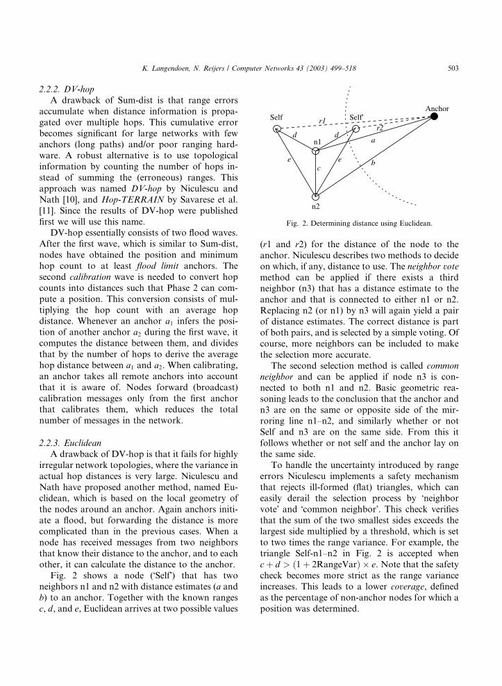
Fig. 2. Determining distance using Euclidean.


2.2.2. DV-hop

A drawback of Sum-dist is that range errors

accumulate when distance information is propa-

gated over multiple hops. This cumulative error

becomes significant for large networks with fewanchors (long paths) and/or poor ranging hard-

ware. A robust alternative is to use topological

information by counting the number of hops in-

stead of summing the (erroneous) ranges. This

approach was named DV-hop by Niculescu and

Nath [10], and Hop-TERRAIN by Savarese et al.

[11]. Since the results of DV-hop were published

first we will use this name.DV-hop essentially consists of two flood waves.

After the first wave, which is similar to Sum-dist,

nodes have obtained the position and minimum

hop count to at least flood limit anchors. The

second calibration wave is needed to convert hop

counts into distances such that Phase 2 can com-

pute a position. This conversion consists of mul-

tiplying the hop count with an average hopdistance. Whenever an anchor a1 infers the posi-

tion of another anchor a2 during the first wave, it

computes the distance between them, and divides

that by the number of hops to derive the average

hop distance between a1 and a2. When calibrating,

an anchor takes all remote anchors into account

that it is aware of. Nodes forward (broadcast)

calibration messages only from the first anchorthat calibrates them, which reduces the total

number of messages in the network.

2.2.3. Euclidean

A drawback of DV-hop is that it fails for highly

irregular network topologies, where the variance in

actual hop distances is very large. Niculescu and

Nath have proposed another method, named Eu-clidean, which is based on the local geometry of

the nodes around an anchor. Again anchors initi-

ate a flood, but forwarding the distance is more

complicated than in the previous cases. When a

node has received messages from two neighbors

that know their distance to the anchor, and to each

other, it can calculate the distance to the anchor.

Fig. 2 shows a node (�Self�) that has twoneighbors n1 and n2 with distance estimates (a andb) to an anchor. Together with the known ranges

c, d, and e, Euclidean arrives at two possible values

(r1 and r2) for the distance of the node to the

anchor. Niculescu describes two methods to decide

on which, if any, distance to use. The neighbor vote

method can be applied if there exists a thirdneighbor (n3) that has a distance estimate to the

anchor and that is connected to either n1 or n2.

Replacing n2 (or n1) by n3 will again yield a pair

of distance estimates. The correct distance is part

of both pairs, and is selected by a simple voting. Of

course, more neighbors can be included to make

the selection more accurate.

The second selection method is called common

neighbor and can be applied if node n3 is con-

nected to both n1 and n2. Basic geometric rea-

soning leads to the conclusion that the anchor and

n3 are on the same or opposite side of the mir-

roring line n1–n2, and similarly whether or not

Self and n3 are on the same side. From this it

follows whether or not self and the anchor lay on

the same side.To handle the uncertainty introduced by range

errors Niculescu implements a safety mechanism

that rejects ill-formed (flat) triangles, which can

easily derail the selection process by �neighborvote� and �common neighbor�. This check verifies

that the sum of the two smallest sides exceeds the

largest side multiplied by a threshold, which is set

to two times the range variance. For example, thetriangle Self-n1–n2 in Fig. 2 is accepted when

cþ d > ð1þ 2RangeVarÞ � e. Note that the safety

check becomes more strict as the range variance

increases. This leads to a lower coverage, defined

as the percentage of non-anchor nodes for which a

position was determined.


We now describe some modifications to Ni-

culescu�s �neighbor vote� method that remedy the

poor selection of the location for Self in important

corner cases. The first problem occurs when the

two votes are identical because, for instance, the

three neighbors (n1, n2, and n3) are collinear. Inthese cases it is hard to select the right alternative.

Our solution is to leave equal vote cases unsolved,

instead of picking an alternative and propagating

an error with 50% chance. We filter all indecisive

cases by adding the requirement that the standard

deviation of the votes for the selected distance

must be at most 1/3rd of the standard deviation of

the other distance. The second problem that weaddress is that of a bad neighbor with inaccurate

information spoiling the selection process by vot-

ing for two wrong distances. This case is filtered

out by requiring that the standard deviation of the

selected distance is at most 5% of that distance.

To achieve good coverage, we use both methods.

If both produce a result, we use the result from the

modified �neighbor vote� because we found it to bethe most accurate of the two. If both fail, the

flooding process stops leading to the situation

where certain nodes are not able to establish the

distance to enough anchor nodes. Sum-dist and

DV-hop, on the other hand, never fail to propagate

the distance and hop count, respectively.

2.3. Phase 2: Node position

In the second phase nodes determine their po-

sition based on the distance estimates to a number

of anchors provided by one of the three Phase 1

alternatives (Sum-dist, DV-hop, or Euclidean).

The Ad-hoc positioning and Robust positioning

approaches use Lateration for this purpose. N -hop

multilateration, on the other hand, uses a muchsimpler method, which we named Min–max. In

both cases the determination of the node positions

does not involve additional communication.

2.3.1. Lateration

The most common method for deriving a po-

sition is Lateration, which is a form of triangula-

tion. From the estimated distances (di) and knownpositions (xi; yi) of the anchors we derive the fol-

lowing system of equations:

ðx1 � xÞ2 þ ðy1 � yÞ2 ¼ d21 ;

..

.

ðxn � xÞ2 þ ðyn � yÞ2 ¼ d2n ;

where the unknown position is denoted by (x; y).The system can be linearized by subtracting the

last equation from the first n� 1 equations.

x21 � x2n � 2ðx1 � xnÞxþ y21 � y2n� 2ðy1 � ynÞy ¼ d2

1 � d2n ;

..

.

x2n�1 � x2n � 2ðxn�1 � xnÞxþ y2n�1

� y2n � 2ðyn�1 � ynÞy ¼ d2n�1 � d2

n :

Reordering the terms gives a proper system of

linear equations in the form Ax ¼ b, where

A ¼2ðx1 � xnÞ 2ðy1 � ynÞ

..

. ...

2ðxn�1 � xnÞ 2ðyn�1 � ynÞ

264

375;

b ¼x21 � x2n þ y21 � y2n þ d2

n � d21

..

.

x2n�1 � x2n þ y2n�1 � y2n þ d2n � d2

n�1

264

375:

The system is solved using a standard least-squares

approach: xx ¼ ðATAÞ�1 ATb. In exceptional cases

the matrix inverse cannot be computed and La-

teration fails. In the majority of the cases, how-ever, we succeed in computing a location estimate

xx. We run an additional sanity check by computing

the residue between the given distances (di) and the

distances to the location estimate xx

residue ¼Pn

i¼1

ffiffiffiffiffiffiffiffiffiffiffiffiffiffiffiffiffiffiffiffiffiffiffiffiffiffiffiffiffiffiffiffiffiffiffiffiffiffiffiffiðxi � xxÞ2 þ ðyi � yyÞ2

q� di

n:

A large residue signals an inconsistent set of

equations; we reject the location xx when the length

of the residue exceeds the radio range.

2.3.2. Min–max

Lateration is quite expensive in the number of

floating point operations that is required. A much

simpler method is presented by Savvides et al. as

part of the N -hop multilateration approach. The

Anchor1Anchor2

Anchor3

est.pos.

Fig. 3. Determining position using Min–max.


main idea is to construct a bounding box for each

anchor using its position and distance estimate,and then to determine the intersection of these

boxes. The position of the node is set to the center

of the intersection box. Fig. 3 illustrates the Min–

max method for a node with distance estimates to

three anchors. Note that the estimated position by

Min–max is close to the true position computed

through Lateration (i.e., the intersection of the

three circles).The bounding box of anchor a is created by

adding and subtracting the estimated distance (da)from the anchor position (xa, ya):

½xa � da; ya � da� � ½xa þ da; ya þ da�:The intersection of the bounding boxes is com-

puted by taking the maximum of all coordinateminimums and the minimum of all maximums:

½maxðxi � diÞ;maxðyi � diÞ�� ½minðxi þ diÞ;minðyi þ diÞ�:

The final position is set to the average of both

corner coordinates. As for Lateration, we only

accept the final position if the residue is small.

2.4. Phase 3: Refinement

The objective of the third phase is to refine the

(initial) node positions computed during Phase 2.

These positions are not very accurate, even under

good conditions (high connectivity, small range

errors), because not all available information is

used in the first two phases. In particular, most

ranges between neighboring nodes are neglected

when the node–anchor distances are determined.The iterative Refinement procedure proposed by

Savarese et al. [11] does take into account all inter-

node ranges, when nodes update their positions in

a small number of steps. At the beginning of each

step a node broadcasts its position estimate, re-

ceives the positions and corresponding range esti-

mates from its neighbors, and performs the

Lateration procedure of Phase 2 to determine itsnew position. In many cases the constraints im-

posed by the distances to the neighboring locations

will force the new position towards the true posi-

tion of the node. When, after a number of itera-

tions, the position update becomes small,

Refinement stops and reports the final position.

The basic iterative refinement procedure out-

lined above proved to be too simple to be used inpractice. The main problem is that errors propa-

gate quickly through the network; a single error

introduced by some node needs only d iterations to

affect all nodes, where d is the network diameter.

This effect was countered by (1) clipping undeter-

mined nodes with non-overlapping paths to less

than three anchors, (2) filtering out difficult sym-

metric topologies, and (3) associating a confidencemetric with each node and using them in a

weighted least-squares solution (wAx ¼ wb). The

details (see [11]) are beyond the scope of this pa-

per, but the adjustments considerably improved

the performance of the Refinement procedure.

This is largely due to the confidence metric, which

allows filtering of bad nodes, thus increasing the

(average) accuracy at the expense of coverage.The N -hop multilateration approach by Sav-

vides et al. [12] also includes an iterative refine-

ment procedure, but it is less sophisticated than

the Refinement discussed above. In particular,

they do not use weights, but simply group nodes

into so-called computation subtrees (over-con-

strained configurations) and enforce nodes within

a subtree to execute their position refinement inturn in a fixed sequence to enhance convergence to

a pre-specified tolerance. In the remainder of this


paper we will only consider the more advanced

Refinement procedure of Savarese et al.

3. Simulation environment

To compare the three original distributed lo-

calization algorithms (Ad-hoc positioning, Robust

positioning, and N -hop multilateration) and to try

out new combinations of Phases 1, 2, and 3 al-

ternatives, we extended the simulator developed by

Savarese et al. [11]. The underlying OMNeT++

discrete event simulator [17] takes care of the semi-

concurrent execution of the specific localizationalgorithm. Each sensor node �runs� the same C++

code, which is parameterized to select a particular

combination of Phases 1, 2, and 3 alternatives.

Our network layer supports localized broadcast

only, and messages are simply delivered at the

neighbors within a fixed radio range (circle) from

the sending node; a more accurate model should

take radio propagation effects into account (seefuture work). Concurrent transmissions are al-

lowed if the transmission areas (circles) do not

overlap. If a node wants to broadcast a message

while another message in its area is in progress, it

must wait until that transmission (and possibly

other queued messages) are completed. In effect we

employ a CSMA policy. Furthermore we do not

consider message corruption, so all messages sentduring our simulation are delivered (after some

delay).

At the start of a simulation experiment we

generate a random network topology according to

some parameters (#nodes, #anchors, etc.). The

nodes are randomly placed, with a uniform dis-

tribution, within a square area. Next we select

which nodes will serve as an anchor. To this endwe superimpose a grid on top of the square, and

designate to each grid point its closest node as an

anchor. The size of the grid is chosen as the

maximal number s that satisfies s� s6#anchors;

any remaining anchors are selected randomly. The

reason for carefully selecting the anchor positions

is that most localization algorithms are quite sen-

sitive to the presence, or absence, of anchors at theedges of the network. (Locating unknowns at the

edges of the network is more difficult because

nodes at the edge are less well connected and po-

sitioning techniques like Lateration perform best

when anchors surround the unknown.) Although

anchor placement may not be feasible in practice,

the majority of the nodes in large-scale networks

(1000+ nodes) will generally be surrounded byanchors. By placing anchors we can study the lo-

calization performance in large networks with

simulations involving only a modest number of

nodes.

The range between connected nodes is blurred

by drawing a random value from a normal distri-

bution having a parameterized standard deviation

and having the true range as the mean. We selectedthis error model based on the work of Whitehouse

and Culler [18], which shows that, although indi-

vidual distance measurements tend to overshoot

the real distance, a proper calibration procedure

yields distance estimates with a symmetric error

distribution. The connectivity (average number of

neighbors) is controlled by specifying the radio

range. At the end of a run the simulator outputs alarge number of statistics per node: position in-

formation, elapsed time, message counts (broken

down per type), etc. These individual node statis-

tics are combined and presented as averages (or

distributions), for example, as an average position

error. Nodes that do not produce a position are

excluded from such averaged metrics. To account

for the randomness in generating topologies andrange errors we repeated each experiment 100

times with a different seed, and report the averaged

results. To allow for easy comparison between

different scenarios, range errors as well as errors

on position estimates are normalized to the radio

range (i.e., 50% position error means a distance of

half the range of the radio between the real and

estimated positions).Standard scenario: The experiments described in

the subsequent sections share a standard scenario,

in which certain parameters are varied: radio range

(connectivity), anchor fraction, and range errors.

The standard scenario consists of a network of 225

nodes placed in a square with sides of 100 units.

The radio range is set to 14, resulting in an average

connectivity of about 12. We use an anchor frac-tion of 5%, hence, 11 anchors in total, of which 9

(3 · 3) are placed in a grid-like position. The

0.4

0.6

0.8

ance

err

oris

tanc

e]

DV-hopSum-dist

EuclideanMean

Std dev


standard deviation of the range error is set to 10%

of the radio range. The default flood limit for

Phase 1 is set to 4 (Lateration requires a minimum

of 3 anchors). Unless specified otherwise, all data

will be based on this standard scenario.

-0.4

-0.2

0

0.2

0 0.1 0.2 0.3 0.4 0.5

Rel

ativ

e di

st[x

act

ual d

Range variance

-0.4

-0.2

0

0.2

0.4

0.6

0.8

8 (4.2)

9 10 (6.4)

11 12 (9.0)

13 14 (12.1)

15 16 (15.5)

Rel

ativ

e di

stan

ce e

rror

[x a

ctua

l dis

tanc

e]

Radio range (avg. connectivity)

DV-hopSum-dist

EuclideanMean

Std dev

-0.4

-0.2

0

0.2

0.4

0.6

0.8

0 0.05 0.1 0.15 0.2

Rel

ativ

e di

stan

ce e

rror

[x a

ctua

l dis

tanc

e]

Anchor fraction

DV-hopSum-dist

EuclideanMean

Std dev

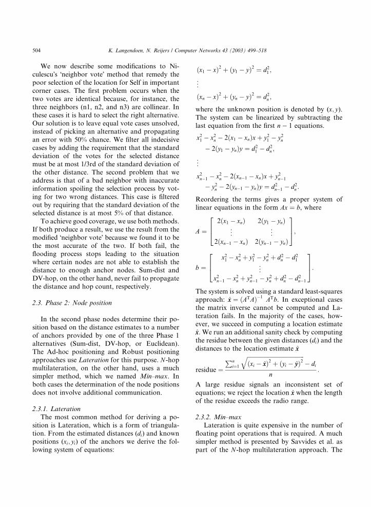
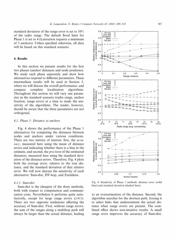
Fig. 4. Sensitivity of Phase 1 methods: distance error (solid

lines) and standard deviation (dashed lines).

4. Results

In this section we present results for the first

two phases (anchor distances and node positions).

We study each phase separately and show how

alternatives respond to different parameters. These

intermediate results will be used in Section 5,where we will discuss the overall performance, and

compare complete localization algorithms.

Throughout this section we will vary one param-

eter in the standard scenario (radio range, anchor

fraction, range error) at a time to study the sen-

sitivity of the algorithms. The reader, however,

should be aware that the three parameters are not

orthogonal.

4.1. Phase 1: Distance to anchors

Fig. 4 shows the performance of the Phase 1

alternatives for computing the distances between

nodes and anchors under various conditions.

There are two metrics of interest: first, the accu-

racy, measured here using the mean of distanceerrors and indicating whether there is a bias in the

estimate, and second, the precision of the estimated

distances, measured here using the standard devi-

ation of the distance errors. Therefore, Fig. 4 plots

both the average error, relative to the true dis-

tance, and the standard deviation of that relative

error. We will now discuss the sensitivity of each

alternative: Sum-dist, DV-hop, and Euclidean.

4.1.1. Sum-dist

Sum-dist is the cheapest of the three methods,

both with respect to computation and communi-

cation costs. Nevertheless it performs quite satis-

factorily, except for large range errors (P0.1).

There are two opposite tendencies affecting theaccuracy of Sum-dist. First, without range errors,

the sum of the ranges along a multihop path will

always be larger than the actual distance, leading

to an overestimation of the distance. Second, the

algorithm searches for the shortest path, forcing itto select links that underestimate the actual dis-

tance when range errors are present. The com-

bined effect shows non-intuitive results. A small

range error improves the accuracy of Sum-dist.

0

1

2

3

4

5

-1 -0.5 0 0.5 1

Pro

babi

lity

dens

ity

Relative range error

EuclideanOracle

Fig. 5. The impact of incorrect distance selection.


Initially, the detour effect leads to an overshoot,

but the shortest-path effect takes over when the

range errors increase, leading to a large under-

shoot.

When the radio range (connectivity) is in-

creased, more nodes can be reached in a singlehop. This leads to straighter paths (less overshoot),

and provides more options for selecting a (incor-

rect) shortest path (higher undershoot). Conse-

quently, increasing the connectivity is not

necessarily a good thing for Sum-dist.

4.1.2. DV-hop

The DV-hop method is a stable and predictablemethod. Since it does not use range measurements,

it is completely insensitive to this source of errors.

The low relative error (5%) shows that the cali-

bration wave is very effective. DV-hop searches for

the path with the minimum number of hops,

causing the average hop distance to be close to the

radio range. The last hop on the path from an

anchor to a node, however, is usually shorter thanthe radio range, which leads to a slight overesti-

mation of the node–anchor distance. This effect is

more pronounced for short paths, hence, the in-

creased error for larger radio ranges and higher

anchor fractions (i.e., fewer hops).

4.1.3. Euclidean

Euclidean is capable of determining the exactanchor–node distances, but only in the absence of

range errors and in highly connected networks.

When these conditions are relaxed, Euclidean�sperformance rapidly degrades. The curves in Fig. 4

show that Euclidean tends to underestimate the

distances. The reason is that the selection process

is forced to choose between two options that are

quite far apart and that in many cases the shortestdistance is incorrect. Consider Fig. 2 again, where

the shortest distance r2 falls within the radio range

of the anchor. If r2 would be the correct distance

then the node should be in direct contact with the

anchor avoiding the need for a selection. A similar

reasoning holds for nodes that are multiple hops

away from an anchor. Therefore nodes simply

have more chance to underestimate distances thanto overestimate them in the face of (small) range

errors.

We quantified the impact of the selection bias

towards short distances. Fig. 5 shows the distri-

bution of the errors, relative to the true distance,

on the standard scenario for Euclidean�s selectionmechanism (solid line) and an oracle that always

selects the best distance (dashed line). The oracle�sdistribution is nicely centered around zero (no er-

ror) with a sharp peak. Euclidean�s distribution, incontrast, is skewed by a heavy tail at the left, sig-

nalling a bias for underestimations.

Euclidean�s sensitivity for connectivity is not

immediately apparent from the accuracy data inFig. 4. The main effect of reducing the radio range

is that Euclidean will not be able to propagate the

anchor distances. Recall that Euclidean�s selectionmethods require at least three neighbors with a

distance estimate to advance the anchor distance

one hop. In networks with low connectivity, two

parts connected only by a few links will often not

be able to share anchors. This leads to problems inPhase 2, where fewer node positions can be com-

puted. The effects are quite pronounced, as will

become clear in Section 5 (see the coverage curves

in Fig. 10).

4.2. Phase 2: Node position

To obtain insight into the fundamental behav-ior of the the Lateration and Min–max algorithms

we now report on some experiments with con-

trolled distance errors and anchor placement. The

0

20

40

60

80

100

-0.2 -0.15 -0.1 -0.05 0 0.05 0.1 0.15 0.2

Pos

ition

err

or [

%R

]

std.dev. = 0

Bias factor

LaterationMin-max

0

20

40

60

80

100

-0.2 -0.15 -0.1 -0.05 0 0.05 0.1 0.15 0.2

Pos

ition

err

or [

%R

]

std.dev. = 0.1

Bias factor

LaterationMin-max

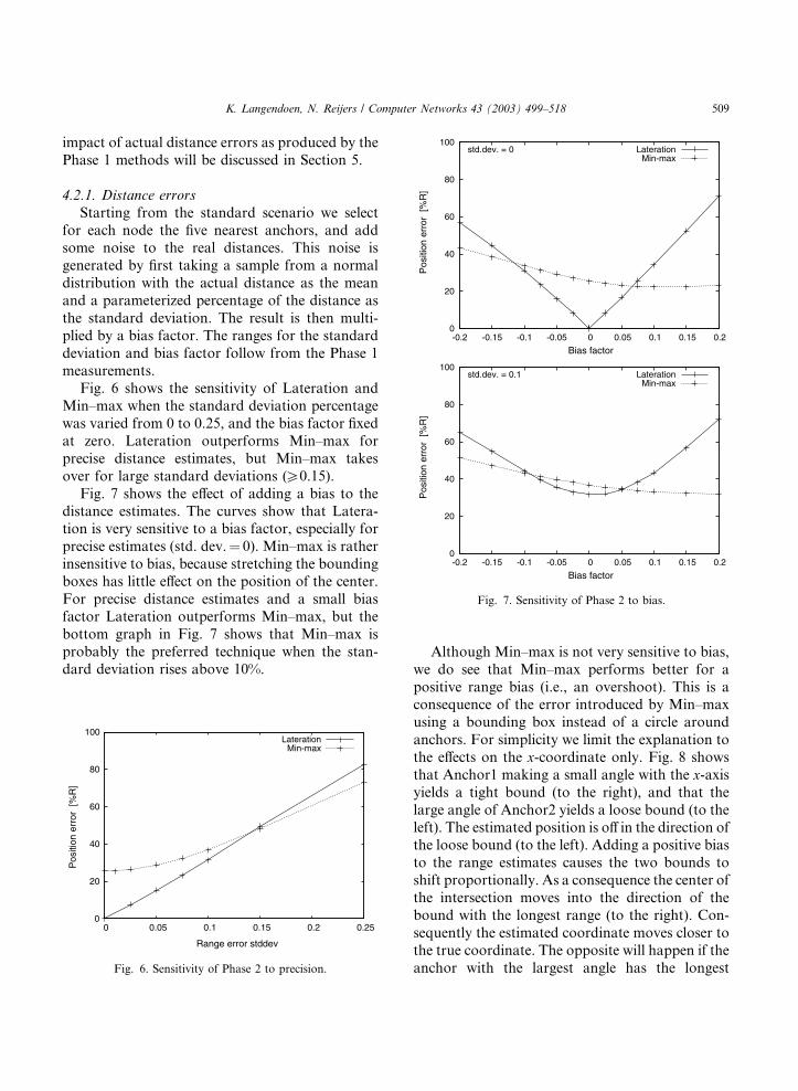
Fig. 7. Sensitivity of Phase 2 to bias.


impact of actual distance errors as produced by the

Phase 1 methods will be discussed in Section 5.

4.2.1. Distance errors

Starting from the standard scenario we select

for each node the five nearest anchors, and addsome noise to the real distances. This noise is

generated by first taking a sample from a normal

distribution with the actual distance as the mean

and a parameterized percentage of the distance as

the standard deviation. The result is then multi-

plied by a bias factor. The ranges for the standard

deviation and bias factor follow from the Phase 1

measurements.Fig. 6 shows the sensitivity of Lateration and

Min–max when the standard deviation percentage

was varied from 0 to 0.25, and the bias factor fixed

at zero. Lateration outperforms Min–max for

precise distance estimates, but Min–max takes

over for large standard deviations (P0.15).

Fig. 7 shows the effect of adding a bias to the

distance estimates. The curves show that Latera-tion is very sensitive to a bias factor, especially for

precise estimates (std. dev.¼ 0). Min–max is rather

insensitive to bias, because stretching the bounding

boxes has little effect on the position of the center.

For precise distance estimates and a small bias

factor Lateration outperforms Min–max, but the

bottom graph in Fig. 7 shows that Min–max is

probably the preferred technique when the stan-dard deviation rises above 10%.

0

20

40

60

80

100

0 0.05 0.1 0.15 0.2 0.25

Pos

ition

err

or [

%R

]

Range error stddev

LaterationMin-max

Fig. 6. Sensitivity of Phase 2 to precision.

Although Min–max is not very sensitive to bias,

we do see that Min–max performs better for a

positive range bias (i.e., an overshoot). This is aconsequence of the error introduced by Min–max

using a bounding box instead of a circle around

anchors. For simplicity we limit the explanation to

the effects on the x-coordinate only. Fig. 8 shows

that Anchor1 making a small angle with the x-axisyields a tight bound (to the right), and that the

large angle of Anchor2 yields a loose bound (to the

left). The estimated position is off in the direction ofthe loose bound (to the left). Adding a positive bias

to the range estimates causes the two bounds to

shift proportionally. As a consequence the center of

the intersection moves into the direction of the

bound with the longest range (to the right). Con-

sequently the estimated coordinate moves closer to

the true coordinate. The opposite will happen if the

anchor with the largest angle has the longest

Anchor1

Anchor2

r1α1

r2α2

Fig. 8. Min–max scenario.


distance. Min–max selects the strongest bounds,

leading to a preference for small angles and small

distances, which favors the number of ‘‘good’’

cases where the coordinate moves closer to the true

coordinate if a positive range bias is added.

4.2.2. Anchor placement

Min–max has the advantage of being compu-

tationally cheap and insensitive to errors, but it

requires a good constellation of anchors; in par-

ticular, Savvides et al. recommend placing the

anchors at the edges of the network [12]. If the

anchors cannot be placed and are uniformly dis-

tributed across the network, the accuracy of thenode positions at the edges is rather poor. Fig. 9

illustrates this problem graphically. We applied

Min–max and Lateration to the example network

presented in Fig. 1. In the case of Min–max, all

nodes that lie outside the convex envelope of the

Min-max

AnchorUnknown

Estimated positio

Fig. 9. Node locations computed fo

four anchor nodes are drawn inwards, yielding

considerable errors (indicated by the dashed lines);

the nodes within the envelope are located ade-

quately. Lateration, on the other hand, performs

much better. Nodes at the edges are located less

accurately than interior nodes, but the magnitudeof and variance in the errors is smaller than for

Min–max.

The differences in accuracy between Lateration

and Min–max can be considerable. For instance,

when DV-hop in combination with Min–max is

run on the standard scenario (with grid-based

anchors), the average position accuracy degrades

from 43% to 77% when anchors are randomlydistributed. The accuracy of Lateration also de-

grades, but only from 42% to 54%.

5. Discussion

Now that we know the behavior of the indi-

vidual Phases 1 and 2 components, we can turn tothe performance effects of concatenating both

phases, followed by applying Refinement in Phase

3. We will study the sensitivity of various combi-

nations to connectivity, anchor fraction, and range

errors using both the resulting position error and

coverage.

5.1. Phases 1 and 2 combined

Combining the three Phase 1 alternatives (Sum-

dist, DV-hop, and Euclidean) with the two Phase 2

n

Lateration

r network topology of Fig. 1.

0

20

40

60

80

100

0 0.1 0.2 0.3 0.4 0.5

Cov

erag

e [%

]

Range variance

DV-hopSum-dist

EuclideanLateration

Min-max

0

20

40

60

80

100

8 (4.2)

9 10 (6.4)

11 12 (9.0)

13 14 (12.1)

15 16 (15.5)

Cov

erag

e [%

]


DV-hopSum-dist

EuclideanLateration

Min-max

0

20

40

60

80

100

0 0.05 0.1 0.15 0.2

Cov

erag

e [%

]

Anchor fraction

DV-hopSum-dist

EuclideanLateration

Min-max

Fig. 10. Coverage of Phase 1/2 combinations.

0

50

100

150

0 0.1 0.2 0.3 0.4 0.5

Pos

ition

err

or [

%R

]

Range variance

DV-hopSum-dist

EuclideanLateration

Min-max

0

50

100

150

200

250

300

8 (4.2)

9 10 (6.4)

11 12 (9.0)

13 14 (12.1)

15 16 (15.5)

Pos

ition

err

or [

%R

]


DV-hopSum-dist

EuclideanLateration

Min-max

0

50

100

150

0 0.05 0.1 0.15 0.2

Pos

ition

err

or [

%R

]

Anchor fraction

DV-hopSum-dist

EuclideanLateration

Min-max

Fig. 11. Accuracy of Phase 1/2 combinations.


alternatives (Lateration and Min–max) yields atotal of six possibilities. We will analyze the dif-

ferences in terms of coverage (Fig. 10) and position

accuracy (Fig. 11). When fine-tuning localization

algorithms, the trade-off between accuracy and

coverage plays an important role; dropping diffi-

cult cases increases average accuracy at the ex-

pense of coverage.

5.1.1. Coverage

Fig. 10 shows the coverage of the six Phase 1/

Phase 2 combinations for varying range error


(top), radio range (middle), and anchor fraction

(bottom). The solid lines denote the Lateration

variants; the dashed lines denote the Min–max

variants. The first observation is that Sum-dist and

DV-hop are able to determine the range to enough

anchors to position all the nodes, except in caseswhen the radio range is small (611), or equiva-

lently when the connectivity is low (67.5). In such

sparse networks, Lateration provides a slightly

higher coverage than Min–max. This is caused by

the sanity check on the residue. A consistent set of

anchor positions and distance estimates leads to a

low residue, but the reverse does not hold. Occa-

sionally if Lateration is used with an inconsistentset, an outlier is produced with a small residue,

which is accepted. Min–max does not suffer from

this problem because the positions are always

constrained by the bounding boxes and thus can-

not produce such outliers. Lateration�s higher

coverage results in higher errors, see the accuracy

curves in Fig. 11.

The second observation is that Euclidean hasgreat difficulty in achieving a reasonable coverage

when conditions are non-ideal. The combination

with Min–max gives the highest coverage, but even

that combination only achieves acceptable results

under ideal conditions (range variance 6 0.1,

connectivity P15, anchor fraction P0.1). The

reason for Euclidean�s poor coverage is twofold.

First, the triangles used to propagate anchor dis-tances are checked for validity (see Section 2.2.3);

this constraint becomes more strict as the range

variance increases, hence the significant drop in

coverage. Second, Euclidean can only forward

anchor distances if enough neighbors are present

(see Section 4.1.3) resulting in many nodes ‘‘lo-

cating’’ only one or two anchors. Lateration re-

quires at least three anchors, but Min–max doesnot have this requirement. This explains why the

Euclidean/Min–max combination yields a higher

coverage. Again, the price is paid in terms of ac-

curacy (cf. Fig. 11).

5.1.2. Accuracy

Fig. 11 gives the average position error of the

six combinations under the same varying condi-tions as for the coverage plots. To ease the inter-

pretation of the accuracies we filtered out

anomalous cases whose coverage is below 50%,

which mainly concerns Euclidean�s results. The

most striking observation is that the Euclidean/

Lateration combination clearly outperforms the

others in the absence of range errors: 0% error

versus at least 29% (Sum-dist/Min–max). Thisfollows from the good performance of both Eu-

clidean and Lateration in this case (see Section 4).

The downside is that both components were also

shown to be very sensitive to range errors. Con-

sequently, the average position error increases

rapidly if noise is added to the range estimates; at

just 2% range variance, Euclidean/Lateration

looses its advantage over the Sum-dist/Min–maxcombination. When the range variance exceeds

10%, DV-hop performs best. In this scenario DV-

hop achieves comparable accuracies for both La-

teration and Min–max. Which Phase 2 algorithm

is most appropriate depends on anchor placement,

and whether the higher computation cost of La-

teration is important.

Notice that Sum-dist/Lateration actually be-comes more accurate when a small amount of

range variance is introduced, while the errors of

Sum-dist/Min–max increase. This matches the re-

sults found in sections 4.1.1 and 4.2.1. Adding a

small range error causes Sum-dist to yield more

accurate distance estimates (cf. Fig. 4). Lateration

benefits greatly from a reduced bias, but Min–max

is not that sensitive and even deteriorates slightly(cf. Fig. 7). The combined effect is that Sum-dist/

Lateration benefits from small range errors; Sum-

dist/Min–max does not show this unexpected be-

havior.

All six combinations are quite sensitive to

the radio range (connectivity). A minimum

connectivity of 9.0 is required (at radio range

12) for DV-hop and Sum-dist, in which caseSum-dist slightly outperforms DV-hop and the

difference between Lateration and Min–max is

negligible. Euclidean does not perform well

because of the 10% range variance in the

standard scenario.

The sensitivity to the anchor fraction is quite

similar for all combinations. More anchors ease

the localization task, especially for Euclidean, butthere is no hard threshold like for the sensitivity to

connectivity.


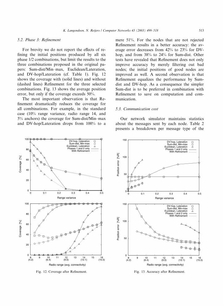
5.2. Phase 3: Refinement

For brevity we do not report the effects of re-

fining the initial positions produced by all six

phase 1/2 combinations, but limit the results to thethree combinations proposed in the original pa-

pers: Sum-dist/Min–max, Euclidean/Lateration,

and DV-hop/Lateration (cf. Table 1). Fig. 12

shows the coverage with (solid lines) and without

(dashed lines) Refinement for the three selected

combinations. Fig. 13 shows the average position

error, but only if the coverage exceeds 50%.

The most important observation is that Re-finement dramatically reduces the coverage for

all combinations. For example, in the standard

case (10% range variance, radio range 14, and

5% anchors) the coverage for Sum-dist/Min–max

and DV-hop/Lateration drops from 100% to a

0

20

40

60

80

100

0 0.1 0.2 0.3 0.4 0.5

Cov

erag

e [%

]

Range variance

DV-hop, LaterationSum-dist, Min-max

Euclidean, LaterationPhases 1 and 2 only

With Refinement

0

20

40

60

80

100

8 (4.2)

9 10 (6.4)

11 12 (9.0)

13 14 (12.1)

15 16 (15.5)

Cov

erag

e [%

]


Fig. 12. Coverage after Refinement.

mere 51%. For the nodes that are not rejected

Refinement results in a better accuracy: the av-

erage error decreases from 42% to 23% for DV-

hop, and from 38% to 24% for Sum-dist. Other

tests have revealed that Refinement does not only

improve accuracy by merely filtering out badnodes; the initial positions of good nodes are

improved as well. A second observation is that

Refinement equalizes the performance by Sum-

dist and DV-hop. As a consequence the simpler

Sum-dist is to be preferred in combination with

Refinement to save on computation and com-

munication.

5.3. Communication cost

Our network simulator maintains statistics

about the messages sent by each node. Table 2

presents a breakdown per message type of the

0

50

100

150

0 0.1 0.2 0.3 0.4 0.5

Pos

ition

err

or [

%R

]

Range variance



With Refinement

0

50

100

150

8 (4.2)

9 10 (6.4)

11 12 (9.0)

13 14 (12.1)

15 16 (15.5)

Pos

ition

err

or [

%R

]




With Refinement

Fig. 13. Accuracy after Refinement.

Table 2

Average number of messages per node

Type Sum-dist DV-hop Euclidean

Flood 4.3 2.2 3.5

Calibration – 2.6 –

Refinement 32 29 20


three original localization combinations (with

Refinement) on the standard scenario.The number of messages in Phase 1 (Flood+

Calibration) is directly controlled by the flood limit

parameter, which is set to 4 by default. Fig. 14

shows the message counts in Phase 1 for various

flood limits. Note that Sum-dist and DV-hop scale

almost linearly; they level off slightly because in-

formation on multiple anchors can be combined in

a single message. Euclidean, on the other hand,levels off completely because of the difficulties in

propagating anchor distances, especially along

long paths.

For Sum-dist and DV-hop we expect nodes to

transmit a message per anchor. Note, however,

that for low flood limits the message count is

higher than expected. In the case of DV-hop, the

count also includes the calibration messages. Withsome fine-tuning the number of calibration mes-

sages can be limited to one, but the current im-

plementation needs about as many messages as the

flooding itself. A second factor that increases the

number of messages for DV-hop and Sum-dist is

the update information to be sent when a shorter

path is detected, which happens quite frequently

for Sum-dist. Finally, all three algorithms are self-organizing and nodes send an extra message when

discovering a new neighbor that needs to be in-

formed of the current status.

Although the flood limit is essential for crafting

scalable algorithms, it affects the accuracy; see the

bottom graph in Fig. 14. Note that using a higher

flood limit does not always improve accuracy. In

the case of Sum-dist, there is a trade-off betweenusing few anchors with accurate distance infor-

mation, and using many anchors with less accurate

information. With DV-hop, on the other hand, the

distance estimates become more accurate for

longer paths (last-hop effect, see Section 4.1.2).

Euclidean�s error only increases with higher flood

limits because it starts with a low coverage, which

also increases with higher flood limits. DV-hop

and Sum-dist reach almost 100% coverage at flood

limits of 2 (Min–max) or 3 (Lateration).

With the flood limit set to 4, the nodes send

about four messages during Phase 1 (cf. Table 2).This is comparable to the three messages needed

by a centralized algorithm: set up a spanning tree,

collect range information, and distribute node

positions. Running Refinement in Phase 3, on the

other hand, is extremely expensive, requiring 20

(Euclidean) to 32 messages (Sum-dist). The prob-

lem is that Refinement takes many iterations be-

fore local convergence criteria decide to terminate.We added a limit to the number of Refinement

messages a node is allowed to send. The effect of

this is shown in Fig. 15. A Refinement limit of 0

means that no refinement messages are sent, and

Refinement is skipped completely.

The position errors in Fig. 15 show that most of

the effect of Refinement takes place in the first few

iterations, so hard limiting the iteration count is avalid option. For example, the accuracy obtained

by DV-hop without Refinement is 42% and it

drops to 28% after two iterations; an additional

4% drop can be achieved by waiting until Refine-

ment terminates based on the local stopping cri-

teria, but this requires another 27 messages (29 in

total). Thus the communication cost of Refine-

ment can effectively be reduced to less than thecosts for Phase 1. Nevertheless, the poor coverage

of Refinement limits its practical use.

5.4. Recommendations

From the previous discussion it follows that no

single combination of Phases 1, 2, and 3 alterna-

tives performs best under all conditions; each

combination has its strengths and weaknesses. The

results presented in Section 5 follow from chang-

ing one parameter (radio range, range variance,

and anchor fraction) at a time. Since the sensitivityof the localization algorithms may not be orthog-

onal in the three parameters, it is difficult to derive

general recommendations. Therefore, we con-

ducted an exhaustive search for the best algorithm

in the three-dimensional parameter space. For

readability we do not present the raw outcome, a

0

20

40

60

80

100

0 2 4 6 8 10

Cov

erag

e [%

]

Refinement limit

DV-hop, Lateration, RefinementSum-dist, Min-max, Refinement

Euclidean, Lateration, Refinement

0

20

40

60

80

100

0 2 4 6 8 10

Pos

ition

err

or [

%R

]

Refinement limit

DV-Hop, Lateration, RefinementSum-dist, Min-max, Refinement

Euclidean, Lateration, Refinement

Fig. 15. Effect of Refinement limit.

0

1

2

3

4

5

6

7

8

0 2 4 6 8 10

#Mes

sage

s pe

r no

de

Flood limit


Euclidean, Lateration

0

50

100

150

0 2 4 6 8 10

Pos

ition

err

or [

%R

]

Flood limit


Euclidean, Lateration

Fig. 14. Sensitivity to flood limit.


6 · 6 · 5 cube, but show a two-dimensional slice

instead. We found that the localization algorithms

are the least sensitive to the anchor fraction, so

Table 3 presents the results of varying the radio

range and the range variance, while keeping the

anchor fraction fixed at 5%. In each case we listthe algorithm that achieves the best accuracy (i.e.,

the lowest average position error) under the con-

dition that its coverage exceeds 50%. Since Re-

finement often results in very poor coverage, we

only examine Phases 1 and 2 here.

The exhaustive parameter search, and basic

observations about Refinement, lead to the fol-

lowing recommendations:

• Euclidean should always be used in combination

with Lateration, but only if distances can be

measured very accurately (range variance

<2%) and the network has a high connectivity

(P12). When the anchor fraction is increased,

Euclidean captures some more entries in the

left-upper corner of Table 3, and the conditions

on range variance and connectivity can be re-

laxed slightly. Nevertheless, the window of op-

portunity for Euclidean/Lateration is rathersmall.

• DV-hop should be used when there are no or

poor distance estimates, for example, those ob-

tained from the signal strength (cf. the bottom

rows in Table 3). Our results show that DV-

hop outperforms the other methods when the

range variance is large (>10% in this slice).

The presence of Lateration in the last column,that is, with a very low connectivity, is an arti-

fact caused by the filtering on coverage. DV-

hop/Min–max has a coverage of 49% in this

case (versus 56% for DV-hop/Lateration), but

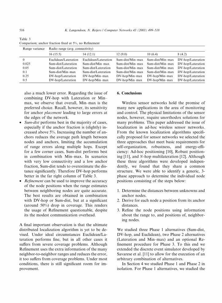
Table 3

Comparison; anchor fraction fixed at 5%, no Refinement

Range variance Radio range (avg. connectivity)

16 (15.5) 14 (12.1) 12 (9.0) 10 (6.4) 8 (4.2)

0 Euclidean/Lateration Euclidean/Lateration Sum-dist/Min–max Sum-dist/Min–max DV-hop/Lateration

0.025 Sum-dist/Lateration Sum-dist/Min–max Sum-dist/Min–max Sum-dist/Min–max DV-hop/Lateration

0.05 Sum-dist/Lateration Sum-dist/Lateration Sum-dist/Min–max Sum-dist/Min–max DV-hop/Lateration

0.1 Sum-dist/Min–max Sum-dist/Lateration Sum-dist/Min–max Sum-dist/Min–max DV-hop/Lateration

0.25 DV-hop/Lateration DV-hop/Min–max DV-hop/Min–max DV-hop/Min–max DV-hop/Lateration

0.5 DV-hop/Lateration DV-hop/Min–max DV-hop/Min–max DV-hop/Min–max DV-hop/Lateration


also a much lower error. Regarding the issue of

combining DV-hop with Lateration or Min–

max, we observe that overall, Min–max is the

preferred choice. Recall, however, its sensitivity

for anchor placement leading to large errors at

the edges of the network.

• Sum-dist performs best in the majority of cases,

especially if the anchor fraction is (slightly) in-creased above 5%. Increasing the number of an-

chors reduces the average path length between

nodes and anchors, limiting the accumulation

of range errors along multiple hops. Except

for a few corner cases, Sum-dist performs best

in combination with Min–max. In scenarios

with very low connectivity and a low anchor

fraction, Sum-dist tends to overestimate the dis-tance significantly. Therefore DV-hop performs

better in the far right column of Table 3.

• Refinement can be used to improve the accuracy

of the node positions when the range estimates

between neighboring nodes are quite accurate.

The best results are obtained in combination

with DV-hop or Sum-dist, but at a significant

(around 50%) drop in coverage. This rendersthe usage of Refinement questionable, despite

its the modest communication overhead.

A final important observation is that the ultimate

distributed localization algorithm is yet to be de-

vised. Under ideal circumstances Euclidean/La-

teration performs fine, but in all other cases it

suffers from severe coverage problems. AlthoughRefinement uses the extra information of the many

neighbor-to-neighbor ranges and reduces the error,

it too suffers from coverage problems. Under most

conditions, there is still significant room for im-

provement.

6. Conclusions

Wireless sensor networks hold the promise of

many new applications in the area of monitoring

and control. The physical limitations of the sensor

nodes, however, require unorthodox solutions for

many problems. This paper addressed the issue of

localization in ad-hoc wireless sensor networks.From the known localization algorithms specifi-

cally proposed for sensor networks we selected the

three approaches that meet basic requirements for

self-organization, robustness, and energy-effi-

ciency: Ad-hoc positioning [10], Robust position-

ing [11], and N -hop multilateration [12]. Although

these three algorithms were developed indepen-

dently, we found that they share a commonstructure. We were able to identify a generic, 3-

phase approach to determine the individual node

positions consisting of the steps below:

1. Determine the distances between unknowns and

anchor nodes.

2. Derive for each node a position from its anchor

distances.3. Refine the node positions using information

about the range to, and positions of, neighbor-

ing nodes.

We studied three Phase 1 alternatives (Sum-dist,

DV-hop, and Euclidean), two Phase 2 alternatives

(Lateration and Min–max) and an optional Re-

finement procedure for Phase 3. To this end weextended the discrete event simulator developed by

Savarese et al. [11] to allow for the execution of an

arbitrary combination of alternatives.

In Section 4 we studied Phase 1 and Phase 2 in

isolation. For Phase 1 alternatives, we studied the


sensitivity to range errors, connectivity, and frac-

tion of anchor nodes (with known positions). DV-

hop proved to be stable and predictable, Sum-dist

and Euclidean showed tendencies to under esti-

mate the distances between anchors and un-

knowns. Euclidean was found to have difficultiesin propagating distance information under non-

ideal conditions, leading to low coverage in the

majority of cases. The results for Phase 2 showed

that Lateration is capable of obtaining very accu-

rate positions, but also that it is very sensitive to

the accuracy and precision of the distance esti-

mates. Min–max is more robust, but is sensitive to

the placement of anchors, especially at the edges ofthe network.

In Section 5 we compared all six phase 1/2

combinations under different conditions. We

found that no single combination performs best;

which algorithm is to be preferred depends on the

conditions (range errors, connectivity, anchor

fraction and placement). The Euclidean/Lateration

combination [10] should be used only in the ab-sence of range errors (variance <2%) and requires

a high node connectivity. The DV-hop/Min–max

combination, which is a minor variation on the

DV-hop/Lateration approach proposed in [10,11],

performs best when there are no or poor distance

estimates, for example, those obtained from the

signal strength. The Sum-dist/Min–max combina-

tion [12] is to be preferred in the majority of otherconditions. The benefit of running Refinement in

Phase 3 is considered to be questionable since in

many cases the coverage dropped by 50%, while

the accuracy only improved significantly in the

case of small range errors. The communication

overhead of Refinement was shown to be modest

(two messages per node) in comparison to the

controlled flooding of Phase 1 (four messages pernode).

Future work: Regarding the future, we observed

that the ultimate distributed localization algorithm

is yet to be devised. Under ideal circumstances

Euclidean/Lateration performs fine, but in all

other cases there is significant room for improve-

ment. Furthermore, additional effort is needed to

bridge the gap between simulations and real-worldlocalization systems. For instance, we need to

gather more data on the actual behavior of sensor

nodes, particularly with respect to physical effects

like multipath, interference, and obstruction.

Acknowledgements

We thank Andreas Savvides and Dragos

Niculescu for sharing their code with us and

commenting on the draft version of this paper. We

also thank the anonymous reviewers for their

comments and suggestions to improve the quality

of this paper.

References

[1] I. Akyildiz, W. Su, Y. Sankarasubramaniam, E. Cayirci, A

survey on sensor networks, IEEE Commun. Mag. 40 (8)

(2002) 102–114.

[2] S. Atiya, G. Hager, Real-time vision-based robot localiza-

tion, IEEE Trans. Robot. Automat. 9 (6) (1993) 785–800.

[3] J. Leonard, H. Durrant-Whyte, Mobile robot localization

by tracking geometric beacons, IEEE Trans. Robot.

Automat. 7 (3) (1991) 376–382.

[4] R. Tinos, L. Navarro-Serment, C. Paredis, Fault tolerant

localization for teams of distributed robots, in: IEEE

International Conference on Intelligent Robots and Sys-

tems, vol. 2, Maui, HI, 2001, pp. 1061–1066.

[5] J. Hightower, G. Bordello, Location systems for ubiqui-

tous computing, IEEE Comp. 34 (8) (2001) 57–66.

[6] N. Bulusu, J. Heidemann, D. Estrin, GPS-less low-cost

outdoor localization for very small devices, IEEE Person.

Commun. 7 (5) (2000) 28–34.

[7] S. Capkun, M. Hamdi, J.-P. Hubaux, GPS-free positioning

in mobile ad-hoc networks, Cluster Comput. 5 (2) (2002)

157–167.

[8] J. Chen, K. Yao, R. Hudson, Source localization and

beamforming, IEEE Signal Process. Mag. 19 (2) (2002) 30–

39.

[9] L. Doherty, K. Pister, L.E. Ghaoui, Convex position

estimation in wireless sensor networks, in: IEEE Infocom

2001, Anchorage, AK, 2001.

[10] D. Niculescu, B. Nath, Ad-hoc positioning system, in:

IEEE GlobeCom, 2001.

[11] C. Savarese, K. Langendoen, J. Rabaey, Robust position-

ing algorithms for distributed ad-hoc wireless sensor

networks, in: USENIX Technical Annual Conference,

Monterey, CA, 2002, pp. 317–328.

[12] A. Savvides, H. Park, M. Srivastava, The bits and flops of

the N -hop multilateration primitive for node localization

problems, in: First ACM International Workshop on

Wireless Sensor Networks and Application (WSNA),

Atlanta, GA, 2002, pp. 112–121.

[13] N. Priyantha, A. Chakraborty, H. Balakrishnan,

The Cricket location-support system, in: 6th ACM


International Conference on Mobile Computing and

Networking (Mobicom), Boston, MA, 2000, pp. 32–

43.

[14] J. Hightower, R. Want, G. Borriello, SpotON: An indoor

3D location sensing technology based on RF signal

strength, UW CSE 00-02-02, University of Washington,

Department of Computer Science and Engineering, Seattle,

WA, February 2000.

[15] L. Girod, D. Estrin, Robust range estimation using

acoustic and multimodal sensing, in: IEEE/RSJ Interna-

tional Conference on Intelligent Robots and Systems

(IROS), Maui, Hawaii, 2001.

[16] Y. Xu, J. Heidemann, D. Estrin, Geography-informed

energy conservation for ad-hoc routing, in: 7th ACM

International Conference on Mobile Computing and Net-

working (Mobicom), Rome, Italy, 2001, pp. 70–84.

[17] A. Varga, The OMNeT++ discrete event simulation

system, in: European Simulation Multiconference

(ESM�2001), Prague, Czech Republic, 2001.

[18] K. Whitehouse, D. Culler, Calibration as parameter

estimation in sensor networks, in: First ACM International

Workshop on Wireless Sensor Networks and Application

(WSNA), Atlanta, GA, 2002, pp. 59–67.

Koen Langendoen is currently an as-sistant professor at the faculty of In-formation Technology and Systems,Delft University of Technology, TheNetherlands. He earned an M.Sc. inComputer Science from the VrijeUniversiteit in 1988 and a Ph.D. inComputer Science from the Universi-teit van Amsterdam in 1993. His re-search interests include systemsoftware for parallel processing, wear-able computing, embedded systems,and wireless sensor networks.

Niels Reijers received the M.Sc. degreein Computer Science from Delft Uni-versity of Technology, The Nether-lands, in 2002. He is currently workingtowards a doctoral degree at the sameuniversity in the area of wireless sensornetworks. Within the Consensus pro-ject his task is to develop energy-effi-cient collaboration services that willsupport self-organizing networks ofsensor nodes.

Documents

Distributed localization in wireless sensor networks: a ...koen/papers/compnw.pdf · Distributed localization in wireless sensor networks: a quantitative comparison Koen Langendoen