DISTRIBUTED ENERGY RESOURCE ALLOCATION … AN ECONOMIC AND TECHNOLOGICAL ... Distributed Energy Resource Allocation and Dispatch 183 ... reference for the marginal power plant

182 International Journal of Electronic Business Management, Vol. 5, No. 3, pp. 182-196 (2007)

DISTRIBUTED ENERGY RESOURCE ALLOCATION AND

DISPATCH: AN ECONOMIC AND TECHNOLOGICAL

PERCEPTION

Michael Stadler1*, Friederich Kupzog2 and Peter Palensky2 1Electricity Markets and Policy Group

Berkeley (CA 94720), USA 2Institute of Computer Technology

Vienna University of Technology

Gusshausstrasse 27-29/384, A-1040 Vienna, Austria

ABSTRACT

Despite the recent easing of electricity wholesale prices, the absolute level of on-peak

electricity prices for most markets is tremendously high. The German on-peak electricity

wholesale price is about 290% higher than six years ago, which has resulted in tariff hikes.

These tariff hikes burden economies worldwide and result in higher inflation or economic

cool down. The first part of this paper focuses on market power and the amplified price

spikes during on-peak hours especially. A simple model is presented that is able to describe

the strategic behaviour of similar market players during on-peak and off-peak hours.

Furthermore, the work shows in an easy way how consumers can mitigate market power by

creating a short-term demand curve due to load-management programs. We conclude that

for a sustainable electricity system without unusually high price spikes, a consideration of

the short-term demand curve by using automated systems is important. It is necessary to

introduce a technical infrastructure that makes unused load shift potential accessible and

gives consumers the possibility to respond to price spikes easily in the short term without

sacrificing comfort or services. We present a new automated approach to create such a

short-term demand curve. The proposed Integral Resource Optimization Network (IRON)

indicates a robust and distributed automation network for the optimization of distributed

energy supply and usage. We describe a basic generic model for load shifting, which allows

describing a collective storage management in an easy way. Furthermore, the first real

implementation result of the research is presented–the so-called IRON-Box, a hardware

interface that realises the interface between load resources and the IT infrastructure.

Keywords: Demand Response, Distributed Generation (DG), Information Systems, Load

Management, Market Issues and Strategic Pricing, Market Power, Real-Time-Pricing

* Corresponding author: [email protected] or [email protected]

1. INTRODUCTION

Energy consumers worldwide have been

concerned for the past three years about dramatically

increasing energy prices. Before electricity market

restructuring in Europe, politicians always

emphasized the advantages of liberalization. A very

important objective was to provide “cheap” electricity

for the European Union and its economy. Now, it

looks like the exact opposite happened (see also [7])

Within the last six years, the average electricity

wholesale prices in Germany and Austria increased

by 285%. The average off-peak prices for the

German/Austrian market increased by 270%

compared to an increase of 290% for the average

on-peak prices. On-peak prices are increasing faster

than the off-peak prices, which indicates market

problems especially during on-peak hours. Empirical

investigations of several other spot markets show the

same pattern. For example the Nord Pool system

price shows average on-peak spikes in the 80€/MWh

range. Furthermore, the investigations show that

many markets get more and more volatile, which

increases the uncertainties for market participants

(see also [2]). These higher prices on the wholesale

markets translate into higher consumer prices (see

also [7]). Within the last six years, the average

electricity price (including taxes) for industrial

consumers in the European Union increased by 31%

M. Stadler et al.: Distributed Energy Resource Allocation and Dispatch 183

(source: [7]), which burdens the European economy

considerably.

Furthermore, these price jumps are not only in

the electricity sector, but also in the natural gas sector.

Natural gas and oil are used as energy inputs in many

electric power plants worldwide, and therefore, the

jump in primary energy explains partly the

skyrocketing electricity prices. Additionally, the new

CO2 emissions trading system may contribute partly

to these higher prices. However, the question is: is it

possible that the missing short-term demand curve

contributes to the tight volatile market and high prices

we see now?

Of course, we might run out of oil and peak in

the production very soon, but in the short to mid term

the problem certainly does not lie in the problem of

peak oil, directly. The problem is constituted by the

fact that consumers have no or only limited capability

to react to price signals during times with limited

supply capacities and high demand. For example, if

you live in the outskirts of Los Angeles and you have

to get to the city for work, the only possibility you

have is to drive. This means your response to high

gasoline prices will be almost zero, but this behaviour

creates economic inefficiency for the whole society.

In the electricity sector, we have similar

conditions. Which consumer in the European Union

can respond to real-time prices and change his / her

consumption behaviour? Almost no short-term elastic

demand curve exists in most of the electricity

markets. This problem is basically constituted by the

fact that no information flows between suppliers and

consumers (in terms of real-time price signals): the

market is in an unstable diverging condition.

On the other hand, research reveals that it

would be possible to shed peak demand with

enhanced automation technologies without loss in

comfort. Such systems can create elastic demand

curves in a simple way. [3] shows the Albertson

enhanced lighting control system, which allows 300

Albertson stores to reduce peak demand up to 7.5

MW. For more information on large facilities and

demand-response please refer to [11].

In this work, we present a new approach to

create a long- and short-term demand curve that

stabilizes the electricity market, which then

contributes to CO2 emissions reduction. The proposed

Integral Resource Optimization Network (IRON)

indicates a robust and distributed automation network

for the optimization of distributed energy supply and

usage. Networked consumers, producers, and storage

services (e.g. refrigerators) have the (technical)

capability and the right to manage – within certain

limits – their supply and consumption over time. This

pattern will enable previously unused and

inaccessible shiftable potentials and directly result in

a long- and short-term elastic demand curve that

contributes to sustainable energy market equilibria.

2. THE THREAT OF AMPLIFIED

PRICE SPIKES

Figure 1 shows for the German / Austrian

electricity market an average daily wholesale price

pattern. The figure denotes the disproportionate

increase in on-peak2 prices compared to off-peak

prices.

0

50

100

150

200

250

300

350

1 2 3 4 5 6 7 8 9 10 11 12 13 14 15 16 17 18 19 20 21 22 23 24

hours€

/MW

h July 2006

July 2003

max. ∆on-peak

max. ∆off-peak

Figure 1: Average German/Austrian daily wholesale

prices for selected months. Source: Own database.

The missing possibility of consumers to

respond to price signals may provoke the threat of

strategic on-peak pricing. The natural gas price – as

reference for the marginal power plant - increased by

167% from July 2003 to July 2006, but the average

on-peak price increased by 269% in the same period,

and therefore, we focus on the threat of amplified

price spikes due to market power3. To demonstrate

this behaviour we will show a simple gaming

approach for the Nordic Power market. Additional

information according market power in the Nordic

power market and German market can be found at [5]

and [10]. The theory is based on the assumption that

some companies monitor the market conditions and

withdraw one or more power plant units to shift the

supply curve (see Figure 2) to the left. In this way the

intersection between supply and demand can be

modified. The suppliers try to control the market

price due to faked maintenance. During off-peak

conditions, the withdrawal of some power plant units

2 In practice the definition of on-peak and off-peak depends on the country considered. On-Peak: 08.00 hours to 20.00 hours for Germany and Austria. 3 We do not postulate that strategic pricing is the one and only reason for these high prices. Other reasons for the disproportional increase can be the CO2 emissions trading system, different input fuels during on-peak hours as well as lower power plant efficiencies during on-peak hours. We do not investigate the impact of the CO2 emissions trading system, different input fuels or lower power plant efficiencies in this work.

International Journal of Electronic Business Management, Vol. 5, No. 3 (2007)

184

will not change much. The marginal4 power plant

remains constant, and therefore, no market price

change can be created5. However, if market players

realize that the market is in an on-peak condition and

about to use the next type of power plant very soon,

the players can provoke a jump to the next marginal

power plant (e.g. 62 GW on-peak demand according

Figure 2 and Table 1).

Figure 2: Modified winter supply curve for the

Nordic6 power market, 60 per cent water reservoirs

(Supply curve based on installed capacity in 2000 and

price data for 2000). Source: [17].

During on-peak conditions the commanding

market players need to withhold only few units to

provoke a jump to the next market price level.

However, this behaviour is supported by the fact that

consumers have no or only restricted possibility to

react to higher prices in the short term. First of all,

almost all consumers have no possibilities to see

real-time market prices. How should a consumer

know about the conditions on the market when no

price signal is received? Furthermore, if the consumer

would see a price, then how should he / she respond?

Most of the actions would require time and

potentially lead to a loss in comfort (e.g. indoor

temperature). This means all actions are burdened by

transaction costs 7 , and therefore, the reaction to

market price changes would be minor in the

short-term. Due to this inelastic demand curve, the

strategic price setting is an easy game for the

commanding market players. However, the creation

of an elastic demand curve is exactly the objective of

the IRON project and will be discussed in the

following chapters.

4 The market price in a market system always represents the costs of the last used unit (in our case power plant), which is the marginal unit. 5 Unless the foul-playing supplier withdraws 12 GW to reach the next marginal power plant (according to Table 1 coal). 6 Denmark, Finland, Norway, Sweden. 7 For example, transaction costs can be search and information costs incurred in determining price or bargaining required to come to an acceptable agreement with the other party.

In the following sections 2.2 and 2.3, we want

to demonstrate the underlying gaming theory in a

simple way. To show a simple mathematical model, it

is necessary to create two similar players (= suppliers

or consortium of suppliers): player 1 and player 2

with similar market shares and power plants. This

means, the term “player” refers to the company. The

capacity of one power plant unit is assumed to be 0.5

GW.

Table 1: Modified8 winter supply curve for the

following winter examples. Source: [17] and own

calculations.

System Capacity

[GW]

Number of Units for Each

Player (n)

Costs in 2000

[€/MWh]

Estimated Costs9 in 2004

[€/MWh]10

Hydro 0-28 0-28 3.78 3.78 CHP

Industry 28-32 28-32 5.79 6.00

Nuclear 32-44 32-44 7.55 7.55 CHP

district heating

44-58 44-58 11.32 11.50

Coal 58-62 58-62 15.73 18.71 Oil 62-64 62-64 28.93 40.00 Gas 64-67 64-67 37.74 52.80

Others 67- 67- 50.32 50.32

2.1 Abbreviations

d Demand [GW]

i Number of player (1,2)

m Power plant units, it is assumed that the units

either run at full power or are off-line

n Number of power plant units for each player, n

= m/2, integer value (each player operates units

with 0.5 GW)

j Number of removed system capacity during

off-peak conditions

∆c Cost difference if the marginal power plant

changes

πc Specific profit for full-supplying player

π0 Specific profit for full-supplying player without

any gaming activities in the market

∆πf Additional specific profit for full-supplying

player

πw Additional specific profit for supplier that

withdraws a power unit (supplier which acts

unlawfully)

8 The modified supply curve is distinguished from the theoretical supply curve by maintenance and water supply. In this, case we assume 60% water reservoir availability. 9 Without emissions trading. In our approach we consider only cost differences and therefore emission trading can be neglected for the considered units. 10 2004 values are estimated according data from the Energy Information administration. See also[8].


Table 2: Payoff matrix: Specific additional gains

during winter on-peak conditions, chicken game

i=2 Chicken Game

(∆πf,w) Unit

Available

Unit Not

Available

Unit

Available 0i=1/0i=2 1320i=1/1299i=2

i=1 Unit Not

Available 1299i=1/1320i=2 1299i=1/1299i=2

2.2 Winter On-Peak, Incremental Plant Not

Available

If we assume a peak demand (d) of 60.1 GW,

then m has to be 121 (see also Table 1). However, to

reach the next incremental power plant it is necessary

to withhold more than two units with 0.5 GW (see

Table 1). To show the underlying theory, a typical

winter situation of the last years (e.g. 2004) is

assumed. We assume a demand greater than 61.5 GW.

According to this assumption it is sufficient to

withhold only one unit to reach the next incremental

plant.

61.5 GW < d < 62 GW, n = 62 (1)

This means the cost difference (∆c) can be

calculated from Table 1 according to Equation 2.

∆c = cn+1 – cn = 40 €/MWh – 18.71 €/MWh = 21.29 €/MWh

(2)

The full-supplying player that does not

withhold any unit collects an additional specific gain

according to Equation 3.

/MWh1320=−=−=+

)*nc(cππ∆π n1n0cf

11 (3)

The player that withholds one unit collects a

lower additional gain than the full supplying player.

/MWh1299* =−−=+

1)(n)c(c∆π n1nw

11 (4)

This means we obtain a chicken game with the

best strategy to cooperate if the other player

withdraws a unit and the information about this action

is available. There is no reason to fight the other

supplier, because the maximum gain is constituted by

cooperation (see also Table 2). In this game, one

player always wants to do the opposite of whatever

the other player is doing. However, if we assume that

the action of one party is made without knowledge of

the others action, then the safe strategy is always to

11 To calculate the net gain [€/h], ∆π has to be multi-plied by 0.5 GW.

withhold a unit. In any case, the market price is

manipulated and lifted (see Table 2).

2.3 Winter Off-Peak

We assume a typical off-peak situation with a

demand (d) of 46.2 GW.

d = 46.2 GW, n = 47, m = 94 (5)

Normally, the players would withhold the

expensive power plant units to allocate high profits

for each power plant. However, in this case this

would mean withdrawing Combined Heat and Power

(CHP) district heating units, which seems difficult

during winter months, and therefore, the player has to

remove a nuclear power plant unit12.

32 < j < 44 (6)

∆c = cn+1 – cn = 11.5 €/MWh – 11.5 €/MWh = 0 €/MWh

(7)

The full-supplying player that does not

withhold any unit collects an additional specific gain

according to Equation 8 of 0 €/MWh.

/MWh0*)( 10 =−=−=∆+

ncc nncf πππ13 (8)

The player that withholds one unit collects a

loss according to Equation 9.

∆cj = cn – cj = (11.5 €/MWh – 7.55 €/MWh) = 3.95 €/MWh

(9)

/MWh3.95* −=∆−∆=∆ jw ccnπ (10)

The best strategy for both players is to provide

the market with all units; all other possible options

result in losses for either one or both players

This means market power is suppressed if

Equation 11 is true.

0<∆−∆=∆ jW ccnπ (11)

12 If the player withholds the incremental plant then all payoffs in all cells of Table 3 would be zero. This means no additional gains, because of the withdrawal, can be collected. 13 The type of marginal plant does not change.


186

Table 3: Payoff matrix: Specific additional gains dur-

ing winter off-peak conditions

i=2 Payoffs for Winter

Off-Peak (∆πf,w) Unit

Available

Unit Not

Available

Unit

Available 0i=1/0i=2 0i=1/-3.95i=2

i=1 Unit Not

Available -3.95i=1/0i=2 -3.95i=1/-3.95i=2

On basis of the criterion above, the following

conclusions can be obtained:

• For low demand (e.g. summer) there is minor

market power. However, the additional gain is very

small (respectively zero), and therefore, the

additional gaming risk is higher than the additional

gain, so if this risk is internalized, then market

power is suppressed according Equation 11 and no

price manipulation takes place (a detailed analysis

for summer months can be found at [17]).

• There is one real situation with ∆πw < 0, if the

incremental plant does not change when a unit is

withheld (demand curve is far away from the next

higher cost level at supply curve, e.g. winter

off-peak).

Therefore, a further reason for the observed

increase in electricity on-peak prices seems the

strategic behaviour of few utilities. However, the

incentive to withhold capacities during off-peak hours

is minor or not given.

The threat of strategic prices is supported by the

fact that consumers have only restricted possibilities

to react to price spikes. Therefore, it seems necessary

that consumers have the possibility to react to high

prices and can reduce the on-peak demand to

contribute to the increase of market performance. An

elastic demand curve created by e.g. an IRON system

can turn a profitable chicken game (withhold units)

into a non-profitable game (offer all units) if the

consumers shift the demand curve depending on the

seen price. This means, the IRON system shifts the

demand also to the left and stabilizes the intersection

point with the supply curve on a lower level (see also

Figure 4). In any case, consumers need to see market

prices (tariffs) otherwise there is no information flow

and no demand response.

3. DISTRIBUTED GENERATION

AND LOAD MANAGEMENT 3.1 Definition of the Term Demand-Side

Management (DSM)

Investigations performed in course of this work

revealed that researchers use different definitions of

DSM frequently, and therefore, we want to clarify our

definition of DSM.

The term demand-side management (DSM)

includes following measures:

• Efficiency-increasing measures (high-efficiency

bulbs, efficiency increases in heating systems,

low-energy buildings, distributed generation using

combined heat and power). The term

efficiency-increasing measures is equivalent to the

term demand-side measures and these measures

lead to real energy reductions during certain

periods (e.g. year) and consequently to CO2

emissions reduction.

• Load-management measures (time-of-use tariffs14,

real-time-pricing, interruptible loads,

internet-controllable loads).

In contrast to efficiency measures, load

management measures are merely load-shifting

measures because the shifted on-peak power (or

energy) is consumed during off-peak hours. These

measures are used to manage shortfalls in supply

during on-peak hours. No major CO2 reduction is

achieved15. Loads that allow such alterations in their

consumption patterns without loss in consumer

comfort are discussed in Section 4.4.

3.2 Synergy between Efficiency and

Load-Management Measures

Important is that distributed generation (DG)

can be an efficiency measure and/or a

load-reduction16 measure depending on the specific

usage pattern of the DG technology and depending on

the use of combined heat and power (CHP). If DG

with CHP is installed, then the overall system

efficiency increases in general, and therefore, the

emissions are reduced. However, some DG

technologies can be used during times of high

electricity prices to reduce the electricity demand. In

other words, low-efficiency DG technologies such as

reciprocating engines without CHP can be used to

create an elastic demand curve and to reduce

utility-delivered electricity by operating during times

of high electricity prices. The usage of such

inefficient technologies might decrease the overall

system (e.g. micro-grid) efficiency. Figure 3

illustrates these two different basic options for a

generic healthcare facility in San Francisco.

Pacific Gas & Electric (PG&E)-the utility

serving San Francisco–charges an additional demand

14 Time-of-use tariffs and real-time-pricing can result in efficiency increasing measures. Without any price signal no incentive for the customer would exist. 15 Please note that a shift in the load curve increases the off-peak load, and therefore, it can increase the off-peak power plant efficiency by using more efficient generators. This effect can also result in CO2 reductions, but this effect is not the main focus of this paper. 16 Load reduction is seen by the utility.


charge 17 of 2.65 $/(kW month) during mid peak

hours18 on winter days19 and 11.8 $/(kW month) for

summer months 20 during on-peak 21 hours, and

therefore, the optimal economic decision for the

healthcare facility is to install a 500 kW reciprocating

engine without CHP and run it during mid-peak and

on-peak hours to reduce the demand charge related

costs (see also Figure 3). In this example, the 500 kW

engine creates an elastic demand curve – seen by the

utility - without increasing the system efficiency.

Additionally, the healthcare facility has to

install a 500 kW reciprocating CHP system and to run

it 24 hours a day to increase the overall system

efficiency and to decrease the energy-related costs.

The 500 kW internal combustion CHP system is a

demand-side measure that increases the efficiency.

The increase in efficiency is realized by using waste

heat for hot water and absorption cooling. Please note

that prior to the DG installation electric chillers were

used in the building. The optimal investment uses

waste heat for absorption cooling and therefore

cooling (electricity) is being offset by waste heat (see

also Figure 322).

0

200

400

600

800

1000

1200

1 2 3 4 5 6 7 8 9 10 11 12 13 14 15 16 17 18 19 20 21 22 23 24hours

(kW

)

utility purchase

500kW reciprocating

engine with CHP

500kW reciprocating

Engine without CHP

cooling offset by

waste heat recovery

utility purchase

Figure 3: Optimal23 electricity supply structure for a

healthcare facility in San Francisco on a January

weekday. Source [17].

17 They are proportional to the maximum rate of electricity consumption (regardless of the duration or frequency of such consumption). 18 9 am to 12 pm 19 October to May 20 June to September 21 12 pm to 6 pm 22 Please note that there is also a heating offset due to waste heat, but this offset is not shown in Figure 3. 23 Such optimal investment and operation decisions can be found with DER-CAM (Distributed Energy Resources Customer Adoption Model) from Lawrence Berkeley National Laboratory. It is a mixed-integer linear optimization program (MILP) written and executed in the General Algebraic Modeling System (GAMS). The objective is to minimize annual energy costs for the modeled site, including utility electricity and natural gas costs, amortized capital costs for DG investments, and maintenance costs for installed DG equipment.

In this way, the overall system efficiency can

increase to 80%. A detailed description of the shown

healthcare facility can be found at [17].

However, instead of the inefficient 500 kW

reciprocating engine, a load-management system can

kick in and reduce / shift parts of the load without

losses in system efficiency. This means the

combination of CHP-enabled technologies and

load-management measures (e.g. interruptible loads)

to reduce on-peak demand seems the most favourable

option for a distributed automation network as the

IRON System. The combination of load management

and CHP-enabled DG results in amplified benefits for

the considered site. This means, there is a synergetic

relationship between efficiency measures and

load-management measures (for more information

see also [4] and [17]).

With the IRON System, we want to establish a

real optimization algorithm for distributed supply and

demand. This new algorithm can be applied to a

single site or a combination of distributed sites.

4. THE DERIVATION OF THE

DEMAND CURVE 4.1 Long-Term Elastic Demand Curve V.S.

Short-Term Elastic Demand Vurve

Based on the description of efficiency measures

and load-management measures from Section 3

long-term and short-term demand curves can be

created.

The short-term demand curve reflects reactions

to price changes without any investment in

demand-side measures. In contrast to the short-term

demand curve, the long-term demand curve

represents all reactions to price changes with

investments in demand-side-measures.

[€/MWh] Supply curve

Quantum

Short-term

demand curve with IRON

Short-term demand curve

without IRON

Market Price

[MWh/h]

Figure 4: Principal short-term demand curve with and

without an IRON system

Naturally, without any automatic system (e.g.

IRON system), the short-term demand curve is very

steep due to transaction costs and the loss in comfort.

Figure 4 shows a principal short-term demand curve.

Each small horizontal step indicates a certain measure

(e.g. decrease in heating set-point). However, the

level (costs in €/MWh) indicates the associated

transaction costs and defines the loss in comfort for


188

each short-term action. For example, simple measures

as turning-off lights can be very easily achieved

without much loss in comfort and without high

transaction costs. If the demand reduction is not

enough and additional measures are required, then

more inconvenient actions are needed. Such actions

can be reduction in heating set-point temperature,

which results in a loss in comfort, and therefore,

higher costs. Additionally, most of the ”expensive”

actions result in minor reductions, and in this way, we

get a very steep short-term demand curve.

Investigations performed in other projects show

very limited potentials for load shifting or reduction

because of such simple measures – without an IRON

(see also [15]). Equation 12 estimates24-based on

empirical investigations in Germany–the short-term

demand curve for household costumers (without an

IRON system).

[%]08.4)ln(87.3min

max+×=

p

preductionLoad

(12)

pmax maximal charged tariff during a day

pmin minimal charged tariff during a day

From this, a 10% reduction in demand is

reachable only if the customer recognizes a 500%

higher electricity tariff than normal (off-peak). If

enough consumers react to high prices a feedback

loop will be created that is reducing the electricity

price due to lower demand. A detailed analysis about

the reachable price reduction due to load reduction

can be found at [15] and [16].

To maximize the short-term effect of high

prices, more flexible consumer behaviour has to be

created by using automated systems (e.g. IRON) for

load shifting / reduction that minimize the loss in

comfort.

For more information on the reachable load

reduction for large costumers through automated

systems, please look at [3] and [11]. 4.2 Achieving a Short-Term Elastic Demand Curve

Ddue to Load-Management

Increased elasticity of the consumer demand

implies that consumers are able to adapt their

consumption in accordance to the respective

electricity price. In order to achieve a demand curve

with a maximum of elasticity, two conditions have to

24 Please note that the estimation of such load reduc-tions is very difficult and is subject to high variations. Equation 12 is a rough estimation of the principle logarithmic shape based on 5 case studies performed in Germany. Investigations performed for industrial costumers show the same principle logarithmic shape, but show also high variations within the industrial sector. For more information, please look at [15].

be fulfilled. First of all, the on-site potentials to shift

load in time or even perform load shedding have to be

utilized optimally, i.e. potential resources are used as

much as possible, but only to that extend that the

comfort of the user is not negatively influenced.

Secondly, since this optimal utilization is demanding

the process should be self-controlled. However, the

fulfillment of these two conditions imposes

transaction costs. This means a maximum of

flexibility in the electricity demand is not necessarily

equal to the social-economic optimum.

The key concepts leading towards a flexible

short term demand curve are load shedding and load

shifting / energy storages. In case of load shedding,

loads are simply switched off. Performing load

shedding during on-peak consumption periods is a

simple measure. Energy storage in general can be

realized by actual (i.e. “real”) storage or by

conceptual storage, i.e. load shifting. Here, the

demand-side flexibility is constituted in the

possibility to schedule a consumption process freely

within certain restrictions defined by the considered

application. Still, a reduction of the consumption is

performed (e.g. during on-peak times), but the

consumption is delayed only until more supply is

available. For more information on the economics

of load shifting, please look at [16]. 4.3 Utilizing Consumption Processes

Load shifting cannot be applied to every type of

load. For example, the electricity demand of an

elevator cannot be shifted in time. However, for many

loads a delay in operation of few minutes does not

matter, e.g. an electric hot-water boiler. For some

loads, even longer delays up to few hours can be

acceptable, e.g. refrigerators and domestic

dishwashers or washing machines. However, the

load-shifting capabilities for individual loads vary a

lot and also depend on real-time factors such as

changing hot-water demand. Additionally, loads with

delay times of only few minutes were considered as

inappropriate for effective load shifting in the past.

Another group of electrical loads that can also

be used to achieve a more elastic demand curve are

inert thermal process loads. These processes can be

categorized into heating applications (electrical

heaters, domestic and industrial ovens, etc.) and

cooling applications (air-conditioning, refrigerators,

freezers, etc.). All these thermal processes have in

common that they are able to store thermal energy

due to the heat capacity of a room or a

thermal-isolated box. This heat capacity can be

utilized for shifting electrical energy consumption if

the temperature set-points of the process allow a

certain amount of variation. When the temperature

set-point for a cooling process is decreased, the

system consumes more energy E’ than in average (E)

for the time needed to reach the lower temperature


set-point. This circumstance is depicted in Figure 5

(middle) for the case of a two-point regulated cooling

system. When the original set-point is restored, the

system consumes less energy (E’’) than in average for

a certain time period (see Figure 5, bottom). Thus, a

load shift is performed by employing thermal energy

storages. The advantage of thermal storage systems is

that the possible storage time is normally very long or

even unrestricted.

Figure 5: Storing into and releasing energy from a

two-point-regulated cooling process

When changing temperature set-points, also the

thermal losses of the system are influenced. These

losses depend on the difference of inside and outside

temperature and the quality of thermal isolation.

Lower temperature differences result in a more

efficient system, higher differences in a less efficient

system. This means for the model of thermal storage

devices that the storage should only be charged when

needed. Further, it can be seen from Figure 5 that the

switching activity of the “thermal pump” (which can

be realised in many different ways) is generally not

changed by the measures described here. Only the on

and off times are changed. Although not included in

the simplified example discussed here, costs of

switching activities or set-point deviation can be also

easily incorporated into the optimisation problem.

Although the described measures are not

directly electrical energy storage techniques, they can

potentially be used to operate in the same way or

provide the same service as real electrical energy

storages such as pumped storage schemes. Such

direct electrical energy storages can be also

Vanadium-Redox batteries or even flywheels (see

also [12] and [6]). The costs for setting up such direct

storages can be significantly higher than making use

of existing consumption processes. Moreover,

pumped storage schemes cannot be realised

everywhere because of geographical restrictions.

The overall consumption pattern of the load

shift action can be described as the superimposition

of the unmodified process and a storage pattern. The

fact that load shifting can conceptually be described

as storing and releasing energy is exploited by the

generic description model presented in the next

section. 4.4 A Generic Model for Load Shifting

When implementing a self-controlled system

performing the previously discussed measures of load

shedding and load shifting, all (distributed)

participating loads can be seen as resources.

Operating the system does basically mean to solve the

problem of optimal resource allocation and dispatch.

A preferably simple and consistent description of the

resources involved is crucial for the dispatch

algorithm to be efficient and flexible.

The first step towards such a generic model is to

describe both techniques of load shedding and load

shifting / utilisation of thermal energy storage as

special cases of a general class of conceptual

electricity storages. For thermal processes, this has

been discussed already.

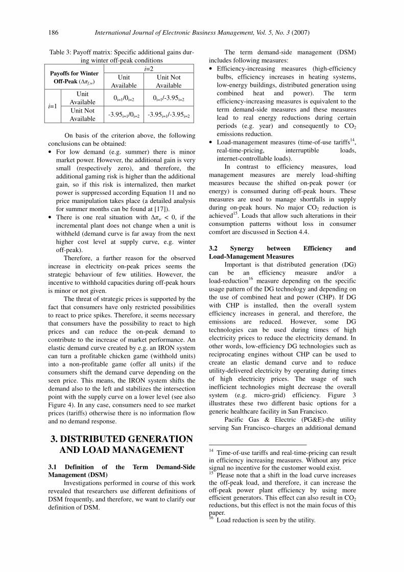
Figure 6 gives an overview of basic storage

characteristics. Having mapped the different options

of load management to conceptual storage

characteristics, each activity can be modelled with an

individual set of parameters

{P0, Tcharge, Tuncharge, Tstore, Tnostore}, where

P0 the power amplitude,

Tcharge the time to charge the conceptual storage

Tuncharge the time to discharge the conceptual stor-

age (in some cases this time is smaller

then Tcharge due to losses in the process)

Tstore the storage time

Tnostore the minimum time between two storage

operations (not depicted in Figure 6)

More complex procedures, e.g. those where

different power amplitudes are involved for the

conceptual charging and discharging can be described

by superposing multiple scaled instances of the basic

prototypes25.

25 Please note that a pre-charge storage basic concept also exists, but is not used in this work. Basic load shifting, load interruption, and load shedding can be described with a post-charge storage only.

190 International Journal of Electronic Business Management, Vol. 5, No. 3 (2007)

Figure 6: Basic Storage Characteristics

4.5 One More Degree of Freedom

The major application for load management in

our perspective is peak-load reduction due to load

shifting. Peak-load reduction will be taken as an

example for the following discussion, but the general

concept can also be applied to other demand-side

applications, such imbalance energy and other

auxiliary services.

Storage should hold energy in times of low

electricity prices and release it in times of peak

demand and prices. This is valid for real storage such

as pumped storage schemes as well as conceptual

storages as described in the previous section.

Conceptual storages are available in large numbers,

but they are distributed and have restricted individual

storage capacities. Furthermore, many distributed

storages have very short storage times, which appears

to be one reason that utilization of distributed

storages was regarded as ineffective in the past.

However, the collective (because networked) storage

capability is considerable. Each conceptual storage i

can hold the energy;

Ei = P0,i ·Tcharge,i (13)

If Ei is seen as an ”energy packet”, which can

reside in a conceptual storage for a certain time Tstore,i,

then the objective of peak-load reduction can be

re-formulated: shift as many (and as large) energy

packets as possible from off-peak to on-peak times.

This rather sophisticated description of on-peak

demand reduction leads to a new insight, which is

simple, but allows an additional degree of freedom in

resource allocation: if a single (conceptual) storage is

not able to hold an energy packet long enough, then it

can be transferred to other storages after the storage

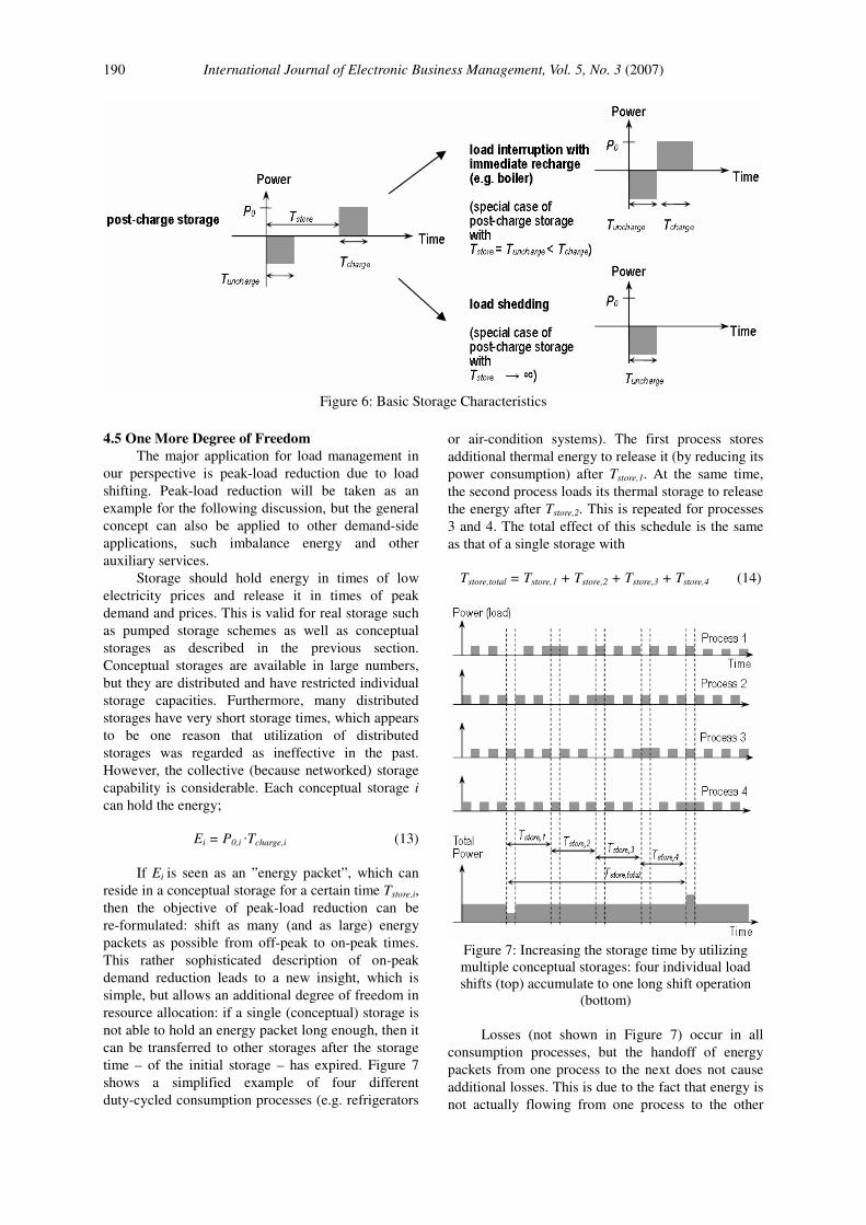
time – of the initial storage – has expired. Figure 7

shows a simplified example of four different

duty-cycled consumption processes (e.g. refrigerators

or air-condition systems). The first process stores

additional thermal energy to release it (by reducing its

power consumption) after Tstore,1. At the same time,

the second process loads its thermal storage to release

the energy after Tstore,2. This is repeated for processes

3 and 4. The total effect of this schedule is the same

as that of a single storage with

Tstore,total = Tstore,1 + Tstore,2 + Tstore,3 + Tstore,4 (14)

Figure 7: Increasing the storage time by utilizing multiple conceptual storages: four individual load shifts (top) accumulate to one long shift operation

(bottom)

Losses (not shown in Figure 7) occur in all

consumption processes, but the handoff of energy

packets from one process to the next does not cause

additional losses. This is due to the fact that energy is

not actually flowing from one process to the other


process nor is electrical energy factually stored in a

releasable way. In fact, just a subtle coordination of

DSM resources is applied in order to achieve a

modulation of the overall power consumption that is

equal to that achieved by a real storage.

With this new approach, we can achieve larger

capacities by means of parallel operation and longer

storage times by means of serial operation. Since a

large number of single resources can be utilized, any

combination of both options is possible. If all

resources have the same properties, then all

achievable combinations would be given by Equation

15,

E · Tstore = const. (15)

meaning that the total energy stored in the system E

and the duration it can be stored Tstore are two pa-

rameters that can be chosen freely as long as their

product stays constant. This constant is sys-

tem-specific.

But since each individual resource i has its own

set of {Ei, Tstore,i, Tnostore,i}, only the summation of all

individual terms is constant;

.constKTEi

i

iK

storei

i

∑∑∀∀

==⋅43421

(16)

Ki describes the abstract storage potential of one

individual conceptual storage i. This can be clarified

with the following example: The objective of shifting

the energy E from t to t+T can be achieved in two

different ways using two different basic resources

with different Ei and TStore,i. First, each resource is

able to store Ei = ½E for TStore,i = T, or secondly, each

resource is each able to store Ei = E for TStore,i = ½T.

For both cases, Ki = ½E·T is the same. 4.6 Collective Storage Management

Having described a unified description of DSM

resource behaviour, this can be used to generate

optimal schedules for the distributed storage system.

The term ”optimal schedule” is used in a more

specific way here. We assume an objective that shall

be achieved by the DSM resource collective. The

collective will not be able to meet the objective

perfectly under any circumstances. For an optimal

schedule, the distance to the objective (according to a

certain distance metric) is minimized. The objective

function can be individual energy cost reduction. In

this case, each individual storage does its best to

reduce consumption in high-price times. A storage

with arbitrary storage time examines the anticipated

price curve and searches for the lowest and highest

point. Then, it charges at the minimum and discharge

at the maximum of the price curve.

Alternatively, a resource with restricted storage

time searches for the highest slope in the prospected

price curve, since here the maximum gain can be

achieved.

More sophisticated resource scheduling is

needed for another kind of objective: load curve

following. The idea here is to control all distributed

resources as they were one large single storage26. A

large collective can have considerable capabilities

and can e.g. be used for peak-shaving. The collective

behaviour is controlled by defining a load curve that

is followed (as good as possible) by the distributed

resources. This is particularly interesting in the

context of demand charges, where a large percentage

of the energy bill is constituted by costs for the

largest monthly or yearly peak demand (see also

[17]).

In Figure 8 an example for optimal load curve

following is depicted. Twenty thermal processes, A01

to A20, with similar properties (arbitrary storage

time, equal storage energy) were assumed in this

example. Nevertheless, similar results can be

achieved with other storage types, i.e. with restricted

storage time. The comparison of specified and

achieved load curve is shown at the top. Below that,

the charge / discharge schedule for some of the

resources is depicted. Not shown in Figure 8 is the

actual power consumption of the loads used as DSM

resources, which would simply add up to a constant

offset.

This schedule is the result of an offline

optimization. A precise mathematical description of

the resource behaviour constrains the problem of

minimizing the integral difference to the target

curve 27 . In a real-world application, a more

sophisticated algorithm is needed that still uses

offline results as a guideline but is able to react on

real-time events such as resource outage due to e.g.

communication failure or unexpected discharge. The

detailed algorithm can be found at appendix A.

5. THE IRON

INFRASTRUCTURE 5.1 Communication within the Electricity System

The key to the Integral Resource Optimization

Network is the self-controlled operation of DSM

resources, and therefore, it heavily relies on a

communication infrastructure. The control strategies

26 This concept is somewhat similar to the concept of virtual power plants, where (primarily) distributed generators are controlled as a single unit. However, in our approach the focus is on storage and not on generation. 27 The mixed-integer optimization problem was described using ZIMPL [9] and solved using SCIP [1].


192

can contain energy price broadcasting or precisely

coordinated operation of distributed storages (and

supply capacities). The rapid growth of information

technology (IT) related services and equipment over

the past decades went along with a strong decline in

costs for IT equipment. Hence, communication

systems needed for coordinated DSM were already

considered to be affordable in the 1990s (see also

[14]). However, by now there is merely no

information flow in the electricity systems besides

remote control of transformer stations and data

accounting. We see the reasons for that in the highly

diversified interests of different players such as

distribution grid operators, energy providers and

consumers, and in the lack of standardization of

remote metering and control systems. In the frame of

the IRON project, a common information

infrastructure is specified that is able to meet the

needs of distributed DSM algorithms and can handle

the vast growing number of connected sites. The

challenge is to identify a suitable and flexible

network topology together with a protocol that is

open for future enhancements. Furthermore, the

connection interface between the IRON and the

electrical equipment has to be specified (see also

Figure 9).

Figure 8: Example of twenty similar DSM resources optimally scheduled so that that the sum of charging and

discharging powers follow a given load curve as close as possible. Only the differential power consumption is

shown

Control Centre

Load

Interface

Load Load Load

Access Servers

Optional On-site Sub-Network

IRO

N

Figure 9: Structure of the prospected IRON commu-

nication system.

Given the possibly large number of single

communication nodes that are going to be connected

by the IRON communication infrastructure, only a

hierarchical network structure appears useful (see

Figure 9).

Due to cost restrictions, the top-level

(long-distance) infrastructure can be implemented

only by using existing communication networks,

predominantly the Internet and Telecom networks.

Different types of end-user equipment and on-site

sub-networks are connected to the access servers of

this top-level network. The size and structure of these

sub-networks depend on the kind of entity: for an

industrial plant an already present automation


infrastructure can be used, while for an office

building an already present building automation

network can be used. In case that no other automation

infrastructure is present, the interface between load

and IRON is realized by using an “IRON-Box”.

5.2 The IRON-Box

The IRON-Box realises the interface between

the DSM resource (e.g. load) and the IRON. Since

freely configurable equipment for load management

is not available as COTS (commercially

off-the-shelve) products, the IRON team has been

developed a prototype, which is depicted in Figure

10. The prototype serves as hardware equipment for

experiments as well as a basis for estimating the costs

for a commercial production. The device features

optional WLAN (Wireless Local Area Networks) or

mobile network (General Packet Radio Switched

Network, GPRS) data connection on the

infrastructure side. A small on-board processor

manages the communication flow and local control

loops. On the load side, two channels with one relay

output, three digital inputs and one power sensor each

are available. Using the power sensor, the IRON-Box

can measure the power consumption patterns of the

connected load and generate statistics about the load

utilization, which can be used to optimize load

schedules. The relays allow switching on / off the

connected loads according to the optimization

algorithm used.

Communication Interface (e.g. Mobile Network)

Processor Memory

Digital Inputs

Power Sensor

Relay

Digital Inputs

Power Sensor

Relay

Figure 10: Main components of the IRON-Box

Additionally, measurement equipment (e.g.

energy meters or temperature sensors) can be

connected to the digital inputs. The IRON-Box can

work together with (or even replace simple)

controllers for air conditioning systems or

refrigerators.

The experimental unit has a size of 75 x 70 x

110 mm. It consists of 120 components that account

for material costs of 230 Euro (single unit in very low

volume). Still, large potentials for optimization in

terms of size, complexity and costs exist. Considering

prices for comparable mass-market products, we

anticipate that the device could be manufactured for

costs well below 100 Euro.

6. CONCLUSIONS

Load-management measures, used to manage

lack in supply during on-peak hours, allow alteration

in the consumption pattern without loss in consumer

comfort and can create a short-term elastic demand

curve. Such measures can be coordinated by an

Integral Resource Optimisation Network–”IRON”,

which indicates a robust and distributed automation

network for the optimization of distributed usage and

supply.

Because of the current situation on the

electricity markets and, particularly, due to the lack of

an elastic demand curve in the short term, the threat

of strategic prices is increasing. It seems necessary

that consumers have the possibility to respond to high

prices and can reduce the on-peak demand in order to

contribute to the increase of market performance. An

elastic demand curve, which can be achieved by

using the discussed IRON System, can turn a

profitable chicken game (withhold units) into a

non-profitable game (offer all units) if the consumers

shift the demand depending on the charged price (e.g.

real-time pricing). In any case, consumers need to see

tariffs based on the market prices otherwise there is

no information flow and no demand response.

Additionally, the combination of CHP-enabled

technologies and load-management measures to

reduce on-peak demand seems the most favourable

option for a distributed automation network as the

IRON. With the IRON system, we want to establish a

holistic optimization algorithm for distributed supply

and demand. This new algorithm can be applied to a

single site or a combination of distributed sites.

The IRON System offers a new solution to

integrate participants which have been considered

unreachable in conventional structures of

contemporary electricity markets. It has been shown

that the potential of distributed resources can be

exploited by applying the concepts of storage

modelling on load shift measures as well as serial and

parallel operation of such real or conceptual storages.

Despite strong restrictions in individual resources, the

collective system is very flexible.

The fact that all participants are equally capable

of exerting influence on the consumption and use of

the electrical “resources” means a great economic and

socio-economic benefit. This reduces the impact of

disadvantages and problems caused by the

insufficiently liberalized contemporary electricity

markets without a short term elastic demand curves.


194

Unlike traditional means of demand side control the

described IRON System exploits unused optimization

potentials without negatively influencing the

customers’ processes or comfort. The system acts in

the background, in a distributed, discrete and flexible

manner. The implemented hardware prototype

(IRON-Box) that interfaces an individual load with

the IRON System allows cost estimates for the IRON

infrastructure. Given the current situation of rapidly

decreasing costs for information and communication

technology on one hand and steadily rising energy

prices on the other hand it is just a matter of time

when the benefit of coordinated short-term DSM

measures is broadly realized.

REFERENCES

1. Achterberg, T., 2004, “SCIP-A framework to

integrate constraint and mixed integer programming,” ZIB report 04-19, Berlin.

2. Bobinaitė, V., Juozapavičienė, A. and Snieška, V., 2006, “Correlation of electricity prices in European wholesale power markets,” Engineering Economics, Vol. 49, No. 4, pp. 7-14.

3. California Energy Commission, 2005, “Enhanced automation case study 7, lighting and equipment controls/grocery store,” California Energy Commission.

4. Firestone, R. M., Stadler, M. and Marnay, C., 2006, “Integrated energy system dispatch optimization,” The 4th International IEEE

Conference on Industrial Informatics,

INDIN’06, pp. 16-18. 5. Halseth, A., 1999, “Market power in the Nordic

electricity market,” Utilities Policy, Vol. 7, No. 4, pp. 259-268.

6. Hebner, R. Beno, J. and Walls, A., 2002, “Flywheel batteries come around again,” IEEE

spectrum, Vo. 39, No. 4, pp. 46-51. 7. Section: Environment and Energy, Folder:

Energy Statistics–Prices: http://epp.eurostat.ec.europa.eu.

8. Energy Information Administrator, http://www.eia.doe.gov.

9. Koch, T., 2004, “Rapid mathematical programming,” Technische University, Ph. D

Dissertation. 10. Müsgens, F., 2004, “Market power in the

German wholesale electricity market,” EWI

Working Paper, Graduate School of Risk Management and Institute of Energy Economics at the University of Cologne.

11. Piette, M. A., Watson, D. S., Motegi, N. and Bourassa, N., 2005, “Findings from the 2004 fully automated demand response tests in large facilities,” LBNL Report.

12. Schreiber, M., Whitehead, A. H., Harrer, M. and Moser, R., 2005, “The vanadium redox

battery-An energy reservoir for stand-alone ITS applications along motor and expressways,” Proceedings of Intelligent Transportation

Systems, pp. 391-395. 13. Siddiqui, A. S., Firestone, R. M., Ghosh, S.

Stadler, M., Marnay, C. and Edwards, J. L., 2003, “Distributed energy resources customer adoption modeling with combined heat and power applications,” Lawrence Berkeley

National Laboratory Report, Lawrence Berkeley National Laboratory.

14. Smith, H. L., 1994, “DA/DSM directions: An overview of distribution automation and demand-side management with implications of future trends,” Computer Applications in

Power, Vol. 7, No. 4, pp. 23-25. 15. Stadler, M., 2003, “The relevance of

demand-side-management and elastic demand curves to increase market performance in liberalized markets: The case of Austria,” Dissertation Vienna University of Technology.

16. Stadler, M., Palensky, P., Lorenz, B., Weihs, M. and Roesener, C., 2005, “Integral resource optimization networks and their techno-economic constraints,” International

Journal of Distributed Energy Resources, Vol. 1, No. 4, pp. 299-320.

17. Stadler, M., Firestone, R. M., Curtil, D. and Marnay, C., 2006, “On-site generation simulation with energy plus for commercial buildings,” ACEEE Summer Study on Energy

Efficiency in Buildings. 18. Stadler, M. and Auer, H., 2002, “A simple

game of supply-empirical part, the Nordic power market,” Working Paper, Vienna

University of Technology.

ABOUT THE AUTHORS

Michael Stadler joined Berkeley Lab as a student in

2002, returned as Post-Doctoral Fellow in 2005, and

is currently a Visiting Scholar. In December 2006 he

founded the Center for Energy and innovative

Technologies, which he has been heading since then.

He also supported the University of California,

Berkeley’s Pacific Region CHP Application Center,

where he conducted site analyses of varied

commercial, agricultural, and industrial CHP projects.

Previously, he worked with the Energy Economics

Group at the Vienna University of Technology, from

which he holds a Masters degree in electrical

engineering and a Ph.D. summa cum laude in energy

economics. His fields of research are distributed

energy, electricity markets, and demand response.

Friederich Kupzog achieved the Diploma Engineer

degree of electrical engineering and information

technology at RWTH Aachen University of

Technology in February 2006. The focus of his


studies was on communication and VLSI circuit

design. He joined the Institute of Computer

Technology at Vienna University of Technology,

Austria, in March 2006 as a Project Assistant. His

main research interest lies in applications of modern

information and communication technologies in

energy transmission and distribution. Currently, he is

working on his PhD thesis in this field.

Peter Palensky is senior researcher at Vienna

University of Technology, teaching Microcomputer

Architecture and distributed systems. He is working

on wide area control networks, dependable networked

embedded systems, building automation and energy

automation. Besides leading several research projects,

he is actively engaged in ISO, IEEE and CEN.

(Received April 2007, revised June 2007, accepted

August 2007)

APPENDIX: MODEL USED FOR

OPTIMIZATIONS

As outlined in Section 4.4, DSM resources can

be modelled by the linear superposition of basic

storage characteristics. Consequently, it is possible to

translate the scheduling problem of DSM resources

into a linear optimization problem. In order to avoid

the following discussion becoming unnecessarily

complex, the optimization problem shall only be

discussed for resources with arbitrary storage time

Tstore.

DSM resources can either be charged or

discharged, resulting in a positive or negative

contribution to the load profile. Two series cn,i and dn,i

can be defined, so that

cn,i = 1 for n is the centre time slot of a

charging process for resource i, or 0 other-wise,

(17)

and

dn,i = 1 for n is the centre time slot of a discharging process for resource i, or 0

otherwise. (18)

It is useful to split charging and discharging

into two series, so that the total number of charging

processes per resource can easily be restricted by

expressions like

mcn

in <∑∀

,

(19)

without having to operate with absolute values.

Nevertheless, a single series an,i = cn,I – dn,i (20)

can also be defined, that includes both charging and

discharging information. In an,i, cn,i, and dn,i, only one

element is non-zero for each charging or discharging

process.

Each resource has its individual charge and

discharge profile. These profiles can also be

described as series. The convolution of the impulse

series cn,i and dn,i with these time-discrete load

profiles fn,i and gn,i result in the actual (time-discrete)

power consumption pn,i of the resource n as described

in (21). This equation is actually a linear constraint

equation to the optimization problem since it

constraints pn,i in regard to the previously defined

variables.

iln

l

ilikn

k

ik

ininininin

gdfc

gdfcp

,,,,

,,,,,

−

∞+

−∞=

−

∞+

−∞=

∑∑ −

=∗−∗=

(21)

When calculating the convolution, the sum

index has only to cover those terms that are non-zero.

In the following discussion it will always assumed

that all processes are fully scheduled in the time

interval [0, Tend] with no process overlapping the

borders of this interval. In this case, the convolution

can be calculated as shown in (22) and thus has a

finite number of terms.

kn

T

k

knn babaend

−

=

∑=∗

0

(22)

Furthermore, the energy level sn,i of resource n

can be defined as

∑=

=

n

t

itin ps0

,, . (23)

To sum up the previous variable definitions, the

impulse series cn,i and dn,i are the actual unknown

variables defining the schedule of charging and

discharging processes that shall be determined by the

optimization. Power pn,i and energy level sn,i are

derived from them and are needed in the objective

function and further constraints respectively.

The objective function subtracts the achieved

overall load profile ptot,n from the required profile

preq,n:

min,0

,

0

,

0

,,

→−

=−

∑ ∑

∑

= =

=

end

end

T

n

nreq

N

i

in

T

n

nreqntot

pp

pp

(24)

(where N is the total number of resources). The

absolute value of the difference is used in order to

keep the problem piecewise linear (it is possible to

translate (24) into a set of linear equations with


196

restricted index ranges [9]). From an application

perspective, the square of the difference would be

preferable, but in that case the problem cannot be

solved by solver for linear problems.

Further constraints of the problem are restricted

storage capacity:

iini SsS max,,min, ≤≤ (25) restricted charge and discharge frequency: the impulses in cn,i and dn,i must not come too close to each other (refer to Tnostore in Section 4.4). The resource may need some time to settle on a certain energy level until the next set-point change can occur. A possibility to express this in a linear equation is to make use of a distance series

δn,i = 1 for n = 0 … Tcharge+Tnostore, 0 otherwise,

(26)

and to restrict the amplitude of the convolution of

distance series and impulse series. Depending on

the restrictions of actual resources it may be nec-

essary to define separate δ series for charging and

discharging or even to formulate more complex

constraints.

1)( ,,,, ≤∗+= inininin dct δ (27)

Documents

DISTRIBUTED ENERGY RESOURCE ALLOCATION … AN ECONOMIC AND TECHNOLOGICAL ... Distributed Energy Resource Allocation and Dispatch 183 ... reference for the marginal power plant