1

Distributed Cross-Layer Algorithms for the OptimalControl of Multi-hop Wireless Networks

Atilla Eryilmaz, Asuman Ozdaglar, Devavrat Shah, and EytanModiano

Abstract— In this paper, we provide and study a general frame-work that facilitates the development of distributed mechanismsto achieve full utilization of multi-hop wireless networks. In par-ticular, we describe a generic randomized routing, scheduling andflow control scheme that allows for a set of imperfections in theoperation of the randomized scheduler to account for potentialerrors in its operation. These imperfections enable the design ofa large class of low-complexity and distributed implementationsfor different interference models. We study the effect of suchimperfections on the stability and fairness characteristics of thesystem, and explicitly characterize the degree of fairnessachievedas a function of the level of imperfections. Our results reveal therelative importance of different types of errors on the overallsystem performance, and provide valuable insight to the designof distributed controllers with favorable fairness characteristics.

In the second part of the paper, we focus on a specificinterference model, namely the secondary interference model,and develop distributed algorithms with polynomial communi-cation and computation complexity in the network size. Thisisan important result given that earlier centralized throughput-optimal algorithms developed for such a model relies on thesolution to an NP-hard problem at every decision. This resultsin a polynomial complexity cross-layer algorithm that achievesthroughput optimality and fair allocation of network resou rcesamongst the users. We further show that our algorithmic ap-proach enables us to efficiently approximate the capacity regionof a multi-hop wireless network.

Index Terms— Multi-hop Wireless Networks, Network Op-timization, Randomized Algorithms, Congestion Control, FairAllocation, Throughout-optimal Scheduling, Dynamic Routing.

I. I NTRODUCTION

There has been considerable recent interest in develop-ing network protocols to achieve the multiple objectivesof throughput maximization and fair allocation of resourcesamong competing users. Much of the work in wireless commu-nication networks has focused on centralized control and hasdevelopedthroughput-optimalpolicies (e.g. [43], [32], [16]).However, these policies do not directly lend themselves to dis-tributed implementation, which is essential in practice. In thispaper, we provide a class of randomized routing, schedulingand flow control algorithms that achieve throughput-optimaland fair resource allocations that is amenable to distributedimplementation with polynomial communication and compu-tation complexity.

Atilla Eryilmaz is with the Ohio State University{eryilmaz@ece.osu.edu}.Asuman Ozdaglar, Devavrat Shah, and Eytan Modiano are with the Mas-sachusetts Institute of Technology{{asuman, devavrat, modiano}@mit.edu}.This work was supported by: DTRA grant HDTRA1-08-1-0016; the Control-Based Mobile Ad-Hoc Networking (CBMANET) Program under DARPAsubcontract no. 060786; and ARO Muri grant number W911NF-08-1-0238.

In their seminal work, Tassiulas and Ephremides developeda joint routing-scheduling algorithm that stabilizes the networkwhenever the arrival rate of the exogenous flows are withinthe stability (capacity) region. In [42], Tassiulas showedthatrandomized algorithms can be used to achieve maximumthroughput in input queued switches with linear computa-tional complexity. To improve the exponentially high delayperformance of [42], [19] introduced randomized algorithmsfor switches. Other research, for example, [24], [36], [39],[32], [1], [16], [37], [38], have contributed to the analysis ofcentralizedthroughput optimal policies in wireless networks.

In this work, we provide a scheduling-routing algorithmcombined with a congestion controller for a general systemmodel whereby multi-hop flows are considered. Following theapproach of [29], we allow various types of errors to occurduring the scheduling operation, which facilitates the designof distributed implementations. One of the main contributionsof the paper is the explicit characterization of the effect ofdifferent types of errors on the overall performance. Addition-ally, this paper contributes to the study of resource allocationin multi-hop wireless networks in several fundamental ways.

First, we propose a generic cross-layer mechanism withthree components: a randomized scheduling component and arouting component (implemented by the network nodes) aimedat allocating resources to the flows efficiently; and a dualcongestion control component (implemented at the sources)aimed at regulating the flow rates to achieve fairness. To facili-tate distributed implementation, several types of imperfectionsare allowed in the scheduler, as in [29]. In this work, wefurther add a routing component to the framework to optimallysteer multi-hop traffic, and a congestion control componentthat regulates the flow rates to achieve fair division of theresources among flows, wherefairness is defined using theutility-maximization framework of Kelly et al. [22], [23] andfurther improved in subsequent works [27], [46], [40].

Second, we study the proximity of the achieved rate alloca-tion with generic cross-layer scheme to the fair allocation, andexplicitly characterize the performance loss as a functionofthe imperfections of the underlying scheduler. Moreover, byrevealing the relative importance of different types of errorson the performance, our analysis also yields principles forefficient design of distributed network controllers.

Third, for the secondary interference model1, we show thatour cross-layer mechanism can be implemented via distributed

1In the secondary interference model, two links interfere ifthey share anode or if there is a link that connects any of the end nodes of the two links.This interference model prevents real world issues such as the hidden terminalproblem (see [33]).

2

algorithm. This approach involves the operation of two sequen-tial algorithms. A novel feature of these algorithms is theiroperation on an appropriately constructed conflict graph. Theuse of the conflict graph leads to a partitioning of the network,whereby the decisions can be made independently in differentpartitions. Moreover, the operations on the conflict graph canbe mapped into network level operations using the specialstructure of the problem. These distributed algorithms notonlyachieve throughput-optimal and fair allocations, but alsohavepolynomial communication and computation complexity.

Finally, our policy suggests an algorithmic method of es-timating the stability region of multi-hop wireless networks,which is otherwise a very difficult task to characterize.

This work differs from our earlier relevant works [12], [13],[14] in that: [12] studies the performance cross-layer algorithmwith a pick-and-compare scheduler, but without any errorsand does not propose any specific implementable algorithm;[13] proposes a low-complexity algorithm, but still does notallow for any errors; [14] allows for errors but only allowssingle-hop traffic and thus has no routing component. Otherrelated works include [11], [28], [26], [44], which developdistributed algorithms that guarantee50% utilization of thestability region for a primary interference model2. Whiledistributed implementation of these algorithms is possible,this comes at the cost of sacrificing a significant portion ofthe capacity of the network (see, for example, [6], [5]). Asmore general interference models are considered, even moreof the capacity of the network needs to be sacrificed fordistributed implementation (e.g., [45], [7]). For example, in thecase of a secondary interference model with the grid topology,distributed implementation can only guarantee12.5% of thecapacity of the network. [29] also used [42] to developdistributed schedulers by utilizing Gossip mechanisms.

More recently, the throughput performance of greedy max-imal matching schedulers are investigated for general interfer-ence models and geometric graphs ([20]), which proves that1/6 of the stability region is guaranteed to be achievable bysuch schedulers. In other recent works ([21], [4]), distributedschedulers are proposed with attractive delay characteristics.

The rest of the paper is organized as follows. In Section II,we describe the system model and our goal. In Section III, wedescribe a generic randomized scheme for scheduling-routing-congestion control, and prove its throughput-optimality andfairness properties. In Section V, we use the randomizedscheme to design and analyze distributed algorithms for thesecondary interference model. Finally, in Section VI we pro-vide simulation results.

Throughout the paper, we denote the dot product of twovectors, sayX andY, as 〈 X,Y〉.

II. SYSTEM MODEL AND GOAL

Consider a wireless network that is represented by anundirected graph,G = (N ,L), which has a node setN (withcardinalityN ), a link setL (with cardinalityL). We assume atime slotted system with synchronized nodes, where each slotis long enough to accommodate a single packet transmission

2In the primary interference model, each feasible allocation consists of linksthat do not share a node, i.e. each feasible allocation is amatching.

over each link inL unless there is interference. We refer to theflow that enters the network at noden and leaves it at noded as

Flow-(n, d). We let X[t] =(

X(d)n [t]

)d∈N

n∈Ndenote the vector

of arrivals to the network in slott with X(d)n [t] corresponding

to the arrivals for Flow-(n, d). We use the notationx(d)n [t]

to denote themean flow rate of Flow-(n, d) in slot t, i.e.,x

(d)n [t] = E[X

(d)n [t]]. Then, themean flow rate of Flow-(n, d)

is defined asx(d)n = limT→∞

1T

∑T−1t=0 x

(d)n [t] whenever it

exists.We consider a general interference model specified by a

set of link-pairs thatinterfere with each other, i.e., whentheir concurrent transmissions collide. We assume that if twointerfering links are activated in a slot, both transmissionsfail. Note that this includes a large class of graph-theoreticinterference models considered in the scheduling literature(e.g. the primary interference model [35], [26], [44], [6],orthe secondary interference model [2], [45], [7]).

We useS[t] =(

S(n,m)[t])

(n,m)∈Lto denote a linkalloca-

tion vector(or schedule) at timet, andS to denote theset offeasible allocationswhere a feasible allocation is a set of linksin which no two links interfere with each other. We introducethe notationS(d)

(n,m) to distinguish packets destined for different

nodes: at any given slott, S(d)(n,m)[t] ∈ {0, 1} is 1 if link

(n,m) serves a packet destined for noded in that slot, and0otherwise. This implies that

∑

d∈N S(d)(n,m)[t] = S(n,m)[t], for

all (n,m) ∈ N .At each node, a buffer (queue) is maintained for each

destination. We letQ(d)n [t] denote the length of the queue at

noden destined for noded at the beginning of slott. Evolutionof Q(d)

n [t] whenn 6= d satisfies

Q(d)n [t+ 1] ≤

(

Q(d)n [t] − S

(d)out(n)[t]

)+

+X(d)n [t] + S

(d)in(n)[t],

(1)

where(y)+ = max(0, y). Also,

S(d)in(n)[t] ,

∑

{k:(k,n)∈L}

S(d)(k,n)[t]

is a shorthand for the maximum number of packets that canbe internally routed to noden that are destined for noded. Similarly, S(d)

out(n)[t] ,∑

{m:(n,m)∈L} S(d)(n,m)[t] are the

maximum number of packets that can leave noden and aredestined for noded. When,n = d, we setQ(d)

d [t] = 0, for allt, because in that case the packets have already reached theirdestination.

Next, we introduce the concepts of network stability andcapacity region.

Definition 1 (Stability): A given queue, sayQ(d)n , is stable

if lim supT→∞

1

T

T−1∑

t=0

E[Q(d)n [t]] <∞. The network isstableif all

queues are stable; andunstableotherwise.Definition 2 (Capacity [Stability] Region C): The capac-

ity (stability) regionC is the set of(x(d)n )n,d∈N ≥ 0 for which

there exists an algorithm that can stabilize the network3.

3Note that, under this definition, the capacity region is monotone, i.e., ifx ∈ C, theny ≤ x (component-wise) must also be inC.

3

Given the general model described above, our goal is to de-sign distributed algorithms that achieve throughput-optimalityand fair allocation of the network resources amongst the flows.Following the extensive literature on the topic (e.g. [43],[39],[32], [15]) we call a policythroughput-optimalif it can supportany mean flow rate in the capacity region without violating thenetwork stability.

To define fairness we use the “utility maximization” frame-work of economics: with each flow, say Flow-(n, d), weassociate a utility functionUn,d(·), of the mean flow rateswherebyUn,d(x(d)

n ) is a measure of the utility gained by Flow-(n, d) for the mean flow ratex(d)

n . We assume, based on thelaw of diminishing returns, that the functionUn,d(·) is concaveand non-decreasing for all flows. Then, a mean flow rate vector⋆x is referred to as afair allocation if it is an optimal solutionof the convex optimization problem:

⋆x ∈ arg max

x∈C

∑

n,d∈N

Un,d(x(d)n ). (2)

Hence, a fair allocation is a mean flow rate vector thatmaximizes the aggregate utility over all flows in the network.It is known that by definingUn,d(·) appropriately, differenttypes of fairness, such as proportional or max-min fairness,can be achieved ([22], [23], [27], [40], [15], [31], [25]).

III. G ENERIC CROSS-LAYER SCHEME

In this section, we provide the description of a genericcongestion control-routing-scheduling scheme that achievesthe throughput-optimality and fairness goals of Section II. Thescheme combines ideas from recently studied congestion con-trollers designed for wireless networks (e.g. [15], [31], [26],[41], [8]), and the randomized scheduling strategy introducedby Tassiulas in his seminal work [42]. Our algorithm not onlyextends the use of randomized scheme of [42] to multi-hopnetworks with general interference models, but also utilizes theparallel use of a dual congestion controller to achieve fairness.

The generic scheme is composed of three components: thescheduling and routing components that are implemented bythe network, and the congestion control component that isimplemented by the users (or the sources of the flows). Thescheduling component builds on two algorithms: one, calledPICK, which randomly picks a feasible allocation satisfying aspecific condition [see Eq. (5) below]; and the other, calledUPDATE, which contains a network-wide comparison opera-tion [see Eq. (6) below]. In the operation of PICK and UPDATE

algorithms, we allow for various types of imperfections andrelaxations to accommodate errors and to facilitate distributedimplementations. We will comment on the nature of theseimperfections and relaxations after the description of thecross-layer scheme. The routing component determines whichpackets to be served over which links so as to optimize theirroutes. Finally, the congestion controller component adjuststhe rate of injected traffic into the network to fully utilizetheresources, i.e., to solve (2).

The scheme operates instages, each stage containing afinite number of time slots where the number of slots is adesign choice. The scheduling-routing and congestion control

decision is updated at the beginning of each stage, and is keptunmodified throughout the stage.

Definition 3 (Generic Cross-layer Scheme):The cross-layer algorithm is composed of three components: arandomized scheduler with imperfections characterizedby the parameters(δ, γ, ψ); a routing component thatsteers packets towards optimal paths; and a congestioncontroller component that regulates the amount ofinjected traffic into the network to maximize the networkutilization. Next, we describe each of these components.

SCHEDULING(δ, γ, ψ) COMPONENT: The scheduling com-ponent determines the service rates of all the links inthe network, namelyS[t], by performing the followingoperations• At staget, for each link(n,m) ∈ L, we define itsweightas

W(n,m)[t] = W(m,n)[t] , maxd

∣

∣

∣Q(d)n [t] −Q(d)

m [t]∣

∣

∣,(3)

which is also referred to as themaximum differential backlog([32], [16]) of link (n,m).

• Let theoptimum feasible allocation⋆

SW [t] for W be⋆

SW [t] ∈ arg maxS∈S

∑

l∈L

wl[t]Sl ≡ arg maxS∈S

〈 W[t],S〉

= arg maxS∈S

〈 Q[t],Sout − Sin〉, (4)

whereSout andSin are defined subsequent to (1).• PICK : Scheduler randomly picksany feasible allocationR[t] ∈ S, that satisfies, for some fixedδ > 0,

P(R[t] =⋆

SW [t]) ≥ δ, for all W[t] and t. (5)

• UPDATE: The schedule for timet, S[t] is updated suchthat it satisfiesP (〈Q[t],Sout[t] − Sin[t]〉 ≥

max {〈Q[t],Sout[t− 1] − Sin[t]〉,(1 − γ)〈Q[t],Rout[t] − Rin[t]〉}) ≥ 1 − ψ,

(6)

for someγ, ψ ∈ [0, 1).

ROUTING COMPONENT: Once the link rate vectorS[t] isdetermined by the scheduler, the router determines whichpackets to transmit over them.• Let d⋆nm = d⋆mn , arg maxd

∣

∣

∣Q

(d)n [t] −Q

(d)m [t]

∣

∣

∣. Then,

– if Q(d⋆

nm)

n [t] ≥ Q(d⋆

nm)

m [t] : ServeS(n,m)[t] packets from

Q(d⋆

nm)

n to Q(d⋆

nm)

m , and– if Q(d⋆

nm)

n [t] < Q(d⋆

nm)

m [t] : ServeS(n,m)[t] packets from

Q(d⋆

nm)

m to Q(d⋆

nm)

n .

Before describing the congestion controller component, weremark that the parameters(δ, γ, ψ) in the above schedulercapture different type of imperfections and relaxations:δrelaxes the constraint of picking the optimum feasible al-location in each iteration, hence significantly reduces thecomplexity of this operation;γ captures the potential errors inthe computation of the total weight of the randomly selectedschedule; andψ captures the potential errors in the comparisonof the weights of the previous and the random scheduler.

4

The imperfections included in the scheduling component arelikely to occur when randomized or distributed methods areemployed to perform these operations.

DUAL CONGESTIONCONTROL COMPONENT:• Let Q denote the queue-length vector at the beginning ofstaget. Then, each node, sayn, generatesX(d)

n [t] packetsto be transmitted to noded, for eachd, such that

X(d)n [t] =

{

U ′−1n,d

(

Q(d)n [t]

K

)}M

0

, (7)

whereM andK are positive scalars, and{z}ba is used todenotemin(max(z, a), b).Notice that (7) is equivalent to solving

X(d)n [t] = argmax

y∈[0,M ]

(

KUn,d(y) − y Q(d)n [t]

)

, (8)

and also, note that if there exists no flow fromn to d, wecan defineUn,d(·) ≡ 0 to getX(d)

n ≡ 0.

Our goal in this work is to understand the effect of theimperfections captured by(δ, γ, ψ) parameters on the optimal-ity (or fairness) characteristics of the cross-layer mechanism.Our framework covers various schedulers that are introducedin the literature (e.g. [42], [29], [34]). In particular, [34]yields a scheduler for the first-order interference model withγ = 1/m, andψ = 0, wherem is a design parameter. Also,[29] contain algorithms withγ = ψ = 0, as well as gossip-based algorithms with arbitrarily smallγ, ψ parameters. Noneof these works, however, contain a study of the cross-layerscheme with congestion control. Hence, our analysis of thegeneric cross-layer scheme will be directly applicable to allthese cases. In Section V, we will introduce a new algorithmthat is applicable to higher order interference models, anduseour results to show that it achieves optimality using operationsthat grow polynomially with the number of nodes.

IV. A NALYSIS

In this section, we study the throughput-optimality andfairness properties of the proposed generic cross-layer scheme.Our analysis relies on the notions ofε-relaxed stability regionandε-fair allocation, which we define next.

Definition 4 (ε-relaxed stability region,C(ε)):

C(ε) , {x ≥ 0 : (x(d)n + ε)n,d∈N ∈ C}.

Definition 5 (ε-fair allocation,⋆x (ε)):

⋆x (ε) = arg max

x∈C(ε)

∑

n,d

Un,d(x(d)n )

Note that asε ↓ 0, we have⋆x (ε) →⋆

x . Let us define a newstate,Y := (Q,S), which forms a Markov Chain under ourgeneric cross-layer scheme.

In the following theorem, we focus on the scheduling-routing component of the algorithm by assuming that themean flow rates lie inside theε-relaxed stability region. Here,we assume that the arrivals are inelastic, i.e., their statisticsare not modified throughout the operation of the scheduling-routing component. Later, we will add the congestion controlcomponent into the framework.

Theorem 1:Assume thatX(d)n [t] is independent and iden-

tically distributed (i.i.d.) 4 for all t and flows with

E

[

(

X(d)n

)2

[1]

]

≤ A < ∞. Assume thatε > 0 is chosen

such that εdmax

> γ2 +√

ψδ(1−ψ) , wheredmax is the maximum

degree of the network, andδ, ψ, andγ are the parameters ofthe generic cross-layer scheme.

Let the Lyapunov functionV (Y) be defined asV (Y) =∑

n,d

(

Q(d)n

)2

= ‖Q‖22. Then, for any mean arrival vectorλ :=

(

E[X(d)n [1]]

)

n,d∈N∈ C(ε), the scheduling-routing(δ, γ, ψ)

policy guarantees, for some finiteT,

∆V(T )t (Y) , E [V (Y[t+ T ]) − V (Y[t]) |Y[t] = Y]

≤ −cT(

ε

dmax− γ

2−√

ψ

δ(1 − ψ)

)

∑

n,d

Q(d)n +B1,

whereB1 is a bounded positive number, andc is a positiveconstant.

Proof: The proof is moved to the Appendix.An immediate consequence of Theorem 1 is provided next.

Corollary 1: The generic cross-layer algorithm stabilizesany traffic with a mean flow rate vector lying insideC(

dmax

(

γ2 +

√

ψ/(δ(1 − ψ))))

.

Proof: Pick ε to be larger but arbitrarily close todmax(γ/2 +

√

ψ/(δ(1 − ψ))). Then, from Theorem 1, wehave

∆V(T )t (Y) ≤ −ε′

∑

n,d

Q(d)n +B1,

for some ε′ > 0. This shows that the Foster-Lyapunovcriterion is satisfied (see e.g. [3]), and therefore we must havelim supT→∞

1T

∑T−1t=0

∑

n,d E[Q(d)n [t]] <∞.

The scheduling-routing component of the above algorithmis based on [42] whereby the existing feasible allocation iscompared to a randomly picked feasible allocation, and theone with the larger total weight is implemented in the nextstage. The same strategy is also used in a recent work [29]which develops another deterministic distributed algorithm forthe primary interference model, and randomized algorithmsbased on gossiping techniques that are applicable to moregeneral interference models. In other works (e.g. [26], [7], [6],[45], [34], [20]), low complexity implementations have beenproposed at the expense of different levels of efficiency lossfor the primary interference model. But, many of these resultsare not applicable in the higher interference models scenarios.

The next theorem studies the impact of the parameters(δ, γ, ψ) in the proposed cross-layer mechanism on its stabilityand fairness characteristics. Earlier works in this context (e.g.[31], [15], [26], [41]) are applicable only to the case of acentralized scheduler. Below, we extend these results in thepresence of a randomized scheduling-routing component withimperfections.

4The assumption of i.i.d. arrivals is not critical to the analysis. The sameresults continue to hold for processes with mild ergodicityproperties ([17]).

5

Theorem 2:For any generic cross-layer(δ, γ, ψ) scheme,there exists finite constants,C1, C2, such that: for anyε > 0

for which εdmax

> γ2 +

√

ψδ(1−ψ) , we have

∑

(n,d)∈N 2

q(d)n ≤ C1K, (9)

∑

(n,d)∈N 2

Un,d(x(d)n ) ≥

∑

(n,d)∈N 2

Un,d(

⋆x

(d)

n (ε)

)

− C2

K, (10)

whereq(d)n , lim supT→∞

1

T

T−1∑

t=0

E[Q(d)n [t]],

and x(d)n , lim

T→∞

1

T

T−1∑

t=0

E[X(d)n [t]].

Proof: The proof utilizes the Lyapunov-based analysisand the technique introduced in [31] together with Theorem 1.Recall that Y = (Q,S), and that the definition of theLyapunov function introduced in Theorem 1 is:V (Y) =∑

n,d

(

Q(d)n

)2

. Then, by using the same arguments as in thederivation of (16) and (17), it can be shown that∆V

(T )t (Y)

, E [V (Y[t+ T ])− V (Y[t]) |Y[t] = Y]

≤T−1∑

τ=0

E [V (Y[t+ τ + 1]) − V (Y[t+ τ ] | Y[t] = Y]

≤ 2

T−1∑

τ=0

E [〈Q[t+ τ ],Sin[t+ τ ] + X[t+ τ ]

−Sout[t+ τ ]〉 |Y[t] = Y] + T (b1 + b2),

for some finite constantsb1, b2 that were introducedin the proof of Theorem 1. Next, we add and sub-

tract 2KT−1∑

τ=0

E

∑

n,d∈N

Un,d(X(d)n [t+ τ ]) | Y[t] = Y

, and

re-arrange the terms to get∆V

(T )t (Y)

≤ 2K

T−1∑

τ=0

E

∑

n,d∈N

Un,d(X(d)n [t+ τ ]) |Y[t]

−2

T−1∑

τ=0

E[E[K∑

n,d∈N

Un,d(X(d)n [t+ τ ]) −

〈 Q[t+ τ ],X[t+ τ ]〉 |Y[t+ τ ]] |Y[t]]

−2

T−1∑

τ=0

E [〈Q[t+ τ ],Sout[t+ τ ] − Sin[t+ τ ] |Y[t]]

+T (b1 + b2)

Lemma 1:

E[K∑

n,d∈N

Un,d(X(d)n [t+ τ ])

−〈Q[t+ τ ],X[t+ τ ]〉 | Y[t+ τ ]]

≥ K∑

n,d∈N

Un,d(⋆x

(d)

n (ε)) − 〈 Q[t+ τ ],⋆x (ε)〉,

where⋆x (ε) is defined in Definition 5.

Proof: [Lemma 1] Note that the congestion control mech-

anism picksX(d)n [t] to solve (8). Since

⋆x

(d)

n ∈ [0,M ], we havethatX(d)

n [t] satisfies

K∑

n,d∈N

Un,d(X(d)n [t+ τ ]) − 〈Q[t+ τ ],X[t+ τ ]〉

≥ K∑

n,d∈N

Un,d(⋆x

(d)

n (ε)) − 〈 Q[t+ τ ],⋆x (ε)〉,

for all τ.We use Lemma 1 in the previous expression to get∆V

(T )t (Y)

≤ 2KT−1∑

τ=0

E

∑

n,d∈N

Un,d(X(d)n [t+ τ ]) | Y[t]

−2TK∑

n,d∈N

Un,d(⋆x

(d)

n (ε))

+2

T−1∑

τ=0

E

[

〈 Q[t+ τ ],⋆x (ε)

+Sin[t+ τ ] − Sout[t+ τ ] |Y[t]] (11)

+T (b1 + b2)

≤ 2K

T−1∑

τ=0

E

∑

n,d∈N

Un,d(X(d)n [t+ τ ]) | Y[t]

−2TK∑

n,d∈N

Un,d(⋆x

(d)

n (ε))

−2cT

(

ε

dmax− γ

2−√

ψ

δ(1 − ψ)

)

∑

n,d

Q(d)n [t]

+2B1 + T (b1 + b2),

where the last inequality follows from the application ofTheorem 1 to (11).

Next, we take the expectation of both sides of the inequalityto eliminate the conditioning, and then take the telescopingsum ofP suchT -step drifts to obtainE [V (Y[PT ]) − V (Y[0])]

≤ 2K

PT−1∑

k=0

E

∑

n,d∈N

Un,d(X(d)n [k])

(12)

−2KPT∑

n,d∈N

Un,d(⋆x

(d)

n (ε)) (13)

−2cTρ

P−1∑

p=0

∑

n,d

E[Q(d)n [pT ]] + 2B1P (14)

+PT (b1 + b2), (15)

where we defineρ :=(

εdmax

− γ2 −

√

ψδ(1−ψ)

)

. Noting that

V (Y) ≥ 0 for all feasibleY, and re-arranging the terms in

6

this expression, we can obtain

1

P

P−1∑

p=0

∑

n,d

E[Q(d)n [pT ]]

≤K∑

n,d

Un,d(M) +B1

T+

(b1 + b2)

2+

E[V (Y[0])]

2PT

ρc

Also noting thatQ(d)n [t + k] ≤ Q

(d)n [t] + kMdmax for each

n, d, we have

1

T

T−1∑

τ=0

∑

n,d∈N

E[Q(d)n [pT + τ ]] ≤ MTN2dmax,

which, when combined with the previous inequality, yields

lim supP→∞

1

PT

PT−1∑

k=0

∑

n,d∈N

E[Q(d)n [k]]

≤ lim supP→∞

P−1∑

p=0

∑

n,d

E[Q(d)n [pT ]] +MTN2dmax

≤K∑

n,d∈N

Un,d(M) +B1

T+

(b1 + b2)

2

ρc+MTN2dmax

≤ C1K,

for someC1 whenK is large enough.Next, we re-organize the terms in (12)-(15) in a different

way to obtain

1

PT

PT−1∑

k=0

E

∑

n,d∈N

Un,d(X(d)n [k])

≥∑

n,d∈N

Un,d(⋆x

(d)

n (ε)) −B1

T+ (b1+b2)

2 − E[V (Y[0])]2PT

K.

Also revoking Jensen’s inequality, we have

1

PT

PT−1∑

k=0

E

∑

n,d∈N

Un,d(X(d)n [k])

≤∑

n,d∈N

Un,d(

1

PT

PT−1∑

k=0

E[X(d)n [k]]

)

.

Combining these two results as lettingP → ∞, we have∑

n,d∈N

Un,d(x(d)n ) ≥

∑

n,d∈N

Un,d(⋆x

(d)

n (ε)) − C2

K,

wherex(d)n is as defined in the statement of the theorem, and

C2 is a bounded number. This completes the proof.Theorem 2 reveals the effect of the errors and relaxation

in the operation of the scheduler. In particular, we see that,whenγ = ψ = 0, andδ > 0, the cross-layer scheme achievesoptimal performance. Also, we observe that the effect ofψcan be detrimental unless it is significantly smaller thanδ.In comparison, the effect ofγ appears to be milder if it canbe made small. Ideally, we would like to design schedulers

with γ = ψ = 0 in which case optimal performance can beguaranteed. In the next section, we propose one such schedulerthat is applicable to second order interference model, but canalso be extended to higher order interference models.

V. A LGORITHM DESIGN

In Section III, we studied the throughput and fairness prop-erties of a cross-layer mechanism that can be applied to a largeclass of interference models. We observed that a schedulerwith δ > 0, and γ = ψ = 0 achieves optimal performance.In this section, we focus on the secondary interference modeland outline a distributed low-complexity algorithm with theseparameters. We will also note a modification to our algorithmthat yieldsγ > 0.

Our approach, which inherits its main components from[42], involves the sequential operation of two algorithms,which we refer to as PICK and COMPARE: The PICK algorithmis a randomized, distributed algorithm that yields a feasiblescheduleR[t] satisfying (5) in finite time. The COMPARE

algorithm compares the total weights of the old scheduleS[t]with the new scheduleR[t] according to (6) in a distributedmanner. An important feature of the COMPARE algorithm isthe use of the conflict graph of the two schedules. On theconflict graph, a spanning tree can be constructed in a dis-tributed manner and used for comparison of the weights of thetwo schedules in polynomial time. The conflict graph enablesa natural partitioning of the network, whereby decisions canbe made independently in different partitions in a distributedmanner. As we will show, the operations on the conflict graphcan be mapped to the actual network operations owing to thespecial structure of the problem.

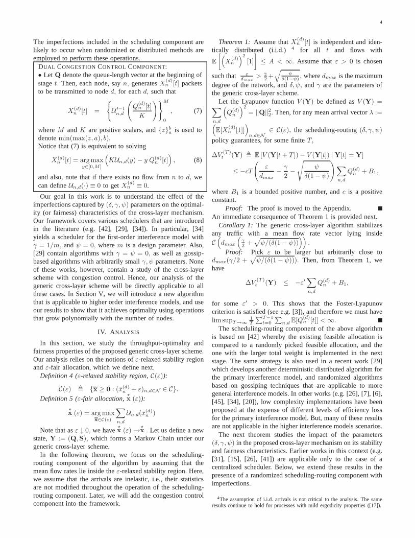
The schedule used for packet transmissions is updatedat the beginning of each stage. Throughout a stage, packettransmissions are performed according to the schedule updatedat the beginning of that stage. In parallel with the packettransmissions, PICK and COMPARE algorithms are imple-mented. Since the same medium is shared, the data packettransmissions can collide with the control messages generatedby these algorithms. To prevent such collisions, time is dividedinto two intervals, namely thecontrol signalling interval(CSI)during which control messages are locally communicated,and thedata transmission interval(DTI) during which datapackets are transferred (see Figure 1). Notice that both PICK

and COMPARE algorithms operate during CSI, while queue-lengths are updated during DTI. It is assumed that all thenodes are synchronized to the same CSI/DTI division of time.This assumption can be relaxed by adding a buffer intervalbetween CSI and DTI to accommodate propagation delays.Alternatively, the control signalling can be performed overan orthogonal channel through frequency division. Finally,we assume that each transceiver can perform carrier sensingduring transmission without the need to decode its reception5.

It is important to note that in our algorithm the overheadintroduced by the control signalling can be made arbitrarily

5This assumption is not critical, but simplifies the PICK algorithm descrip-tion and analysis. When it is relaxed, the first step of the algorithm need tobe modified to let each transceiver transmit randomly to a random neighborwithout sending a previous RTS.

7

Fig. 1. Division of time into data transmission and control signallingintervals.

small by increasing the length of a stage to a high enoughvalue. This fact follows from thefixedamount of control mes-sages required by our algorithmper stage. Thus, the numberof control messages versus the data messages in a stage canbe made negligible by increasing the stage duration. This willnaturally result in slower convergence, but the stability andfairness results of Theorem 2 will continue to hold.

We assume that each node has a unique ID number pickedfrom a totally ordered set. LetID(n) denote the ID numberof noden. Then, unique ID numbers can be assigned to links,denoted byID(n,m) = ID(m,n) for link (n,m). Thisassumption is essential for each node (and link) to identifyits neighboring nodes (and links), and will be used in thedistributed implementation of our algorithms.

A. PICK Algorithm

In this section, we present a distributed algorithm thatrandomly picks a feasible allocationR with the property thatany feasible allocation has a positive probability of beingchosen as required by (5). In the description of the algorithm,when we say a nodewithdraws, we mean that the node stopsits search for a feasible link during the current stage, butcontinues to listen to other transmissions. The algorithm makessure that each node has a positive probability of attemptingtransmission at the beginning of the algorithm. The idea is tosend Ready-to-Send (RTS) and Clear-to-Send (CTS) packetsincluding the ID numbers of the nodes in order to create afeasible allocation. By appending ID numbers to the RTS/CTSpackets, the algorithm enables each node to have a list ofthose links in its local neighborhood that are picked by thealgorithm.

Definition 6 (PICK Algorithm): At every noden ∈ N per-form the following steps:

(A1) In step 1, with probability pn ∈ [α, 1) for someα ∈ (0, 1), n transmits a (RTS) message.

(A1a) If n senses another transmission during its (RTS)transmission, it withdraws.

(A2a) If n does not sense another transmission, in step2,it chooses one of its neighbors, saym, randomly with equalprobabilities, and transmits (RTS,ID(m)).

(A2b) If m observes a collision, it withdraws.(A3a) If m getsn’s message, in step3, it sends back a

(CTS) message.(A3b) If m senses another transmission during its (CTS)

transmission, it withdraws.(A3c) If n observes an idle, it withdraws.(A4a) If m does not sense another transmission during its

(CTS) transmission, in step4, it transmits (CTS,ID(n,m)).(A4b) If n does not receivem’s response, it withdraws.

(A5) In step5, n transmits (CTS,ID(n,m)), and the linkbetweenn andm is activated; link(n,m) is added toR. ⋄

The algorithm assures between steps (A1) and (A2a), thatno two transmitters are neighboring each other; at (A2b), thatno transmitter is a neighbor to a receiver; between (A3a) and(A4a), that no two receivers are neighbors. Finally, during(A4a) and (A5), the picked link is announced to the neighborsof the receiver and the transmitter, respectively.

Notice that the algorithm need not result in amaximalfeasible allocation6 at its termination. This does not influencethe results of Theorem 2, but will have an effect on the rate ofconvergence of the algorithm. With a simple modification, theabove algorithm can be extended to obtain a maximal feasibleallocation and hence better convergence properties.

Proposition 1: The above PICK algorithm satisfies(i) The resultingR is a feasible allocation.(ii) It takes at most5 transmissions per node to terminate.(iii) The probability of picking any feasible allocation is

at least (min(α, 1 − α)/dmax)N

> 0, where dmax is the

maximum degree7 of G. In particular, since⋆

SW [t] is a

feasible schedule, we haveP(R[t] =⋆

SW [t]) ≥ (min(α, 1 −α)/dmax)

N > 0.(iv) At the termination, for any link(n,m) ∈ L, all the

neighbors ofn andm are aware of(n,m)’s state, i.e., knowwhether(n,m) is in R or not.

Proof: Step (A1a) assures that if two neighboring nodesattempt to transmit, they sense each other and withdraw. InStep (A2b), the event that more than one neighbors of anode are attempting to transmit is detected, and in that eventall of the transmitters withdraw from transmission in Step(A3c). Finally, step (A3b) guarantees that two neighbors donot become receiving ends of two different links. Thus, all theevents that leads to interfering links are eliminated in thesesteps, and the resulting allocation must be feasible, whichproves (i). Claim(ii) follows immediately from the constructionof the algorithm.

To prove Claim(iii), note that if the initially picked set oflinks in steps (A1) and (A2a) happen to be feasible, they arenot eliminated throughout the algorithm, because the algorithmis designed to eliminate only those links that interfere witheach other. Thus, we are interested in finding a lower boundon the probability of picking a given feasible schedule, sayW ∈ S, at the start. Thus, we need to have exactly|W |nodes, one from each link inW choose to transmit in step (A1)(which happens with probabilityα|W |), and all the remainingnodes must be silent (which happens with probability≥ (1−α)N−|W |). If each of those nodes which chose to transmit,picks its outgoing link that lies inW for transmission instep (A2a) (which happens with probability≥ (α/dmax)

|W |),then the resulting schedule will be exactlyW. Hence, theprobability that PICK yields a given feasible scheduleW is≥ (α/dmax)

|W |(1 − α)N−|W | ≥ (min(α, 1 − α)/dmax)N ,

where the last step follows fromdmax ≥ 1.

6A maximal feasible allocation is a set of links to which no new link thatdoes not interfere with any of the existing links can be added.

7deg(n) , |{m ∈ N : (n, m) ∈ L, or (m, n) ∈ L}|.

8

Claim(iv) follows from the fact that the links that areactivated are announced to neighboring nodes via the message(CTS, ID(n,m)), and therefore all the neighbors know theIDs of the activated links in their two hop neighborhood.

We note that this algorithm does not depend on the queue-lengths, which greatly simplifies its implementation, becauseno queue-length information exchange is necessary betweenneighboring nodes. Further, due to part (iii), the best allocationmust also have a positive probability. This fact together withparts (i)-(iii) prove that the algorithm is actually sufficient forTheorem 2 to hold. At the end of PICK, R gives a feasibleallocation, that is known only locally. In particular, due topart (iv) of Proposition 1, every node knows those links of itsneighbors that are inR.

B. COMPARE Algorithm

In this section, we propose and analyze a distributed al-gorithm that compares the total weight associated with twofeasible schedules,S[t] and R[t], with local control signaltransmissions, and choose the one with the larger weight asthe schedule to be used during the next stage. We note thatthis algorithm also applies to interference models other thanthe secondary interference model. In the following, we willomit the time index for ease of presentation.

The algorithm relies on constructing theconflict graphassociated withS and R which contains information aboutinterfering links in the two schedules. The conflict graph,G′(S,R) = (N ′,L′), of S and R can be generated asfollows8: Each link l in S ∪ R corresponds to a node in theconflict graph, and if linksl1 ∈ S and l2 ∈ R interfere witheach other, an edge is drawn between the nodes correspondingto l1 and l2 in the conflict graph. Note that, since bothS andR are feasible schedules, no two links in the same schedule(S or R) can interfere with each other, i.e., there is no edgebetween two nodes of the same schedule inG′. Every node inG′ can compute its own weight [as defined in (3)], and has alist of its neighbors inG′ by part (iv) of Proposition 1. We willdevelop the algorithms using the conflict graphG′ and showat the end of this section that the special structure enablesusto map the operations to the graphG.

Our COMPARE Algorithm is composed of two proceduresthat are implemented consecutively: FIND SPANNING TREE

and COMMUNICATE & D ECIDE. The FIND SPANNING TREE

procedure finds a spanning tree for each connected componentof G′ in a distributed fashion. Then, the COMMUNICATE &DECIDE procedure exploits the constructed tree structure tocommunicate and compare the weights of the two schedulesin a distributed manner.

To illustrate the definitions and operation of the algorithmswe consider the grid network depicted in Figure 2. In thisnetwork, nodes are located on the corner points of a grid, andeach interior node has four links incident to it. To demonstratethe construction of the conflict graph, suppose we are giventwo feasible schedules,S andR. In the figure, solid bold linksbelong to scheduleS, while dashed bold links are inR.We use

8We useN ′, L′ to denote the cardinalities ofN ′,L′. Also, we will referto G′(S, R) simply asG′ for convenience.

����

����

����

����

����

����

����

����

����

����

����

����

����

����

����

����

����

����

����

����

����

����

����

����

����

����

����

����

����

����

����

����

����

����

����

����

����

����

����

����

����

����

����

����

����

����

����

����

����

����

����

����

����

����

����

����

����

����

����

����

����

����

����

����

����

����

����

����

����

����

����

����

����

����

����

����

����

����

����

����

�����������

�����������

������������

������������

�����������

�����������

������������ ������������

Fig. 2. 8x10 grid network example with two feasible schedules indicatedby solid and dashed bold links. The conflict graph decomposesinto 6disconnected components.

dash-dotted thin lines to connect the links of the two schedulesthat interfere with each other. In general, it is not necessarythat the conflict graph be connected. For example, in Figure 2,we observe six disconnected components. The conflict graphcorresponding to the largest connected component is given inFigure 3, where links inS are drawn as circular dots, whilelinks in R are drawn as square dots.

Remark 1:Disconnected components of the conflict graphcan decide on which schedule to use, independent of eachother. This is possible because by construction of the conflictgraph the resulting schedule is guaranteed to be feasible evenif the choices of two disconnected components are different.This decomposition contributes to the distributed nature ofthe algorithm. Namely, the size of the graph within whichthe comparison is to be performed is likely to be reduced.Notice that with this approach, the chosen schedule may bea combination of the two candidate schedules,S and R,because different connected components may prefer differentschedules. This merging operation will result in a schedulethat is better than bothS andR.

Based on this remark, henceforth our algorithm will focuson the decision of a single connected component.

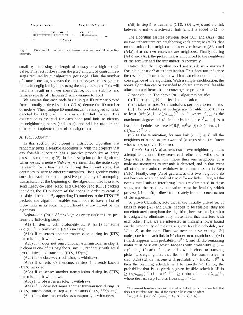
1) FIND SPANNING TREE Procedure: The object of theFIND SPANNING TREE procedure is to find, in a distributedfashion, a spanning tree for each of the connected componentsin the conflict graph. In our model, every node in the conflictgraph G′ corresponds to an undirected link in the originalgraphG, and has a unique ID9. In order to compare two linkIDs, we use lexicographical ordering10.

Our distributed FIND SPANNING TREE procedure is basedon token generation and forwarding operations. For the con-struction of a spanning tree, at least one token needs to begenerated within each connected component. This can beguaranteed by requiring every node in the conflict graph thathas the lowest ID number among its neighbors to generate atoken. Each token, carrying the ID of its generator, performs adepth-first traversal (cf. [9]) within the connected component

9In [18], it was shown that unique IDs are required to be able tofind aspanning tree in a distributed fashion.

10Without loss of generality, assumeID(n) < ID(m) and ID(i) <ID(j) : If ID(n) < ID(i), then ID(n, m) < ID(i, j) for all m, j; andif ID(n) = ID(i) andID(m) < ID(j), thenID(n, m) < ID(i, j).

9

to construct a spanning tree. This token progressively addsnodes into its spanning tree while avoiding the constructionof cycles. An example is depicted in Figure 3 for the largestconnected component of Figure 2.

������������

������������

������

������

��������

��������

������

������

������

������

X

tokenminimum

6

3

10

5

24

7 8

11

9

12

1

Fig. 3. A connected component of the conflict graph from whichthe linkcrossed is eliminated to obtain a spanning tree. The path of the minimumtoken is indicated with arrows. The nodes are labeled with numbers for futurereference.

The above procedure focuses on the operation of a singletoken generated at one of the nodes within the connectedcomponent. In general, there may be multiple tokens generatedwithin the same connected component. Each token attempts toform its spanning tree labeled with its ID number (i.e. the IDnumber of the token’s generator). Since only one spanningtree is required at the end of the procedure, our algorithmis designed to keep the spanning tree with the smallest IDnumber, while eliminating the others. This elimination isperformed when the token of a spanning tree enters a node thathas already been traversed by another token. If the incomingtoken has smaller ID, then the token ignores the previous tokenand continues the construction of its tree, and if its ID islarger, then it is immediately deleted. We have the followingproposition for this algorithm.

Proposition 2: Consider the conflict graphG′ = (N ′,L′),and letd′max denote the maximum degree ofG′. The FIND

SPANNING TREE Procedure finds a spanning tree of allcomponents of the conflict graph inO(d′maxL

′) time11, andwith O(d′maxN

′) message exchanges for eachn′ ∈ N ′. Also,at the termination of the procedure, every noden′ ∈ N ′ hasa list of its neighbors in the constructed spanning tree.

Proof: To prove that the constructed subgraph by thesmallest token is in fact a spanning tree, we need to show thatevery node is in the formed subgraph, and that the subgraphcontains no cycles. To argue that every node must be in thesubgraph, let us assume, to arrive at a contradiction, thereis anode, sayz′ ∈ N ′, that is not in the subgraph but is within theconnected component. If any ofz′’s neighbors had held thetoken at any time, then it must have attempted to forward thetoken toz′ before it sends the token back to its parent. But,if a token attempt is made toz′, it will ACCEPT it because itis the first time it encounters such an attempt. This argumentimplies that none of the neighbors ofz′ can be in the subgraph.

11f(n) = O(g(n)) means that there exists a constantc < ∞ such thatf(n) ≤ cg(n) for n large enough.

If the same arguments are made repeatedly, this implies thatthe whole subgraph must be empty. But, we know that the nodethat generates the token is in the subgraph by default. Hence,we get a contradiction, and the subgraph must contain everynode within the connected component. The argument that thesubgraph contains no cycles follows from the fact that everynode ACCEPTs only those token transmissions that do notform a cycle. Thus, the resulting subgraph must be acyclic.

The procedure is constructed so that whenever a tokenwith a larger ID crosses any node of the spanning tree beingconstructed by a token with a smaller ID, the token withthe larger ID along with its spanning tree is eliminated. Bydefinition, a spanning tree has to contain every node and thusall the tokens must meet with the spanning tree of the smallesttoken sometime. Therefore, by the end of the procedure, onlythe spanning tree of the smallest token survives.

To compute the complexity, we take into account the com-plexity of resolving potential collisions of tokens. It is not diffi-cult to see that each such collision can be resolved inO(d′max)message exchanges. Since, an operation ofO(d′max) opera-tions must be performed for2L′ times, we needO(d′maxL

′)time for the operation to complete. However, each node willonly transmitO(d′max) messages in the process only whenit is receiving and transmitting a token. Since, there are atmostO(N ′) tokens in the system, the number of messagestransmitted by each node isO(d′maxN

′).We note that the FIND SPANNING TREE procedure that we

described here is deterministic and achievesγ = 0 in thecontext of the generic cross-layer scheme of Definition 3.Alternatively, a randomized gossip style mechanism can beused that yieldsγ > 0 (see [30]). Theorem 2 can be used tounderstand the fairness characteristics of both approaches.

2) COMMUNICATE & D ECIDE Procedure: We use thespanning tree formed on the conflict graph to compare weights.The idea is to convey the necessary information from theleaves up to the root of the tree (i.e. COMMUNICATE Proce-dure) so that the schedule with the higher weight is chosen (cf.(6)), and then send back the decision to the leaves (i.e. DECIDE

Procedure). The COMMUNICATE & D ECIDE procedure can beexplained in two parts as follows:

COMMUNICATE : The leaves communicate their weights totheir parents. If the parent is inS it adds its weight to the sumof the weights announced by its children. If, on the other hand,it is in R it subtracts its weight from the sum of its children’sweights. The resulting value becomes the new weight of theparent. Then, the parent acts as a leaf with the updated weightin the next iteration. This recursive update is repeated untilthe root is reached.

DECIDE: At the end of COMMUNICATE, the weight ofthe root of the spanning tree will be

∑

l∈Swl −

∑

l∈Rwl.

Depending on whether the root’s weight is positive or negative,the root decidesS or R, respectively, as the better schedule,and broadcasts its decision down the tree.

An example of this procedure is provided in Figure 4 forthe spanning tree given in Figure 3. We have the followingcomplexity result for this procedure.

Proposition 3: Consider the conflict graphG′ = (N ′,L′),and letd′max denote the maximum degree ofG′. The COM-

10

Fig. 4. The iterative communication of the weights of the twoschedulesfrom the leaves to the root for the spanning tree of Figure 3.

MUNICATE & D ECIDE procedure correctly finds the schedulewith the larger weight inO(d′maxL

′) time.Proof: The algorithm is designed so that when noden′

transmits its current sum to its parent, the value of the sum isthe difference of the weights of scheduleS andR only for thesubtree rooted atn′. Thus, the sum at the root of the spanningtree is the difference of two weights of scheduleS andR. Thedecision is a simple comparison of the sign of this sum. Thisdecision is broadcast to the children of the root, and hence allthe nodes in the connected component knows about the betterschedule and can switch to it by the end of the procedure.The depth of the spanning tree can be at mostO(L′) and eachcollision resolution operation can take at mostO(d′max) time.Thus, the whole algorithm terminates inO(L′d′max) time.

Notice that the complexity results in the propositions aregiven in terms ofG′. We can translate them into bounds onG through the following inequalities:L′ < N2, d′max < N .Thus, combining Propositions 1-3 with Theorem 2 yields:

Theorem 3:The distributed implementations of PICK andCOMPARE Algorithms designed for the secondary interferencemodel asymptotically achieve throughput-optimality and fair-ness withO(N3) time andO(N2) message exchanges pernode, per stage. �

We conclude the section with a few important remarks.Remark 2:The algorithms we develop in this section oper-

ate over the conflict graphG′. The transformation of theseoperations into operations in the actual graphG would bedifficult for a general conflict graph. However, in our scenariothe graph has a special structure that enables the mapping.The critical observation is that transmissions within a feasibleschedule has no interference. Thus, links that formS andR can perform operations inG′ by partitioning CSI (cf.Figure 1) into two disjoint time intervals. During the firstinterval, only links that make upS communicate, while in thesecond interval only nodes that make upR communicate. Theoperation of each link can easily be mapped into operationsat its two end nodes by assigning one node to each operation,who will then coordinate the operation. With such a separationof time, the operations described for the conflict graph can betranslated into operations in the actual network.

Remark 3:Recall from Remark 1 that the conflict graph is

likely to be composed of multiple disconnected components,which increases the distributed nature of the algorithms. Eventhough we did not pursue this direction here, this likelihoodcan be increased by dynamically modifying the activationprobabilities,{pn}n, in the PICK Algorithm so that the pickedschedule has more disconnected components. This way, thelocalized nature of the algorithm can be improved.

VI. SIMULATIONS

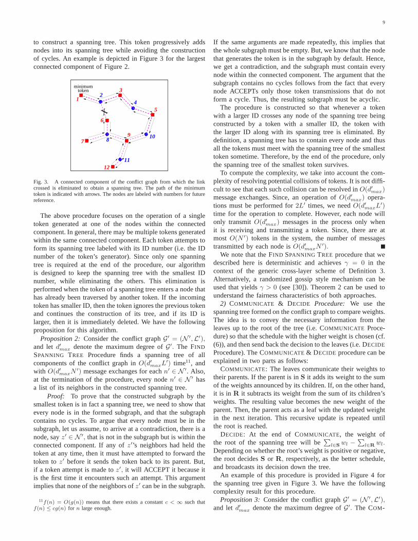
In this section, we provide simulation results for thedistributed algorithms developed in Section V for the gridtopology (see Figure 2). We use the notation[i, j] to refer tothe node at theith row andjth column of the grid. Throughout,we simulate utility functions of the formUi(x) = γi log(x),which corresponds to weighted proportionally fair allocation(see [23], [40]).

0 1 2 3 4 5 6 7 8 9 10

x 104

0

0.05

0.1

0.15

0.2

0.25

Throughput evolution for 6x6 Network with 4 flows

Number of Stages

Thr

ough

put a

chie

ved

Flow−1Flow−2Flow−3Flow−4

Fig. 5. The throughput evolution of the 6x6 network forK = 100, γi = 0.5.

We first consider a network of size 6x6, with four flows:Flow-1 from [1, 1] to [6, 6], Flow-2 from [5, 2] to [6, 3], Flow-3 from [5, 5] to [5, 1], and Flow-4 from [4, 1] to [1, 4]. Here,we are interested in the evolution of the throughputs of eachflow for K = 100 and γi = 0.5 for each i ∈ {1, 2, 3, 4}.The simulation results are depicted in Figure 5. We observethat the throughputs of the flows converge to different valuesdepending on their source-destination separation. For example,Flow-2 achieves the highest throughput since its source isonly two hops from its destination. The fluctuations in theevolutions are due to the random nature of the algorithm,which tracks the queue-length evolutions.

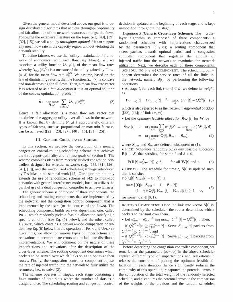
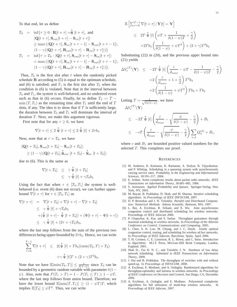
Next, we simulate a 10x10 network with two flows: Flow-1from [1, 1] to [8, 9], and Flow-2 from [9, 2] to [2, 10]. Here, wefocus on the throughputs achieved for the flows as a functionof K with varying γi for each flow. We aim to observe themean flow rates as functions ofK and (γ1, γ2). Notice thateach(γ1, γ2) combination corresponds to a different weightingfor the weighted-proportionally fair allocation. Thus, for afixed K, the throughputs corresponding to different(γ1, γ2)combinations actually outline therate regionthat the algorithmachieves for thatK. Then, asK grows Theorem 2 implies thatthis region grows at a decreasing rate, until it converges tothestability regionC.

We performed simulations forK varying from 10 to 100,and(γ1, γ2) ranging from(0, 1) to (1, 0) with γ1 + γ2 = 1 at

11

0 0.05 0.1 0.15 0.2 0.25 0.3 0.35 0.4 0.450

0.05

0.1

0.15

0.2

0.25

0.3

0.35

0.4

Throughput of Flow−1

Tho

ughp

ut o

f Flo

w−2

K=10 K=20 K=40 K=60 K=80

K=100

(0,1) (.1,.9) (.2,.8)

(.3,.7)

(.4,.6)

(.5,.5)

(.6,.4)

(.7,.3)

(.8,.2)

(.9,.1)

(γ1,γ

2)

Fig. 6. Throughputs of flows with varyingK and (γ1, γ2).

each intermediate point. The simulation results are providedin Figure 6. We observe that for a givenK, the rate regionis a convex region. Also, asK grows, the region expands ata decreasing rate agreeing with our expectations. We furthernote that with this algorithmic method, the stability region ofa wireless network, that is otherwise difficult to find, can bedetermined with high accuracy.

While our work focuses on optimizing the long-term net-work utilization metric, we note that, for many applications,delay is just as important a metric to optimize. We note thatthe interference-limited nature of the medium along with therandomized implementations are causes of delay degradations.Our simple, randomized algorithm is quite general, and isoblivious to network structure and scheduling constraints. Anylow-complexity algorithm with such generality is unlikelyto achieve low delay [10]. Yet, there is potential for delayperformance improvements, which constitutes the motivationfor our ongoing works in this direction.

VII. C ONCLUSIONS

We provided a framework for the design of distributedcross-layer algorithms for full utilization of multi-hop wirelessnetworks. To that end, we first described a generic scheduling-routing-congestion control mechanism that allows for variousimperfections and relaxations in its operation which facilitatesthe design of distributed implementations. We studied thestability and fairness characteristics of the generic cross-layeralgorithm, and explicitly characterized the effect of differenttype of imperfections on its performance. We saw that certaintypes of imperfections are more detrimental than others, whichrevealed the critical components in the design of algorithms.

Based on this foundation, we developed specific distributedalgorithms for the secondary interference model. For thismodel, existing throughput-optimal strategies require that anNP-hard problem be solved by a centralized controller at everytime instant. In this work, we showed that this is not necessary,and full utilization of the network can be achieved withdistributed algorithms having only polynomial communicationand computational complexity.

An important byproduct of our approach is the use of thedeveloped cross-layer algorithms to find (with high accuracy)the stability region of ad-hoc wireless networks, that areotherwise difficult to characterize.

APPENDIX

We defined the notion of capacity (stability) region inDefinition 2. A characterization of this region in terms offlow conservation and feasibility constraints is provided byTassiulas and Ephremides in their seminal work [43], whichis reproduced in the following proposition to be used in theproof of Theorem 1.

Proposition 4: Let G = (N ,L) be a given network andSbe the set of feasible allocations. The capacity (or stability)region C of the network is given by the set of vectorsr =

(r(d)n )n,d∈N for which there existsz(d)

(n,m) ≥ 0 for all (n,m) ∈L andd ∈ N , such that both the flow conservation constraintsat the nodes and the feasibility constraints are satisfied, i.e.,

(C1) For alln ∈ N andd ∈ N\{n}, we have

r(d)n +∑

k:(k,n)∈L

z(d)(k,n) =

∑

m:(n,m)∈L

z(d)(n,m),

(C2)

[

∑

d∈N

(

z(d)(n,m) + z

(d)(m,n)

)

]

(n,m)∈L

∈ Conv(S). 12

Proof of Theorem 1:

Before the start the proof, we note that it closely followsthe technique of [29], except that it is extended to multi-hop flows and more general arrival processes. The multi-hop extension adds a routing component to the mechanismand add some technical complications to the proof. Moreimportantly, in this work we further include congestion control(cf. Theorem 2) into the framework of [29] to investigatethe fairness characteristics of the joint congestion control,scheduling and routing mechanism.

We first derive an upper bound on the single-step mean driftof the Lyapunov function,∆V (1)

t (Y), for a givenY = (Q,S).

∆V(1)t (Y)

= E[

‖Q[t+ 1]‖22 − ‖Q[t]‖2

2 |Y[t]]

≤∑

n,d

E

[(

(

Q(d)n [t] − S

(d)out(n)[t]

)+

+X(d)n [t]

+S(d)in(n)[t]

)2

− (Q(d)n [t])2 |Y[t]

]

=∑

n,d

E

[(

Q(d)n [t] − S

(d)out(n)[t] + U

(d)out(n)[t] +X(d)

n [t]

+S(d)in(n)[t]

)2

− (Q(d)n [t])2 |Y[t]

]

=∑

n,d

E

[(

Q(d)n [t] − S

(d)out(n)[t] +X(d)

n [t]

+S(d)in(n)[t]

)2

− (Q(d)n [t])2 |Y[t]

]

(16)

+∑

n,d

2E

[

U(d)out(n)[t]

(

Q(d)n [t] − S

(d)out(n)[t] +X(d)

n [t]

+S(d)in(n)[t]

)

+(

U(d)out(n)[t]

)2

|Y[t]

]

(17)

12Conv(A) denotes the convex hull of setA, which is the smallest convexset that includesA. The convex hull is included in view of the possibility oftimesharing between feasible allocations.

12

whereU (d)out(n)[t] denotes the amount of unused service by node

n to transmit packets of typed in slot t. Note thatU (d)out(n)[t]

can be non-zero only whenQ(d)n [t] is low. Also, since the

service rate over each link is upper-bounded by one,U(d)out(n)[t]

must also be upper-bounded by the maximum degreedmax ofthe network. First, we show that (17) is upper-bounded.

(17) ≤∑

n,d

(

2E

[

U(d)out(n)[t]Q

(d)n [t] | Y[t]

]

+4dmax + 2λ(d)n + d2

max

)

≤ N2(3d2max + 6dmax) =: b1,

where, in the last step, we used the fact thatU(d)out(n)[t] ≤ dmax

and thatλ(d)n ≤ dmax.

Next, we study (16). We can re-write it in inner-productform after cancelations

(16) = 2E [〈 Q[t],Sin[t] + X[t] − Sout[t]〉+‖Sin[t] + X[t] − Sout[t]‖2

2 | Y[t]]

≤ 2E [〈 Q[t],Sin[t] + X[t] − Sout[t]〉 |Y[t]] + b2, (18)

whereb2 is a finite constant since: the service rate into or outof any node is bounded bydmax; and the second moment ofthe arrival process is assumed to be bounded.

Next, we study the expectation in (18) in further detail.We omit the the time index[t] in the following derivation fornotational convenience.

E [〈 Q,Sin + X − Sout〉 | Y] = 〈 Q,⋆

Sin +λ−⋆

Sout〉+〈Q,Sin−

⋆

Sin −Sout+⋆

Sout〉(19)

where⋆

SW is chosen according to (4). Sinceλ ∈ C(ε),Proposition 4 implies that there exists a non-

negative vector S =(

S(d)(n,m)

)d∈N

(n,m)∈Lsuch that:

[

∑

d∈N

(

S(d)(n,m) + S

(d)(m,n)

)

]

(n,m)∈L

∈ Conv(S); and

λ(d)n + S

(d)in(n) = S

(d)out(n) − ε, ∀n, d 6= n,

which can be written compactly asλ = Sout − Sin − ε1 invector form, where1 is a vector of all ones. Substituting thisinto the first inner product in (19) yields.

〈 Q,⋆

Sin +λ−⋆

Sout〉 = 〈 Q, Sout − Sin〉−〈Q,

⋆

Sout −⋆

Sin〉 − ε〈 Q,1〉

Note that

〈 Q,⋆

Sout −⋆

Sin〉 =∑

n,d

Q(d)n

(

⋆

S(d)

out(n) −⋆

S(d)

in(n)

)

=∑

(n,m)∈L

∑

d

⋆

S(d)

(n,m)

(

Q(d)n −Q(d)

m

)

=∑

(n,m)∈L

⋆

S(n,m) maxd

∣

∣

∣Q(d)n −Q(d)

m

∣

∣

∣

(a)

≥∑

(n,m)∈L

S(n,m) maxd

∣

∣

∣Q(d)n −Q(d)

m

∣

∣

∣

≥∑

(n,m)∈L

∑

d

S(d)(n,m)

(

Q(d)n −Q(d)

m

)

= 〈Q, Sout − Sin〉,

where the inequality(a) follows from (4). Substituting this inthe previous expression yields

〈 Q,⋆

Sin +λ−⋆

Sout〉 ≤ −ε〈Q,1〉≤ − ε

dmax〈 Q,

⋆

Sout −⋆

Sin〉,

where the last inequality follows from the fact that⋆

Sout(n)

−⋆

Sin(n)≤ dmax for all n. We substitute this upper bound in(19) with the new notation:Ψ[t] := 〈 Q[t],Sout[t] − Sin[t]〉,and

⋆

Ψ [t] := 〈 Q[t],⋆

Sout [t]−⋆

Sin [t]〉, and Ψ[t] :=〈 Q[t],Rout[t] − Rin[t]〉.

E [〈 Q[t],Sin[t] + X[t] − Sout[t]〉 |Y[t] = Y]

≤ − ε

dmax

⋆

Ψ [t]+⋆

Ψ [t] − Ψ[t]

We use this bound in (18) and bound theT -step mean drift as∆V

(T )t (Y)

≤ −2ε

dmax

T−1∑

τ=0

E[⋆

Ψ [t+ τ ] |Y[t] = Y] + Tb2 (20)

+

T−1∑

τ=0

E[⋆

Ψ [t+ τ ] − Ψ[t+ τ ] |Y[t] = Y] (21)

To bound (20) note that

T−1∑

τ=0

E[⋆

Ψ [t+ τ ] |Y[t] = Y] ≥T−1∑

τ=0

(

⋆

Ψ [t] − τb3

)

≥ T⋆

Ψ [t] − T 2

2b3, (22)

where the first inequality follows from the fact that in a singletime slot, each queue can change by at most a bounded value,and therefore there exists a constantb3, such that

|⋆

Ψ [τ + 1]−⋆

Ψ [τ ]| ≤ b3 for any τ.Next, we are interested in upper-bounding (21). For nota-

tional convenience, let us define∇[t] :=⋆

Ψ [t]−Ψ[t]. Hence, weare interested in upper-bounding

∑T−1τ=0 E[∇[t+τ ]|Y[t] = Y].

13

To that end, let us define

T0 = inf{τ ≥ 0 : R[t+ τ ] =⋆

S [t+ τ ], and

〈Q[t+ τ ],Sout[t+ τ ] − Sin[t+ τ ]〉≥ max (〈Q[t+ τ ],Sin[t+ τ − 1] − Sout[t+ τ − 1]〉,(1 − γ)〈Q[t+ τ ],Rout[t+ τ ] − Rin[t+ τ ]〉)}

T1 = inf{τ > T0 : 〈Q[t+ τ ],Sout[t+ τ ] − Sin[t+ τ ]〉< max (〈Q[t+ τ ],Sin[t+ τ − 1] − Sout[t+ τ − 1]〉,(1 − γ)〈Q[t+ τ ],Rout[t+ τ ] − Rin[t+ τ ]〉)}.

Thus,T0 is the first slot aftert when the randomly pickedscheduleR according to (5) is equal to the optimum schedule,and (6) is satisfied; andT1 is the first slot afterT0 when thecondition in (6) is violated. Note that in the interval betweenT0 andT1, the system is well-behaved, and no undesired eventsuch as that in (6) occurs. Finally, let us defineT2 := T −min (T, T1) as the remaining time afterT1 until the end ofTslots, if any. The idea is to show that ifT is sufficiently large,the duration betweenT0 andT1 will dominate the interval ofdurationT. Next, we make this argument rigorous.

First note that for anyτ ≥ 0, we have

∇[t+ τ ] ≤ 2⋆

Ψ [t+ τ ] ≤ 2⋆

Ψ [t] + 2τb3.

Next, note that atτ = T0, we have

〈Q[t+ T0],Sout[t+ T0] − Sin[t+ T0]〉≥ (1 − γ)〈Q[t+ T0],

⋆

Sout [t+ T0]−⋆

Sin [t+ T0]〉

due to (6). This is the same as

∇[t+ T0] ≤ γ⋆

Ψ [t+ T0]

≤ γ⋆

Ψ [t] + γT0b3

Using the fact that whenτ ∈ [T0, T1] the system is well-behaved (i.e. event (6) does not occur), we can further upper-bound∇[t+ τ ] for τ ∈ [T0, T1] as

∇[t+ τ ] = ∇[t+ T0] + ∇[t+ τ ] −∇[t+ T0]

≤ γ⋆

Ψ [t] + γT0b3

+(⋆

Ψ [t+ τ ]−⋆

Ψ [t+ T0]) + (Ψ[t+ τ ] − Ψ[t+ τ ])

≤ γ⋆

Ψ [t] + (2τ + γT0)b3,

where the last step follows from the sum of the previous twodifferences being upper-bounded by2τb3. Hence, we can write

T−1∑

τ=0

∇[t+ τ ] ≤ 2(⋆

Ψ [t] + Tb3)(min(T0, T ) + T2)

+γ⋆

Ψ [t]T + (2 + γ)T 2b3.

Note that we haveE[min(T0, T )] ≤ 1δ(1−ψ) sinceT0 can be

bounded by a geometric random variable with parameterδ(1−ψ). Also, note thatP (T1 > T ) = 1 − P (T1 ≤ T ) ≥ 1 − ψT,where the last step follows from union bound. Therefore, wehave the lower boundE[min(T, T1)] ≥ (1 − ψT )T, whichimplies E[T2] ≤ ψT 2. Thus, we can write

E

[

∑T−1τ=0 ∇[t+ τ ] |Y[t] = Y

]

≤ 2T⋆

Ψ [t]

(

ψT +1

δ(1 − ψ)T+γ

2

)

+2Tb3

(

1

δ(1 − ψ)+ ψT 2

)

+ (2 + γ)T 2b3

Substituting (22) in (20), and the previous upper bound into(21) yields

∆V(T )t (Y) ≤ −2T

⋆

Ψ [t]

(

ε

dmax− ψT − 1

δ(1 − ψ)T− γ

2

)

+2

(

ε

dmax+ 1 +

γ

2

)

T 2b3

+2

(

1

δ(1 − ψ)+ ψT 2

)

Tb3 + Tb2

Letting T = 1√δψ(1−ψ)

, we have

∆V(T )t (Y)

≤ −2T⋆

Ψ [t]

(

ε

dmax−√

ψ

δ(1 − ψ)− γ

2

)

+B1

≤ −cT(

ε

dmax−√

ψ

δ(1 − ψ)− γ

2

)

∑

n,d

Q(d)n +B1,

wherec andB1 are bounded positive valued numbers for theselectedT. This completes our proof.

REFERENCES

[1] M. Andrews, K. Kumaran, K. Ramanan, A. Stolyar, R. Vijayakumar,and P. Whiting. Scheduling in a queueing system with asynchronouslyvarying service rates.Probability in the Engineering and InformationalSciences, 18:191–217, 2004.

[2] E. Arikan. Some complexity results about packet radio networks. IEEETransactions on Information Theory, 30:681–685, 1984.

[3] S. Asmussen.Applied Probability and Queues. Springer-Verlag, NewYork, NY, 2003.

[4] M. Bayati, B. Prabhakar, D. Shah, and M. Sharma. Iterative schedulingalgorithms. InProceedings of IEEE INFOCOM, 2007.

[5] D. P. Bertsekas and J. N. Tsitsiklis.Parallel and Distributed Computa-tion: Numerical Methods. Athena Scientific, Belmont, MA, 1997.

[6] L. Bui, A. Eryilmaz, R. Srikant, and X. Wu. Joint asynchronouscongestion control and distributed scheduling for wireless networks.Proceedings of IEEE Infocom 2006.

[7] P. Chaporkar, K. Kar, and S. Sarkar. Throughput guarantees throughmaximal scheduling in wireless networks. InProceedings of the AllertonConference on Control, Communications and Computing, 2005.

[8] L. Chen, S. H. Low, M. Chiang, and J. C. Doyle. Jointly optimalcongestion control, routing, and scheduling for wireless ad hoc networks.In Proceedings of IEEE Infocom, Barcelona, Spain, April 2006.

[9] T. H. Cormen, C. E. Leiserson, R. L. Rivest, and C. Stein.Introductionto Algorithms. M.I.T. Press, McGraw-Hill Book Company, London,England, 2001.

[10] Shah D., Tse D. N. C., and Tsitsiklis J. N. Hardness of lowdelaynetwork scheduling.Submitted to IEEE Transactions on InformationTheory, 2009.

[11] J. Dai and B. Prabhakar. The throughput of switches withand withoutspeed-up. InProceedings of INFOCOM, 2000.

[12] A. Eryilmaz, E. Modiano, and A. Ozdaglar. Randomized algorithms forthroughput-optimality and fairness in wireless networks.In Proceedingsof IEEE Conference on Decision and Control, San Diego, CA, December2006.

[13] A. Eryilmaz, A. Ozdaglar, and E. Modiano. Polynomial complexityalgorithms for full utilization of multi-hop wireless networks. InProceedings of IEEE Infocom, 2007.

14

[14] A. Eryilmaz, A. Ozdaglar, D. Shah, and E. Modiano. Imperfectrandomized algorithms for the optimal control of wireless networks.In Proceedings of CISS, 2008.

[15] A. Eryilmaz and R. Srikant. Fair resource allocation inwirelessnetworks using queue-length based scheduling and congestion control.In Proceedings of IEEE Infocom, volume 3, pages 1794–1803, Miami,FL, March 2005.

[16] A. Eryilmaz and R. Srikant. Joint congestion control, routing and macfor stability and fairness in wireless networks.IEEE Journal on SelectedAreas in Communications, special issue on Nonlinear Optimization ofCommunication Systems, 14:1514–1524, August 2006.

[17] A. Eryilmaz, R. Srikant, and J. R. Perkins. Stable scheduling policiesfor fading wireless channels.IEEE/ACM Transactions on Networking,13:411–425, April 2005.

[18] R. G. Gallager, P. A. Humblet, and P. M. Spira. A distributedalgorithm for minimum-weight spanning trees.ACM Transactions onProgramming Languages and Systems, 5:66–77, 1983.

[19] P. Giaccone, B. Prabhakar, and D. Shah. Randomized schedulingalgorithms for high-aggregate bandwidhth switches.IEEE Journal onSelected Areas in Communications, 21(4):546–559, 2003.

[20] C. Joo, X. Lin, and N. Shroff. Understanding the capacity region of thegreedy maximal scheduling algorithm in multi-hop wirelessnetworks.In Proceedings of IEEE INFOCOM, 2008.

[21] K. Jung and D. Shah. Low delay scheduling in wireless networks. InProceedings of ISIT, 2007.

[22] F. P. Kelly. Charging and rate control for elastic traffic. EuropeanTransactions on Telecommunications, 8:33–37, 1997.

[23] F. P. Kelly, A. Maulloo, and D. Tan. Rate control in communicationnetworks: Shadow prices, proportional fairness and stability. Journal ofthe Operational Research Society, 49:237–252, 1998.

[24] I. Keslassy and N. McKeown. Analysis of scheduling algorithms thatprovide 100% throughput in input-queued switches. InProceedings ofthe Allerton Conference on Control, Communications and Computing,2001.

[25] X. Lin and N. Shroff. Joint rate control and scheduling in multihopwireless networks. InProceedings of IEEE Conference on Decisionand Control, Paradise Island, Bahamas, December 2004.

[26] X. Lin and N. Shroff. The impact of imperfect schedulingon cross-layer rate control in multihop wireless networks. InProceedings ofIEEE Infocom, Miami, FL, March 2005.

[27] S. H. Low and D. E. Lapsley. Optimization flow control, I:Basicalgorithm and convergence.IEEE/ACM Transactions on Networking,7:861–875, December 1999.

[28] M. Marsan, E. Leonardi, M. Mellia, and F. Neri. On the stability ofinput-buffer cell switches with speed-up. InProceedings of INFOCOM,2000.

[29] E. Modiano, D. Shah, and G. Zussman. Maximizing throughput in wire-less networks via gossiping. InACM SIGMETRICS/IFIP Performance,2006.

[30] D. Mosk-Aoyama and D. Shah. Computing separable functions viagossip. InProceedings IEEE PODC, Denver, 2006.

[31] M.J. Neely, E. Modiano, and C. Li. Fairness and optimal stochasticcontrol for heterogeneous networks. InProceedings of IEEE Infocom,pages 1723–1734, Miami, FL, March 2005.

[32] M.J. Neely, E. Modiano, and C.E. Rohrs. Dynamic power allocationand routing for time varying wireless networks. InProceedings of IEEEInfocom, pages 745–755, April 2003.

[33] L. Peterson and B. Davie.Computer Networks: A Systems Approach.Morgan Kaufmann Publishers, Second edition, 2000.

[34] S. Sanghavi, L. Bui, and R. Srikant. Distributed link scheduling withconstant overhead, 2006. Technical Report.

[35] G. Sasaki and B. Hajek. Link scheduling in polynomial time. IEEETransactions on Information Theory, 32:910–917, 1988.

[36] D. Shah. Stable algorithms for input queued switches. In Proceedings ofthe Allerton Conference on Control, Communications and Computing,2001.

[37] D. Shah and D. J. Wischik. Optimal scheduling algorithms for input-queued switches. InProceedings of IEEE INFOCOM, 2006.

[38] D. Shah and D. J. Wischik. Heavy traffic analysis of optimal schedulingalgorithms for networks, 2007. submitted for publication.

[39] S. Shakkottai and A. Stolyar. Scheduling for multiple flows sharing atime-varying channel: The exponential rule.Translations of the AMS,Series 2,A volume in memory of F. Karpelevich, 207:185–202, 2002.

[40] R. Srikant.The Mathematics of Internet Congestion Control. Birkhauser,Boston, MA, 2004.

[41] A. Stolyar. Maximizing queueing network utility subject to stability:Greedy primal-dual algorithm.Queueing Systems, 50(4):401–457, 2005.

[42] L. Tassiulas. Linear complexity algorithms for maximum throughputin radio networks and input queued switches. InProceedings of IEEEInfocom, pages 533–539, 1998.

[43] L. Tassiulas and A. Ephremides. Stability properties of constrainedqueueing systems and scheduling policies for maximum throughput inmultihop radio networks. IEEE Transactions on Automatic Control,36:1936–1948, December 1992.

[44] X. Wu and R. Srikant. Regulated maximal matching: A distributedscheduling algorithm for multi-hop wireless networks withnode-exclusive spectrum sharing. InProceedings ofIEEE Conference onDecision and Control., 2005.

[45] X. Wu and R. Srikant. Bounds on the capacity region of multi-hopwireless networks under distributedgreedy scheduling. InProceedingsof IEEE Infocom, 2006.

[46] H. Yaiche, R. R. Mazumdar, and C. Rosenberg. A game-theoreticframework for bandwidth allocation and pricing in broadband networks.IEEE/ACM Transactions on Networking, 8(5):667–678, October 2000.

Atilla Eryilmaz (S ’00-M ’06) received his M.S.and Ph.D. degrees in Electrical and Computer Engi-neering from the University of Illinois at Urbana-Champaign in 2001 and 2005, respectively. Be-tween 2005 and 2007, he worked as a PostdoctoralAssociate at the Laboratory for Information andDecision Systems at the Massachusetts Institute ofTechnology. He is currently an Assistant Professorof Electrical and Computer Engineering at the OhioState University. His research interests include com-munication networks, optimal control of stochastic

networks, optimization theory, distributed algorithms, stochastic processes andnetwork coding.

Asu Ozdaglar received the S.M. and the Ph.D.degrees in electrical engineering and computer sci-ence from the Massachusetts Institute of Technology,Cambridge, in 1998 and 2003, respectively. Since2003, she has been a member of the faculty ofthe Electrical Engineering and Computer ScienceDepartment at the Massachusetts Institute of Tech-nology, where she is currently the Class of 1943Career Development Associate Professor. She is alsoa member of the Laboratory for Information and De-cision Systems and the Operations Research Center.

She is the recipient of the MIT Graduate Student Council Teaching award, theNSF Career award, and the 2008 Donald P. Eckman award of the AmericanAutomatic Control Council. Her research interests includeoptimization theory,with emphasis on nonlinear programming and convex analysis, game theory,distributed optimization methods, and network optimization and control.

Devavrat Shah is currently an assistant professorwith EECS, MIT since Fall 2005. He is a member ofthe Laboratory of Information and Decision Systems(LIDS). He received his Ph.D. from the ComputerScience department, Stanford University in October2004. He was a post-doc in the Statistics departmentat Stanford in 2004-05. He was co-awarded theIEEE INFOCOM best paper award in 2004 andACM SIGMETRIC/Performance best paper awardedin 2006. He received 2005 George B. Dantzig bestdisseration award from the INFORMS. He received

NSF CAREER award in 2006. His research interests include network al-gorithms, stochastic networks, network information theory and statisticalinference.

Eytan Modiano received his M.S. and PhD degrees,both in Electrical Engineering, from the Universityof Maryland, College Park, MD, in 1989 and 1992respectively. He was a Naval Research LaboratoryFellow between 1987 and 1992 and a NationalResearch Council Post Doctoral Fellow during 1992-1993. Between 1993 and 1999 he was with MITLincoln Laboratory where he was the project leaderfor MIT Lincoln Laboratory’s Next Generation In-ternet (NGI) project. Since 1999 he has been on thefaculty at MIT; where he is presently an Associate

Professor. His research is on communication networks and protocols withemphasis on satellite, wireless, and optical networks.