Aggregate Distress Risk is Priced with a Positive Premium

Hui Guo and Xiaowen Jiang* March 2010

Abstract

Using Campbell, Hilscher, and Szilagyi’s (2008) default probability measure, we show in three ways that

investors require a positive premium for bearing systematic distress risk. First, aggregate default

probability correlates positively with future excess market returns when we control for other determinants

of conditional equity premium. Second, portfolios whose returns have big loadings on lagged aggregate

default probability earn higher expected returns than do portfolios with small loadings. Lastly, if a stock

provides a poor hedge for distress risk—i.e., has a strong negative covariance with changes in aggregate

default probability, it tends to have high future returns, ceteris paribus. We also find that the default

probability is a poor measure of exposure to distress risk—the negative default probability-return relation

documented in early studies reflects influence of economic forces other than aggregate distress risk.

                                                            * Hui Guo is from Department of Finance and Real Estate, University of Cincinnati (418 Carl H. Lindner Hall, PO Box 210195, Cincinnati, Ohio 45221-0195, E-mail: hui.guo@uc.edu); Xiaowen Jiang is from Department of Accounting, University of Cincinnati (314 Carl H. Lindner Hall, PO Box 210211, Cincinnati, Ohio 45221-0211, E-mail: xiaowen.jiang@uc.edu). We thank seminar participants at the University of Cincinnati for comments. We thank Jens Hilscher for graciously providing recursively-estimated parameters of logit models and for clarifications of data. Hui Guo acknowledges financial support of a Title VI grant.

1  

1. Introduction

Financial economists have long conjectured that financial distress is an important risk measure

because it has a strong countercyclical component, e.g., more firms are vulnerable to distress risk during

business recessions than during business expansions.1 Chan and Chen (1991) and Fama and French

(1996), for example, argue that investors want to hedge against changes in aggregate distress risk because

of its comovement with investment opportunities, labor income, or the valuation of other important

financial assets, e.g., corporate bonds. Noting that stocks with a small market capitalization or a high

book-to-market equity ratio are especially vulnerable to distress risk, Chan and Chen (1991) and Fama

and French (1996) suggest that these stocks earn positive CAPM-adjusted returns because they provide a

poor hedge for distress risk and investors require a positive distress risk premium for holding them.

Subsequent empirical studies, e.g., Dichev (1998), Griffin and Lemmon (2002), and Campbell, Hilscher,

and Szilagyi (2008, 2010; CHS thereafter), have investigated formally this hypothesis using various

default probability measures as proxy of exposure to systematic distress risk. Surprisingly, in contrast

with the conventional wisdom, these authors find that stocks with a high default probability have

significantly lower future returns than do stocks with a low default probability.

The negative default probability-return relation is puzzling and counterintuitive in many ways.2

For example, it seems to suggest that imprudent managers can lower costs of capital by increasing

leverage of their firms. In this paper, we provide a partial reconciliation by showing that the “distress

anomaly” does not imply that investors require a negative premium for bearing aggregate distress risk. It

is a standard practice to measure a stock’s exposure to aggregate distress risk using its default probability,

a characteristic, instead of using its covariance with aggregate distress risk, as stipulated in standard asset                                                             1 Many authors, e.g., Bernanke and Gertler (1989) and Kiyotaki and Moore (1997), have emphasized that the strength of firms’ balance sheets plays an important amplification role in propagating business cycle shocks. 2 CHS suggest that the negative default probability-return relation reflects at least partly mispricing. By contrast, Chen and Zhang (2010) argue that, because stocks with a high default probability tend to have a substantially lower return-on-assets than do stocks with a low default probability, the negative default probability-return relation is potentially consistent with the implication of production-based asset pricing models, e.g., Cochrane (1991). In particular, their production-based 3-factor model explains fully the distress anomaly documented by CHS. Nevertheless, because Chen and Zhang (2010) use a partial equilibrium model, they do not identify explicitly the economic forces underlying the negative distress effect.

2  

pricing models. An important assumption of this approach is that the two risk measures correlate closely

with each other. Recent studies, however, show that the negative relation between the default probability

and expected stock returns reflects influence of economic forces other than aggregate distress risk, for

example, the violation of the absolute priority rule (Garlappi, Shu, and Yan (2008)) and correlated

forecast errors of fundamentals (Chava and Purnanandam (2009)). More importantly, George and Hwang

(2009) emphasize that stocks with a low default probability may have large exposure to distress risk. This

is because firms with high bankruptcy costs choose optimally a low level of leverage to reduce the default

probability; nevertheless, these firms still have large distress risk. These results highlight the

inappropriateness of using the default probability as a measure of exposure to aggregate distress risk.

Surprisingly, to the best of our knowledge, none of existing studies has used the standard risk measure—

i.e., the covariance with aggregate distress risk—in the empirical analysis. Moreover, existing studies

have not identified an explicit link between aggregate distress risk and investment opportunities—another

crucial ingredient of the conjecture advanced by Chan and Chen (1991) and Fama and French (1996). We

try to fill these gaps by providing formal tests of the hypothesis that aggregate distress risk is a priced risk

factor because of its comovement with investment opportunities.

We first investigate whether aggregate distress risk forecasts excess market returns. This

conjecture is consistent with Merton (1973) and Campbell’s (1993) intertemporal capital asset pricing

model (ICAPM) that systematic risk factors include state variables that forecast market returns.3 The

conjecture is intuitively appealing because many authors, e.g., Fama and French (1989) and Campbell and

Cochrane (1999), argue that conditional equity premium moves countercyclically across time, so does

aggregate distress risk. In fact, many earlier studies, e.g., Keim and Stambaugh (1986), find that a related

                                                            3 Stock market is a fraction of total wealth, which include also, e.g., houses, corporate bonds, and human capital. Therefore, aggregate default probability is a priced risk factor possibly because of its comovement with housing markets, e.g., Lustig and Van Nieuwerburgh (2005) and Piazzesi, Schneider, and Tuzel (2007), returns on human capitals, e.g., Jagannathan and Wang (1996), or returns on corporate bonds, e.g., Ferguson and Shockley (2003). Exploring these alternative explanations is beyond the scope of this paper, and we leave it for future research.

3  

measure—the default premium, which is the yield spread between low and high credit ratings corporate

bonds, correlates positively with future excess market returns.

We construct the default probability using the parameter estimates of the dynamic logit model

reported in CHS (2008, 2010).4 In the empirical analysis, we use the average default probability across

all stocks as a proxy of aggregate distress risk. Consistent with earlier evidence, we find that aggregate

distress risk increases sharply during business recessions and stay at a relatively low level during business

expansions. Aggregate distress risk, however, does not forecast excess market returns in the univariate

regression. The weak predictive power reflects an omitted variables problem—although aggregate

distress risk is potentially an important determinant of conditional equity premium, it is unlikely to be the

only determinant. For example, Scruggs (1998) and Guo and Whitelaw (2006) show that, consistent with

Merton’s (1973) ICAPM, conditional excess market return depends on both its conditional variance and

its conditional covariance with hedging risk factor(s). Interestingly, if controlling for the risk factors

proposed by Guo and Savickas (2008)—i.e., market variance and average idiosyncratic variance, we

uncover a significantly positive relation between aggregate distress risk and future excess market returns.5

Aggregate distress risk remains a significant predictor even when we control for other commonly used

forecasting variables.6 Moreover, consistent with a positive relation between aggregate distress risk and

                                                            4 The CHS model, which follows closely the specification in Shumway (2001) and Chava and Jarrow (2004), is a comprehensive reduced form model that incorporates (modified) financial and market variables proposed in the earlier studies. The model has superior performance in forecasting bankruptcies and failures in sample and out of sample. Vassalou and Xing (2004) use the distance to default measure constructed from the structural model. We do not consider this measure because CHS show that their reduced form model subsumes the information content of the distance to default measure (see also, Bharath and Shumway (2008)). 5 Average idiosyncratic variance is arguably a measure of the variance of the hedging risk factor omitted from CAPM. In particular, it has a strong correlation with the variance of the value premium—the most commonly used empirical hedging risk factor advocated by Fama and French (1996). More importantly, we confirm that the two variables have qualitatively similar predictive power for excess market returns. 6 Consistent with the results reported in Goyal and Welch (2008), we find that the predictive power is negligible for the default premium in both univariate and multivariate regressions over the 1971Q4 to 2008Q4 period. The difference between the default premium and aggregate distress risk likely reflects the well-documented stylized fact that the default probability accounts for a rather small portion of variation in the credit spread, see, e.g., Collin-Dufresne, Goldstein, and Martin (2001), Huang and Huang (2003), Elton, Gruber, Agrawal, and Mann (2001), Chen, Lesmond, and Wei (2007), and Chen, Collin-Dufresne, and Goldstein (2009).

4  

conditional equity premium, there is a strong negative correlation between changes in aggregate distress

risk and contemporaneous excess market returns.

After establishing a close link between aggregate distress risk and conditional equity premium—a

measure of investment opportunities in ICAPM, we investigate whether exposure to aggregate distress

risk helps explain the cross-section of stock returns. Aggregate distress risk increases sharply in “bad

states”—e.g., business recessions or financial crises, during which the marginal utility of wealth is high.

If a stock provides a poor hedge for the aggregate distress risk, i.e., performs poorly when aggregate

distress risk increases, investors would require a high risk premium for holding it, ceteris paribus. That is,

the covariance with (unexpected) changes in aggregate distress risk has a negative price of risk.

Alternatively, if a stock provides a poor hedge for aggregate distress risk, its expected returns should

increase sharply with an increase in aggregate distress risk or its returns should have a large coefficient on

lagged aggregate distress risk in forecast regressions. In this case, loadings on lagged aggregate distress

risk have a positive price of risk. For robustness, we use both specifications in the empirical analysis.

We investigate whether loadings on lagged aggregate distress risk as well as loadings on lagged

market variance and on lagged average idiosyncratic variance help explain the 25 portfolios sorted first by

the market capitalization and then by the default probability. Stocks with a high default probability tend

to have bigger loadings on lagged aggregate distress risk than do stocks with a low default probability,

especially for small stocks. As conjectured, we find that loadings on lagged aggregate distress risk carry

a significantly positive price of risk in the Fama and MacBeth (1973) regression. These results, of course,

do not explain the negative default probability-return relation documented in CHS. Interestingly,

loadings on lagged average idiosyncratic variance, which also carry a significantly positive price of risk,

decrease monotonically with the default probability; therefore, they account for a substantial portion of

variation in returns on portfolios sorted by the default probability. We find qualitatively similar results

using portfolios sorted by alternative measures of default probability, e.g., the Ohlson (1980) score.

Moreover, the negative default probability-return relation appears to reflect partly the negative

5  

idiosyncratic volatility-return relation documented by Ang, Hodrick, Xing, and Zhang (2006, 2009). The

latter result should not be too surprising because idiosyncratic volatility is an important determinant of the

default probability in the CHS model. Overall, our results corroborate and complement the recent

findings by Garlappi, Shu, and Yan (2008) and Chava and Purnanandam (2009) that the negative default

probability-return relation reflects influence of economic forces other than aggregate distress risk.

Lastly, we investigate whether the covariance with changes in aggregate distress risk helps

explain the cross-section of stock returns. In the stock-level Fama and MacBeth regression, we find a

negative albeit statistically insignificant relation between expected stock returns and the covariance with

aggregate distress risk. The weak explanatory power again reflects at least partly an omitted variables

problem.7 In particular, we find that stocks with small covariance with aggregate distress risk usually

have high idiosyncratic volatility. While small covariance implies a large risk premium under our

maintained hypothesis, Ang, Hodrick, Xing, and Zhang (2006, 2009) find that high idiosyncratic

volatility is associated with a low expected stock return. Indeed, we uncover a significantly negative

relation between the covariance with aggregate distress risk and expected stock returns when controlling

for idiosyncratic volatility in the Fama and MacBeth regression.8 The relation remains significantly

negative if we control for many other commonly used predictors of cross-sectional stock returns, e.g.,

momentum, the short-term return reversal, leverage, illiquidity, and the book-to-market equity ratio.9 It,

                                                            7 Similar to the specification advocated in Ang, Hodrick, Xing, and Zhang (2006), we estimate the covariance of stock returns with aggregate distress risk by regressing stock returns on (1) changes in aggregate default probability and (2) market returns using a 36-month rolling window. Such an estimate is likely to have substantial measurement errors, which bias the effect of aggregate distress risk on expected stock returns toward zero in the Fama and MacBeth cross-sectional regression. Pastor and Stambaugh (2003) make a similar point when using s similar specification to investigate the effect of aggregate illiquidity on expected stock returns. That said, the covariance do provide a reasonable measure of exposure to distress risk. For example, consistent with George and Hwang’s (2009) conjecture, we find that leverage decreases monotonically with our measure of distress risk. 8 As a robustness check, we construct 25 portfolios sorted first by idiosyncratic volatility and then by the covariance with aggregate distress risk. After controlling for idiosyncratic volatility, we find that stocks with small covariance have higher expected returns than do stocks with large covariance, and the difference is statistically significant for quintiles of stocks with low idiosyncratic volatility. 9 Vassalou and Xing (2004) measure distress risk using the distance to default constructed according to the Black-Scholes (1973) and Merton (1974) option pricing model, and find a positive distress-return relation. Da and Gao (2008) argue that the relation reflects mainly the short-term return reversal rather than systematic default risk, while George and Hwang (2009) find that the relation becomes negative if excluding penny stocks. To address these

6  

however, becomes insignificant after we control for the market capitalization. The latter result is

consistent with Chan and Chen’s (1991) conjecture that the size effect reflects mainly distress risk.

There is a potential link between aggregate distress risk and aggregate illiquidity risk, which

Pastor and Stambaugh (2003) and Acharya and Pedersen (2005) find to be a significantly priced risk

factor. In particular, because a large increase in aggregate distress risk always comes with a sharp decline

in stock prices, it may reduce market liquidity through its adverse effects on funding liquidity (e.g.,

Brunnermeier and Pedersen (2009)). We, however, find that aggregate default risk remains a

significantly priced risk factor in both time-series and cross-sectional stock returns even when controlling

for the aggregate illiquidity risk measure advocated by pastor and Stambaugh (2003).

The remainder of the paper proceeds as follows. We discuss data in Section 2 and the predictive

power of aggregate distress risk for excess market returns in Section 3. We investigate whether loadings

on lagged aggregate distress risk help explain the cross-section of portfolio returns in Section 4 and form

portfolios by the covariance with changes in aggregate distress risk in Section 5. We report stock-level

Fama and MacBeth regression results in Section 6 and offer some concluding remarks in Section 7.

2. Data

We construct the default probability measure using merged CRSP-Compustat data and the

parameter estimates of the logit model reported in CHS (2008, 2010). In the empirical analysis, we use

mainly the default score (the logit transformation of the default probability) instead of the default

probability because the former has a distribution closer to the normal distribution than does the latter.

Nevertheless, we show that results are qualitatively similar for both measures. We also use mainly the

default score over the 12-month period, while results are qualitatively similar for using the default score

                                                                                                                                                                                                concerns, we include only stocks with a price of $5 or higher and show that results are qualitatively similar when we include the previous month return in the Fama and MacBeth regression to control for the short-term return reversal.

7  

over different horizons. We use the cross-sectional average of the default score as our measure of

aggregate distress risk. The default score or probability is available at the monthly frequency, and we

convert monthly data into quarterly data by using the last month’s observation in each quarter.

Following Merton (1980), Andersen, Bollerslev, Diebold, and Labys (2003), and others, we

construct realized stock market variance (MV) as the sum of squared daily excess stock market returns in

a quarter. We obtain daily value-weighted market returns from CRSP and the daily risk-free rate from

Ken French at Dartmouth College. The daily excess market return is the difference between the daily

market return and the daily risk-free rate. We use quarterly data instead of monthly data because Ghysels,

Santa-Clara, and Valkanov (2005) argue that realized stock variance is a function of long-distributed lags

of daily returns. We follow Guo and Savickas (2008) in the construction of CAPM-based value-weighted

average idiosyncratic variance (WVIV). We obtain the monthly value-weighted market return and the

monthly risk-free rate from CRSP, and convert them into quarterly data through simple compounding.

The quarterly excess market return (ERET) is the difference between the quarterly market return and the

quarterly risk-free rate. We obtain aggregate liquidity measure used in Pastor and Stambaugh (2003)

from Lubos Pastor at the University of Chicago and obtain other commonly used forecasting variables of

excess market returns from Amit Goyal at Emory University. We obtain both daily and monthly Fama

and French (1996) three factors from Ken French at Dartmouth College.

In Figure 1, we plot the average default score over the 12-month horizon, S12, for the 1971Q4 to

2008Q4 period, with shaded areas indicating business recessions dated by NBER (National Bureau of

Economic Research). We choose a sample starting from 1971Q4 because there are few stocks with

sufficient accounting data for the construction of the default score in the earlier period. There are three

notable patterns. First, S12 increases sharply during business recessions and financial crises—e.g., the

1987 stock market crash, the 1998 Russian default, and the 2008 subprime loans crisis. Second, S12

appears to have an upward trend, although it has a sharp decline during early 2000s. The upward trend

reflects mainly the rising idiosyncratic volatility (see, e.g., Campbell, Lettau, Malkiel, and Xu (2001)),

8  

which is an important determinant of the default probability in the CHS model.10 To address this issue, in

the empirical analysis, we also include a linear time trend as an independent variable when using

aggregate distress risk to forecast excess market returns. Lastly, S12 appears to be quite persistent;

nevertheless, as we discuss next, we reject the null hypothesis that S12 has a unit root. In Figure 2, we

show that patterns are quite similar for the average default probability over the 12-month horizon, P12.

Table 1 reports summary statistics of main variables that we use in the time-series forecast

regressions. Note that ΔS12 and ΔP12 are the first differences of S12 and P12, respectively. Both S12

and P12 are relatively persistent, with an autocorrelation coefficient of 81% and 80%, respectively.

Nevertheless, we reject strongly the null hypothesis of a unit root for both variables using the unit root

test advocated by Elliott, Rothenberg, and Stock (1996). Similarly, we find that both MV and VWIV are

stationary. Both S12 and P12 have a strong positive correlation with VWIV. This result reflects the fact

that idiosyncratic volatility has a strong positive effect on the default probability. S12 and P12 correlate

positively with MV as well. Because, as we confirm in this paper, MV and VWIV jointly have strong

predictive power for excess market returns (e.g., Guo and Savickas (2008)), these results highlight the

importance of controlling for MV and VWIV when we investigate the predictive power of S12 or P12.

There are two possibilities. First, S12 or P12 forecasts market returns because of its correlation with MV

and/or VWIV. Second, S12 or P12 has negligible predictive power in the univariate regression because

of an omitted variables problem. As we show in the next section, S12 or P12 exhibits significant

predictive power for excess market returns only if we control for VWIV in the forecast regression; and

they remain a significant predictor even when we control for MV and other commonly used forecasting

variables. Lastly, Table 1 shows a strong negative relation between changes in S12 or P12 and

contemporaneous excess market returns. This result is consistent with the hypothesis of a positive

relation between S12 or P12 and conditional equity premium, which we investigate formally next.

                                                            10 We construct the cross-sectional average of all the determinants of the default probability that CHS include in their logit model, and find that only idiosyncratic volatility appears to have an upward trend.

9  

3. Forecasting Excess Market Returns Using Aggregate Distress Risk

3.A In-Sample Forecasting Regressions

We investigate whether S12 or P12 forecast excess market returns in Table 2. Because S12 and

P12 appear to have an upward trend, we also include a linear time trend in the forecast regression; for

brevity, we omit the regression results for the linear time trend in Table 2.11 In Panel A, we report

quarterly forecast regression results over the 1971Q4 to 2008Q4 period. As conjectured, row 1 shows

that S12 has a positive correlation with future excess market returns; the correlation, however, is

statistically insignificant at the conventional level.

The weak predictive power of aggregate default score may reflect an omitted variables problem

because aggregate distress risk is unlike to be the only determinant of conditional equity premium. For

example, as we confirm in row 2 of Table 2, Guo and Savickas (2008) find that MV and VWIV jointly

have significant predictive power for excess market returns. As we show in the next subsection, the two

variables also subsume the information content of other commonly used forecasting variables in the

forecast of excess market returns. MV and VWIV have superior predictive power possibly because they

are theoretically motivated predictive variables. In particular, in Merton (1973) and Campbell’s (1993)

ICAPM, conditional equity premium is a linear function of conditional market variance and conditional

variance of the hedging risk factor (s). Many authors, e.g., French, Schwert, and Stambaugh (1987), use

MV as a proxy of conditional market variance because stock volatility has a strong autocorrelation. We

construct VWIV using CAPM-based idiosyncratic returns; therefore, by construction, it correlates with

the variance of a systematic risk factor omitted from CAPM. Consistent with this interpretation, VWIV

has a strong correlation with the variance of the value premium (V_HML)—the most prominent hedging

risk factor in the empirical asset pricing literature, with a correlation coefficient of over 90% over the

1971Q4 to 2008Q4 period. More importantly, VWIV and V_HML have qualitatively similar predictive

                                                            11 Results are qualitatively similar without the inclusion of the linear time trend. For brevity, we do not report these results but they are available on request.

10  

power for market returns. Row 3 of Table 2 shows that V_HML correlates negatively with future excess

market returns when in conjunction with MV; it, however, becomes statistically insignificant after we

control for VWIV, which becomes only marginally significant as well (row 4). By contrast, MV remains

highly significant in row 4, indicating that VWIV and V_HML forecast excess market returns because of

their relation with the same hedging risk factor. After showing that MV forecasts excess market returns

when in conjunction with VWIV or V_HML, we investigate next whether S12 is a significant predictor

when in conjunction with these determinants of conditional equity premium.

Row 5 of Table 2 shows that the positive relation between S12 and future excess market returns

becomes statistically significant at the 1% level when we also include VWIV in the forecast regression,

which is significantly negative at the 1% level. The result reveals clearly an omitted variables problem—

S12 and VWIV correlate positively with each other (Table 1), while the two variables have opposing

effects on conditional equity premium. As mentioned above, S12 correlates positively with VWIV

because idiosyncratic volatility is an important determinant of the default probability in CHS’s logit

model. Therefore, the predictive power of S12 for excess market returns documented in row 5 reflects

mainly the effect of other financial and market variables included in the CHS logit model. That is, S12

does not forecast market returns in the univariate regression because its components have opposing

effects on stock market returns. As a robustness check, in row 6 of Table 2, we show that results are

qualitatively similar if we use V_HML instead of VWIV as the control variable. Again, row 7 confirms

that the predictive power of V_HML relates closely to that of VWIV—both variables become statistically

insignificant; by contrast, S12 remains significantly positive at the 1% level.

Because S12 and MV have a strong positive correlation (Table 1)—e.g., both variables tend to

increase sharply during financial crises and economic recessions, it is possible that the positive effect of

S12 on conditional equity premium reflects mainly its correlation with MV. We address this issue by

including both S12 and MV in the forecast regression along with VWIV, and find that both S12 and MV

are significantly positive at the 1% level (row 9 of Table 2). We find qualitatively similar results by using

11  

V_HML instead of VWIV as the proxy of the hedging risk factor (row 10 of Table 2). These results

suggest that S12 and MV contain distinct information about future excess market returns. Lastly, if

including both V_HML and VWIV in the forecast regression along with S12 and MV, we find that

VWIV drives out V_HML, indicating that VWIV is a potentially better measure of the variance of the

risk factor omitted from CAPM (row 11 of Table 2). The result should not be too surprising because the

value premium is an empirical risk factor and have limitations. For brevity, in the remainder of the paper,

we use mainly VWIV in the empirical analysis.

We conduct a number of robustness checks. In rows 12 and 13 of Table 2, we show that results

are qualitatively similar if using aggregate default probability, P12, instead of aggregate default score,

S12. In panel B of Table 2, we find qualitatively similar results using annual data over the 1972 to 2008

period. CHS (2010) also report parameter estimates of logit models of the default probability over 1-

month and 36-month horizons. In panel A of Table 3, we show that results are qualitatively similar for

these alternative measures with an exception for the default probability over the 1-month horizon (P1),

which has negligible predictive power. The latter result highlights the importance of measuring distress

risk using the default probability over relatively long horizons, as emphasized by CHS (2008).12

Lastly, there is a potential concern about the look-ahead bias because we construct the default

score or probability using the parameter estimates reported in CHS (2010), who use the data up to 2008 in

the estimation. In theory, rational investors may have had known these parameters when forecasting

excess market returns in earlier periods. Therefore, if we want to test the theoretical implication that

aggregate default probability is a priced systematic risk, we should use the parameters estimated using

most recent data instead of the parameters estimated using only information available at the time of

forecasts because the former have smaller sampling errors. On the other hand, if we want to know

whether an econometrician can exploit the predictive power of aggregate default probability in real time,

                                                            12 In page 2900, CHS (2008) indicate that “but this may not be very useful information if it is relevant only in the extremely short run, just as it would not be useful to predict a heart attack by observing a person dropping to the floor clutching his chest”

12  

we should use the parameters estimated with only information available at the time of forecasts. The

difference reflects the fact that investors have more information than do econometricians.13 To address

partially the look-ahead bias, in panels B and C of Table 3, we show that results are strikingly similar to

those reported in Table 2 if we construct the default score or probability using the parameter estimates

reported in CHS (2008), who use the data up to 2003 in the estimation. In subsection 3.C, we address this

issue formally using the out-of-sample forecast test and find that results are qualitatively similar using

S12 estimated either with the full sample or with only information available at the time of forecasts.

3.B Controlling for Other Commonly Used Forecasting Variables

In this subsection, we investigate whether aggregate default score forecasts excess market returns

mainly because of its correlation with other commonly used forecasting variables. We include the default

premium (DEF), the term premium (TERM), the stochastically detrended risk-free rate (RREL), the

dividend-price ratio (DP), the earnings-price ratio (EP), the aggregate book-to-market equity ratio (BM),

the share of stocks in new issuances (NTIS), and the investment-capital ratio (IK). In Table 4, we show

that S12, MV, and IV remain statistically significant when controlling for these additional predictive

variables either individually or jointly. By contrast, these commonly used forecasting variables have

negligible predictive expect for EP.

We also include the liquidity measure proposed by Pastor and Stambaugh (2003)—PSLIQ.

Pastor and Stambaugh (2003) argue that aggregate market liquidity is a priced systematic risk, and show

that the covariance with changes in PSLIQ helps explain the cross-section of stock returns. Like

aggregate default score or probability, market illiquidity tends to increase sharply during recessions and

financial crises. Therefore, it is possible that the predictive power of S12 or P12 reflects mainly its

correlation with aggregate stock illiquidity. Row 9 of Table 4 shows that PSLIQ does not forecast excess

                                                            13 Lettau and Ludvigson (2005) make a similar argument for the variable of consumption-wealth ratio.

13  

market returns in the univariate regression; interestingly, its predictive power becomes significant at the

5% level when we control for VWIV in the forecast regression (row 10). The predictive power of PSLIQ

reflects mainly its correlation with MV (row 11) but not S12 (row 12), however. Overall, PSLIQ

provides no additional information about future excess market returns beyond S12, MV, and VWIV with

and without the control for the other forecasting variables, as reported in rows 15 and 13, respectively.

3.C Out-of-Sample Forecasts

Goyal and Welch (2008) cast doubt on the existing evidence of stock return predictability by

showing that commonly used forecasting variables have negligible out-of-sample predictive power for

excess market returns. To address this issue, we conduct out-of-sample forecasts and report the ratio of

the mean squared-forecasting-error (MSFE) of the forecast model to that of the benchmark model in

Table 5. As in Goyal and Welch (2008), we assume that, in the benchmark model, the expected excess

market return is constant and equals the average excess market return over the past period. We use the

1971Q4 to 1980Q4 period for the initial in-sample regression and use the 1981Q1 to 2008Q4 period for

the out-of-sample test. The choice reflects the fact that we construct real-time S12 with parameters

estimated recursively over the 1980 to 2008 period by CHS (2010).14

For comparison, in panel A of Table 5, we use S12 constructed using the parameter estimates

reported in CHS (2010), who estimate the logit model using the data up to 2008. If we use S12 and

VWIV as predictive variables, the ratio of the mean-squared-forecasting error of the forecast model to

that of the benchmark model is 0.94, indicating that S12 and VWIV jointly have significant out-of-sample

predictive power for excess market returns. MV and VWIV also jointly forecast excess market returns

out of sample, with a MSFE ratio of 0.92. Moreover, adding S12 to the forecast model of MV and VWIV

                                                            14 We thank Jens Hilscher for graciously providing the recursively-estimated parameters.

14  

lowers the MSFE ratio further to 0.90. Therefore, S12 estimated using the full sample helps forecast

excess market returns out of sample.

In practice, investors cannot exploit the results reported in panel A of Table 5 if they do not know

S12 constructed using the full sample at the time of forecasts. To address this issue, we construct S12

with the recursively-estimated parameters obtained using only information available at the time of

forecasts. For example, we use the parameters estimated using the data up to December 1980 to construct

S12 for 1980Q4. We then use the real-time S12 to make a one-quarter-ahead forecast for excess market

returns. Panel B shows that the out-of-sample forecasts based on the real-time S12 are strikingly similar

to those based on S12 estimated using the full sample. This result indicates that the significant predictive

power of aggregate default score for excess market returns does not reflect the look-ahead bias.

To summarize, we find that aggregate default score or probability correlates positively with future

excess stock market returns.

4. Aggregate Distress Risk and the Portfolio Returns

Guo and Savickas (2008) show that, under some conditions, the coefficients on lagged MV and

lagged VWIV in the forecast regression of portfolio returns are proportional to loadings on market risk

and loadings on the hedging risk factor in Merton (1973) and Campbell’s (1993) ICAPM, respectively:

(1) , , 1 , 1 ,ˆ ˆ

i t i MV i t VWIV i t i ter a MV VWIVβ β ε− −= + + + .

Consistent with this conjecture, Guo and Savickas (2008) show that loadings on MV and VWIV help

explain the cross-section of returns on portfolios sorted by the book-to-market equity ratio. In Section 3,

we have shown that aggregate distress risk is an important determinant of conditional equity premium, in

addition to MV and VWIV. It seems to be interesting to investigate whether loadings on lagged S12 help

explain the cross-section of portfolio returns as well:

15  

(2) , , 1 , 1 12, 1 ,ˆ ˆ ˆ 12i t i MV i t VWIV i t S i t i ter a MV VWIV Sβ β β ε− − −= + + + + .

Equation (2) is an empirically motivated reduced form model, in which we use lagged S12 as a proxy of

aggregate distress risk. Under the hypothesis that investors require a positive premium for bearing

aggregate distress risk, we expect that portfolios with large 12,ˆ

S iβ should have high expected returns.

We first estimate the model in equation (2) using the 25 value-weighted portfolios sorted first by

the market capitalization and then by the default probability. In particular, we first sort stocks equally

into quintiles by the market capitalization and then sort stocks within each size quintile equally into

quintiles by the default probability. We confirm CHS’s main finding that stocks with a high default

probability have lower expected returns than do stocks with a low default probability within each size

quintile. Moreover, as in CHS, the difference is substantially larger for small stocks than for big stocks.

In Figure 3, we plot loadings on MV across the 25 portfolios. We denote each portfolio with two

letters—S for the market capitalization and D for the default probability. Each letter follows by an integer

number ranging from 1 (smallest or lowest) to 5 (biggest or highest). For example, S1 is the quintile

portfolio of stocks with the smallest market capitalization and S5 is the quintile portfolio of stocks with

the biggest market capitalization. Similarly, D1 is the quintile of stocks with the lowest default

probability and D5 is the quintile of stocks with the highest default probability. CHS find that stocks with

a high default probability tend to have higher market betas than do stocks with a low default probability.

Consistent with this finding, we show that loadings on MV increase monotonically with the default

probability for each size quintile. The result indicates that CAPM cannot explain the cross-sectional

return pattern associated with the default probability because the expected equity premium is positive.

In Figure 4, we plot loadings on S12 across the 25 portfolios. Loadings increase with the default

probability for the two bottom size quintiles; however, they are a U-shaped function of the default

probability for the three top size quintiles. The latter result is consistent with George and Hwang’s (2009)

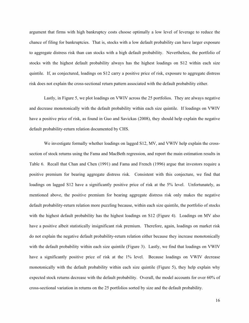
16  

argument that firms with high bankruptcy costs choose optimally a low level of leverage to reduce the

chance of filing for bankruptcies. That is, stocks with a low default probability can have larger exposure

to aggregate distress risk than can stocks with a high default probability. Nevertheless, the portfolio of

stocks with the highest default probability always has the highest loadings on S12 within each size

quintile. If, as conjectured, loadings on S12 carry a positive price of risk, exposure to aggregate distress

risk does not explain the cross-sectional return pattern associated with the default probability either.

Lastly, in Figure 5, we plot loadings on VWIV across the 25 portfolios. They are always negative

and decrease monotonically with the default probability within each size quintile. If loadings on VWIV

have a positive price of risk, as found in Guo and Savickas (2008), they should help explain the negative

default probability-return relation documented by CHS.

We investigate formally whether loadings on lagged S12, MV, and VWIV help explain the cross-

section of stock returns using the Fama and MacBeth regression, and report the main estimation results in

Table 6. Recall that Chan and Chen (1991) and Fama and French (1996) argue that investors require a

positive premium for bearing aggregate distress risk. Consistent with this conjecture, we find that

loadings on lagged S12 have a significantly positive price of risk at the 5% level. Unfortunately, as

mentioned above, the positive premium for bearing aggregate distress risk only makes the negative

default probability-return relation more puzzling because, within each size quintile, the portfolio of stocks

with the highest default probability has the highest loadings on S12 (Figure 4). Loadings on MV also

have a positive albeit statistically insignificant risk premium. Therefore, again, loadings on market risk

do not explain the negative default probability-return relation either because they increase monotonically

with the default probability within each size quintile (Figure 3). Lastly, we find that loadings on VWIV

have a significantly positive price of risk at the 1% level. Because loadings on VWIV decrease

monotonically with the default probability within each size quintile (Figure 5), they help explain why

expected stock returns decrease with the default probability. Overall, the model accounts for over 60% of

cross-sectional variation in returns on the 25 portfolios sorted by size and the default probability.

17  

Guo and Savickas (2010) show that loadings on lagged VWIV help explain the negative

idiosyncratic volatility-return relation documented by Ang, Hodrick, Xing, and Zhang (2006, 2009). To

illustrate this point, we construct the 25 value-weighted portfolios by sorting stocks first on the market

capitalization and then on idiosyncratic volatility. Loadings on lagged S12 and lagged MV increase

monotonically with the default probability within each size quintile, while loadings on lagged VWIV

decrease monotonically with the default probability.15 As reported in Table 6, we find that the price of

risk for loadings on VWIV, S12, and MV are significantly positive at the 1%, 5%, and 10% levels,

respectively. Therefore, again, only loadings on lagged VWIV help explain the negative idiosyncratic

volatility-return relation, while loadings on lagged S12 and on lagged MV suggest that the relation should

be positive, ceteris paribus. These results suggest a close link between the negative default probability-

return relation and the negative idiosyncratic volatility-return relation. This conjecture is plausible

because idiosyncratic volatility is an important determinant of the default probability.

To investigate formally the link between the default probability effect and the idiosyncratic

volatility effect, we construct the 25 value-weighted portfolios by sorting stocks first on idiosyncratic

volatility and then on the default probability. After correcting for the Fama and French 3 factors and the

momentum effect, we find that the negative default probability-return relation is statistically insignificant

except for the quintile of stocks with the highest idiosyncratic volatility. Furthermore, we construct a

hedging factor based on idiosyncratic volatility, which is the return difference between the two extreme

idiosyncratic volatility quintiles averaged across all size quintiles. We also construct a hedging factor

based on the default probability in a similar manner. The two hedging factors correlate closely with each

other, with a correlation coefficient of about 60%. Moreover, the hedging factor based on the default

probability has an insignificant alpha after we control for its loadings on (1) the hedging factor based on

                                                            15 For brevity, we do not report these results here but they are available on request.

18  

idiosyncratic volatility and (2) the momentum factor.16 To summarize, the negative default probability-

return relation reflects partly the negative idiosyncratic volatility-return relation. For brevity, we do not

report these results here but they are available on request.

As an additional robustness check, we estimate the model in equation (2) using the 25 value-

weighted portfolios sorted by the market capitalization and the Ohlson (1980) score, which we obtain

from Long Chen at Washington University. The results are qualitatively similar to those obtained using

the portfolios sorted by the default probability or idiosyncratic volatility. For example, loadings on

VWIV, which have a significantly positive price of risk, decreases with the Ohlson score within each size

quintile. Therefore, loadings on VWIV help explain the negative Ohlson (1980) score-return relation, as

documented by, e.g., Griffin and Lemmon (2002) and Chen and Zhang (2010). Moreover, as conjectured,

loadings on lagged S12 have a positive price of risk, which is statistically significant at the 10% level.

Lastly, we estimate the model in equation (2) using 75 portfolios sorted by the default probability,

idiosyncratic volatility, and the Ohlson (1980) score. Table 6 shows that loadings on VWIV, S12, and

MV have a significantly positive price of risk at the 1%, 5%, and 10% levels, respectively.

We have shown that the negative default probability-return relation documented by CHS reflects

partly the negative idiosyncratic volatility-return relation. Ang, Hodrick, Xing, and Zhang (2009) suggest

that the idiosyncratic volatility effect might reflect systematic risk because it has a strong comovement

across international stock markets. Guo and Savickas (2010) substantiate the risk-based explanation by

pointing out that stocks with high idiosyncratic volatility are usually young small firms with abundant

growth options; consequently, they are very sensitive to discount-rate shocks because their cash flows

concentrate in the distant future and thus have long durations. Therefore, stocks with high idiosyncratic

volatility tend to have low expected returns possibly because of their relatively low cash-flow betas.17 On

                                                            16 CHS (2008) find a close relation between the momentum effect and the default effect because the past losers are likely to have a higher default probability than are past winners. However, as we confirm in this paper, CHS show that the momentum factor does not fully account for the negative default probability-return relation. 17 Campbell and Vuolteenaho (2004) argue that discount-rate shocks are not as risky as cash-flow shocks because the former have only transitory effects on stock prices. Therefore, stocks with relatively high discount-rate betas,

19  

the other hand, Baker and Wurgler (2006) argue that stocks with high idiosyncratic volatility are

especially susceptible to swings in investor sentiment. Similarly, Brandt, Brav, Graham, and Kumar

(2009) suggest that there is a strong comovement between average idiosyncratic volatility and investor

sentiment. Given that invest sentiment and discount rates are two intimately related concepts—both help

explain the variation in stock prices that is unaccounted for by shocks to expected cash flows, both risk-

based and behavioral explanations suggest that stocks with high idiosyncratic volatility have a larger

portion of predictable variation than do stocks with low idiosyncratic volatility. In Figure 6, we confirm

that predictable variation increases monotonically with the default probability within each size quintile,

indicating that the negative default probability-return relation documented by CHS reflects partly

sensitivity to discount rates or investor sentiment. A formal investigation of the two alternative

explanations is clearly beyond the scope of this paper, and we leave it for future research.

To summarize, we find that stocks with a high default probability tend to have larger exposure to

aggregate distress risk than stocks with a low default probability, although the relation is not monotonic

for big stocks. Consistent with the conjecture advanced by Chan and Chen (1991) and Fama and French

(1996), we find that investors require a positive premium for bearing aggregate distress risk. These

results, however, do not explain the CHS finding of a negative default probability-return relation because

they imply that, ceteris paribus, investors require a positive, not negative, premium for holding stocks

with a high default probability. By contrast, we show that the negative default probability-return relation

reflect partly the negative idiosyncratic volatility-return relation documented by Ang, Hodrick, Xing, and

Zhang (2006, 2009). Overall, our results indicate that the default probability is a rather poor measure of

exposure to aggregate distress risk. In the next two sections, we investigate the effect of distress risk on

stock returns using the standard risk measure, i.e., the covariance with changes in aggregate distress risk.

                                                                                                                                                                                                e.g., growth stocks, tend to have lower expected returns than stocks with relatively high cash-flow betas, e.g., value stocks. Similarly, Lettau and Wachter (2007) use this intuition to show that stocks with long durations, e.g., growth stocks, tend to have lower expected returns than do stocks with short durations, e.g., value stocks.

20  

5. Forming Portfolios on Covariance with Changes in Aggregate Distress Risk

As mentioned in the introduction, several recent studies, e.g., Garlappi, Shu, and Yan (2008) and

Chava and Purnanandam (2009), show that the negative default probability-return relation reflects mainly

influence of economic forces other than aggregate distress risk. Consistent with this view, in the

preceding section, we find that loadings on lagged S12 do not explain this perverse relation. Moreover,

George and Hwang (2009) emphasize that stocks with a low default probability may have larger exposure

to aggregate distress risk than do stocks with a high default probability. These results highlight the

inappropriateness of the default probability as a measure of exposure to distress risk, as commonly used

in earlier studies. To address this issue, in this section, we reinvestigate the effect of aggregate distress

risk on the cross-section of stock returns by forming portfolios on the covariance with changes in S12,

,D iβ —a direct measure of exposure to distress risk:

(3) , , , ,12i t i M i t D i t i ter a ERET Sβ β ε= + + + .

As mentioned above, a low value of ,D iβ indicates that the stock provides a poor hedge for aggregate

distress risk; therefore, investors should require a high premium for holding it, ceteris paribus. That is,

we expect a negative relation between ,D iβ and expected stock returns.

Pastor and Stambaugh (2003) and Ang, Hodrick, Xing, and Zhang (2006) use a specification

similar to that in equation (3) to estimate exposure to aggregate illiquidity risk and aggregate volatility

risk, respectively. Following Ang, Hodrick, Xing, and Zhang (2006), we control only for market risk

because controlling for other factors in constructing portfolios based on equation (3) may add a lot of

noise. In next section, we discuss alternative specifications by controlling for other commonly used risk

factors, e.g., the size and the book-to-market factors, as in Pastor and Stambaugh (2003). We estimate

equation (3) using a 36-month rolling window; and the results are qualitatively similar if we use rolling

windows of different lengths, e.g., 60 months as in Pastor and Stambaugh (2003). We rebalance the

21  

portfolios sorted by ,D iβ every month. To ensure that our results are not simply a manifestation of

microstructure issues—e.g., bid-ask bounces—associated mainly with penny stocks, we follow Jegadeesh

and Titman (2003), among many others, and include only stocks with a price of $5 or higher.

Pastor and Stambaugh (2003) point out that the estimate of ,D iβ in equation (3) is likely to have

substantial measurement errors. This is because, for example, S12 is a noisy measure of aggregate

distress risk; there are substantial sampling errors because of relatively small sample; we do not properly

control for all the risk factors; and ,D iβ is not constant within the rolling window. Measurement errors

have an attenuate effect, which bias the estimated effect of ,D iβ on expected stock returns toward zero.

To illustrate this point, we show in next section that market beta, ,M iβ , which we estimate in the same

way as distress risk beta, ,D iβ , is never significant in the Fama and MacBeth cross-sectional regression.

With this caveat in mind, in Table 7, we show that ,D iβ nevertheless provides a reasonable measure for

exposure to aggregate distress risk by reporting summary statistics of decile portfolios sorted by ,D iβ .

In panel A of Table 7, we report the median of main characteristics of stocks in each decile

portfolio for the formation period. We find that ,D iβ increases monotonically from decile 1 to decile 10.

This pattern, of course, reflects simply the fact that we form portfolios by sorting stocks on ,D iβ .

Nevertheless, ,D iβ exhibits a large cross-sectional dispersion, ranging from -1.08 for decile 1 to 0.32 for

decile 10, indicating that the effect of aggregate distress risk varies substantially across stocks. This result

is important because, as emphasized by Ang, Hodrick, Xing, and Zhang (2006), a large dispersion in the

independent variable, i.e., ,D iβ , allows us to estimate precisely its relation with expected stock returns.

Earlier authors, e.g., Dichev (1998), Griffin and Lemmon (2002), and CHS, use various default

probability measures as a proxy of exposure to aggregate distress risk. That is, they assume that stocks

22  

with a high default probability are likely to have a low ,D iβ . To investigate this hypothesis, in Figure 7,

we plot median formation period ,D iβ of decile portfolios sorted by ,D iβ (triangles) along with that of

decile portfolios sorted by the default probability (squares). For default probability-sorted portfolios,

decile 1 is the portfolio of stocks with the highest default probability and decile 10 is the portfolio of

stocks with the lowest default probability. We expect similar patterns under the assumption adopted in

earlier studies; the difference between two sorts, however, is striking. Compared with portfolios sorted by

,D iβ , loadings on changes in aggregate distress risk are rather flat across portfolios sorted by the default

probability. More importantly, ,D iβ is a hump-shaped function of the default probability, indicating that

stocks with the lowest default probability are not least vulnerable to aggregate distress risk. This result

corroborates George and Hwang’s (2009) conjecture that the endogeneity of leverage due to

heterogeneous bankruptcy costs is important for understanding the perverse negative relation between the

default probability and expected returns. Intuitively, firms with high bankruptcy costs choose optimally a

low level of leverage to reduce their default probability; of course, these firms may still be quite sensitive

to distress risk because of their high bankruptcy costs. In particular, in their Proposition 1, George and

Hwang (2009) argue that leverage is an inverse measure of exposure to distress risk. Consistent with this

hypothesis, in Table 7, we show that leverage constructed using the book values of long-term debts and

assets, LEV, decreases monotonically with exposure to aggregate distress risk except for decile 10.18 To

summarize, the default probability is a rather poor measure of exposure to aggregate distress risk.

As shown in Table 7, we find that the median default probability over the 12-month horizon, P12,

decreases from decile 1 to decile 10; however, the cross-sectional variation is rather moderate. To

illustrate clearly this point, in Figure 8, we plot the median default probability for decile portfolios sorted

by ,D iβ (triangles) along with that for decile portfolios sorted by the default probability (squares). The

                                                            18 If sorting stocks into deciles by the default probability, we find that leverage increases monotonically from the decile of stocks with the least default probability to the decile of stocks with the highest default probability. This result, according to Proposition 1 in George and Hwang (2009), casts doubt that the default probability is a measure of exposure to aggregate distress risk.

23  

difference between two sorts is again striking. While the median default probability decreases sharply

from decile 1 to decile 10 for the default probability-sorted portfolios, the pattern is rather flat across the

,D iβ -sorted portfolios. The relatively weak relation between ,D iβ and the default probability in ,D iβ -

sorted portfolios has important implications for identification in the empirical analysis—it allows us to

distinguish the effect of ,D iβ (as a systematic risk) from the effect of the default probability (as a

characteristic) on expected stock returns in the cross-sectional regression. In particular, Garlappi, Shu,

and Yan (2008) show that stocks with a high default probability have abnormally low future returns

because equity investors have anticipated claims on a substantial portion of a firm’ assets when the firm

eventually files for bankruptcy. Chava and Purnanandam (2009) suggest that realized future returns are a

rather poor proxy of expected returns for portfolios of stocks with a high default probability because their

realized returns tie tightly to actual bankruptcy outcomes. In particular, Chava and Purnanandam show

that the negative cross-sectional relation between the default probability and future returns reflects mainly

the fact that the actual number of bankruptcies in the post-1980 sample is substantially high than what

investors had expected ex ante. Both studies suggest that the negative default probability-return relation

reflects influence of economic forces other than aggregate distress risk. Because of a weak relation

between ,D iβ and the default probability (Figure 8), these economic forces should have a substantially

smaller, if any, effect on the relation between ,D iβ and expected stock returns.

Table 7 reveals a negative relation between median ,D iβ and median idiosyncratic volatility,

which decreases from 3.0% for decile 1 to 1.8% for decile 10. This result should not be too surprising

because stocks with high idiosyncratic volatility are likely to have a higher default probability (see, e.g.,

CHS) and thus are more vulnerable to aggregate distress risk than stocks with low idiosyncratic volatility,

ceteris paribus. Ang, Hodrick, Xing, and Zhang (2006, 2009) document a robust negative cross-sectional

relation between idiosyncratic volatility and future stock returns in both U.S. and international stock

markets, although there is an ongoing debate about economic explanations of such a relation. Under our

24  

maintained hypothesis, we expect a negative relation between ,D iβ and expected stock returns. Because

stocks with a low ,D iβ tend to have high idiosyncratic volatility, their expected returns, however, could be

either high or low, depending on the relative strengthen of the distress effect and the idiosyncratic

volatility effect. To summarize, the close relation between ,D iβ and idiosyncratic volatility highlights the

importance that we should control for idiosyncratic volatility when investigating the cross-sectional

relation between ,D iβ and expected stock returns to alleviate the omitted variables problem.

As shown in Table 7, the median market capitalization (SIZE) increases monotonically from

decile 1 to decile 10. This pattern is consistent with Chan and Chen’s (1991) conjecture that small firms

are especially vulnerable to financial distress. The median book-to-market equity ratio (BM), however, is

a hump-shaped function of median ,D iβ —it increases from 0.50 for decile 1 to 0.65 for decile 5 and then

decreases to 0.52 for decile 10. This pattern appears to suggest that, by contrast with Fama and French’s

(1992) conjecture, BM is a rather poor measure of exposure to aggregate distress risk. The median

return-on-equity increases almost monotonically from decile 1 to decile 10, indicating that profitable

firms are less vulnerable to aggregate distress risk than are stocks that recently suffer from substantial

operating losses. This result should not be too surprising—profitable firms can use retained earnings as a

buffer for distress risk. Nevertheless, it confirms that ,D iβ provides a reasonable measure of exposure to

aggregate distress risk. Lastly, there is no obvious correlation of the short-term return reversal (RET_1)

or momentum (RET_72) with exposure to aggregate distress risk.

In panel B of Table 7, we report the sample average of equal-weighted portfolio returns on decile

portfolios sorted by ,D iβ . Consistent with our maintained hypothesis, the portfolio of stocks that are most

vulnerable to aggregate distress risk (decile 1) has a higher average return than does the portfolio of

stocks that are least vulnerable to aggregate distress risk (decile 10). Panel C shows that results are

qualitatively similar for value-weighted portfolio returns. These results are in sharp contrast with those

25  

reported in CHS (2008, 2010), who use the default probability as a measure of exposure to distress risk

and find a strong negative relation between distress risk and expected stock returns. The difference

corroborates the recent findings, e.g., Garlappi, Shu, and Yan (2008), Chava and Purnanandam (2009),

and George and Hwang (2009), that the default probability is a rather poor measure of distress risk.

While our results cast doubt on earlier evidence that investors require a negative premium for

bearing aggregate distress risk, they provide little support for the conjecture of a positive distress risk

premium either. In particular, although the return difference between deciles 1 and 10 is positive, it is

economically small and statistically insignificant at the conventional level. Moreover, panels B and C of

Table 7 show that expected returns are a hump-shaped function of ,D iβ . One possible explanation is that

while loadings on changes in aggregate distress risk are potentially an important determinant of the cross-

section of expected returns, they are not the only determinant. In particular, as we mentioned above, a

stock with low ,D iβ tends to have high idiosyncratic volatility. Because ,D iβ and idiosyncratic volatility

both have negative effects on expected stock returns, the insignificant relation between ,D iβ and expected

stock returns may reflect the omitted variables problem. We illustrate this point below by explicitly

controlling for idiosyncratic volatility when forming portfolios by ,D iβ ; in next section, we address

formally the omitted variables problem using the Fama and MacBeth cross-sectional regression.

To address the omitted variables problem due to the close relation between ,D iβ and idiosyncratic

volatility, we first sort stocks equally into five quintiles by idiosyncratic volatility. For each idiosyncratic

volatility quintile, we then sort stocks equally into five quintiles by ,D iβ . In Table 8, for each

idiosyncratic volatility quintile, we report the return difference between the low and high ,D iβ quintiles.

Panel A is the results for equal-weighted portfolio returns. As conjectured, after controlling for

idiosyncratic volatility, we find that the return difference between low and high ,D iβ stocks is positive

and statistically significant at least at the 5% level for three bottom idiosyncratic volatility quintiles. The

26  

return difference remains significant after controlling for market risk, while Fama and French three

factors account for a substantial portion of the distress risk premium. The latter result is consistent with

the conjecture advanced by Chan and Chen (1991) and Fama and French (1996) that the size and B/M

effects reflect mainly aggregate distress risk. Nevertheless, for the quintile of stocks with the smallest

idiosyncratic volatility, the return difference remains statistically significant at the 10% level after

controlling for the Fama and French three factors, indicating that the size and B/M effects do not fully

account for the distress risk. We find qualitatively similar results using the Fama and French 3-factor

model augmented by a momentum factor. The distress premium is positive for quintile 4 and is negative

for quintile 5, although statistically insignificant for both quintiles. The difference in distress effects

between low and high idiosyncratic volatility quintiles provides an interesting example for the argument

that idiosyncratic risk is the single largest impediment to arbitrage (see, e.g., Ali, Hwang, Trombley

(2003) and Pontiff (2006)). With this caveat in mind, the results in panel A of Table 8 provide strong

support for the hypothesis that investors require a positive premium for bearing aggregate distress risk.

In panel B of Table 8, we show that the results obtained from value-weighted portfolio returns are

qualitatively similar to, but somewhat weaker than, their equal-weighted counterpart, as reported in panel

A of Table 8. For example, the return difference between low and high ,D iβ stocks is positive and

significant for the three bottom idiosyncratic volatility quintiles. The return difference, however,

becomes negligible after we control for the Fama and French three factors, even for the quintile of stocks

with the lowest idiosyncratic volatility. The relatively weak distress effect for value-weighted portfolios

is consistent with Chan and Chen’s (1991) conjecture that small firms are more susceptible to distress risk

than are big firms (see also Vassalou and Xing (2004)).

We also investigate the relation between ,D iβ and expected stock returns by explicitly controlling

for the default probability. As mentioned in Section 3, there is a close link between the negative default

probability-return relation and the negative idiosyncratic volatility-return relation because idiosyncratic

27  

volatility is an important determinant of the default probability. Therefore, similar to controlling for

idiosyncratic volatility, controlling for the default probability may help uncover a positive distress risk

premium as well. This exercise also illustrates the difference between ,D iβ and the default probability.

In panel A of Table 9, we report the distress risk premium for equal-weighted portfolio returns.

As expected, for the quintile of stocks with the lowest default probability, the distress risk premium is

economically large and statistically significant at the 1% level, with and without the control for its

loadings on commonly used risk factors. The distress premium, however, is significantly negative for the

quintile of stocks with the highest default probability. There are three possible explanations for the

perverse negative distress risk premium documented in the high default probability quintile. First, CHS

show that stocks with a high default probability are vulnerable to mispricing because they usually have

large arbitrage costs. Second, these stocks are more susceptible to investment sentiment because of large

uncertainty about their fundamentals (Baker and Wurgler (2006)). Lastly, because returns on these

stocks tie closely to the actual outcome of bankruptcies, the negative distress risk premium reflect partly

the fact that the actual default rate is higher than what investors had anticipated (Chava and Purnanandam

(2009)). By contrast, the market imperfection is likely to have smaller effects on stocks with a low

default probability, for which we find a significantly positive distress risk premium. In panel B of Table

9, we find qualitatively similar results for value-weighted portfolio returns. Overall, the double-sort by

the default probability and ,D iβ provides additional support for a positive distress risk premium.

Lastly, we investigate the effect of ,D iβ on expected stock returns by explicitly controlling for the

market capitalization. Again, we construct the 25 portfolios by first sorting stocks on the market

capitalization and then sorting stocks on ,D iβ . For the quintile of stocks with the biggest market

capitalization, expected returns decrease monotonically with ,D iβ , although the return difference between

the lowest and highest ,D iβ quintiles is statistically insignificant. For brevity, we do not report these

28  

results here but they are available on request. We also estimate the model in equation (2) using the 25

portfolios sorted by size and ,D iβ , and report the Fama and MacBeth regression results in Table 6. Again,

we find that loadings on lagged S12 have a positive price of risk, although it is statistically insignificant.

We also estimate the model in equation (2) using 100 portfolios, including the 25 portfolios sorted by size

and the default probability, the 25 portfolios sorted by size and idiosyncratic volatility, the 25 portfolios

sorted by size and the Ohlson (1980) score, and the 25 portfolios sorted by size and ,D iβ . With a large

number of portfolios, we estimate the effect of aggregate distress risk on expected stock returns precisely.

In particular, consistent with our maintained hypothesis, loadings on lagged S12 have a significantly

positive price of risk at the 5% level.

6. Stock-Level Fama and MacBeth Regressions

In the preceding section, we show that investors require a positive premium for bearing aggregate

distress risk when controlling for the effect of idiosyncratic volatility on expected returns. We illustrate

this point by sorting stocks first on idiosyncratic volatility and then on ,D iβ . In this section, we address

the issue formally using the stock-level Fama and MacBeth cross-sectional regression. An appealing

advantage of the Fama and MacBeth regression is that it allows us to simultaneously control for various

measures of risk or characteristics that forecast the cross-section of stock returns.

In row 1 of Table 10, we use market beta, ,M iβ , and distress beta, ,D iβ , to explain the cross-

section of stock returns. Consistent with the maintained hypothesis that investors require a positive

premium for bearing aggregate distress risk, there is a negative relation between ,D iβ and expected

returns; the relation, however, is statistically insignificant at the conventional level. Consistent with the

evidence reported in Section 6, the negative effect of ,D iβ on expected stock returns becomes statistically

significant at the 5% level if we control for idiosyncratic volatility in the cross-sectional regression (row

29  

2). As in Ang, Hodrick, Xing, and Zhang (2006, 2009), we also find that idiosyncratic volatility has a

significantly negative effect on expected returns. The absolute value of the risk premium on ,D iβ almost

doubles with the control of idiosyncratic volatility (row 2) relative to that without the control (row 1).

These results suggest that the insignificant relation between ,D iβ and expected stock returns documented

in row 1 reflects the omitted variables problem— ,D iβ correlates negatively with idiosyncratic volatility,

while both variables correlate negatively with expected stock returns.

Similarly, row 3 of Table 10 shows that the negative effect of ,D iβ becomes marginally

significant when we control for the default probability, S12, which have a significantly negative effect on

expected returns, as documented in CHS (2008, 2010). The effect of ,D iβ remains significantly negative

at the 5% level after we control for both idiosyncratic volatility and the default score (row 4). These

results again confirm that the negative default probability-return relation documented by CHS does not

reflect the effect of aggregate distress risk on expected returns; otherwise, we would expect that the effect

of ,D iβ on expected returns should become less, not more, significant when controlling for S12 in the

cross-sectional regression due to the multicollinearity problem.

Table 10 shows that the effect of ,D iβ on expected stock returns remains significantly negative

when we add other commonly used predictors of cross-sectional stock returns in the Fama-MacBeth

regression, including the momentum (RET_7-2), the short-term return reversal (RET_1), and leverage

(LEV), either individually or jointly. We find a similar result by controlling for the book-to-market ratio

(BM). By contrast, the effect of ,D iβ becomes statistically insignificant when we control for the market

capitalization (SIZE). The latter result is consistent with the Chan and Chen’s (1991) conjecture that the

size effect reflects mainly distress risk.

30  

To investigate further the relation between the distress risk and the size effect, we add the size

(SMB) and the book-to-market (HML) factors as additional control when estimating loadings on changes

in aggregate distress risk:

(4) , , , , , ,12i t i M i t D i t SMB i t HML i t i ter a ERET S SMB HMLβ β β β ε= + + + + + .

In this case, we find an insignificant relation between ,D iβ and expected stock returns, even when

controlling for idiosyncratic volatility and the default probability in the cross-sectional regression. These

results, again, suggest a close relation between the size effect and the distress risk. For brevity, we do not

report them here but they are available on request.

We also investigate whether the distress risk effect relates to the illiquidity risk effect, as

documented by Pastor and Stambaugh (2003) and Acharya and Pedersen (2005), among others. Pastor

and Stambaugh propose a novel measure of aggregate liquidity, PSLIQ, and find that loadings on

unexpected changes in PSLIQ have significant predictive power for the cross-section of stock returns. To

investigate the link between the distress risk and the illiquidity risk, we estimate loadings on changes in

aggregate distress risk by explicitly controlling for changes in PSLIQ:

(5) , , , , ,12i t i M i t D i t PSLIQ i t i ter a ERET S PSLIQβ β β ε= + + + + .

We find that controlling for liquidity risk has negligible effects on the relation between ,D iβ and expected

stock returns documented in Table 10. This result is consistent with that reported in Table 4, in which we

show that controlling for PSLIQ does not affect the predictive power of S12 for excess market returns.

Consistent with evidence in Amihud (2002), Acharya and Pedersen (2005) find that illiquid socks tend to

have higher expected returns than do liquid stocks. We find that controlling for Amihud’s (2002)

illiquidity measure in the cross-sectional regression has negligible effects on the results reported in Table

10. For brevity, we do not report these results here but they are available on request.

31  

7. Conclusion

Earlier authors, e.g., Chan and Chen (1991) and Fama and French (1996), have conjectured that

stocks with a small market capitalization or a high book-to-market equity ratio earn abnormally high

CAPM-adjusted returns because they provide a poor hedge for aggregate distress risk and investors

require a positive premium for holding them. Using a stock’s default probability as a proxy of the stock’s

exposure to aggregate distress risk, Dichev (1998), Griffin and Lemmon (2002), and CHS (2008, 2010),

however, find a perverse negative distress risk premium.

In this paper, we note that the default probability is a rather poor measure of loadings on

aggregate distress risk. In particular, consistent with recent findings in Garlappi, Shu, and Yan (2008),

Chava and Purnanandam (2009), and George and Hwang (2009), we show that the negative default

probability-return reflects influence of economic forces other than aggregate distress risk. We then revisit

the pricing of systematic distress risk in the stock market in three ways. First, aggregate default

probability forecasts excess market returns when in conjunction with other determinants of conditional

equity premium. Second, loadings on lagged systematic default probability are significantly priced in the

cross-section of stocks returns with a positive premium. Lastly, when we use the standard risk measure—

i.e., the covariance with changes in aggregate default probability, instead of the default probability, as a

proxy of exposure to distress risk, we uncover a positive and significant distress premium. We also

document a close relation between the distress risk and the size effect, as conjectured by Chan and Chen

(1991). The relation between distress risk and the book-to-market effect, as conjectured by Fama and

French (1996), however, is relatively weak in the data.

We also document a strong interaction between idiosyncratic volatility and distress risk.

Aggregate default probability forecasts excess market returns only when we control for the effect of

average idiosyncratic variance on conditional equity premium, as documented by Guo and Savickas

(2008). Similarly, the covariance with changes in aggregate default probability has significant

32  

explanatory power for the cross-section of stocks returns only when we control for the effect of

idiosyncratic volatility on expected stock returns, as documented in Ang, Hodrick, Xing, and Zhang

(2006, 2009). It is beyond the scope of this paper to explore the nature of such an interaction, and we

leave it for future research.

33  

References

Acharya, V., and L. Pedersen, 2005, Asset Pricing with Liquidity Risk, Journal of Financial Economics,

77, 375–410.

Ali, A., L. Hwang, and M. Trombley, 2003, Arbitrage Risk and the Book-to-Market Anomaly, Journal of

Financial Economics, 69, 355-373.

Amihud, Y., 2002, Illiquidity and Stock Returns, Journal of Financial Markets, 5, 31-56.

Andersen, T., T. Bollerslev, F. Diebold, and P. Labys, 2003, Modeling and Forecasting Realized

Volatility, Econometrica, 71, 579-625.

Ang, A., R. Hodrick, Y. Xing, and X. Zhang, 2006, the Cross-Section of Volatility and Expected Returns,

Journal of Finance, 51, 259-299.

Ang, A., R. Hodrick, Y. Xing, and X. Zhang, 2009, High Idiosyncratic Volatility and Low Returns:

International and Further U.S. Evidence, Journal of Financial Economics, 91, 1-23.

Baker, M., and J. Wurgler, 2006, Investor Sentiment and the Cross-Section of Stock Returns, Journal of

Finance, 61, 1645-1680.

Bharath, S., and T. Shumway, 2008, Forecasting Default with the Merton Distance to Default Model,

Review of Financial Studies, 21, 1339–1369.

Bernanke, S., and M. Gertler, 1989, Agency Costs, Net Worth, and Business Fluctuations, American

Economic Review, 79, 14-31.

Black, F., and M. Scholes, 1973, The Pricing of Options and Corporate Liabilities, Journal of Political

Economy, 81, 637-659.

34  

Brandt, M., A. Brav, J. Graham, and A. Kumar, 2009, The Idiosyncratic Volatility Puzzle: Time Trend or

Speculative Episodes?, Review of Financial Studies, forthcoming.

Brunnermeier, M., and L. Pedersen, 2009, Market Liquidity and Funding Liquidity, Review of Financial

Studies, 22, 2201-2199.

Campbell, J., 1993, Intertemporal Asset Pricing Without Consumption Data, American Economic

Review, 83, 487-512.

Campbell, J. and J. Cochrane, 1999, By Force of Habit: A Consumption-Based Explanation of Aggregate

Stock Market Behavior, Journal of Political Economy, 107, 205-251.

Campbell, J., J. Hilscher, and J. Szilagyi, 2008, In Search of Distress Risk, Journal of Finance, 63, 2899-

2939.

Campbell, J., J. Hilscher, and J. Szilagyi, 2010, Predicting Financial Distress and the Performance of

Distressed Stocks, Journal of Investment Management, forthcoming.

Campbell, J., M. Lettau, B. Malkiel, and Y. Xu, 2001, Have Individual Stocks Become More Volatile?

An Empirical Exploration of Idiosyncratic Risk, Journal of Finance, 56, 1-43.

Campbell, J., T. Vuolteenaho, 2004, Bad Beta, Good Beta, American Economic Review, 94, 1249-1275.

Chan, K., and N. Chen, 1991, Structural and Return Characteristics of Small and Large Firms, Journal of

Finance, 46, 1467–1484.

Chava, S., and R. Jarrow, 2004, Bankruptcy Prediction with Industry Effects, Review of Finance 8, 537–

569.

Chava, S., and A. Purnanandam, 2009, Is Default Risk Negatively Related to Stock Returns? Review of

Financial Studies, forthcoming.

35  

Chen, L., P. Collin-Dufresne, and R. Goldstein, 2009, On the Relation Between the Credit Spread Puzzle

and the Equity Premium Puzzle, Review of Financial Studies, forthcoming.

Chen, L., D. Lesmond, and J. Wei, 2007, Bond Liquidity Estimation and the Liquidity Effect in Yield

Spreads, Journal of Finance, 62, 119–149.

Chen, L., and L. Zhang, 2010, A Better Three-Factor Model that Explains More Anomalies, Journal of

Finance, forthcoming.

Collin-Dufresne, P., R. Goldstein, and J. Martin, 2001, The Determinants of Credit Spread Changes,

Journal of Finance, 56, 2177–2207.

Cochrane, J., 1991, Production-Based Asset Pricing and the Link between Stock Returns and Economic

Fluctuations, Journal of Finance, 46, 209–237.

Da, Z., and P. Gao, 2008, Clientele Change, Liquidity shock, and the Return on Financially Distressed

Stocks, Journal of Financial and Quantitative Analysis, forthcoming.

Dichev, I., 1998, Is the Risk of Bankruptcy a Systematic Risk? Journal of Finance, 53, 1141–1148.

Elliott, G., T. Rothenberg,, and J. Stock, 1996, Efficient Tests for an Autoregressive Unit Root,

Econometrica, 64, 813–836.

Elton, E., M. Gruber, D. Agrawal, and C. Mann, 2001, Explaining the Rate Spread on Corporate Bonds,

Journal of Finance, 56, 247–277.

Fama, E. and K. French, 1989, Business Conditions and Expected Returns on Stocks and Bonds, Journal

of Financial Economics, 25, 23-49.

Fama, E., and K. French, 1996, Multifactor Explanations of Asset Pricing Anomalies, Journal of Finance,

51, 55–84.

36  

Fama, E., and J. MacBeth, 1973, Risk, Return, and Equilibrium: Empirical Tests, Journal of Political

Economy, 71, 607–636.

Ferguson, M., and R. Shockley, 2003, Equilibrium “Anomalies,” Journal of Finance, 58, 2549–2580.

French, K., W. Schwert, and R. Stambaugh, 1987, Expected Stock Returns and vVlatility, Journal of

Financial Economics, 19, 3-30.

Garlappi, L., T. Shu, and H. Yan, 2008, Default Risk, Shareholder Advantage, and Stock Returns, Review

of Financial Studies, 21, 2743-2778.

George, T., and C. Hwang, 2009, A Resolution of the Distress Risk and Leverage Puzzles in the Cross

Section of Stock Returns, Journal of Financial Economics, forthcoming.

Gertler, M., and N. Kiyotaki, 2009, Financial Intermediation and Credit Policy in Business Cycle

Analysis, Unpublished working paper, NYU and Princeton.

Ghysels, E., P. Santa-Clara, and R. Valkanov, 2005, There is a Risk-Return Tradeoff after all, Journal of

Financial Economics, 76, 509-548.

Goyal, A., and I. Welch, 2008, A Comprehensive Look at the Empirical Performance of Equity Premium

Prediction, Review of Financial Studies, 21, 1455-1508.

Griffin, J., and M. Lemmon, 2002, Book-to-Market Equity, Distress Risk, and Stock Returns, Journal of

Finance, 57, 2317–2336.

Guo, H., and R. Whitelaw, 2006, Uncovering the Risk-Return Relation in the Stock Market, Journal of

Finance, 61, 1433-1463.

Guo, H., and R. Savickas, 2008, Average Idiosyncratic Volatility in G7 Countries, Review of Financial

Studies, 21, 1259-1296.

37  

Guo, H., and R. Savickas, 2010, Relation between Time-Series and Cross-Sectional Effects of

Idiosyncratic Variance on Stock Returns, Journal of Banking and Finance, forthcoming.

Huang, J., and M. Huang, 2003, How Much of the Corporate-Treasury Yield Spread is due to Credit

Risk? A New Calibration Approach, Unpublished working paper, Stanford University.

Jagannathan, R., and Z. Wang, The Conditional CAPM and the Cross-Section of Expected Returns,

Journal of Finance, 51, 3-53.

Keim, D., and R. Stambaugh, 1986, Predicting Returns in the Stock and Bond Markets, Journal of

Financial Economics, 17, 357-390.

Kiyotaki, N., and J. Moore, 1997, Credit Cycles, Journal of Political Economy, 105, 211-248.

Lettau, M., and S. Ludvigson, 2005, tay's As Good as cay: Reply, Finance Research Letters, 2, 15-22.

Lettau, M., and J. Wachter, 2007, Why is Long-Horizon Equity Less Risky? A Duration-Based

Explanation of the Value Premium, Journal of Finance, 62, 55-92.

Lustig, H., and S. Van Nieuwerburgh, 2005, Housing Collateral, Consumption Insurance and Risk

Premia: an Empirical Perspective, Journal of Finance, 60, 1167-1219.

Merton, R., 1973, An Intertemporal Capital Asset Pricing Model, Econometrica, 41, 867-887.

Merton, R., 1974, On the Pricing of Corporate Debt: The Risk Structure of Interest Rates, Journal of

Finance, 29, 449-470.

Merton, R., 1980, On Estimating the Expected Return on the Market: An Exploratory Investigation,

Journal of Financial Economics, 8, 323-61.

Ohlson, J., 1980, Financial Ratios and the Probabilistic Prediction of Bankruptcy, Journal of Accounting

Research, 19, 109-131.

38  

Pastor, L., and R. Stambaugh, 2003, Liquidity risk and expected stock returns, Journal of Political

Economy, 111, 642–685.

Piazzesi, M., M. Schneider, and S. Tuzel, 2007, Housing, Consumption and Asset Pricing, Journal of

Financial Economics 83, 531-569.

Pontiff, J., 2006, Costly Arbitrage and the Myth of Idiosyncratic Risk, Journal and Accounting and

Economics, 42, 35-52.

Scruggs, J., 1998, Resolving the Puzzling Intertemporal Relation Between the Market Risk Premium and

Conditional Market Variance: A Two-Factor Approach, Journal of Finance, 53, 575-603.

Shumway, T., 2001, Forecasting Bankruptcy More Accurately: A Simple Hazard Model, Journal of

Business 74, 101–124.

Vassalou, M., and Y. Xing, 2004, Default Risk in Equity Returns, Journal of Finance 59, 831–868.

39  

Figure 1: Aggregate Default Score over 12-Month Horizon (S12)

Figure 2: Aggregate Default Probability over 12-Month Horizon (P12)

‐0.08

‐0.07

‐0.06

Dec‐71 Nov‐76 Nov‐81 Nov‐86 Nov‐91 Nov‐96 Nov‐01 Nov‐06

0.00

0.10

0.20

0.30

0.40

0.50

Dec‐71 Nov‐76 Nov‐81 Nov‐86 Nov‐91 Nov‐96 Nov‐01 Nov‐06

40  

Figure 3: Loadings on MV for 25 Portfolios Sorted by Size and Default Probability

Figure 4: Loadings on S12 for 25 Portfolios Sorted by Size and Default Probability

0.00

5.00

10.00

15.00

20.00

25.00

S1D1

S1D2

S1D3

S1D4

S1D5

S2D1

S2D2

S2D3

S2D4

S2D5

S3D1

S3D2

S3D3

S3D4

S3D5

S4D1

S4D2

S4D3

S4D4

S4D5

S5D1

S5D2

S5D3

S5D4

S5D5

0

5

10

15

20

25

30

S1D1

S1D2

S1D3

S1D4

S1D5

S2D1

S2D2

S2D3

S2D4

S2D5

S3D1

S3D2

S3D3

S3D4

S3D5

S4D1

S4D2

S4D3

S4D4

S4D5

S5D1

S5D2

S5D3

S5D4

S5D5

41  

Figure 5: Loadings on VWIV for 25 Portfolios Sorted by Size and Default Probability

Figure 6: R2 for 25 Portfolios Sorted by Size and Default Probability

‐8.00

‐7.00

‐6.00

‐5.00

‐4.00

‐3.00

‐2.00

‐1.00

0.00

S1D1

S1D2

S1D3

S1D4

S1D5

S2D1

S2D2

S2D3

S2D4

S2D5

S3D1

S3D2

S3D3

S3D4

S3D5

S4D1

S4D2

S4D3

S4D4

S4D5

S5D1

S5D2

S5D3

S5D4

S5D5

0

0.05

0.1

0.15

0.2

0.25

0.3

S1D1

S1D2

S1D3

S1D4

S1D5

S2D1

S2D2

S2D3

S2D4

S2D5

S3D1

S3D2

S3D3

S3D4

S3D5

S4D1

S4D2

S4D3

S4D4

S4D5

S5D1

S5D2

S5D3

S5D4

S5D5

42  

Figure 7: Median Stock Loadings on S12Δ for Deciles Portfolios Sorted by Loadings on S12Δ (Triangles) and for Deciles Sorted by Default Probability (Squares)

Figure 8: Median Default Probability for Deciles Portfolios Sorted by Loadings on S12Δ (Triangles) and for Deciles Portfolios Sorted by Default Probability (Squares)

‐1.2

‐1.0

‐0.8

‐0.6

‐0.4

‐0.2

0.0

0.2

0.4

1 2 3 4 5 6 7 8 9 10

0.0

0.1

0.2

1 2 3 4 5 6 7 8 9 10

43  

Table 1 Summary Statistics

Panel A Univariate Statistics ERET MV VWIV S12 P12 ΔS12 ΔP12 Mean 0.011 0.007 0.021 -0.073 0.137 0.000 0.002 SD 0.089 0.010 0.017 0.003 0.065 0.002 0.035 Autocorrelation 0.054 0.333 0.809 0.812 0.804 -0.214 -0.088 Unit Root Test -11.078*** -2.814*** -2.469** -3.279** -3.064** -11.932*** -1.552

Panel B Cross-Correlations ERET 1.000 -0.401 -0.293 -0.193 -0.197 -0.457 -0.444 MV 1.000 0.645 0.527 0.487 0.487 0.555 VWIV 1.000 0.609 0.568 0.282 0.371 S12 1.000 0.920 0.355 0.356 P12 1.000 0.306 0.358 ΔS12 1.000 0.875 ΔP12 1.000

Note: We report summary statistics for selected variables used in the paper. The sample spans the 1972Q1 to 2008Q4 period. ERET is excess market return; MV is realized market variance; VWIV is value-weighted average idiosyncratic variance; S12 is average default score over the 12-month horizon; P12 is average default probability over the 12-month horizon; ΔS12 is the first difference of S12; and ΔP12 is the first difference of P12. We construct the default score or probability using parameter estimates of the logit model reported in CHS (2010). We use Elliott, Rothenberg, and Stock (1996) unit root test, and allow for a linear time trend for S12 and P12. We also use detrended S12 and P12 when calculating the autocorrelation and cross-correlation. ***, **, and * denote significance at the 1%, 5%, and 10% levels, respectively.

44  

Table 2 Forecasting Excess Market Returns Using Aggregate Default Risk

S12 MV VWIV P12 V_HML Adjusted R2

Panel A Quarterly Data 1971Q4 to 2008Q4 1 2.861

(2.726) -0.006

2 6.559*** (1.489)

-2.712*** (0.513)

0.098

3 5.095*** (1.348)

-16.833*** (2.735)

0.096

4 6.257*** (1.444)

-1.608* (0.838)

-8.154 (6.149)

0.100

5 10.448*** (2.744)

-2.214*** (0.474)

0.079

6 8.540*** (2.341)

-14.642*** (2.583)

0.082

7 9.838*** (2.673)

-1.068 (0.876)

-8.555 (6.297)

0.081

8 2.045 (2.659)

0.674 (1.622)

-0.012

9 7.378*** (2.539)

5.275*** (1.301)

-3.181*** (0.569)

0.122

10 5.287** (2.295)

3.842*** (1.262)

-18.252*** (2.699)

0.105

11 7.035*** (2.502)

5.105*** (1.278)

-2.320*** (0.928)

-6.198 (6.067)

0.120

12 -1.923*** (0.527)

0.417*** (0.133)

0.063

13 5.747*** (1.424)

-3.117*** (0.636)

0.308** (0.126)

0.114

Panel B Annual Data 1972 to 2009

14 10.613 (7.969)

-0.018

15 6.362*** (0.771)

-4.658*** (0.955)

0.084

16 27.913*** (6.726)

-4.133** (1.743)

0.046

17 22.933*** (6.988)

5.539*** (0.759)

-6.950*** (1.550)

0.141

18 -4.595** (1.930)

1.415*** (0.454)

0.082

19 5.520*** (0.824)

-7.487*** (1.542)

1.224*** (0.404)

0.178

Note: We report the OLS estimation results of forecasting excess market returns. S12 is average default score over the 12-month horizon; MV is realized market variance; VWIV is value-weighted average idiosyncratic variance; P12 is average default probability over the 12-month horizon; and V_HML is realized variance of the value premium. We construct the default score or probability using the parameter estimates of the logit model reported in CHS (2010). We report Newey-West standard errors in parentheses with four lags for quarterly data and one lag for annual data. ***, **, and * denote significance at the 1%, 5%, and 10% levels, respectively.

45  

Table 3 Forecasting Excess Market Returns Using Alternative Measures of Aggregate Distress Risk: 1971Q4 to 2008Q4

S1 S36 P1 P36 MV VWIV Adjusted R2

Panel A Parameter Estimates in CHS (2010) 1 3.412**

(1.568) 5.241***

(1.357) -2.870***

(0.547) 0.112

2 8.702*** (3.135)

5.886*** (1.372)

-3.308*** (0.579)

0.122

3 0.184 (0.114)

5.957*** (1.463)

-2.809*** (0.576)

0.106

4 0.631*** (0.215)

6.091*** (1.450)

-3.470*** (0.615)

0.128

Panel B Default Score Based on Parameter Estimates in CHS (2008) S1 S6 S12 S24 S36 MV VWIV Adjusted R2

5 3.448** (1.602)

5.306*** (1.351)

-2.862*** (0.544)

0.112

6 5.474** (2.169)

5.252*** (1.323)

-2.959*** (0.553)

0.117

7 6.986*** (2.481)

5.414*** (1.314)

-3.135*** (0.563)

0.121

8 7.972*** (2.776)

5.699*** (1.343)

-3.276*** (0.570)

0.123

9 7.957** (3.250)

6.060*** (1.393)

-3.255*** (0.580)

0.118

Panel C Default Probability Based on Parameter Estimates in CHS (2008) P1 P6 P12 P24 P36 MV VWIV Adjusted R2

10 0.201 (0.128)

5.995*** (1.468)

-2.804*** (0.572)

0.105

11 0.230* (0.118)

5.843*** (1.441)

-2.890*** (0.596)

0.111

12 0.333** (0.141)

5.825*** (1.436)

-3.084*** (0.627)

0.117

13 0.495*** (0.171)

5.946*** (1.443)

-3.403*** (0.629)

0.126

14 0.598*** (0.216)

6.255*** (1.463)

-3.475*** (0.612)

0.126

46  

Note: We report the OLS estimation results of forecasting one-quarter-ahead excess market returns using alternative measures of aggregate distress risk. S1, S6, S12, S24, and S36 are average default scores over the 1-, 6-, 12-, 24, and 36-month horizons, respectively. P1, P6, P12, P24, and P36 are average default probabilities over the 1-, 6-, 12-, 24, and 36-month horizons, respectively. MV is realized market variance and VWIV is value-weighted average idiosyncratic variance. We report Newey-West standard errors in parentheses with four lags. ***, **, and * denote significance at the 1%, 5%, and 10% levels, respectively.

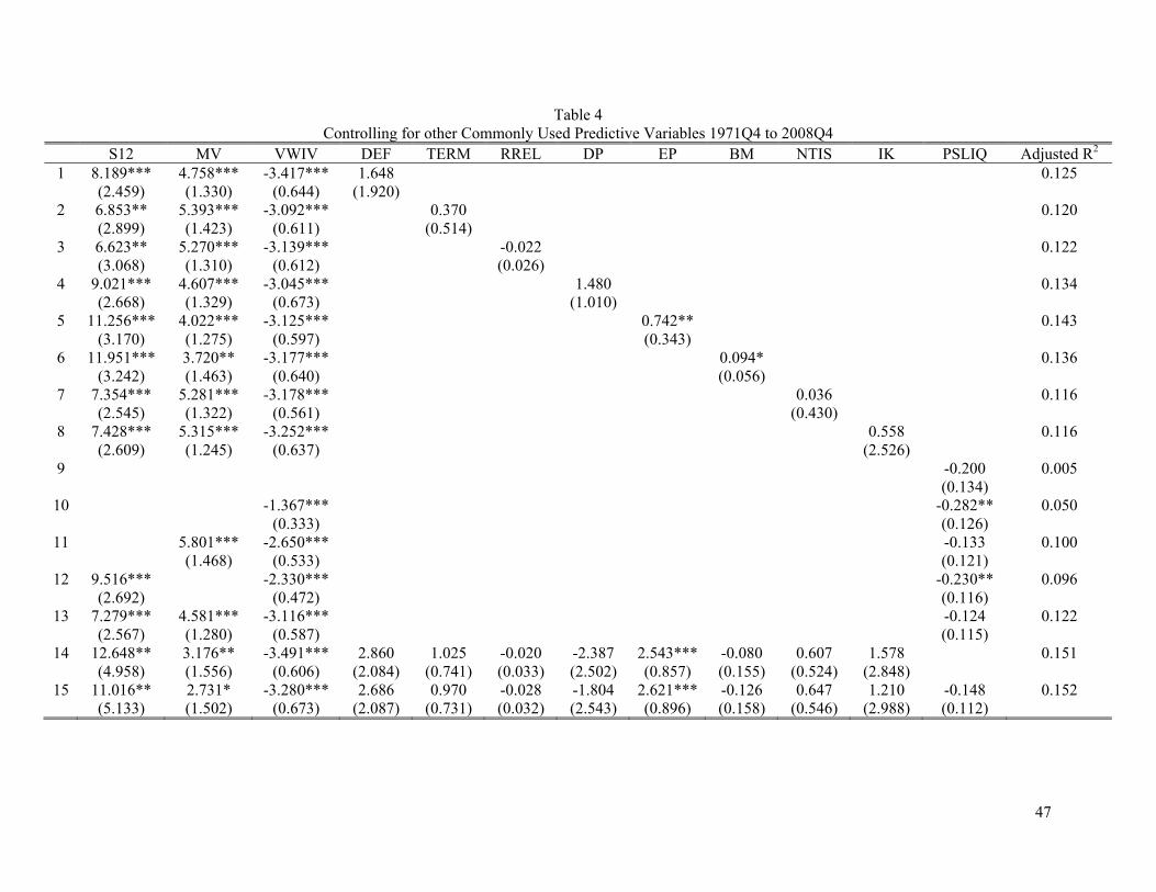
47  

Table 4 Controlling for other Commonly Used Predictive Variables 1971Q4 to 2008Q4

S12 MV VWIV DEF TERM RREL DP EP BM NTIS IK PSLIQ Adjusted R2

1 8.189*** (2.459)

4.758*** (1.330)

-3.417*** (0.644)

1.648 (1.920)

0.125

2 6.853** (2.899)

5.393*** (1.423)

-3.092*** (0.611)

0.370 (0.514)

0.120

3 6.623** (3.068)

5.270*** (1.310)

-3.139*** (0.612)

-0.022 (0.026)

0.122

4 9.021*** (2.668)

4.607*** (1.329)

-3.045*** (0.673)

1.480 (1.010)

0.134

5 11.256*** (3.170)

4.022*** (1.275)

-3.125*** (0.597)

0.742** (0.343)

0.143

6 11.951*** (3.242)

3.720** (1.463)

-3.177*** (0.640)

0.094* (0.056)

0.136

7 7.354*** (2.545)

5.281*** (1.322)

-3.178*** (0.561)

0.036 (0.430)

0.116

8 7.428*** (2.609)

5.315*** (1.245)

-3.252*** (0.637)

0.558 (2.526)

0.116

9 -0.200 (0.134)

0.005

10 -1.367*** (0.333)

-0.282** (0.126)

0.050

11 5.801*** (1.468)

-2.650*** (0.533)

-0.133 (0.121)

0.100

12 9.516*** (2.692)

-2.330*** (0.472)

-0.230** (0.116)

0.096

13 7.279*** (2.567)

4.581*** (1.280)

-3.116*** (0.587)

-0.124 (0.115)

0.122

14 12.648** (4.958)

3.176** (1.556)

-3.491*** (0.606)

2.860 (2.084)

1.025 (0.741)

-0.020 (0.033)

-2.387 (2.502)

2.543*** (0.857)

-0.080 (0.155)

0.607 (0.524)

1.578 (2.848)

0.151

15 11.016** (5.133)

2.731* (1.502)

-3.280*** (0.673)

2.686 (2.087)

0.970 (0.731)

-0.028 (0.032)

-1.804 (2.543)

2.621*** (0.896)

-0.126 (0.158)

0.647 (0.546)

1.210 (2.988)

-0.148 (0.112)

0.152

48  

Note: We report the OLS estimation results of forecasting one-quarter-ahead excess market returns using alternative measures of aggregate distress risk. S12 is average default scores over the 12-month horizon constructed using parameter estimate of the logit model reported in CHS (2010). MV is realized market variance. VWIV is average idiosyncratic variance. DEF is the yield spread between Baa- and Aaa-rated corporate bonds. TERM is the yield spared between 10-year Treasury bonds and 3-month Treasury bills. RREL is the stochastically detrended risk-free rate. DP is the dividend-price ratio. EP is the earnings-price ratio. BM is aggregate book-to-market equity ratio. NITS is the share of equities in new issuances. IK is the investment-capital ratio. PSLIQ is the liquidity measure proposed by Pastor and Stambaugh (2003). We report Newey-West standard errors in parentheses with four lags. ***, **, and * denote significance at the 1%, 5%, and 10% levels, respectively.

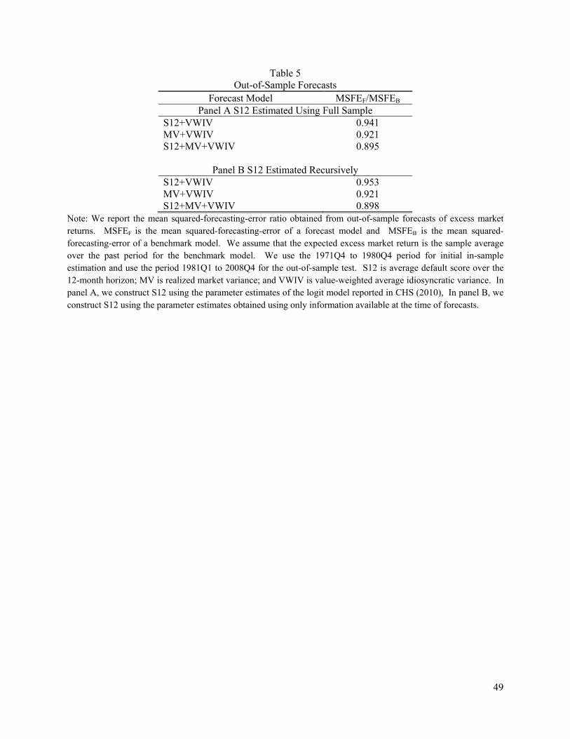
49  

Table 5 Out-of-Sample Forecasts

Forecast Model MSFEF/MSFEB

Panel A S12 Estimated Using Full Sample S12+VWIV 0.941 MV+VWIV 0.921 S12+MV+VWIV 0.895

Panel B S12 Estimated Recursively

S12+VWIV 0.953 MV+VWIV 0.921 S12+MV+VWIV 0.898

Note: We report the mean squared-forecasting-error ratio obtained from out-of-sample forecasts of excess market returns. MSFEF is the mean squared-forecasting-error of a forecast model and MSFEB is the mean squared-forecasting-error of a benchmark model. We assume that the expected excess market return is the sample average over the past period for the benchmark model. We use the 1971Q4 to 1980Q4 period for initial in-sample estimation and use the period 1981Q1 to 2008Q4 for the out-of-sample test. S12 is average default score over the 12-month horizon; MV is realized market variance; and VWIV is value-weighted average idiosyncratic variance. In panel A, we construct S12 using the parameter estimates of the logit model reported in CHS (2010), In panel B, we construct S12 using the parameter estimates obtained using only information available at the time of forecasts.

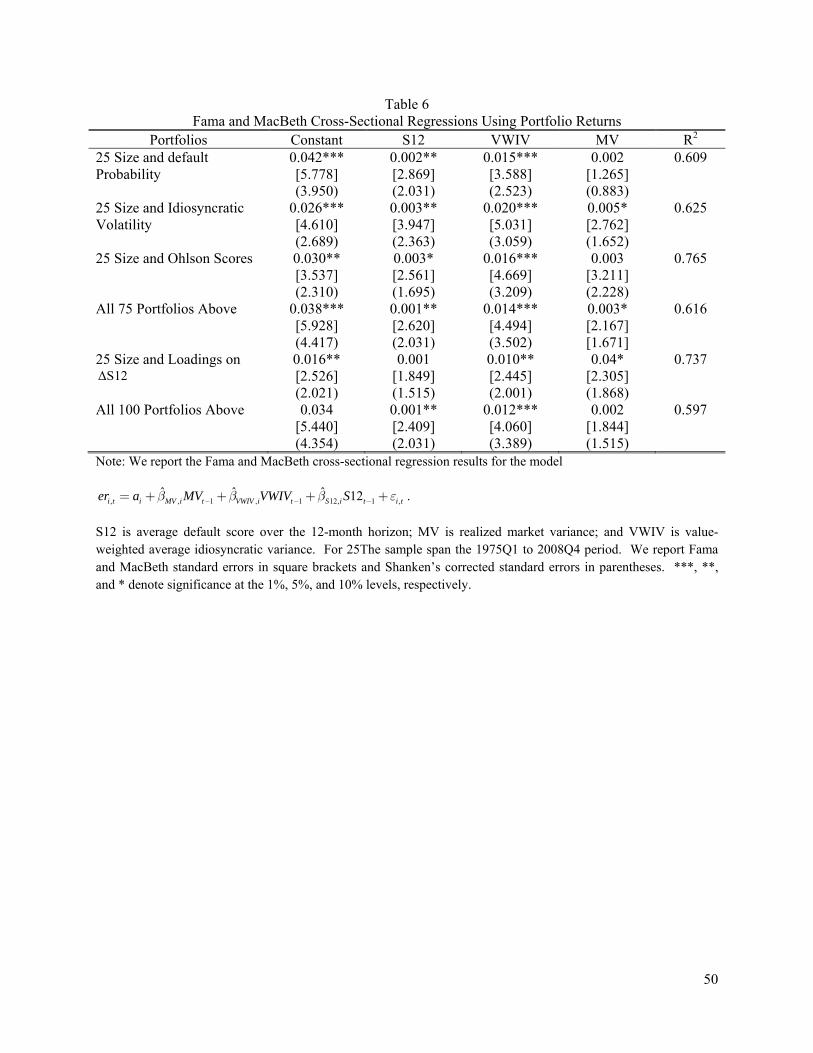
50  

Table 6 Fama and MacBeth Cross-Sectional Regressions Using Portfolio Returns

Portfolios Constant S12 VWIV MV R2

25 Size and default Probability

0.042*** [5.778] (3.950)

0.002** [2.869] (2.031)

0.015*** [3.588] (2.523)

0.002 [1.265] (0.883)

0.609

25 Size and Idiosyncratic Volatility

0.026*** [4.610] (2.689)

0.003** [3.947] (2.363)

0.020*** [5.031] (3.059)

0.005* [2.762] (1.652)

0.625

25 Size and Ohlson Scores 0.030** [3.537] (2.310)

0.003* [2.561] (1.695)

0.016*** [4.669] (3.209)

0.003 [3.211] (2.228)

0.765

All 75 Portfolios Above 0.038*** [5.928] (4.417)

0.001** [2.620] (2.031)

0.014*** [4.494] (3.502)

0.003* [2.167] [1.671]

0.616

25 Size and Loadings on ΔS12

0.016** [2.526] (2.021)

0.001 [1.849] (1.515)

0.010** [2.445] (2.001)

0.04* [2.305] (1.868)

0.737

All 100 Portfolios Above 0.034 [5.440] (4.354)

0.001** [2.409] (2.031)

0.012*** [4.060] (3.389)

0.002 [1.844] (1.515)

0.597

Note: We report the Fama and MacBeth cross-sectional regression results for the model

, , 1 , 1 12, 1 ,ˆ ˆ ˆ 12i t i MV i t VWIV i t S i t i ter a MV VWIV Sβ β β ε− − −= + + + + .

S12 is average default score over the 12-month horizon; MV is realized market variance; and VWIV is value-weighted average idiosyncratic variance. For 25The sample span the 1975Q1 to 2008Q4 period. We report Fama and MacBeth standard errors in square brackets and Shanken’s corrected standard errors in parentheses. ***, **, and * denote significance at the 1%, 5%, and 10% levels, respectively.

51  

Table 7 Decile Portfolios Sorted by Loadings on ΔS12

1 (lowest)

2 3 4 5 6 7 8 9 10 (highest)

1-10

Panel A Median Characteristics

,D iβ -1.076 -0.664 -0.487 -0.365 -0.264 -0.172 -0.081 0.013 0.118 0.318 -1.394

,M iβ 1.392 1.194 1.081 0.991 0.935 0.888 0.872 0.875 0.888 1.033 0.359 P12 0.057 0.050 0.048 0.047 0.047 0.046 0.045 0.044 0.043 0.043 0.014 SIZE 99 124 144 172 207 264 338 465 661 701 -601 BM 0.496 0.593 0.631 0.640 0.651 0.648 0.635 0.620 0.594 0.523 -0.027 IV 0.030 0.025 0.023 0.021 0.019 0.018 0.017 0.016 0.016 0.018 0.012 LEV 0.474 0.497 0.521 0.542 0.562 0.578 0.587 0.591 0.593 0.568 -0.094 ROE 1.854 2.216 2.398 2.548 2.631 2.699 2.747 2.782 2.850 2.823 -0.969 RET_1 0.011 0.010 0.010 0.010 0.010 0.009 0.010 0.010 0.009 0.009 0.002 RET_72 0.088 0.069 0.067 0.068 0.068 0.065 0.064 0.066 0.065 0.066 0.021

Panel B Equal-Weighted Excess Portfolio Returns

Excess Returns

0.680

0.923

0.946

1.015

1.032

0.909

0.909

0.805

0.696

0.593

0.087 (0.250)

Panel C Value-Weighted Excess Portfolio Returns

Excess Returns

0.588 0.759 0.837 0.756 0.786 0.706 0.660 0.739 0.498 0.405 0.182 (0.337)

Note: We sort stocks equally into decile portfolios by loadings on changes in aggregate distress risk, ,D iβ . Panel A reports the median characteristics of the

formation period. ,M iβ is loadings on market risk. P12 is the default probability in percentage over the 12-month horizon. SIZE is the market capitalization in

million dollars. BM is the book-to-market equity ratio. IV is idiosyncratic volatility. LEV is leverage calculated using book values of long-term debts and assets. ROE is the return on equity in percentage. RET_1 is stock return in the previous month. RET_72 is stock return over the past 7th month to 2nd month. Panel B reports the equal-weighted holding period portfolio return in percentage. Panel C reports the value-weighted holding period portfolio returns in percentage. The sample spans the January 1975 to December 2008 period.

52  

Table 8 Returns on Hedge Portfolios with Control for Idiosyncratic Volatility

Panel A Equal-Weighted Returns 1

(Lowest IV) 2 3 4 5

(Highest IV) Raw 0.449***

(0.134) 0.429*** (0.143)

0.385** (0.153)

0.119 (0.197)

-0.056 (0.198)

CAPM 0.386*** (0.134)

0.342** (0.142)

0.249* (0.148)

-0.070 (0.183)

-0.214 (0.193)

Fama and French Model 0.197* (.103)

0.141 (0.109)

0.164 (0.124)

-0.107 (0.159)

-0.162 (0.175)

Augmented Fama and French Model 0.234** (0.116)

0.160 (0.116)

0.179 (0.125)

-0.121 (0.162)

-0.242 (0.180)

Panel B Value-Weighted Returns

Raw 0.366** (0.179)

0.604*** (0.218)

0.465* (0.245)

0.142 (0.273)

0.117 (0.278)

CAPM 0.259 (0.181)

0.441** (0.210)

0.251 (0.233)

-0.097 (0.253)

-0.052 (0.273)

Fama and French 3 Factors 0.054 (0.156)

0.256 (0.184)

0.215 (0.202)

-0.185 (0.227)

-0.079 (0.260)

Augmented Fama and French Model 0.148 (0.158)

0.243 (0.184)

0.149 (0.211)

-0.215 (0.230)

-0.261 (0.259)

Note: we construct 25 portfolios sorted first by idiosyncratic volatility and then by loadings on changes in aggregate distress risk, ,D iβ using stocks with a price of $5 or higher. In particular, we first sort all stocks equally into

quintiles by idiosyncratic volatility and then sort stocks of each idiosyncratic volatility quintile equally into quintiles by ,D iβ . For each idiosyncratic volatility quintile, we construct a hedge portfolio that is long in quintile with the

smallest ,D iβ and short in quintile with the largest ,D iβ . The table reports returns on hedge portfolios for each

idiosyncratic volatility quintile from 1 (lowest idiosyncratic volatility) to 5 (highest idiosyncratic volatility). Panel A uses equal-weighted portfolio returns and panel B uses value-weighted portfolio returns. We report standard deviations or errors of portfolio returns in parentheses. We report raw returns, alpha from CAPM, alpha from the Fama and French (1996) 3-factor model, and alpha from the Fama and French (1996) 3-factor model augmented by the momentum factor. The sample span the January 1975 to December 2008 period. ***, **, and * denote significance at the 1%, 5%, and 10% levels, respectively.

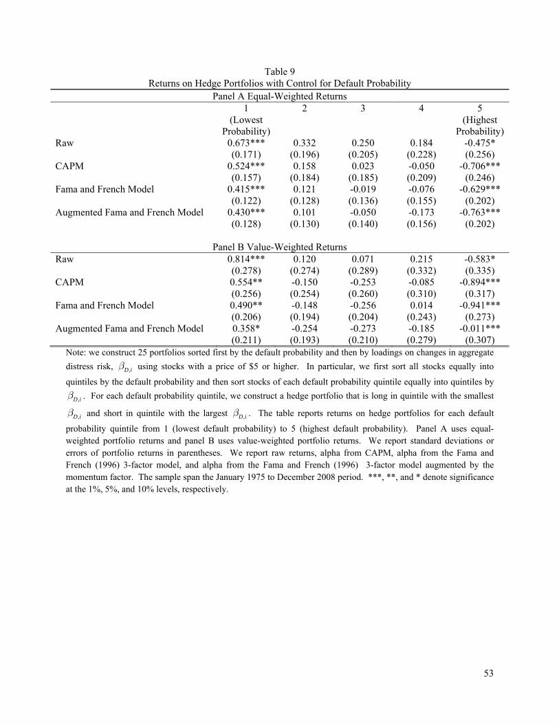
53  

Table 9 Returns on Hedge Portfolios with Control for Default Probability

Panel A Equal-Weighted Returns 1

(Lowest Probability)

2 3 4 5 (Highest

Probability) Raw 0.673***

(0.171) 0.332

(0.196) 0.250

(0.205) 0.184

(0.228) -0.475* (0.256)

CAPM 0.524*** (0.157)

0.158 (0.184)

0.023 (0.185)

-0.050 (0.209)

-0.706*** (0.246)

Fama and French Model 0.415*** (0.122)

0.121 (0.128)

-0.019 (0.136)

-0.076 (0.155)

-0.629*** (0.202)

Augmented Fama and French Model 0.430*** (0.128)

0.101 (0.130)

-0.050 (0.140)

-0.173 (0.156)

-0.763*** (0.202)

Panel B Value-Weighted Returns

Raw 0.814*** (0.278)

0.120 (0.274)

0.071 (0.289)

0.215 (0.332)

-0.583* (0.335)

CAPM 0.554** (0.256)

-0.150 (0.254)

-0.253 (0.260)

-0.085 (0.310)

-0.894*** (0.317)

Fama and French Model 0.490** (0.206)

-0.148 (0.194)

-0.256 (0.204)

0.014 (0.243)

-0.941*** (0.273)

Augmented Fama and French Model 0.358* (0.211)

-0.254 (0.193)

-0.273 (0.210)

-0.185 (0.279)

-0.011*** (0.307)

Note: we construct 25 portfolios sorted first by the default probability and then by loadings on changes in aggregate distress risk, ,D iβ using stocks with a price of $5 or higher. In particular, we first sort all stocks equally into

quintiles by the default probability and then sort stocks of each default probability quintile equally into quintiles by

,D iβ . For each default probability quintile, we construct a hedge portfolio that is long in quintile with the smallest

,D iβ and short in quintile with the largest ,D iβ . The table reports returns on hedge portfolios for each default

probability quintile from 1 (lowest default probability) to 5 (highest default probability). Panel A uses equal-weighted portfolio returns and panel B uses value-weighted portfolio returns. We report standard deviations or errors of portfolio returns in parentheses. We report raw returns, alpha from CAPM, alpha from the Fama and French (1996) 3-factor model, and alpha from the Fama and French (1996) 3-factor model augmented by the momentum factor. The sample span the January 1975 to December 2008 period. ***, **, and * denote significance at the 1%, 5%, and 10% levels, respectively.

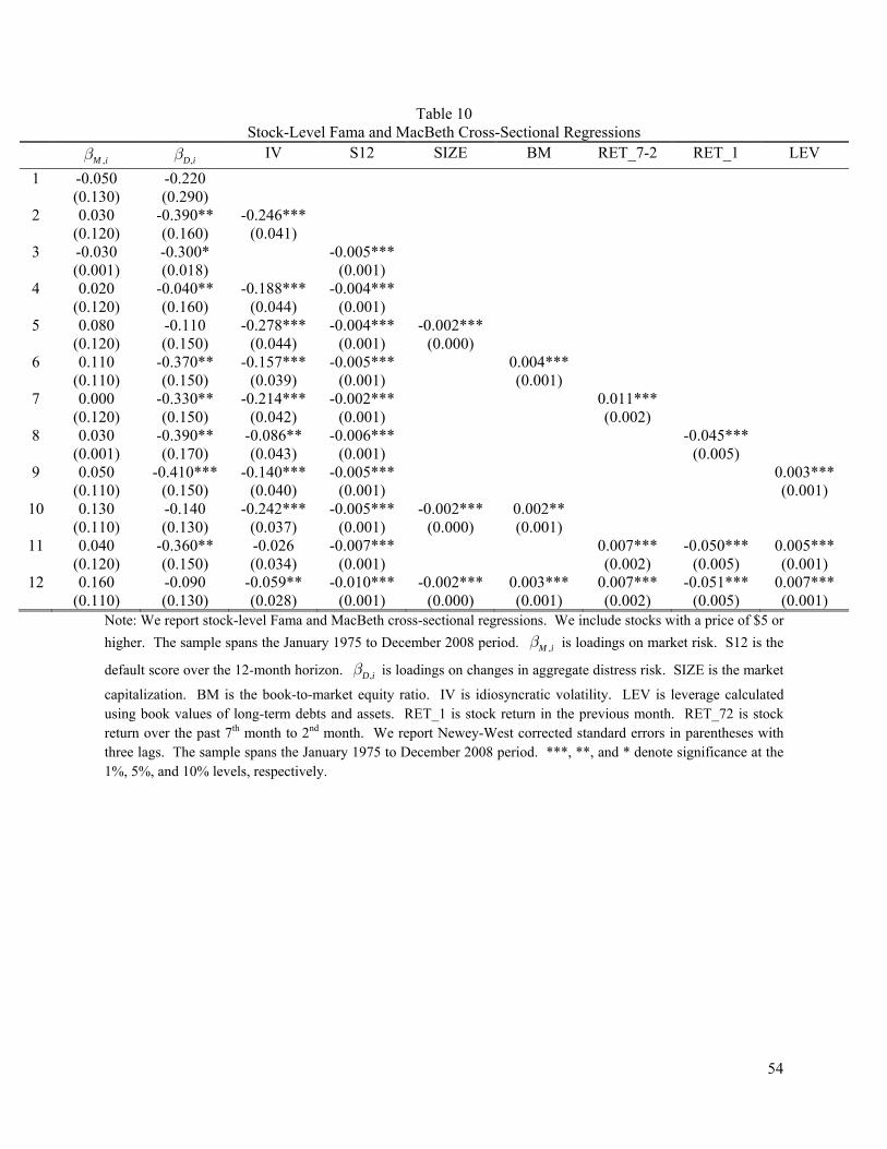
54  

Table 10 Stock-Level Fama and MacBeth Cross-Sectional Regressions

,M iβ ,D iβ IV S12 SIZE BM RET_7-2 RET_1 LEV 1 -0.050

(0.130) -0.220 (0.290)

2 0.030 (0.120)

-0.390** (0.160)

-0.246*** (0.041)

3 -0.030 (0.001)

-0.300* (0.018)

-0.005*** (0.001)

4 0.020 (0.120)

-0.040** (0.160)

-0.188*** (0.044)

-0.004*** (0.001)

5 0.080 (0.120)

-0.110 (0.150)

-0.278*** (0.044)

-0.004*** (0.001)

-0.002*** (0.000)

6 0.110 (0.110)

-0.370** (0.150)

-0.157*** (0.039)

-0.005*** (0.001)

0.004*** (0.001)

7 0.000 (0.120)

-0.330** (0.150)

-0.214*** (0.042)

-0.002*** (0.001)

0.011*** (0.002)

8 0.030 (0.001)

-0.390** (0.170)

-0.086** (0.043)

-0.006*** (0.001)

-0.045*** (0.005)

9 0.050 (0.110)

-0.410*** (0.150)

-0.140*** (0.040)

-0.005*** (0.001)

0.003*** (0.001)

10 0.130 (0.110)

-0.140 (0.130)

-0.242*** (0.037)

-0.005*** (0.001)

-0.002*** (0.000)

0.002** (0.001)

11 0.040 (0.120)

-0.360** (0.150)

-0.026 (0.034)

-0.007*** (0.001)

0.007*** (0.002)

-0.050*** (0.005)

0.005*** (0.001)

12 0.160 (0.110)

-0.090 (0.130)

-0.059** (0.028)

-0.010*** (0.001)

-0.002*** (0.000)

0.003*** (0.001)

0.007*** (0.002)

-0.051*** (0.005)

0.007*** (0.001)

Note: We report stock-level Fama and MacBeth cross-sectional regressions. We include stocks with a price of $5 or higher. The sample spans the January 1975 to December 2008 period. ,M iβ is loadings on market risk. S12 is the

default score over the 12-month horizon. ,D iβ is loadings on changes in aggregate distress risk. SIZE is the market

capitalization. BM is the book-to-market equity ratio. IV is idiosyncratic volatility. LEV is leverage calculated using book values of long-term debts and assets. RET_1 is stock return in the previous month. RET_72 is stock return over the past 7th month to 2nd month. We report Newey-West corrected standard errors in parentheses with three lags. The sample spans the January 1975 to December 2008 period. ***, **, and * denote significance at the 1%, 5%, and 10% levels, respectively.