A detailed report on

Acoustical Methods for Azimuth, Range and

Heading Estimation in Underwater Localization

The basic sequence of operation of the system can be explained as follows: an AUV (sender) emits two

acoustic ‘pings’ in sequence, first from the bow (front) end and next from the stern (rear) end. These two

pings constitute one sending event. Receivers (observers) which have the sender within their sensing

range would attempt to estimate the angle and the distance to each of the source upon receiving the

acoustic pings. These angles (sub-azimuths) and distances (sub-ranges) are then used to estimate the

compound azimuth, range and heading of the sending AUV, relative to each of the observers. These

azimuth, range and heading estimates are later used as components to assemble a pose vector which

contains the position information of the localized AUV.

The specific measurements and estimations carried out in this process are explained in the next sections,

starting with the angle and distance estimation for a single acoustic source. The methodology and basic

measurement schemes are described in detail along with identification of different classes of errors

affecting the estimated quantities. An analysis of how the uncertainties associated with the basic

measurements propagate towards uncertainties in the estimated quantities is given and a strategy for

minimizing the random errors of the estimates is also presented which contributes towards improving the

precision of the system. Later in the report describe how the sub-azimuths and sub-ranges are used to

derive the compound estimates for azimuth, range and heading in addition to an alternative scheme of

estimating heading and range independent of implicit sender-observer synchronization. Formulae

showing the relationship of the component quantities and their uncertainties with the uncertainty of the

compound quantities are also derived. These are used to analyze the behavior of the estimates with regard

to resolution and upper bounds for errors.

1.1 ANGLE ESTIMATION

TDOA measurement is the basis of hyperbolic localization and navigation schemes as well as many

bearing only tracking systems. TDOA, as the term suggests, is the difference of arrival times at two

receiver locations, of a signal transmitted from a third location. This quantity is then converted to an angle,

from which the source signal arrive towards the two receivers. In this context, the source signal consists

of an acoustically transmitted MLS signal and transmitters and receivers are projectors/pingers and

hydrophones.

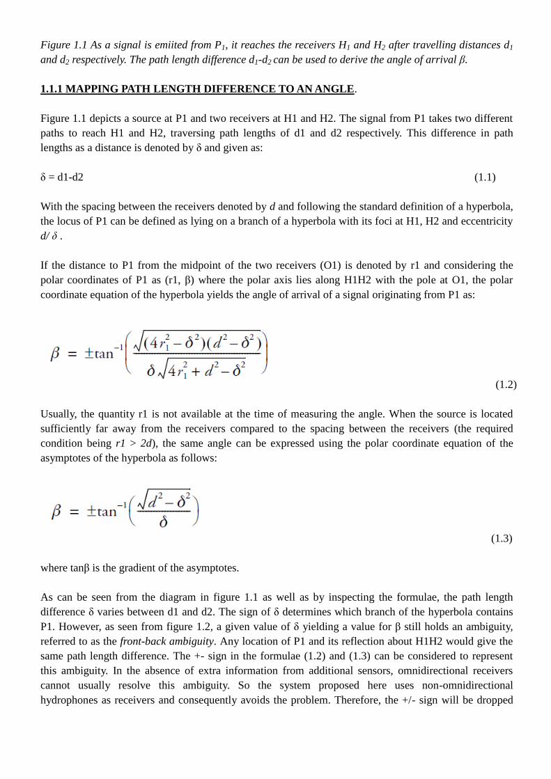
Figure 1.1 As a signal is emiited from P1, it reaches the receivers H1 and H2 after travelling distances d1

and d2 respectively. The path length difference d1-d2 can be used to derive the angle of arrival β.

1.1.1 MAPPING PATH LENGTH DIFFERENCE TO AN ANGLE.

Figure 1.1 depicts a source at P1 and two receivers at H1 and H2. The signal from P1 takes two different

paths to reach H1 and H2, traversing path lengths of d1 and d2 respectively. This difference in path

lengths as a distance is denoted by δ and given as:

δ = d1-d2 (1.1)

With the spacing between the receivers denoted by d and following the standard definition of a hyperbola,

the locus of P1 can be defined as lying on a branch of a hyperbola with its foci at H1, H2 and eccentricity

d/ δ .

If the distance to P1 from the midpoint of the two receivers (O1) is denoted by r1 and considering the

polar coordinates of P1 as (r1, β) where the polar axis lies along H1H2 with the pole at O1, the polar

coordinate equation of the hyperbola yields the angle of arrival of a signal originating from P1 as:

(1.2)

Usually, the quantity r1 is not available at the time of measuring the angle. When the source is located

sufficiently far away from the receivers compared to the spacing between the receivers (the required

condition being r1 > 2d), the same angle can be expressed using the polar coordinate equation of the

asymptotes of the hyperbola as follows:

(1.3)

where tanβ is the gradient of the asymptotes.

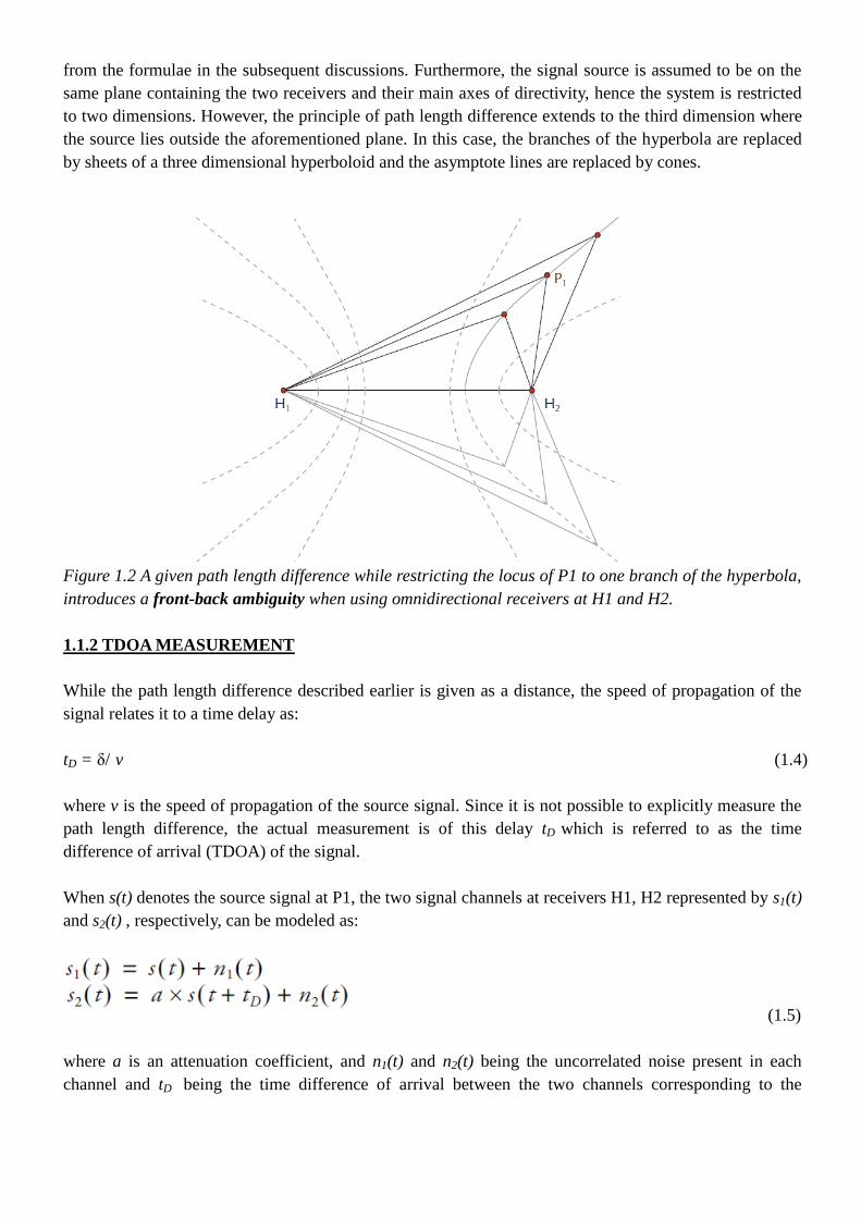
As can be seen from the diagram in figure 1.1 as well as by inspecting the formulae, the path length

difference δ varies between d1 and d2. The sign of δ determines which branch of the hyperbola contains

P1. However, as seen from figure 1.2, a given value of δ yielding a value for β still holds an ambiguity,

referred to as the front-back ambiguity. Any location of P1 and its reflection about H1H2 would give the

same path length difference. The +- sign in the formulae (1.2) and (1.3) can be considered to represent

this ambiguity. In the absence of extra information from additional sensors, omnidirectional receivers

cannot usually resolve this ambiguity. So the system proposed here uses non-omnidirectional

hydrophones as receivers and consequently avoids the problem. Therefore, the +/- sign will be dropped

from the formulae in the subsequent discussions. Furthermore, the signal source is assumed to be on the

same plane containing the two receivers and their main axes of directivity, hence the system is restricted

to two dimensions. However, the principle of path length difference extends to the third dimension where

the source lies outside the aforementioned plane. In this case, the branches of the hyperbola are replaced

by sheets of a three dimensional hyperboloid and the asymptote lines are replaced by cones.

Figure 1.2 A given path length difference while restricting the locus of P1 to one branch of the hyperbola,

introduces a front-back ambiguity when using omnidirectional receivers at H1 and H2.

1.1.2 TDOA MEASUREMENT

While the path length difference described earlier is given as a distance, the speed of propagation of the

signal relates it to a time delay as:

tD = δ/ v (1.4)

where v is the speed of propagation of the source signal. Since it is not possible to explicitly measure the

path length difference, the actual measurement is of this delay tD which is referred to as the time

difference of arrival (TDOA) of the signal.

When s(t) denotes the source signal at P1, the two signal channels at receivers H1, H2 represented by s1(t)

and s2(t) , respectively, can be modeled as:

(1.5)

where a is an attenuation coefficient, and n1(t) and n2(t) being the uncorrelated noise present in each

channel and tD being the time difference of arrival between the two channels corresponding to the

difference in path length .Transformation of the signal due to receiving and transmitting transducer

characteristics and the propagation medium is not explicitly modeled. These transformations do not affect

the measurement of tD when they are assumed to be common to both the channels.

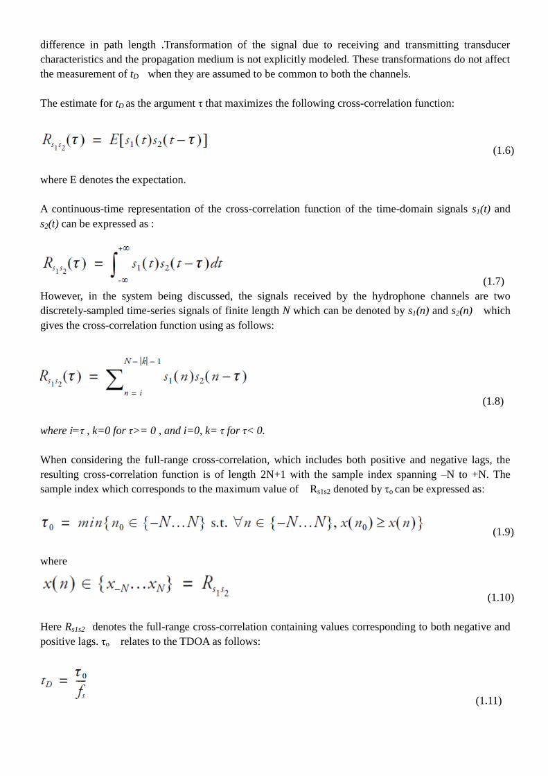
The estimate for tD as the argument τ that maximizes the following cross-correlation function:

(1.6)

where E denotes the expectation.

A continuous-time representation of the cross-correlation function of the time-domain signals s1(t) and

s2(t) can be expressed as :

(1.7)

However, in the system being discussed, the signals received by the hydrophone channels are two

discretely-sampled time-series signals of finite length N which can be denoted by s1(n) and s2(n) which

gives the cross-correlation function using as follows:

(1.8)

where i=τ , k=0 for τ>= 0 , and i=0, k= τ for τ< 0.

When considering the full-range cross-correlation, which includes both positive and negative lags, the

resulting cross-correlation function is of length 2N+1 with the sample index spanning –N to +N. The

sample index which corresponds to the maximum value of Rs1s2 denoted by τo can be expressed as:

(1.9)

where

(1.10)

Here Rs1s2 denotes the full-range cross-correlation containing values corresponding to both negative and

positive lags. τo relates to the TDOA as follows:

(1.11)

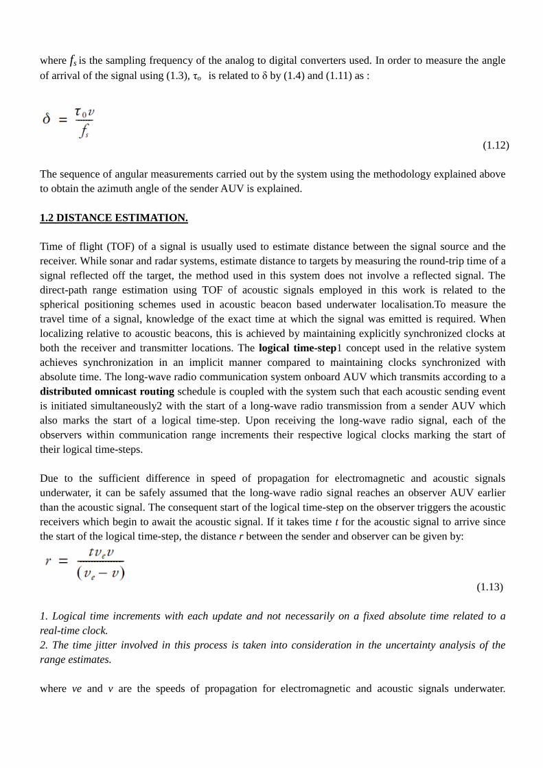
where fs is the sampling frequency of the analog to digital converters used. In order to measure the angle

of arrival of the signal using (1.3), τo is related to δ by (1.4) and (1.11) as :

(1.12)

The sequence of angular measurements carried out by the system using the methodology explained above

to obtain the azimuth angle of the sender AUV is explained.

1.2 DISTANCE ESTIMATION.

Time of flight (TOF) of a signal is usually used to estimate distance between the signal source and the

receiver. While sonar and radar systems, estimate distance to targets by measuring the round-trip time of a

signal reflected off the target, the method used in this system does not involve a reflected signal. The

direct-path range estimation using TOF of acoustic signals employed in this work is related to the

spherical positioning schemes used in acoustic beacon based underwater localisation.To measure the

travel time of a signal, knowledge of the exact time at which the signal was emitted is required. When

localizing relative to acoustic beacons, this is achieved by maintaining explicitly synchronized clocks at

both the receiver and transmitter locations. The logical time-step1 concept used in the relative system

achieves synchronization in an implicit manner compared to maintaining clocks synchronized with

absolute time. The long-wave radio communication system onboard AUV which transmits according to a

distributed omnicast routing schedule is coupled with the system such that each acoustic sending event

is initiated simultaneously2 with the start of a long-wave radio transmission from a sender AUV which

also marks the start of a logical time-step. Upon receiving the long-wave radio signal, each of the

observers within communication range increments their respective logical clocks marking the start of

their logical time-steps.

Due to the sufficient difference in speed of propagation for electromagnetic and acoustic signals

underwater, it can be safely assumed that the long-wave radio signal reaches an observer AUV earlier

than the acoustic signal. The consequent start of the logical time-step on the observer triggers the acoustic

receivers which begin to await the acoustic signal. If it takes time t for the acoustic signal to arrive since

the start of the logical time-step, the distance r between the sender and observer can be given by:

(1.13)

1. Logical time increments with each update and not necessarily on a fixed absolute time related to a

real-time clock.

2. The time jitter involved in this process is taken into consideration in the uncertainty analysis of the

range estimates.

where ve and v are the speeds of propagation for electromagnetic and acoustic signals underwater.

However, with the relatively short distances between the sender and receivers in a local neighborhood and

comparing the magnitudes of the quantities ve and v, it can be assumed that the long-wave radio signals

are transmitted between the neighboring vehicles instantaneously, which reduces (1.13) to:

(1.14)

where t can be expressed as the TOF of the acoustic signal.

1.2.1 MODIFIED MATCHED FILTER FOR TOF EXTRACTION.

A common approach used in echo signal detection is the use of a matched filter. The concept of matched

filter processing as a means for recovering a known waveform from a noisy signal is a well-known

process. In its conventional form, a noise-free replica of the original signal is cross-correlated with the

received signal channel to locate the return signal and thus extract the TOF. An improved ‘model based’

matched filter which uses a copy of the original signal which is convolved with the impulse response of

the transmission medium as the reference signal instead of a noise-free replica is also known. This

approach requires some a priori knowledge about the characteristics of the underwater environment in

which the AUVs operate in order to construct the impulse response.

The proposed system uses an actual received signal channel as the reference for cross-correlation. The

system initializes with a pre-recorded reference channel consisting of the MLS signal (which is used by

the system as the source signal waveform) which has been transmitted and received underwater via the

transducers used in the system. This technique compensates for the frequency distortions introduced by

the transducers as well as the transmission characteristics of the underwater medium. As the operation

progresses (when the AUV moves to areas with different underwater channel characteristics), this initial

reference signal can be replaced by a newly received signal which encompasses more up to date

characteristics of the transmission medium if and when the performance of the range estimation system

drops below a pre-set threshold value. This methodology presents a technique which can cope with

changing underwater channel characteristics without explicit measurements or a priori information about

the transmission medium.

The cross-correlation scheme described in the previous section is used for this ‘modified’ match filter as

well, where one signal channel is replaced by the reference signal in (1.8). Two cross-correlations are

performed to extract the TOF to each of the two receivers for each signal received from the sender AUV.

The diagram given in figure 1.3 shows the four TOFs associated with the two pings. The TOFs t11 and t12

are related to the front (bow) ping and the TOFs t21 and t22 are related to the rear (stern) ping. As

mentioned in the previous section, the long-wave radio signal emitted from the sender simultaneously

with the first acoustic ping is assumed to be received instantaneously by the observer, triggering the start

of the sending event. The subsequent TOFs are measured from this starting trigger. When implemented in

hardware, there is finite latency and timing jitter associated with detection of the long-wave signal and the

synchronized sending of the acoustic pings. If this synchronization latency of the receiving hardware is

denoted by tL, then the sample-domain latency τL is given by:

(1.15)

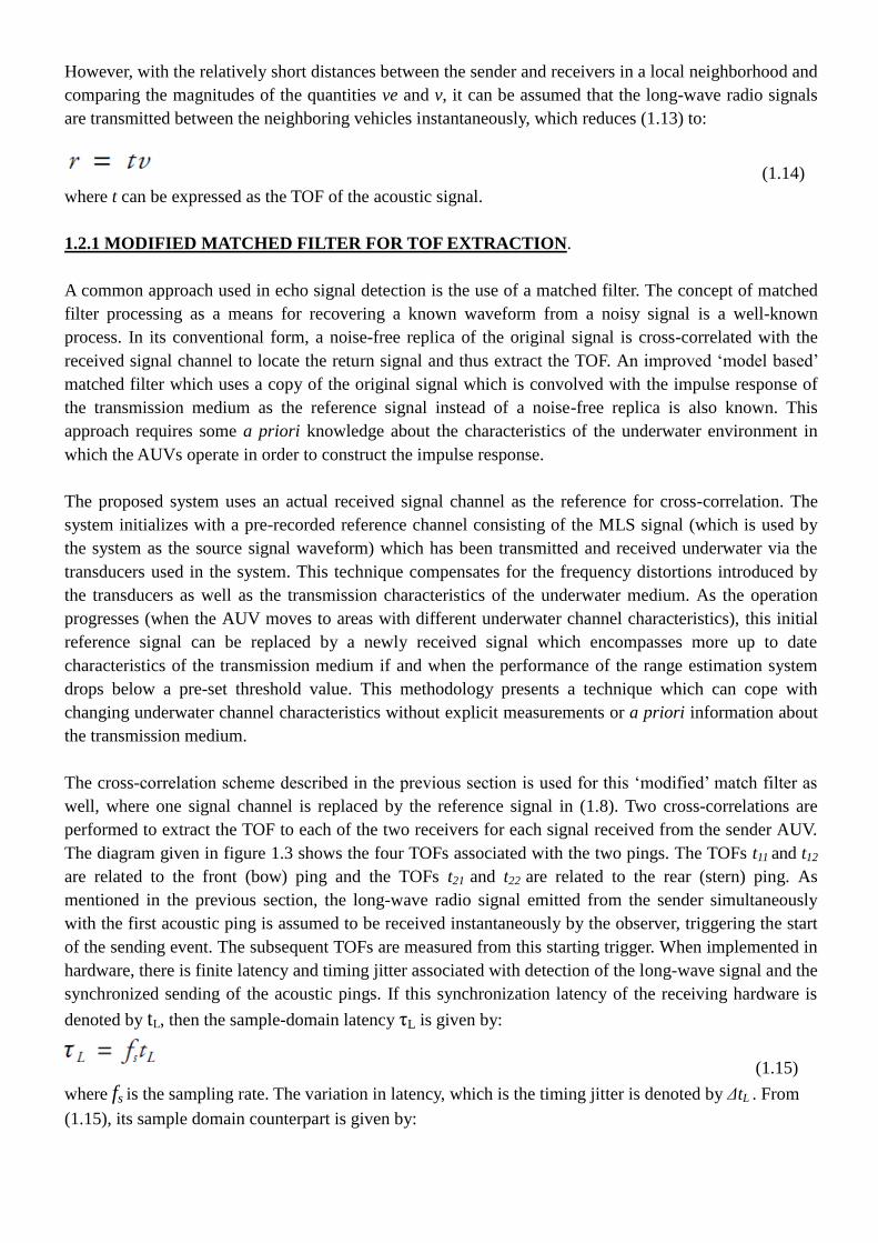
where fs is the sampling rate. The variation in latency, which is the timing jitter is denoted by ΔtL . From

(1.15), its sample domain counterpart is given by:

(1.16)

The above quantity will be included in the uncertainty analysis of the range estimates in the following

sections.

Without loss of generality, the range estimation will be explained in the next section using only the two

TOFs where the front (bow) ping is the source signal. For this purpose, the two sample-domain delays

obtained from (1.9) corresponding to the receivers H1, H2 are denoted by τ011

and τ012

with regard to a

signal transmitted from P1, (figure 1.4) the two TOFs and can be calculated as:

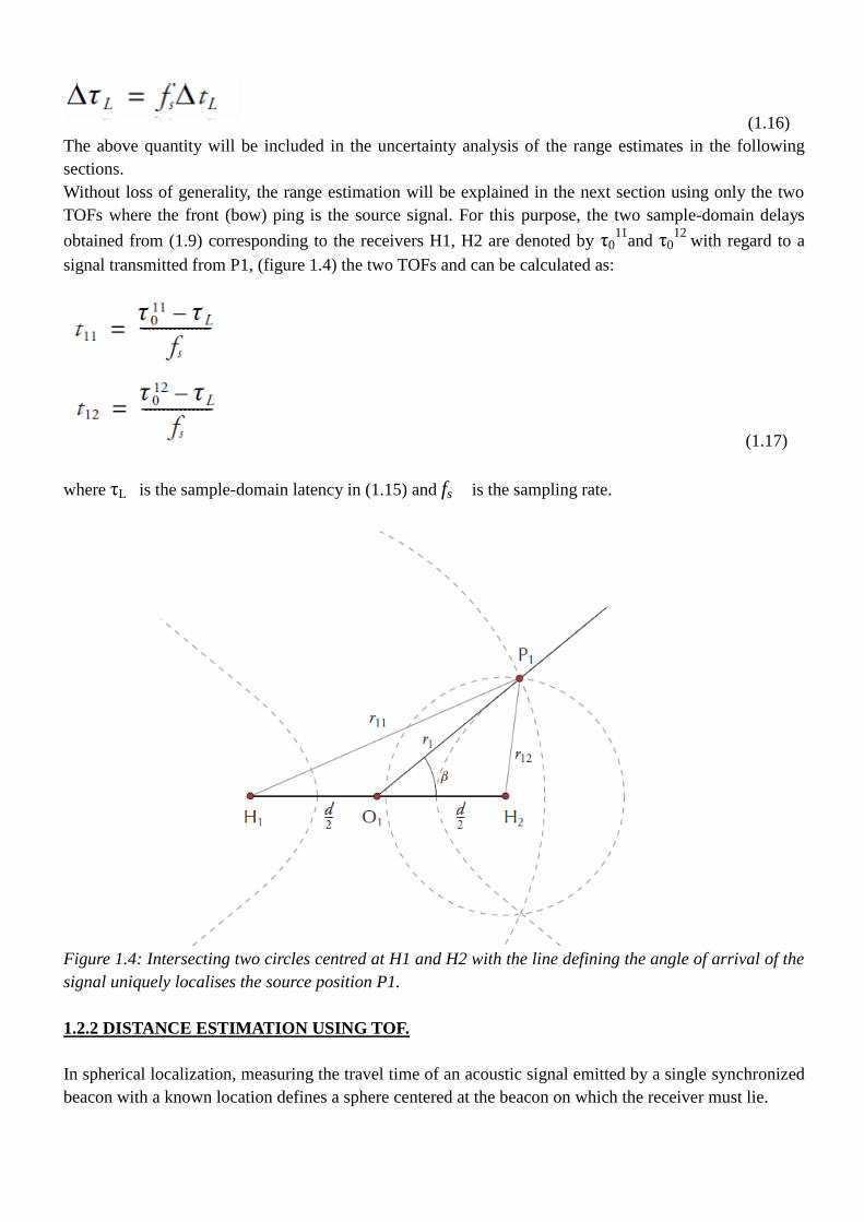
(1.17)

where τL is the sample-domain latency in (1.15) and fs is the sampling rate.

Figure 1.4: Intersecting two circles centred at H1 and H2 with the line defining the angle of arrival of the

signal uniquely localises the source position P1.

1.2.2 DISTANCE ESTIMATION USING TOF.

In spherical localization, measuring the travel time of an acoustic signal emitted by a single synchronized

beacon with a known location defines a sphere centered at the beacon on which the receiver must lie.

In the planar case considered in the system, the said sphere reduces to a circle. However, instead of the

multiple spheres (or circles in the planar case) needed to uniquely identify a position as done in traditional

spherical localization, using a single circle and its intersection with the line defining the angle of arrival

of the signal which was described in the previous sections, uniquely defines the position of the signal

source. In order to achieve better accuracy, two circles centered at the two receivers at H1 and H2 and the

line defining the angle of arrival is used as shown in figure 1.4. The radii of the circles centered at H1 and

H2 are denoted by r11(= P1H1) and r12(= P1H2) are obtained by substituting (1.17) in (1.14). The distance

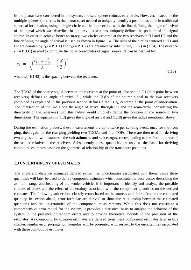
r1 (= P1O1) needed to complete the polar coordinates of signal source P1 can be derived by:

(1.18)

where d(=H1H2) is the spacing between the receivers.

The TDOA of the source signal between the receivers at the point of observation O1 (mid-point between

receivers) defines an angle of arrival β , while the TOFs of the source signal to the two receivers

combined as explained in the previous section defines a radius r1, centered at the point of observation.

The intersection of the line along the angle of arrival through O1 and the semi-circle (considering the

directivity of the receivers) with this radius would uniquely define the position of the source in two

dimensions. The equation in (1.3) gives the angle of arrival and (1.18) gives the radius mentioned above.

During the estimation process, these measurements are done twice per sending event, once for the front

ping, then again for the rear ping yielding two TDOAs and four TOFs. These are then used for deriving

two angles and two distances - the sub-azimuths and sub-ranges, corresponding to the front and rear of

the sender relative to the receivers. Subsequently, these quantities are used as the basis for deriving

compound estimates based on the geometrical relationship of the transducer positions.

1.3 UNCERTAINTNY OF ESTIMATES

The angle and distance estimates derived earlier has uncertainties associated with them. Since these

quantities will later be used to derive compound estimates which constitute the pose vector describing the

azimuth, range and heading of the sender vehicle, it is important to identify and analyze the possible

sources of errors and the effect of uncertainty associated with the component quantities on the derived

estimates. The following subsections classify errors based on the sources and their effect on the estimated

quantity. In section ahead, error formulae are derived to show the relationship between the estimated

quantities and the uncertainties of the component measurements. While this does not constitute a

comprehensive error model for the system, it provides a statistical basis to analyze the behavior of the

system in the presence of random errors and to provide theoretical bounds to the precision of the

estimates. As compound localization estimates are derived from these component estimates later in this

chapter, similar error propagation formulae will be presented with respect to the uncertainties associated

with these com-pound estimates.

RANDOM ERRORS

The primary measurements in each of the estimates are sample-domain delays, measured by detecting the

peak position after cross-correlation of pairs of discretized time-domain signal waveforms. By virtue of

this discretization, the position of the peak has an uncertainty of 0.5 samples which manifests itself as a

form of quantization error with an assumed uniform distribution. Apart from this, which affects the

TDOA measurement, the TOF measurement is also affected by the uncertainty introduced by

synchronization time-jitter mentioned earlier. The time-jitter is assumed to have a Gaussian distribution.

Both these sources of uncertainty lead to random errors, effects of which are non-deterministic, and

contribute to the lowering of precision of the estimated quantities. A strategy for reducing the impact of

these random errors is presented and discussed in later. There also is random measurement errors

associated with the constant quantities such as the speed of sound in water, sampling rate and the base

distance between hydrophones on the observer (and the separation between projectors on the sender) as

well.

SYSTEATIC ERRORS

In addition to these random errors, biases and variations associated with the constant quantities such as

the speed of sound in water , sampling rate , the base distance between hydrophones d on the observer

(and the separation between projectors on the sender) as well as the synchronization latency tL manifest

themselves as systematic errors in the estimation process. These errors affect the accuracy of the

estimated quantities. While it’s extremely difficult to individually identify the contributions of these

different errors to the final estimates, most of these systematic errors can be compensated by careful

calibration of the system and applying compound corrections.

ERRORS DUE TO LOW SNR.

Apart from the two forms of errors, another class of errors arises due to the deterioration of the signal-to-

noise ratio (SNR). Loss of signal could occur due to the source being out of the sensing range (radial or

angular) of the utilized transducers. In such situations, in the absence of a distinct waveform, the cross-

correlation is between channels containing ambient noise, which in the ideal cases would act as

uncorrelated noise. As a result, both forms of the cross-correlation peak detection (For TDOA and TOF

measurement) would return uniformly distributed random positions, affecting the accuracy of the

consequent estimates. In most real cases, the ambient noise appears weakly correlated on the two received

channels yielding a discernible peak near ‘0’ for the TDOA measurement, resulting in an angular estimate

in the vicinity of 90 degree(or 0 degree after the measuring conventions are applied as described). The

TOF measurement however is uninfluenced, by correlated noise in the absence of the signal of interest,

due to the matched filter processing and would continue to return random estimates.

Operating in highly cluttered, reverberant environments result in interference of the direct path signals by

reflected (multipath) signals. In such situations, without explicit identification and handling of the

situation, both the TDOA and TOF measurements would respond to the louder signal source which gives

a higher peak in the cross-correlogram (not necessarily the first arriving signal) which could lead to

inaccurate estimates for the source angle and range. With respect to the intended/ direct-path signal of

interest, the other signals (with the same wave form) due to colliding sending events and multipath can be

considered noise, which contributes to the lowering of the effective SNR. Though not always, in most

operating conditions, due to short-range propagation loss caused by acoustic spreading, the first arriving

signal would indeed be louder, yielding a higher peak.

Yet another form of interference could occur due to extraneous acoustic sources present in the

environment. Detrimental effects due to this last form of interference is largely avoided by the choice of

MLS signals as the source waveform due to their robustness against most such noise sources as discussed

in the previous chapter. However in the presence of intense broadband noise, due to the deterioration of

the SNR, the TDOA measurement could yield estimates which corresponds to the angular position of the

noise source rather than the signal source. The TOF measurements are usually unaffected by such

extraneous noise but could result in random errors caused by loss of cross-correlation peak height due to

severe deterioration of SNR.

1.3.1 PROPAGATION OF ERRORS.

The sources of random errors can be identified as the uncertainties associated with the sample-domain

delay estimations τo τo11

τo12

and the sample domain sender-observer synchronization latency τL,, given by

Δτo Δτo11

Δτo12

and ΔτL. Since the sample-domain delay estimates are obtained from the same cross-

correlation peak detection process, the associated uncertainties for the TDOA and TOF measurements are

assumed to be similar (Δτo =Δτo11

=Δτo12

) and represented by Δτ. The random measurement errors

associated with the quantities, d,v and fs and are denoted by Δ d, Δ v and Δ fs , and respectively.

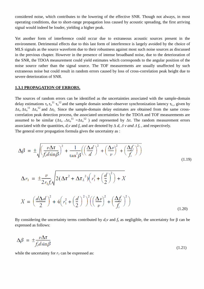
The general error propagation formula gives the uncertainty as :

(1.19)

(1.20)

By considering the uncertainty terms contributed by d,v and fs as negligible, the uncertainty for β can be

expressed as follows:

(1.21)

while the uncertainty for r1 can be expressed as:

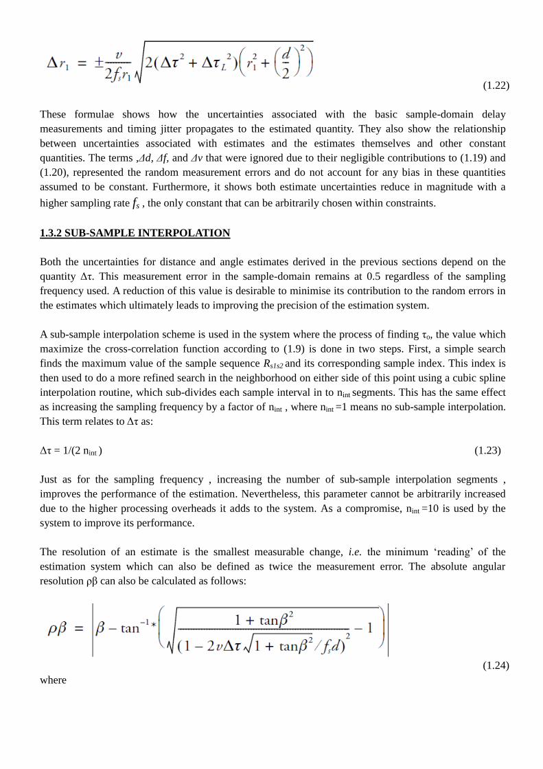
(1.22)

These formulae shows how the uncertainties associated with the basic sample-domain delay

measurements and timing jitter propagates to the estimated quantity. They also show the relationship

between uncertainties associated with estimates and the estimates themselves and other constant

quantities. The terms ,Δd, Δf, and Δv that were ignored due to their negligible contributions to (1.19) and

(1.20), represented the random measurement errors and do not account for any bias in these quantities

assumed to be constant. Furthermore, it shows both estimate uncertainties reduce in magnitude with a

higher sampling rate fs , the only constant that can be arbitrarily chosen within constraints.

1.3.2 SUB-SAMPLE INTERPOLATION

Both the uncertainties for distance and angle estimates derived in the previous sections depend on the

quantity Δτ. This measurement error in the sample-domain remains at 0.5 regardless of the sampling

frequency used. A reduction of this value is desirable to minimise its contribution to the random errors in

the estimates which ultimately leads to improving the precision of the estimation system.

A sub-sample interpolation scheme is used in the system where the process of finding τo, the value which

maximize the cross-correlation function according to (1.9) is done in two steps. First, a simple search

finds the maximum value of the sample sequence Rs1s2 and its corresponding sample index. This index is

then used to do a more refined search in the neighborhood on either side of this point using a cubic spline

interpolation routine, which sub-divides each sample interval in to nint segments. This has the same effect

as increasing the sampling frequency by a factor of nint , where nint =1 means no sub-sample interpolation.

This term relates to Δτ as:

Δτ = 1/(2 nint ) (1.23)

Just as for the sampling frequency , increasing the number of sub-sample interpolation segments ,

improves the performance of the estimation. Nevertheless, this parameter cannot be arbitrarily increased

due to the higher processing overheads it adds to the system. As a compromise, nint =10 is used by the

system to improve its performance.

The resolution of an estimate is the smallest measurable change, i.e. the minimum ‘reading’ of the

estimation system which can also be defined as twice the measurement error. The absolute angular

resolution ρβ can also be calculated as follows:

(1.24)

where

(1.25)

This function expands the range of the inverse tangent function from 0’-> 90’ to -90’-> 90’.

1.4 COMPOUND LOCALISATION ESTIMATES OF AZIMUTH θ, RANGE r AND HEADING α

Figure 1.5 : Azimuth θ, range r and heading angle α of sending AUV R2 wrt observing apparatus R1.

An acoustic sending event consists of two pings emitted by the sender AUV, first from the bow end and

the next from the stern end. Observers which have the sender within their sensing range would estimate

the angle and the distance to each of the two sources upon receiving the acoustic pings, resulting in two

sub-azimuth and four sub-range estimates. These are then used to derive the compound localisation

estimates of azimuth, range and heading of the sender relative to each of their body-fixed coordinate

frames of the observers.

Figure 1.5 illustrates observer (R1) measuring the azimuth, range and heading of AUV R2. These relative

measurements are based upon a polar system fixed on R1. The pole O1 is the mid-point of the line joining

the two receivers, H1 and H2 and the polar axis runs across the pole perpendicular to the line H1H2.

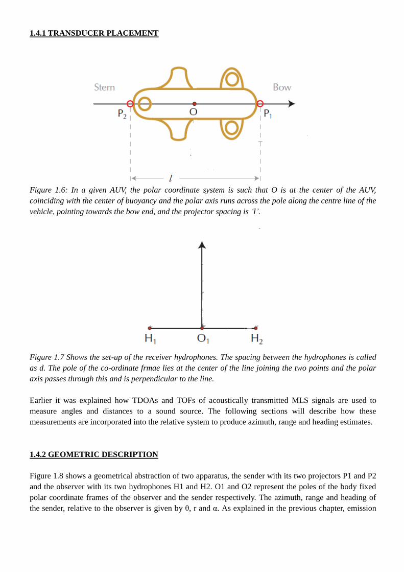
1.4.1 TRANSDUCER PLACEMENT

Figure 1.6: In a given AUV, the polar coordinate system is such that O is at the center of the AUV,

coinciding with the center of buoyancy and the polar axis runs across the pole along the centre line of the

vehicle, pointing towards the bow end, and the projector spacing is ‘l’.

Figure 1.7 Shows the set-up of the receiver hydrophones. The spacing between the hydrophones is called

as d. The pole of the co-ordinate frmae lies at the center of the line joining the two points and the polar

axis passes through this and is perpendicular to the line.

Earlier it was explained how TDOAs and TOFs of acoustically transmitted MLS signals are used to

measure angles and distances to a sound source. The following sections will describe how these

measurements are incorporated into the relative system to produce azimuth, range and heading estimates.

1.4.2 GEOMETRIC DESCRIPTION

Figure 1.8 shows a geometrical abstraction of two apparatus, the sender with its two projectors P1 and P2

and the observer with its two hydrophones H1 and H2. O1 and O2 represent the poles of the body fixed

polar coordinate frames of the observer and the sender respectively. The azimuth, range and heading of

the sender, relative to the observer is given by θ, r and α. As explained in the previous chapter, emission

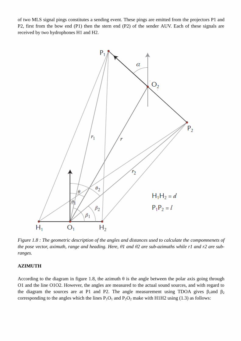
of two MLS signal pings constitutes a sending event. These pings are emitted from the projectors P1 and

P2, first from the bow end (P1) then the stern end (P2) of the sender AUV. Each of these signals are

received by two hydrophones H1 and H2.

Figure 1.8 : The geometric description of the angles and distances used to calculate the compomnenets of

the pose vector, aximuth, range and heading. Here, θ1 and θ2 are sub-azimuths while r1 and r2 are sub-

ranges.

AZIMUTH

According to the diagram in figure 1.8, the azimuth θ is the angle between the polar axis going through

O1 and the line O1O2. However, the angles are measured to the actual sound sources, and with regard to

the diagram the sources are at P1 and P2. The angle measurement using TDOA gives β1and β2

corresponding to the angles which the lines P1O1 and P2O2 make with H1H2 using (1.3) as follows:

(1.26)

where d=H1H2. δ1 and δ2 are the acoustic path length differences calculated according to (1.12), based

on the two TDOAs corresponding to the two MLS signals emitted from P1 and P2. Accordingly, the two

angles returned by (1.26) need to be transformed to θ1 and θ2 which are measured against the polar axis

instead of the line H1H2. This transformation is given by:

(1.27)

where the adjustment function is defined as:

(1.28)

which return the angles conforming to the convention.

This adjustment is required since (1.3) produces βi with the range βi ε(-180’-180’) when implemented

with the inverse tan function which considers the quadrant of the complex value x+iy where y/x=tanβ .

However, in the experimental implementation of the system, the range of (1.3) was limited to 0’-180’ due

to the directivity of the hydrophones used

The two angular measurements and obtained from (1.27) are combined to produce the azimuth estimate

according to the geometry of the diagram in figure 1.8 as follows:

(1.29)

RANGE

According to figure 1.8 the range r, which is the Euclidean distance between the poles of the coordinate

frames fixed to the sender and observer, is given as the length of line O1O2. However, as with the

azimuth measurement, the actual measurements are the distances to the sound sources P1 and P2 from

each of the receivers H1 and H2. If P1H1, P1H2 are denoted as r11,r12 , and P2H1, P2H2 as r21,r22 the

distances r1(P1O1) and r2(P2O1) can be calculated using (1.18) based on the TOF measurements given

earlier as follows:

(1.30)

where d is the distance between hydrophones on the observer. Once r1 and r2 are calculated, the range

can be calculated using the formula:

(1.31)

where l is the separation between the projectors on the sender vehicles.

HEADING

The relative heading α of the sender vehicle as seen by the observer vehicle can be estimated with the aid

of the component measurements θ1, θ2, r1 and r2 used earlier to derive the azimuth and the range. The

range adjusted heading can be expressed as:

(1.32)

where the θi values are given by (1.27) with the range from -180’ to 180’ and ri values are given by (1.30).

The adjustment function is same as the one in (1.28). While r1,r2 >= 0, by inspecting Figure 1.8, it is also

clear that they cannot both be zero at the same time, given the constrain that l > d.

1.4.3 REVERSE HYPERBOLIC LOCALISATION

The azimuth estimation presented in the previous sections is based on hyperbolic localization (TDOA

measurement) schemes while the range estimation is based on spherical localization (TOF measurement)

schemes. Overall, the source localization presented can be viewed as a hybrid approach. The heading

estimation relies on the azimuth and range as shown by (1.32). However, the range estimation and the

subsequent heading estimation require implicit synchronization between the sender and observer as with

traditional TOF based spherical localization schemes. This synchronization provided by the underlying

communication scheduling system enables the relative localization system to measure TOF as described

in section 1.2.

With the two sound sources at P1, P2 and the two receivers at H1, H2, a novel reverse hyperbolic scheme

was devised to calculate the range and heading which does not require a TOF measure-ment,

consequently eliminating the dependence on sender-observer synchronization.

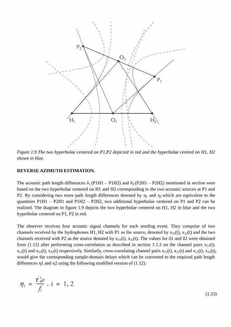
Figure 1.9 The two hyperbolae centered on P1,P2 depicted in red and the hyperbolae centred on H1, H2

shown in blue.

REVERSE AZIMUTH ESTIMATION.

The acoustic path length differences δ1 (P1H1 – P1H2) and δ2 (P2H1 – P2H2) mentioned in section were

based on the two hyperbolae centered on H1 and H2 corresponding to the two acoustic sources at P1 and

P2. By considering two more path length differences denoted by η1 and η2 which are equivalent to the

quantities P1H1 – P2H1 and P1H2 – P2H2, two additional hyperbolae centered on P1 and P2 can be

realized. The diagram in figure 1.9 depicts the two hyperbolae centered on H1, H2 in blue and the two

hyperbolae centered on P1, P2 in red.

The observer receives four acoustic signal channels for each sending event. They comprise of two

channels received by the hydrophones H1, H2 with P1 as the source, denoted by x11(t), x12(t) and the two

channels received with P2 as the source denoted by x21(t), x22(t). The values for δ1 and δ2 were obtained

from (1.12) after performing cross-correlation as described in section 1.1.2 on the channel pairs x11(t),

x12(t) and x21(t), x22(t) respectively. Similarly, cross-correlating channel pairs x11(t), x21(t) and x12(t), x22(t),

would give the corresponding sample-domain delays which can be converted to the required path length

differences η1 and η2 using the following modified version of (1.12):

(1.33)

where v is the speed of sound underwater, fs the sampling frequency of the analogue to digital converter

and τ’o1

, τ’o2

the sample-domain delays that maximize the respective cross-correlation functions.

Just as β1 and β2 defined the angles P1O1 and P2O1 made with H1H2, two new angles φ1 and φ2 can be

defined as the angles H1O2 and H2O2 makes with P1P2. These two angles can be obtained from a

slightly modified version of (1.26) using the path length differences η1 and η2 as follows:

(1.34)

where l is the separation between the two projectors P1,P2 and the modified sign function is defined as:

(1.35)

The angles returned from (1.34) has the range from -180’ to 180’ and can be combined to produce the

angle φ as:

(1.36)

This angle can be identified as the reverse azimuth of the sender vehicle or the azimuth of the observer

relative to the sender vehicle. The geometry of these quantities along with the measuring convention is

shown in figure 1.10

HEADING AND RANGE ESTIMATES BASED ON REVERSE AZIMUTH

According to the geometry shown in figure 1.10, an alternate relative heading (α’) of the sender with

respect to the observer can be given as:

(1.37)

The adjustment function is the same as above. The azimuth θ is as given by (1.29).

A new calculation for range based on the reverse azimuth φ and α’ derived above yields r’ as follows:

(1.38)

Figure 1.10: The geometric description of the new angles φ1, φ2, φ and their relationship to azimuth θ

and the alternate values for range r’ and heading α’.

As these alternate calculations are based on two hyperbolas, each with foci at P1 and P2, considering their

asymptotes which pass through H1 and H2, substituting these points in the polar coordinate equations for

O2H1 and O2H2 and adjusting for the measuring conventions, the separate range components can be

calculated using the following formula:

(1.39)

where the ‘+’ sign yield r’1 and the ‘-’ sign yield r’2. The variables have the following ranges: r’,l > 0, -

180’< θ1, α, θ < 180’ and the modified sign function is as defined as (1.35).

PROPERTIES OF ALTERNATE HEADING AND RANGE ESTIMATES.

The alternate heading and range estimates obtained above do not require sender-observer synchronization

or any knowledge of the sending time of the acoustic signal. This is due to the calculations being purely

based on TDOA measurements. This form of independence from the underlying scheduling system

provides an additional level of redundancy and increases the robustness of the relative localization system

against synchronization failures and timing drifts. This also facilitates a more fault tolerant outlier

rejection scheme with two independent estimates for the range and heading. However, in its current form,

the independence from sender-observer synchronization comes at a cost. The errors associated with the

alternate range are greater than those of the direct estimation. On the other hand, the errors associated

with the alternate heading are lower than its direct counterpart and these errors are not dependent on the

range as with the case of the direct heading estimation. The errors and associated resolution of the direct

and alternate estimates are discussed in the following sections.

1.4.4 ESTIMATION ERRORS AND RESOLUTION.

Earlier, the uncertainties associated with the angle and the distance estimates were presented in (1.21) and

(1.22). These angle and distance estimates were further developed to form the components of the pose

vector i.e. the azimuth, range, heading and the alternate versions of range and heading.

AZIMUTH

By applying the transformation given in (1.27), the angular uncertainties given by (1.21) can be expressed

as:

(1.40)

By applying the general error propagation formula to (4.33) and substituting for the sub-azi-muths errors

given above, the error for the main azimuth estimate is given as:

(1.41)

The error associated with azimuth is independent of the distance between the sender and the observer.

RANGE

The uncertainty for distance given by (1.22) can be extended to both sub-ranges r1 and r2 as:

(1.42)

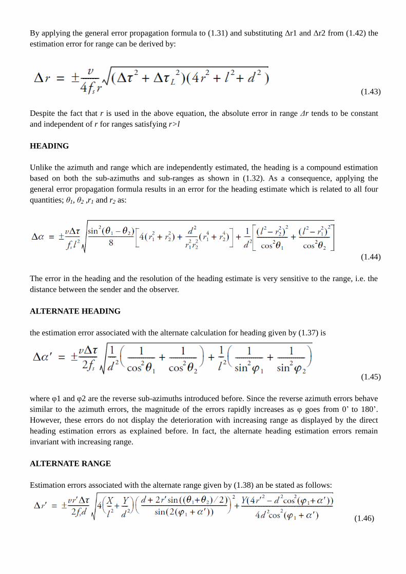
By applying the general error propagation formula to (1.31) and substituting Δr1 and Δr2 from (1.42) the

estimation error for range can be derived by:

(1.43)

Despite the fact that r is used in the above equation, the absolute error in range Δr tends to be constant

and independent of r for ranges satisfying r>l

HEADING

Unlike the azimuth and range which are independently estimated, the heading is a compound estimation

based on both the sub-azimuths and sub-ranges as shown in (1.32). As a consequence, applying the

general error propagation formula results in an error for the heading estimate which is related to all four

quantities; θ1, θ2 ,r1 and r2 as:

(1.44)

The error in the heading and the resolution of the heading estimate is very sensitive to the range, i.e. the

distance between the sender and the observer.

ALTERNATE HEADING

the estimation error associated with the alternate calculation for heading given by (1.37) is

(1.45)

where φ1 and φ2 are the reverse sub-azimuths introduced before. Since the reverse azimuth errors behave

similar to the azimuth errors, the magnitude of the errors rapidly increases as φ goes from 0’ to 180’.

However, these errors do not display the deterioration with increasing range as displayed by the direct

heading estimation errors as explained before. In fact, the alternate heading estimation errors remain

invariant with increasing range.

ALTERNATE RANGE

Estimation errors associated with the alternate range given by (1.38) an be stated as follows:

(1.46)

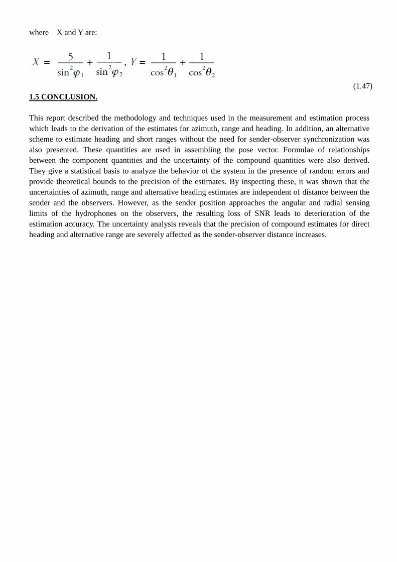
where X and Y are:

(1.47)

1.5 CONCLUSION.

This report described the methodology and techniques used in the measurement and estimation process

which leads to the derivation of the estimates for azimuth, range and heading. In addition, an alternative

scheme to estimate heading and short ranges without the need for sender-observer synchronization was

also presented. These quantities are used in assembling the pose vector. Formulae of relationships

between the component quantities and the uncertainty of the compound quantities were also derived.

They give a statistical basis to analyze the behavior of the system in the presence of random errors and

provide theoretical bounds to the precision of the estimates. By inspecting these, it was shown that the

uncertainties of azimuth, range and alternative heading estimates are independent of distance between the

sender and the observers. However, as the sender position approaches the angular and radial sensing

limits of the hydrophones on the observers, the resulting loss of SNR leads to deterioration of the

estimation accuracy. The uncertainty analysis reveals that the precision of compound estimates for direct

heading and alternative range are severely affected as the sender-observer distance increases.