Distance Distribution between Complex Network Nodes in

Distance Distribution between ComplexNetwork Nodes in Hyperbolic Space

Gregorio Alanis-Lobato*

Miguel A. Andrade-Navarro

Faculty of Biology, Johannes Gutenberg UniversitätInstitute of Molecular Biology, Ackermannweg 4, 55128 Mainz, Germany*[email protected]

In the emerging field of network science, a recent model proposes that ahyperbolic geometry underlies the network representation of complexsystems, shaping their topology and being responsible for their signa-ture features: scale invariance and strong clustering. Under this modelof network formation, points representing system components areplaced in a hyperbolic circle and connected if the distance betweenthem is below a certain threshold. Then the aforementioned propertiescome out naturally, as a direct consequence of the geometric principlesof the hyperbolic space containing the network. With the aim of provid-ing insights into the stochastic processes behind the structure of com-plex networks constructed with this model, the probability density forthe approximate hyperbolic distance between N points, distributedquasi-uniformly at random in a disk of radius R ~ lnN, is determinedin this paper, together with other density functions needed to derivethis result.

Introduction1.

Representing the dynamic relationships between complex system com-ponents as networks of interacting nodes has found applications in bi-ology [1], mathematics [2], technology [3], and even cosmology [4].Despite the apparent differences between these fields, the networksarising from their systems share many structural properties: scale-freenode degree distributions [5], self-similarity [6], and average graphgeodesics that grow logarithmically with the number of nodes andstrong clustering [7]. Moreover, these characteristics can also be pre-sent in geometric objects, like fractals or cellular automata [8–10],which has prompted the analysis of complex networks from a geomet-ric perspective [6, 8, 9, 11, 12].

Of special interest is a recent model of network growth that advo-cates for the geometric principles of hyperbolic space being responsi-ble for the emergence of the above-mentioned network signaturefeatures [13]. Thus, the formation of scale-free and strongly clustered

Complex Systems, 25 © 2016 Complex Systems Publications, Inc. https://doi.org/10.25088/ComplexSystems.25.3.223

mailto:[email protected]

networks is the result of an optimization process involving two vari-ables: node popularity and similarity between nodes.

Popularity reflects the property of a node to attract connectionsfrom others over time, and it is thus associated with a node’s senioritystatus in the system. On the other hand, nodes that are similar to eachother have a high likelihood of getting connected, regardless of theirrank. Dynamic generation of a network with this model can thusmimic the formation of, for example, social websites, where theconcepts of (social) popularity and similarity can be intuitively under-stood, but also of other types of networks, such as protein interac-tomes. There, popularity would correspond to the tendency of aprotein to establish more connections, which could correlate with aprotein having appeared at an early stage in evolution (seniority), andsimilarity could be in protein sequence or function. This is a goodexample of how very simple rules—in this case, link to the most popu-lar and similar node—result in complex behavior.

In the so-called ℍ2 model, which can be seen as the static version

of the popularity-similarity optimization discussed above [14, 15],nodes appear randomly in a hyperbolic disk with radius proportionalto the number of system components. Node pairs are then linked ifthey are hyperbolically close. The choice of this space to place nodesis a convenient way to abstract the tradeoff between popularity andsimilarity via the hyperbolic distance between them: popularity ismodeled by node radial coordinates and similarity by angular dis-tances between nodes. In this way, and due to the principles of hyper-bolic geometry, nodes that appear near the origin of the disk are morepopular/senior and have a higher probability of connecting to othernodes in the system, thus becoming the hubs of the network. In con-trast, nodes that appear on the periphery link only with nodes thatare really close (similar) to them [16].

One of the advantages of this model is that with the appropriatechoice of node density and hyperbolic disk radius, we can grow net-works with target node degree scaling exponent γ and average nodedegree and clustering coefficient, which can serve as null models fortesting hypotheses related to the formation of complex systems. As aresult, the goal of this work is to determine an analytical expressionfor the probability distribution of hyperbolic distances betweennodes, randomly placed in a hyperbolic disk. The resulting distribu-tion, which is based on an approximation of the hyperbolic distancebetween nodes, provides insights into the stochastic processes thatgive rise to the structure of complex networks and serves as a refer-ence for the type of node similarities needed to generate their scale-free and strongly clustered topologies.

224 G. Alanis-Lobato and M. A. Andrade-Navarro


Preliminaries2.

In this paper, the native representation of the hyperbolic space is

used, in which the two-dimensional hyperbolic space ℍ2, of constant

curvature K -ζ2, is contained in a Euclidean disk, and points areplaced at polar coordinates (r, θ). The results shown in Section 3 fo-cus on the case ζ 1. Even when the choice of different ζ changes theradius of the hyperbolic disk and scales distances between points in-

side it by a factor of 1 ζ, the network resulting from connecting

them remains the same [16].Note that while hyperbolic angles and distances from the origin of

the disk (i.e., radial coordinates) are equivalent to Euclidean anglesand distances from the origin, the length and area of a hyperbolic cir-

cle of radius r, L(r) 2π sinhr and A(r) 2πcosh(r) - 1, respec-

tively, expand exponentially with r and not polynomially like in theEuclidean scenario. Consequently, to distribute N points uniformly atrandom in a hyperbolic circle of radius R, angular coordinates

θ ∈ 0, 2π are sampled with the uniform density ρ(θ) 1 2π, and

radial coordinates r ∈ 0, R are sampled with the exponential density

ρ(r) sinh(r) coshR - 1 ≈ er-R (see Figure 1(a)). Note that if a pa-

rameter α ∈ 0, 1 is introduced in this expression, we can control the

density of points close to the origin of the hyperbolic circle (see equa-tion (1) and Figure 1(b)). This has a direct impact on the node degreedistribution of the network resulting from this modified node density,because, as mentioned in Section 1, nodes with small radial coordi-nates have a higher likelihood to be network hubs due to their prox-imity to all other nodes in the space:

ρ(r) ≈ αeα(r-R). (1)

Figure 1. (a) Uniform distribution of points in the hyperbolic circle, which cor-responds to setting α 1 in equation (1). (b) Quasi-uniform distribution ofpoints in the hyperbolic circle for two different values of α. Disk centers aremarked with a red cross and circle boundaries are depicted in gray.

Distance Distribution between Complex Network Nodes in Hyperbolic Space 225


Equation (1), which corresponds to a quasi-uniform distribution ofpoints in the hyperbolic circle of radius R, is the one used in the restof this paper.

To compute the distance between any two points (ri, θi) and rj, θj

in the hyperbolic disk of constant curvature -1, we can resort to thehyperbolic law of cosines (see equation (2) and Figure 2):

xi,j arcoshcosh(ri) coshrj - sinh(ri) sinhrj cosθi,j. (2)

θi,j π - π -θi-θj in equation (2) is the angle between points (i.e.,

their angular distance).For sufficiently large ri and rj, equation (2) can be closely approxi-

mated by equation (3), which is the expression for the hyperbolic dis-tance between points that is used in the rest of this paper:

xi,j ≈ ri + rj + 2 lnθi,j

2. (3)

Note that since xi,j ≥ 0, θi,j ≥ 2 e-ri-rj .

Figure 2. The hyperbolic distance xi,j between two points in the hyperbolic

disk can be computed with the help of the hyperbolic law of cosines (see equa-tion (2)) and closely approximated by equation (3).

Proof. Let us write equation (2) as:

coshxi,j cosh(ri) coshrj1 - tanh(ri) tanhrj cosθi,j.

Since limz→∞ tanh z 1 and ri and rj are large, we have:

coshxi,j ≈ cosh(ri)coshrj1 - cosθi,j cosh(ri) coshrj 2 sin2θi,j

2.



Using the definitions of cosh z e2z + 1 2ez (ez + e-z) 2:

e2xi,j + 1

2exi,j≈

eri + e-ri

2

erj + e-rj

22 sin2

θi,j

2.

Since ri and rj are large, e-ri and e-rj are very close to 0, which

gives:

e2xi,j - eri+rj sin2θi,j

2exi,j + 1 ≈ 0.

The above can be solved for exi,j as a quadratic equation, yielding:

exi,j ≈1

2eri+rj sin2

θi,j

21 ± 1 - 4e-2ri-2rj sin-4

θi,j

2.

Once again, since ri and rj are large, e-2ri-2rj → 0, making the nega-

tive term inside the squared root close to 0. As a result, consideringthe positive root only, the term in brackets is approximately 2, yield-ing:

exi,j ≈ eri+rj sin2θi,j

2.

Applying natural logarithms to both sides, the expression in equa-tion (3) is reached:

xi,j ≈ ri + rj + 2 ln sinθi,j

2≈ ri + rj + 2 ln

θi,j

2.

This completes the proof. □

In Section 3, the random variable Xi,j, the distance between two

random points in a hyperbolic circle, is considered, and its probability

density function (PDF) fXi,jxi,j ρxi,j is determined. This is

achieved with the help of two facts: (i) the PDF of a random variableis the derivative of its cumulative distribution function (CDF); and(ii)�the PDF of the sum of two random variables is the convolution oftheir individual PDFs. In the following, random variables Zq are de-

noted with capital letter and subscripted with the part q of equa-

tion�(3) being analyzed. FZqzq is the CDF of Zq and fZq

zq ρ(q) is

its PDF.



Determination of the Probability Distribution3.

Let us start by determining the PDF of the rightmost part of equa-tion�(3). To do so, we first need to determine the PDF ofθi,j π - π -θi-θj and, at the same time, the PDF of θi - θj. It is im-

portant to emphasize that the latter expression is different from θi,j.

While θi,j is the angular distance between points and is always ≥0,

θi - θj can be negative if θj > θi. The PDF of random variable Zθi-θj,

the difference of two random angles in the hyperbolic circle, corre-sponds to the following convolution (or cross-correlation in signal-processing terminology):

fZθi-θj

zθi-θj fZθi

zθi-θj+ θjfZθj

θjdθj.

Due to the domain of θj, the integration limits of this cross-correla-

tion must ensure that 0 ≤ zθi-θj+ θj ≤ 2π. This breaks the integral in

two pieces:

fZθi-θj

zθi-θj

0

2π-zθi-θjfZθi

zθi-θj+ θjfZθj

θjdθj, θj ≤ 2π - zθi-θj

-zθi-θj

2πfZθi

zθi-θj+ θjfZθj

θjdθj, θj ≥ -zθi-θj.

The solution of the integrals yields (see Figure 3(a)):

fZθi-θj

zθi-θj

1

2π+

zθi-θj

4π2, -2π ≤ zθi-θj

≤ 0

1

2π-

zθi-θj

4π2, 0 < zθi-θj

≤ 2π.

(4)

As a result, the PDF for random variable Zθi-θj

should be:

fZθi-θj

zθi-θj

2fZθi-θj

zθi-θj

1

π-

zθi-θj

2π2, 0 ≤ z

θi-θj≤ 2π.

To determine the PDF of Zπ-θi-θj π -Z

θi-θj, let us use its CDF:

FZπ-θi-θj zπ-θi-θj

Pπ -Zθi-θj

≤ zπ-θi-θj

1 - PZθi-θj

≤ π - zπ-θi-θj 1 - FZ

θi-θj π - zπ-θi-θj

1 - 0

π-zπ-θi-θj 1

π-

zθi-θj

2π2dz

θi-θj

1

2

zπ-θi-θj2

2π2+

zπ-θi-θj

π+

1

2.



Figure 3. The shape of the distributions derived for the rightmost term inequation (3): (a) the difference between the angles of two points in the hyper-bolic circle; (b) the angular distance between these points; and (c) the θi,j-

dependent correction applied to the sum of radial coordinates to approximatethe hyperbolic distance between these points. The red line corresponds to theanalytical expressions derived in this work (equations (4) through (6)), andthe histograms correspond to the actual distributions of pairwise differences,distances, and corrections between 1000 points placed at random accordingto α 1.

Note that the last expression is valid for -π ≤ zπ-θi-θj≤ π, and

that differentiation with respect to zπ-θi-θj finally gives:

fZπ-θi-θj zπ-θi-θj

1

2π1 +

zπ-θi-θj

π, -π ≤ zπ-θi-θj

≤ π.

Now, the PDF for random variable Zπ-θi-θj|| is simply the positive

part of fZπ-θi-θj zπ-θi-θj

plus its negative part, which yields:

fZπ-θi-θj ||zπ-θi-θj||

fZπ-θi-θj zπ-θi-θj||

+ fZπ-θi-θj -zπ-θi-θj||

1

π,

0 ≤ zπ-θi-θj||≤ π.

Let Θi,j π -Zπ-θi-θj|| be the random variable for the angle be-

tween two random points in the hyperbolic circle (i.e.,θi,j π - π -θi - θj ||). Using the CDF of Θi,j, we have:

FΘi,jθi,j Pπ -Zπ-θi-θj||

≤ θi,j 1 - PZπ-θi-θj||≤ π - θi,j

1 - FZπ-θi-θj ||π - θi,j 1 -

0

π-θi,j 1

πdzπ-θi-θj||

θi,j

π.



Differentiating with respect to θi,j, the resulting density is (see Fig-

ure 3(b)):

fΘi,jθi,j

1

π, 0 ≤ θi,j ≤ π. (5)

Thanks to equation (5), it is now possible to work out the PDF of

term 2 lnθi,j 2 in equation (3). Again, using the CDF method it is

straightforward to determine the PDF for random variable Zθij2:

fZθij2zθij2

2

π, 0 ≤ zθij2

≤ π.

With the help of the CDF method, the PDF of random variable

Zlnθij2 lnZθij2

is derived as follows:

FZlnθij2zlnθij2

PlnZθij2 ≤ zlnθij2

PZθij2≤ e

zlnθij2

FZθij2ezlnθij2

0

ezlnθij2 2

πdzθij2

2e

zlnθij2

π.

Differentiating with respect to zlnθij2:

fZlnθij2zlnθij2

2e

zlnθij2

π, zlnθij2

< lnπ

2.

Finally, it is not difficult to see that for the random variableC 2Zlnθij2

, the θij-dependent correction applied to the sum of ra-

dial coordinates in equation (3) is (see Figure 3(c)):

fC(c) ec/2

π, c < 2 ln

π

2. (6)

The next step of this analysis is to derive the PDF for the sum ofrandom variables Ri and Rj, which correspond to the radial coordi-

nates of two random points in the hyperbolic circle. The densities of

these variables are fRi αeα(ri-R) and fRj

αeαrj-R, respectively,

with constant R and ri, rj ≤ R. The PDF for random variable

Ri,j Ri +Rj is thus the convolution of the independent PDFs:

fRi,jri,j fRi

ri,j - rjfRjrjdrj.



To define the integration limits for the above convolution, considerthat rj ≤ R and thus ri,j - rj ≤ R too, which yields:

fRi,jri,j

ri,j-R

Rαeαri,j-rj-Rαeαrj-Rdrj

ri,j-R

Rα2eαri,j-2Rdrj α22R - ri,je

αri,j-2R, ri,j ≤ 2R.

(7)

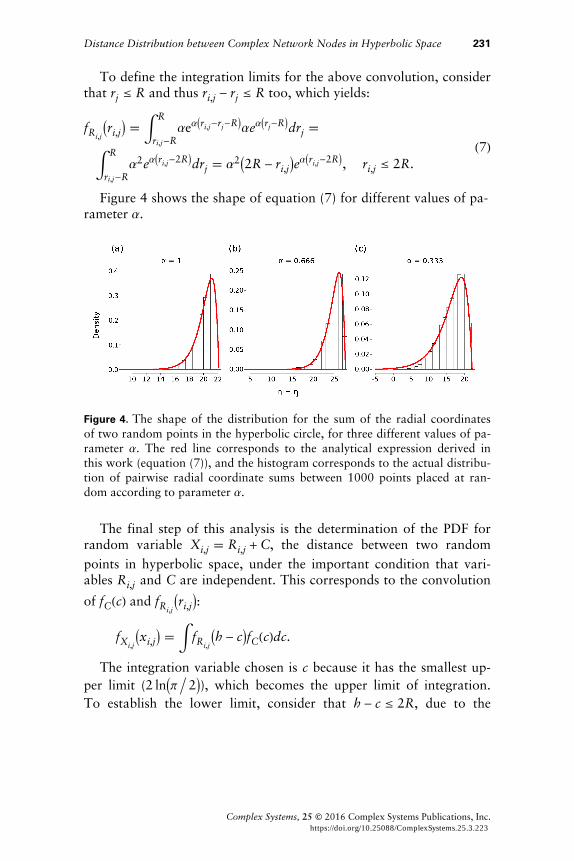
Figure 4 shows the shape of equation (7) for different values of pa-rameter α.

Figure 4. The shape of the distribution for the sum of the radial coordinatesof two random points in the hyperbolic circle, for three different values of pa-rameter α. The red line corresponds to the analytical expression derived inthis work (equation (7)), and the histogram corresponds to the actual distribu-tion of pairwise radial coordinate sums between 1000 points placed at ran-dom according to parameter α.

The final step of this analysis is the determination of the PDF forrandom variable Xi,j Ri,j +C, the distance between two random

points in hyperbolic space, under the important condition that vari-ables Ri,j and C are independent. This corresponds to the convolution

of fC(c) and fRi,jri,j:

fXi,jxi,j fRi,j

h - cfC(c)dc.

The integration variable chosen is c because it has the smallest up-

per limit (2 lnπ 2), which becomes the upper limit of integration.

To establish the lower limit, consider that h - c ≤ 2R, due to the



domain of fRi,j, which results in:

fXi,jxi,j

xi,j-2R

2 ln(π/2)α22R - xi,j + ce

αxi,j-m-2Rec/2

πdc

1

π1 - 2α2-2α2eαxi,j-2R-c+c2

2 + xi,j - 2αxi,j + 4α - 2R - c + 2αcxi,j-2R

2 ln(π/2).

(8)

Changing fXi,jxi,j to ρxi,j as defined in Section 2, the evaluation

of equation (8) in the given limits is finally equal to:

ρxi,j 2α2

π1 - 2α22exi,j2-R - eαxi,j-2R-2 ln(π/2)+ln(π/2)

2 + xi,j1 - 2α + 4α - 2 R + lnπ

2,

xi,j ≤ 2R + 2 lnπ

2.

(9)

Figure 5 shows the shape of equation (9) for different values ofparameter α, together with the histogram of the pairwise hyperbolicdistances between N 1000 points, distributed quasi-uniformly atrandom in the hyperbolic circle of radius R ~ lnN (see [3] for the ex-

act expression for R in the ℍ2 model for complex networks). Thanks

to a wxMaxima worksheet accompanying this work (see Section 4), itis possible to see that equation (9) is a valid PDF, since its integrationin the domain of xi,j equals 1.

Figure 5. The shape of the distribution for the hyperbolic distance between Nrandom points, quasi-uniformly distributed in the hyperbolic circle of radiusR ~ lnN for three different values of parameter α. The red line correspondsto the analytical expression derived in this work (equation (9)), and the his-togram corresponds to the actual distribution of pairwise distances between1000 points placed at random according to parameter α.



Note that although equation (3) closely approximates equation (2),a consequence of the assumption of large ri and rj that leads to equa-

tion (3) is that a fraction of equation (9)’s domain is negative (see Fig-ure 5), which is not expected from a distance distribution. Thisshould not represent a problem for the construction of networks with

scaling exponent γ ∈ 2, 3, the range that is typically observed in real

systems [13]. The reason why this is the case is that the choice of α im-pacts the network’s degree exponent γ 2α + 1 [16]. When γ ≥ 2,

that is, α ≥ 1 2, the probability that nodes have small radial coordi-

nates is very low, and even if their angular distances are small, thesum of their radial coordinates is big enough for equation (3) to be≥ 0 (see Figures 1(a), 1(b) left, 4(a, b), and 5(a, b)). However, if

α ∈ 0, 1 2, nodes are closer to the center of the hyperbolic disk,

thus increasing the probability of observing negative distances (see Fig-ures 1(b) right, 4(c), and 5(c)).

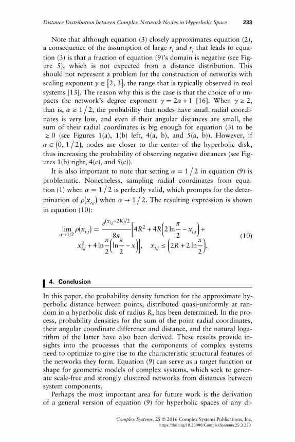
It is also important to note that setting α 1 2 in equation (9) is

problematic. Nonetheless, sampling radial coordinates from equa-

tion�(1) when α 1 2 is perfectly valid, which prompts for the deter-

mination of ρxi,j when α → 1 2. The resulting expression is shown

in equation (10):

limα→1/2

ρxi,j exi,j-2R2

8π4R2 + 4R 2 ln

π

2- xi,j +

xi,j2 + 4 ln

π

2ln

π

2- x , xi,j ≤ 2R + 2 ln

π

2.

(10)

Conclusion4.

In this paper, the probability density function for the approximate hy-perbolic distance between points, distributed quasi-uniformly at ran-dom in a hyperbolic disk of radius R, has been determined. In the pro-cess, probability densities for the sum of the point radial coordinates,their angular coordinate difference and distance, and the natural loga-rithm of the latter have also been derived. These results provide in-sights into the processes that the components of complex systemsneed to optimize to give rise to the characteristic structural features ofthe networks they form. Equation (9) can serve as a target function orshape for geometric models of complex systems, which seek to gener-ate scale-free and strongly clustered networks from distances betweensystem components.

Perhaps the most important area for future work is the derivationof a general version of equation (9) for hyperbolic spaces of any di-



mension D ≥ 2. In that case, nodes would be inside a hyperbolicsphere, and their position would be described by a radial coordinate rand D - 1 angular coordinates Θ. Furthermore, equation (1) wouldhave to change and represent a volume density rather than a planarone. Notwithstanding that such considerations are quite interesting,

networks lying on ℍD spaces (D ≫ 2) have zero clustering in the limitof large N [15]. In contrast, real-world networks are strongly clus-

tered, just like those generated by the ℍ2 model, making them more re-alistic and more suitable for the study of the dynamics underlying theformation of complex systems.

Despite the fact that the most representative models of complex net-work formation are based on very simple rules [5, 7, 13, 16], networkconstruction subject to optimization constraints or automata rules is arelatively fertile field in network science. Developments in the analysisof networks derived from cellular automata [17], network automata[18], trinet automata [19], and simple optimization [20] call forgreater efforts aimed at understanding the relationships between sim-ple computational systems and real-world networks.

A wxMaxima worksheet for the solution of cumbersome integralsin this paper and R code for the density, distribution, and quantilefunctions derived from the analytical expression determined are avail-able at http://www.greg-al.info/code, together with a Wolfram Note-book with interactive plots of the main PDFs derived. R code for thegeneration of quasi-uniform point densities in hyperbolic space isavailable at the same link.

Acknowledgments

The authors would like to thank Ron Gordon for a post inhttp://math.stackexchange.com that helped with the proof associatedto equation (3).

References

[1] M. Vidal, M. E. Cusick, and A.-L. Barabási, “Interactome Networksand Human Disease,” Cell, 144(6), 2011 pp. 986–998.doi:10.1016/j.cell.2011.02.016.

[2] G. García-Pérez, M. Á. Serrano, and M. Boguñá, “Complex Architec-ture of Primes and Natural Numbers,” Physical Review E, 90(2), 2014022806. doi:10.1103/PhysRevE.90.022806.



http://www.greg-al.info/code

http://math.stackexchange.com/

http://dx.doi.org/10.1016/j.cell.2011.02.016

http://dx.doi.org/10.1103/PhysRevE.90.022806

[3] M. Boguñá, F. Papadopoulos, and D. Krioukov, “Sustaining the Internetwith Hyperbolic Mapping,” Nature Communications, 1, 2010 62.doi:10.1038/ncomms1063.

[4] D. Krioukov, M. Kitsak, R. S. Sinkovits, D. Rideout, D. Meyer, andM. Boguñá, “Network Cosmology,” Scientific Reports, 2, 2012 793.doi:10.1038/srep00793.

[5] A.-L. Barabási and R. Albert, “Emergence of Scaling in Random Net-works,” Science, 286(5439), 1999 pp. 509–512.doi:10.1126/science.286.5439.509.

[6] M. Á. Serrano, D. Krioukov, and M. Boguñá, “Self-Similarity of Com-plex Networks and Hidden Metric Spaces,” Physical Review Letters,100, 2008 078701. doi:10.1103/PhysRevLett.100.078701.

[7] D. J. Watts and S. H. Strogatz, “Collective Dynamics of ‘Small-World’Networks,” Nature, 393(6684), 1998 pp. 440–442. doi:10.1038/30918.

[8] K.-I. Goh, G. Salvi, B. Kahng, and D. Kim, “Skeleton and Fractal Scal-ing in Complex Networks,” Physical Review Letters, 96(1), 2006018701. doi:10.1103/PhysRevLett.96.018701.

[9] C. Song, S. Havlin, and H. A. Makse, “Origins of Fractality inthe Growth of Complex Networks,” Nature Physics, 2(4), 2006pp.�275–281. doi:10.1038/nphys266.

[10] M. Schaller and K. Svozil, “Scale-Invariant Cellular Automata and Self-Similar Petri Nets,” The European Physical Journal B, 69(2), 2009pp.�297–311. doi:10.1140/epjb/e2009-00147-x.

[11] T. Aste, T. Di Matteo, and S. T. Hyde, “Complex Networks on Hyper-bolic Surfaces,” Physica A: Statistical Mechanics and Its Applications,346(1–2), 2005 pp. 20–26. doi:10.1016/j.physa.2004.08.045.

[12] T. Aste, R. Gramatica, and T. Di Matteo, “Exploring Complex Net-works via Topological Embedding on Surfaces,” Physical Review E,86(3), 2012 036109. doi:10.1103/PhysRevE.86.036109.

[13] F. Papadopoulos, M. Kitsak, M. Á. Serrano, M. Boguñá, and D. Kri-oukov, “Popularity versus Similarity in Growing Networks,” Nature,489(7417), 2012 pp. 537–540. doi:10.1038/nature11459.

[14] D. Krioukov and M. Ostilli, “Duality between Equilibrium and Grow-ing Networks,” Physical Review E, 88(2), 2013 022808.doi:10.1103/PhysRevE.88.022808.

[15] L. Ferretti, M. Cortelezzi, and M. Mamino, “Duality between Preferen-tial Attachment and Static Networks on Hyperbolic Spaces,” Euro-physics Letters, 105(3), 2014 38001.http://stacks.iop.org/0295-5075/105/i=3/a=38001.

[16] D. Krioukov, F. Papadopoulos, M. Kitsak, A. Vahdat, and M. Boguñá,“Hyperbolic Geometry of Complex Networks,” Physical Review E,82(3), 2010 036106. doi:10.1103/PhysRevE.82.036106.



http://dx.doi.org/doi:10.1038/ncomms1063

http://dx.doi.org/10.1038/srep00793

http://dx.doi.org/10.1126/science.286.5439.509

http://dx.doi.org/10.1103/PhysRevLett.100.078701

http://dx.doi.org/10.1038/30918

http://dx.doi.org/10.1103/PhysRevLett.96.018701

http://dx.doi.org/10.1038/nphys266

http://dx.doi.org/10.1140/epjb/e2009-00147-x

http://dx.doi.org/10.1016/j.physa.2004.08.045


http://dx.doi.org/10.1038/nature11459


http://stacks.iop.org/0295-5075/105/i=3/a=38001


[17] Y. Kayama, “Complex Networks Derived from Cellular Automata.”arxiv.org/abs/1009.4509.

[18] D. M. D. Smith, J.-P. Onnela, C. F. Lee, M. D. Fricker, and N. F. John-son, “Network Automata: Coupling Structure and Function in DynamicNetworks,” Advances in Complex Systems, 14(3), 2011 pp. 317–339.doi:10.1142/S0219525911003050.

[19] R. Southwell, H. Jianwei, and C. Cannings, “Complex Networks fromSimple Rules,” Complex Systems, 22(2), 2013 pp. 151–173.http://www.complex-systems.com/pdf/22-2-2.pdf.

[20] B. Zheng, H. Wu, L. Kuang, J. Qin, W. Du, J. Wang, and D. Li, “A Sim-ple Model Clarifies the Complicated Relationships of Complex Net-works,” Scientific Reports, 4, 2014 6197. doi:10.1038/srep06197.



http://arxiv.org/abs/1009.4509

http://dx.doi.org/10.1142/S0219525911003050

http://www.complex-systems.com/pdf/22-2-2.pdf

http://dx.doi.org/10.1038/srep06197

Documents

Distance Distribution between Complex Network Nodes in