Embed Size (px)
Citation preview

Distance and Similarity Measures
Bamshad Mobasher
DePaul University

Distance or Similarity Measuresi Many data mining and analytics tasks involve the comparison of
objects and determining their similarities (or dissimilarities)4 Clustering4 Nearest-neighbor search, classification, and prediction4 Characterization and discrimination4 Automatic categorization4 Correlation analysis
i Many of todays real-world applications rely on the computation similarities or distances among objects4 Personalization4 Recommender systems4 Document categorization4 Information retrieval4 Target marketing
2
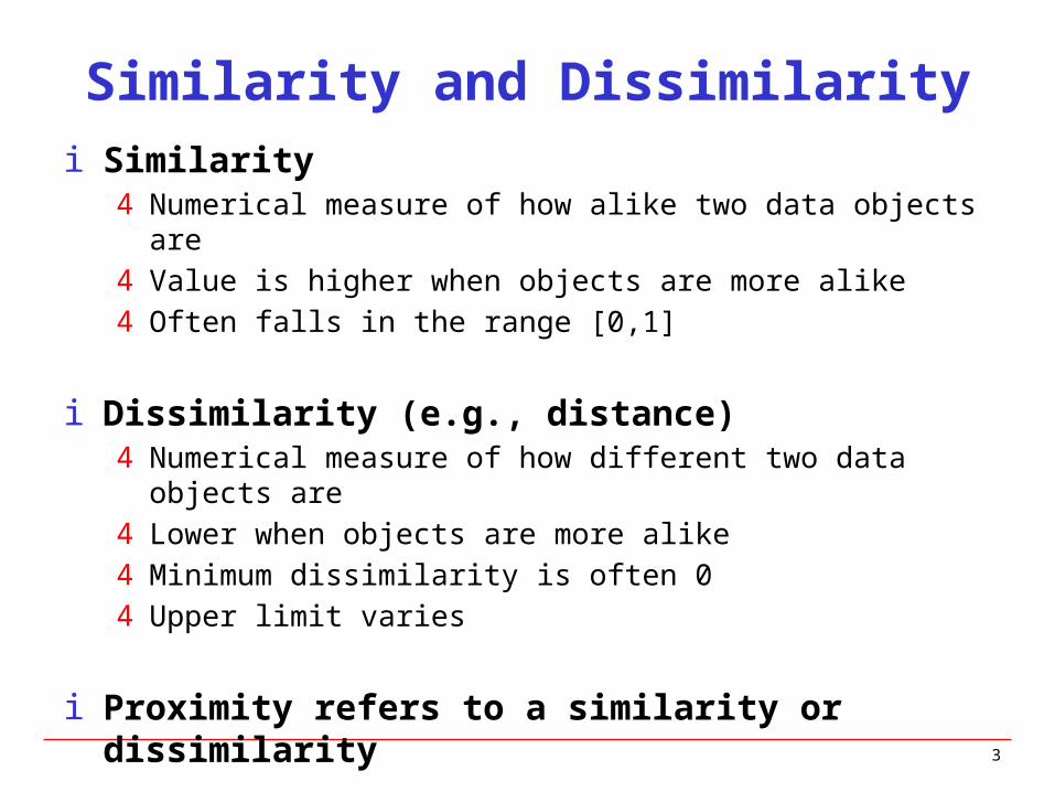
Similarity and Dissimilarityi Similarity
4 Numerical measure of how alike two data objects are4 Value is higher when objects are more alike4 Often falls in the range [0,1]
i Dissimilarity (e.g., distance)4 Numerical measure of how different two data objects are4 Lower when objects are more alike4 Minimum dissimilarity is often 04 Upper limit varies
i Proximity refers to a similarity or dissimilarity
3
4
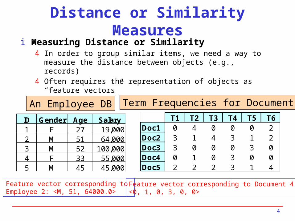
Distance or Similarity Measuresi Measuring Distance or Similarity
4 In order to group similar items, we need a way to measure the distance between objects (e.g., records)
4 Often requires the representation of objects as “feature vectors”
ID Gender Age Salary1 F 27 19,0002 M 51 64,0003 M 52 100,0004 F 33 55,0005 M 45 45,000
T1 T2 T3 T4 T5 T6Doc1 0 4 0 0 0 2Doc2 3 1 4 3 1 2Doc3 3 0 0 0 3 0Doc4 0 1 0 3 0 0Doc5 2 2 2 3 1 4
An Employee DB Term Frequencies for Documents
Feature vector corresponding to Employee 2: <M, 51, 64000.0>
Feature vector corresponding to Document 4: <0, 1, 0, 3, 0, 0>

5
Distance or Similarity Measures
i Representation of objects as vectors:4 Each data object (item) can be viewed as an n-dimensional vector, where
the dimensions are the attributes (features) in the data4 Example (employee DB): Emp. ID 2 = <M, 51, 64000>4 Example (Documents): DOC2 = <3, 1, 4, 3, 1, 2>4 The vector representation allows us to compute distance or similarity
between pairs of items using standard vector operations, e.g., h Cosine of the angle between vectorsh Manhattan distanceh Euclidean distanceh Hamming Distance
i Properties of Distance Measures:4 for all objects A and B, dist(A, B) ³ 0, and dist(A, B) = dist(B, A)4 for any object A, dist(A, A) = 04 dist(A, C) £ dist(A, B) + dist (B, C)
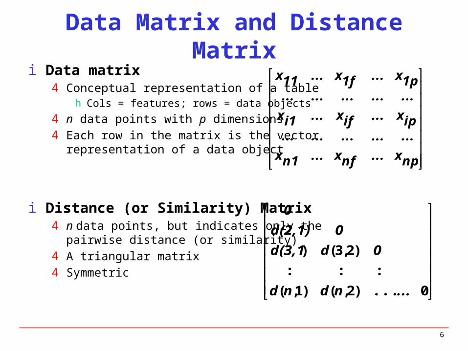
Data Matrix and Distance Matrixi Data matrix
4 Conceptual representation of a tableh Cols = features; rows = data objects
4 n data points with p dimensions4 Each row in the matrix is the vector
representation of a data object
i Distance (or Similarity) Matrix4 n data points, but indicates only the
pairwise distance (or similarity)4 A triangular matrix4 Symmetric
6
npx...nfx...n1x
...............ipx...ifx...i1x
...............1px...1fx...11x
0...)2,()1,(
:::
)2,3()
...ndnd
0dd(3,1
0d(2,1)
0

Proximity Measure for Nominal Attributes
i If object attributes are all nominal (categorical), then proximity measures are used to compare objects
i Can take 2 or more states, e.g., red, yellow, blue, green (generalization of a binary attribute)
i Method 1: Simple matching4 m: # of matches, p: total # of variables
i Method 2: Convert to Standard Spreadsheet format4 For each attribute A create M binary attribute for the M nominal states of A4 Then use standard vector-based similarity or distance metrics
7
pmpjid ),(
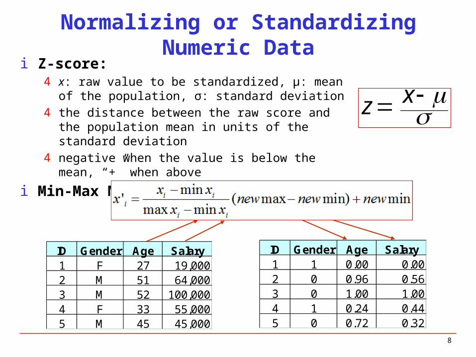
Normalizing or Standardizing Numeric Datai Z-score:
4 x: raw value to be standardized, μ: mean of the population, σ: standard deviation
4 the distance between the raw score and the population mean in units of the standard deviation
4 negative when the value is below the mean, “+” when above
i Min-Max Normalization
x z
8
ID Gender Age Salary1 F 27 19,0002 M 51 64,0003 M 52 100,0004 F 33 55,0005 M 45 45,000
ID Gender Age Salary1 1 0.00 0.002 0 0.96 0.563 0 1.00 1.004 1 0.24 0.445 0 0.72 0.32

9
Common Distance Measures for Numeric Data
i Consider two vectors4 Rows in the data matrix
i Common Distance Measures:
4 Manhattan distance:
4 Euclidean distance:
4 Distance can be defined as a dual of a similarity measure
( , ) 1 ( , )dist X Y sim X Y 2 2
( )( , )
i ii
i ii i
x ysim X Y
x y

10
Example: Data Matrix and Distance Matrixpoint attribute1 attribute2x1 1 2x2 3 5x3 2 0x4 4 5
Distance Matrix (Euclidean)x1 x2 x3 x4
x1 0
x2 3.61 0
x3 2.24 5.1 0
x4 4.24 1 5.39 0
Data Matrix
0 2 4
2
4
x1
x2
x3
x4
Distance Matrix (Manhattan)x1 x2 x3 x4
x1 0
x2 5 0
x3 3 6 0
x4 6 1 7 0

Distance on Numeric Data: Minkowski Distance
i Minkowski distance: A popular distance measure
4 where i = (xi1, xi2, …, xip) and j = (xj1, xj2, …, xjp) are two p-dimensional data objects, and h is the order (the distance so defined is also called L-h norm)
i Note that Euclidean and Manhattan distances are special cases4 h = 1: (L1 norm) Manhattan distance
4 h = 2: (L2 norm) Euclidean distance
11
)||...|||(|),( 22
22
2
11 pp jx
ix
jx
ix
jx
ixjid
||...||||),(2211 pp jxixjxixjxixjid
12
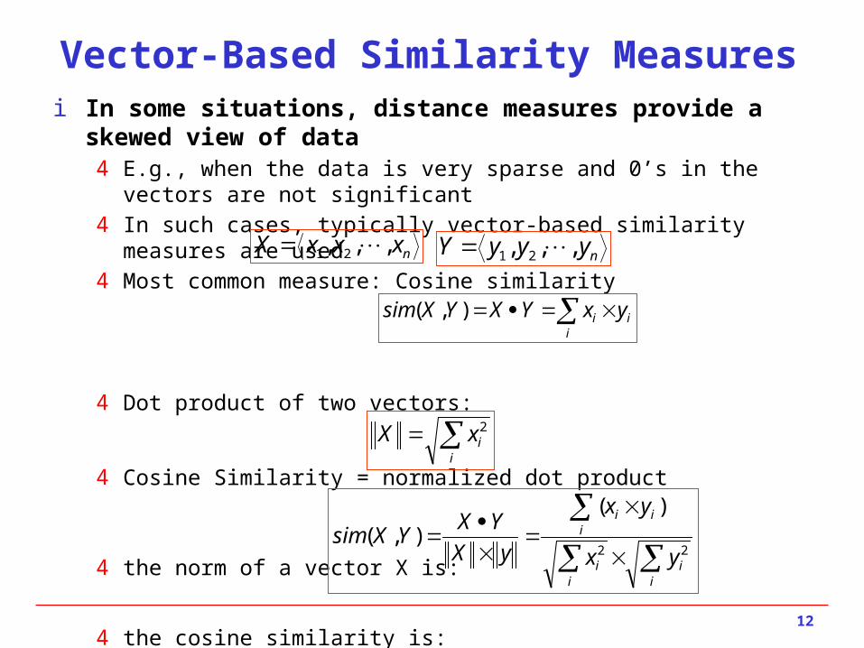
Vector-Based Similarity Measuresi In some situations, distance measures provide a skewed view of data
4 E.g., when the data is very sparse and 0’s in the vectors are not significant4 In such cases, typically vector-based similarity measures are used4 Most common measure: Cosine similarity
4 Dot product of two vectors:
4 Cosine Similarity = normalized dot product
4 the norm of a vector X is:
4 the cosine similarity is:
i
ixX 2
ii
ii
iii
yx
yx
yX
YXYXsim
22
)(),(
1 2, , , nX x x x 1 2, , , nY y y y
i
ii yxYXYXsim ),(
13
Vector-Based Similarity Measures
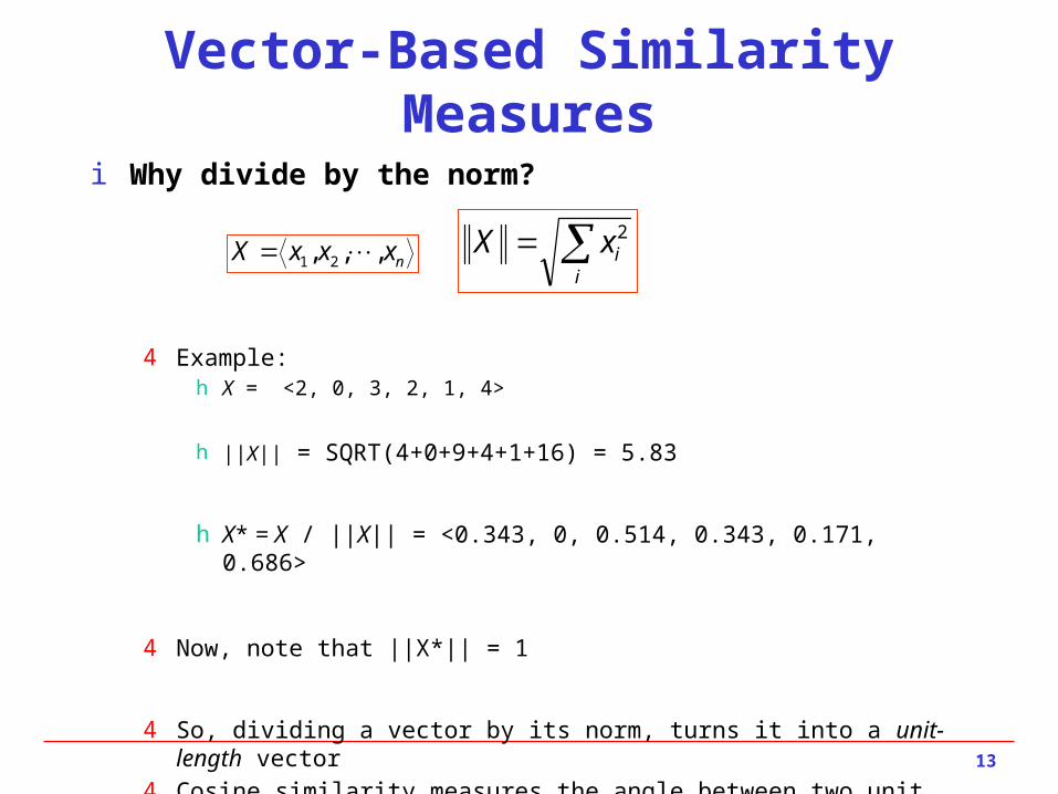
i Why divide by the norm?
4 Example:h X = <2, 0, 3, 2, 1, 4>
h ||X|| = SQRT(4+0+9+4+1+16) = 5.83
h X* = X / ||X|| = <0.343, 0, 0.514, 0.343, 0.171, 0.686>
4 Now, note that ||X*|| = 1
4 So, dividing a vector by its norm, turns it into a unit-length vector4 Cosine similarity measures the angle between two unit length vectors (i.e., the
magnitude of the vectors are ignored).
1 2, , , nX x x x i
ixX 2
14
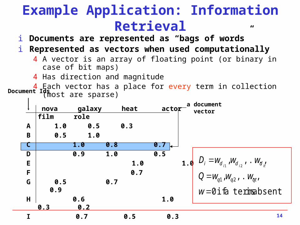
Example Application: Information Retrievali Documents are represented as “bags of words”i Represented as vectors when used computationally
4 A vector is an array of floating point (or binary in case of bit maps)4 Has direction and magnitude4 Each vector has a place for every term in collection (most are sparse)
nova galaxy heat actor film role
A 1.0 0.5 0.3
B 0.5 1.0
C 1.0 0.8 0.7
D 0.9 1.0 0.5
E 1.0 1.0
F 0.7
G 0.5 0.7 0.9
H 0.6 1.0 0.3 0.2
I 0.7 0.5 0.3
Document Ids
a documentvector
absent is terma if 0
,...,,
,...,,
21
21
w
wwwQ
wwwD
qtqq
dddi itii

Documents & Query in n-dimensional Space
15
i Documents are represented as vectors in the term space4 Typically values in each dimension correspond to the frequency of the
corresponding term in the document
i Queries represented as vectors in the same vector-spacei Cosine similarity between the query and documents is often used
to rank retrieved documents
16
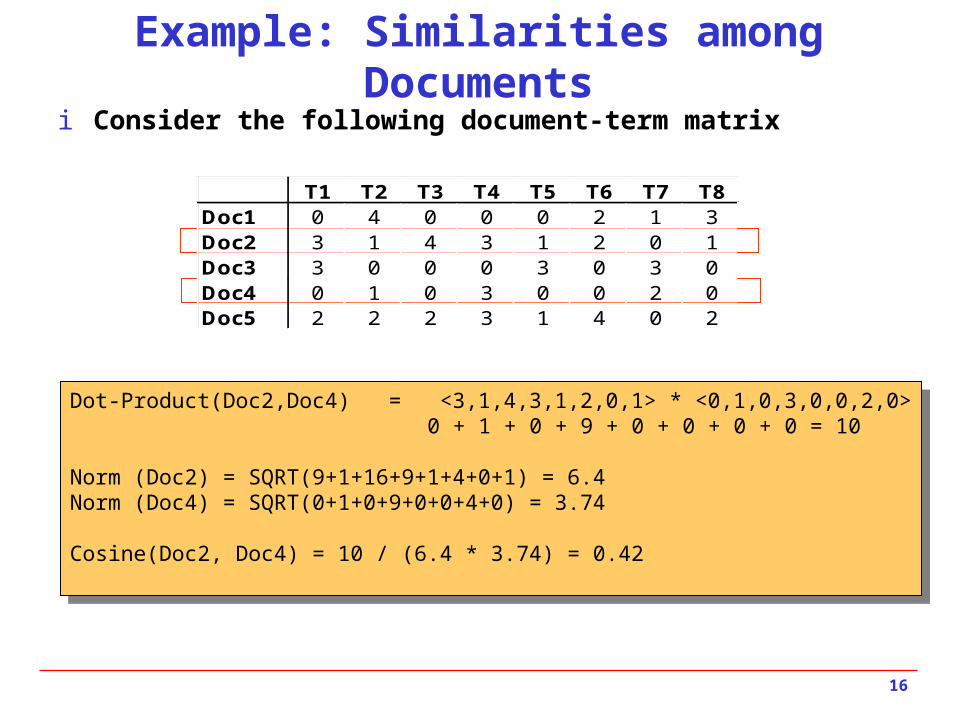
Example: Similarities among Documentsi Consider the following document-term matrix
T1 T2 T3 T4 T5 T6 T7 T8Doc1 0 4 0 0 0 2 1 3Doc2 3 1 4 3 1 2 0 1Doc3 3 0 0 0 3 0 3 0Doc4 0 1 0 3 0 0 2 0Doc5 2 2 2 3 1 4 0 2
Dot-Product(Doc2,Doc4) = <3,1,4,3,1,2,0,1> * <0,1,0,3,0,0,2,0> 0 + 1 + 0 + 9 + 0 + 0 + 0 + 0 = 10
Norm (Doc2) = SQRT(9+1+16+9+1+4+0+1) = 6.4Norm (Doc4) = SQRT(0+1+0+9+0+0+4+0) = 3.74
Cosine(Doc2, Doc4) = 10 / (6.4 * 3.74) = 0.42
Dot-Product(Doc2,Doc4) = <3,1,4,3,1,2,0,1> * <0,1,0,3,0,0,2,0> 0 + 1 + 0 + 9 + 0 + 0 + 0 + 0 = 10
Norm (Doc2) = SQRT(9+1+16+9+1+4+0+1) = 6.4Norm (Doc4) = SQRT(0+1+0+9+0+0+4+0) = 3.74
Cosine(Doc2, Doc4) = 10 / (6.4 * 3.74) = 0.42

Correlation as Similarity
i In cases where there could be high mean variance across data objects (e.g., movie ratings), Pearson Correlation coefficient is the best option
i Pearson Correlation
i Often used in recommender systems based on Collaborative Filtering
17
18
Distance-Based Classificationi Basic Idea: classify new instances based on their similarity to or
distance from instances we have seen before4 Sometimes called “instance-based learning”
i Basic Idea:4 Save all previously encountered instances4 Given a new instance, find those instances that are most similar to the new one4 Assign new instance to the same class as these “nearest neighbors”
i “Lazy” Classifiers4 The approach defers all of the real work until new instance is obtained; no
attempt is made to learn a generalized model from the training set4 Less data preprocessing and model evaluation, but more work has to be done at
classification time

Nearest Neighbor Classifiersi Basic idea:
4 If it walks like a duck, quacks like a duck, then it’s probably a duck
19
Training Records
Test Record
Compute Distance
Choose k of the “nearest” records

K-Nearest-Neighbor Strategyi Given object x, find the k most similar objects to x
4 The k nearest neighbors4 Variety of distance or similarity measures can be used to identify and rank
neighbors4 Note that this requires comparison between x and all objects in the database
i Classification:4 Find the class label for each of the k neighbor4 Use a voting or weighted voting approach to determine the majority class
among the neighbors (a combination function)h Weighted voting means the closest neighbors count more
4 Assign the majority class label to x
i Prediction:4 Identify the value of the target attribute for the k neighbors4 Return the weighted average as the predicted value of the target attribute for x
20

21
Combination Functions
i Once the Nearest Neighbors are identified, the “votes” of these neighbors must be combined to generate a prediction
i Voting: the “democracy” approach4 poll the neighbors for the answer and use the majority vote4 the number of neighbors (k) is often taken to be odd in order to avoid ties
h works when the number of classes is twoh if there are more than two classes, take k to be the number of classes plus 1
i Impact of k on predictions4 in general different values of k affect the outcome of classification4 we can associate a confidence level with predictions (this can be the % of
neighbors that are in agreement)4 problem is that no single category may get a majority vote4 if there is strong variations in results for different choices of k, this an
indication that the training set is not large enough
22
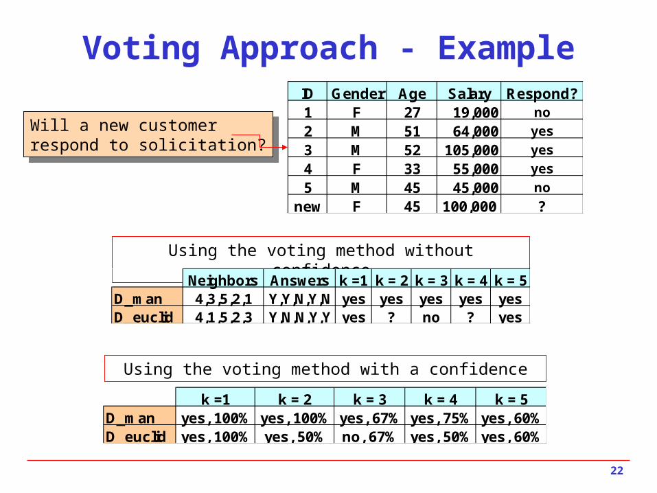
Voting Approach - ExampleID Gender Age Salary Respond?1 F 27 19,000 no
2 M 51 64,000 yes
3 M 52 105,000 yes
4 F 33 55,000 yes
5 M 45 45,000 no
new F 45 100,000 ?
Neighbors Answers k =1 k = 2 k = 3 k = 4 k = 5D_man 4,3,5,2,1 Y,Y,N,Y,N yes yes yes yes yesD_euclid 4,1,5,2,3 Y,N,N,Y,Y yes ? no ? yes
k =1 k = 2 k = 3 k = 4 k = 5D_man yes, 100% yes, 100% yes, 67% yes, 75% yes, 60%D_euclid yes, 100% yes, 50% no, 67% yes, 50% yes, 60%
Will a new customerrespond to solicitation?
Will a new customerrespond to solicitation?
Using the voting method without confidence
Using the voting method with a confidence
23
Combination Functionsi Weighted Voting: not so “democratic”
4 similar to voting, but the vote some neighbors counts more4 “shareholder democracy?”4 question is which neighbor’s vote counts more?
i How can weights be obtained?4 Distance-based
h closer neighbors get higher weightsh “value” of the vote is the inverse of the distance (may need to add a small constant)h the weighted sum for each class gives the combined score for that classh to compute confidence, need to take weighted average
4 Heuristich weight for each neighbor is based on domain-specific characteristics of that neighbor
i Advantage of weighted voting4 introduces enough variation to prevent ties in most cases4 helps distinguish between competing neighbors
24
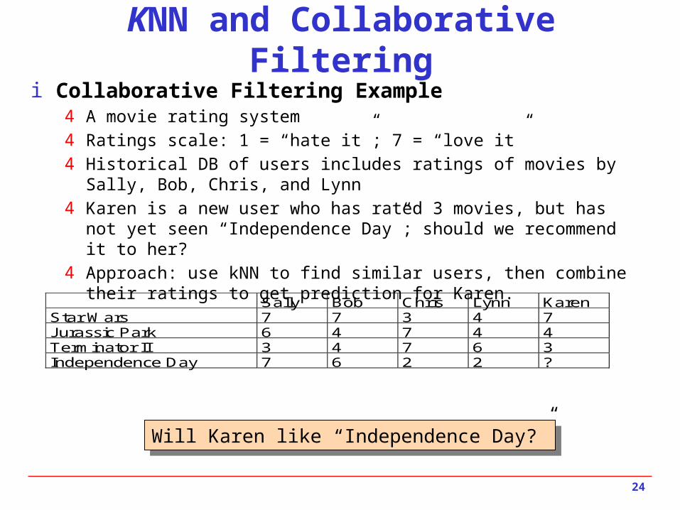
KNN and Collaborative Filteringi Collaborative Filtering Example
4 A movie rating system4 Ratings scale: 1 = “hate it”; 7 = “love it”4 Historical DB of users includes ratings of movies by Sally, Bob, Chris, and Lynn4 Karen is a new user who has rated 3 movies, but has not yet seen “Independence
Day”; should we recommend it to her?4 Approach: use kNN to find similar users, then combine their ratings to get
prediction for Karen.
Sally Bob Chris Lynn Karen Star Wars 7 7 3 4 7 Jurassic Park 6 4 7 4 4 Terminator II 3 4 7 6 3 Independence Day 7 6 2 2 ?
Will Karen like “Independence Day?”Will Karen like “Independence Day?”

25
Collaborative Filtering(k Nearest Neighbor Example)
Star Wars Jurassic Park Terminator 2 Indep. Day Average Cosine Distance Euclid PearsonSally 7 6 3 7 5.33 0.983 2 2.00 0.85Bob 7 4 4 6 5.00 0.995 1 1.00 0.97Chris 3 7 7 2 5.67 0.787 11 6.40 -0.97Lynn 4 4 6 2 4.67 0.874 6 4.24 -0.69
Karen 7 4 3 ? 4.67 1.000 0 0.00 1.00
K Pearson1 62 6.53 5
Example computation:
Pearson(Sally, Karen) = ( (7-5.33)*(7-4.67) + (6-5.33)*(4-4.67) + (3-5.33)*(3-4.67) ) / SQRT( ((7-5.33)2 +(6-5.33)2 +(3-5.33)2) * ((7- 4.67)2 +(4- 4.67)2 +(3- 4.67)2)) = 0.85
K is the number of nearestneighbors used in to find theaverage predicted ratings ofKaren on Indep. Day.
K is the number of nearestneighbors used in to find theaverage predicted ratings ofKaren on Indep. Day.
Prediction
Distance and Similarity Measures
Bamshad Mobasher
DePaul University