Embed Size (px)
Citation preview
DISSERTATION
Titel der Dissertation
Sobolev metrics on shape space of surfaces
Verfasser
Philipp Harms
angestrebter akademischer Grad
Doktor der Naturwissenschaften (Dr. rer. nat.)
Wien, Oktober 2010
Studienkennzahl lt. Studienblatt: A 091 405Dissertationsgebiet lt. Studienblatt: MathematikBetreuer: Ao. Univ.-Prof. Dr. Peter W. Michor

ii
iii
In nova fert animus mutatas dicere formascorpora; di, coeptis (nam vos mutastis et illas)adspirate meis primaque ab origine mundiad mea perpetuum deducite tempora carmen!
∗The persistence of memory by Salvador Dali. Picture taken from http://en.wikipedia.
org/wiki/File:The_Persistence_of_Memory.jpg, November 2010.†Proemium of Ovid’s metamorphoses.

iv

v
Abstract. Many procedures in science, engineering and medicine produce datain the form of geometric shapes. Mathematically, a shape can be modeled asan un-parameterized immersed sub-manifold, which is the notion of shape usedhere. Endowing shape space with a Riemannian metric opens up the world ofRiemannian differential geometry with geodesics, gradient flows and curvature.Unfortunately, the simplest such metric induces vanishing path-length distanceon shape space. This discovery by Michor and Mumford was the starting pointto a quest for stronger, meaningful metrics that should be able to distinguishsalient features of the shapes. Sobolev metrics are a very promising approachto that. They come in two flavors: Outer metrics which are induced frommetrics on the diffeomorphism group of ambient space, and inner metrics whichare defined intrinsically to the shape. In this work, Sobolev inner metrics aredeveloped and treated in a very general setting. There are no restrictions on thedimension of the immersed space or of the ambient space, and ambient spaceis not required to be flat. It is shown that the path-length distance induced bySobolev inner metrics does not vanish. The geodesic equation and the conservedquantities arising from the symmetries are calculated, and well-posedness of thegeodesic equation is proven. Finally examples of numerical solutions to thegeodesic equation are presented.

vi
vii
Acknowledgment. I am very thankful for the support I have received fromso many sides during my time as a Ph.D. student. First of all I want to thankmy very dear advisor Peter W. Michor. I would also like to thank Alain Troue,Bianca Falcidieno, Silvia Biasotti, Darryl Holm and Andrea Mennucci who haveinvited me to research visits at their institutes; David Mumford, Stefan Haller,Johannes Wallner and Hermann Schichl who have helped me in mathematicalquestions; Peter Gruber and Josef Teichmann for their ongoing caring interest inmy mathematical and personal welfare; Andreas Kriegl, Dietrich Burde, ArminRainer and Andreas Nemeth for their merry company at so many meals andcoffee breaks; Martin Bauer for bearing with me during all those years as friendsand colleagues; my friends, siblings and parents for being such good friends,siblings and parents!

viii

Contents
Preface v
Abstract . . . . . . . . . . . . . . . . . . . . . . . . . . . . . . . . . . . v
Acknowledgment . . . . . . . . . . . . . . . . . . . . . . . . . . . . . . vii
Contents . . . . . . . . . . . . . . . . . . . . . . . . . . . . . . . . . . . vii
1 Introduction 1
1.1 The Riemannian setting for shape analysis . . . . . . . . . . . . . 1
1.2 Related work . . . . . . . . . . . . . . . . . . . . . . . . . . . . . 2
1.3 Inner versus outer metrics . . . . . . . . . . . . . . . . . . . . . . 2
1.4 Where this work comes from . . . . . . . . . . . . . . . . . . . . 4
1.5 Content of this work . . . . . . . . . . . . . . . . . . . . . . . . . 5
1.6 Contributions of this work. . . . . . . . . . . . . . . . . . . . . . 6
2 Notation 7
2.1 Basic assumptions and conventions . . . . . . . . . . . . . . . . . 7
2.2 Tensor bundles and tensor fields . . . . . . . . . . . . . . . . . . 8
2.3 Metric on tensor spaces . . . . . . . . . . . . . . . . . . . . . . . 8
2.4 Traces . . . . . . . . . . . . . . . . . . . . . . . . . . . . . . . . . 9
2.5 Volume density . . . . . . . . . . . . . . . . . . . . . . . . . . . . 9
2.6 Metric on tensor fields . . . . . . . . . . . . . . . . . . . . . . . . 9
2.7 Covariant derivative . . . . . . . . . . . . . . . . . . . . . . . . . 10
2.8 Swapping covariant derivatives . . . . . . . . . . . . . . . . . . . 11
2.9 Second and higher covariant derivatives . . . . . . . . . . . . . . 11
2.10 Adjoint of the covariant derivative . . . . . . . . . . . . . . . . . 11
ix

x CONTENTS
2.11 Laplacian . . . . . . . . . . . . . . . . . . . . . . . . . . . . . . . 12
2.12 Normal bundle . . . . . . . . . . . . . . . . . . . . . . . . . . . . 12
2.13 Second fundamental form and Weingarten mapping . . . . . . . . 13
3 Shape space 15
3.1 Convenient calculus . . . . . . . . . . . . . . . . . . . . . . . . . 15
3.2 Manifolds of immersions and embeddings . . . . . . . . . . . . . 17
3.3 Bundles of multilinear maps over immersions . . . . . . . . . . . 18
3.4 Diffeomorphism group . . . . . . . . . . . . . . . . . . . . . . . . 19
3.5 Riemannian metrics on immersions . . . . . . . . . . . . . . . . . 19
3.6 Covariant derivative ∇g on immersions . . . . . . . . . . . . . . . 20
3.7 Metric gradients . . . . . . . . . . . . . . . . . . . . . . . . . . . 20
3.8 Geodesic equation on immersions . . . . . . . . . . . . . . . . . . 21
3.9 Geodesic equation on immersions . . . . . . . . . . . . . . . . . . 22
3.10 Conserved momenta . . . . . . . . . . . . . . . . . . . . . . . . . 23
3.11 Shape space . . . . . . . . . . . . . . . . . . . . . . . . . . . . . . 25
3.12 Riemannian submersions and geodesics . . . . . . . . . . . . . . . 25
3.13 Riemannian metrics on shape space . . . . . . . . . . . . . . . . . 26
3.14 Geodesic equation on shape space . . . . . . . . . . . . . . . . . . 26
3.15 Geodesic equation on shape space . . . . . . . . . . . . . . . . . . 28
3.16 Inner versus outer metrics . . . . . . . . . . . . . . . . . . . . . . 29
4 Variational formulas 31
4.1 Paths of immersions . . . . . . . . . . . . . . . . . . . . . . . . . 31
4.2 Directional derivatives of functions . . . . . . . . . . . . . . . . . 32
4.3 Setting for first variations . . . . . . . . . . . . . . . . . . . . . . 32
4.4 Variation of equivariant tensor fields . . . . . . . . . . . . . . . . 32
4.5 Variation of the metric . . . . . . . . . . . . . . . . . . . . . . . . 33
4.6 Variation of the inverse of the metric . . . . . . . . . . . . . . . . 33
4.7 Variation of the volume density . . . . . . . . . . . . . . . . . . . 34
4.8 Variation of the covariant derivative . . . . . . . . . . . . . . . . 35
4.9 Variation of the Laplacian . . . . . . . . . . . . . . . . . . . . . . 35
CONTENTS xi
5 Sobolev-type metrics 39
5.1 Invariance of P under reparametrizations . . . . . . . . . . . . . 39
5.2 The adjoint of ∇P . . . . . . . . . . . . . . . . . . . . . . . . . . 40
5.3 Metric gradients . . . . . . . . . . . . . . . . . . . . . . . . . . . 41
5.4 Geodesic equation . . . . . . . . . . . . . . . . . . . . . . . . . . 42
5.5 Geodesic equation . . . . . . . . . . . . . . . . . . . . . . . . . . 43
5.6 Well-posedness of the geodesic equation . . . . . . . . . . . . . . 43
5.7 Momentum mappings . . . . . . . . . . . . . . . . . . . . . . . . 47
5.8 Horizontal bundle . . . . . . . . . . . . . . . . . . . . . . . . . . . 48
5.9 Horizontal curves . . . . . . . . . . . . . . . . . . . . . . . . . . . 49
5.10 Geodesic equation . . . . . . . . . . . . . . . . . . . . . . . . . . 50
5.11 Geodesic equation . . . . . . . . . . . . . . . . . . . . . . . . . . 50
6 Geodesic distance on shape space 53
6.1 Geodesic distance on shape space . . . . . . . . . . . . . . . . . . 53
6.2 Vanishing geodesic distance . . . . . . . . . . . . . . . . . . . . . 54
6.3 Area swept out . . . . . . . . . . . . . . . . . . . . . . . . . . . . 57
6.4 First area swept out bound . . . . . . . . . . . . . . . . . . . . . 57
6.5 Lipschitz continuity of√
Vol . . . . . . . . . . . . . . . . . . . . . 58
6.6 Non-vanishing geodesic distance . . . . . . . . . . . . . . . . . . . 58
7 Sobolev metrics induced by the Laplacian 61
7.1 Other choices for P . . . . . . . . . . . . . . . . . . . . . . . . . . 61
7.2 Adjoint of ∇P . . . . . . . . . . . . . . . . . . . . . . . . . . . . 62
7.3 Geodesic equations and conserved momentum . . . . . . . . . . . 65
8 Surfaces in n-space 67
8.1 Geodesic equation . . . . . . . . . . . . . . . . . . . . . . . . . . 67
8.2 Additional conserved momenta . . . . . . . . . . . . . . . . . . . 69
8.3 Frechet distance and Finsler metric . . . . . . . . . . . . . . . . . 69
8.4 Sobolev versus Frechet distance . . . . . . . . . . . . . . . . . . . 70
8.5 Concentric spheres . . . . . . . . . . . . . . . . . . . . . . . . . . 71

xii CONTENTS
9 Diffeomorphism groups 73
10 Numerical results 75
Appendix 81
Bibliography . . . . . . . . . . . . . . . . . . . . . . . . . . . . . . . . 81
Zusammenfassung . . . . . . . . . . . . . . . . . . . . . . . . . . . . . 85
Curriculum Vitae . . . . . . . . . . . . . . . . . . . . . . . . . . . . . . 87

Chapter 1
Introduction
1.1 The Riemannian setting for shape analysis
From very early on, shapes spaces have been analyzed in a Riemannian setting.This is also the setting that has been adopted in this work. The Riemanniansetting is well-suited to shape analysis for several reasons.
• It formalizes an intuitive notion of similarity of shapes: Shapes that differonly by a small deformation are similar to each other. To compare shapes,it is thus necessary to measure deformations. This is exactly what isaccomplished by a Riemannian metric. A Riemannian metric measurescontinuous deformations of shapes, that is, paths in shape space.
• Riemannian metrics on shape space have been used successfully in com-puter vision for a long time, often without any mention of the underlyingmetric. Gradient flows for shape smoothing are an example. An under-lying metric is needed for the definition of a gradient. Often, the metricthat has been used implicitly was the L2-metric that has however turnedout to be too weak.
• The exponential map that is induced by a Riemannian metric permits tolinearize shape space: When shapes are represented as initial velocities ofgeodesics connecting them to a fixed reference shape, one effectively worksin the linear tangent space over the reference shape. Curvature will playan essential role in quantifying the deviation of curved shape space fromits linearized approximation.
• The linearization of shape space by the exponential map allows to dostatistics on shape space.
A disadvantage of the Riemannian approach is that shapes can be comparedwith each other only when there is a deformation between them.
1
2 CHAPTER 1. INTRODUCTION
1.2 Related work
In mathematics and computer vision, shapes have been represented in manyways. Point clouds, meshes, level-sets, graphs of a function, currents and mea-sures are but some of the possibilities. Furthermore, the resulting shape spaceshave been endowed with many different metrics. Approaches found in the liter-ature include:
• Inner metrics on shape space of unparametrized immersions. These met-rics are induced from metrics on parametrized immersions. Since this isthe approach studied in this work, more references will be given later.
• Outer metrics on various shape spaces (images, embedded surfaces, land-marks, measures and currents) that the diffeomorphism group of ambientspace is acting on. See for example [6, 11, 39, 40, 16, 33, 26, 24].
• Metamorphosis metrics. See for example [47, 25].
• The Wasserstein metric or Monge-Kantorovic metric on shape space ofprobability measures. See for example [2, 3, 13, 12].
• The Weil-Peterson metric on shape space of planar curves. See for example[42, 43, 30].
• Current metrics. See for example [48, 19, 20].
More references can be found in the review papers [1, 4, 14, 31, 41, 49].
1.3 Inner versus outer metrics
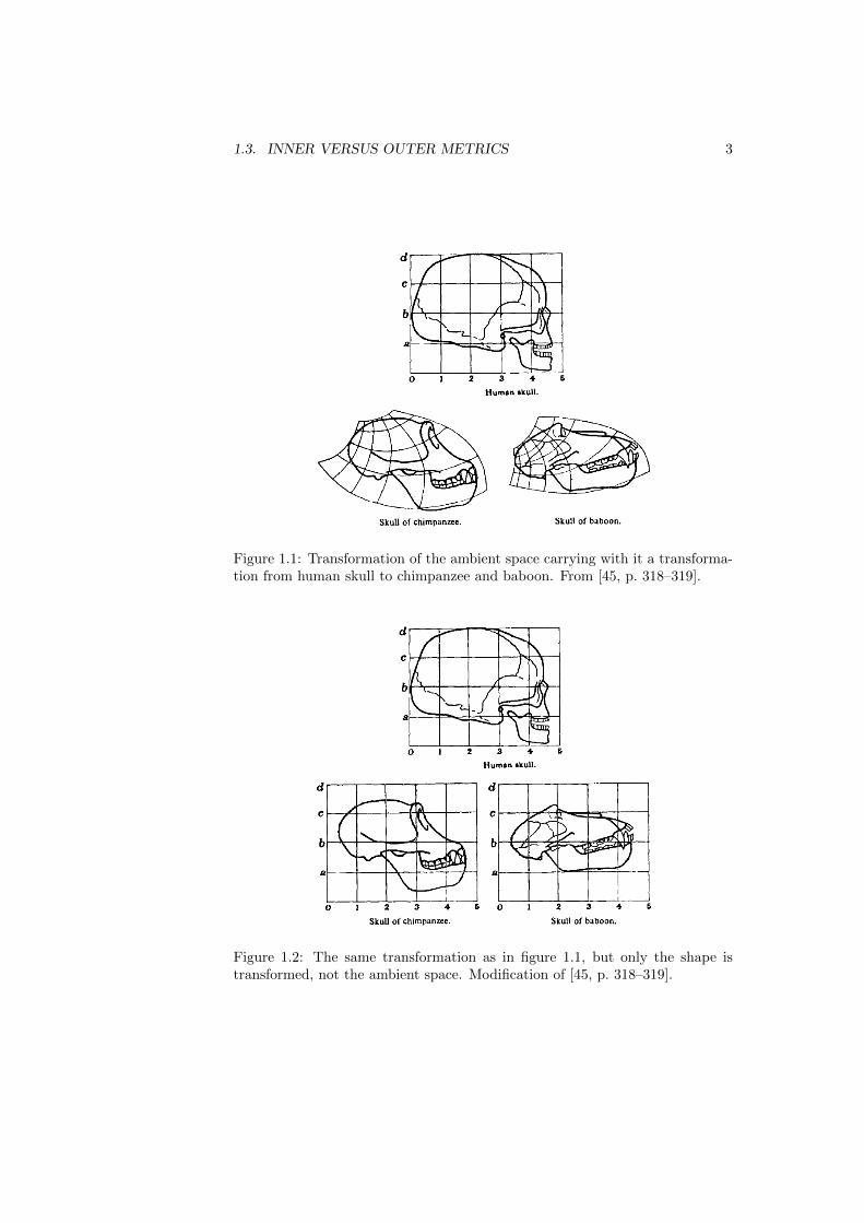
Outer metrics measure how much ambient space has to be deformed in order toyield the desired deformation of the shape. This concept has been introduced bythe Scottish biologist, mathematician and classics scholar d’Arcy Thompson in1942, already. As Thompson declared in the epilogue of his book “On Growthand Form” [45], his aim was to show that “a certain mathematical aspect ofmorphology is essential to (the) proper study of Growth and Form”. In thechapter “On the comparison of related forms” of this book, Thompson picturestransformations of the ambient space by a Cartesian grid. A transformation ofthe ambient space and the grid then results in a deformation of the embeddedshape, too. An example is given in figure 1.1.
Thompson’s notion of shape transformation and the concept of outer metricsis fundamentally different from the notion of shape transformation that underliesthis work. In this work, so called inner metrics are treated. Inner metricsmeasure how much the shape itself is deformed. A deformation of the shapedoes not carry with it a deformation of the ambient space. The ambient spaceis fixed, and the shape moves within it. This is illustrated in figure 1.2.
Riemannian metrics on shape space measure infinitesimal deformations. Aninfinitesimal deformation of ambient space is a vector field on ambient space and
1.3. INNER VERSUS OUTER METRICS 3
Figure 1.1: Transformation of the ambient space carrying with it a transforma-tion from human skull to chimpanzee and baboon. From [45, p. 318–319].
Figure 1.2: The same transformation as in figure 1.1, but only the shape istransformed, not the ambient space. Modification of [45, p. 318–319].

4 CHAPTER 1. INTRODUCTION
could be pictured as a small arrow attached to every point in ambient space.This is the kind of deformation that is measured by outer metrics. In contrast tothis, an infinitesimal deformation of the shape itself is a (normal or horizontal)vector field along the shape. It could be pictured as a small arrow attached toevery point of the shape. Figure 1.3 illustrates the two kinds of deformation.
Figure 1.3: Infinitesimal transformation of ambient space (left) as measured byan outer metric and infinitesimal transformation of the shape itself (right) asmeasured by an inner metric.
The deformations that are measured by inner metrics have much smaller(lower dimensional) support than those measured by outer metrics. This isan advantage in numerics. A disadvantage is that the differential operatorgoverning an inner metric usually depends on the shape, which is not the casefor outer metrics.
Section 3.16 explains how the difference between inner and outer metricsbecomes manifest in the mathematical theory. Sections 3.3 and 3.13 explain inmathematical terms what an infinitesimal deformation of a shape is.
1.4 Where this work comes from
This work continues the study of inner metrics on shape space of unparametrizedimmersions of a fixed manifold M into a Riemannian manifold N . M fixes thetopology of the shapes. N is the ambient space, and it is endowed with a fixedmetric. For example, M could be a simple geometric object like a sphere, andN could be some Rn.
It came as a big surprise when Michor and Mumford found out in [38, 37] thatthe simplest and most natural Riemannian metric on this shape space (the L2-metric) induces vanishing geodesic distance on shape space. More precisely theresult is that any two shapes can be deformed into each other by a deformationthat is arbitrarily small when measured with respect to this metric. The resultalso holds for L2-metrics on diffeomorphism groups and for outer L2-metrics onshape space. The discovery of this degeneracy was the starting point to a questfor stronger metrics. These metrics should be able to distinguish salient featuresof the shapes. The meaning of salient of course depends on the application.
One approach to strengthen the L2 inner metric is by weighting it by a

1.5. CONTENT OF THIS WORK 5
function depending on the mean curvature and/or the volume [38, 37, 7, 9, 10].Such metrics have been called almost local metrics.
Another approach, and the approach taken in this work, is to incorporatederivatives of the deformation vector fields in the definition of the metric. Thisyields Sobolev inner metrics on shape space. Sobolev inner metrics have firstbeen defined on shape space of planar curves [39, 51, 52, 46, 32]. In this workand in [8], these metrics are generalized to higher dimensional shape spaces andto a possibly curved ambient space.
Some parts of this work have been written in collaboration with MartinBauer and can also be found in his thesis [10]. This concerns mainly sections 2,3 and 4 covering a lot of background material.
1.5 Content of this work
This work progresses from a very general setting to a specific one in three steps.In the beginning, a framework for general inner metrics is developed. Then thegeneral concepts carry over to more and more specific inner metrics.
• First, shape space is endowed with a general inner metric, i.e with ametric that is induced from a metric on the space of immersions, butthat is unspecified otherwise. It is shown how various versions of thegeodesic equation can be expressed using gradients of the metric withrespect to itself and how conserved quantities arise from symmetries. (Thisis section 3.)
• Then it is assumed that the inner metric is defined via an elliptic pseudo-differential operator. Such a metric will be called a Sobolev-type metric.The geodesic equation is formulated in terms of the operator, and existenceof horizontal paths of immersions within each equivalence class of pathsis proven. (This is section 5.) Then estimates on the path-length distanceare derived. Most importantly it is shown that when the operator involveshigh enough powers of the Laplacian, then the metric does not have thedegeneracy of the L2-metric. (This is section 6.)
• Motivated by the previous results it is assumed that the elliptic pseudo-differential operator is given by the Laplacian and powers of it. Again, thegeodesic equation is derived. The formulas that are obtained are ready tobe implemented numerically. (This is section 7.)
The remaining sections cover the following material:
• Section 2 treats some differential geometry of surfaces that is neededthroughout this work. It is also a good reference for the notation thatis used. The biggest emphasis is on a rigorous treatment of the covariantderivative. Some material like the adjoint covariant derivative is not foundin standard text books.

6 CHAPTER 1. INTRODUCTION
• Section 4 contains formulas for the variation of the metric, volume form,covariant derivative and Laplacian with respect to the immersion inducingthem. These formulas are used extensively later.
• Section 8 covers the special case of flat ambient space. The geodesic equa-tion is simplified and conserved momenta for the Euclidean motion groupare calculated. Sobolev-type metrics are compared to the Frechet metricwhich is available in flat ambient space.
• Section 9 treats diffeomorphism groups of compact manifolds as a specialcase of the theory that has been developed so far.
• In section 10 it is shown in some examples that the geodesic equation onshape space can be solved numerically.
1.6 Contributions of this work.
• This work is the first to treat Sobolev inner metrics on spaces of immersedsurfaces and on higher dimensional shape spaces.
• It contains the first description of how the geodesic equation can be for-mulated in terms of gradients of the metric with respect to itself when theambient space is not flat. To achieve this, a covariant derivative on somebundles over immersions is defined. This covariant derivative is inducedfrom the Levi-Civita covariant derivative on ambient space.
• The geodesic equation is formulated in terms of this covariant derivative.Well-posedness of the geodesic equation is shown under some regularityassumptions that are verified for Sobolev metrics. Well-posedness alsofollows for the geodesic equation on diffeomorphism groups, where thisresult has not yet been obtained in that full generality.
• To derive the geodesic equation, a variational formula for the Laplacianoperator is developed. The variation is taken with respect to the metric onthe manifold where the Laplacian is defined. This metric in turn dependson the immersion inducing it.
• It is shown that Sobolev inner metrics separate points in shape space whenthe order of the differential operator governing the metric is high enough.(The metric needs to be as least as strong as the H1-metric.) Thus Sobolevinner metrics overcome the degeneracy of the L2-metric.
• The path-length distance of Sobolev inner metrics is compared to theFrechet distance. It would be desirable to bound Fechet distance by someSobolev distance. This however remains an open problem.
• Finally it is demonstrated in some examples that the geodesic equation forthe H1-metric on shape space of surfaces in R3 can be solved numerically.
Chapter 2
Differential geometry ofsurfaces and notation
In this section the differential geometric tools that are needed to deal withimmersed surfaces are presented and developed. The most important point is arigorous treatment of the covariant derivative and related concepts.
The notation of [36] is used. Some of the definitions can also be found in[27]. A similar exposition in the same notation is [7, 8]. This section has beenwritten in collaboration with Martin Bauer and is the same as section 1.1 of hisPh.D. thesis [10], up to slight modifications.
2.1 Basic assumptions and conventions
Assumption. It is always assumed that M and N are connected manifolds offinite dimensions m and n, respectively. Furthermore it is assumed that M iscompact, and that N is endowed with a Riemannian metric g.
In this work, immersions of M into N will be treated, i.e. smooth func-tions M → N with injective tangent mapping at every point. The set of allsuch immersions will be denoted by Imm(M,N). It is clear that only the casedim(M) ≤ dim(N) is of interest since otherwise Imm(M,N) would be empty.
Immersions or paths of immersions are usually denoted by f . Vector fieldson Imm(M,N) or vector fields along f will be called h, k,m, for example. Sub-scripts like ft = ∂tf = ∂f/∂t denote differentiation with respect to the indicatedvariable, but subscripts are also used to indicate the foot point of a tensor field.
7

8 CHAPTER 2. NOTATION
2.2 Tensor bundles and tensor fields
The tensor bundles
T rsM
T rsM ⊗ f∗TN
M M
will be used. Here T rsM denotes the bundle of ( rs )-tensors on M , i.e.
T rsM =
r⊗TM ⊗
s⊗T ∗M,
and f∗TN is the pullback of the bundle TN via f , see [36, section 17.5]. Atensor field is a section of a tensor bundle. Generally, when E is a bundle, thespace of its sections will be denoted by Γ(E).
To clarify the notation that will be used later, some examples of tensor bun-dles and tensor fields are given now. SkT ∗M = Lksym(TM ;R) and ΛkT ∗M =
Lkalt(TM ;R) are the bundles of symmetric and alternating ( 0k )-tensors, respec-
tively. Ωk(M) = Γ(ΛkT ∗M) is the space of differential forms, X(M) = Γ(TM)is the space of vector fields, and
Γ(f∗TN) ∼=h ∈ C∞(M,TN) : πN h = f
is the space of vector fields along f .
2.3 Metric on tensor spaces
Let g ∈ Γ(S2>0T
∗N) denote a fixed Riemannian metric on N . The metricinduced on M by f ∈ Imm(M,N) is the pullback metric
g = f∗g ∈ Γ(S2>0T
∗M), g(X,Y ) = (f∗g)(X,Y ) = g(Tf.X, Tf.Y ),
where X,Y are vector fields on M . The dependence of g on the immersion fshould be kept in mind. Let
[ = g : TM → T ∗M and ] = g−1 : T ∗M → TM.
g can be extended to the cotangent bundle T ∗M = T 01M by setting
g−1(α, β) = g01(α, β) = α(β])
for α, β ∈ T ∗M . The product metric
grs =
r⊗g ⊗
s⊗g−1
extends g to all tensor spaces T rsM , and grs⊗g yields a metric on T rsM⊗f∗TN .

2.4. TRACES 9
2.4 Traces
The trace contracts pairs of vectors and co-vectors in a tensor product:
Tr : T ∗M ⊗ TM = L(TM, TM)→M × R
A special case of this is the operator iX inserting a vector X into a co-vector orinto a covariant factor of a tensor product. The inverse of the metric g can beused to define a trace
Trg : T ∗M ⊗ T ∗M →M × R
contracting pairs of co-vecors. Note that Trg depends on the metric whereas Trdoes not. The following lemma will be useful in many calculations:
Lemma.
g02(B,C) = Tr(g−1Bg−1C) for B,C ∈ T 0
2M if B or C is symmetric.
(In the expression under the trace, B and C are seen maps TM → T ∗M .)
Proof. Express everything in a local coordinate system u1, . . . um of M .
g02(B,C) = g0
2
(∑ik
Bikdui ⊗ duk,
∑jl
Cjlduj ⊗ dul
)=∑ijkl
gijBikgklCjl =
∑ijkl
gjiBikgklClj = Tr(g−1Bg−1C)
Note that only the symmetry of C has been used.
2.5 Volume density
Let Vol(M) be the density bundle over M , see [36, section 10.2]. The volumedensity on M induced by f ∈ Imm(M,N) is
vol(g) = vol(f∗g) ∈ Γ(Vol(M)
).
The volume of the immersion is given by
Vol(f) =
∫M
vol(f∗g) =
∫M
vol(g).
The integral is well-defined since M is compact. If M is oriented the volumedensity may be identified with a differential form.
2.6 Metric on tensor fields
A metric on a space of tensor fields is defined by integrating the appropriatemetric on the tensor space with respect to the volume density:
grs(B,C) =
∫M
grs(B(x), C(x)
)vol(g)(x)

10 CHAPTER 2. NOTATION
for B,C ∈ Γ(T rsM), and
grs ⊗ g(B,C) =
∫M
grs ⊗ g(B(x), C(x)
)vol(g)(x)
for B,C ∈ Γ(T rsM ⊗ f∗TN), f ∈ Imm(M,N). The integrals are well-definedbecause M is compact.
2.7 Covariant derivative
Covariant derivatives on vector bundles as explained in [36, sections 19.12, 22.9]will be used. Let ∇g,∇g be the Levi-Civita covariant derivatives on (M, g) and(N, g), respectively. For any manifold Q and vector field X on Q, one has
∇gX : C∞(Q,TM)→ C∞(Q,TM), h 7→ ∇gXh
∇gX : C∞(Q,TN)→ C∞(Q,TN), h 7→ ∇gXh.
Usually the symbol ∇ will be used for all covariant derivatives. It should bekept in mind that ∇g depends on the metric g = f∗g and therefore also on theimmersion f . The following properties hold [36, section 22.9]:
1. ∇X respects base points, i.e. π ∇Xh = π h, where π is the projectionof the tangent space onto the base manifold.
2. ∇Xh is C∞-linear in X. So for a tangent vector Xx ∈ TxQ, ∇Xxh makes
sense and equals (∇Xh)(x).
3. ∇Xh is R-linear in h.
4. ∇X(a.h) = da(X).h + a.∇Xh for a ∈ C∞(Q), the derivation property of∇X .
5. For any manifold Q and smooth mapping q : Q → Q and Yy ∈ TyQ onehas ∇Tq.Yyh = ∇Yy (h q). If Y ∈ X(Q1) and X ∈ X(Q) are q-related,then ∇Y (h q) = (∇Xh) q.
The two covariant derivatives ∇gX and ∇gX can be combined to yield a covari-ant derivative ∇X acting on C∞(Q,T rsM ⊗ TN) by additionally requiring thefollowing properties [36, section 22.12]:
6. ∇X respects the spaces C∞(Q,T rsM ⊗ TN).
7. ∇X(h ⊗ k) = (∇Xh) ⊗ k + A ⊗ (∇Xk), a derivation with respect to thetensor product.
8. ∇X commutes with any kind of contraction (see [36, section 8.18]). Aspecial case of this is
∇X(α(Y )
)= (∇Xα)(Y ) + α(∇XY ) for α⊗ Y : N → T 1
1M.
Property (1) is important because it implies that ∇X respects spaces of sectionsof bundles. For example, for Q = M and f ∈ C∞(M,N), one gets
∇X : Γ(T rsM ⊗ f∗TN)→ Γ(T rsM ⊗ f∗TN).
2.8. SWAPPING COVARIANT DERIVATIVES 11
2.8 Swapping covariant derivatives
Some formulas allowing to swap covariant derivatives will be used repeatedly.Let f be an immersion, h a vector field along f and X,Y vector fields on M .Since ∇ is torsion-free, one has [36, section 22.10]:
(1) ∇XTf.Y −∇Y Tf.X − Tf.[X,Y ] = Tor(Tf.X, Tf.Y ) = 0.
Furthermore one has [36, section 24.5]:
(2) ∇X∇Y h−∇Y∇Xh−∇[X,Y ]h = Rg (Tf.X, Tf.Y )h,
where Rg ∈ Ω2(N ;L(TN, TN)
)is the Riemann curvature tensor of (N, g).
These formulas also hold when f : R ×M → N is a path of immersions,h : R×M → TN is a vector field along f and the vector fields are vector fieldson R × M . A case of special importance is when one of the vector fields is(∂t, 0M ) and the other (0R, Y ), where Y is a vector field on M . Since the Liebracket of these vector fields vanishes, (1) and (2) yield
(3) ∇(∂t,0M )Tf.(0R, Y )−∇(0R,Y )Tf.(∂t, 0M ) = 0
and
(4) ∇(∂t,0M )∇(0R,Y )h−∇(0R,Y )∇(∂t,0M )h = Rg(Tf.(∂t, 0M ), Tf.(0R, Y )
)h.
2.9 Second and higher covariant derivatives
When the covariant derivative is seen as a mapping
∇ : Γ(T rsM)→ Γ(T rs+1M) or ∇ : Γ(T rsM ⊗ f∗TN)→ Γ(T rs+1M ⊗ f∗TN),
then the second covariant derivative is simply ∇∇ = ∇2. Since the covariantderivative commutes with contractions, ∇2 can be expressed as
∇2X,Y := ιY ιX∇2 = ιY∇X∇ = ∇X∇Y −∇∇XY for X,Y ∈ X(M).
Higher covariant derivates are defined accordingly as ∇k, k ≥ 0.
2.10 Adjoint of the covariant derivative
The covariant derivative
∇ : Γ(T rsM)→ Γ(T rs+1M)
admits an adjoint∇∗ : Γ(T rs+1M)→ Γ(T rsM)
with respect to the metric g, i.e.:
grs+1(∇B,C) = grs(B,∇∗C).
12 CHAPTER 2. NOTATION
In the same way, ∇∗ can be defined when ∇ is acting on Γ(T rsM ⊗ f∗TN). Ineither case it is given by
∇∗B = −Trg(∇B),
where the trace is contracting the first two tensor slots of ∇B. This formulawill be proven now:
Proof. The result holds for decomposable tensor fields β⊗B ∈ Γ(T rs+1M) since
grs
(∇∗(β ⊗B), C
)= grs+1
(β ⊗B,∇C
)= grs
(B,∇β]C
)=
∫M
Lβ]grs(B,C)vol(g)−∫M
grs(∇β]B,C)vol(g)
=
∫M
−grs(B,C)Lβ]vol(g)−∫M
grs(
Trg(β ⊗∇B), C)vol(g)
= grs
(− div(β])B − Trg(β ⊗∇B), C
)= grs
(− div(β])B + Trg((∇β)⊗B)− Trg(∇(β ⊗B)), C
)= grs
(− div(β])B + Trg(∇β)B − Trg(∇(β ⊗B)), C
)= grs
(0− Trg(∇(β ⊗B)), C
)Here it has been used that ∇Xg = 0, that ∇X commutes with any kind ofcontraction and acts as a derivation on tensor products [36, section 22.12] andthat div(X) = Tr(∇X) for all vector fields X [36, section 25.12]. To prove theresult for β⊗B ∈ Γ(T rs+1M⊗f∗TN) one simply has to replace grs by grs⊗g.
2.11 Laplacian
The definition of the Laplacian used in this work is the Bochner-Laplacian. Itcan act on all tensor fields B and is defined as
∆B = ∇∗∇B = −Trg(∇2B).
2.12 Normal bundle
The normal bundle Nor(f) of an immersion f is a sub-bundle of f∗TN whosefibers consist of all vectors that are orthogonal to the image of f :
Nor(f)x =Y ∈ Tf(x)N : ∀X ∈ TxM : g(Y, Tf.X) = 0
.
If dim(M) = dim(N) then the fibers of the normal bundle are but the zerovector. Any vector field h along f ∈ Imm can be decomposed uniquely intoparts tangential and normal to f as
h = Tf.h> + h⊥,
where h> is a vector field on M and h⊥ is a section of the normal bundle Nor(f).

2.13. SECOND FUNDAMENTAL FORMANDWEINGARTENMAPPING13
2.13 Second fundamental form and Weingartenmapping
Let X and Y be vector fields on M . Then the covariant derivative ∇XTf.Ysplits into tangential and a normal parts as
∇XTf.Y = Tf.(∇XTf.Y )> + (∇XTf.Y )⊥ = Tf.∇XY + S(X,Y ).
S is the second fundamental form of f . It is a symmetric bilinear form withvalues in the normal bundle of f . When Tf is seen as a section of T ∗M⊗f∗TNone has S = ∇Tf since
S(X,Y ) = ∇XTf.Y − Tf.∇XY = (∇Tf)(X,Y ).
The trace of S is the vector valued mean curvature Trg(S) ∈ Γ(Nor(f)
).

14 CHAPTER 2. NOTATION
Chapter 3
Shape space
Briefly said, in this work the word shape means an unparametrized surface.(The term surface is used regardless of whether it has dimension two or not.)This section is about the infinite dimensional space of all shapes. First anoverview of the differential calculus that is used is presented. Then some spacesof parametrized and unparametrized surfaces are described, and it is shown howto define Riemannian metrics on them. The geodesic equation and conservedquantities arising from symmetries are derived.
The agenda that is set out in this section will be pursued in section 5 whenthe arbitrary metric is replaced by a Sobolev-type metric involving a pseudo-differential operator and later in section 7 when the pseudo-differential operatoris replaced by an operator involving powers of the Laplacian.
This section is common work with Martin Bauer and can also be found insection 1.2 of his Ph.D. thesis [10].
3.1 Convenient calculus
The differential calculus used in this work is convenient calculus [29]. Theoverview of convenient calculus presented here is taken from [35, Appendix A].Convenient calculus is a generalization of differential calculus to spaces beyondBanach and Frechet spaces. Its most useful property for this work is that theexponential law holds without any restriction:
C∞(E × F,G) ∼= C∞(E,C∞(F,G)
)for convenient vector spaces E,F,G and a natural convenient vector space struc-ture on C∞(F,G). As a consequence variational calculus simply works: Forexample, a smooth curve in C∞(M,N) can equivalently be seen as a smoothmapping M × R → N . The main difficulty in the convenient setting is thatthe composition of linear mappings stops being jointly continuous at the levelof Banach spaces for any compatible topology.
15
16 CHAPTER 3. SHAPE SPACE
Let E be a locally convex vector space. A curve c : R → E is called smoothor C∞ if all derivatives exist and are continuous - this is a concept withoutproblems. Let C∞(R, E) be the space of smooth functions. It can be shownthat C∞(R, E) does not depend on the locally convex topology of E, but onlyon its associated bornology (system of bounded sets).
E is said to be a convenient vector space if one of the following equivalentconditions is satisfied (called c∞-completeness):
1. For any c ∈ C∞(R, E) the (Riemann-) integral∫ 1
0c(t)dt exists in E.
2. A curve c : R→ E is smooth if and only if λ c is smooth for all λ ∈ E′,where E′ is the dual consisting of all continuous linear functionals on E.
3. Any Mackey-Cauchy-sequence (i. e. tnm(xn−xm)→ 0 for some tnm →∞in R) converges in E. This is visibly a weak completeness requirement.
The final topology with respect to all smooth curves is called the c∞-topologyon E, which then is denoted by c∞E. For Frechet spaces it coincides with thegiven locally convex topology, but on the space D of test functions with compactsupport on R it is strictly finer.
Let E and F be locally convex vector spaces, and let U ⊂ E be c∞-open.A mapping f : U → F is called smooth or C∞, if f c ∈ C∞(R, F ) for allc ∈ C∞(R, U). The notion of smooth mappings carries over to mappings be-tween convenient manifolds, which are manifolds modeled on c∞-open subsetsof convenient vector spaces.
Theorem. The main properties of smooth calculus are the following.
1. For mappings on Frechet spaces this notion of smoothness coincides withall other reasonable definitions. Even on R2 this is non-trivial.
2. Multilinear mappings are smooth if and only if they are bounded.
3. If f : E ⊇ U → F is smooth then the derivative df : U×E → F is smooth,and also df : U → L(E,F ) is smooth where L(E,F ) denotes the space ofall bounded linear mappings with the topology of uniform convergence onbounded subsets.
4. The chain rule holds.
5. The space C∞(U,F ) is again a convenient vector space where the structureis given by the obvious injection
C∞(U,F )→∏
c∈C∞(R,U)
C∞(R, F )→∏
c∈C∞(R,U),λ∈F ′C∞(R,R).
6. The exponential law holds:
C∞(U,C∞(V,G)) ∼= C∞(U × V,G)
is a linear diffeomorphism of convenient vector spaces. Note that this isthe main assumption of variational calculus.

3.2. MANIFOLDS OF IMMERSIONS AND EMBEDDINGS 17
7. A linear mapping f : E → C∞(V,G) is smooth (bounded) if and only if
Ef−→ C∞(V,G)
evv−→ G is smooth for each v ∈ V . This is called thesmooth uniform boundedness theorem and it is quite applicable.
Proofs of these statements can be found in [29].
3.2 Manifolds of immersions and embeddings
What has sloppily been called a parametrized surface will now be turned intoa rigorous definition. Mathematically, parametrized surfaces will be modeledas immersions or embeddings of one manifold into another. Immersions andembeddings are called parametrized since a change in their parametrization(i.e. applying a diffeomorphism on the domain of the function) results in adifferent object. The following sets of functions will be important:
(1) Emb(M,N) ⊂ Immf (M,N) ⊂ Imm(M,N) ⊂ C∞(M,N).
C∞(M,N) is the set of smooth functions from M to N . Imm(M,N) is the setof all immersions of M into N , i.e. all functions f ∈ C∞(M,N) such that Txfis injective for all x ∈ M . Immf (M,N) is the set of all free immersions. Animmersion f is called free if the diffeomorphism group of M acts freely on it,i.e. f ϕ = f implies ϕ = IdM for all ϕ ∈ Diff(M). Emb(M,N) is the set of allembeddings of M into N , i.e. all immersions f that are a homeomorphism ontotheir image.
The following lemma from [17, 1.3 and 1.4] gives sufficient conditions for animmersion to be free. In particular it implies that every embedding is free.
Lemma. If ϕ ∈ Diff(M) has a fixed point and if f ϕ = f for some immersionf , then ϕ = IdM .
If for an immersion f there is a point x ∈ f(M) with only one preimagethen f is free.
SinceM is compact by assumption (see section 2.1) it follows that C∞(M,N)is a Frechet manifold [29, section 42.3]. All inclusions in (1) are inclusions ofopen subsets: Imm(M,N) is open in C∞(M,N) since the condition that thedifferential is injective at every point is an open condition on the one-jet off [34, section 5.1]. Immf (M,N) is open in Imm(M,N) by [17, theorem 1.5].Emb(M,N) is open in Immf (M,N) by [29, theorem 44.1]. Therefore all functionspaces in (1) are Frechet manifolds as well.
When it is clear that M and N are the domain and target of the mappings,the abbreviations Emb, Immf , Imm will be used. In most cases, immersions willbe used since this is the most general setting. Working with free immersionsinstead of immersions makes a difference in section 3.11, and working withembeddings instead of immersions makes a difference in section 6.1. The tangentand cotangent space to Imm are treated in the next section.

18 CHAPTER 3. SHAPE SPACE
3.3 Bundles of multilinear maps over immer-sions
Consider the following natural bundles of k-multilinear mappings:
Lk(T Imm;R)
Lk(T Imm;T Imm)
Imm Imm
These bundles are isomorphic to the bundles
L
(⊗kT Imm;R
)
L
(⊗kT Imm;T Imm
)
Imm Imm
where⊗
denotes the c∞-completed bornological tensor product of locally con-vex vector spaces [29, section 5.7, section 4.29]. Note that L(T Imm;T Imm)is not isomorphic to T ∗Imm ⊗ T Imm since the latter bundle corresponds tomultilinear mappings with finite rank.
It is worth to write down more explicitly what some of these bundles ofmultilinear mappings are. The tangent space to Imm is given by
Tf Imm = C∞f (M,TN) :=h ∈ C∞(M,TN) : πN h = f
,
T Imm = C∞Imm(M,TN) :=h ∈ C∞(M,TN) : πN h ∈ Imm
.
Thus Tf Imm is the space of vector fields along the immersion f . Now thecotangent space to Imm will be described. The symbol ⊗C∞(M) means that thetensor product is taken over the algebra C∞(M).
T ∗f Imm = L(Tf Imm;R) = C∞f (M,TN)′ = C∞(M)′ ⊗C∞(M)C∞f (M,T ∗N)
T ∗Imm = L(T Imm;R) = C∞(M)′ ⊗C∞(M)C∞Imm(M,T ∗N)
The bundle L2sym(T Imm;R) is of interest for the definition of a Riemannian
metric on Imm. (The subscripts sym and alt indicate symmetric and alternat-ing multilinear maps, respectively.) Letting ⊗S denotes the symmetric tensorproduct and ⊗S the c∞-completed bornological symmetric tensor product, onehas
L2sym(Tf Imm;R) = (Tf Imm ⊗S Tf Imm)′ =
(C∞f (M,TN) ⊗S C∞f (M,TN)
)′=(C∞f (M,TN ⊗S TN)
)′= C∞(M)′ ⊗C∞(M)C
∞f (M,T ∗N ⊗S T ∗N)
L2sym(T Imm;R) = C∞(M)′ ⊗C∞(M)C
∞Imm(M,T ∗N ⊗S T ∗N)

3.4. DIFFEOMORPHISM GROUP 19
3.4 Diffeomorphism group
The following result is taken from [29, section 43.1] with slight simplificationsdue to the compactness of M .
Theorem. For a smooth compact manifold M the group Diff(M) of all smoothdiffeomorphisms of M is an open submanifold of C∞(M,M). Composition andinversion are smooth. The Lie algebra of the smooth infinite dimensional Liegroup Diff(M) is the convenient vector space X(M) of all smooth vector fieldson M , equipped with the negative of the usual Lie bracket. Diff(M) is a regularLie group in the sense that the right evolution
evolr : C∞(R,X(M)
)→ Diff(M)
as defined in [29, section 38.4] exists and is smooth. The exponential mapping
exp : X(M)→ Diff(M)
is the flow mapping to time 1, and it is smooth.
The diffeomorphism group Diff(M) acts smoothly on C∞(M,N) and itssubspaces Imm, Immf and Emb by composition from the right. For Imm, theaction is given by the mapping
Imm(M,N)×Diff(M)→ Imm(M,N), (f, ϕ) 7→ r(f, ϕ) = rϕ(f) = f ϕ.
The tangent prolongation of this group action is given by the mapping
T Imm(M,N)×Diff(M)→ T Imm(M,N), (h, ϕ) 7→ Trϕ(h) = h ϕ.
3.5 Riemannian metrics on immersions
A Riemannian metric G on Imm is a section of the bundle
L2sym(T Imm;R)
such that at every f ∈ Imm, Gf is a symmetric positive definite bilinear mapping
Gf : Tf Imm× Tf Imm→ R.
Each metric is weak in the sense that Gf , seen as a mapping
Gf : Tf Imm→ T ∗f Imm
is injective. (But it can never be surjective.)
Assumption. It will always be assumed that the metric G is compatible withthe action of Diff(M) on Imm(M,N) in the sense that the group action is givenby isometries.
This means that G = (rϕ)∗G for all ϕ ∈ Diff(M), where rϕ denotes theright action of ϕ on Imm that was described in section 3.4. This condition canbe spelled out in more details using the definition of rϕ as follows:
Gf (h, k) =((rϕ)∗G
)(h, k) = Grϕ(f)
(Trϕ(h), T rϕ(k)
)= Gfϕ(h ϕ, k ϕ).

20 CHAPTER 3. SHAPE SPACE
3.6 Covariant derivative ∇g on immersions
The covariant derivative ∇g defined in section 2.7 induces a covariant derivativeover immersions as follows. Let Q be a smooth manifold. Then one identifies
h ∈ C∞(Q,T Imm(M,N)
)and X ∈ X(Q)
with
h∧ ∈ C∞(Q×M,TN) and (X, 0M ) ∈ X(Q×M).
As described in section 2.7 one has the covariant derivative
∇g(X,0M )h∧ ∈ C∞
(Q×M,TN).
Thus one can define
∇Xh =(∇g(X,0M )h
∧)∨∈ C∞
(Q,T Imm(M,N)
).
This covariant derivative is torsion-free by section 2.8, formula (1). It respectsthe metric g but in general does not respect G.
It is helpful to point out some special cases of how this construction can beused. The case Q = R will be important to formulate the geodesic equation. Theexpression that will be of interest in the formulation of the geodesic equationis ∇∂tft, which is well-defined when f : R→ Imm is a path of immersions andft : R→ T Imm is its velocity.
Another case of interest is Q = Imm. Let h, k,m ∈ X(Imm). Then thecovariant derivative ∇mh is well-defined and tensorial in m. Requiring ∇m torespect the grading of the spaces of multilinear maps, to act as a derivation onproducts and to commute with compositions of multilinear maps, one obtains asin section 2.7 a covariant derivative ∇m acting on all mappings into the naturalbundles of multilinear mappings over Imm. In particular, ∇mP and ∇mG arewell-defined for
P ∈ Γ(L(T Imm;T Imm)
), G ∈ Γ
(L2
sym(T Imm;R))
by the usual formulas
(∇mP )(h) = ∇m(P (h)
)− P (∇mh),
(∇mG)(h, k) = ∇m(G(h, k))−G(∇mh, k)−G(h,∇mk).
3.7 Metric gradients
The metric gradients H,K ∈ Γ(L2(T Imm;T Imm)
)are uniquely defined by the
equation
(∇mG)(h, k) = G(K(h,m), k
)= G
(m,H(h, k)
),
3.8. GEODESIC EQUATION ON IMMERSIONS 21
where h, k,m are vector fields on Imm and the covariant derivative of the metrictensor G is defined as in the previous section. (This is a generalization of thedefinition used in [39] that allows for a curved ambient space N 6= Rn.)
Existence of H,K has to proven case by case for each metric G, usually bypartial integration. For Sobolev metrics, this will be proven in sections 7.2 and7.3.
Assumption. Nevertheless it will be assumed for now that the metric gradientsH,K exist.
3.8 Geodesic equation on immersions
Theorem. Given H,K as defined in the previous section and ∇ as defined insection 3.6, the geodesic equation reads as
∇∂tft =1
2Hf (ft, ft)−Kf (ft, ft).
This is the same result as in [39, section 2.4], but in a more general setting.
Proof. Let f : (−ε, ε)× [0, 1]×M → N be a one-parameter family of curves ofimmersions with fixed endpoints. The variational parameter will be denoted bys ∈ (−ε, ε) and the time-parameter by t ∈ [0, 1]. In the following calculation,let Gf denote G composed with f , i.e.
Gf : R→ Imm→ L2sym(T Imm;R).
Remember that the covariant derivative on Imm that has been introduced insection 3.6 is torsion-free so that one has
∇∂tfs −∇∂sft = Tf.[∂t, ∂s] + Tor(ft, fs) = 0.
Thus the first variation of the energy of the curves is
∂s1
2
∫ 1
0
Gf (ft, ft)dt =1
2
∫ 1
0
(∇∂sGf )(ft, ft) +
∫ 1
0
Gf (∇∂sft, ft)dt
=1
2
∫ 1
0
(∇fsG)(ft, ft) +
∫ 1
0
Gf (∇∂tfs, ft)dt
=1
2
∫ 1
0
(∇fsG)(ft, ft)dt+
∫ 1
0
∂t Gf (fs, ft)dt
−∫ 1
0
(∇ftG)(fs, ft)dt−∫ 1
0
Gf (fs,∇∂tft)dt
=
∫ 1
0
G(fs,
1
2H(ft, ft) + 0−K(ft, ft)−∇∂tft
)dt.
If f(0, ·, ·) is energy-minimizing, then one has at s = 0 that
1
2H(ft, ft)−K(ft, ft)−∇∂tft = 0.
22 CHAPTER 3. SHAPE SPACE
3.9 Geodesic equation on immersions in termsof the momentum
In the previous section the geodesic equation for the velocity ft has been derived.In many applications it is more convenient to formulate the geodesic equationas an equation for the momentum G(ft, ·) ∈ T ∗f Imm. G(ft, ·) is an element ofthe smooth cotangent bundle, also called smooth dual, which is given by
G(T Imm) :=∐
f∈Imm
Gf (Tf Imm) =∐
f∈Imm
Gf (h, ·) : h ∈ Tf Imm ⊂ T ∗Imm.
It is strictly smaller than T ∗Imm since at every f ∈ Imm the metric Gf :Tf Imm → T ∗f Imm is injective but not surjective. It is called smooth since itdoes not contain distributional sections of f∗TN , whereas T ∗f Imm does.
Theorem. The geodesic equation for the momentum p ∈ T ∗Imm is given by p = G(ft, ·)
∇∂tp =1
2Gf(H(ft, ft), ·
),
where H is the metric gradient defined in section 3.7 and ∇ is the covariantderivative action on mappings into T ∗Imm as defined in section 3.6.
Proof. Let Gf denote G composed with the path f : R→ Imm, i.e.
Gf : R→ Imm→ L2sym(T Imm;R).
Then one has
∇∂tp = ∇∂t(Gf (ft, ·)
)= (∇∂tGf )(ft, ·) +Gf (∇∂tft, ·)
= (∇ftG)(ft, ·) +Gf
(1
2H(ft, ft)−K(ft, ft), ·
)= Gf
(K(ft, ft), ·
)+Gf
(1
2H(ft, ft)−K(ft, ft), ·
)This equation is equivalent to Hamilton’s equation restricted to the smooth
cotangent bundle: p = G(ft, ·)pt = (gradω E)(p).
Here ω denotes the restriction of the canonical symplectic form on T ∗Imm tothe smooth cotangent bundle and E is the Hamiltonian
E : G(T Imm)→ R, E(p) = G−1(p, p)
which is only defined on the smooth cotangent bundle.

3.10. CONSERVED MOMENTA 23
3.10 Conserved momenta
This section describes how a group acting on Imm by isometries defines a mo-mentum mapping that is conserved along geodesics in Imm. It is similar to [7,section 4]. A more detailed treatment and proofs can be found in [39].
Consider an infinite dimensional regular Lie group with Lie algebra g anda right action g 7→ rg of this group on Imm. Let Imm be endowed with aRiemannian metric G. The basic assumption (assumption 3.5) is that the actionis by isometries:
G = (rg)∗G, i.e. Gf (h, k) = Grg(f)
(Tf (rg)h, Tf (rg)k
).
Denote by X(Imm) the set of vector fields on Imm. Then the group action canbe specified by the fundamental vector field mapping ζ : g → X(Imm), whichwill be a bounded Lie algebra homomorphism. The fundamental vector fieldζX , X ∈ g is the infinitesimal action in the sense:
ζX(f) = ∂t|0rexp(tX)(f).
The key to the Hamiltonian approach is to write the infinitesimal action as aHamiltonian vector field, i.e. as the ω-gradient of some function. This functionwill be called the momentum map. ω is a two-form on T Imm,
ω ∈ Γ(L2
alt(TT Imm;R))
that is obtained as the pullback of the canonical symplectic form on T ∗Imm viathe metric
G : T Imm→ T ∗Imm.
The ω-gradient is defined by the relation
gradω f ∈ X(T Imm), ω(gradω f, ·) = df,
where f is a smooth function on T Imm. Not all functions have an ω-gradientbecause
ω : TT Imm→ T ∗T Imm
is injective, but not surjective. The set of functions that have a smooth ω-gradient are denoted by
C∞ω (T Imm,R) ⊂ C∞(T Imm,R).
The momentum map is defined as
j : g→ C∞(T Imm,R), jX(hf ) = Gf(ζX(f), hf
)and it is verified that it has the desired properties: Assuming that the metricgradients H,K exist (assumption 3.7), it can be proven that
jX ∈ C∞ω (T Imm,R) and gradω(jX) = ζX .

24 CHAPTER 3. SHAPE SPACE
Thus the momentum map fits into the following commutative diagram of Liealgebras:
H0(T Imm)i // C∞ω (T Imm,R)
gradω
// X(T Imm, ω)ω // H1(T Imm)
g
j
hh
ζT Imm
OO
Here X(T Imm, ω) is the space of vector fields on T Imm whose flow leaves ω fixed.All arrows in this diagram are homomorphism of Lie algebras. The sequence atthe top is exact when it is extended by zeros on the left and right end.
By Emmy Noether’s theorem, the momentum mapping is constant along anygeodesic f : R→ Imm. Thus for any X ∈ g one has that
jX(ft) = Gf(ζX(f), ft
)is constant in t.
Now several group actions on Imm will be considered, and the correspondingconserved momenta will be calculated.
• Consider the smooth right action of the group Diff(M) on Imm(M,N)given by composition from the right:
f 7→ f ϕ for ϕ ∈ Diff(M).
This action is isometric by assumption, see section 3.5. For X ∈ X(M)the fundamental vector field is given by
ζX(f) = ∂t|0(f FlXt ) = Tf X
where FlXt denotes the flow of X. The reparametrization momentum, forany vector field X on M is thus Gf (Tf X,hf ). Assuming that the metricis reparametrization invariant, it follows that along any geodesic f(t, ·),the expression Gf (Tf X, ft) is constant for all X.
For a flat ambient space N = Rn the following group actions can be consider inaddition:
• The left action of the Euclidean motion group RnoSO(n) on Imm(M,Rn)given by
f 7→ A+Bf for (A,B) ∈ Rn × SO(n).
The fundamental vector field mapping is
ζ(A,X)(f) = A+Xf for (A,X) ∈ Rn × so(n).
The linear momentum is thus Gf (A, h), A ∈ Rn and if the metric is trans-lation invariant, Gf (A, ft) will be constant along geodesics for every A ∈Rn. The angular momentum is similarly Gf (X.f, h), X ∈ so(n) and ifthe metric is rotation invariant, then Gf (X.f, ft) will be constant alonggeodesics for each X ∈ so(n).
• The action of the scaling group of R given by f 7→ erf , with fundamentalvector field ζa(f) = a.f . If the metric is scale invariant, then the scalingmomentum Gf (f, ft) will be constant along geodesics.
3.11. SHAPE SPACE 25
3.11 Shape space
Diff(M) acts smoothly on C∞(M,N) and its subsets Imm, Immf and Emb bycomposition from the right. Shape space is defined as the orbit space withrespect to this action. That means that in shape space, two mappings thatdiffer only in their parametrization will be regarded the same.
Theorem. Let M be compact and of dimension ≤ n. Then Immf (M,N) isthe total space of a smooth principal fiber bundle with structure group Diff(M),whose base manifold is a Hausdorf smooth Frechet manifold denoted by
Bi,f (M,N) = Immf (M,N)/Diff(M).
The same result holds for the open subset Emb(M,N) ⊂ Immf (M,N). Thecorresponding base space is denoted by
Be(M,N) = Emb(M,N)/Diff(M).
However, the space
Bi(M,N) = Imm(M,N)/Diff(M)
is not a smooth manifold, but has singularities of orbifold type: Locally, it lookslike a finite dimensional orbifold times an infinite dimensional Frechet space.
The proofs for free and non-free immersions can be found in [17] and theone for embeddings in [29, section 44.1].
As with immersions and embeddings, the notation Bi,f , Bi, Be will be usedwhen it is clear that M and N are the domain and target of the mappings.
3.12 Riemannian submersions and geodesics
The way to induce a Riemannian metric on shape space is to use the conceptof a Riemannian submersion. This section explains in general terms what aRiemannian submersion is and how horizontal geodesics in the top space corre-spond nicely to geodesics in the quotient space. The definitions and results ofthis section are taken from [36, section 26].
Let π : E → B be a submersion of smooth manifolds, that is, Tπ : TE → TBis surjective. Then
V = V (π) := ker(Tπ) ⊂ TE
is called the vertical subbundle. If E carries a Riemannian metric G, then onecan go on to define the horizontal subbundle as the G-orthogonal complementof V :
Hor = Hor(π,G) := V (π)⊥ ⊂ TE.
Now any vector X ∈ TE can be decomposed uniquely in vertical and horizontalcomponents as
X = Xver +Xhor.

26 CHAPTER 3. SHAPE SPACE
This definition extends to the cotangent bundle as follows: An element of T ∗Eis called horizontal when it annihilates all vertical vectors, and vertical when itannihilates all horizontal vectors.
In the setting described so far, the mapping
Txπ|Horx : Horx → Tπ(x)B
is an isomorphism of vector spaces for all x ∈ E. If both (E,GE) and (B,GB)are Riemannian manifolds and if this mapping is an isometry for all x ∈ E, thenπ will be called a Riemannian submersion.
Theorem. Consider a Riemannian submersion π : E → B, and let c : [0, 1]→E be a geodesic in E.
1. If c′(t) is horizontal at one t, then it is horizontal at all t.
2. If c′(t) is horizontal then π c is a geodesic in B.
3. If every curve in B can be lifted to a horizontal curve in E, then thereis a one-to-one correspondence between curves in B and horizontal curvesin E. This implies that instead of solving the geodesic equation on B onecan equivalently solve the equation for horizontal geodesics in E.
See [36, section 26] for the proof.
3.13 Riemannian metrics on shape space
Now the previous chapter is applied to the submersion π : Imm→ Bi:
Theorem. Given a Diff(M)-invariant Riemannian metric on Imm, there is aunique Riemannian metric on the quotient space Bi such that the quotient mapπ : Imm→ Bi is a Riemannian submersion.
One also gets a description of the tangent space to shape space: Whenf ∈ Imm, then Tπ(f)Bi is isometric to the horizontal bundle at f . The horizontalbundle depends on the definition of the metric. For the H0-metric, it consistsof vector fields along f that are everywhere normal to f , see section 5.8.
Assumption. It will always be assumed that a Diff(M)-invariant Riemannianmetric on the manifold of immersions is given, and that shape space is endowedwith the unique Riemannian metric turning the projection into a Riemanniansubmersion.
3.14 Geodesic equation on shape space
Theorem 3.12 applied to the Riemannian submersion π : Imm→ Bi yields:

3.14. GEODESIC EQUATION ON SHAPE SPACE 27
Theorem. Assuming that every curve in Bi can be lifted to a horizontal curvein Imm, the geodesic equation on shape space is equivalent to
(1)
ft = fhor
t ∈ Hor
(∇∂tft)hor =(1
2H(ft, ft)−K(ft, ft)
)hor
,
where f is a horizontal curve in Imm, where H,K are the metric gradientsdefined in section 3.7 and where ∇ is the covariant derivative defined in sec-tion 3.6.
Proof. Theorem 3.12 states that the geodesic equation on shape space is equiv-alent to the horizontal geodesic equation on Imm which is given by
(2)
ft = fhort
∇∂tft =1
2Hf (ft, ft)−Kf (ft, ft)
Clearly (2) implies (1). To prove the converse it remains to show that
(∇∂tft)vert =(1
2H(ft, ft)−K(ft, ft)
)vert
.
As the following proof shows, this is a consequence of the conservation of themomentum along f and of the invariance of the metric under Diff(M).
Recall the infinitesimal action of Diff(M) on Imm(M,N). For any X ∈X(M) it is given by the fundamental vector field
ζX ∈ X(Imm), ζX(f) = ∂s|0r(f, exp(sX)
)= ∂s|0
(f FlXt
)= Tf.X.
Here r is the right action of Diff(M) on Imm(M,N) defined in section 3.4.When f : R → Imm is a curve of immersions, one obtains a two-parameterfamily of immersions
g : R× R→ Imm, g(s, t) = r(f(t), exp(sX)
)that satisfies
∇∂tTg.∂s = ∇∂sTg.∂t + Tg.[∂t, ∂s] + Tor(Tg.∂t, T g.∂s)
= ∇∂sT(rexp(sX)
)ft + 0 + 0
since ∇ is torsion-free. This implies
∇∂tζX(f) = ∇∂tTg.∂s|0 = ∇∂s|0T(rexp(sX)
)ft.
ζX(f) is vertical and ft is horizontal by assumption. Thus the momentum

28 CHAPTER 3. SHAPE SPACE
mapping Gf(ζX(f), ft
)is constant and equals zero. Its derivative is
0 = ∂t
(Gf(ζX(f), ft
))= (∇∂tGf )
(ζX(f), ft
)+Gf
(∇∂tζX(f), ft
)+Gf
(ζX(f),∇∂tft
)= (∇ftG)
(ζX(f), ft
)+Gf
(∇∂s|0T
(rexp(sX)
)ft, ft
)+Gf
(ζX(f),∇∂tft
)= Gf
(Kf (ft, ft) +∇∂tft, ζX(f)
)+ Grexp(sX)f
(∇∂sT
(rexp(sX)
)ft, T
(rexp(sX)
)ft
)∣∣∣s=0
= Gf(Kf (ft, ft) +∇∂tft, ζX(f)
)+
1
2∂s|0
(Grexp(s.X)f
(T(rexp(sX)
)ft, T
(rexp(s.X)
)ft
))− 1
2
(∇∂sGrexp(sX)f
)(T(rexp(sX)
)ft, T
(rexp(sX)
)ft
)∣∣∣s=0
= Gf(Kf (ft, ft) +∇∂tft, ζX(f)
)+
1
2∂s|0
(Gf (ft, ft)
)− 1
2
(∇ζX(f)G
)(ft, ft)
= Gf
(Kf (ft, ft) +∇∂tft + 0− 1
2Hf (ft, ft), ζX(f)
)Any vertical tangent vector to f is of the form ζX(f) for some X ∈ X(M).Therefore
0 =(∇∂tft −
1
2Hf (ft, ft) +Kf (ft, ft)
)vert
.
It will be shown in section 5.9 that curves in Bi can be lifted to horizontalcurves in Imm for the very general class of Sobolev type metrics. Thus allassumptions and conclusions of the theorem hold.
3.15 Geodesic equation on shape space in termsof the momentum
As in the previous section, theorem 3.12 will be applied to the Riemanniansubmersion π : Imm → Bi. But this time, the formulation of the geodesicequation in terms of the momentum will be used, see section 3.9. As will beseen in section 5.11, this is the most convenient formulation of the geodesicequation for Sobolev-type metrics.
Theorem. Assuming that every curve in Bi can be lifted to a horizontal curvein Imm, the geodesic equation on shape space is equivalent to the set of equations p = Gf (ft, ·) ∈ Hor ⊂ T ∗Imm,
(∇∂tp)hor =1
2Gf(H(ft, ft), ·)hor.
Here f is a curve in Imm, H is the metric gradient defined in section 3.7, and∇ is the covariant derivative defined in section 3.6. f is horizontal because p ishorizontal.

3.16. INNER VERSUS OUTER METRICS 29
3.16 Inner versus outer metrics
There are two similar yet different approaches on how to define a Riemannianmetric on shape space.
The metrics on shape space presented in this work are induced by metrics onImm(M,N). One might call them inner metrics since they are defined intrin-sically to M . Intuitively, these metrics can be seen as describing a deformablematerial that the shape itself is made of.
In contrast to these metrics, there are also metrics that are induced frommetrics on Diff(N) by the same construction of Riemannian submersions. (Thewidely used LDDMM algorithm is based on such a metric.) The differentialoperator governing these metrics is defined on all of N , even outside of the shape.When the shape is deformed, the surrounding ambient space is deformed withit. Intuitively, such metrics can be seen as describing some deformable materialthat the ambient space is made of. Therefore one might call them outer metrics.
The following diagram illustrates both approaches. Metrics are defined onone of the top spaces and induced on the corresponding space below by theconstruction of Riemannian submersions.
Diff(N)
Emb(M,N)
// Imm(M,N)
Be(M,N)
// Bi(M,N)

30 CHAPTER 3. SHAPE SPACE

Chapter 4
Variational formulas
Recall that many operators like
g = f∗g, S = Sf , vol(g), ∇ = ∇g, ∆ = ∆g, . . .
implicitly depend on the immersion f . In this section their derivative withrespect to f which is called their first variation will be calculated . Theseformulas will be used to calculate the metric gradients that are needed for thegeodesic equation.
This section is based on [7, 8]. Some of the formulas can be found in [15,37, 50]. The presentation is similar to [10], and some of the variational formulasare the same.
4.1 Paths of immersions
All of the differential-geometric concepts introduced in section 2 can be recastfor a path of immersions instead of a fixed immersion. This allows to studyvariations of immersions. So let f : R→ Imm(M,N) be a path of immersions.By convenient calculus [29], f can equivalently be seen as f : R×M → N suchthat f(t, ·) is an immersion for each t. The bundles over M can be replaced bybundles over R×M :
pr∗2 TrsM
pr∗2 TrsM ⊗ f∗TN
Nor(f)
R×M R×M R×M
Here pr2 denotes the projection pr2 : R ×M → M . The covariant derivative∇Zh is now defined for vector fields Z on R ×M and sections h of the abovebundles. The vector fields (∂t, 0M ) and (0R, X), where X is a vector field on M ,are of special importance. In later sections they will be identified with ∂t andX whenever this does not pose any problems. Let
inst : M → R×M, x 7→ (t, x).
31
32 CHAPTER 4. VARIATIONAL FORMULAS
Then by property 5 from section 2.7 one has for vector fields X,Y on M
∇XTf(t, ·).Y = ∇XT (f inst) Y = ∇XTf T inst Y= ∇XTf (0R, Y ) inst = ∇T inst XTf (0R, Y )
=(∇(0R,X)Tf (0R, Y )
) inst .
This shows that one can recover the static situation at t by using vector fieldson R×M with vanishing R-component and evaluating at t.
4.2 Directional derivatives of functions
The following ways to denote directional derivatives of functions will be used,in particular in infinite dimensions. Given a function F (x, y) for instance,
D(x,h)F will be written as a shorthand for ∂t|0F (x+ th, y).
Here (x, h) in the subscript denotes the tangent vector with foot point x anddirection h. If F takes values in some linear space, this linear space and itstangent space will be identified.
4.3 Setting for first variations
In all of this chapter, let f be an immersion and ft ∈ Tf Imm a tangent vectorto f . The reason for calling the tangent vector ft is that in calculations it willoften be the derivative of a curve of immersions through f . Using the samesymbol f for the fixed immersion and for the path of immersions through it,one has in fact that
D(f,ft)F = ∂tF (f(t)).
4.4 Variation of equivariant tensor fields
Let the smooth mapping F : Imm(M,N)→ Γ(T rsM) take values in some spaceof tensor fields over M , or more generally in any natural bundle over M , see[28].
Lemma. If F is equivariant with respect to pullbacks by diffeomorphisms of M ,i.e.
F (f) = (ϕ∗F )(f) = ϕ∗(F((ϕ−1)∗f
))for all ϕ ∈ Diff(M) and f ∈ Imm(M,N), then the tangential variation of F isits Lie-derivative:
D(f,Tf.f>t )F = ∂t|0F(f Flf
>tt
)= ∂t|0F
((Fl
f>tt )∗f
)= ∂t|0
(Fl
f>tt
)∗(F (f)
)= Lf>t
(F (f)
).
This allows us to calculate the tangential variation of the pullback metricand the volume density, for example.

4.5. VARIATION OF THE METRIC 33
4.5 Variation of the metric
Lemma. The differential of the pullback metricImm → Γ(S2
>0T∗M),
f 7→ g = f∗g
is given by
D(f,ft)g = 2 Sym g(∇ft, T f) = −2g(f⊥t , S) + 2 Sym∇(f>t )[
= −2g(f⊥t , S) + Lf>t g.
Here Sym denotes the symmetric part of the tensor field C of type ( 02 ) given
by (Sym(C)
)(X,Y ) :=
1
2
(C(X,Y ) + C(Y,X)
).
Proof. Let f : R × M → N be a path of immersions. Swapping covariantderivatives as in section 2.8, formula (3) one gets
∂t(g(X,Y )
)= ∂t
(g(Tf.X, Tf.Y )
)= g(∇∂tTf.X, Tf.Y ) + g(Tf.X,∇∂tTf.Y )
= g(∇Xft, Tf.Y ) + g(Tf.X,∇Y ft) =(2 Sym g(∇ft, Tf)
)(X,Y ).
Splitting ft into its normal and tangential part yields
2 Sym g(∇ft, T f) = 2 Sym g(∇f⊥t +∇Tf.f>t , T f)
= −2 Sym g(f⊥t ,∇Tf) + 2 Sym g(∇f>t , ·)= −2g(f⊥t , S) + 2 Sym∇(f>t )[.
Finally the relation
D(f,Tf.f>t )g = 2 Sym∇(f>t )[ = Lf>t g
follows either from the equivariance of g with respect to pullbacks by diffeomor-phisms (see section 4.4) or directly from
(LXg)(Y,Z) = LX(g(Y, Z)
)− g(LXY,Z)− g(Y,LXZ)
= ∇X(g(Y,Z)
)− g(∇XY −∇YX,Z)− g(Y,∇XZ −∇ZX)
= g(∇YX,Z) + g(Y,∇ZX) = (∇YX)[(Z) + (∇ZX)[(Y )
= (∇YX[)(Z) + (∇ZX[)(Y ) = 2 Sym(∇(X[)
)(Y,Z).
4.6 Variation of the inverse of the metric
Lemma. The differential of the inverse of the pullback metricImm → Γ
(L(T ∗M,TM)
),
f 7→ g−1 = (f∗g)−1
is given by
D(f,ft)g−1 = D(f,ft)(f
∗g)−1 = 2g(f⊥t , g−1Sg−1) + Lf>t (g−1)

34 CHAPTER 4. VARIATIONAL FORMULAS
Proof.
∂tg−1 = −g−1(∂tg)g−1 = −g−1
(− 2g(f⊥t , S) + Lf>t g
)g−1
= 2g−1g(f⊥t , S)g−1 − g−1(Lf>t g)g−1 = 2g(f⊥t , g−1Sg−1) + Lf>t (g−1)
4.7 Variation of the volume density
Lemma. The differential of the volume densityImm → Vol(M),f 7→ vol(g) = vol(f∗g)
is given by
D(f,ft)vol(g) = Trg(g(∇ft, Tf)
)vol(g) =
(divg(f>t )− g
(f⊥t ,Trg(S)
))vol(g).
Proof. Let g(t) ∈ Γ(S2>0T
∗M) be any curve of Riemannian metrics. Then
∂tvol(g) =1
2Tr(g−1.∂tg)vol(g).
This follows from the formula for vol(g) in a local oriented chart (u1, . . . um) onM :
∂tvol(g) = ∂t
√det((gij)ij) du
1 ∧ · · · ∧ dum
=1
2√
det((gij)ij)Tr(adj(g)∂tg) du1 ∧ · · · ∧ dum
=1
2√
det((gij)ij)Tr(det((gij)ij)g
−1∂tg) du1 ∧ · · · ∧ dum
=1
2Tr(g−1.∂tg)vol(g)
Now one can set g = f∗g and plug in the formula
∂tg = ∂t(f∗g) = 2 Sym g(∇ft, T f)
from 4.5. This immediately proves the first formula:
∂tvol(g) =1
2Tr(g−1.2 Sym g(∇ft, T f)
)= Trg
(g(∇ft, Tf)
).
Expanding this further yields the second formula:
∂tvol(g) = Trg(∇g(ft, T f)− g(ft,∇Tf)
)= Trg
(∇g(ft, T f)− g(ft, S)
)= −∇∗g(ft, T f)− g
(ft,Trg(S)
)= −∇∗
((f>t )[
)− g(f⊥t ,Trg(S)
)= div(f>t )− g
(f⊥t ,Trg(S)
).
Here it has been used that
∇Tf = S and div(f>t ) = Tr(∇f>t ) = Trg((∇f>t )[
)= −∇∗
((f>t )[
).
Note that by 4.4, the formula for the tangential variation would have followedalso from the equivariance of the volume form with respect to pullbacks bydiffeomorphisms.

4.8. VARIATION OF THE COVARIANT DERIVATIVE 35
4.8 Variation of the covariant derivative
In this section, let ∇ = ∇g = ∇f∗g be the Levi-Civita covariant derivativeacting on vector fields on M . Since any two covariant derivatives on M differby a tensor field, the first variation of ∇f∗g is tensorial. It is given by the tensorfield D(f,ft)∇f
∗g ∈ Γ(T 12M).
Lemma. The tensor field D(f,ft)∇f∗g is determined by the following relation
holding for vector fields X,Y, Z on M :
g((D(f,ft)∇)(X,Y ), Z
)=
1
2(∇D(f,ft)g)
(X⊗Y ⊗Z+Y ⊗X⊗Z−Z⊗X⊗Y
)Proof. The defining formula for the covariant derivative is
g(∇XY,Z) =1
2
[Xg(Y,Z) + Y g(Z,X)− Zg(X,Y )
− g(X, [Y,Z]) + g(Y, [Z,X]) + g(Z, [X,Y ])].
Taking the derivative D(f,ft) yields
(D(f,ft)g)(∇XY,Z) + g((D(f,ft)∇)(X,Y ), Z
)=
1
2
[X((D(f,ft)g)(Y,Z)
)+ Y
((D(f,ft)g)(Z,X)
)− Z
((D(f,ft)g)(X,Y )
)− (D(f,ft)g)(X, [Y,Z]) + (D(f,ft)g)(Y, [Z,X]) + (D(f,ft)g)(Z, [X,Y ])
].
Then the result follows by replacing all Lie brackets in the above formula bycovariant derivatives using [X,Y ] = ∇XY −∇YX and by expanding all termsof the form X
((D(f,ftg)(Y,Z)
)using
X((D(f,ft)g)(Y,Z)
)=
(∇XD(f,ft)g)(Y,Z) + (D(f,ft)g)(∇XY, Z) + (D(f,ft)g)(Y,∇XZ).
4.9 Variation of the Laplacian
The Laplacian as defined in section 2.11 can be seen as a smooth section of thebundle L(T Imm;T Imm) over Imm since for every f ∈ Imm it is a mapping
∆f∗g : Tf Imm→ Tf Imm.
The right way to define a first variation is to use the covariant derivative definedin section 3.6.
Lemma. For ∆ ∈ Γ(L(T Imm;T Imm)
), f ∈ Imm and h ∈ Tf Imm one has
(∇ft∆)(h) = Tr(g−1.(D(f,ft)g).g−1∇2h
)−∇(
∇∗(D(f,ft)g)+ 1
2dTrg(D(f,ft)g))]h
+∇∗(Rg(ft, T f)h
)− Trg
(Rg(ft, Tf)∇h
).

36 CHAPTER 4. VARIATIONAL FORMULAS
Proof. Let f be a curve of immersions and h a vector field along f . One has
∆ : Imm→ L(T Imm;T Imm), ∆ f = ∆f∗g : R→ Imm→ L(T Imm;T Imm).
Using property 2.7.5 one gets
(∇ft∆)(h) =(∇∂t(∆ f)
)(h) = ∇∂t∆h−∆∇∂th
= −∇∂t Trg(∇2h)−∆∇∂th= Tr
(g−1(D(f,ft)g)g−1∇2h
)− Trg(∇∂t∇2h)−∆(∇∂th).
The term Trg(∇∂t∇2h) will be treated further. Let X,Y be vector fields onM that are constant in time. When they are seen as vector fields on R ×Mthen ∇∂tX = ∇∂tY = 0. Using the formulas from section 2.8 to swap covariantderivatives one gets
(∇∂t∇2h)(X,Y ) = ∇∂t(∇X∇Y h−∇∇XY h)
= ∇X∇∂t∇Y h+Rg(ft, T f.X)∇Y h−∇∂t∇∇XY h
= ∇X∇Y∇∂th+∇X(Rg(ft, T f.Y )h
)+Rg(ft, Tf.X)∇Y h
−∇∇XY∇∂th−∇[∂t,∇XY ]h−Rg(ft, Tf.∇XY )h.
The Lie bracket is
[∂t,∇f∗gX Y ] = (D(f,ft)∇)(X,Y )
since (now without the slight abuse of notation)
[(∂t, 0M ), (0R,∇f∗gX Y )] = ∂s|0 TF l(∂t,0M )
−s ∇XY Fl(∂t,0M )s
=(0R, (D(f,ft)∇)(X,Y )
).
Therefore
(∇∂t∇2h)(X,Y ) =
= (∇2∇∂th)(X,Y ) +∇X(Rg(ft, T f.Y )h
)+Rg(ft, Tf.X)∇Y h
−∇(D(f,ft)∇)(X,Y )h−Rg(ft, T f.∇XY )h
= (∇2∇∂th)(X,Y ) + (∇Tf.XRg)(ft, T f.Y )h+Rg(∇Xft, Tf.Y )h
+Rg(ft,∇XTf.Y )h+Rg(ft, T f.Y )∇Xh+Rg(ft, Tf.X)∇Y h−∇(D(f,ft)
∇)(X,Y )h−Rg(ft, T f.∇XY )h
= (∇2∇∂th)(X,Y ) + (∇Tf.XRg)(ft, T f.Y )h+Rg(∇Xft, Tf.Y )h
+Rg(ft, (∇Tf)(X,Y )
)h+Rg(ft, Tf.Y )∇Xh+Rg(ft, T f.X)∇Y h
−∇(D(f,ft)∇)(X,Y )h
= (∇2∇∂th)(X,Y ) +∇X(Rg(ft, T f.Y )h
)+Rg(ft, Tf.X)∇Y h
−∇(D(f,ft)∇)(X,Y )h

4.9. VARIATION OF THE LAPLACIAN 37
Putting together all terms one obtains
(∇ft∆)(h) = Tr(g−1(D(f,ft)g)g−1∇2h
)− Trg
(∇(Rg(ft, Tf)h
))− Trg
(Rg(ft, T f)∇h
)+∇Trg(D(f,ft)
∇)h
= Tr(g−1(D(f,ft)g)g−1∇2h
)+∇∗
(Rg(ft, T f)h
)− Trg
(Rg(ft, T f)∇h
)+∇Trg(D(f,ft)
∇)h.
It remains to calculate Trg(D(f,ft)∇). Using the variational formula for ∇ fromsection 4.8 one gets for any vector field Z and a g-orthonormal frame si
g(
Trg(D(f,ft)∇), Z)
=1
2
∑i
(∇D(f,ft)g)(si ⊗ si ⊗ Z + si ⊗ si ⊗ Z − Z ⊗ si ⊗ si
)= −
(∇∗(D(f,ft)g)
)(Z)− 1
2Trg(∇ZD(f,ft)g)
= −(∇∗(D(f,ft)g)
)(Z)− 1
2∇Z Trg(D(f,ft)g)
= −(∇∗(D(f,ft)g) +
1
2dTrg(D(f,ft)g)
)(Z)
= −g((∇∗(D(f,ft)g) +
1
2dTrg(D(f,ft)g)
)], Z).
Therefore
Trg(D(f,ft)∇) = −(∇∗(D(f,ft)g) +
1
2dTrg(D(f,ft)g)
)].

38 CHAPTER 4. VARIATIONAL FORMULAS

Chapter 5
Sobolev-type metrics
Assumption. Let P be a smooth section of the bundle L(T Imm;T Imm) overImm such that at every f ∈ Imm the operator
Pf : Tf Imm→ Tf Imm
is an elliptic pseudo differential operator that is positive and symmetric withrespect to the H0-metric on Imm,
H0f (h, k) =
∫M
g(h, k)vol(g).
Then P induces a metric on the set of immersions, namely
GPf (h, k) =
∫M
g(Pfh, k)vol(g) for f ∈ Imm, h, k ∈ Tf Imm.
In this section, the geodesic equation on Imm and Bi for the GP -metric will becalculated in terms of the operator P and it will be proven that it is well-posedunder some assumptions.
This section is based on [8, section 4].
5.1 Invariance of P under reparametrizations
Assumption. It will be assumed that P is invariant under the action of thereparametrization group Diff(M) acting on Imm(M,N), i.e.
P = (rϕ)∗P for all ϕ ∈ Diff(M).
For any f ∈ Imm and ϕ ∈ Diff(M) this means
Pf = (Tfrϕ)−1 Pfϕ Tfrϕ.
39

40 CHAPTER 5. SOBOLEV-TYPE METRICS
Applied to h ∈ Tf Imm this means
Pf (h) ϕ = Pfϕ(h ϕ).
The invariance of P implies that the induced metric GP is invariant underthe action of Diff(M), too. Therefore it induces a unique metric on Bi asexplained in section 3.13
5.2 The adjoint of ∇P
The following construction is needed to express the metric gradient H which ispart of the geodesic equation. Hf arises from the metric Gf by differentiatingit with respect to its foot point f ∈ Imm. Since G is defined via the operator P ,one also needs to differentiate Pf with respect to its foot point. As for the metric,this is accomplished by the covariant derivate. For P ∈ Γ
(L(T Imm;T Imm)
)and m ∈ T Imm one has
∇mP ∈ Γ(L(T Imm;T Imm)
), ∇P ∈ Γ
(L(T 2Imm;T Imm)
).
See section 3.6 for more details.
Assumption. It is assumed that there exists a smooth adjoint
Adj(∇P ) ∈ Γ(L2(T Imm;T Imm)
)of ∇P in the following sense:∫
M
g((∇mP )h, k
)vol(g) =
∫M
g(m,Adj(∇P )(h, k)
)vol(g).
The existence of the adjoint needs to be checked in each specific example,usually by partial integration. For the operator P = 1 + A∆p, the existence ofthe adjoint will be proven and explicit formulas will be calculated in sections 7.2and 7.3.
Lemma. If the adjoint of ∇P exists, then its tangential part is determined bythe invariance of P with respect to reparametrizations:
Adj(∇P )(h, k)> =(g(∇Ph, k)− g(∇h, Pk)
)]= gradg g(Ph, k)−
(g(Ph,∇k) + g(∇h, Pk)
)]for f ∈ Imm, h, k ∈ Tf Imm.
Proof. Let X be a vector field on M . Then
(∇Tf.XP )(h) = (∇∂t|0PfFlXt )(h FlX0 )
= ∇∂t|0(PfFlXt (h FlXt )
)− PfFlX0
(∇∂t|0(h FlXt )
)= ∇∂t|0
(Pf (h) FlXt
)− Pf
(∇∂t|0(h FlXt )
)= ∇X
(Pf (h))− Pf
(∇Xh
)
5.3. METRIC GRADIENTS 41
Therefore one has for m,h, k ∈ Tf Imm that∫M
g(m>,Adj(∇P )(h, k)>
)vol(g) =
∫M
g(Tf.m>,Adj(∇P )(h, k)
)vol(g)
=
∫M
g((∇Tf.m>P )h, k
)vol(g)
=
∫M
g(∇m>(Ph)− P (∇m>h), k
)vol(g)
=
∫M
(g(∇m>Ph, k)− g(∇m>h, Pk)
)vol(g)
=
∫M
g(m>,
(g(∇Ph, k)− g(∇h, Pk)
)])vol(g).
5.3 Metric gradients
As explained in section 3.8, the geodesic equation can be expressed in terms ofthe metric gradients H and K. These gradients will be computed now.
Lemma. If Adj(∇P ) exists, then also H and K exist and are given by
Kf (h,m) = P−1f
((∇mP )h+ Trg
(g(∇m,Tf)
).Ph
)Hf (h, k) = P−1
f
(Adj(∇P )(h, k)⊥ − Tf.
(g(Ph,∇k) + g(∇h, Pk)
)]− g(Ph, k).Trg(S)
).
Proof. For vector fields m,h, k on Imm one has
(1)
(∇mGP )(h, k) = D(f,m)
∫M
g(Ph, k)vol(g)
−∫M
g(P (∇mh), k
)vol(g)−
∫M
g(Ph,∇mk)vol(g)
=
∫M
D(f,m)g(Ph, k)vol(g) +
∫M
g(Ph, k)D(f,m)vol(g)
−∫M
g(P (∇mh), k
)vol(g)−
∫M
g(Ph,∇mk)vol(g)
=
∫M
g(∇m(Ph), k
)vol(g) +
∫M
g(Ph,∇mk)vol(g)
+
∫M
g(Ph, k)D(f,m)vol(g)
−∫M
g(P (∇mh), k
)vol(g)−
∫M
g(Ph,∇mk)vol(g)
=
∫M
g((∇mP )h, k
)vol(g) +
∫M
g(Ph, k)D(f,m)vol(g)
One immediately gets the K-gradient by plugging in the variational formula 4.7for the volume form:
Kf (h,m) = P−1f
((∇mP )h+ Trg
(g(∇m,Tf)
).Ph
).

42 CHAPTER 5. SOBOLEV-TYPE METRICS
To calculate the H-gradient, one rewrites equation (1) using the definition ofthe adjoint:
(∇mGP )(h, k) =
∫M
g(m,Adj(∇P )(h, k)
)vol(g) +
∫M
g(Ph, k)D(f,m)vol(g).
Now the second summand is treated further using again the variational formulaof the volume density from section 4.7:∫M
g(Ph, k)D(f,m)vol(g) =
∫M
g(Ph, k) Trg(g(∇m,Tf)
)vol(g)
=
∫M
g(Ph, k) Trg(∇g(m,Tf)− g(m,∇Tf)
)vol(g)
=
∫M
g(Ph, k)(−∇∗g(m,Tf)− g
(m,Trg(S)
))vol(g)
= −∫M
g01
(∇g(Ph, k), g(m,Tf)
)vol(g)−
∫M
g(Ph, k)g(m,Trg(S)
)vol(g)
=
∫M
g(m,−Tf. gradg g(Ph, k)− g(Ph, k) Trg(S)
)vol(g)
Collecting terms one gets that
GPf (Hf (h, k),m) = (∇mGP )(h, k)
=
∫M
g(m,Adj(∇P )(h, k)− Tf. gradg g(Ph, k)− g(Ph, k) Trg(S)
)vol(g)
Thus the H-gradient is given by
Hf (h, k) = P−1(
Adj(∇P )(h, k)− Tf. gradg g(Ph, k)− g(Ph, k).Trg(S))
The highest order term gradg g(Ph, k) cancels out when taking into account theformula for the tangential part of the adjoint from section 5.2:
Hf (h, k) = P−1(
Adj(∇P )(h, k)⊥ − Tf.(g(Ph,∇k) + g(∇h, Pk)
)]− g(Ph, k).Trg(S)
).
5.4 Geodesic equation on immersions
The geodesic equation for a general metric on Imm(M,N) has been calculatedin section 3.8 and reads as
∇∂tft =1
2Hf (ft, ft)−Kf (ft, ft).
Plugging in the formulas for H,K derived in the last section yields the followingtheorem.
Theorem. The geodesic equation for a Sobolev-type metric GP on immersionsis given by
∇∂tft =1
2P−1
(Adj(∇P )(ft, ft)
⊥ − 2.T f.g(Pft,∇ft)] − g(Pft, ft).Trg(S))
− P−1(
(∇ftP )ft + Trg(g(∇ft, T f)
)Pft
).

5.5. GEODESIC EQUATION 43
5.5 Geodesic equation on immersions in termsof the momentum
The geodesic equation in terms of the momentum has been calculated in sec-tion 3.9 for a general metric on immersions. For a Sobolev-type metric GP , themomentum GP (ft, ·) takes the form
p = Pft ⊗ vol(g) : R→ T ∗Imm
since all other parts of the metric (namely the integral and g) are constant andcan be neglected.
Theorem. The geodesic equation written in terms of the momentum for aSobolev-type metric GP on Imm is given by: p = Pft ⊗ vol(g)
∇∂tp =1
2
(Adj(∇P )(ft, ft)
⊥ − 2Tf.g(Pft,∇ft)] − g(Pft, ft) Trg(S))⊗ vol(g)
5.6 Well-posedness of the geodesic equation
It will be proven that the geodesic equation for a Sobolev-type metric GP onImm is well-posed under some assumptions on P . It will also be shown that(π, exp) is a diffeomorphism from a neighbourhood of the zero section in T Immto a neighbourhood of the diagonal in Imm× Imm.
First, Sobolev sections of vector bundles are introduced. More informationcan be found in [44] and in [22]. Let E →M be a vector bundle over a compactRiemannian manifold (M, g). E is given a fiber Riemannian metric gE and acompatible covariant derivative ∇E on Γ(E) is chosen. Let ∇M be the Levi-Civita covariant derivative on Γ(TM) for a fixed background metric g on M .Then the Sobolev space Hk(E) is the Hilbert space completion of the space ofsmooth sections Γ(E) in the Sobolev norm
‖s‖2k =
k∑j=0
∫M
(gE ⊗ g0j )((∇E)js, (∇E)js)vol(g).
The Sobolev space does not depend on the choices of g, gE , ∇E ; the resultingnorms are equivalent, see [44]. The following results hold (see [21]):
Sobolev lemma. If k > dim(M)/2 then the identy on Γ(E) extends to ainjective bounded linear mapping Hk+p(E) → Cp(E) where Cp(E) carries thesupremum norm of all derivatives up to order p.
Module property of Sobolev spaces. If k > dim(M)/2 then pointwise eval-uation Hk(L(E,E))×Hk(E)→ Hk(E) is bounded bilinear. Likewise all otherpointwise contraction operations are multilinear bounded operations.

44 CHAPTER 5. SOBOLEV-TYPE METRICS
The following notation shall be used:
T Imm(M,N) = C∞Imm(M,TN) := s ∈ C∞(M,TN) : πN s ∈ Imm(M,N),Tf Imm(M,N) = C∞f (M,TN) := s ∈ C∞(M,TN) : πN s = f ∼= Γ(f∗TN).
The smooth Sobolev manifolds (for k > dim(M)/2 + 1)
Immk+1(M,N) ⊂ Immk(M,N),⋂k
Immk(M,N) = Imm(M,N)
shall also be considered. They are constructed from the Sobolev completions ineach canonical chart separately and then glued together, always with respect tothe the background metrics. See [21] for a detailed treatment in a more generalsituation (M does not need to be compact there).
It is assumed that the operator P satisfies the following properties, for k >dim(M)
2 + 1. (Some of the assumptions have already been stated earlier.)
Assumption 1. P ∈ Γ(L(T Imm;T Imm)
)is smooth and invariant under the
action of Diff(M). (See section 5.1 for the definition of invariance.)
Assumption 2. For each f ∈ Imm(M,N) the operator
Pf : Γ(f∗TN)→ Γ(f∗TN)
is an elliptic pseudo-differential operator of order 2p for p > 0 of classical typewhich is positive and symmetric with respect to the H0-metric on Imm,
H0f (h, k) =
∫M
g(h, k)vol(g) for f ∈ Imm and h, k ∈ Tf Imm.
Since Pf is elliptic, it is unbounded selfadjoint on the Hilbert completion ofTf Imm with respect to H0, see [44, theorem 26.2]. Furthermore Pf extends toa bounded injective (since it is positive) linear operator
Pf : Hk+2p(f∗TN)→ Hk(f∗TN)
which is also surjective (since it is Fredholm as an elliptic operator, with van-ishing index as a selfadjoint operator).
Assumption 3. P extends to a smooth section of the smooth Sobolev bundle
L(Hk+2p
Immk+2p(M,TN), HkImmk(M,TN)|Immk+2p(M,N)
)
Immk+2p(M,N)
with fiber
L(Hk+2p(f∗TN), Hk(f∗TN)
)over f ∈ Immk+2p(M,N)
such thatPf : Hk+2p(f∗TN)→ Hk(f∗TN)
is invertible for each f ∈ Immk+2p(M,N).
5.6. WELL-POSEDNESS OF THE GEODESIC EQUATION 45
By the implicit function theorem on Banach spaces, f 7→ P−1f is then a
smooth section of the smooth Sobolev bundle
L(Hk
Immk(M,N)|Immk+2p(M,N), Hk+2pImmk+2p(M,N)
)
Immk+2p(M,N)
Moreover, P−1f is also an elliptic pseudo-differential operator of order −2p.
Assumption 4. The normal part of the adjoint f 7→ Adj(∇P )⊥f from sec-tion (5.2) extends to a smooth section of the smooth Sobolev bundle
L2sym
(Hk+2p(f∗TN);Hk(f∗TN)
)
Immk+2p(M,N)
Assumption 5. All mappings Pfu, P−1f u, and Adj(∇P )⊥f (u, v) are linear
pseudo differential operators in u and v of order 2p, −2p, and 2p, respectively.As mappings in the footpoint f , viewed locally in a trivialisation of the bun-dle C∞Imm(M,TN) → Imm(M,N), they are nonlinear, and it is assumed thatthey are a composition of operators of the following type: (a) Local operatorsof order ≤ 2p, i.e., A(f)(x) = A(x, ∇2pf(x), ∇2p−1f(x), . . . , ∇f(x), f(x)). (b)Linear pseudo-differential operators.
These properties hold for the operator 1 +A∆p considered in section 7.
Theorem. Let p ≥ 1 and k > dim(M)/2 + 1, and let P satisfy assumptions1–5.
Then the initial value problem for the geodesic equation (5.4) has uniquelocal solutions in the Sobolev manifold Immk+2p of Hk+2p-immersions. Thesolutions depend smoothly on t and on the initial conditions f(0, . ) and ft(0, . ).The domain of existence (in t) is uniform in k and thus this also holds inImm(M,N).
Moreover, in each Sobolev completion Immk+2p, the Riemannian exponen-tial mapping expP exists and it smooth on a Hk0-open neighborhood of thezero section in the tangent bundle, and (π, expP ) is a diffeomorphism from a(smaller) Hk0-open neigbourhood of the zero section to an Hk0-open neighbor-hood of the diagonal in Immk+2p× Immk+2p, where k0 is the smallest integer >dim(M)/2+2p. All these neighborhoods are uniform in k > dim(M)/2, and thusboth properties of the exponential mapping continue to hold in Imm(M,Nn).
This proof is partly an adaptation of [39, section 4.3]. It works in three steps:First, the geodesic equation is formulated as the flow equation of a smoothvector field on a Sobolev completion of T Imm. Thus one gets local existenceand uniqueness of solutions. Second, it is shown that the time-interval where asolution exists does not depend on the order of the Sobolev space of immersions.
46 CHAPTER 5. SOBOLEV-TYPE METRICS
Thus one gets solutions on the intersection of all Sobolev spaces, which is thespace of smooth immersions. Third, a general argument proves the claims aboutthe exponential map.
Proof. The geodesic equation is considered as the flow equation of a smooth(C∞) autonomous vector field X on
T Immk(M,N)|Immk+2p(M,N) = HkImmk(M,TN)|Immk+2p(M,N)
Locally near a fixed smooth immersion f0 ∈ Imm(M,N) this looks like Uk+2p×Hk(f∗0TN) where Uk+2p is Hk-open in Immk+2p(M,N) ⊂ Hk+2p(M,N). Itsuffices to prove the theorem in each open subset Uk+2p ×Hk(f∗0TN).
On this subset one can write X = (X1, X2) as follows (using (5.4)):
ft = P−1f u =: X1(f, u)
ut =1
2Adj(∇P )(P−1
f u, P−1f u)⊥
− Tf.g(u,∇P−1f u
)] − 1
2g(u, P−1
f u).Trf∗g(Sf )(5)
− Trf∗g(g(∇P−1
f u, Tf))u
=: X2(f, u)
For (f, u) ∈ Uk+2p × Hk one has Adj(∇P )f (P−1f u, P−1
f u) ∈ Hk. When Y ∈Hk then also Y ⊥ ∈ Hk since g = f∗g ∈ Hk+2p−1 ⊂ Hk+1. Similarly, whenα ∈ Hk then also α] ∈ Hk. Sf ∈ Hk+2p−2 ⊂ Hk. Thus a term by terminvestigation using (1) – (3) shows that the right hand side of (5) is smooth in(f, u) ∈ Uk+2p×Hk with values in Hk+2p×Hk. Thus by the theory of smoothODE’s on Banach spaces, the flow Flk exists on Uk+2p ×Hk and is smooth in
t and the initial conditions for fixed k > dim(M)2 .
Consider C∞ initial conditions f0 = f(0, ) and u0 = Pf0ft(0, ) =u(0, ) for the flow equation (5) in U∞ × Γ(f∗0TN). Suppose the trajectoryFlkt (f0, u0) of X through these initial conditions in Uk+2p×Hk maximally existsfor t ∈ (−ak, bk), and the trajectory Flk+1
t (f0, u0) in Uk+1+2p×Hk+1 maximallyexists for t ∈ (−ak+1, bk+1) with ak+1 < ak and bk+1 < bk, say. By uniquenessof solutions one has Flk+1
t (f0, u0) = Flkt (f0, u0) for t ∈ (−ak+1,bk+1). Now ∇ isapplied to both equations (5):
(∇f)t = ∇ft = ∇X1(f, u)
(∇u)t = ∇ut = ∇X2(f, u)
It is claimed that the highest derivatives of f and u appear only linearly in∇Xi(f, u) for i = 1, 2, i.e.
∇Xi(f, u) = Xi.1(f, u)(∇2p+1f) +Xi,2(f, u)(∇2p+1u) +Xi,3(f, u)
where all Xi,j(f, u)(v) and Xi,3(f, u) (i, j = 1, 2) are smooth in all variables, ofhighest order 2p in f and u, linear and algebraic (i.e., of order 0) in v. Thisclaim follows from assumption 5: (a) For a local operator we can apply the
5.7. MOMENTUM MAPPINGS 47
chain rule: The derivative of order 2p + 1 of f appears only linearly. (b) Fora linear pseudo differential operator A of order k the commutator [∇, A] is apseudo-differential operator of order k again.
Then one writes ∇2p+1f = ∇2pf and ∇2p+1u = ∇2pu for the highest deriva-tives only. The last system now becomes
ft = X1,1(f, u)(∇2pf) +X1,2(f, u)(∇2pu) +X1,3(f, u)
ut = X2,1(f, u)(∇2pf) +X2,2(f, u)(∇2pu) +X2,3(f, u)
which is inhomogeneous bounded linear in (f , u) ∈ Uk+2p × Hk with coeffi-cients bounded linear operators on Hk+2p and Hk, respectively. These coeffi-cients are C∞ functions of (f, u) ∈ Uk+2p × Hk which are already known onthe interval (−ak, bk). This equation therefore has a solution (f(t, ), u(t, ))for all t for which the coefficients exists, thus for all t ∈ (ak, bk). The limitlimtbk+1
(f(t, ), u(t, )) exists in Uk+2p × Hk and by continuity it equals
(∇f, ∇u) in Uk+2p ×Hk for some t > bk+1. Thus the Hk+1-flow was not max-imal and can be continued. So (−ak+1, bk+1) = (−ak, bk). Iterating this proce-dure one concludes that the flow of X exists in
⋂m≥k U
m+2p×Hm = Imm×C∞.
It remains to check the properties of the Riemannian exponential mappingexpP . It is given by expPf (h) = c(1) where c(t) is the geodesic emanatingfrom value f with initial velocity h. The properties claimed follow from localexistence and uniqueness of solutions to the geodesic equation on each spaceImmk+2p(M,N) and from the form of the geodesic equation ftt = Γf (ft, ft)when it is written down in a chart using the Christoffel symbols, namely linearityin ftt and bilinearity in ft. See for example [36, 22.6 and 22.7,] for a detailedproof in terms of the spray vector field S(f, h) = (f, h;h,Γf (h, h)) which works
on each T Immk+2p(M,N) = Hk+2pImmk+2p(M,TN) without any change in notation.
So one checks this on the largest of these spaces Immk0(M,N) (i.e. with thesmallest k). Since the spray on Immk0 restricts to the spray on each Immk+2p,the exponential mapping expP and the inverse (π, expP )−1 on Immk0 restrictto the corresponding mappings on each Immk+2p. Thus the neighborhoods ofexistence are uniform in k.
5.7 Momentum mappings
Recall that by assumption, the operator P is invariant under the action of thereparametrization group Diff(M). Therefore the induced metric GP is invariantunder this group action, too. According to [39, section 2.5] one gets:
Theorem. The reparametrization momentum, which is the momentum map-ping corresponding to the action of Diff(M) on Imm(M,N), is conserved alongany geodesic f in Imm(M,N):
∀X ∈ X(M) :
∫M
g(Tf.X, Pft)vol(g)

48 CHAPTER 5. SOBOLEV-TYPE METRICS
or equivalently
g((Pft)
>)vol(g) ∈ Γ(T ∗M ⊗M vol(M))
is constant along f .
5.8 Horizontal bundle
The splitting of T Imm into horizontal and vertical subspaces will be calcu-lated for Sobolev-type metrics GP . See section 3.12 for the general theory. Bydefinition, a tangent vector h to f ∈ Imm(M,N) is horizontal if and only ifit is GP -perpendicular to the Diff(M)-orbits. This is the case if and only ifg(Pfh(x), Txf.Xx) = 0 at every point x ∈ M . Therefore the horizontal bundleat the point f equals
h ∈ Tf Imm : Pfh(x)⊥Txf(TxM) for all x ∈M =h : (Pfh)> = 0
.
Note that the horizontal bundle consists of vector fields that are normal to fwhen P = Id, i.e. for the H0-metric on Imm.
Let us work out the GP -decomposition of h into vertical and horizontal parts.This decomposition is written as
h = Tf.hver + hhor.
Then
Pfh = Pf (Tf.hver) + Pfhhor with (Pfh)> = (Pf (Tf.hver))> + 0.
Thus one considers the operators
P>f : X(M)→ X(M), P>f (X) =(Pf (Tf.X)
)>,
Pf,⊥ : X(M)→ Γ(Nor(f)
)⊂ C∞(M,TN), Pf,⊥(X) =
(Pf (Tf.X)
)⊥.
The operator P>f is unbounded, positive and symmetric on the Hilbert comple-
tion of Tf Imm with respect to the H0-metric since one has∫M
g(P>f X,Y )vol(g) =
∫M
g(Tf.P>f X,Tf.Y )vol(g)
=
∫M
g(Pf (Tf.X), Tf.Y )vol(g)
=
∫M
g(P>f Y,X)vol(g),∫M
g(P>f X,X)vol(g) =
∫M
g(Pf (Tf.X), Tf.X)vol(g) > 0 if X 6= 0.
Let σPf and σP>f denote the principal symbols of Pf and P>f , respectively. Take
any x ∈M and ξ ∈ T ∗xM \ 0. Then σPf (ξ) is symmetric, positive definite on(Tf(x)N, g). This means that one has for any h, k ∈ Tf(x)N that
g(σPf (ξ)h, k
)= g(h, σPf (ξ)k
), g
(σPf (ξ)h, h
)> 0 for h 6= 0.
5.9. HORIZONTAL CURVES 49
The principal symbols σPf and σP>f are related by
g(σP>f (ξ)X,Y
)= g(Tf.σP
>f (ξ)X,Tf.Y
)= g(σPf (ξ)Tf.X, Tf.Y
),
where X,Y ∈ TxM . Thus σP>f (ξ) is symmetric, positive definite on (TxM, g).
Therefore P>f is again elliptic, thus it is selfadjoint, so its index (as operator
Hk+2p → Hk) vanishes. It is injective (since positive), hence it is bijective andthus invertible. Thus it has been proven:
Lemma. The decomposition of h ∈ T Imm into its vertical and horizontal com-ponents is given by
hver = (P>f )−1((Pfh)>
),
hhor = h− Tf.hver = h− Tf.(P>f )−1((Pfh)>
).
5.9 Horizontal curves
To establish the one-to-one correspondence between curves in shape space andhorizontal curves in Imm that has been described in theorem 3.12, one needsthe following property:
Lemma. For any smooth path f in Imm(M,N) there exists a smooth path ϕin Diff(M) with ϕ(0, . ) = IdM depending smoothly on f such that the path fgiven by f(t, x) = f(t, ϕ(t, x)) is horizontal:
g(Pf (∂tf), T f .TM
)= 0.
Thus any path in shape space can be lifted to a horizontal path of immersions.
The basic idea is to write the path ϕ as the integral curve of a time dependentvector field. This method is called the Moser-trick (see [37, Section 2.5]).
Proof. Since P is invariant, one has (rϕ)∗P = P or Pfϕ(u ϕ) = (Pfu) ϕfor ϕ ∈ Diff(M). In the following f ϕ will denote the map f(t, ϕ(t, x)), etc.One looks for ϕ as the integral curve of a time dependent vector field ξ(t, x) onM , given by ϕt = ξ ϕ. The following expression must vanish for all x ∈ Mand Xx ∈ TxM :
0 = g(Pfϕ
(∂t(f ϕ)
)(x), T (f ϕ).Xx
)= g(Pfϕ
((∂tf) ϕ+ Tf.(∂tϕ)
)(x), T (f ϕ).Xx
)= g((
(Pf (∂tf)) + Pf (Tf.ξ))(ϕ(x)
), Tf Tϕ.Xx
)Since Tϕ is surjective, Tϕ.X exhausts the tangent space Tϕ(x)M , and one has(
(Pf (∂tf)) + Pf (Tf.ξ))(ϕ(x)
)⊥ f.
This holds for all x ∈M , and by the surjectivity of ϕ, one also has that((Pf (∂tf)) + Pf (Tf.ξ)
)(x) ⊥ f

50 CHAPTER 5. SOBOLEV-TYPE METRICS
at all x ∈ M . This means that the tangential part(Pf (∂tf) + Pf (Tf.ξ)
)>vanishes. Using the time dependent vector field
ξ = −(P>f )−1((Pf∂tf)>
)and its flow ϕ achieves this.
5.10 Geodesic equation on shape space
By the previous section and theorem 3.12, geodesics in Bi correspond exactly tohorizontal geodesics in Imm. The equations for horizontal geodesics in the spaceof immersions have been written down in section 3.14. Here they are specializedto Sobolev-type metrics:
Theorem. The geodesic equation on shape space for a Sobolev-type metric GP
is equivalent to the set of equationsft = fhor
t ∈ Hor,
(∇∂tft)hor =1
2P−1
(Adj(∇P )(ft, ft)
⊥ − g(Pft, ft).Trg(S))
− P−1((
(∇ftP )ft)⊥ − Trg
(g(∇ft, T f)
)Pft
),
where f is a horizontal path of immersions.
These equations are not handable very well since taking the horizontal partof a vector to Imm involves inverting an elliptic pseudo-differential operator, seesection 5.8. However, the formulation in the next section is much better.
5.11 Geodesic equation on shape space in termsof the momentum
The geodesic equation in terms of the momentum has been derived in sec-tion 3.15 for a general metric on shape space. Now it is specialized to Sobolev-type metrics using the formula for the H-gradient from section 5.3.
As in section 5.5 the momentum GP (ft, ·) is identified with Pft ⊗ vol(g).By definition, the momentum is horizontal if it annihilates all vertical vectors.This is the case if and only if Pft is normal to f . Thus the splitting of themomentum in horizontal and vertical parts is given by
Pft ⊗ vol(g) = (Pft)⊥ ⊗ vol(g) + Tf.(Pft)
> ⊗ vol(g).
This is much simpler than the splitting of the velocity in horizontal and verticalparts where a pseudo-differential operator has to be inverted, see section 5.8.Thus the following version of the geodesic equation on shape space is the easiestto solve.
5.11. GEODESIC EQUATION 51
Theorem. The geodesic equation on shape space is equivalent to the set ofequations for a path of immersions f : p = Pft ⊗ vol(g), Pft = (Pft)
⊥,
(∇∂tp)hor =1
2
(Adj(∇P )(ft, ft)
⊥ − g(Pft, ft).Trg(S))⊗ vol(g).
The equation for geodesics on Imm without the horizontality condition is
∇∂tp =1
2
(Adj(∇P )(ft, ft)
⊥ − 2Tf.g(Pft,∇ft)] − g(Pft, ft).Trg(S))⊗ vol(g),
see section 5.5. It has been proven in section 3.14 that the vertical part of thisequation is satisfied automatically when the geodesic is horizontal. Neverthelessthis will be checked by hand because the proof is much simpler here than in thegeneral case.
If ft is horizontal then by definition Pft is normal to f . Thus one has forany X ∈ X(M) that
g((∇∂tPft)>, X
)= g(∇∂tPft, T f.X) = 0− g(Pft,∇∂tTf.X)
= −g(Pft,∇Xft) = −g(g(Pft,∇ft)], X).
Thus (∇∂tp
)vert=((∇∂tPft)⊗ vol(g) + Pft ⊗D(f,ft)vol(g)
)vert
= Tf.(∇∂tPft)> ⊗ vol(g) + Tf.(Pft)> ⊗D(f,ft)vol(g)
= −Tf.g(Pft,∇ft)] ⊗ vol(g) + 0,
which is exactly the vertical part of the geodesic equation.

52 CHAPTER 5. SOBOLEV-TYPE METRICS

Chapter 6
Geodesic distance on shapespace
It came as a big surprise when it was discovered in [38] that the Sobolev metricof order zero induces vanishing geodesic distance on shape space Bi. It willbe shown that this problem can be overcome by using higher order Sobolevmetrics. The proof of this result is based on bounding the GP -length of a pathfrom below by its area swept out. The main result is in section 6.6.
This section is based on [8, section 5]. The same ideas can also be found in[10, section 2.4], [7, section 7] and [37, section 3].
6.1 Geodesic distance on shape space
Geodesic distance on Bi is given by
distBi
GP (F0, F1) = infFLBi
GP (F ),
where the infimum is taken over all F : [0, 1]→ Bi with F (0) = F0 and F (1) =F1. LBi
GP is the length of paths in Bi given by
LBi
GP (F ) =
∫ 1
0
√GPF (Ft, Ft)dt for F : [0, 1]→ Bi.
Letting π : Imm→ Bi denote the projection, one has
LBi
GP (π f) = LImmGP (f) =
∫ 1
0
√GPf (ft, ft)dt
when f : [0, 1]→ Imm is horizontal. In the following sections, conditions on themetric GP ensuring that distBi
GP separates points in Bi will be developed.
53

54 CHAPTER 6. GEODESIC DISTANCE ON SHAPE SPACE
6.2 Vanishing geodesic distance
Theorem. The distance distBi
H0 induced by the Sobolev L2 metric of order zerovanishes. Indeed it is possible to connect any two distinct shapes by a path ofarbitrarily short length.
This result was first established by Michor and Mumford for the case ofplanar curves in [38]. Here a more general version from [37] is quoted.
Proof. Take a path f(t, x) in Imm(M,N) from f0 to f1 and make it horizontalby the same method that was used in 5.9. Horizontality for the H0-metricsimply means g(ft, T f) = 0. This forces a reparametrization on f1.
Let α : M → [0, 1] be a surjective Morse function whose singular values areall contained in the set k
2N : 0 ≤ k ≤ 2N for some integer N . We shall useintegers n below and we shall use only multiples of N .
Then the level sets Mr := x ∈ M : α(x) = r are of Lebesgue measure0. We shall also need the slices Mr1,r2 := x ∈ M : r1 ≤ α(x) ≤ r2. SinceM is compact there exists a constant C such that the following estimate holdsuniformly in t:∫
Mr1,r2
vol(f(t, )∗g) ≤ C(r2 − r1)
∫M
vol(f(t, )∗g)
Let f(t, x) = f(ϕ(t, α(x)), x) where ϕ : [0, 1] × [0, 1] → [0, 1] is given as in[38], 3.10 by
ϕ(t, α) =
2t(2nα− 2k), 0 ≤ t ≤ 1/2, 2k
2n ≤ α ≤2k+1
2n
2t(2k + 2− 2nα), 0 ≤ t ≤ 1/2, 2k+12n ≤ α ≤
2k+22n
2t− 1 + 2(1− t)(2nα− 2k), 1/2 ≤ t ≤ 1, 2k2n ≤ α ≤
2k+12n
2t− 1 + 2(1− t)(2k + 2− 2nα), 1/2 ≤ t ≤ 1, 2k+12n ≤ α ≤
2k+22n .
See figure 6.1 for an illustration of the construction.
Then we get T f = ϕα.dα.ft + Tf and ft = ϕt.ft where
ϕα =
+4nt
−4nt
+4n(1− t)−4n(1− t)
, ϕt =
4nα− 4k
4k + 4− 4nα
2− 4nα+ 4k
−(2− 4nα+ 4k)
.
We use horizontality g(ft, T f) = 0 to determine f⊥t = ft + T f(X) where X ∈TM satisfies 0 = g(ft + T f(X), T f(ξ)) for all ξ ∈ TM . We also use
dα(ξ) = g(gradg α, ξ) = g(Tf(gradg α), T f(ξ)
)

6.2. VANISHING GEODESIC DISTANCE 55
0 0.1 0.2 0.3 0.4 0.5 0.6 0.7 0.8 0.9 10
0.1
0.2
0.3
0.4
0.5
0.6
0.7
0.8
0.9
1
θ axis
t axi
s
Figure 6.1: Plot of the function ϕ. Each zig-zagged line corresponds to ϕ(t, ·)for some fixed values of t, namely t = 1
10 ,210 , . . . ,
910 . The figure is taken from
[38].
and get
0 = g(ft + T f(X), T f(ξ)
)= g(ϕtft + ϕαdα(X)ft + Tf(X), ϕαdα(ξ)ft + Tf(ξ)
)= ϕt.ϕα.g(gradg α, ξ)‖ft‖2+
+ ϕ2α.g(gradg α,X).g(gradg α, ξ)‖ft‖2 + g(Tf(X), T f(ξ))
= (ϕt.ϕα + ϕ2α.g(gradg α,X))‖ft‖2g(gradg α, ξ) + g(X, ξ)
This implies that X = λ gradg α for a function λ and in fact we get
f⊥t =ϕt
1 + ϕ2α‖dα‖2g‖ft‖2
ft −ϕtϕα‖ft‖2g
1 + ϕ2α‖dα‖2f∗g‖ft‖2
Tf(gradg α)
and
‖ft‖2 =ϕ2t‖ft‖2
1 + ϕ2α‖dα‖2f∗g‖ft‖2
From T f = ϕα.dα.ft + Tf and g(ft, T f) = 0 we get for the volume form
vol(f∗g) =√
1 + ϕ2α ‖dα‖2g‖ft‖2 vol(g).

56 CHAPTER 6. GEODESIC DISTANCE ON SHAPE SPACE
For the horizontal length we get
Lhor(f) =
∫ 1
0
(∫M
‖f⊥t ‖2 vol(f∗g)) 1
2dt =
=
∫ 1
0
(∫M
ϕ2t‖ft‖2√
1 + ϕ2α‖dα‖2g‖ft‖2
vol(g)) 1
2dt =
=
∫ 12
0
(n−1∑k=0
(∫M 2k
2n ,2k+1
2n
(4nα− 4k)2‖ft‖2√1 + (4nt)2‖dα‖2g‖ft‖2
vol(g)+
+
∫M 2k+1
2n ,2k+2
2n
(4k + 4− 4nα)2‖ft‖2√1 + (4nt)2‖dα‖2g‖ft‖2
vol(g))) 1
2
dt+
+
∫ 1
12
(n−1∑k=0
(∫M 2k
2n ,2k+1
2n
(2− 4nα+ 4k)2‖ft‖2√1 + (4n(1− t))2‖dα‖2g‖ft‖2
vol(g)+
+
∫M 2k+1
2n ,2k+2
2n
(2− 4nα+ 4k)2‖ft‖2√1 + (4n(1− t))2‖dα‖2g‖ft‖2
vol(g))) 1
2
dt
Let ε > 0. The function (t, x) 7→ ‖ft(ϕ(t, α(x)), x)‖2 is uniformly bounded. OnM 2k
2n ,2k+1
2n
the function 4nα − 4k has values in [0, 2]. Choose disjoint geodesic
balls centered at the finitely many singular values of the Morse function α of totalg-volume < ε. Restricted to the union Msing of these balls the integral above is
O(1)ε. So we have to estimate the integrals on the complement M = M \Msing
where the function ‖dα‖g is uniformly bounded from below by η > 0.
Let us estimate one of the sums above. We use the fact that the singularpoints of the Morse function α lie all on the boundaries of the sets M 2k
2n ,2k+1
2nso that we can transform the integrals as follows:
n−1∑k=0
∫M 2k
2n ,2k+1
2n
(4nα− 4k)2‖ft‖2√1 + (4nt)2‖dα‖2g‖ft‖2
vol(g) =
=
n−1∑k=0
∫ 2k+12n
2k2n
∫Mr
(4nr − 4k)2‖ft‖2√1 + (4nt)2‖dα‖2g‖ft‖2
vol(i∗rf∗g)
‖dα‖gdr
We estimate this sum of integrals: Consider first the set of all (t, r, x) ∈ Mr
such that |ft(ϕ(t, r), x)| < ε. There we estimate by
O(1).n.16n2.ε2.(r3/3)|r=1/2nr=0 = O(ε).
On the complementary set where |ft(ϕ(t, r), x)| ≥ ε we estimate by
O(1).n.16n2.1
4ntη2ε(r3/3)|r=1/2n
r=0 = O(1
ntη2ε)
6.3. AREA SWEPT OUT 57
which goes to 0 if n is large enough. The other sums of integrals can be estimatedsimilarly, thus Lhor(f) goes to 0 for n→∞. It is clear that one can approximateϕ by a smooth function without changing the estimates essentially.
6.3 Area swept out
For a path of immersions f seen as a mapping f : [0, 1]×M → N one has
(area swept out by f) =
∫[0,1]×M
vol(f(·, ·)∗g) =
∫ 1
0
∫M
∥∥f⊥t ∥∥ vol(g)dt.
6.4 First area swept out bound
Lemma. Let GP be a Sobolev type metric that is at least as strong as the H0-metric, i.e. there is a constant C1 > 0 such that
‖h‖GP ≥ C1 ‖h‖H0 = C1
√∫M
g(h, h)vol(g) for all h ∈ T Imm.
Then one has the area swept out bound for any path of immersions f :
C1 (area swept out by f) ≤ maxt
√Vol(f(t)
).LImmGP (f).
The proof is an adaptation of the one given in [7, section 7.3] for almostlocal metrics.
Proof.
LImmGP (f) =
∫ 1
0
‖ft‖GP dt ≥ C1
∫ 1
0
‖ft‖H0 dt
≥ C1
∫ 1
0
∥∥f⊥t ∥∥H0 dt = C1
∫ 1
0
(∫M
∥∥f⊥t ∥∥2vol(g)
) 12
dt
≥ C1
∫ 1
0
(∫M
vol(g))− 1
2
∫M
1.∥∥f⊥t ∥∥ vol(g)dt
≥ C1 mint
(∫M
vol(g))− 1
2
∫[0,1]×M
vol(f(·, ·)∗g)
= C1
(maxt
∫M
vol(g))− 1
2
(area swept out by f)
58 CHAPTER 6. GEODESIC DISTANCE ON SHAPE SPACE
6.5 Lipschitz continuity of√Vol
Lemma. Let GP be a Sobolev type metric that is at least as strong as the H1-metric, i.e. there is a constant C2 > 0 such that
‖h‖GP ≥ C2 ‖h‖H1 = C2
√∫M
g((1 + ∆)h, h
)vol(g) for all h ∈ T Imm.
Then the mapping √Vol : (Bi,distBi
GP )→ R≥0
is Lipschitz continuous, i.e. for all F0 and F1 in Bi one has:√Vol(F1)−
√Vol(F0) ≤ 1
2C2distBi
GP (F0, F1).
For the case of planar curves, this has been proven in [39, section 4.7].
Proof.
∂tVol =
∫M
(divg(f>t )− g
(f⊥t ,Trg(S)
))vol(g)
= 0 +
∫M
g(ft,∇∗Tf)vol(g) =
∫M
(g01 ⊗ g)(∇ft, T f)vol(g)
≤
√∫M
‖∇ft‖2g01⊗g vol(g)
√∫M
‖Tf‖2g01⊗g vol(g)
≤ ‖ft‖H1
√Vol ≤ 1
C2‖ft‖GP
√Vol.
Thus
∂t√
Vol(f) =∂tVol(f)
2√
Vol(f)≤ 1
2C2‖ft‖GP .
By integration one gets
√Vol(f1)−
√Vol(f0) =
∫ 1
0
∂t√
Vol(f)dt ≤∫ 1
0
1
2C2‖ft‖GP =
1
2C2LImmGP (f).
Now the infimum over all paths f : [0, 1] → Imm with π(f(0)) = F0 andπ(f(1)) = F1 is taken.
6.6 Non-vanishing geodesic distance
Using the estimates proven above and the fact that the area swept out separatespoints at least on Be, one gets the following result:

6.6. NON-VANISHING GEODESIC DISTANCE 59
Theorem. The Sobolev type metric GP induces non-vanishing geodesic distanceon Be if it is stronger or as strong as the H1-metric, i.e. if there is a constantC > 0 such that
‖h‖GP ≥ C ‖h‖H1 = C
√∫M
g((1 + ∆)h, h
)vol(g) for all h ∈ T Imm.

60 CHAPTER 6. GEODESIC DISTANCE ON SHAPE SPACE

Chapter 7
Sobolev metrics induced bythe Laplace operator
The results on non-vanishing geodesic distance from the previous section leadus to consider operators P that are induced by the Laplacian operator:
P = 1 +A∆p, P ∈ Γ(L(T Imm;T Imm)
)for a constant A > 0. (See section 2.11 for the definition of the Laplacianthat is used in this work.) At every f ∈ Imm, Pf is a positive, selfadjointand bijective operator of order 2p acting on Tf Imm = Γ(f∗TN). Note that∆ depends smoothly on the immersion f via the pullback-metric f∗g, so thatthe same is true of P . P is invariant under the action of the reparametrizationgroup Diff(M). It induces the Sobolev metric
GPf (h, k) =
∫M
g(Pf (h), k
)vol(g) =
∫M
g((
1 +A(∆f∗g)p)h, k)
vol(f∗g).
When A = 1 we write Hp := G1+∆p
.
In this section we will calculate explicitly for P = 1 + A∆p the geodesicequation and conserved momenta that have been deduced in section 5 for ageneral operator P . The hardest part will be the partial integration needed forthe adjoint of ∇P . As a result we will get explicit formulas that are ready tobe implemented numerically.
This section is based on [8, section 6].
7.1 Other choices for P
Other choices for P are the operator P = 1 + A(∇∗)p∇p corresponding to themetric
GPf (h, k) =
∫M
(g(h, k) +Ag(∇ph,∇pk)
)vol(g),
61
62 CHAPTER 7. SOBOLEV METRICS INDUCED BY THE LAPLACIAN
and other operators that differ only in lower order terms. Since these operatorsall have the same principal symbol, they induce equivalent metrics on eachtangent space Tf Imm. It would be interesting to know if the induced geodesicdistances on Bi are equivalent as well.
7.2 Adjoint of ∇P
To find a formula for the geodesic equation one has to calculate the adjointof ∇P , see section 5.4. The following calculations at the same time show theexistence of the adjoint. It has been shown in section 5.2 that the invarianceof the operator P with respect to reparametrizations determines the tangentialpart of the adjoint:
Adj(∇P )(h, k))>
= gradg g(Ph, k)−(g(Ph,∇k) + g(∇h, Pk)
)].
It remains to calculate its normal part using the variational formulas from sec-tion 4.
In the following calculations there will be terms of the form Tr(g−1s1g−1s2),
where s1, s2 are two-forms on M . When the two-forms are seen as mappingsTM → T ∗M , they can be composed with g−1 : T ∗M → TM . Thus the expres-sion under the trace is a mapping TM → TM to which the trace can be applied.When one of the two-forms is vector valued, the same tensor components as be-fore are contracted. For example when h ∈ Γ(f∗TN) then s2 = ∇2h is atwo-form on M with values in f∗TN . Then in the expression Tr(g−1.s1.g
−1.s2)only TM and T ∗M components are contracted, whereas the f∗TN componentremains unaffected.
∫M
g(m⊥,Adj(∇P )(h, k)
)vol(g) =
∫M
g((∇m⊥P )h, k
)vol(g)
= A
p−1∑i=0
∫M
g((∇m⊥∆)∆p−i−1h,∆ik)vol(g)
= A
p−1∑i=0
∫M
g(
Tr(g−1.D(f,m⊥)g.g
−1∇2∆p−i−1h),∆ik
)vol(g)
−Ap−1∑i=0
∫M
g(∇(∇∗(D
(f,m⊥)g)+ 1
2dTrg(D(f,m⊥)
g))]∆p−i−1h,∆ik
)vol(g)
+A
p−1∑i=0
∫M
g(∇∗Rg(m⊥, Tf)∆p−i−1h,∆ik
)vol(g)
−Ap−1∑i=0
∫M
g(
Trg(Rg(m⊥, Tf)∇∆p−i−1h
),∆ik
)vol(g)
= A
p−1∑i=0
∫M
Tr(g−1.D(f,m⊥)g.g
−1g(∇2∆p−i−1h,∆ik))
vol(g)

7.2. ADJOINT OF ∇P 63
−Ap−1∑i=0
∫M
(g01 ⊗ g)
(∇∆p−i−1h, (∇∗D(f,m⊥)g)⊗∆ik
)vol(g)
−Ap−1∑i=0
∫M
(g01 ⊗ g)
(∇∆p−i−1h,
1
2dTrg(D(f,m⊥)g)⊗∆ik
)vol(g)
+A
p−1∑i=0
∫M
(g01 ⊗ g)
(Rg(m⊥, T f)∆p−i−1h,∇∆ik
)vol(g)
−Ap−1∑i=0
∫M
g(
Trg(Rg(m⊥, T f)∇∆p−i−1h
),∆ik
)vol(g)
Using the following symmetry property of the curvature tensor (see [36, 24.4.4]):
g(Rg(X,Y )Z,U) = −g(Rg(Y,X)Z,U) = −g(Rg(Z,U)Y,X)
yields:∫M
g(m⊥,Adj(∇P )(h, k)
)vol(g) =
= A
p−1∑i=0
∫M
g02
(D(f,m⊥)g, g(∇2∆p−i−1h,∆ik)
)vol(g)
−Ap−1∑i=0
∫M
g01
(g(∇∆p−i−1h,∆ik),∇∗D(f,m⊥)g
)vol(g)
−Ap−1∑i=0
∫M
g01
(g(∇∆p−i−1h,∆ik),
1
2∇Trg(D(f,m⊥)g)
)vol(g)
+A
p−1∑i=0
∫M
g(
Trg(Rg(∆p−i−1h,∇∆ik)Tf
),m⊥
)vol(g)
−Ap−1∑i=0
∫M
g(
Trg(Rg(∇∆p−i−1h,∆ik)Tf
),m⊥
)vol(g)
= A
p−1∑i=0
∫M
g02
(D(f,m⊥)g, g(∇2∆p−i−1h,∆ik)
)vol(g)
−Ap−1∑i=0
∫M
g02
(∇g(∇∆p−i−1h,∆ik), D(f,m⊥)g
)vol(g)
− A
2
p−1∑i=0
∫M
(∇∗g(∇∆p−i−1h,∆ik)
)Trg(D(f,m⊥)g)vol(g)
+A
p−1∑i=0
∫M
g(
Trg(Rg(∆p−i−1h,∇∆ik)Tf
),m⊥
)vol(g)
−Ap−1∑i=0
∫M
g(
Trg(Rg(∇∆p−i−1h,∆ik)Tf
),m⊥
)vol(g)
64 CHAPTER 7. SOBOLEV METRICS INDUCED BY THE LAPLACIAN
= A
p−1∑i=0
∫M
g02
(D(f,m⊥)g, g(∇2∆p−i−1h,∆ik)
)vol(g)
−Ap−1∑i=0
∫M
g02
(g(∇2∆p−i−1h,∆ik), D(f,m⊥)g
)vol(g)
−Ap−1∑i=0
∫M
g02
(g(∇∆p−i−1h,∇∆ik), D(f,m⊥)g
)vol(g)
− A
2
p−1∑i=0
∫M
(∇∗g(∇∆p−i−1h,∆ik)
)Trg(D(f,m⊥)g)vol(g)
+A
p−1∑i=0
∫M
g(
Trg(Rg(∆p−i−1h,∇∆ik)Tf
),m⊥
)vol(g)
−Ap−1∑i=0
∫M
g(
Trg(Rg(∇∆p−i−1h,∆ik)Tf
),m⊥
)vol(g)
= −Ap−1∑i=0
∫M
g02
(D(f,m⊥)g, g(∇∆p−i−1h,∇∆ik)
)vol(g)
− A
2
p−1∑i=0
∫M
(∇∗g(∇∆p−i−1h,∆ik)
)Trg(D(f,m⊥)g)vol(g)
+A
p−1∑i=0
∫M
g(
Trg(Rg(∆p−i−1h,∇∆ik)Tf
),m⊥
)vol(g)
−Ap−1∑i=0
∫M
g(
Trg(Rg(∇∆p−i−1h,∆ik)Tf
),m⊥
)vol(g)
= −Ap−1∑i=0
∫M
g02
(− 2.g(m⊥, S), g(∇∆p−i−1h,∇∆ik)
)vol(g)
− A
2
p−1∑i=0
∫M
(∇∗g(∇∆p−i−1h,∆ik)
)Trg
(− 2.g(m⊥, S)
)vol(g)
+A
p−1∑i=0
∫M
g(
Trg(Rg(∆p−i−1h,∇∆ik)Tf
),m⊥
)vol(g)
−Ap−1∑i=0
∫M
g(
Trg(Rg(∇∆p−i−1h,∆ik)Tf
),m⊥
)vol(g)
=
∫M
g(m⊥, 2A
p−1∑i=0
Tr(g−1Sg−1g(∇∆p−i−1h,∇∆ik)
))+
∫M
g(m⊥, A
p−1∑i=0
(∇∗g(∇∆p−i−1h,∆ik)
)Trg(S)
)vol(g)
+A
p−1∑i=0
∫M
g(
Trg(Rg(∆p−i−1h,∇∆ik)Tf
),m⊥
)vol(g)

7.3. GEODESIC EQUATIONS AND CONSERVED MOMENTUM 65
−Ap−1∑i=0
∫M
g(
Trg(Rg(∇∆p−i−1h,∆ik)Tf
),m⊥
)vol(g).
From this, one can read off the normal part of the adjoint. Thus one gets:
Lemma. The adjoint of ∇P defined in section 5.2 for the operator P = 1+A∆p
is
Adj(∇P )(h, k) = 2A
p−1∑i=0
Tr(g−1Sg−1g(∇∆p−i−1h,∇∆ik)
)+A
p−1∑i=0
(∇∗g(∇∆p−i−1h,∆ik)
)Trg(S)
+A
p−1∑i=0
Trg(Rg(∆p−i−1h,∇∆ik)Tf
)−A
p−1∑i=0
Trg(Rg(∇∆p−i−1h,∆ik)Tf
)+ Tf.
[gradg g(Ph, k)−
(g(Ph,∇k) + g(∇h, Pk)
)]].
7.3 Geodesic equations and conserved momen-tum
The shortest and most convenient formulation of the geodesic equation is interms of the momentum p = (1 +A∆p)ft ⊗ vol(g), see sections 5.5 and 5.11.
Theorem. The geodesic equation on Imm(M,N) for the GP -metric with P =1 +A∆p is given by:
p = (1 +A∆p)ft ⊗ vol(g),
∇∂tp =
(A
p−1∑i=0
Tr(g−1Sg−1g(∇(∆p−i−1ft),∇∆ift)
)+A
2
p−1∑i=0
(∇∗g(∇(∆p−i−1ft),∆
ift)).Trg(S)
+ 2A
p−1∑i=0
Trg(Rg(∆p−i−1ft,∇∆ift)Tf
)− 1
2g(Pft, ft) Trg(S)− Tf.g(Pft,∇ft)]
)⊗ vol(g).
This equation is well-posed by theorem 5.6 since all conditions are satisfied. Forthe special case of plane curves, this agrees with the geodesic equation calculatedin [39, section 4.2].
P = 1 + A∆p and consequently GP are invariant under the action of thereparametrization group Diff(M). According to sections 3.10 and 5.7 one gets:
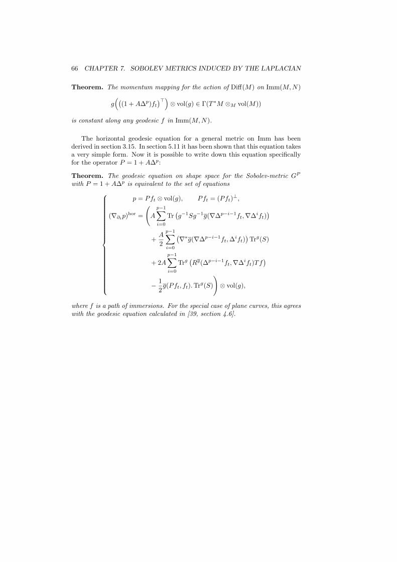
66 CHAPTER 7. SOBOLEV METRICS INDUCED BY THE LAPLACIAN
Theorem. The momentum mapping for the action of Diff(M) on Imm(M,N)
g((
(1 +A∆p)ft)>)⊗ vol(g) ∈ Γ(T ∗M ⊗M vol(M))
is constant along any geodesic f in Imm(M,N).
The horizontal geodesic equation for a general metric on Imm has beenderived in section 3.15. In section 5.11 it has been shown that this equation takesa very simple form. Now it is possible to write down this equation specificallyfor the operator P = 1 +A∆p:
Theorem. The geodesic equation on shape space for the Sobolev-metric GP
with P = 1 +A∆p is equivalent to the set of equations
p = Pft ⊗ vol(g), Pft = (Pft)⊥,
(∇∂tp)hor =
(A
p−1∑i=0
Tr(g−1Sg−1g(∇∆p−i−1ft,∇∆ift)
)+A
2
p−1∑i=0
(∇∗g(∇∆p−i−1ft,∆
ift))
Trg(S)
+ 2A
p−1∑i=0
Trg(Rg(∆p−i−1ft,∇∆ift)Tf
)− 1
2g(Pft, ft).Trg(S)
)⊗ vol(g),
where f is a path of immersions. For the special case of plane curves, this agreeswith the geodesic equation calculated in [39, section 4.6].

Chapter 8
Surfaces in n-space
This section is about the special case where the ambient space N is Rn. Theflatness of Rn leads to a simplification of the geodesic equation, and the Eu-clidean motion group acting on Rn induces additional conserved quantities. Thevector space structure of Rn allows to define a Frechet metric. This metric willbe compared to Sobolev metrics. Finally in section 8.5 the space of concentrichyper-spheres in Rn is briefly investigated.
Most of the material presented here can also be found in [8].
8.1 Geodesic equation
The covariant derivative ∇g on Rn is but the usual derivative. Therefore thecovariant derivatives ∇∂tft and ∇∂tp in the geodesic equation can be replacedby ftt and pt, respectively. (Note that Imm(M,Rn) is an open subset of theFrechet vector space C∞(M,Rn).) Also, the curvature terms disappear becauseRn is flat. Any of the formulations of the geodesic equation presented so far canthus be adapted to the case N = Rn.
We want to show how the geodesic equation simplifies further under theadditional assumptions that dim(M) = dim(N) − 1 and that M is orientable.Then it is possible define a unit vector field ν to M . The condition that ft ishorizontal then simplifies to Pft = a.ν for a ∈ C∞(M). The geodesic equationcan then be written as an equation for a. However, the equation is slightlysimpler when it is written as an equation for a.vol(g). In practise, vol(g) canbe treated as a function on M because one can identify vol(g) with its densitywith respect to du1 ∧ . . . ∧ dun−1, where (u1, . . . , un−1) is a chart on M . Thusmultiplication by vol(g) does not pose a problem.
Theorem. The geodesic equation for a Sobolev-type metric GP on shape space
67

68 CHAPTER 8. SURFACES IN N -SPACE
Bi(M,Rn) with dim(M) = n− 1 is equivalent to the set of equations Pft = a.ν
∂t(a.vol(g)
)=
1
2g(
Adj(∇P )(ft, ft), ν)− 1
2g(Pft, ft)g
(Trg(S), ν
),
where f is a path in Imm(M,Rn) and a is a time-dependent function on M .
Proof. Applying g(·, ν) to the geodesic equation 5.11 on shape space in termsof the momentum one gets
∂t(a.vol(g)
)= ∂t g
(Pft ⊗ vol(g), ν
)= g(∇∂t
(Pft ⊗ vol(g)
), ν)
+ g(Pft ⊗ vol(g),∇∂tν
)=
1
2g(
Adj(∇P )(ft, ft), ν)− 1
2g(Pft, ft)g
(Trg(S), ν
)+ 0.
Let us spell this equation out in even more details for the H1-metric. Thisis the case of interest for the numerical examples in section 10.
Theorem. The geodesic equation on shape space Bi(M,Rn) for the Sobolev-metric GP with P = 1 +A∆ is equivalent to the set of equations
Pft = a.ν
∂t(a.vol(g)
)=(Ag0
2
(s, g(∇ft,∇ft)
)− Tr(L)
2
(‖ft‖2g +A ‖∇ft‖2g01⊗g
))vol(g),
where f is a path of immersions, a is a time-dependent function on M , s =g(S, ν) ∈ Γ(T 0
2M) is the shape operator, L = g−1s ∈ Γ(T 11M) is the Weingarten
mapping, and Tr(L) is the mean curvature.
Proof. The fastest way to get to this equation is to apply g(·, ν) to the geodesicequation on Imm from section 7.3. This yields
∂t(a.vol(g)
)=(ATr
(g−1.s.g−1g(∇ft,∇ft)
)+A
2
(∇∗g(∇ft, ft)
)Tr(L)
− 1
2g(Pft, ft).Tr(L)
)vol(g)
=(Ag0
2
(s, g(∇ft,∇ft)
)− A
2Trg
(g(∇2ft, ft)
)Tr(L)
− A
2Trg
(g(∇ft,∇ft)
)Tr(L)− 1
2g((1 +A∆)ft, ft
)Tr(L)
)vol(g)
=(Ag0
2
(s, g(∇ft,∇ft)
)− A
2Trg
(g(∇ft,∇ft)
)Tr(L)
− 1
2g(ft, ft
).Tr(L)
)vol(g).
Notice that the second order derivatives of ft have canceled out.

8.2. ADDITIONAL CONSERVED MOMENTA 69
8.2 Additional conserved momenta
If P is invariant under the action of the Euclidean motion group Rn o SO(n),then also the metric GP is in invariant under this group action and one getsadditional conserved quantities as described in section 3.10:
Theorem. For an operator P that is invariant under the action of the Euclideanmotion group Rn o SO(n), the linear momentum∫
M
Pftvol(g) ∈ (Rn)∗
and the angular momentum
∀X ∈ so(n) :
∫M
g(X.f, Pft)vol(g)
or equivalently
∫M
(f ∧ Pft)vol(g) ∈∧2Rn ∼= so(n)∗
are constant along any geodesic f in Imm(M,Rn). The operator P = 1 +A∆p
satisfies this property.
These momenta have also been calculated in [8, section 4.3].
8.3 Frechet distance and Finsler metric
This section can also be found in [8, section 5.6].
The Frechet distance on shape space Bi(M,Rn) is defined as
distBi∞ (F0, F1) = inf
f0,f1‖f0 − f1‖L∞ ,
where the infimum is taken over all f0, f1 with π(f0) = F0, π(f1) = F1. Asbefore, π denotes the projection π : Imm→ Bi. Fixing f0 and f1, one has
distBi∞(π(f0), π(f1)
)= inf
ϕ‖f0 ϕ− f1‖L∞ ,
where the infimum is taken over all ϕ ∈ Diff(M). The Frechet distance is relatedto the Finsler metric
G∞ : T Imm(M,Rn)→ R, h 7→∥∥h⊥∥∥
L∞.
Lemma. The pathlength distance induced by the Finsler metric G∞ providesan upper bound for the Frechet distance:
distBi∞ (F0, F1) ≤ distBi
G∞(F0, F1) = inff
∫ 1
0
‖ft‖G∞ dt,
where the infimum is taken over all paths
f : [0, 1]→ Imm(M,Rn) with π(f(0)) = F0, π(f(1)) = F1.

70 CHAPTER 8. SURFACES IN N -SPACE
Proof. Since any path f can be reparametrized such that ft is normal to f , onehas
inff
∫ 1
0
∥∥f⊥t ∥∥L∞ dt = inff
∫ 1
0
‖ft‖L∞ dt,
where the infimum is taken over the same class of paths f as described above.Therefore
distBi∞ (F0, F1) = inf
f‖f(1)− f(0)‖L∞ = inf
f
∥∥∥∥∫ 1
0
ftdt
∥∥∥∥L∞≤ inf
f
∫ 1
0
‖ft‖L∞ dt
= inff
∫ 1
0
∥∥f⊥t ∥∥L∞ dt = distBi
G∞(F0, F1).
It is claimed in [32, theorem 13] that d∞ = distG∞ . However, the proofgiven there only works on the vector space C∞(M,Rn) and not on Bi(M,Rn).The reason is that convex combinations of immersions are used in the proof,but that the space of immersions is not convex.
8.4 Sobolev versus Frechet distance
This section can also be found in [8, section 5.7].
It is a desirable property of any distance on shape space to be strongerthan the Frechet distance. Otherwise, singular points of a shape could movearbitrarily far away without increasing the distance much.
As the following result shows, Sobolev metrics of low order do not have thisproperty. The author and the authors of [8] believe that they have this propertywhen the order is high enough, but were not able to prove this.
Lemma. Let GP be a metric on Bi(M,Rn) that is weaker than or at least as
weak as a Sobolev Hp-metric with p < dim(M)2 + 1, i.e.
‖h‖GP ≤ C ‖h‖Hp = C
√∫M
g((1 + ∆p)h, h
)vol(g) for all h ∈ T Imm.
Then the Frechet distance can not be bounded by the GP -distance.
Proof. It is sufficient to prove the claim for P = 1 + ∆p. Let f0 be a fixedimmersion of M into Rn, and let f1 be a translation of f0 by a vector h oflength `. It will be shown that the Hp-distance between π(f0) and π(f1) isbounded by a constant 2L that does not depend on `, where π denotes theprojection of Imm onto Bi. Then it follows that the Hp-distance can not bebounded from below by the Frechet distance, and this proves the claim.
For small r0, one calculates the Hp-length of the following path of immer-sions: First scale f0 by a factor r0, then translate it by h, and then scale itagain until it has reached f1. The following calculation shows that under theassumption p < m/2 + 1 the immersion f0 can be scaled down to zero in finite

8.5. CONCENTRIC SPHERES 71
Hp-pathlength L. Let r : [0, 1]→ [0, 1] be a function of time with r(0) = 1 andr(1) = 0.
LGP
Imm
(r.f0
)=
∫ 1
0
√∫M
g(rt.(1 + (∆(r.f0)∗g)p
)(f0), rt.f0
)vol((r.f0)∗g
)dt
=
∫ 1
0
√∫M
r2t .g((
1 +1
r2p(∆f∗0 g)p
)(f0), f0
)rmvol
(f∗0 g)dt
=
∫ 0
1
√∫M
g((
1 +1
r2p(∆f∗0 g)p
)(f0), f0
)rmvol
(f∗0 g)dr =: L
The last integral converges if m−2p2 < −1, which holds by assumption. Scaling
down to r0 > 0 needs even less effort. So one sees that the length of the shrinkingand growing part of the path is bounded by 2L.
The length of the translation is simply `√rm0 Vol(f0) = O(rm/2) since the
Laplacian of the constant vector field vanishes. Therefore
distGP
Bi
(π(f0), π(f1)
)≤ distG
P
Imm(f0, f1) ≤ 2L.
8.5 Concentric spheres
This section can also be found in [8, section 6.6].
For a Sobolev type metric GP that is invariant under the action of the SO(n)on Rn, the set of hyper-spheres in Rn with common center 0 is a totally geodesicsubspace of Bi(S
n−1,Rn). The reason is that it is the fixed point set of the groupSO(n) acting on Bi isometrically. (One also needs uniqueness of solutions tothe geodesic equation to prove that the concentric spheres are totally geodesic.)This section mainly deals with the case P = 1 + ∆p.
First we want to determine under what conditions the set of concentricspheres is geodesically complete under the GP -metric.
Lemma. The space of concentric spheres is complete with respect to the GP
metric with P = 1 +A∆p iff p ≥ (n+ 1)/2.
Proof. The space is complete if and only if it is impossible to scale a spheredown to zero or up to infinity in finite GP path-length. So let f be a pathof concentric spheres. It is uniquely described by its radius r. Its velocity isft = rt.ν, where ν designates the unit normal vector field. One has
g(g−1.S, ν
)=: L = − 1
r IdTM , Tr(Lk) = (−1)k n−1rk, Vol = rn−1 nπn/2
Γ(n/2+1) .
Keep in mind that r and rt are constant functions on the sphere, so that all

72 CHAPTER 8. SURFACES IN N -SPACE
derivatives of them vanish. Therefore
∆ν = ∇∗(∇ν) = ∇∗(−Tf.L) = Trg(∇(Tf.L)
)= Trg
(∇(Tf).L
)+ Trg
(Tf.(∇L)
)= Tr(L2).ν + Trg
(Tf.∇(− 1
r IdTM ))
=n− 1
r2.ν + 0
and
Pft = (1 +A∆p)(rt.ν) = rt.
(1 +A
(n− 1)p
r2p
).ν.
From this it is clear that the path f is horizontal. Therefore its length as a pathin Bi is the same as its length as a path in Imm. One calculates its length asin the proof of 8.4:
LGP
Bi(f) =
∫ 1
0
√GPf (ft, ft)dt =
∫ 1
0
√∫M
r2t .
(1 +A
(n− 1)p
r2p
)vol(g)dt
=
∫ 1
0
|rt|
√(1 +A
(n− 1)p
r2p
)n.πn/2
Γ(n/2 + 1)rn−1dt
=
√n.πn/2
Γ(n/2 + 1)
∫ r1
r0
√(1 +A
(n− 1)p
r2p
)rn−1dr.
The integral diverges for r1 → ∞ since the integrand is greater than r(n−1)/2.It diverges for r0 → 0 iff (n − 1 − 2p)/2 ≤ −1, which is equivalent to p ≥(n+ 1)/2.
The geodesic equation within the space of concentric spheres reduces to anODE for the radius that can be read off the geodesic equation in section 7.3:
rtt = −r2t
(n− 1
2r− p.A.(n− 1)p
r(r2p +A(n− 1)p
)).
Chapter 9
Diffeomorphism groups
For M = N the space Emb(M,M) equals the diffeomorphism group of M . Anoperator P ∈ Γ
(L(TEmb;TEmb)
)that is invariant under reparametrizations
induces a right-invariant Riemannian metric on this space. Thus one gets thegeodesic equation for right-invariant Sobolev metrics on diffeomorphism groupsand well-posedness of this equation. To the authors knowledge, well-posednesshas so far only been shown for the special case M = S1 in [18] and for thespecial case of Sobolev order one metrics in [23]. Theorem 5.6 establishes thisresult for arbitrary compact M and Sobolev metrics of arbitrary order.
In the decomposition of a vector h ∈ TfEmb into its tangential and normalcomponents h = Tf.h> + h⊥, the normal part h⊥ vanishes. By the naturalityof the covariant derivative, S = ∇Tf vanishes as well. Thus on gets:
Theorem. The geodesic equation on Diff(M) is given byp = Pft ⊗ vol(g),
∇∂tp = −Tf.g(Pft,∇ft)] ⊗ vol(g).
Note that this equation is not right-trivialized, in contrast to the equationgiven in [5, 37, 35], for example.
73

74 CHAPTER 9. DIFFEOMORPHISM GROUPS

Chapter 10
Numerical results
This section can also be found in [8, section 7].
It is of great interest for shape comparison to solve the boundary value prob-lem for geodesics in shape space. When the boundary value problem can besolved, then any shape can be encoded as the initial momentum of a geodesicstarting at a fixed reference shape. Since the initial momenta all lie in the samevector space, this also opens the way to statistics on shape space.
There are two approaches to solving the boundary value problem. In [7] thefirst approach of minimizing horizontal path energy over the set of curves in Immconnecting two fixed boundary shapes has been taken. This has been done forseveral almost local metrics. For these metrics it is straightforward to calculatethe horizontal energy because the horizontal bundle equals the normal bundle.However, in the case of Sobolev type metrics the horizontal energy involves theinverse of a differential operator (see section 5.8), which makes this approachmuch harder.
The second approach is the method of geodesic shooting. This method isbased on iteratively solving the initial value problem while suitably adaptingthe initial conditions. The theoretical requirements of existence of solutions tothe geodesic equation and smooth dependence on initial conditions are met forSobolev type metrics, see section 5.6. This makes geodesic shooting a promisingapproach.
The first step towards this aim is to numerically solve the initial value prob-lem for geodesics, at least for the H1-metric and the case of surfaces in R3, andthat is what will be presented in this work.
The geodesic equation on shape space is equivalent to the horizontal geodesicequation on the space of immersions. For the case of surfaces in R3, it takesthe form given in section 8.1. This equation can be conveniently set up usingthe DifferentialGeometry package incorporated in the computer algebra systemMaple as demonstrated in figure 10.1. (The equations that have actually beensolved were simplified by multiplying intermediate terms with suitable powersof√
vol(g), but for the sake of clearness this has not been included in the Maple
75

76 CHAPTER 10. NUMERICAL RESULTS
code in figure 10.1.)
Unfortunately, Maple (as of version 14) is not able to solve PDEs with morethan one space variable numerically. Thus the equations were translated intoMathematica. The PDE was solved using the method of lines. Spatial discretiza-tion was done using an equidistant grid, and spatial derivatives were replacedby finite differences. The time-derivative ft appears implicitly in the equationPf (ft) = a.ν, and this remains so when the operator Pf is replaced by finitedifferences.
The solver that has been used is the Implicit Differential-Algebraic (IDA)solver that is part of the SUNDIALS suite and is integrated into Mathematica.IDA uses backward differentiation of order 1 to 5 with variable step widths.Order 5 is standard and has also been used here. At each time step, the newvalue of ft is computed using some previous values of f , and then the new valueof f is calculated from the equation Pf (ft) = a.ν. The dependence on f inthis equation is of course highly nonlinear. A Newton method is used to solveit. This operation is quite costly and has to be done at every step, which isa main disadvantage of backward differentiation algorithms. Explicit methodsare probably much better adapted to the problem. The implementation ofan explicit solver is ongoing work of Martin Bauer, Martins Bruveris and theauthor. The results are too preliminary to be included in this thesis.
In the examples that follow, f at time zero is a square [0, π] × [0, π] flatlyembedded in R3. This is a manifold with boundary, but it can be seen as apart of a bigger closed manifold. Zero boundary conditions are used for both fand a. It remains to specify an initial condition for a. As a first example, letus assume that a at time zero equals sin(x) sin(y), where x, y are the Euclideancoordinates on the square. The resulting geodesic is depicted in figure 10.2.In the absence of a closed-form solution of the geodesic equation, one way tocheck if the solution is correct is to see if the energy GP (ft, ft) is conserved.Figure 10.3 shows this for the geodesic from figure 10.2 with various space andtime discretizations.
A more complicated example of a geodesic is shown in figure 10.4 and 10.5.There, the initial velocity was chosen to be a smoothened version of a blackand white picture of the letter A. The initial momentum was computed from itusing a discrete Fourier transform.
Finally, it is shown in figure 10.6 that self-intersections of the surface canoccur. This is not due to a numerical error but part of the theory, and can bean advantage or a disadvantage depending on the application.
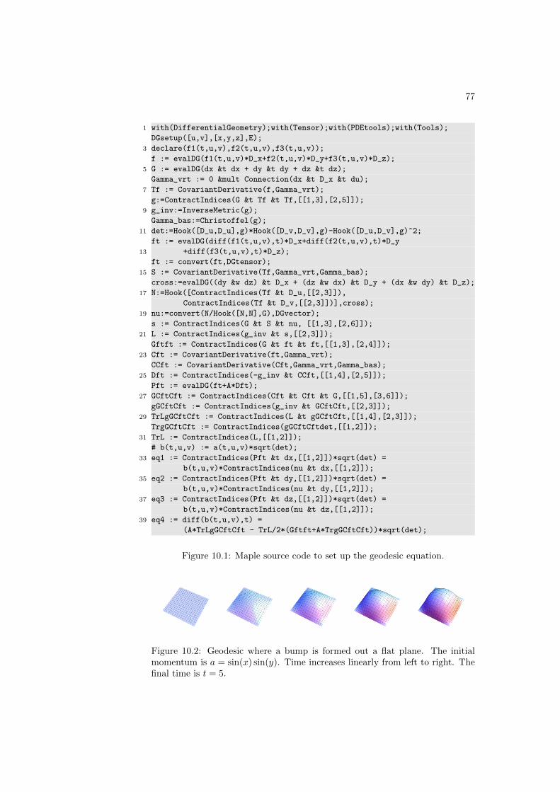
77
1 with(DifferentialGeometry);with(Tensor);with(PDEtools);with(Tools);
DGsetup([u,v],[x,y,z],E);
3 declare(f1(t,u,v),f2(t,u,v),f3(t,u,v));
f := evalDG(f1(t,u,v)*D_x+f2(t,u,v)*D_y+f3(t,u,v)*D_z);
5 G := evalDG(dx &t dx + dy &t dy + dz &t dz);
Gamma_vrt := 0 &mult Connection(dx &t D_x &t du);
7 Tf := CovariantDerivative(f,Gamma_vrt);
g:=ContractIndices(G &t Tf &t Tf,[[1,3],[2,5]]);
9 g_inv:=InverseMetric(g);
Gamma_bas:=Christoffel(g);
11 det:=Hook([D_u,D_u],g)*Hook([D_v,D_v],g)-Hook([D_u,D_v],g)^2;
ft := evalDG(diff(f1(t,u,v),t)*D_x+diff(f2(t,u,v),t)*D_y
13 +diff(f3(t,u,v),t)*D_z);
ft := convert(ft,DGtensor);
15 S := CovariantDerivative(Tf,Gamma_vrt,Gamma_bas);
cross:=evalDG((dy &w dz) &t D_x + (dz &w dx) &t D_y + (dx &w dy) &t D_z);
17 N:=Hook([ContractIndices(Tf &t D_u,[[2,3]]),
ContractIndices(Tf &t D_v,[[2,3]])],cross);
19 nu:=convert(N/Hook([N,N],G),DGvector);
s := ContractIndices(G &t S &t nu, [[1,3],[2,6]]);
21 L := ContractIndices(g_inv &t s,[[2,3]]);
Gftft := ContractIndices(G &t ft &t ft,[[1,3],[2,4]]);
23 Cft := CovariantDerivative(ft,Gamma_vrt);
CCft := CovariantDerivative(Cft,Gamma_vrt,Gamma_bas);
25 Dft := ContractIndices(-g_inv &t CCft,[[1,4],[2,5]]);
Pft := evalDG(ft+A*Dft);
27 GCftCft := ContractIndices(Cft &t Cft &t G,[[1,5],[3,6]]);
gGCftCft := ContractIndices(g_inv &t GCftCft,[[2,3]]);
29 TrLgGCftCft := ContractIndices(L &t gGCftCft,[[1,4],[2,3]]);
TrgGCftCft := ContractIndices(gGCftCftdet,[[1,2]]);
31 TrL := ContractIndices(L,[[1,2]]);
# b(t,u,v) := a(t,u,v)*sqrt(det);
33 eq1 := ContractIndices(Pft &t dx,[[1,2]])*sqrt(det) =
b(t,u,v)*ContractIndices(nu &t dx,[[1,2]]);
35 eq2 := ContractIndices(Pft &t dy,[[1,2]])*sqrt(det) =
b(t,u,v)*ContractIndices(nu &t dy,[[1,2]]);
37 eq3 := ContractIndices(Pft &t dz,[[1,2]])*sqrt(det) =
b(t,u,v)*ContractIndices(nu &t dz,[[1,2]]);
39 eq4 := diff(b(t,u,v),t) =
(A*TrLgGCftCft - TrL/2*(Gftft+A*TrgGCftCft))*sqrt(det);
Figure 10.1: Maple source code to set up the geodesic equation.
Figure 10.2: Geodesic where a bump is formed out a flat plane. The initialmomentum is a = sin(x) sin(y). Time increases linearly from left to right. Thefinal time is t = 5.

78 CHAPTER 10. NUMERICAL RESULTS
0.8225
0.8230
0.8235
0.8240
0.8245
0.8250
1 2 3 4 5
GP (ft, ft)
t
Figure 10.3: Conservation of the energy GP (ft, ft) along the geodesic in fig-
ure 10.2. The true value of GP (ft, ft) is π2
4(1+2A) ≈ 0.822467 for A = 1. The
maximum time step used in blue and green is 0.1. For purple and cyan it is0.05. The number of grid points used in blue and cyan is 100 times 100. Forgreen and purple it is 200 times 200.
Figure 10.4: Letter A forming along a geodesic path. Time increases linearlyfrom left to right. The final time is t = 0.8. Top and bottom row are differentviews of the same geodesic.
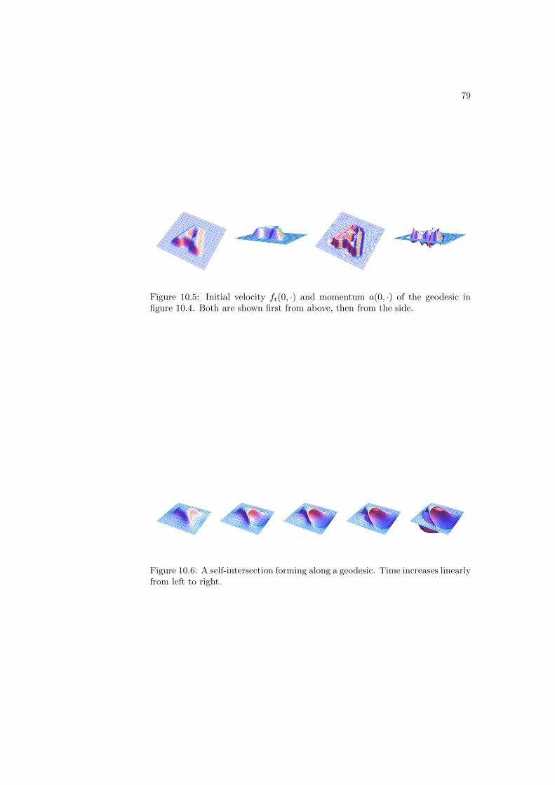
79
Figure 10.5: Initial velocity ft(0, ·) and momentum a(0, ·) of the geodesic infigure 10.4. Both are shown first from above, then from the side.
Figure 10.6: A self-intersection forming along a geodesic. Time increases linearlyfrom left to right.

80 CHAPTER 10. NUMERICAL RESULTS

Bibliography
[1] H. Alt and L. J. Guibas. Discrete geometric shapes: Matching, interpola-tion, and approximation: A survey. Technical Report B 96-11, EVL-1996-142, Institute of Computer Science, Freie Universitat Berlin, 1996.
[2] L. Ambrosio, N. Gigli, and G. Savare. Gradient flows with metric anddifferentiable structures, and applications to the wasserstein space. AttiAccad. Naz. Lincei Cl. Sci. Fis. Mat. Natur. Rend. Lincei (9) Mat. Appl.,15(3-4), 2004.
[3] L. Ambrosio, N. Gigli, and G. Savare. Gradient flows in metric spaces andin the space of probability measures. Lectures in Mathematics ETH Zurich.Birkhauser Verlag, Basel, second edition, 2008.
[4] F. Arman and J. Aggarwal. Model-based object recognition in dense-rangeimages—a review. ACM Comput. Surv., 25(1):5–43, 1993.
[5] V. I. Arnold. Sur la geometrie differentielle des groupes de lie de dimensioninfinie et ses applications a l’hydrodynamique des fluides parfaits. Ann.Inst. Fourier, 16:319–361, 1966.
[6] R. Bajcsy, R. Lieberson, and M. Reivich. A computerized system for theelastic matching of deformed radiographic images to idealized atlas images.J. Comput. Assisted Tomogr., 7:618–625, 1983.
[7] M. Bauer, P. Harms, and P. W. Michor. Almost local metrics on shapespace of hypersurfaces in n-space, 2010. URL arXiv:math/1001.0717.
[8] M. Bauer, P. Harms, and P. W. Michor. Sobolev metrics on shape spaceof surfaces in n-space, 2010. URL arXiv:math/1009.3616.
[9] M. Bauer, P. Harms, and P. W. Michor. Curvature weighted metrics onshape space of hypersurfaces in n-space. http://www.mat.univie.ac.at/
~michor/gauss-surfaces.pdf, 2010.
[10] Martin Bauer. Almost local metrics on shape space of surfaces. PhD thesis,University of Vienna, 2010.
[11] M. F. Beg, M. I. Miller, A. Trouve, and L. Younes. Computing largedeformation metric mappings via geodesic flows of diffeomorphisms. Int.J. Comput. Vision, 61(2):139–157, 2005.
81

82 BIBLIOGRAPHY
[12] J.-D. Benamou, Y. Brenier, and K. Guittet. The Monge-Kantorovitchmass transfer and its computational fluid mechanics formulation. Internat.J. Numer. Methods Fluids, 40(1-2):21–30, 2002.
[13] Jean-David Benamou and Yann Brenier. A computational fluid mechanicssolution to the Monge-Kantorovich mass transfer problem. Numer. Math.,84(3):375–393, 2000.
[14] P. J. Besl and R. C. Jain. Three-dimensional object recognition. Comput.Surv., 17(1):75–145, March 1985.
[15] Arthur L. Besse. Einstein manifolds. Classics in Mathematics. Springer-Verlag, Berlin, 2008.
[16] Fred L. Bookstein. Morphometric tools for landmark data : geometry andbiology. Cambridge University Press, 1997.
[17] V. Cervera, F. Mascaro, and P. W. Michor. The action of the diffeomor-phism group on the space of immersions. Differential Geom. Appl., 1(4):391–401, 1991.
[18] Adrian Constantin and Boris Kolev. Geodesic flow on the diffeomorphismgroup of the circle. Comment. Math. Helv., 78(4):787–804, 2003.
[19] S. Durrleman, X. Pennec, A. Trouve, P. Thompson, and N. Ayache. In-ferring brain variability from diffeomorphic deformations of currents: anintegrative approach. Med Image Anal, 12(5):626–637, 2008.
[20] S. Durrleman, X. Pennec, A. Trouve, and N. Ayache. Statistical modelsof sets of curves and surfaces based on currents. Med Image Anal, 13(5):793–808, 2009.
[21] Jurgen Eichhorn. Global analysis on open manifolds. Nova Science Pub-lishers Inc., New York, 2007.
[22] Jurgen Eichhorn and Jan Fricke. The module structure theorem for Sobolevspaces on open manifolds. Math. Nachr., 194:35–47, 1998.
[23] Francois Gay-Balmaz. Well-posedness of higher dimensional Camassa-Holm equations. Bull. Transilv. Univ. Brasov Ser. III, 2(51):55–58, 2009.
[24] J. Glaunes, A. Qiu, M. I. Miller, and L. Younes. Large deformation diffeo-morphic metric curve mapping. Int. J. Comput. Vision, 80(3), 2008.
[25] D. Holm, A. Trouve, and L. Younes. The Euler-Poincare theory of meta-morphosis. Quart. Appl. Math., 67(4):661–685, 2009.
[26] David G. Kendall. Shape-manifolds, procrustean metrics, and complexprojective spaces. Bull. London Mathematical Society, 16:81–121, 1984.
[27] Shoshichi Kobayashi and Katsumi Nomizu. Foundations of differential ge-ometry. Vol. I. Wiley Classics Library. John Wiley & Sons Inc., New York,1996.
[28] I. Kolar, P. W. Michor, and J. Slovak. Natural operations in differentialgeometry. Springer-Verlag, Berlin, 1993.

BIBLIOGRAPHY 83
[29] Andreas Kriegl and Peter W. Michor. The convenient setting of globalanalysis, volume 53 of Mathematical Surveys and Monographs. AmericanMathematical Society, Providence, RI, 1997.
[30] Sergey Kushnarev. Teichons: solitonlike geodesics on universal Teichmullerspace. Experiment. Math., 18(3):325–336, 2009.
[31] S. Loncaric. A survey of shape analysis techniques. Pattern Recognition,31(8):983–1001, 1998.
[32] A. Mennucci, A. Yezzi, and G. Sundaramoorthi. Properties of Sobolev-typemetrics in the space of curves. Interfaces Free Bound., 10(4):423–445, 2008.
[33] M. Micheli, P. W. Michor, and D. Mumford. Sectional curvature in terms ofthe cometric, with applications to the riemannian manifolds of landmarks.,2010. URL arXiv:1009.2637.
[34] Peter W. Michor. Manifolds of differentiable mappings. Shiva Publ., 1980.
[35] Peter W. Michor. Some geometric evolution equations arising as geodesicequations on groups of diffeomorphisms including the Hamiltonian ap-proach. In Phase space analysis of partial differential equations, vol-ume 69 of Progr. Nonlinear Differential Equations Appl., pages 133–215.Birkhauser Boston, 2006.
[36] Peter W. Michor. Topics in differential geometry, volume 93 of GraduateStudies in Mathematics. American Mathematical Society, Providence, RI,2008.
[37] Peter W. Michor and David Mumford. Vanishing geodesic distance onspaces of submanifolds and diffeomorphisms. Doc. Math., 10:217–245 (elec-tronic), 2005.
[38] Peter W. Michor and David Mumford. Riemannian geometries on spacesof plane curves. J. Eur. Math. Soc. (JEMS) 8 (2006), 1-48, 2006. URLarxiv:math/0312384.
[39] Peter W. Michor and David Mumford. An overview of the Riemannianmetrics on spaces of curves using the Hamiltonian approach. Appl. Comput.Harmon. Anal., 23(1):74–113, 2007.
[40] M. I. Miller, A. Trouve, and L. Younes. On the metrics and euler-lagrangeequations of computational anatomy. Annu Rev Biomed Eng, 4:375–405,2002.
[41] A. R. Pope. Model-based object recognition: A survey of recent research.Technical Report TR-94-04, University of British Columbia, January 1994.
[42] E. Sharon and D. Mumford. 2d-shape analysis using conformal mapping.In Proc. IEEE Conf. Computer Vision and Pattern Recognition, pages 350–357, 2004.
[43] E. Sharon and D. Mumford. 2d-shape analysis using conformal mapping.International Journal of Computer Vision, 70:55–75, 2006.

84 BIBLIOGRAPHY
[44] M. A. Shubin. Pseudodifferential operators and spectral theory. SpringerSeries in Soviet Mathematics. Springer-Verlag, Berlin, 1987.
[45] D’Arcy Thompson. On Growth and Form. Cambridge University Press,1942.
[46] Alain Trouve and Laurent Younes. Diffeomorphic matching problems inone dimension: Designing and minimizing matching functionals. In DavidVernon, editor, Computer Vision, volume 1842. ECCV, 2000.
[47] Alain Trouve and Laurent Younes. Metamorphoses through Lie group ac-tion. Found. Comput. Math., 5(2):173–198, 2005.
[48] Marc Vaillant and Joan Glaunes. Surface matching via currents. In In-formation Processing in Medical Imaging, volume 3565 of Lecture Notes inComputer Science, pages 381–392. Springer Berlin / Heidelberg, 2005.
[49] R. C. Veltkamp and M. Hagedoorn. State-of-the-art in shape matching.Technical Report UU-CS-1999-27, Utrecht University, 1999.
[50] Steven Verpoort. The geometry of the second fundamental form: Curva-ture properties and variational aspects. PhD thesis, Katholieke UniversiteitLeuven, 2008.
[51] L. Younes, P. W. Michor, J. Shah, and D. Mumford. A metric on shapespace with explicit geodesics. Atti Accad. Naz. Lincei Cl. Sci. Fis. Mat.Natur. Rend. Lincei (9) Mat. Appl., 19(1):25–57, 2008.
[52] Laurent Younes. Computable elastic distances between shapes. SIAM J.Appl. Math., 58(2):565–586 (electronic), 1998.
Zusammenfassung
Zusammenfassung. Geometrische Figuren spielen eine wichtige Rolle in vie-len Bereichen der Wissenschaft, Technik und Medizin. Mathematisch kann eineFigur als unparametrisierte, immersive Teil-Mannigfaltigkeit modelliert werden,was auch der dieser Arbeit zugrunde liegende Figurenbegriff ist. Wenn der Raumder Figuren mit einer Riemannschen Metrik ausgestattet wird, eroffnet sichdie Welt der Riemannschen Differential-Geometrie mit Geodaten, Gradienten-Flussen und Krummung. Leider induziert die einfachste solche Metrik verschwin-dende Kurvenlangen-Distanz am Raum der Figuren. Diese Entdeckung von Mi-chor und Mumford war der Ausgangspunkt fur die Suche nach starkeren Metri-ken, die es ermoglichen sollten, Figuren anhand von fur die jeweilige Anwendungwichtigen Merkmalen zu unterscheiden. Sobolev-Metriken sind ein vielverspre-chender Ansatz dazu. Es gibt sie in zwei Varianten: Sogenannte außere Me-triken, die von Metriken auf der Diffeomorphismen-Gruppe des umgebendenRaums induziert werden, und innere Metriken, die intrinsisch zur Figur defi-niert sind. In dieser Arbeit werden innere Sobolev-Metriken in einem sehr all-gemeinen Rahmen entwickelt und prasentiert. Es gibt keine Einschrankung aufdie Dimension des eingebetteten oder umgebenden Raums, und der umgebendeRaum muss nicht flach sein. Es wird gezeigt, dass die Kurvenlangen-Distanzvon inneren Sobolev Metriken am Raum der Figuren nicht verschwindet. DieGeodatengleichung und die durch Symmetrien erzeugten Erhaltungsgroßen wer-den hergeleitet, und die Wohldefiniertheit der Geodatengleichung wird gezeigt.Beispiele von numerischen Losungen der Geodatengleichung schließen die Arbeitab.
85

86 APPENDIX

Curriculum Vitae
Personal Data
Name: Philipp Harms
Email: [email protected]
Nationality: Austria
Date of birth: 25. 07. 1984
Place of birth: Graz
Education
2008–2010 Ph.D. in MathematicsUniversity of Vienna
2003–2008 Master in Mathematics, with distinctionVienna University of Technology
2004–2006 Studies of Lutheran Theology,University of Vienna
1996–2002 A-level, with distinctionAkademisches Gymnasium Graz
Conferences and research visits
October, 2010 Imperial College, London: Research visit
July, 2010 Scuola Normale Superiore di Pisa: Research visit
July, 2010 Curves and Surfaces, Avignon: Conference
May, 2010 Shape FRG, London: Conference
January, 2010 Winter School Geometry and Physics, Srni:Conference
September, 2009 Shape modelling group at CNR IMATI-GE, Genova:Research visit
June, 2009 Ecole Normale Superieure de Cachan, Paris:Research visit
87

88 APPENDIX
April 2009 Shape FRG, Annapolis, MD: Conference
January, 2009 Winter School Geometry and Physics, Srni:Conference
Teaching experience
2005-2007 Mathematics 1, 2 and 3 in mechanical engineering,Mathematics 1 in computer scienceVienna University of Technology
Publications and Preprints
Preprint: Geodesics in infinite dimensional Stiefel and Grass-mann manifolds
Preprint: Curvature weighted metrics on shape space of sur-faces in n-space
Preprint: Sobolev metrics on shape space
Preprint: Almost local metrics on shape space of surfaces inn-space
Master Thesis: The Poincare Lemma in Subriemannian Geometry
November 25, 2010

![Lesson 3 Symbols of the United States - Sarasotamoaa 3 Symbols of US[2]-r1.pdfAnnuit Coeptis is over the eye and translates to mean, “He has favored our undertakings.” The date](https://img.dokumen.tips/doc/110x75/5e4def330d296f2205373c40/lesson-3-symbols-of-the-united-states-sarasotamoaa-3-symbols-of-us2-r1pdf-annuit.jpg)


![Continental Congress of the newlyship, introduced the mottos Annuit Coeptis (He [God] has favored our undertakings) over the eye and Novus Ordo Seclorum (A Secretary of Congress Charles](https://img.dokumen.tips/doc/110x75/5e4dec3ae949ab131c2dfd09/continental-congress-of-the-newly-ship-introduced-the-mottos-annuit-coeptis-he.jpg)


![The Morse-Smale Complex - univie.ac.atmichor/schaetz_dipl.pdfThe Morse-Smale Complex ... For an exposition of Morse Theory as a toy-model of infinite-dimensional issues, see [16],](https://img.dokumen.tips/doc/110x75/5edc26afad6a402d6666b1e8/the-morse-smale-complex-michorschaetzdiplpdf-the-morse-smale-complex-for.jpg)