Disincentives from Redistribution: Evidence on a Dividend

WU International Taxation Research Paper Series

No. 2019 - 05

Disincentives from Redistribution: Evidence on a Dividend of Democracy

Rupert Sausgruber

Axel Sonntag

Jean-Robert Tyran

Editors:

Eva Eberhartinger, Michael Lang, Rupert Sausgruber and Martin Zagler (Vienna University of

Economics and Business), and Erich Kirchler (University of Vienna)

Electronic copy available at: https://ssrn.com/abstract=3475358

1

Disincentives from Redistribution:

Evidence on a Dividend of Democracy

Rupert Sausgruber, Axel Sonntag, and Jean-Robert Tyran*

31 May 2019

Abstract

We experimentally study the disincentive effect of taxing work and

redistributing tax revenues when redistribution is imposed vs. democratically

chosen in a vote. We find a “dividend of democracy” in the sense that the

disincentive effect is substantially smaller when redistribution is chosen in a

vote than when it is imposed. Redistribution seems to be more legitimate, and

hence less demotivating, when accepted in a vote.

Keywords: Redistribution, disincentive effect, voting, legitimacy, real-

effort task, lab experiment

JEL codes: C92, D31, D72, H23

* Sausgruber: Vienna University of Economics and Business, [email protected]; Sonntag: University of Vienna and IHS Vienna, [email protected]; Tyran: University of Vienna, University of Copenhagen and CEPR London, [email protected]. We thank Mads Harmsen and Arno Parolini for effective research assistance and Ralph Bayer, Lydia Mechtenberg and Adam Zylbersztejn, as well as seminar participants at Columbia U, NYU, Brown U, VSE Prague, HU Berlin, U Vienna, U Copenhagen and BSB Dijon for helpful comments. We are grateful to the Austrian Science Fund under project number I2027-G16 for financial support.


2

1 Introduction

One of the most fundamental issues in economics is the trade-off between equity and efficiency:

having a more equitable society typically comes at a cost. For example, redistributing labor

income to reduce inequality can involve losses in efficiency due to a disincentive effect, which

occurs when work is discouraged because it is taxed (MaCurdy 1992; Ziliak and Kniesner 1999;

Kumar 2008). However, the severity of this trade-off is hotly debated. Estimates of

the responsiveness of labor supply to changes in taxes vary widely (Keane 2011; Saez, Slemrod,

and Giertz 2012). Our paper does not add another estimate but, to the best of our knowledge, is

the first to show that the responsiveness depends on whether people democratically choose to

be taxed. In particular, we show that the disincentive effect of taxation is more pronounced, and

thus leads to higher efficiency costs, if redistribution is imposed than if it is chosen in a vote.

That is, we demonstrate a “dividend of democracy” in redistribution.

To demonstrate this effect, we create a laboratory environment in which we observe a

substantial disincentive effect as follows. Participants earn money by working on a real-effort

task or consume leisure. In an initial phase, both work and leisure are untaxed. In a second

phase, a tax on work but not on leisure is imposed, thus inducing disincentives to work. Tax

revenues are redistributed per capita. Using a difference-in-differences approach, we find

evidence of a substantive disincentive effect of imposed redistribution. In an otherwise identical

treatment, participants vote on whether to tax work at a given rate. We find that output falls by

much less (about two thirds less) when participants collectively choose to tax work than when

taxes are imposed exogenously.

This finding of a dividend of democracy in a redistribution context is novel, surprising, and

important. It is novel as previous experimental demonstrations of an endogeneity premium were

in the context of cooperation games (see below for references). Our finding is surprising as we

create a laboratory environment in which subjects earn their incomes through work which tends

to stack incentives against support for redistribution (Cappelen et al. 2007; Lefgren, Sims, and

Stoddard 2016). Our result is important because it indicates that the cost of redistribution can

be reduced by gathering democratic support for redistribution. We also find that due to reduced

disincentives, tax revenues are higher for a given tax rate when redistribution is chosen rather

than imposed. We argue that these findings obtain because chosen redistribution is perceived

as more legitimate and thus less demotivating than imposed redistribution (Tyler 1988; Castillo

2011; Peter 2009).

Our paper adds to the literature as follows.


3

First, we add to the literature on the disincentive effect. While there are many empirical

studies using administrative or field data (see Keane 2011 for a survey), only a few experimental

studies have addressed the problem (e.g., Agranov and Palfrey 2015). Our design stands out in

cleanly pinning down the disincentive effect in a real-effort task with proportional tax and per

capita redistribution.1

Second, our paper adds to the literature on the endogeneity premium of economic policies.

Previous research provides suggestive evidence that it matters whether a policy is implemented

exogenously or democratically chosen in a vote (e.g., Grossman and Baldassarri 2012). While

we are the first to find an endogeneity premium in voting on taxation and redistribution, several

lab studies have found an endogeneity premium in different contexts. For example, Alm,

McClelland, and Schulze (1999) find that voting in a tax enforcement context conveys

information about the underlying social norm in addition to its instrumental value. Voting is

also found to increase the acceptance and effectiveness of sanctioning mechanisms (Tyran and

Feld 2006; Putterman, Tyran, and Kamei 2011; Markussen, Putterman, and Tyran 2014; Kamei

2016). In a real-effort workplace setting, letting subjects choose between payment schemes

increased exerted effort (Mellizo, Carpenter, and Matthews 2014). People also seem to value

having decision rights over and above their instrumental value (Bartling, Fehr, and Herz 2014).

However, the evidence on the endogeneity premium is not uniform. For example, Gallier (2018)

and Vollan et al. (2017) fail to find evidence of an endogeneity premium.

The closest match to our study is Dal Bó, Foster, and Putterman (2010, henceforth DFP).

Using a clever design to control for selection effects in social dilemma games, they find

increased cooperation when voters choose to modify the game than when such a modification

is imposed. We use an approach similar to DFP to quantify selection vs. causal effects (see

section 4) and we find that the causal effect - by a factor of 40 - dominates the selection effect.

Our findings are related to results from empirical studies on the effects of democratic

institutions. For example, participation rights reduce tax evasion (Torgler 2005) and the size of

the shadow economy (Teobaldelli and Schneider 2013, for further aspects see Acemoglu et al.

1 Our findings relate to the literature on redistribution and social preferences (e.g., Alesina and Angeletos 2005; Fong 2001; Fong, Bowles, and Gintis 2005; Tyran and Sausgruber 2006), the literature comparing endogenous and exogenous games (e.g., Charness, Fréchette, and Qin 2007), and the literature on uncertainty and voting (e.g., Bird 2001; Frohlich and Oppenheimer 1990; Ortona et al. 2008). We also provide a new angle on the discussion of the determinants of successful welfare states. Many explanations have been put forward to account for differences in how well welfare states work, e.g., the 'civicness' of people or transparency (Algan, Cahuc, and Sangnier 2016; Luttmer and Singhal 2014). We add one, namely whether or not people have a say on implementing redistribution.


4

2019; Feld, Fischer, and Kirchgässner 2010; Frey and Stutzer 2005; Torgler 2002). Acemoglu

et al. (2015, p. 1886f) conclude that “the existing empirical literature is … full of contradictory

results” and therefore “very far from a consensus on the relationship between democracy,

redistribution, and inequality”.

Third, we develop a new experimental task that provides interior rather than corner

solutions, enabling us to predict optimal labor supply responses to changes in incentives (see

our companion paper Haeckl, Sausgruber, and Tyran 2018). In contrast, the tasks commonly

used, such as adjusting slider positions or transcriptions, tend to be non-responsive to changes

in economic incentives (see Gächter, Huang, and Sefton 2016 for a notable exception).

The paper proceeds as follows: Section 2 presents the experimental design and section 3

contains the results. Section 4 discusses selection effects vs. dividend of democracy and section

5 concludes.

2 Experimental Design

Figure 1 illustrates the structure of the experiment. The basic building block is a phase

consisting of 20 minutes in which participants either work in a real-effort task or consume

leisure.2 Both activities provide income to participants. If participants work in the real-effort

task, they are paid a piece rate. If participants consume leisure, they are paid a constant rate per

second. In phase 1, neither income from work nor leisure is taxed (condition NoR). Phase 2 is

the same as phase 1, except that income from work (but not leisure) may be taxed at a flat rate

and tax revenues are redistributed per capita within a group. There are two treatments, which

differ by how the decision to redistribute is taken after phase 1 has been completed.

In treatment Endo, the group decides by simple majority vote whether or not to tax labor

income and redistribute it in phase 2. Before knowing the outcome of the vote, i.e., before

knowing whether work is taxed in phase 2, participants state their expectations for both

contingencies. That is, they state how much they expect to work themselves and how much the

other group members are going to work given that redistribution is implemented or not.

2 It is well known from the experimental literature that subjects’ sense for responsibility and deservingness is of key importance in redistributive settings (e.g., Cappelen, Sørensen, and Tungodden 2010). That is why we used a real-effort to generate the pre-tax income distributions as opposed to e.g., randomly drawing them. We want to avoid participants to perceive the initial distribution to be correlated to luck as this may be of importance to subjects' behavior (e.g., Almas et al. 2010). The induced sense of entitlement should result in a particularly strong disincentive effect of redistribution, because it is less legitimate (Durante, Putterman, and van der Weele 2014; Cappelen, Konow, et al. 2013). That is why the obtained treatment differences are particularly impressive and provide a strong test for the effect of democracy.


5

Treatment Exo is the same as Endo, except that participants do not vote. Redistribution is

exogenously and randomly imposed on groups in this case. Participants know when they state

their expectations in Exo that they are equally likely assigned to a condition with redistribution

(condition R) or without redistribution (NoR).

We identify the disincentive effect in a difference-in-differences approach. In treatment

Exo, the first difference (D) refers to the difference in individual �’s output before and after

redistribution: �� , �� ,��. The second difference refers to the difference

between phases in the control treatment without redistribution, i.e., �� , �� ,��. The difference between the two measures identifies the average disincentive effect in

case of exogenous redistribution, i.e., �� . The

corresponding measure for treatment Endo, ��, is constructed analogously. The

dividend of democracy is then identified by �� . However,

subjects in Endo choose whether to have redistribution or not which means that selection may

matter. We discuss this issue further in section 0.

Figure 1: Experimental design

Parameters and procedures

At the beginning of a session, participants are randomly assigned to groups of three participants

each. Group composition remains constant for the entire experiment (partner matching

protocol). Participants are told that the experiment will have several parts, and that they will be

informed later about the specifics of these parts. That is, subjects do not know until the end of

phase 1 that the experiment may involve redistribution (unless otherwise specified, all


6

information provided below is common information; the experimental instructions are in

Appendix A1).

Phase 1 is identical in both treatments. In phase 1, subjects work by calculating single-digit

cross sums or consume leisure individually for 20 minutes. Neither work nor leisure is taxed,

and incomes are not redistributed in phase 1. Subjects earn a piece rate of 1 point per correct

cross sum. Cross sums become increasingly difficult to calculate over time. The first 15 cross

sums consist of two single digits (e.g., 2 + 4 = ?) and a digit is added after every 15th cross sum,

so the task becomes more difficult as subjects progress (e.g., 8 + 9 + 4 + 2 + 1 + 5 + 7 + 8 + 9

+ 1 = ?). Subjects have the option to switch to a “leisure mode” at any point in time during the

20 minute interval by clicking on a button.3 Once in the leisure mode subjects can not switch

back to the work task for the rest of the phase and receive 1 point for every 15 seconds in the

leisure mode. Thus, in phase 1 it is profitable to work as long as calculating a cross sum takes

less than 15 seconds, and to switch to the leisure mode when it takes longer.

We choose this particular real-effort task because it is simple, easy to explain, and easy to

complete for our subjects (who are all undergraduate students). But by adding digits over time,

work becomes increasingly tedious. The main purpose of this novel task is to increase the

difficulty of the work task to induce subjects to stop working and to switch into the leisure

mode. The advantage of our procedure is that we prevent subjects from being in a corner

solution (i.e., they worked for 20 minutes) which implies that changes in relative prices do

trigger a behavioral response. Interior solutions make observing disincentive (i.e., substitution)

effects from taxation more likely.4 Other work tasks used in related studies typically suffer from

a lack of responsiveness of work effort to changes in incentives and therefore are unsuitable for

our purposes.

We are not the first to provide workers with opportunity cost of work by offering a paid

alternative to effort provision (Erkal, Gangadharan, and Nikiforakis 2011; Berger, Harbring,

3 Each screen presents three cross-sums and subjects proceed to the next screen by clicking an ok button (see Appendix A1 for a screenshot). If individuals provide a wrong answer, the program indicates which one needs to be corrected to move on to the next screen. In the instructions, the work task is neutrally referred to as the “cross-sum task” while the leisure mode is called “switch task”. However, we use the expressions “tax” and “redistribution” in the instructions. Subjects answer control questions and participate in an unpaid trial round before phase 1 starts. Screens also indicate the remaining time and the number of correct answers at the time. In the leisure mode subjects see a clock ticking and an indication of their income earned.

4 Our design successfully induces such interior solutions. In fact, the average subject stops working after about 15 minutes and 99.2% of all subjects work less than 20 minutes in phase 1. This contrasts with many real effort experiments in which dramatic changes of incentives have little effects. For example in Cappelen et al. (2013b, 2010) a doubling of the piece rate has essentially no significant effect on output (copying a text). The same is true for the real-effort ball catching task in Gächter et al. (2016). In conditions without induced monetary costs of catching balls, doubling the gains for success did not change behavior.


7

and Sliwka 2013; Mohnen, Pokorny, and Sliwka 2008; Weber and Schram 2017; Goerg, Kube,

and Radbruch 2017).5 However, we are, to the best of our knowledge, the first to use a task with

induced monetary opportunity cost of work to measure disincentives of taxation and

redistribution (see also our companion paper on work motivation in teams: Haeckl, Sausgruber,

and Tyran 2018).

At the end of phase 1, subjects receive feedback on the outcomes of phase 1. They are

reminded of their own leisure time and their own output (i.e., the number of correct cross sums)

and receive information about the leisure time and output of the other two group members. We

then distribute new instructions explaining the rest of the experiment including the

redistribution scheme of phase 2.

Phase 2 is the same as phase 1, i.e., subjects work on the same cross-sum task or consume

leisure for 20 minutes, except that income from work may be taxed and the revenues

redistributed. With the redistribution scheme, income from work is taxed at a flat rate of 60%

(but income from leisure remains untaxed). All tax revenues are redistributed per capita. Since

a group has three members, the net tax rate is 40%. Subjects know whether the redistribution

scheme applies to their group at the beginning of phase 2 before they start to work.

In treatment Endo, subjects vote whether or not a redistribution scheme applies, while in

treatment Exo a random draw (with 50% chance) decides. In treatment Endo, subjects vote on

redistribution. Voting is anonymous, costless and compulsory (yes or no, abstentions are not

allowed). The decision is taken by simple majority vote. That is, redistribution is implemented

if at least 2 voters approved of the proposal. Subjects learn the outcome of the vote before phase

2 starts (but not how many individuals vote for redistribution). We carefully explain the

mechanics of how changes in own income from leisure (which is untaxed), changes in own pre-

tax income from work, and changes in the income distribution translate into changes in post-

redistribution incomes. In addition, a profit calculator is available to calculate each member’s

payoff for given expected output levels and leisure consumption.

Before the decision on redistribution is made, subjects have to indicate their expectations

about the outcomes in phase 2 both for the case with redistribution (condition R) and the case

without redistribution (condition NoR). When they indicate expectations, they know the

properties of the redistribution scheme and the outcomes for phase 1 in their group. In

5 In addition there are also several papers offering unpaid alternatives (e.g., Abeler et al. 2011; Charness, Masclet, and Villeval 2014; Corgnet, Hernán-González, and Rassenti 2015; Kessler and Norton 2016) or the option to leave the lab (Dickinson 1999; Rosaz, Slonim, and Villeval 2016). We cannot use either of these alternatives as we need monetary opportunity cost in order to predict money-maximizing behavior.


8

particular, subjects state expectations for their own and the other two group members’ outcomes

in phase 2.6 We elicit expectations at this point, because any observable differences in

disincentive effects may be due to a differential change in beliefs. By eliciting beliefs before

phase 2, we can control for such an anticipated dividend of democracy.

Experimental sessions are conducted at the laboratory of the University of Copenhagen

using zTree (Fischbacher 2007). In total, 240 undergraduate students (180 in Endo and 60 in

Exo) from various fields are recruited using ORSEE (Greiner 2015). During the experiment,

subjects earn incomes in points which are converted a rate of 3 points = 2 DKK (1 point ~

€0.08) and paid out at the end of the experiment. Sessions last approximately 110 minutes and

average earnings are around €23. No participation fee is paid.

Redistribution provides clear disincentives to work in our design. With redistribution, it is

profitable to switch to the leisure task earlier than without. Instructions explain in detail that a

subject should switch if calculating a cross sum takes more than 9 seconds with redistribution

rather than more than 15 seconds without redistribution. The reason for switching sooner with

redistribution is that the net income per cross sum falls from 1 to 0.6 (= 1 - 40% net tax), see

Appendix A1 for instructions. Subjects are also informed that they would decrease their own

income if they work longer than optimal. We also explain in detail that subjects with above-

average output will be net losers from redistribution, and vice-versa for those for below-average

output.

3 Results

First, we discuss labor supply in phase 1, i.e., absent redistribution. Second, we show that

redistribution caused a strong disincentive effect in treatment Exo, output falls by about one

third. Third, we show that the disincentive effect of redistribution is much smaller when it is

endogenously chosen in a vote than when it is exogenously imposed (output falls by about

12%).

Labor supply absent redistribution (phase 1)

Figure 2 shows the distribution of output in phase 1 across all 240 subjects. We merge the data

across treatments because phase 1 is identical in Endo and Exo and, reassuringly, we find that

6 Estimates of others’ output are incentivized. Subjects receive additional 50 points if their expectation is within the range of +/- 7 points of the true value. Estimates of own output are not incentivized to prevent misreporting due to “hedging” (Blanco et al. 2010).


9

the distribution of output across treatments is not different (p = 0.994, Kruskal-Wallis test). The

average subject calculates 105.6 cross sums and switches to the leisure task after about 15

minutes (846.1 seconds, to be precise; see Appendix A2 for further descriptive statistics). There

is considerable variation in phase 1 outputs across subjects which is essential when studying

redistribution (note that our redistribution scheme has no effect on the secondary income

distribution when subjects are equal ex ante).7

Figure 2: Output in phase 1

We find that average labor supply is fairly close to optimal in phase 1. In particular, the

average deviation from the optimal stopping time per screen is -4.0 seconds, which corresponds

to a deviation of about -1.3 seconds per cross sum (i.e., about 9% of the optimal stopping time).8

The observation that average labor supply is so close to optimal suggests that subject were

motivated by money and that the incentives were clear to them (cf. Abeler and Jäger 2015).

Note that a rational subject has no reason to deviate from optimal labor supply in phase 1. The

7 The overall primary income distribution is not skewed in our experiment as is typical for naturally occurring wage distributions (with many workers earning low wages and few earning very high wages). A skewed distribution of primary incomes implies a high degree of equilibrium redistribution in standard models (e.g., Meltzer and Richard 1981). One might thus expect a relatively low level of support for redistribution in our experiment. However, redistribution is not implemented on the population level but within groups that are randomly sampled from this distribution. As a consequence, many group-level distributions are indeed skewed, thus leading to considerable demand for redistribution.

8 All numbers on stopping time reported here refer to screens because we measure the time when a subject clicks to move to the next screen. The deviation from optimal stopping time is measured as described in Appendix A5. If a subject stops without ever crossing the threshold of 45 seconds per screen, we take the time of the last working screen. If she stops after having crossed the threshold at least for one period, we take the average time of all periods between the period just before crossing the threshold for the first time and period when stopping to work altogether.

05

10

15

Perc

ent

0 50 100 150 200

Completed tasks in phase 1

Average: 105.6

Median: 108.0

S.dev. = 31.7

n = 240


10

reason is that there is no redistribution, which means that subjects’ choices have no externalities

whatsoever in phase 1 by design.

Figure 3: Output for selected individuals

Note: Cumulated output of three selected individuals who stopped working at different times. Diamond: Highly

productive subject (stops late). Circle: less productive subject (stops early). Triangle: subject with intermediate

productivity. If all subjects stopped optimally, the horizontal distance between the two most right observations per

subject in the figure above should be the same for all subjects, namely 15 seconds, independent of their individual

productivity.

Figure 3 shows cumulated output and work times for three selected subjects of different

productivity. Productivity refers to the speed with which cross sums are calculated. For

example, after about 4 minutes of work (see Figure 4: vertical dashed line at 250 seconds) the

least productive worker has completed just below 50 cross sums while the most productive

worker has completed more than 70. The concavity of the production function is induced by

the increasing difficulty of the real-effort task (additional digits are added to the cross-sum task

over time), meaning that completing cross sums takes increasingly more time. It is optimal for

more productive workers to stop working later, and for less productive workers to stop earlier.

Concavity also implies that the disincentive effect (i.e., the reaction to a change in the relative

price of work and leisure) is stronger in absolute terms for more productive workers than for

less productive workers.

050

100

150

Cum

ula

ted n

um

ber

of

tasks

0 250 500 750 1000 1250

Cumulated work time [in seconds]


11

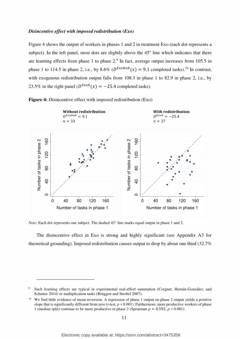
Disincentive effect with imposed redistribution (Exo)

Figure 4 shows the output of workers in phases 1 and 2 in treatment Exo (each dot represents a

subject). In the left panel, most dots are slightly above the 45° line which indicates that there

are learning effects from phase 1 to phase 2.9 In fact, average output increases from 105.5 in

phase 1 to 114.5 in phase 2, i.e., by 8.6% (�� 9.1 completed tasks).10 In contrast,

with exogenous redistribution output falls from 108.3 in phase 1 to 82.9 in phase 2, i.e., by

23.5% in the right panel (�� 25.4 completed tasks).

Figure 4: Disincentive effect with imposed redistribution (Exo)

Without redistribution

�� 9.1

� � 33

With redistribution

�� 25.4

� � 27

Note: Each dot represents one subject. The dashed 45° line marks equal output in phase 1 and 2.

The disincentive effect in Exo is strong and highly significant (see Appendix A3 for

theoretical grounding). Imposed redistribution causes output to drop by about one third (32.7%

9 Such learning effects are typical in experimental real-effort summation (Corgnet, Hernán-González, and Schniter 2014) or multiplication tasks (Brüggen and Strobel 2007).

10 We find little evidence of mean reversion. A regression of phase 1 output on phase 2 output yields a positive slope that is significantly different from zero (t-test, p < 0.001). Furthermore, more productive workers of phase 1 (median split) continue to be more productive in phase 2 (Spearman � � 0.592, p < 0.001).

040

80

12

016

0

Nu

mb

er

of

tasks in p

ha

se 2

0 40 80 120 160

Number of tasks in phase 1

040

80

12

016

0

Nu

mb

er

of

tasks in p

ha

se 2

0 40 80 120 160



12

to be exact, �� 34.5 completed tasks).11 Responses in ExoR and ExoNoR are

significantly different (�� . ��, p < 0.001, Wilcoxon ranksum test,

henceforth WRS). Given the strong increase in taxation (from 0 to 40%), this reaction

corresponds to a labor supply elasticity of about 0.8 (= 32.7% / 40%). This elasticity is, perhaps

surprisingly, broadly consistent with estimates of labor supply elasticities from field data.

Keane (2011) reports Hicks elasticities from 0.02 to 1.32 for males, and from 0.77 to 1.6 for

females (sum of elasticities at extensive and intensive margin).

This pronounced disincentive effect results from most subjects stopping to work earlier,

rather than working less intensely or stopping to work altogether. Redistribution causes subjects

to reduce work time by -50.6% (��! � ��! � ��! � �310.6 � 95.0 ��405.5 seconds, �� ! � . ��!, p = 0.001, WRS).

The disincentive effect in Exo translates into a substantial reduction of output and

incomes.12 The redistribution scheme has two effects on labor income. Figuratively speaking,

it ‘shrinks the pie’ and redirects incomes from more productive to less productive workers,

meaning that less productive workers get a ‘larger share of the pie’. However, the net effect of

getting a larger share of a smaller pie is unclear. To study this issue we rank the workers in each

group according to their phase 1 output and calculate the average income per rank over all

groups. As expected, we find that the incomes of the most productive workers tend to fall (by

35.8%, p < 0.001, WRS). Moreover, the labor incomes of the middle-ranked workers fall by

42.5% (p = 0.001, WRS). Finally, also the incomes of the least productive workers on average

fall by 20.0% (p = 0.060, WRS), i.e., overall, the least productive workers, by getting a bigger

share of the smaller pie, cannot improve their post-redistribution labor incomes.

A dividend of democracy (Endo vs. Exo)

Figure 5 shows the disincentive effect with endogenous redistribution, i.e., when subjects vote

on whether to implement the redistributive scheme. In total, 42.7% of workers vote in favor of

11 All comparisons hold the set of subjects constant by treatment and redistribution condition across phases. For example, the behavior of subjects who are assigned to ExoR in phase 2 is compared to their own behavior in phase 1. Unless otherwise stated, all statistical tests are one-sided (because we hold directional hypotheses) and non-parametric tests are at the group level to control for dependence at the group level.

12 Inequality-reducing redistribution may increase welfare for various reasons. For example, the marginal utility of income may be higher for the poor than for the rich, or workers may be averse to inequality. In addition, the material costs of the disincentive effect are likely to overestimate the overall costs of redistribution because there are gains in leisure. We discuss this aspect in more detail in Appendix A10.


13

redistribution and the scheme is accepted in 35% of the cases.13 The disincentive effect in Endo

is measured analogously to the one in Exo. Absent redistribution, we observe moderate learning

effects in terms of output (�� = 1.5 completed tasks). In the groups that do accept

redistribution, output falls by �� = -11.0 completed tasks. Thus, the disincentive effect

when redistribution is accepted in a vote is �� = -12.5 completed tasks, which is

equivalent to a significant fall in output by 11.8% (�� . ��, p = 0.006,

WRS).

We find evidence for a dividend of democracy: the disincentive effect in Endo is smaller

than in Exo. In fact, �� = -12.5 and �� = -34.5 completed tasks. This dividend

is an endogeneity premium in the sense that output falls less when redistribution has been

chosen in a vote than when it is exogenously imposed. In fact, the disincentive effect with

democratic redistribution is only about a third of the disincentive effect with imposed

redistribution (��/�� 36.1%), and the disincentive effect is significantly

different across treatments (�� 22.1 completed tasks, p =

0.007, z-test, see regression analysis in Table 1, part Diff-in-diff-in-diff).14 As a consequence,

the cost of redistribution in terms of lost labor income is smaller with endogenous than

exogenous redistribution (for heterogeneous effects regarding productivity see Appendix A11).

In Exo, we found that the net effect of getting a larger share of a smaller pie is strongly

negative. In Endo, the most productive workers and those with intermediate productivity lose

labor income from redistribution (-20.8%, p < 0.001 and -0.1%, p = 0.028, respectively, WRS),

while the least productive workers are equally well off with and without redistribution (0.0%,

p = 0.252, respectively, WRS).

13 We focus on the consequences of (exogenous vs. endogenous) redistribution and therefore do not discuss the determinants of voting in much detail. Suffice it to note that voting is broadly in line with elicited beliefs about expected gains from redistribution (85% and 75% of yes and no voters, respectively, see Table 2).

14 Note that it is not meaningful to compare two difference-in-differences measures with non-parametric tests (since vectors degenerate to scalars, this would mean comparing two numbers). For that reason, we conducted regression analyses for all comparisons of DD measures. Unless otherwise stated all z-tests are two-sided.


14

Figure 5: Disincentive effect with endogenous redistribution (Endo)


�� 1.51 � � 117

With redistribution

�� 10.95

� � 63

Notes: Each dot represents one subject. The dashed 45° line marks equal output in phase 1 and 2. The disincentive effect is much less pronounced in EndoR than in ExoR (see right panel of Figure 4). For additional separation by individual voting behavior see Appendix A4.

Note that in EndoNoR (Figure 5, left panel) a greater proportion of observations lie below

the 45° line than in ExoNoR (Figure 4, left panel, p = 0.027, Fisher’s exact test). That is, output

increases by less in Endo than in Exo absent redistribution (p = 0.035, WRS). A possible

explanation of this difference is that subjects who improve their performance less than others

select via voting into the NoR condition in Endo, whereas subjects are randomly assigned in

Exo. While plausible, selection via voting cannot explain this difference in output change. In

fact, there is no difference between yes- and no-voters in terms of change of output from phase

1 to 2 (p = 0.142 and p = 0.432 in NoR and R, respectively, two-sided Fisher’s exact test).

Oversupply of work

While knowing that a dividend of democracy prevails is novel, surprising and important, as

explained in the introduction, it is also interesting from a scientific perspective to know why

exactly it obtains, i.e., what the determinants of the premium are. The rest of this section argues

that the endogeneity premium prevails because subjects in groups that endogenously accepted

redistribution in phase 2 tend to oversupply work, while this behavioral pattern is not present

in any of the other conditions.

040

80

12

016

0

Nu

mb

er

of

tasks in p

ha

se 2

0 40 80 120 160


40

80

12

016

0

Nu

mb

er

of

tasks in p

ha

se 2

0 40 80 120 160



15

Endogenous redistribution has strikingly different effects on output when it is chosen rather

than imposed because redistribution affects work time differently in the two cases. We call

work duration in excess of the optimal stopping time ‘overtime’. When redistribution is chosen,

subjects do almost three times as much overtime (per screen) than when redistribution is

imposed: ��! � !∗ � 38.3 seconds vs. ��! � !∗ � 13.4 seconds, with ��! �!∗ � 24.9 seconds (p = 0.028, z-test, see Table 1). Note that while the privately optimal labor

supply falls with redistribution (recall it is optimal to stop after 9 rather than 15 seconds),

socially optimal labor supply remains unaffected. The reason is that what is taken from one

person is given to another, i.e., there are no direct costs or benefits of redistribution to society

(no ‘leaky-bucket effect’ or efficiency gains in our design). The result above therefore implies

that efficiency falls less with endogenous than with exogenous redistribution.

A further consequence of oversupply of work is that the tax revenue, and hence

redistribution, is higher in Endo than in Exo. In fact, we find for our given tax rate 12% higher

tax revenues when it is chosen rather than imposed (avg. tax revenue is 55.7 vs. 49.7 points, p

= 0.049, WRS).

Table 1 shows that regression analysis confirms our non-parametric results.15 In particular,

we find clear evidence of a disincentive effect both in ExoR and EndoR (in terms of output and

worktime), but the disincentive effect is substantially smaller in EndoR. This is so because

subjects work much longer when redistribution is chosen rather than imposed. The top third

contains results for treatment Exo, the middle part for treatment Endo, and the bottom part the

difference of the two (which we call the diff-in-diff-in-diff).

Column 1 shows the respective results for output, i.e., the number of completed tasks. In

Exo, subjects who did not get redistribution in phase 2 (ExoNoR), on average completed 105.45

tasks in phase 1, see row (i). Subjects in groups who got redistribution in phase 2 (ExoR) on

average completed 2.88 tasks more than those in ExoNoR in phase 1, but this difference is not

significant, indicating a successful random allocation of subjects into treatment conditions.

Subjects in ExoNoR became slightly more productive over time, i.e., they completed on average

9.09 tasks more in phase 2 than in phase 1. In contrast, subjects in ExoR completed 25.45 tasks

less in phase 2 than in phase 1. That is, in total, we find a substantial and significant disincentive

15 In Table 1 we report results obtained from multi-level regressions (with hierarchical error clustering: subjects nested in groups), but the results are robust to different error specifications (clustering error only on group level).


16

effect in Exo (�� 25.45 � 9.09 � �34.54), see row

(iv).

In Endo, subjects in groups that did not select into redistribution in phase 2 on average

completed 105.85 tasks, see row (v). Again, randomization was successful, since output is not

significantly different from those who did select into redistribution, see row (vii). Subjects in

EndoNoR completed on average 1.51 tasks more in phase 2 than in phase 1, but this increase

in output is not significant. In contrast, subjects in EndoR completed on average 10.96 tasks

less in phase 2 than in phase 1. Thus, in total, we find a significant disincentive effect in Endo

(�� 10.96 � 1.51 � �12.47), see row (viii).

The bottom third of Table 1 shows results of the diff-in-diff-in-diff (DDD) analysis that

sheds light on the differences between the treatments Exo and Endo. Row (i) – (v) indicates that

subjects in condition NoR completed on average 0.39 tasks less over time in Exo than in Endo.

This non-significant difference again indicates successful randomization. Row (ii) – (vi) shows

that the output of subjects in condition R increased their output over time by 7.58 tasks more in

Exo than in Endo. Hence, there are no differential learning effects between Exo and Endo. Row

(iii) – (vii) again indicates that randomization was successful. Finally, row (iv) – (viii) shows

our main result: the difference in the disincentive effect between chosen and imposed

redistribution. Subjects reduced their output by 22.07 tasks less in EndoR than in ExoR.

Columns 2, 3 and 4 of Table 1 are constructed analogously and show the results for

worktime (number of seconds subjects spent on completing tasks), productivity (number of

tasks completed within the first five minutes of a phase) and overtime (deviation from optimal

stopping time).

Column 2 shows that subjects stop working earlier in conditions with redistribution than

without. While this is true for both Exo and Endo, the disincentive effect on worktime is much

stronger when redistribution is imposed rather than chosen in a vote. In fact, subjects stop

working over 4 minutes (245.58 seconds) earlier in ExoR than in EndoR, see row (iv) – (viii).

Column 3 shows that there is no a difference in productivity between impose and chosen

redistribution, see row (iv) – (viii).


17

Table 1: Regression analysis

(1) (2) (3) (4) Output Worktime Productivity a) Overtime b)

Treatment EXO

(i) constant 105.45*** 783.36*** 215.76*** -10.47**

(5.12) (52.83) (6.34) (5.26)

(ii) phase 9.09* 94.97* 4.85 3.94

(4.81) (54.55) (6.74) (6.47)

(iii) redistribution 2.88 41.82 -0.94 2.61

(7.63) (78.75) (9.45) (7.84)

(iv) phase x redistribution -34.54*** -405.54*** -22.26** 13.41 (7.16) (81.32) (10.05) (9.64)

Observations 120 120 120 120 Log. Likelihood -564.77 -848.73 -595.35 -573.52 Chi-squared 31.07 35.24 8.25 8.53

Treatment ENDO

(v) constant 105.85*** 850.23*** 204.62*** -3.97

(2.97) (29.84) (3.96) (3.03)

(vi) phase 1.51 -17.85 7.95*** 1.02

(2.46) (32.60) (2.47) (3.46)

(vii) redistribution -1.99 29.96 -5.73 4.94

(5.01) (50.45) (6.70) (5.12)

(viii) phase x redistribution -12.47*** -159.95*** -7.31* 38.30***

(4.16) (55.10) (4.18) (5.84)


Diff-in-diff-in-diff

(i)-(v) constant -0.39 -66.88 11.14 -6.50 (6.16) (62.70) (7.94) (6.28)

(ii)-(vi) phase 7.58 112.82* -3.10 2.92 (5.30) (67.65) (5.95) (7.36)

(iii)-(vii) redistribution 4.87 11.86 4.78 -2.33 (9.47) (96.35) (12.20) (9.66)

(iv)-(viii) phase x redistribution -22.07*** -245.58** -14.94 -24.89** (8.14) (103.96) (9.14) (11.31)


Notes: All columns show coefficients of multi-level regressions (with hierarchical error clustering: subjects nested in groups); standard errors in parentheses; levels of significance: * p < 0.1, ** p < 0.05, *** p < 0.01 a) Productivity is measured as number of completed tasks per second within the first five minutes of a phase (coefficients are multiplied by 1000 for better visibility). b) Overtime is defined as the difference between actual and optimal stopping time, averaged across all observations as from just before the optimal stopping time was exceeded for the first time. For more details and a graphical example see Appendix A5.

In Appendix A6 we also show separate regression tables for yes and no voters, respectively.


18

Column 4 shows a substantial and highly significant difference in overtime between ExoR

and EndoR. Worktime in Exo is close to optimal with and without redistribution (no significant

difference in overtime: ��! � !∗ � 13.41 seconds), see row (iv). In contrast, worktime

in Endo deviates strongly from optimality with redistribution, but not without. As a

consequence, overtime is significantly higher with chosen redistribution (��! � !∗ �38.30 seconds), see row (viii). Overall, overtime is 24.89 seconds higher with chosen than with

imposed redistribution, see row (iv) – (viii).

4 Disentangling the endogeneity effect: selection vs. dividend of democracy

Our design isolates causal effects of redistribution and disincentives on labor supply in Exo but

not in Endo. The reason is that unobserved characteristics might be correlated both with higher

output and with voting for redistribution in Endo.16 Therefore, the endogeneity effect, i.e., the

finding that disincentives are less pronounced if redistribution is accepted in a vote rather than

imposed, can be both driven by selection or causation. In fact, workers select into EndoR via

voting which may, in turn, be influenced by their characteristics. As a result of selection, the

distribution of characteristics may be different in the two conditions and these characteristics

may determine production. Hence, the observed difference in output between the endogenous

and exogenous conditions may partly be due to differences in subjects’ characteristics rather

than to a causal effect of voting. Some of these characteristics can be directly observed by the

researcher, for some characteristics proxies can be found, others might remain unobserved.

To illustrate, suppose prosocial subjects are more likely to vote for redistribution. If

prosocial subjects tend to work harder than others we will find that output is higher with

endogenous choice than it would have been with random allocation as in Exo. The dividend of

democracy claims that voting has a causal effect on disincentives. While selection produces a

difference in average behavior across redistribution conditions because prosocial subjects are

represented in different proportions in EndoR and EndoNoR, the causal effect obtains because

the subjects that happen to be in the redistribution condition change their behavior.

We investigate the relative importance of selection vs. the dividend of democracy in three

steps. First, we discuss individual voting and find that selection effects may be present.

However, we show in a second step that selection is not the main driver of the endogeneity

16 In contrast to Dal Bó, Foster, and Putterman (2010), we do not identify the pure endogeneity effect by directly conditioning on voting behavior both in Endo and Exo, because in our design subjects only vote in Endo.


19

effect. The reason is that the output of a particular worker is much more driven by whether

redistribution is accepted by his or her group than by whether he or she voted for redistribution.

Third, we adapt the framework by Dal Bó, Foster, and Putterman (2010) to quantify the relative

size of the selection effect and find that it is very small. We conclude by discussing possible

causes of why the dividend of democracy obtains.

Individual voting

This section shows that voting was predominantly in line with material self-interest and that the

deviations from it are significantly different for subjects who expect to gain vs. lose. Therefore,

voting may in principle have induced selection effects.

Table 2: Voting by subjects who expect to gain or lose versus actual gain or loss (Endo)

Vote Expect to gain Expect to lose Grand total

Actual gain

Actual loss

Total Actual gain

Actual loss

Total

Yes 32 13 45 9 23 32 77

No 4 4 8 19 76 95 103

Total 36 17 53 28 99 127 180

Notes: Subjects indicated their beliefs about both possible group outcomes in phase 2, i.e., with and without redistribution, at the end of phase 1. Expected gain/loss was computed for each subject using these beliefs. Actual gain/loss is the difference between observed and counterfactual income of each subject in phase 2. Counterfactual is estimated on the basis of regression analysis.

Table 2 shows voting decisions in Endo. Whether subjects “expect to gain” vs. “expect to

lose” is calculated from the beliefs subjects indicate before the vote for both possible outcomes,

i.e., for EndoR and EndoNoR. We calculate the actual gain and loss by comparing the subjects’

observed income with the counterfactual income. For example, for a subject who is in a group

that accepted redistribution, we take the subject’s observed income with redistribution and

subtract his or her counterfactual income without redistribution. Counterfactual income is

calculated from regression analysis. To illustrate, the number in the upper left corner shows that

32 subjects expect to gain, vote yes and gain from redistribution. Some of these 32 subjects end

up in EndoR, in which case their counterfactual is calculated for EndoNoR and vice versa (this

difference is not shown in Table 2 but available on request).

Table 2 shows that voting is predominantly in line with expectations, assuming that voters

are rational and self-interested. In particular, the share of yes-voters among those who expect

to gain is 85% (= 45/53), and the share of no-voters among those who expect to lose is 75% (=


20

95/127). We find that the proportion of those who deviate from self-interest is significantly

higher among those who expect to lose (25% = 32/127) than among those who expect to gain

(15% = 8/53, p < 0.046, ' -test). This asymmetry may explain the observed endogeneity effect

if voters who vote yes against their material self-interest were more productive than others.

However, we show that this is not the case in the next section.

Voting outcomes shape labor supply

We now show that voting choices have no motivational effects in the sense that they shape labor

supply, but that voting outcomes do. We find that those who are sorted into EndoR work harder

(i.e., work overtime) than those who are sorted into EndoNoR. Importantly, this motivational

effect occurs independent of their individual voting choices.

Table 3: Overtime in Phase 2 – Phase 1 in Endo, i.e., ��! � !∗

Outcome of the referendum is that redistribution proposal is

Accepted (R) Not Accepted (NoR)

Yes-Voters 42.57

(n = 43) 2.71

(n = 34)

No-Voters 32.35

(n = 20) 0.33

(n = 83)

Notes: Overtime is defined as the difference between actual and optimal stopping time per task, averaged across all observations as from just before the optimal stopping time was exceeded for the first time. For more details and a graphical example see Appendix A5.

Table 3 shows that selection effects are of minor importance, if any. To make our case, we

again refer to “overtime” as the difference between actual and optimal stopping time per task

(see section 3.3 for a discussion).

The first finding is that voters behave differently depending on the outcome of the vote.

This holds for both yes-voter and no-voters. In particular, we find that yes-voters in groups that

accept redistribution work significantly more overtime than those in groups that reject

redistribution (�� (). ��* = 42.57 - 2.71 = 39.86, p < 0.001, WRS). We also find that no-voters

who select into NoR work much less overtime than those who are ‘forced’ into R (�� (). ��

= 32.35 - 0.33 = 32.02, p < 0.001, WRS).

Moreover, we find that yes-voters who are ‘forced’ into NoR do not work more overtime

than no-voters who select into NoR (��* (). �� = 2.71 - 0.33 = 2.37, p = 0.428, two-sided

WRS). This finding speaks against selection effects if we assume that biased subjects (i.e., those

who irrationally work overtime no matter what) are more likely to vote yes (the converse test

is also not significant: ��* (). �� = 42.57 - 32.35 = 10.22, p = 0.585, two-sided WRS). In


21

conclusion of the discussion above, we do not find a significant effect of an unobserved

characteristic driving both voting and overtime. Selection effects, if any, must therefore be

small.

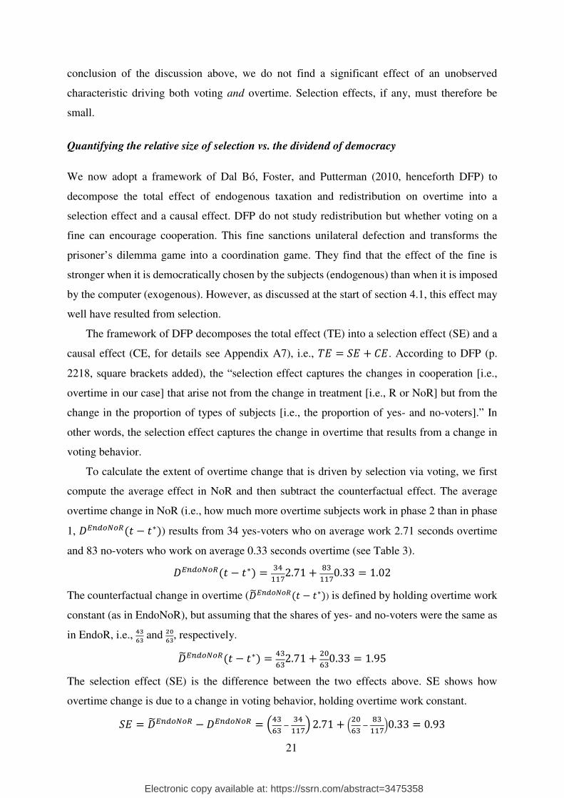
Quantifying the relative size of selection vs. the dividend of democracy

We now adopt a framework of Dal Bó, Foster, and Putterman (2010, henceforth DFP) to

decompose the total effect of endogenous taxation and redistribution on overtime into a

selection effect and a causal effect. DFP do not study redistribution but whether voting on a

fine can encourage cooperation. This fine sanctions unilateral defection and transforms the

prisoner’s dilemma game into a coordination game. They find that the effect of the fine is

stronger when it is democratically chosen by the subjects (endogenous) than when it is imposed

by the computer (exogenous). However, as discussed at the start of section 4.1, this effect may

well have resulted from selection.

The framework of DFP decomposes the total effect (TE) into a selection effect (SE) and a

causal effect (CE, for details see Appendix A7), i.e., +, � -, + /,. According to DFP (p.

2218, square brackets added), the “selection effect captures the changes in cooperation [i.e.,

overtime in our case] that arise not from the change in treatment [i.e., R or NoR] but from the

change in the proportion of types of subjects [i.e., the proportion of yes- and no-voters].” In

other words, the selection effect captures the change in overtime that results from a change in

voting behavior.

To calculate the extent of overtime change that is driven by selection via voting, we first

compute the average effect in NoR and then subtract the counterfactual effect. The average

overtime change in NoR (i.e., how much more overtime subjects work in phase 2 than in phase

1, ��! � !∗) results from 34 yes-voters who on average work 2.71 seconds overtime

and 83 no-voters who work on average 0.33 seconds overtime (see Table 3).

��! � !∗ � 01��22.71 + 30

��20.33 � 1.02

The counterfactual change in overtime (�4��! � !∗) is defined by holding overtime work

constant (as in EndoNoR), but assuming that the shares of yes- and no-voters were the same as

in EndoR, i.e., 5676 and 89

76, respectively.

�4��! � !∗ � 10:02.71 + ;

:00.33 � 1.95

The selection effect (SE) is the difference between the two effects above. SE shows how

overtime change is due to a change in voting behavior, holding overtime work constant.

-, � �4�� <10:0 = 01

��2> 2.71 + ? ;:0 = 30

��[email protected] � 0.93


22

The causal effect (CE) is calculated analogously, using condition R. We first compute the

average effect in R (��! � !∗) and then subtract the counterfactual effect. The average

overtime change in R results from 43 yes-voters who on average work 42.57 seconds overtime

and 20 no-voters who work on average 32.35 seconds overtime.

��! � !∗ � 10:042.57 + ;

:032.35 � 39.33

The counterfactual change in overtime (�4��! � !∗) is defined by holding the shares of

voters constant (as in EndoR), but assuming that overtime work was the same as in EndoNoR,

i.e., 2.71 and 0.33, respectively.

�4��! � !∗ � 10:02.71 + ;

:00.33 � 1.95

The causal effect (CE) is the difference between the two expressions above. CE shows how

overtime change is due to a behavioral change, holding voting proportions constant.

/, � �� 4�� 10:042.57 + ;

:032.35 � <10:02.71 + ;

:00.33> � 37.37

The total effect (TE) is the sum of SE and CE.

+, � -, + /, � 0.93 + 37.37 � 38.30

The decomposition above used the average treatment differences of Table 3 but is consistent

with our diff-in-diff analysis Table 1 (see Table 1, column 4, row viii).

In summary, applying the framework of DFP to our data results in a small selection effect

of 2.4% (= 0.93/38.30) and a large causal effect of 97.6% (= 37.37/38.30) of the total effect.17

The discussion above has used the framework of DFP to show that there is very little selection

on unobservables. This still leaves the possibility that there are selection effects on observable

characteristics that cancelled each other out. We investigate this possibility in great detail in

Appendix A8, but find no evidence for selection effects on observables.

In all, we conclude that the contribution of selection effects to the endogeneity effects is

minor and that the evidence for the dividend of democracy is strong.

Why the endogeneity premium may obtain

We believe that subjects who end up in EndoR behave differently than those in ExoR because

they observe their fellow group members’ (majoritarian) support for redistribution. This

information makes redistribution more legitimate in the eyes of the subjects than imposed

17 This small selection effect is consistent with an empirical analysis of selection on observables (failure to optimize, preference for inequality-aversion, underestimating the disincentive effect, insurance motive, see Appendix A8). See also Appendix A4 for a decomposed (by voting) version of Figure 5.


23

redistribution. We speculate that more legitimate redistribution is perceived to be less annoying

than less legitimate redistribution. This legitimacy effect might explain the smaller reduction in

output we observe in EndoR (-11.8%) than in ExoR (-32.7%).

DFP suggest two alternative explanations for why the democracy has an effect in their

experiment. The first operates indirectly, through expectations. According to this explanation,

learning that other subjects voted for the fine affects beliefs about how other subjects will

behave which, in turn, shapes their own behavior. The second explanation operates directly.

They speculate that “endogenous modification may strengthen the establishment of a

cooperative social norm or may operate as a coordination device” (DFP, p. 2221). They then

show that the first explanation “is not the main force behind the effect of democracy” (ibid.).

The speculation we provide above (the ‘legitimacy effect’) is more akin to DFP’s second

explanation. We therefore conclude that the underlying drivers of behavior in our experiment

may be similar to the ones in DFP.

We investigate several alternative explanations that could potentially account for our

endogeneity premium in Appendix A9. In particular, we examine inequality aversion,

reciprocity, conditional cooperation based on production beliefs, insurance motives, non-

optimizing behavior, and biased expectations regarding the magnitude of the disincentive

effect, and find no evidence in support for these explanations.

5 Conclusion

We show that democratically chosen redistribution is less harmful than exogenously imposed

redistribution because democratic choice not only affects whether redistribution is

implemented, but also shapes its consequences. It is well known that letting people vote on

whether or not to have redistribution is beneficial because of allocative efficiency (i.e., the

majority of voters get what they want). Our findings suggest that there is an additional benefit

from an endogeneity premium of voting. We find that even those who do not get what they

want are less annoyed if the decision is supported by the majority, perhaps because

redistribution is perceived as more legitimate.

In particular, we find in a laboratory experiment that the disincentive effect of imposed

redistribution (condition Exo) is large: subjects reduce the time spent working by about 50% if

they are forced into redistribution. As a consequence, output falls by roughly 33% in the

exogenous treatment. In contrast, democratic choice (condition Endo) cuts the negative impact

of redistribution to a mere 12% drop in output. In cases where no redistribution is implemented,

we observe no disincentive effects and indeed the output in EndoNoR and ExoNoR is not


24

different. In contrast, if the majority is in favor of redistribution, our results clearly indicate that

EndoR is less harmful than ExoR.

We suggest three avenues for further research.

First, it would be interesting to investigate how our results extrapolate to larger electorates.

Decisions taken in larger electorates allow for studying whether the margin of acceptance

shapes legitimacy (larger support may be perceived as more legitimate). Another aspect that

can be studied in larger electorates concerns expressive voting (e.g., Tyran 2004). Individual

voters have a negligible effect on the outcome (because of low pivotality) in large electorates.

As a consequence, material incentives of voting for one alternative over another are close to

zero and the (consumptive) utility of expressing support for one alternative or another may

come to dominate (Tyran and Wagner 2019 mention the “Brexit” referendum as an example).

Therefore, voters may support causes they do not really wish to win which, in turn, undermines

the legitimacy of the vote.

Second, we can only speculate on how our results may speak to the disincentive effects of

redistribution if redistribution choices are taken by some representative body (like a parliament)

rather than in a direct vote. The legitimacy of choices taken by representatives may depend on

various factors, e.g., on how well minorities are represented in parliament or whether the

parliamentary election process is perceived as being fair.

Third, it would worthwhile to explore how our results apply to continuous choice of tax

rates. We explore discrete choice of taxation at a net rate of 40%, i.e., voters only have the

choice to accept or reject redistribution at that rate. In experiments such as Agranov and Palfrey

(2015), each voter suggest a tax rate and the choice of the median voter is implemented. Hence,

the collective choice may reflect the preference of one person only, rather than a majority. As

a consequence, legitimacy might be lower in such experiments than in ours. However, a tax rate

that receives strong support may nevertheless not be perceived as legitimate in such a setting if

the prosed tax rate is far off the median voters’ preference (e.g., most voters will support a tax

rate of 1% over 0% but 1% may be far below the median voter’s choice).


25

References

Abeler, Johannes, Armin Falk, Lorenz Goette, and David Huffman. 2011. “Reference Points

and Effort Provision.” American Economic Review 101 (2): 470–92.

Abeler, Johannes, and Simon Jäger. 2015. “Complex Tax Incentives.” American Economic

Journal: Economic Policy 7 (3): 1–28.

Acemoglu, Daron, Suresh Naidu, Pascual Restrepo, and James A. Robinson. 2019. “Democracy

Does Cause Growth.” Journal of Political Economy 127 (1): 47–100.

Acemoglu, Daron, Suresh Naidu, Pascual Restrepo, and James A Robinson. 2015. “Democracy,

Redistribution, and Inequality.” In Handbook of Income Distribution, edited by Anthony

B Atkinson and François Bourguignon, 2:1885–1966. Amsterdam: North-Holland.

Agranov, Marina, and Thomas R Palfrey. 2015. “Equilibrium Tax Rates and Income

Redistribution: A Laboratory Study.” Journal of Public Economics 130: 45–58.

Alesina, Alberto, and George Marios Angeletos. 2005. “Fairness and Redistribution.” American

Economic Review 95 (4): 960–80.

Algan, Yann, Pierre Cahuc, and Marc Sangnier. 2016. “Trust and the Welfare State: The Twin

Peaks Curve.” Economic Journal 126 (593): 861–83.

Alm, James, Gary H. McClelland, and William D. Schulze. 1999. “Changing the Social Norm

of Tax Compliance by Voting.” Kyklos 52 (2): 141–71.

Almås, Ingvild, Alexander W Cappelen, Erik O Sørensen, and Bertil Tungodden. 2010.

“Fairness and the Development of Inequality Acceptance.” Science 328: 1176–78.

Bartling, Björn, Ernst Fehr, and Holger Herz. 2014. “The Intrinsic Value of Decision Rights.”

Econometrica 82 (6): 2005–39.

Berger, Johannes, Christine Harbring, and Dirk Sliwka. 2013. “Investigation Performance

Appraisals and the Impact of Forced Distribution - An Experimental Investigation.”

Management Science 59 (1): 54–68.

Bird, Edward J. 2001. “Does the Welfare State Induce Risk-Taking?” Journal of Public

Economics 80 (3): 357–83.

Blanco, Mariana, Dirk Engelmann, Alexander K Koch, and Hans Theo Normann. 2010. “Belief

Elicitation in Experiments: Is There a Hedging Problem?” Experimental Economics 13

(4): 412–38.

Brüggen, Alexander, and Martin Strobel. 2007. “Real Effort versus Chosen Effort in

Experiments.” Economics Letters 96 (2): 232–36.

Buch, Claudia M., and Christoph Engel. 2012. “The Tradeoff between Redistribution and

Effort: Evidence from the Field and from the Lab.” CESifo Working Paper Series No.


26

3808.

Cappelen, Alexander W, Astri Drange Hole, Erik Sørensen, and Bertil Tungodden. 2007. “The

Pluralism of Fairness Ideals: An Experimental Approach.” American Economic Review 97

(3): 818–27.

Cappelen, Alexander W, James Konow, Erik Sørensen, and Bertil Tungodden. 2013. “Just

Luck: An Experimental Study of Risk Taking and Fairness.” American Economic Review

103 (4): 1398–1413.

Cappelen, Alexander W, Karl O Moene, Erik Sørensen, and Bertil Tungodden. 2013. “Needs

Versus Entitlements-an International Fairness Experiment.” Journal of the European

Economic Association 11 (3): 574–98.

Cappelen, Alexander W, Erik Sørensen, and Bertil Tungodden. 2010. “Responsibility for

What? Fairness and Individual Responsibility.” European Economic Review 54 (3).

Elsevier: 429–41.

Castillo, Juan Carlos. 2011. The Legitimacy of Economic Inequality: An Empirical Approach

to the Case of Chile. Universal-Publishers.

Charness, Gary, Guillaume Fréchette, and Cheng Zhong Qin. 2007. “Endogenous Transfers in

the Prisoner’s Dilemma Game: An Experimental Test of Cooperation and Coordination.”

Games and Economic Behavior 60 (2): 287–306.

Charness, Gary, David Masclet, and Marie Claire Villeval. 2014. “The Dark Side of

Competition for Status.” Management Science 60 (1): 38–55.

Corgnet, Brice, Roberto Hernán-González, and Stephen Rassenti. 2015. “Peer Pressure and

Moral Hazard in Teams: Experimental Evidence.” Review of Behavioral Economics 2 (4):

379–403.

Corgnet, Brice, Roberto Hernán-González, and Eric Schniter. 2014. “Why Real Leisure Really

Matters: Incentive Effects on Real Effort in the Laboratory.” Experimental Economics 18

(2): 1–22.

Dal Bó, Pedro, Andrew Foster, and Louis Putterman. 2010. “Institutions and Behavior:

Experimental Evidence on the Effects of Democracy.” American Economic Review 100

(5): 2205–29.

Dickinson, David. 1999. “An Experimental Examination of Labor Supply and Work

Intensities.” Journal of Labor Economics 17 (4): 638-70.

Durante, Ruben, Louis Putterman, and Joël van der Weele. 2014. “Preferences for

Redistribution and Perception of Fairness: An Experimental Study.” Journal of the

European Economic Association 12 (4): 1059–86.


27

Erkal, Nisvan, Lata Gangadharan, and Nikos Nikiforakis. 2011. “Relative Earnings and Giving

in a Real-Effort Experiment.” American Economic Review 101 (7): 3330–48.

Feld, Lars P, Justina A V Fischer, and Gebhard Kirchgässner. 2010. “The Effect of Direct

Democracy on Income Redistribution: Evidence For Switzerland.” Economic Inquiry 48

(4): 817–40.

Fischbacher, Urs. 2007. “Z-Tree: Zurich Toolbox for Ready-Made Economic Experiments.”

Experimental Economics 10 (2): 171–78.

Fong, Christina. 2001. “Social Preferences, Self-Interest, and the Demand for Redistribution.”

Journal of Public Economics 82 (2): 225–46.

Fong, Christina, Samuel Bowles, and Herbert Gintis. 2005. “Behavioural Motives for Income

Redistribution.” Australian Economic Review 38 (3): 282–84.

Frey, Bruno S, and Alois Stutzer. 2005. “Beyond Outcomes: Measuring Procedural Utility.”

Oxford Economic Papers 57 (1): 90–111.

Frohlich, Norman, and Joe A Oppenheimer. 1990. “Choosing Justice in Experimental

Democracies With Production.” American Political Science Review 84 (2): 461–77.

Gächter, Simon, Lingbo Huang, and Martin Sefton. 2016. “Combining ‘Real Effort’ with

Induced Effort Costs: The Ball-Catching Task.” Experimental Economics 19 (4): 687–712.

Gallier, Carlo. 2018. “Democracy and Compliance in Public Goods Games.” ZEW Discussion

Paper No. 17-038.

Goerg, Sebastian J, Sebastian Kube, and Jonas Radbruch. 2017. “The Effectiveness of Incentive

Schemes in the Presence of Implicit Effort Costs.” IZA Discussion Paper 10546.

Greiner, Ben. 2015. “Subject Pool Recruitment Procedures: Organizing Experiments with

ORSEE.” Journal of the Economic Science Association 1 (1): 114–25.

Grossman, Guy, and Delia Baldassarri. 2012. “The Impact of Elections on Cooperation:

Evidence from a Lab-in-the-Field Experiment in Uganda.” American Journal of Political

Science 56 (4): 196–232.

Haeckl, Simone, Rupert Sausgruber, and Jean-Robert Tyran. 2018. “Work Motivation and

Teams.” University of Copenhagen Working Paper 18-08.

Kamei, Kenju. 2016. “Democracy and Resilient Pro-Social Behavioral Change: An

Experimental Study.” Social Choice and Welfare 47 (2): 359–78.

Keane, Michael P. 2011. “Labor Supply and Taxes: A Survey.” Journal of Economic Literature

49 (4): 961–1075.

Kessler, Judd B., and Michael I. Norton. 2016. “Tax Aversion in Labor Supply.” Journal of

Economic Behavior and Organization 124: 15–28.


28

Kumar, Anil. 2008. “Labor Supply, Deadweight Loss and Tax Reform Act of 1986: A

Nonparametric Evaluation Using Panel Data.” Journal of Public Economics 92 (1–2):

236–53.

Lefgren, Lars J, David P Sims, and Olga B Stoddard. 2016. “Effort, Luck, and Voting for

Redistribution.” Journal of Public Economics 143: 89–97.

Luttmer, Erzo F P, and Monica Singhal. 2014. “Tax Morale.” Journal of Economic Perspectives

28 (4): 149–68.

MaCurdy, Thomas. 1992. “Work Disincentive Effects of Taxes : A Reexamination of Some

Evidence.” American Economic Review 82 (2): 243–49.

Markussen, Thomas, Louis Putterman, and Jean-Robert Tyran. 2014. “Self-Organization for

Collective Action: An Experimental Study of Voting on Sanction Regimes.” Review of

Economic Studies 81 (1): 301–24.

Mellizo, Philip, Jeffrey Carpenter, and Peter Hans Matthews. 2014. “Workplace Democracy in

the Lab.” Industrial Relations Journal 45 (4): 313–28.

Meltzer, Allan H, and Scott F Richard. 1981. “A Rational Theory of the Size of Government.”

Journal of Political Economy 89 (5): 914–27.

Mohnen, Alwine, Kathrin Pokorny, and Dirk Sliwka. 2008. “Transparency, Inequity Aversion,

and the Dynamics of Peer Pressure in Teams: Theory and Evidence.” Journal of Labor

Economics 26 (4): 693–720.

Ortona, Guido, Stefania Ottone, Ferruccio Ponzano, and Francesco Scacciati. 2008. “Labour

Supply in Presence of Taxation Financing Public Services. An Experimental Approach.”

Journal of Economic Psychology 29 (5): 619–31.

Peter, Fabienne. 2009. Democratic Legitimacy. Routledge.

Putterman, Louis, Jean-Robert Tyran, and Kenju Kamei. 2011. “Public Goods and Voting on

Formal Sanction Schemes.” Journal of Public Economics 95 (9–10): 1213–22.

Rosaz, Julie, Robert Slonim, and Marie Claire Villeval. 2016. “Quitting and Peer Effects at

Work.” Labour Economics 39: 55–67.

Saez, Emmanuel, Joel Slemrod, and Seth H Giertz. 2012. “The Elasticity of Taxable Income

with Respect to Marginal Tax Rates: A Critical Review.” Journal of Economic Literature

50 (1): 3–50.

Teobaldelli, Désirée, and Friedrich Schneider. 2013. “The Influence of Direct Democracy on

the Shadow Economy.” Public Choice 157 (3–4): 543–67.

Torgler, Benno. 2002. “Speaking to Theorists and Searching for Facts: Tax Morale.” Journal

of Economic Surveys 16 (5): 657–83.


29

———. 2005. “Tax Morale and Direct Democracy.” European Journal of Political Economy

21 (2): 525–31.

Tyler, Tom. 1988. “What Is Procedural Justice?: Criteria Used by Citizens to Assess the

Fairness of Legal Procedures.” Law and Society Review 22 (1): 103–36.

Tyran, Jean-Robert. 2004. “Voting When Money and Morals Conflict: An Experimental Test

of Expressive Voting.” Journal of Public Economics 88 (7–8): 1645–64.

Tyran, Jean-Robert, and Lars P Feld. 2006. “Achieving Compliance When Legal Sanctions Are

Non-Deterrent.” Scandinavian Journal of Economics 108 (1): 135–56.

Tyran, Jean-Robert, and Rupert Sausgruber. 2006. “A Little Fairness May Induce a Lot of

Redistribution in Democracy.” European Economic Review 50 (2): 469–85.

Tyran, Jean-Robert, and Alexander K Wagner. 2019. “Experimental Evidence on Expressive

Voting.” In Oxford Handbook of Public Choice, edited by Roger D Congleton, Bernard N

Grofman, and Stefan Voigt, Volume 2, 928–40. Oxford University Press.

Vollan, Björn, Andreas Landmann, Yexin Zhou, Biliang Hu, and Carsten Herrmann-Pillath.

2017. “Cooperation and Authoritarian Values: An Experimental Study in China.”

European Economic Review 93: 90–105.

Weber, Matthias, and Arthur Schram. 2017. “The Non-Equivalence of Labour Market Taxes:

A Real-Effort Experiment.” Economic Journal 127 (604): 2187–215.

Ziliak, James P, and Thomas J Kniesner. 1999. “Estimating Life Cycle Labor Supply Tax

Effects.” Journal of Political Economy 107 (2): 326–59.


30

Appendices

Appendix A1: Instructions

In the following, we present the instruction such that all content is the same across treatments,

unless marked differently. Passages only present in Exo are surrounded by [[…]] whereas

passages only present in Endo are surrounded by {{…}}.

Instructions for phase 1 You are now taking part in an economic experiment which is financed by various research foundations. During the experiment you can earn money. It is therefore important that you read the following instructions carefully. These instructions are solely for your private information. Do not communicate with other participants during the experiment. Should you have any questions, please ask us. During the experiment your earnings will be calculated in points. Your earnings from the experiment will be paid to you in cash right after the experiment. You earnings in points will be converted into cash according to the following exchange rate: 3 points = 2 DKK

The experiment consists of several phases. The details of phase 1 are explained now; the details of the other phases will be explained later. All participants are randomly divided into groups of three. You will therefore be in a group with two other participants. The group composition will be the same throughout the entire experiment. Phase 1 lasts 20 minutes. During these 20 minutes you earn money either by calculating cross-

sums or the SWITCH task. For each correctly answered cross-sum you earn 1 point; for every 15 seconds you do the SWITCH task you earn 1 point. Below we first explain the cross-sum task, and then we explain the SWITCH task. Cross-sum task: Each screen shows 3 cross-sums. Cross-sums are short in the beginning and become gradually longer. The first five screens shows cross-sums with 2 digits. The following five screens shows cross-sums with 3 digits, the next five screens shows cross-sums with 4 digits, and so on. That is, after every 5 screens (i.e., 15 cross-sums) a digit is added to every cross-sum on the screen. Example: The cross-sums on the 17th screen each have 5 digits. Here is an example of cross-sum with 5 digits: 5 7 8 0 3 Your task is to calculate the cross-sum, that is: 5+7+8+0+3 The correct answer in this example is 23. Therefore, typing “23” earns you 1 point. The next screen appears if you solve all cross-sums correctly and push the “OK”-button. If you make a mistake in one of the cross-sums, the program tells you where you made the mistake and you have to revise your answer. The more calculations you answer correctly, the more money you earn. In particular, you earn

3 points per screen.


31

In the top part of the screen you see the remaining time to make your calculations and the number of points earned so far. In the example below the screen shows the cross-sum tasks 49 to 51. This means that the participant has already earned 48 points, and will earn 3 additional points for the three questions on this screen, if he types the numbers 20, 20, and 19 into the respective cells. Note that as you press “OK” and start on a new screen of cross-sums the answers to the previous task remains.

SWITCH task: If you press the “SWITCH”-button you switch to the SWITCH task which earns you 1 point per 15 seconds. Important: You can switch to the SWITCH task any time you like by once you have switched you cannot switch back to doing cross-sums for the remainder of the phase. To ensure that you do not switch by accident you have to mark the “SWITCH” checkbox before you can press the “SWITCH”-button. Note that when you enter a new screen of cross-sums the answers to the cross-sums from the previous screen of cross-sums will still be in the answering fields; these have to be overwritten. For many people the easiest way to manoeuvre from one cross-sum to the next cross-sum on the screen is by using the “TAB”-button, and only using the mouse to click the “OK”-button. If you are in the SWITCH task you must remain seated and you are not allowed to communicate with others. While waiting, you may read a book etc. Recall that, you can earn 1 point either by solving 1 cross-sum or by doing the SWITCH task for 15 seconds. Therefore, if it takes you more than 15 seconds to solve 1 cross-sum you earn more points by doing the SWITCH task than by solving cross-sums. If it takes you less than 15 seconds to solve 1 cross-sum you earn more points by solving cross-sums than by doing the SWITCH task.


32

At the end of the phase you will be informed about how many cross-sums you solved, for how long you did the SWITCH task, your total earnings of this phase, and the number of cross-sums solved by the other members in your group. Training phase: Before starting phase 1 we conduct a 4 minute training phase to familiarize you with the tasks. Compared with phase 1 there are the following two differences:

1. The difficulty of the cross-sums increases after every two screens of cross-sums (instead of after every five screens). The purpose of this increase is to provide you with the opportunity to experience various levels of difficulty.

2. You will not earn any money in the training phase. Previous studies have however shown that experience increase performance in this task. That is, people become considerably faster at doing cross-sums (and thus increase their potential earnings in later phases of the experiment). We therefore strongly encourage you to solve cross-sums in the training phase.

Please raise your hand if you have any questions.

Instructions for phase 2 In the next phase you earn money from the cross-sum task or the SWITCH task, as in phase 1. Before we proceed with phase 2, [[it will be randomly determined whether or not a change will be implemented in your group. In particular, the change is]]{{we now vote on a proposal. In particular, you and the other two members of your group vote on a proposal}} to tax the future

earnings (i.e., the income you earn in phase 2) and to redistribute these tax revenues within your group. [[Specifically, the change can be described as follows:]] {{Specifically, if the proposal is accepted:}} Tax: In phase 2, all group members’ earnings from the cross-sum task in phase 2 are taxed at a rate of 60%. Important: Only the earnings from the cross-sum task are taxed. Incomes from the SWITCH task are not taxed. Therefore, if the redistribution proposal is implemented you can earn 0.6 points either by solving 1 cross sum (remember that one third of your “TAX” is returned to you as “REDISTRIBUTION REVENUE”) or by doing the SWITCH task for 9 seconds. Hence, if it takes you more than 9 seconds to solve 1 cross sum you earn more points by doing the SWITCH task than by solving cross sums. If it takes you less than 9 seconds to solve 1 cross sum you earn more points by solving cross sums than by doing the SWITCH task. Redistribution: The total tax revenue (i.e., the sum of all taxes collected by all 3 group members) will be given back to all three group members in equal shares (i.e., a third each). A consequence of this rule is that group members with earnings from the cross-sums task above the average will pay more in tax than they will get in return from redistribution. On the other hand, those who have below-average earnings from the cross-sums task will get more from redistribution than they will pay in tax. {{Voting: If a majority of group members (i.e., 2 or 3) votes “yes” the proposal is implemented, if a majority votes “no” (i.e., 0 or 1 votes yes) all members keep their earnings from phase 2(i.e., there is no tax and no redistribution). The following hypothetical example illustrates the consequences of accepting the proposal:}} [[It is randomly determined whether the change is implemented in your group. The computer randomly draws a number between 1 and 100 (all numbers are equally likely). If the number


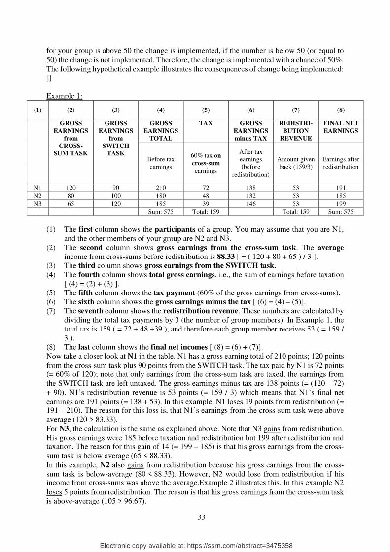
33

for your group is above 50 the change is implemented, if the number is below 50 (or equal to 50) the change is not implemented. Therefore, the change is implemented with a chance of 50%. The following hypothetical example illustrates the consequences of change being implemented: ]] Example 1:

(1) (2) (3) (4) (5) (6) (7) (8)

GROSS

EARNINGS

from CROSS-

SUM TASK

GROSS

EARNINGS

from SWITCH

TASK

GROSS

EARNINGS

TOTAL

TAX GROSS

EARNINGS

minus TAX

REDISTRI-

BUTION

REVENUE

FINAL NET

EARNINGS

Before tax earnings

60% tax on

cross-sum earnings

After tax earnings (before

redistribution)

Amount given back (159/3)

Earnings after redistribution

N1 120 90 210 72 138 53 191

N2 80 100 180 48 132 53 185

N3 65 120 185 39 146 53 199

Sum: 575 Total: 159 Total: 159 Sum: 575

(1) The first column shows the participants of a group. You may assume that you are N1,

and the other members of your group are N2 and N3. (2) The second column shows gross earnings from the cross-sum task. The average

income from cross-sums before redistribution is 88.33 [ = ( 120 + 80 + 65 ) / 3 ]. (3) The third column shows gross earnings from the SWITCH task. (4) The fourth column shows total gross earnings, i.e., the sum of earnings before taxation

[ (4) = (2) + (3) ]. (5) The fifth column shows the tax payment (60% of the gross earnings from cross-sums). (6) The sixth column shows the gross earnings minus the tax [ (6) = (4) – (5)]. (7) The seventh column shows the redistribution revenue. These numbers are calculated by

dividing the total tax payments by 3 (the number of group members). In Example 1, the total tax is 159 ( = 72 + 48 +39 ), and therefore each group member receives 53 ( = 159 / 3 ).

(8) The last column shows the final net incomes [ (8) = (6) + (7)]. Now take a closer look at N1 in the table. N1 has a gross earning total of 210 points; 120 points from the cross-sum task plus 90 points from the SWITCH task. The tax paid by N1 is 72 points (= 60% of 120); note that only earnings from the cross-sum task are taxed, the earnings from the SWITCH task are left untaxed. The gross earnings minus tax are 138 points (= (120 – 72) + 90). N1’s redistribution revenue is 53 points (= 159 / 3) which means that N1’s final net earnings are 191 points (= 138 + 53). In this example, N1 loses 19 points from redistribution (= 191 – 210). The reason for this loss is, that N1’s earnings from the cross-sum task were above average (120 > 83.33). For N3, the calculation is the same as explained above. Note that N3 gains from redistribution. His gross earnings were 185 before taxation and redistribution but 199 after redistribution and taxation. The reason for this gain of 14 (= 199 – 185) is that his gross earnings from the cross-sum task is below average (65 < 88.33). In this example, N2 also gains from redistribution because his gross earnings from the cross-sum task is below-average (80 < 88.33). However, N2 would lose from redistribution if his income from cross-sums was above the average.Example 2 illustrates this. In this example N2 loses 5 points from redistribution. The reason is that his gross earnings from the cross-sum task is above-average (105 > 96.67).


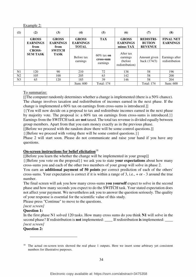
34

Example 2:

(1) (2) (3) (4) (5) (6) (7) (8)

GROSS

EARNINGS

from CROSS-

SUM TASK

GROSS

EARNINGS

from SWITCH

TASK

GROSS

EARNINGS

TOTAL

TAX GROSS

EARNINGS

minus TAX

REDISTRI-

BUTION

REVENUE

FINAL NET

EARNINGS

Before tax earnings

60% tax on

cross-sum earnings

After tax earnings (before

redistribution)

Amount given back (174/3)

Earnings after redistribution

N1 120 90 210 72 138 58 196

N2 105 100 205 63 142 58 200

N3 65 120 185 39 146 58 204

Sum: 600 Total: 174 Total: 174 Sum: 600

To summarize: [[The computer randomly determines whether a change is implemented (there is a 50% chance). The change involves taxation and redistribution of incomes earned in the next phase. If the change is implemented a 60% tax on earnings from cross-sums is introduced.]] {{You will now decide on a proposal to tax and redistribute incomes earned in the next phase by majority vote. The proposal is: a 60% tax on earnings from cross-sums is introduced.}} Earnings from the SWITCH task are not taxed. The total tax revenue is divided equally between group members. Apart from that you earn money exactly as in the previous phase. [[Before we proceed with the random draw there will be some control questions.]] {{Before we proceed with voting there will be some control questions.}}

Phase 2 will start soon. Please do not communicate and raise your hand if you have any questions. On-screen instructions for belief elicitation18

[[Before you learn the whether the change will be implemented in your group]] {{Before you vote on the proposal}} we ask you to state your expectations about how many cross-sums you and each of the other two members of your group will solve in phase 2. You earn an additional payment of 50 points per correct prediction of each of the others' cross-sums. Your expectation is correct if it is within a range of 3, i.e., + or - 3 around the true number. The final screen will ask you how many cross-sums you yourself expect to solve in the second phase and how many seconds you expect to do the SWITCH task. Your stated expectation does not affect your payment. We nevertheless ask you to answer the question seriously. The quality of your response is essential for the scientific value of this study. Please press "Continue" to move to the questions. [next screen]

Question 1: In the first phase N1 solved 120 tasks. How many cross sums do you think N1 will solve in the second phase? If redistribution is not implemented: ____ If redistribution is implemented: ____ [next screen]

Question 2:

18 The actual on-screen texts showed the real phase 1 outputs. Here we insert some arbitrary yet consistent numbers for illustrative purposes.


35

In the first phase N2 solved 80 tasks. How many cross sums do you think N2 will solve in the second phase? If redistribution is not implemented: ____ If redistribution is implemented: ____ [next screen]

Question 3.a: In the first phase you solved 65 tasks. How many cross sums do you think you will solve in the second phase? If redistribution is not implemented: ____ If redistribution is implemented: ____ Question 3.b: In the first phase you did the SWITCH task for 480 seconds. How many seconds do you think you will do the SWITCH task in the second phase? If redistribution is not implemented: ____ If redistribution is implemented: ____ [next screen]

Thank you for answering these questions. On the next screen, after all participants are done with their questions, [[you will learn whether the proposal is implemented in your group or not.]] {{you will vote on whether or not to implement the proposal in your group.}} {{[next screen]

If your expectations are correct your earnings in phase 2 will be: If redistribution is not implemented: 185 If redistribution is implemented: 199 I am voting for the proposal: Yes, No}} [next screen]

[[The number from the random draw for your group is: x The change is NOT / IS

implemented.]] {{The result of the vote is: The proposal IS / is NOT accepted}}


36

Appendix A2: Descriptive statistics

Appendix A2 provides descriptive statistics on the number of cross sums solved, the time spent

on solving cross sums and the monetary total profit obtained from the experiment.

Table A2.1: Descriptive statistics sorted by treatment

Treatment Output Work time Profit

Phase 1 Mean Median Mean Median Mean Median

EndoNoR ExoNoR Total NR (n = 150) EndoR ExoR Total R (n = 90)

105.9 105.5 105.8

103.9 108.3 105.2

108 105 108

105 111 107

850.2 783.4 835.5

880.2 825.2 863.7

909.8 766.1 907.5

999.4 905.3 978.1

127.6 131.4 128.4

124.0 132.1 126.5

126 126 126

123 132 126

Phase 2

EndoNoR ExoNoR Total NR (n = 150) EndoR ExoR Total R (n = 90)

107.4 114.5 108.9

92.9 82.9 89.9

105 114 105

99 93 96

832.4 878.3 842.5

702.4 514.6 646.1

843.6 897.4 857.1

765.5 505.8 638.7

130.7 135.0 131.6

124.3 127.1 125.2

130 133 130

122 128 126

Note: Duration of each phase is 1200 seconds. Work time is calculated as 1200 – leisure time in phase x with x ϵ {1, 2}. Profits are calculated as the sum of earnings from cross-sum task, “Switch task” and transfers as explained in Section 2. The samples of the different treatment groups can be assumed to stem from the same population (p = 0.967, Kruskal-Wallis-test).

Appendix A3: Disincentive effect – some theoretical insights

Appendix A3 summarizes as to why we expect a disincentive effect from redistribution to be

present in our design.

Consider an economic agent who chooses to allocated a time budget A to work + or leisure

A � +. Agent i’s production function B��+� shows how much output (i.e., how many cross

sums) are produced when solving cross sums for +� seconds, with B�C > 0, B�CC < 0. A unit of

time allocated to leisure yields a constant return F. Work is rewarded at a constant piece rate G.

Absent taxation and redistribution individual profit is:

H� � GB��+� + F�Z � +� (A3.1)

Maximizing (A3.1) with respect to working time J� yields the optimality condition for J�∗

(in condition NoR)

B�C�+� � KL (A3.2)


37

Thus, the profit-maximizing choice is to work in the real-effort task up to the point where

the marginal return of solving one cross sum equals its marginal (opportunity) costs. Since more

productive individuals have marginal productivity BC above less productive individuals at any

+, they find it optimal to work longer than less productive workers.

With a tax of ! on labor income and per capita redistribution to � agents in a group, profits

are:

H� � �1 � !GB��+� + F�A � +� + MNG ∑ BPQ+PR�PS� (A3.3)

Maximizing (A3.3) with respect to +� yields the optimality condition for +�∗ (in condition

R):

B�C�+� � KLQM

NTUVMR � KLW (A3.4)

Since G� < G, it follows that redistribution causes a disincentive effect (with our specific

parameters, G� � 0.6. The disincentive effect results from substituting work for labor because

the relative price of work increases. Figure A3.1 illustrates the disincentive effect.

Eq. A3.4 shows that the magnitude of the disincentive effect depend on the shape of the

production function. While the disincentive effect is larger for more productive than for less

productive agents in absolute terms, they can be smaller or equal in relative terms. For example,

with B��+ � F��+�, the relative disincentive effect is independent of productivity.

If subjects participating in our experiment are strictly self-interested, and absent of

selection, we should not observe any differences in subjects’ average reactions to redistribution

between the Endo and Exo treatments.


38

Figure A3.1: Illustration of disincentive effect from redistribution

The disincentive effect results in reduced aggregate profits:

∑ HP�PS� � �1 � !G ∑ BPQ+PR�PS� + FQ�A � ∑ +P�PS� R + !G ∑ BPQ+PR�PS� (A3.5)

Maximizing (A3.5) with respect to +� again yields B��+� � F/G as in the case without

distribution. The reason is that redistribution is not costly per se.

We find that more productive workers have a stronger disincentive effect than less

productive workers. We classify workers as ‘more productive’ who have outputs above the

median in phase 1, and those below the median as ‘less productive’. The disincentive effect for

less productive workers is -3.0% while it is much stronger (-27.0%) for high productive workers

(pooled data for EndoR and ExoR). The finding on heterogeneous disincentive effects with

respect to productivity is mirrored in the data for time spent working. More productive workers

reduce time spent working by 38.9% while the less productive workers reduce it by 13.6% on

average.19

19 The difference in output and time spent on the task are statistically significant at the 1% level (p < 0.01, z-test). Since more and less productive individuals may be members of the same group, we cannot employ the usual non-parametric tests in this case. Thus, we conducted a regression analysis testing for differences in intercepts using robust standard errors for intra-group correlations.


39

Appendix A4: Disincentive effect in EndoR by voting

Figure A4.1 displays a more detailed version of Figure 5 that additionally holds information on

how subjects voted. Figure A4.1 shows that selection via voting cannot explain the observed

difference in output change. In fact, there is no difference between yes- and no-voters in terms

of change of output from phase 1 to 2 (p = 0.142 and p = 0.432 in NoR and R, respectively,

two-sided Fisher’s exact test).

Figure A4.1: Disincentive effect with endogenous redistribution (Endo)


�� 1.51 n(no) = 83, n(yes) = 34

With redistribution

�� 10.95 n(no) = 20, n(yes) = 43

Notes: Each dot represents data from one subject. The dashed 45° line denotes equal output in phase 1 and 2. In contrast to ExoR (see right panel of Figure 4), the disincentive effect is much less pronounced in EndoR.

Appendix A5: A measure of deviation from optimal stopping time

Appendix A5 defines the metric used to capture the central variable of overtime.

A screen has 3 tasks. Optimizing subjects should not take longer than 15’’ (9’’) per task

w/o (with) redistribution. Call S_1 the last screen before a subject takes more than this

maximum time. Call S_N the last screen before a subject stops working. The deviation from

the optimal stopping time is calculated as the average time needed for a task on the screens

{S_1, S_2, S_3, … , S_N} minus 15’’ (9’’ in case of redistribution). Note: Some subjects stop

04

080

12

016

0

Nu

mb

er

of

tasks in

pha

se 2

0 40 80 120 160


No voters Yes voters 45° line

04

080

12

016

0

Nu

mb

er

of

tasks in

pha

se 2

0 40 80 120 160


No voters Yes voters 45° line


40

working before they ever used 15’ (9’) per task w/o (with) redistribution. In this case, S_1 =

S_N.

Figure A5.1 shows the time per screen on the y-axis and the cumulated number of solved

screens on the x-axis for an example subject. Our measure Deviation from optimal stopping

time considers the sum of (positive and negative) deviation from 45’ (divided by 3), over S_1

to S_N (S.dev = 29.4, min. = -103.0’’, max. 86.9’’).

Figure A5.1: Illustration of the measure of deviating from optimal stopping time

Appendix A6: Regression results conditional on voting

Tables A6.1 and A6.2 replicate the regression analysis conducted in Table 1 of the paper, but

split by voting behavior.

02

040

60

80

Tim

e n

ee

ded

pe

r scre

en

(3

cro

ss s

um

s)

0 50 100 150

Number of cross sums completed

S_1

S_N


41

Table A6.1: Regression analysis (No-voters only)

(1) (2) (3) (4) Output Worktime Productivitya) Overtimeb)

Treatment EXO

(i) constant 105.45*** 783.36*** 215.76*** -10.47** (5.12) (52.83) (6.34) (5.26) (ii) phase 9.09* 94.97* 4.85 3.94 (4.81) (54.55) (6.74) (6.47) (iii) redistribution 2.88 41.82 -0.94 2.61 (7.63) (78.75) (9.45) (7.84) (iv) phase x redistribution -34.54*** -405.54*** -22.26** 13.41 (7.16) (81.32) (10.05) (9.64)


Treatment ENDO

(v) constant 119.46*** 955.88*** 218.75*** -7.75** (3.64) (30.22) (4.81) (3.28) (vi) phase -1.66 -60.92** 6.27** 0.33 (2.19) (28.68) (2.47) (3.68) (vii) redistribution -3.81 26.68 -10.25 2.43 (7.32) (64.69) (10.00) (7.26) (viii) phase x redistribution -12.89*** -185.12*** -6.27 32.02*** (4.97) (65.08) (5.60) (8.36)



(i)-(v) const -13.79** -172.00*** -3.25 -2.73 (6.43) (57.08) (10.07) (6.22) (ii)-(vi) phase 10.75** 155.89*** -1.42 3.61 (4.75) (57.95) (9.33) (7.19) (iii)-(vii) redistribution 6.47 14.63 9.56 0.19 (10.93) (99.37) (16.46) (10.73) (iv)-(viii) phase x redistribution -21.65*** -220.41** -15.99 -18.60 (8.30) (101.29) (16.32) (12.56)


Notes: All columns show coefficients of linear multi-level regressions (with hierarchical error clustering: subjects nested in groups); standard errors in parentheses; levels of significance: * p < 0.1, ** p < 0.05, *** p < 0.01. The diff-in-diff-in-diff model for productivity did not converge with the hierarchical error specification; therefore, we provide estimates based on a simpler model with group level error clustering only. a) Productivity is measured as number of completed tasks per second within the first five minutes of a phase (coefficients are multiplied by 1000 for better visibility). b) Overtime is defined as the difference between actual and optimal stopping time, averaged across all observations as from just before the optimal stopping time was exceeded for the first time. For more details and a graphical example see Appendix A5.


42

Table A6.2: Regression analysis (Yes-voters only)

(1) (2) (3) (4) Output Worktime Productivitya) Overtimeb)

Treatment EXO

(i) constant 105.45*** 783.36*** 215.76*** -10.47** (5.12) (52.83) (6.34) (5.26) (ii) phase 9.09* 94.97* 4.85 3.94 (4.81) (54.55) (6.74) (6.47) (iii) redistribution 2.88 41.82 -0.94 2.61 (7.63) (78.75) (9.45) (7.84) (iv) phase x redistribution -34.54*** -405.54*** -22.26** 13.41 (7.16) (81.32) (10.05) (9.64)


Treatment ENDO

(v) constant 73.59*** 593.78*** 171.18*** 5.06 (4.70) (60.97) (6.07) (6.15) (vi) phase 9.26 87.29 12.06** 2.71 (5.65) (74.88) (5.37) (7.15) (vii) redistribution 24.78*** 238.80*** 23.49*** -1.16 (6.29) (81.59) (8.44) (8.23) (viii) phase x redistribution -18.54** -233.35** -11.13 39.86*** (7.56) (100.20) (7.19) (9.57)



(i)-(v) const 31.87*** 189.58** 44.58*** -15.53* (6.92) (81.55) (8.74) (8.08) (ii)-(vi) phase -0.17 7.69 -7.21 1.23 (7.51) (94.69) (8.49) (9.72) (iii)-(vii) redistribution -21.91** -196.98* -24.18* 3.77 (9.81) (115.61) (12.40) (11.45) (iv)-(viii) phase x redistribution -15.99 -172.18 -11.13 -26.45* (10.64) (134.24) (12.04) (13.78)


Notes: All columns show coefficients of linear multi-level regressions (with hierarchical error clustering: subjects nested in groups); standard errors in parentheses; levels of significance: * p < 0.1, ** p < 0.05, *** p < 0.01. For definitions of a) and b) see notes of Table A6.1. For more details and a graphical example see Appendix A5.


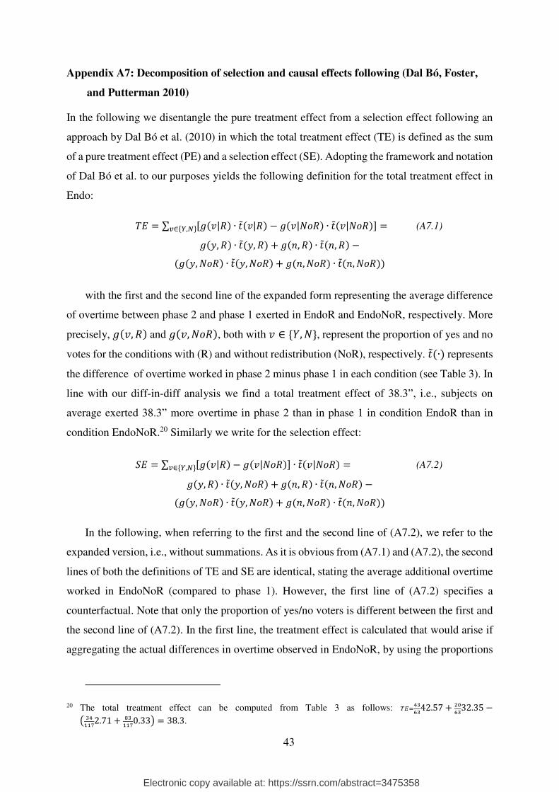
43

Appendix A7: Decomposition of selection and causal effects following (Dal Bó, Foster,

and Putterman 2010)

In the following we disentangle the pure treatment effect from a selection effect following an

approach by Dal Bó et al. (2010) in which the total treatment effect (TE) is defined as the sum

of a pure treatment effect (PE) and a selection effect (SE). Adopting the framework and notation

of Dal Bó et al. to our purposes yields the following definition for the total treatment effect in

Endo:

+, � ∑ XY��|[ ∙ !̃��|[ � Y��|^_[ ∙ !̃��|^_[`(∈b*,�c � (A7.1)

Y�d, [ ∙ !̃�d, [ + Y��, [ ∙ !̃��, [ �

�Y�d, ^_[ ∙ !̃�d, ^_[ + Y��, ^_[ ∙ !̃��, ^_[

with the first and the second line of the expanded form representing the average difference

of overtime between phase 2 and phase 1 exerted in EndoR and EndoNoR, respectively. More

precisely, Y��, [ and Y��, ^_[, both with � ∈ be, ^c, represent the proportion of yes and no

votes for the conditions with (R) and without redistribution (NoR), respectively. !̃�∙ represents

the difference of overtime worked in phase 2 minus phase 1 in each condition (see Table 3). In

line with our diff-in-diff analysis we find a total treatment effect of 38.3”, i.e., subjects on

average exerted 38.3” more overtime in phase 2 than in phase 1 in condition EndoR than in

condition EndoNoR.20 Similarly we write for the selection effect:

-, � ∑ XY��|[ � Y��|^_[` ∙ !̃��|^_[ �(∈b*,�c (A7.2)

Y�d, [ ∙ !̃�d, ^_[ + Y��, [ ∙ !̃��, ^_[ �

�Y�d, ^_[ ∙ !̃�d, ^_[ + Y��, ^_[ ∙ !̃��, ^_[

In the following, when referring to the first and the second line of (A7.2), we refer to the

expanded version, i.e., without summations. As it is obvious from (A7.1) and (A7.2), the second

lines of both the definitions of TE and SE are identical, stating the average additional overtime

worked in EndoNoR (compared to phase 1). However, the first line of (A7.2) specifies a

counterfactual. Note that only the proportion of yes/no voters is different between the first and

the second line of (A7.2). In the first line, the treatment effect is calculated that would arise if

aggregating the actual differences in overtime observed in EndoNoR, by using the proportions

20 The total treatment effect can be computed from Table 3 as follows: f�S567642.57 + 89

7632.35 �Q 65

UUg2.71 + h6UUg0.33R � 38.3.


44

of yes/no voters, as they occurred in EndoR. If there was no selection effect, the first line should

be equal in size to the second line of (A7.2) and, thus, -, � 0. The question for identifying the

selection effect is “How much additional overtime do we expect subjects to have worked in

EndoR, not because of whether redistribution was implemented, but because of a different

proportion of yes/no votes?” In other words, the selection effect is caused by the change in

voting behavior, conditional on whether redistribution was implemented.21 Applying this

approach to our data we can calculate a selection effect of 0.93”, i.e., in our experiment, a total

of 0.93” out of 38.2” of additionally exerted overtime in phase 2 can be attributed to selection

rather than redistribution.22 Complementarily, the pure treatment effect (PE) is defined as the

residual of the total treatment effect that is not explained by selection:

i, � +, � -, � ∑ Y��|[ ∙ X!̃��|[ � !̃��|^_[`(∈b*,�c � (A7.3)

Y�d, [ ∙ !̃�d, [ + Y��, [ ∙ !̃��, [ �

QY�d, [ ∙ !̃�d, ^_[ + Y��, [ ∙ !̃��, ^_[R

Given our data, we find a pure treatment effect of 37.4”.23

Appendix A8: No selection on observables

No selection of non-optimizing subjects into R.

A possible selection account would be that some subjects succeed in optimizing (stop working

optimally) and vote against redistribution. Others fail to stop optimally (thus work too long)

and vote for redistribution. Hence, subjects who work excessively long tend to sort into

redistribution. A related but alternative story is that subjects who respond optimally to changes

in incentives vote against redistribution while those who underreact to the change in relative

prices vote for redistribution. We provide the following tests for such stories. By splitting the

sample by the median of overtime, we sort subjects into those who on average exert more

overtime in phase 1 (n = 93) and those who exert less or no overtime (n = 87). We find that the

non-optimizing subjects in phase 1 (in terms of exerting more overtime than others) are not

more likely to vote yes (p = 0.548, two-sided Fisher’s exact test). In addition, we find that the

21 In the words of Dal Bó et al. (2010, p.2218, square brackets added): “The selection effect captures the changes in cooperation [i.e., overtime in our case] that arise not from the change in treatment [i.e., R or NoR] but from the change in the proportion of types of subjects [i.e., proportion of yes or no votes].”

22 From Table 3: -, � 56762.71 + 89

760.33 � Q 65UUg2.71 + h6

UUg0.33R � 0.93.

23 From Table 3: i, � 567642.57 + 89

7632.35 � Q56762.71 + 89

760.33R � 37.4.


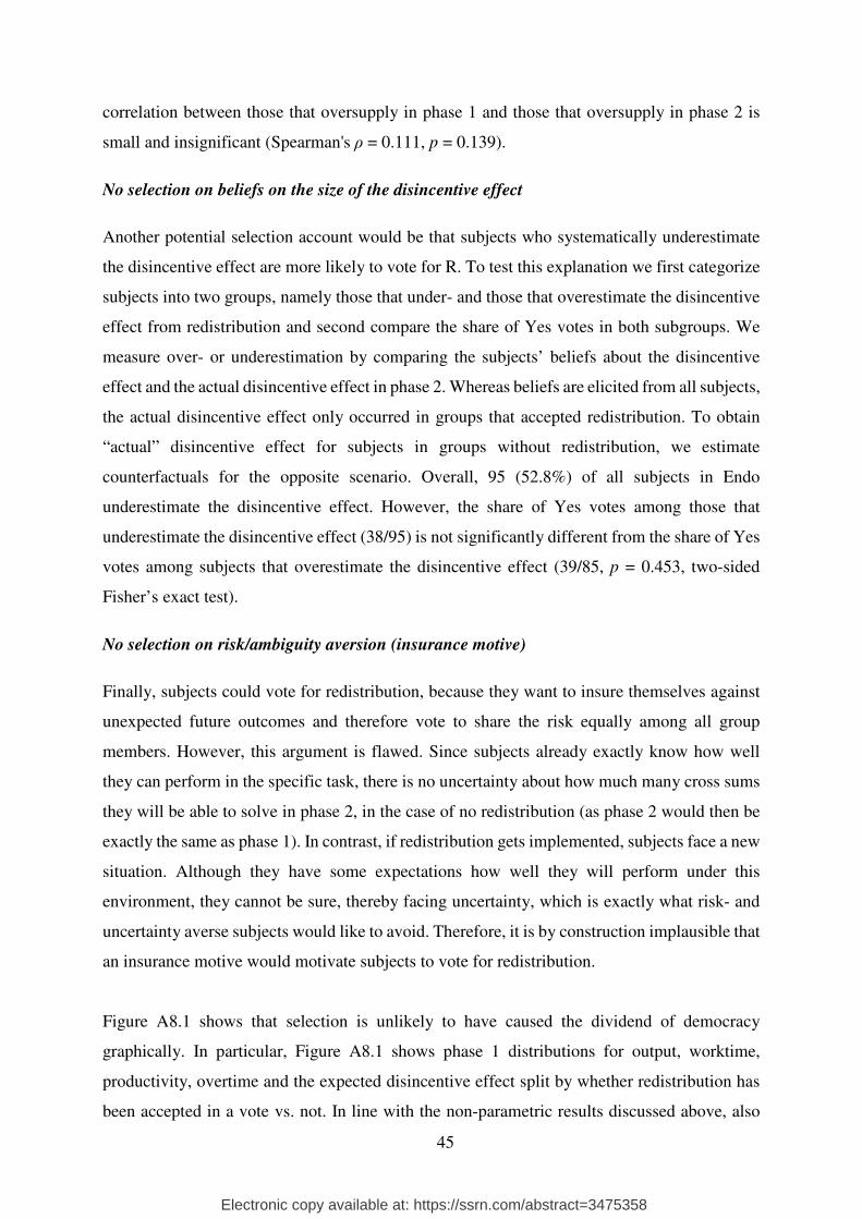
45

correlation between those that oversupply in phase 1 and those that oversupply in phase 2 is

small and insignificant (Spearman's ρ = 0.111, p = 0.139).

No selection on beliefs on the size of the disincentive effect

Another potential selection account would be that subjects who systematically underestimate

the disincentive effect are more likely to vote for R. To test this explanation we first categorize

subjects into two groups, namely those that under- and those that overestimate the disincentive

effect from redistribution and second compare the share of Yes votes in both subgroups. We

measure over- or underestimation by comparing the subjects’ beliefs about the disincentive

effect and the actual disincentive effect in phase 2. Whereas beliefs are elicited from all subjects,

the actual disincentive effect only occurred in groups that accepted redistribution. To obtain

“actual” disincentive effect for subjects in groups without redistribution, we estimate

counterfactuals for the opposite scenario. Overall, 95 (52.8%) of all subjects in Endo

underestimate the disincentive effect. However, the share of Yes votes among those that

underestimate the disincentive effect (38/95) is not significantly different from the share of Yes

votes among subjects that overestimate the disincentive effect (39/85, p = 0.453, two-sided

Fisher’s exact test).

No selection on risk/ambiguity aversion (insurance motive)

Finally, subjects could vote for redistribution, because they want to insure themselves against

unexpected future outcomes and therefore vote to share the risk equally among all group

members. However, this argument is flawed. Since subjects already exactly know how well

they can perform in the specific task, there is no uncertainty about how much many cross sums

they will be able to solve in phase 2, in the case of no redistribution (as phase 2 would then be

exactly the same as phase 1). In contrast, if redistribution gets implemented, subjects face a new

situation. Although they have some expectations how well they will perform under this

environment, they cannot be sure, thereby facing uncertainty, which is exactly what risk- and

uncertainty averse subjects would like to avoid. Therefore, it is by construction implausible that

an insurance motive would motivate subjects to vote for redistribution.

Figure A8.1 shows that selection is unlikely to have caused the dividend of democracy

graphically. In particular, Figure A8.1 shows phase 1 distributions for output, worktime,

productivity, overtime and the expected disincentive effect split by whether redistribution has

been accepted in a vote vs. not. In line with the non-parametric results discussed above, also


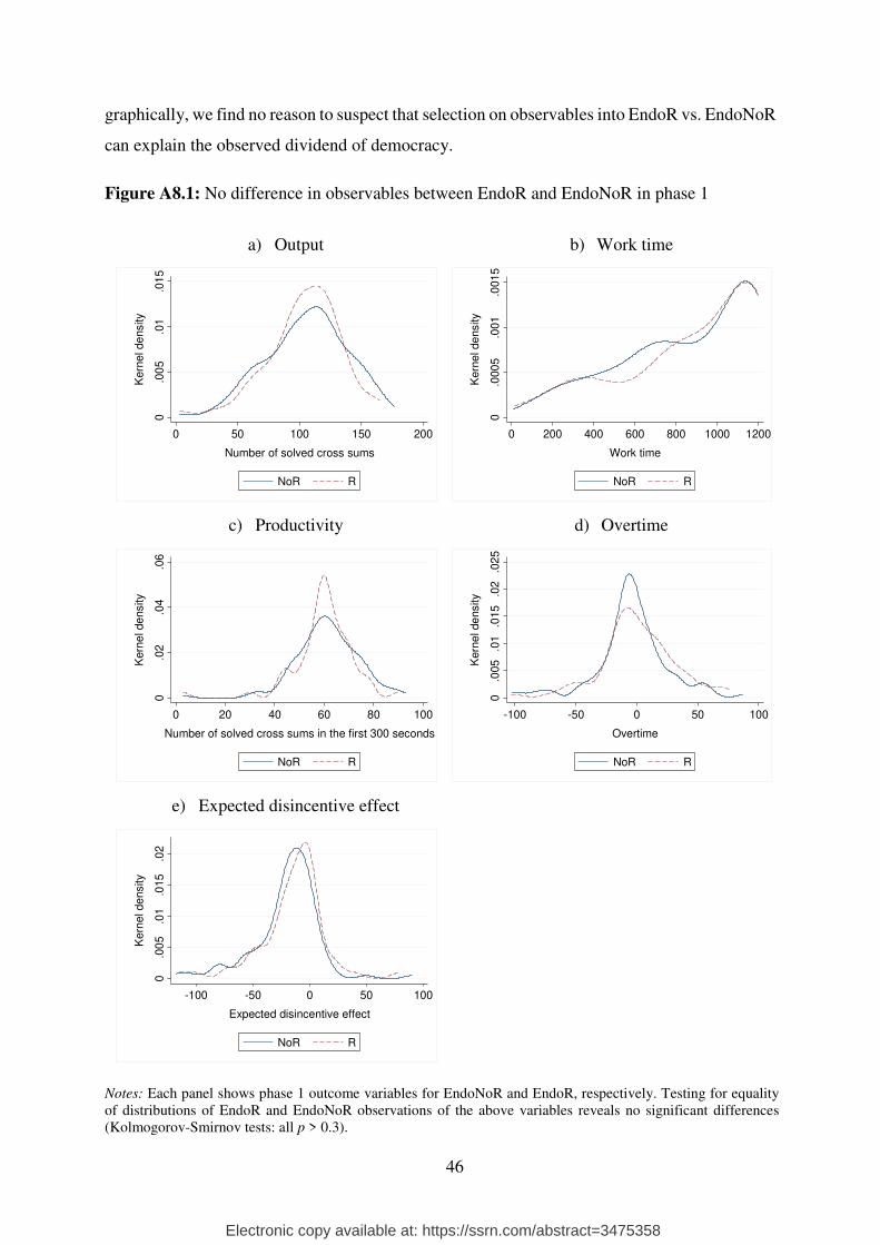
46

graphically, we find no reason to suspect that selection on observables into EndoR vs. EndoNoR

can explain the observed dividend of democracy.

Figure A8.1: No difference in observables between EndoR and EndoNoR in phase 1

a) Output b) Work time

c) Productivity d) Overtime

e) Expected disincentive effect

Notes: Each panel shows phase 1 outcome variables for EndoNoR and EndoR, respectively. Testing for equality of distributions of EndoR and EndoNoR observations of the above variables reveals no significant differences (Kolmogorov-Smirnov tests: all p > 0.3).

0.0

05

.01

.01

5

Kern

el de

nsity

0 50 100 150 200

Number of solved cross sums

NoR R0

.000

5.0

01

.001

5

Kern

el de

nsity

0 200 400 600 800 1000 1200

Work time

NoR R

0.0

2.0

4.0

6

Kern

el de

nsity

0 20 40 60 80 100

Number of solved cross sums in the first 300 seconds

NoR R

0.0

05

.01

.015

.02

.02

5

Kern

el de

nsity

-100 -50 0 50 100

Overtime

NoR R

0.0

05

.01

.015

.02

Kern

el de

nsity

-100 -50 0 50 100

Expected disincentive effect

NoR R


47

Appendix A9: Ruling out alternative explanations for the “dividend of democracy”

Conditional cooperation based on production beliefs

Tyran and Feld (2006) find that their results are driven by commitment and conditional

cooperation. To check whether conditional cooperation drives our results, we investigate the

expectations stated by participants and find that conditional cooperation cannot explain the

dividend of democracy.

Figure A9.1: Stated expectations concerning own output change and the average output change of the other two group-members under the scenario of implemented redistribution

Endogenous redistibution Yes-Voters No-Voters

Exogenous redistribution

Notes: The top panels and the bottom panel contain observations from the scenario of endogenous and exogenous redistribution only, respectively; the dashed line represents equal output.

In particular, we check whether people with higher output expectations for themselves in

phase 2 also expect higher output by the other group members. Such a pattern would be

consistent with conditional cooperation. Figure A9.1 shows the results for the expectations

concerning own output change as well as the average output change of the other group-members

-15

0-1

00

-50

05

0100

Expecte

d o

wn o

utp

ut chang

e

-150 -100 -50 0 50 100Average expected output change of others

-15

0-1

00

-50

05

0100

Expecte

d o

wn o

utp

ut chang

e


-15

0-1

00

-50

05

0100

Expecte

d o

wn o

utp

ut chang

e


n = 77 n = 103

n = 60


48

for the scenario of implemented redistribution. The graph in the top left panel contains

information stated by yes-voters (Endo), while the top right graph illustrates the expectations

disclosed by no-voters (Endo). Subject expecting that the other two group members will reduce

their production because of redistribution in phase 2 by a lot, tend also to expect their own

production to decrease substantially. This regularity is strong, independent of how the subject

voted (Spearman ρ = 0.399, p = 0.003 for yes-voters and ρ = 0.577, p < 0.001 for no-voters).

These results are consistent with the interpretation that a substantial fraction of subjects in Endo

are conditional cooperators, but independent of their actual voting behavior.

The finding that no-voters increase their labor supply in phase 2 can be classified as being

irrational, with respect to a Nash-solution. This suggests that voting induces a signaling effect.

Taking into consideration that no-voters tend to be conditional cooperators, as is shown in

Figure A9.1, such a signaling effect could result in a social norm to cooperate. The fact that no-

voters in EndoR expect to react more strongly to a redistributive tax system than yes-voters (p

= 0.032, z-test), but subsequently substantially over-provide work effort (in terms of overtime,

p < 0.001, z-test), corroborates this hypothesis. However, since the stated expectations of

subjects in ExoR show a highly significant correlation of own and other output change as well

(see Figure A9.1 bottom panel, ρ = 0.461, p < 0.001), the existence of conditional cooperators

in the population alone cannot explain the observed endogeneity premium.

Inequality aversion

This potential explanation is based on the notion that more productive voluntarily work more

(beyond their rational stopping time) to support the less productive, whereas the less productive

should stop at their rational stopping time. Any overtime would further reduce their payoff and

therefore their utility, particularly so when taking into account the higher payoffs of the more

productive group members. We find that inequality aversion does not explain the dividend of

democracy in our data.

To test whether inequality aversion could explain our results, we investigate the behavior

of the most and the least productive subject of a group. Did the most productive subjects

increase their production beyond their rational stopping time? In fact, the most productive

subjects on average worked 35 seconds longer than optimal under EndoR in phase 2. This

represents a substantial increase in overtime (diff = 34.55 seconds) since in phase 1, most

productive subjects only worked 0.61 seconds longer than optimal. However, the least

productive subjects do not behave differently. Whereas on average working 5.29 seconds less

than optimal in phase 1, they work 31.01 seconds overtime in phase 2 (diff = 36.30 seconds).


49

Most and least productive subjects do not show significantly different behavior, neither in phase

1 nor in phase 2 (all p > 0.1, WRS; diff-in-diff: p = 0.403), suggesting that also the least

productive subjects exerted significant amounts of costly overwork, making it highly

implausibly that subjects were motivated by inequality aversion. In that sense our finding is in

line with Buch and Engel (2012) who also investigate such inequality effects, but do not find

empirical support.

Reciprocating to “kind” (unselfish) voting behavior of more productive group members

We find no evidence for positive reciprocity driving the dividend of democracy. Whereas for

less productive subjects it is in their best monetary interest to vote for redistribution, also a

substantial number of more productive subjects voted yes. As discussed above, one potential

reason for this could be inequality aversion.24 However, this specific social preference cannot

explain why both less and more productive indistinguishably from one another work much

longer in EndoR, since any overtime worked by the less productive will reduce their income

and therefore increase inequality.

A more plausible explanation for excessive overtime in phase 2 under EndoR, particularly

for the less productive, seems to be conditionally cooperative behavior. Since all group

members know their own and the others’ output of phase 1, they have a good understanding of

whether they and the other group members would benefit from redistribution in phase 2 (see

Table 2). Consequently, if a less productive subject observes that the group accepted

redistribution, he/she could interpret this as a signal of kindness (since the other group members

most likely sacrificed their own income by voting yes). This interpretation could induce a

willingness to reciprocate, i.e., make less productive subjects over-exert effort beyond their

rational stopping point to compensate the other group members for their selfless voting

decision.

Along these lines, if conditional cooperation was the main motive for overtime, more

productive workers would not need to work longer than rational in phase 2 since they already

did their part by working hard in phase 1 and by voting for redistribution. That is, in phase 2,

24 From Table 2 we know that in total 23 subjects who held correct expectations voted for redistribution although this was against their monetary interests. Whereas inequality aversion could be a motive for voting yes that is present in both less and more productive subjects, because of the perfect correlation in the prediction of inequality averse and self-interested behavior for the less productive, we cannot say to what extent inequality aversion might have played a role for the less productive.


50

we should find considerable overtime by the less productive group members and much less

overtime by more productive individuals. However, this is not what we observe.

Figure A9.2: Change in overtime in Endo, by phase 1 output and redistribution

Figure A9.2 illustrates the change of overtime between phase 1 and 2, for the least, the

median and the most productive subjects per group, separately. Clearly, there is only a tiny (1.7

second), non-significant difference between the overtime worked by subjects with low and high

productivity, respectively (p = 0.888, z-test), which does not fit a narrow tit-for-tat conditional

cooperation type of explanation.

Appendix A10: Welfare effects of redistribution

In our experiment, subjects could earn income from labor (which could be taxed) and leisure

(which never was taxed). While in section 3 of the article, we provide evidence for a strong

disincentive effect on labor incomes, we now also demonstrate that redistributions also reduced

overall incomes (including untaxed income from leisure).

The direct cost of less income from work is partially counter-balanced by the gain in

income from increased leisure. Nevertheless, in Exo, average overall income, including income

from leisure, falls by about 6.5% (� ��H, �� 3.58 � . �� 4.96, p = 0.004,

WRS). That is, imposed redistribution did not only significantly reduce labor income but also

significantly reduced overall income. In contrast, in Endo, labor income falls less and overall

income, i.e., including income from leisure, even is marginally significantly higher with

democratic redistribution (��H � �2.85 � . ��H � �8.54, p = 0.034, z-test).

-20

020

40

60

Cha

nge

in o

ve

rtim

e (

phase 2

- p

hase

1)

NoR R

low middle high low middle high


51

Appendix A11: Visual representation of differential disincentive effects

Figure A11.1 shows that redistribution causes a substantial disincentive effect in worktime. In

particular, in Endo, the average change in worktime from phase 1 to phase 2 under redistribution

is -177.80 seconds and is significantly larger than under NoR (-17.85 seconds, ranksum test, p

= 0.001). In Exo, the average change in worktime is also significantly different between R and

NoR (R: -310.56 vs. NoR: 94.97 seconds, ranksum test, p = 0.004). Visually, these different

changes in worktime between R and NoR conditions are indicated by a downward shift of the

observations from the left to the right panels of Figure A11.1.

Furthermore, a steeper slope of the linear fit indicates that more productive workers reduce

their worktime by a larger extent than less productive workers (z-test for equality of slopes

between NoR vs. R, p < 0.001) and that this effect is much more pronounced under imposed

than under chosen redistribution (p = 0.010, z-test for equality of slopes EndoR vs. ExoR).

Figure A11.1: Change in work time in seconds by number of cross sums solved in phase 1

Notes: The slopes in both NoR conditions are very similar (left panels, p = 0.855, z-test for equality of slopes), whereas the decrease in working time when redistribution is introduced in phase 2 is clearly stronger in ExoR (bottom right), than in EndoR (top right, p = 0.010, z-test for equality of slopes).

-10

-50

51

0-1

0-5

05

10

0 50 100 150 200 0 50 100 150 200

Endo, NoR Endo, R

Exo, NoR Exo, R

Change in h

undre

d o

f seconds

Number of completed cross sums in phase 1


Documents

Disincentives from Redistribution: Evidence on a Dividend