Embed Size (px)
Citation preview

Discussion Papers in Economics
Department of Economics and Related Studies
University of York
Heslington
York, YO10 5DD
No. 14/22
Who is afraid of austerity? The redistributive
impact of fiscal policy in a DSGE framework
Richard McManus, F. Gulcin Ozkan and Dawid
Trzeciakiewicz


Who is afraid of austerity? The redistributive impactof fiscal policy in a DSGE framework∗
Richard McManusUniversity of York
F. Gulcin Ozkan†
University of YorkDawid Trzeciakiewicz
University of Birmingham
21 July 2014
Abstract
This paper presents a comprehensive assessment of fiscal austerity, with special
emphasis on its distributional consequences, which are surprisingly ignored in the
existing literature. Using a medium scale DSGE model we find that both the
aggregate and distributional consequences of fiscal consolidation are shaped by its
composition much more than by its speed. A trade-off emerges between efficiency
and equality; spending-based austerity leads to smaller net movements in output,
incomes and welfare, but also to larger inequality between agents who vary by their
access and use of credit markets. Given the severity of the recent downturn in most
advanced economies that had adopted austerity, this trade-off between growth and
distributional consequences of fiscal consolidation is likely to pose serious challenges
to policymakers in many countries.
Keywords: fiscal austerity; welfare; redistribution.
JEL Classification: E65; H2; H3.
∗Comments from the participants at The European Monetary Forum workshop at the University ofGlasgow, 8-9 March 2013; MMF Annual Conference at Queen Mary College, 11-13 September 2013 andthe Royal Economic Society Annual Conference at the University of Manchester, 7-9 April, 2014 aregratefully acknowledged.†Corresponding author. Department of Economics and Related Studies (DERS), University of York,
Heslington, York, YO10 5DD, UK; Tel: 01904-434673; E-mail:[email protected].
1

1 Introduction
There has been a great revival of interest in fiscal policy issues in both policy and academic
circles following the 2008-09 global financial crisis. Substantial fiscal stimulus packages
that were put in place in response to the crisis were followed by much reduced fiscal
revenues during the subsequent Great Recession, leading to a clear loss of fiscal discipline,
particularly in advanced economies.1 For example, debt to GDP ratios reached an average
of 92.3 per cent in OECD countries with 89 per cent in the UK, 99 per cent in the US,
126 per cent in Italy and 210 per cent in Japan in 2009 (see, for example, OECD; 2012).
Such fiscal sustainability issues that surfaced soon after the adoption of the large
fiscal stimulus packages have forced widespread policy reversals. The resulting fiscal
consolidation has proved difficult both politically and economically in many countries.
Challenges fiscal austerity posed for different sections of the society have been at the top of
the political agenda in both the US and the UK since 2010, for example. A key question
related to fiscal adjustment is therefore, how the cost of consolidation is distributed.
Although the effectiveness of fiscal programs, both stimulus and consolidation, is widely
explored in existing work, the distributional impact of fiscal policy is largely ignored.2
This is somewhat surprising given the clear distributional implications of fiscal austerity,
as is evident from the recent policy discussions.3
It is also widely acknowledged that austerity programs that are viewed as ‘unfair’ are
unlikely to succeed (see, for example, IMF; 2012). Agnello et al. (2012) and IMF (2012)
1The fiscal stimulus programmes were as large as 5.9 per cent of GDP in the US, 3.3 per cent onaverage in OECD and 4.8 per cent in China in 2008 among many others (see, for example, OECD; 2009).
2Due to the the sharp contraction in global economic activity since 2008, recent work has primarilyfocussed on the output implications of fiscal policy and thus on the size of fiscal multipliers identifyinga wide range of values: varying from 1.6 (Romer and Bernstein; 2009) to much smaller figures that areclose to zero (Cogan et al.; 2010).
3To the best of our knowledge there are two exceptions to this: Drautzburg and Uhlig (2011) andMcManus (2012). The former finds that the specific policy of the American Recovery and ReinvestmentAct was detrimental to all agents over the lifetime of the policy unless the future is discounted atunfeasibly high rates. Positive impacts of the policy are the main focus of the paper, however, andthe normative impacts are not fully considered. The latter finds that counter-cyclical policy, especiallythose targeting government spending, is to the benefit of credit-constrained agents and the detrimentto the unconstrained. However, in contrast to our paper, the latter excludes many empirically relevantinstruments within the framework of a smaller model.
2

present empirical evidence suggesting that periods of fiscal consolidation are associated
with increases in income inequality. Moreover, Granados (2005) find that the composition
of consolidations play a key role on their consequences for income inequality. Indeed,
Woo et al. (2013) show that spending-based consolidations tend to worsen inequality
more significantly, as compared with tax-based consolidations.
This paper explores both the aggregate and distributional impact of fiscal austerity
by utilizing a dynamic stochastic general equilibrium model (DSGE) with real and nom-
inal frictions. To that end, our framework incorporates heterogeneity of agents regarding
access to credit into a medium scale New Keynesian DSGE model. Ricardian consumers
own the entire capital stock of the economy and possess access to the financial mar-
kets, that are assumed to be complete. Non-Ricardian households, on the other hand,
simply consume their total disposable income arising from labour and transfers. Firms
produce differentiated goods, choose labour and capital inputs and set prices similar to
the method proposed by Calvo (1983). The monetary authority sets the nominal interest
rate according to a Taylor rule. The fiscal authority has a set of policy instruments at
its disposal with which to respond to the cyclical changes in debt.
This paper makes two distinct contributions. The first is to combine a comprehensive
examination of the distributive consequences of fiscal austerity, which has received very
little attention in the existing literature, with one which focuses on other macroeconomic
outcomes. Our distributional analysis has two dimensions: welfare and income distribu-
tion. We examine the normative implications of different fiscal packages for both types
of households, and as such shed light on the ranking of policies based on the relative
well-being of different groups. We also examine the changes in the relative incomes of the
two types of agents, which allows us to relate our results to the existing empirical findings
on the income distribution implications of fiscal consolidations. Our second contribution
lies in the scope of our fiscal policy analysis; we examine a much richer set of fiscal
instruments than has been provided in the existing literature on fiscal consolidations.4
4One exception is Coenen et al. (2013) who extend the ECB’s New Area-Wide Model to include awide variety of fiscal instruments.
3

In addition to public consumption, public investment, income and lump-sum taxes that
are widely explored in previous work, we incorporate capital taxes, consumption taxes,
social security contributions as well as public employment as sources of fiscal adjustment
packages. Our choice of this particular set of fiscal instruments is motivated by the actual
composition of both the fiscal stimulus and fiscal consolidation packages since 2009.
Our findings can be summarized as follows. First, we find that both the aggregate
and the distributional consequences of fiscal austerity are determined by its composition
much more than its speed. Specifically, we show that the greater the share of tax-based
adjustments, the greater the size of resulting output contraction. Second, the welfare
consequences of fiscal consolidations are unevenly distributed among agents with more
detrimental impacts on credit-constrained households than those with full access to credit
markets. As opposed to its output effects, tax-based austerity leads to more favourable
distributional consequences in the form of less skewed welfare and income outcomes. In
contrast, spending-based fiscal adjustment tends to worsen income inequality. We also
explore the implications of the zero lower bound (ZLB) on the welfare consequences of
fiscal consolidations. We find that, inspite of their well-known favourable impact on the
effectiveness of fiscal policy, the presence of ZLB doesn’t alter the welfare ranking of credit
constrained versus unconstrained consumers following fiscal austerity. However, we also
show that the composition of consolidations gains more importance at ZLB. Overall, a
trade-off emerges between normative equity and positive efficiency effects of fiscal consol-
idations; spending cuts increase inequality while tax increases generate greater aggregate
fluctuations, posing a serious challenge for policymakers in designing appropriate fiscal
adjustment programs.
The rest of the paper is organised as follows. Section 2 sets out the benchmark
model. Both the positive and the distributive consequences of fiscal austerity are explored
in Section 3. An analysis of international consolidation packages and an extension to
the monetary zero lower bound are presented in Section 4. Finally, Section 5 provides
conclusions and policy implications.
4

2 The Model
Our benchmark model shares many features with Smets and Wouters (2003), Christiano
et al. (2005) and Bhattarai and Trzeciakiewicz (2012) featuring nominal rigidities in price
and wage setting, real frictions in adjustment costs and monopolistic competition and
distortionary taxation on labour, capital and consumption. The economy is populated
by: a continuum of households indexed by h, a share, (1 − θ), of which have access
to capital markets (Ricardian households) and the remainder, θ, do not (non-Ricardian
households); two types of firms (final good and intermediate good producing firms); and
a fiscal and a monetary authority.
2.1 Households
The utility of each household evolves according to:
E0
∞∑t=0
εbt(βi)tU
(ln(Cit(h)
)− 1
1 + σl
(Lit(h)
)1+σl) (1)
where E0 is the expectation operator, β ∈ (0, 1) is the discount factor, Ct denotes con-
sumption, Lt denotes labour, σl denotes the inverse of the Frisch labour supply elas-
ticity, and εbt represents a first-order autoregressive exogenous shock process to prefer-
ences. Superscript i differentiates variables between Ricardian (i = R) and non-Ricardian
(i = NR) households.
2.2 Ricardian Households
Each period Ricardian household, h, faces a budget constraint which states that the
household’s total expenditure on consumption, CRt , investment in physical capital, It,
and accumulation of a portfolio of riskless one-period contingent claims, Bt, must equal
the household’s total disposable income:
5

(1 + τ ct )CRt (h) + It(h) +Bt(h) =
(1− τ lt − τ eet
)wt (h)LRt (h) + divt (h) (2)
+[(
1− τ kt)rk,tut (h)− a(ut (h))
]Kt−1 (h)
+(1 + it−1)Bt−1(h)
πt+ Tt (h)
where superscript R is used for the Ricardian household, τ ct denotes a consumption tax,
τ lt labour income tax, τ eet an employee social security tax, wt the real wage; divt dividends
paid out of firms profits; τ kt capital tax, rk,t the real return on capital services, ut the
capital utilisation rate where the cost of capital utilization is given by a(ut)Kt−1, Kt−1
the stock of physical capital; it−1 the net nominal interest rate on one-period bonds, πt
the gross inflation rate, and Tt represents a lump sum transfer.5 Following Christiano et
al. (2005), we assume complete markets for the state contingent claims in consumption
and capital but not in labour. This assumption implies that consumption and capital
holdings are the same across households: consequently, CRt (h) = CR
t , KRt (h) = Kt.
In line with most of the existing literature, we maintain that physical capital, Kt,
accumulates in accordance with:
Kt = (1− δk)Kt−1 +
[1− S
(εit
ItIt−1
)]It (3)
where we follow Schmitt-Grohe and Uribe (2006) and define the cost of investment ad-
justment function as S (It/It−1) = [(φk/2)(It/It−1 − 1)2] and εit is an investment specific
first-order autoregressive shock process.6 Each Ricardian household maximises utility (1)
subject to the flow budget constraint (2), the capital accumulation function (3), and the
labour demand from the labour unions Lt(h), set out below.
5In the steady state there is no unused capital such that u = 1.6The adjustment cost function possesses the following properties: S (1) = S′ (1) = 0, and S′′ (1) =
φk > 0: as a result the steady state does not depend on parameter φk.
6

2.3 Non-Ricardian households
As discussed above, non-Ricardian households are credit constrained agents who simply
consume current after-tax income which comprises of after-tax labour income and trans-
fers.7 This behaviour can be rationalised in a setting where non-Ricardian households are
more impatient than Ricardian households, βR > βNR, and can default on their debt up
to the value of their collateral (see, for example, Iacoviello; 2005). With no durable goods
in the non-Ricardian utility function, impatience prohibits the accumulation of collateral
and as such non-Ricardians are prevented from engaging in bond and capital markets.8
The budget constraint of non-Ricardian households is therefore:
(1 + τ ct )CNRt =
(1− τ lt − τ eet
)wtL
NRt + Tt (4)
where CNR and LNRt denote consumption and employment of non-Ricardian households
and all other variables are as defined earlier.9
2.3.1 Wage-setting behaviour
As in Erceg et al. (2000), we consider a competitive labour union that transforms house-
holds’ differentiated labour (Lt(h)) into composite labour (Lt), using a CES technology,
which is subsequently supplied to private intermediate firms and the public sector. The
union takes each household’s nominal wage, Wt(h), as given. Profit maximisation of this
labour union results in standard demand functions for differentiated labour and a zero
profit condition results in a standard wage index. Nominal wages are set in a staggered-
price mechanism as in Calvo (1983), where every period, each Ricardian household faces
a probability (1 − $w) of being able to adjust the nominal wage. The household then
7In what follows the terms ‘non-Ricardian’, ‘rule-of-thumb’ and ‘credit constrained’ are used inter-changeably.
8Existing literature provides two sources of motivation for introducing rule-of-thumb consumers: firstis the lack of evidence for consumption smoothing in the face of income fluctuations (see, for example,Campbell and Mankiw; 1989); and second, the observation that an important fraction of householdshave near-zero net worth (see, for example, Wolff; 1998; Mankiw; 2000).
9With the labour market assumption as set out below, non-Ricardian income and subsequently con-sumption is homogeneous: CNR
t = CNRt (h).
7

sets nominal wages to maximize expected future utility subject to labour demand from
firms. Those who cannot reoptimize set wages in accordance with the indexation rule,
Wt = πγwt Wt−1, where γw ∈ 〈0, 1〉 is a parameter that measures the degree of wage
indexation.
Following Erceg et al. (2005), we assume that each non-Ricardian household sets its
wage equal to the average wage of optimising households. Given that all households
face the same labour demand, the labour supply and total labour income of each rule of
thumb household are equal to the average labour supply and the average labour income
of forward-looking households.
2.4 Production
A competitive final good producer purchases differentiated goods from intermediate pro-
ducers (Y Pj,t) and combines them into a single consumption good (Y P
t ) using a standard
CES technology. Profit maximisation of these firms yields standard demand functions
for intermediate goods and a zero profit condition results in the standard price index.
The intermediate good production sector is populated by monopolistic firms indexed
by j that use the following production function:
Y Pj,t = εat (Kj,t−1)
α (LPj,t)1−α (KGj,t−1
)αG − Φ (5)
whereKG denotes public capital, Φ represents a fixed cost of production, and εat represents
total factor productivity shock that follows a first-order autoregressive process. Firms rent
capital services Kj,t−1, and incur a cost of labour equal to (1 + τ ert )Wt where τ ert denotes
employers social security contributions. As is standard in the new-Keynesian framework,
intermediate-good sector firms face three constraints: the production function, a demand
constraint, and price rigidity determined by a Calvo (1983) mechanism. Each firm acts
to minimise its total costs, (1+τ ert )WtLPj,t+Rk,tKj,t−1, subject to the production function
(5). Intermediate goods producers act as price setters where each period a given firm
8
faces a constant probability, (1−$), of being able to reoptimise its nominal price. Those
who can, maximize expected future profits at these prices. Those who cannot reoptimise
set prices subject to an indexing rule, Pj,t = πγpt Pj,t−1, where γp ∈ 〈1, 0〉.
2.5 Macroeconomic policy
The government budget constraint requires that total expenditure on government con-
sumption, Gt, public investment, IGt , and public employment, LGt be paid through either
taxes or transactions in the bond market:
Gt + IGt + (1 + τ ert )wtLGt =
(Bt(1 + ηB,t)−
(1 + it−1)Bt−1
πt
)+ τ ctCt + Tt
+(τ lt + τ eet + τ ert
)wtLt + τ kt rk,tutKt−1 (6)
where ηB,t represents an i.i.d. exogenous shock to government borrowing, which can either
represent a change in spending, tax revenue, or borrowing conditions, exogenous to the
model. This, for example, could take the form of an exogenous rise in spending (e.g. a
bank bail out) or a revenue windfall.
Public capital accumulates according to:
KGt = (1− δGk )KG
t−1 + IGt (7)
which is equivalent to the accumulation of private capital in (3) but without cost to
adjustment and where δGk represents depreciation specific to public capital.
We assume that the nine fiscal instruments in steady state ensure a non-increasing level
of debt and out of steady state instruments respond to maintain the solvency condition
of the government:10
10Note that labour income taxes and employees social security contributions enter the model in thesame way hence we drop the latter in our simulations and focus on the former.
9

Xt
X=
(Bt−1
B
)φB,x(8)
where X ={τ c, τ k, τ l, τ er, τ ee, G, IG, LG, T
}, where variables with no time subscript rep-
resent relevant steady state values, and where φB,x denotes the speed of adjustment.
Fiscal instruments only respond to changes in debt and therefore a positive shock to debt
initiates fiscal consolidation: a fall in spending instruments and a rise in tax instruments.
As standard in the literature, the monetary authority sets nominal interest rates
(Rt) by following a Taylor rule which responds to both output and inflation with some
persistence (ρ):
Rt
R=
(Rt−1
R
)ρ [(πtπ
)ρπ (YtY
)ρy]1−ρηR,t (9)
where ρ is the interest rate smoothing parameter, ρπ and ρy denote, respectively, the
policy maker’s aversion for the deviations of inflation, and output from their relevant
steady-state values and ηR,t represents an i.i.d. shock to the nominal interest rate. All
other variables are as defined earlier.
2.6 Market clearing
Total output is the sum of private and public sector output where the equilibrium con-
ditions are given by:
Yt = Ct +Gt + It + IGt + a(ut)Kt−1 − (1 + τ ert )wtLGt (10)
Lt = LPt + LGt (11)
where Ct and Lt denote total consumption and employment which are given by the
weighted averages of the consumption and employment of Ricardian and non-Ricardian
households. Similarly, the market for capital and bonds are in equilibrium when demand
10

equals supply.11
3 Implications of fiscal austerity
To explore the aggregate and the distributional consequences of fiscal consolidation, we
consider a situation where there is a positive shock to government debt (ηB,t) such that
debt is exogenously accumulated.12 We then examine a number of fiscal scenarios cor-
responding to different fiscal adjustment packages designed towards paying off the addi-
tional debt created by this positive debt shock. The reason for making debt repayment
as the basis of our fiscal scenarios is the observation that stabilizing debt to GDP ratios
has been an important objective of most fiscal consolidation packages since 2010.
Our fiscal consolidation scenarios vary across two dimensions: the composition of fiscal
adjustment and the speed of debt repayment. Regarding the composition, we consider
two alternative sets of policies. In the first, the burden of debt repayment is shared
equally among all fiscal instruments. This takes the form of reductions in all expenditure
items (public consumption, public investment, public employment and transfers) and
increases in all tax instruments (consumption tax, capital tax, labour income tax and
employer social security contributions): in what follows, we refer to this policy as ‘all-
instruments’ fiscal consolidation. Second, we examine fiscal adjustment through either
only cutting expenditure or only raising taxes, one at a time. Regarding the speed, for all
fiscal scenarios we consider the impact of austerity over a range speeds associated with
each consolidation, controlled for by the ‘debt aversion’ parameters (φB,x).13
11The non-stochastic steady state of the model is solved, and the perturbation method in Dynare isused to apply a second-order approximation of the model. The stochastic simulations are also computedusing Dynare.
12If we were to employ any of the microfounded shock processes to generate debt in the economy, theresults would be similar to those from shocking ηB,t, once we removed the effects of the initial shock andonly concentrated on repaying the debt.
13In order to quantify this speed we present the ‘half-life’ of consolidation which represents the time(in quarters) for the packages to halve the level of new debt as a result of the shock.
11

3.1 Calibration and welfare calculation
We follow a calibration procedure in line with the existing literature with common pa-
rameters fixed in a standard way, as is listed in Table 1. Steady state tax rates on
consumption, capital, labour income and employee and employer social security contri-
butions (τ c, τ k, τ l, τ ee and τ er) are set at 0.2, 0.4, 0.18, 0.05 and 0.07 respectively and the
level of government debt in steady state is set at 60 per cent of output. We select a lower
value of the depreciation of public capital compared to private capital with δGk = 0.02,
and we fix the share of public employment in total employment at 0.15. The elasticity of
public capital in the production function, σG, is set at 0.02 which is slightly higher than
the value calibrated by Straub and Tchakarov (2007) for the US and the euro area. We fix
the share of public investment in GDP at 0.02, whereas the share of public consumption
at 0.1. This calibration implies the ratio of private investment to GDP is 0.11 whereas
private consumption to GDP is 0.65. Finally, the share of non-Ricardian consumers is
set equal to 0.3, in line with those in the existing literature.
Our welfare calculations are performed by deriving a welfare criterion based on a
second order Taylor series expansion of the utility function around the non-stochastic
steady state values. This procedure provides a criterion expressed as the equivalent one
period consumption loss, as a proportion of steady state consumption, that leaves the
agent indifferent between living through the shock or the one period consumption loss.
The resulting expression for welfare is of the following form:
W i = E0
∞∑t=0
βt(cit +
1− σc2
(cit)2)
− 1− α1 + τ er
1
µw1− τ l − τ ee
1 + τ cY
CiE0
∞∑t=0
βt(nit +
1 + σl2
(nit)2)
(12)
where i denotes the type of the consumer. In (12) lowercase variables represent log-
deviations of their uppercase counterparts and µw = ν/(ν − 1), where ν is the elasticity
12

Table 1: Calibration
Share/parameter Description ValueExpenditure sharesC/Y Private consumption to GDP 0.65G/Y Public consumption to GDP 0.1I/Y Private investment to GDP 0.11IG/Y Public investment to GDP 0.02
PreferencesβR Discount factor Ricardian 0.99βNR Discount factor non-Ricardian 0.973σl Inverse Frisch elasticity 2θ Share of non-Ricardian households 0.3
Technologyδk Depreciation rate: private capital 0.025δGk Depreciation rate: public capital 0.02α Share of capital in production 0.31φk Investment adjustment cost parameter 5κ Capital utilisation adjustment parameter 0.6$ Stickiness in prices 0.75$W Stickiness in wages 0.5γp Price indexation 0.15γw Wage indexation 0.15s Elasticity of substitution in consumption 6ν Elasticity of substitution in labour 6Φ Fixed costs in production 0.15
Monetary policyρ Monetary policy persistence 0.8ρπ Inflation Taylor rule weight 1.5ρy Output Taylor rule weight 0.125
Fiscal policyτ c Steady state consumption tax 0.2τ k Steady state capital tax 0.4τ l Steady state labour income tax 0.18τ ee Steady state employee social security tax 0.05τ er Steady state employer social security tax 0.07b/Y Government debt to annual GDP 0.6αG Elasticity of public capital in production 0.02wLG/Y Share of public to total employment 0.15
13

of labour among the differentiated labour inputs. This criterion provides disaggregate
calculations for each set of households in the economy.
3.2 Fiscal adjustment and macroeconomic outcomes
Figure 1 illustrates the economy’s response to a 3 per cent rise in the debt-to-GDP ratio
where all fiscal instruments contribute equally towards the resulting debt repayment.14
Consolidations have a negative effect on output, arising from both lower private demand
(due to lower incomes and higher taxes) and lower government demand (as part of the
austerity package). The magnitude of the fall in output as well as the profile of recovery
vary with the speed of adjustment; both output and employment are initially lowest with
fastest fiscal adjustment. However, although short sharp episodes have the biggest initial
impact on GDP in the short run, they also mean that over the medium run output can
converge back to normal levels quicker.
Consolidations also reduce aggregate consumption, but by less than output since the
cuts in government spending elicit some crowding-in of both consumption and investment.
This small reduction in aggregate consumption, however, hides a disparity across house-
holds where non-Ricardian consumption falls and Ricardian consumption rises. This is
because Ricardian agents can smooth their consumption whereas non-Ricardian house-
holds are fully exposed to the fall in labour demand and, thus, in wages. Moreover, lower
interest rates and lower government spending further contribute to increasing Ricardian
consumption.
Figure 1 also portrays an interesting investment profile. There are two channels
through which fiscal adjustment impacts on investment: through its effect on interest
rates and through its effect on the return on capital (net of capital taxes). A fiscal con-
solidation leads to a fall in interest rates leading to a rise in interest-sensitive investment.
On the other hand, fiscal adjustment also raises capital taxes leading to a fall in net
14This size of debt shock is in line with the scale of fiscal stimulus packages put in place in 2009 whichhad be paid for subsequently: the OECD average stood at 3.3 per cent of GDP.
14

Figure 1: Dynamics - all instruments
0 5 10 15 20-0.8
-0.6
-0.4
-0.2
0Output
Fast
Medium
Slow
0 5 10 15 20-0.2
-0.15
-0.1
-0.05
0Aggregate consumption
0 5 10 15 20-0.1
-0.05
0
0.05
0.1
0.15Investment
0 5 10 15 20-0.8
-0.6
-0.4
-0.2
0Non-Ricardian consumption
0 5 10 15 200
0.02
0.04
0.06
0.08Ricardian consumption
0 5 10 15 20-0.5
-0.4
-0.3
-0.2
-0.1
0Employment
Note: Dynamics are achieved through shocking debt by 3% of its steady state level: x-axis represents time
in quarter, and y-axis represents percentage deviations from steady state. Half-life of debt represents the
time for debt to be reduced by 50%; under ‘Fast’ this is 10 quarters, ‘Medium’ 20 quarters, and ‘Slow’
40 quarters.
return to capital, reducing incentives to invest. The higher the pace of consolidation, the
greater the likelihood of the first effect dominating the second, due to the fact that the
faster the pace of fiscal adjustment, the sharper the response of the monetary authority.
The composition of adjustment We now turn to an analysis of spending versus
tax-based fiscal adjustments where the outstanding debt is repaid only through reducing
government spending in the former and only through tax increases in the latter. Macroe-
conomic outcomes under the two types of consolidation programs are displayed in Figure
2.
It is clear that tax-based consolidations lead to sharper responses compared with
spending-based ones in all variables, with the greatest fall in non-Ricardian consump-
15
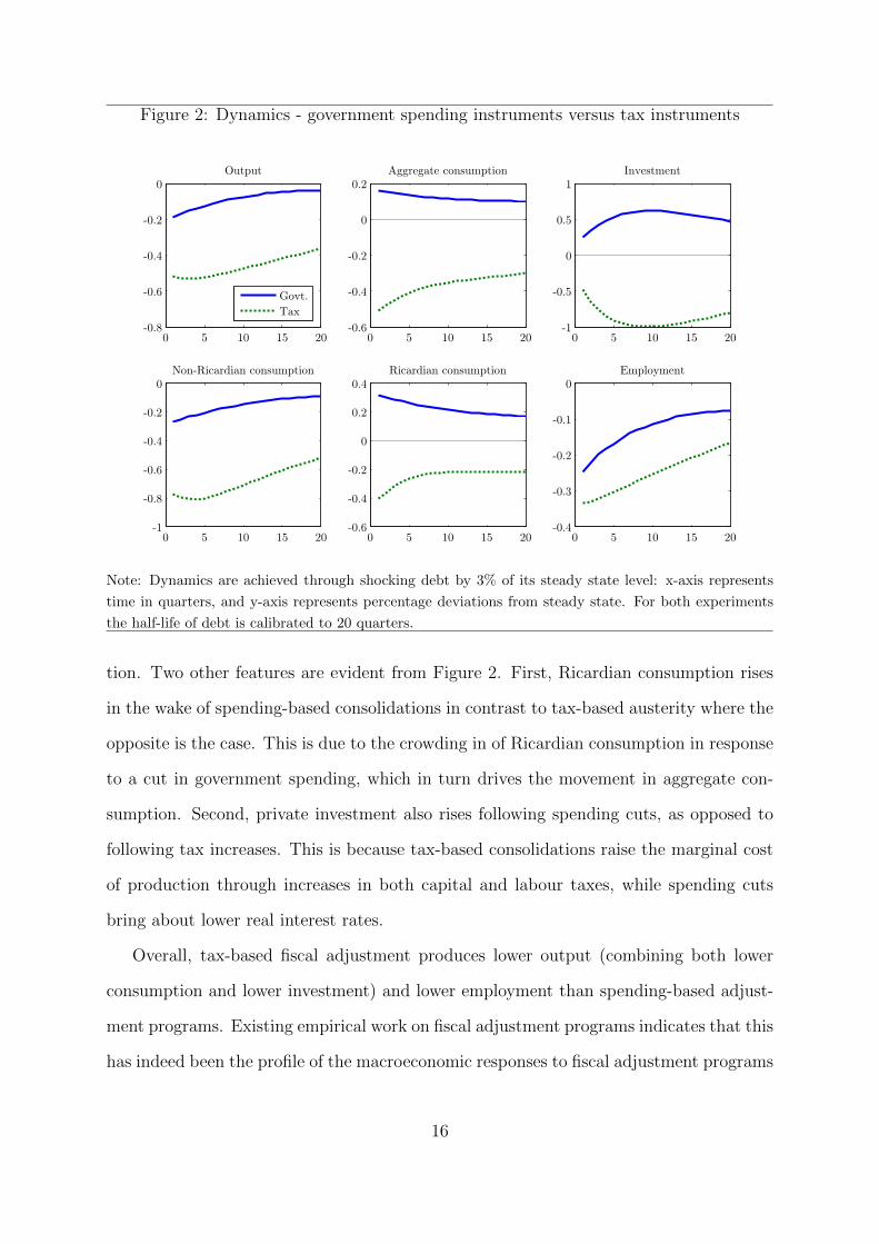
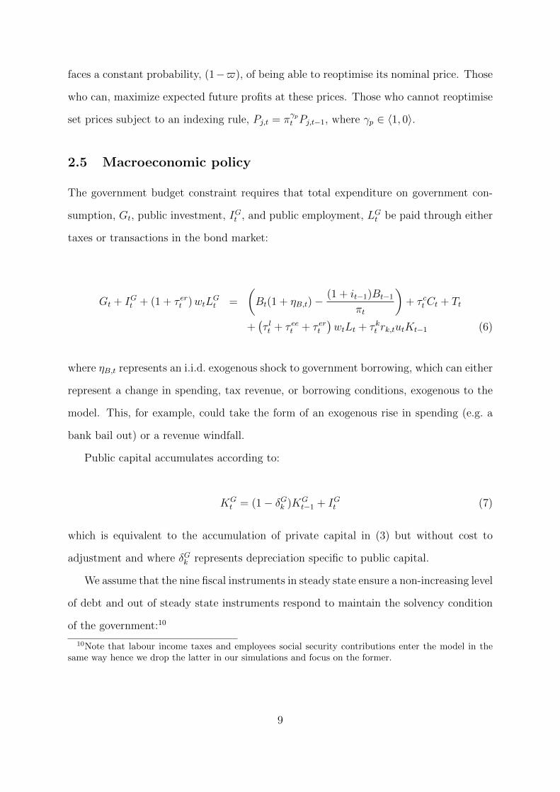
Figure 2: Dynamics - government spending instruments versus tax instruments
0 5 10 15 20-0.8
-0.6
-0.4
-0.2
0Output
Govt.
Tax
0 5 10 15 20-0.6
-0.4
-0.2
0
0.2Aggregate consumption
0 5 10 15 20-1
-0.5
0
0.5
1Investment
0 5 10 15 20-1
-0.8
-0.6
-0.4
-0.2
0Non-Ricardian consumption
0 5 10 15 20-0.6
-0.4
-0.2
0
0.2
0.4Ricardian consumption
0 5 10 15 20-0.4
-0.3
-0.2
-0.1
0Employment
Note: Dynamics are achieved through shocking debt by 3% of its steady state level: x-axis represents
time in quarters, and y-axis represents percentage deviations from steady state. For both experiments
the half-life of debt is calibrated to 20 quarters.
tion. Two other features are evident from Figure 2. First, Ricardian consumption rises
in the wake of spending-based consolidations in contrast to tax-based austerity where the
opposite is the case. This is due to the crowding in of Ricardian consumption in response
to a cut in government spending, which in turn drives the movement in aggregate con-
sumption. Second, private investment also rises following spending cuts, as opposed to
following tax increases. This is because tax-based consolidations raise the marginal cost
of production through increases in both capital and labour taxes, while spending cuts
bring about lower real interest rates.
Overall, tax-based fiscal adjustment produces lower output (combining both lower
consumption and lower investment) and lower employment than spending-based adjust-
ment programs. Existing empirical work on fiscal adjustment programs indicates that this
has indeed been the profile of the macroeconomic responses to fiscal adjustment programs
16

in practice (see, for example, Agnello et al.; 2012; IMF; 2012; Woo et al.; 2013).
3.3 Fiscal austerity and welfare
We now turn to the welfare implications of fiscal consolidations. Figure 3 plots the
welfare of the two types of households against the speed of fiscal adjustment for the two
consolidation packages focusing on just tax and just spending instruments, respectively.
Figure 3: Welfare effects
10 20 30 40 50-0.07
-0.06
-0.05
-0.04
-0.03
-0.02
-0.01
0Non-Ricardian tax decomposition
Half-life of debt
Welfare
10 20 30 40 50-0.07
-0.06
-0.05
-0.04
-0.03
-0.02
-0.01
0
Half-life of debt
Welfare
Ricardian tax decomposition
Consumption
Social security
Labour
Capital
10 20 30 40 50-0.02
-0.01
0
0.01
0.02
0.03
0.04
Half-life of debt
Welfare
Non-Ricardian government spending decomposition
Labour
Consumption
Investment
Transfers
10 20 30 40 50-0.02
-0.01
0
0.01
0.02
0.03
0.04Ricardian government spending decomposition
Half-life of debt
Welfare
Note: Welfare results are expressed as the equivalent of one-period of steady state consumption that
would leave the agent indifferent between living through the shock or forgoing the one period loss.
The bottom line represents the aggregate impact where shaded areas represent the decomposition of
this aggregate into component fiscal instruments. The top row represents welfare from just using tax
instruments and the bottom row just from spending instruments; the left column depicts results for
non-Ricardian households and the right column for Ricardian households.
In Figure 3, the bottom line represents the aggregate impact where shaded areas
represent the composition of this aggregate in individual fiscal instruments that are com-
17

ponents of the fiscal package in each case. As is seen from the first column in Figure
3, austerity reduces non-Ricardian welfare in all cases and the scale of this reduction is
greater the quicker the speed of consolidation. This is due to the fact that non-Ricardian
agents are exposed to austerity through their dependence on the overall health of the
economy through wages and employment, both of which decline in response to austerity.
Moreover, higher labour and consumption taxes and lower transfers (under the tax-based
fiscal adjustments) decrease the disposable income and subsequently the consumption of
the credit-constrained agents.
As is also seen from the bottom right pane of Figure 3, in contrast, spending-based
consolidations result in Ricardian consumers being better off, irrespective of the speed
of adjustment, due to both higher levels of consumption and lower levels of employ-
ment. Consumption is improved following the reductions in interest rates and govern-
ment spending. Households in the model are assumed not to gain utility from government
consumption and public employment and reductions of these, from the perspective of Ri-
cardian agents, leads to welfare improvements as they can crowd in private consumption
and investment. Both consumers are worse off under tax-based consolidations, though
Ricardian welfare dominates that of non-Ricardians unless debt is repaid over long time
horizons. Ricardian agents do not directly respond to movements in transfers and are
therefore less affected by cuts in these than their non-Ricardian neighbours. Overall, the
welfare consequences are unevenly shared by the two types of agents; austerity tends to
harm non-Ricardian households more than the Ricardian households.
An interesting question related to the welfare implications of spending and tax-based
austerity is whether the welfare outcomes vary significantly between adjustments based
on individual instruments. Figure 3 also presents a decomposition of total welfare impli-
cations of austerity, highlighting the contribution made by each fiscal instrument. The
worst case scenario for both households is fiscal adjustment by increases in capital taxes,
resulting in the lowest welfare for each household as it both reduces incomes in the short
run, and impacts on the productive capacity of the economy over the medium term.
18
However, it must also be noted that rises in capital taxes exert a bigger impact on Ricar-
dian households who directly pay this tax. For similar reasons, increases in labour taxes
have large negative normative consequences for non-Ricardian households for whom a
rise directly reduces disposable income. In contrast, austerity through cuts in govern-
ment consumption and government employment produces the two best welfare outcomes.
Figure 3 once again confirms that austerity always harms the constrained households
while the unconstrained are either better off (under spending-based adjustment) or less
worse off than the constrained household (under the tax-based adjustment).
3.4 Fiscal austerity and income distribution
An important aspect of distributional outcomes arising from fiscal policy changes is re-
lated to their implications for income distribution. This is important for two reasons.
First, as is widely recognized, income distribution plays a key role in political and eco-
nomic stability and thus has a wider significance (see, for example, Alesina and Perotti;
1996). Second, income distribution outcomes are more easily measurable than welfare
ones, which enables us to put our results in perspective in light of the existing empirical
findings on the income distribution implications of fiscal adjustment programs.
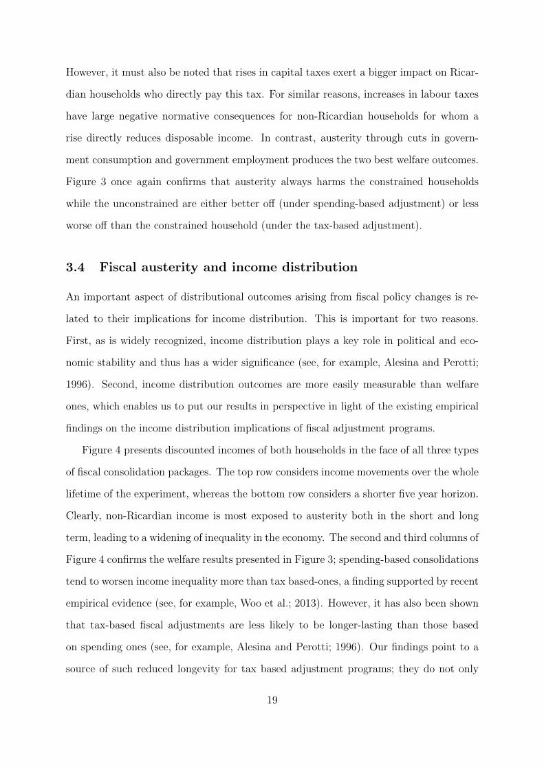
Figure 4 presents discounted incomes of both households in the face of all three types
of fiscal consolidation packages. The top row considers income movements over the whole
lifetime of the experiment, whereas the bottom row considers a shorter five year horizon.
Clearly, non-Ricardian income is most exposed to austerity both in the short and long
term, leading to a widening of inequality in the economy. The second and third columns of
Figure 4 confirms the welfare results presented in Figure 3; spending-based consolidations
tend to worsen income inequality more than tax based-ones, a finding supported by recent
empirical evidence (see, for example, Woo et al.; 2013). However, it has also been shown
that tax-based fiscal adjustments are less likely to be longer-lasting than those based
on spending ones (see, for example, Alesina and Perotti; 1996). Our findings point to a
source of such reduced longevity for tax based adjustment programs; they do not only
19

reduce the welfare of both types of households, they also bring about greater aggregate
fluctuations.
Figure 4: Income effects
0 10 20 30 40 50-0.13
-0.12
-0.11
-0.1
-0.09
-0.08
All instruments: lifetime
Half-life of debt
Discounted income
Non-Ricardian
Ricardian
0 10 20 30 40 50
-0.14
-0.12
-0.1
-0.08
-0.06
Government spending: lifetime
Half-life of debt
Discounted income
0 10 20 30 40 50-0.28
-0.26
-0.24
-0.22
-0.2
-0.18Taxation: lifetime
Half-life of debt
Discounted income
0 10 20 30 40 50-0.1
-0.08
-0.06
-0.04
-0.02All instruments: five years
Half-life of debt
Discounted income
0 10 20 30 40 50-0.08
-0.06
-0.04
-0.02
0Government spending: five year
Half-life of debt
Discounted income
0 10 20 30 40 50
-0.15
-0.1
-0.05
Taxation: five year
Half-life of debt
Discounted income
Note: Discounted income effects under consolidation packages using ‘all instruments’, just ‘Government
spending’ instruments’ and ‘Taxation’ instruments, calculated over the whole lifetime of the experiment
(the top row), and over the first five years of the experiment (the bottom row): future periods are
discounted by relative discount factors.
4 Further extensions
4.1 International consolidation packages
The above results consider the aggregate and distributional impact of fiscal consolida-
tions in a range of benchmark calibrations. In order to obtain a direct perspective on the
austerity measures implemented in recent times, we simulate our model using actual com-
position of fiscal packages based on international data (IMF; 2013, 2014), as summarised
in Table 2.15
15Specifically, we obtain information on the size of fiscal adjustments between 2009 and 2013 fromboth revenue and expenditure measures from IMF Fiscal Monitor (2013: Figure 2) and combine this
20

Table 2: International consolidation data
Debt to GDP Proportions2007 2013 Consolidation Revenue Expenditure
GRC 95.6 173.8 17.8 26% 74%IRL 24.9 122.8 7.6 9% 91%PRT 63.6 128.8 7.4 48% 52%ESP 36.1 93.9 6.9 38% 62%GBR 44.1 90.1 6.2 40% 60%NLD 45.5 74.9 4.6 49% 51%USA 62.1 104.5 4.3 61% 39%FRA 35.2 93.9 3.0 124% -24%BEL 82.8 99.7 2.2 135% -35%AUT 59.5 74.2 1.0 65% 35%DEU 65.0 78.1 0.9 -81% 181%
Note: ‘Consolidation’ represents the sum of both revenue and expenditure based fiscal adjustments,
expressed as the proportion of potential GDP on cyclically adjusted data (obtained from IMF fiscal
monitor); and ‘Revenue’ and ‘Expenditure’ represent the individual proportions of this overall consoli-
dation figure.
Comparing the debt to GDP ratios in 2007 to those in 2013 reveals that there were
significant increases in indebtedness in most countries, where doubling of the debt ratio is
observed in nearly half of the sample. The rise in debt ratios, in turn, required substantial
fiscal adjustment, as large as 17.8 per cent of GDP in Greece, 7.6 per cent in Ireland
and 7.4 per cent in Portugal. An interesting aspect of these consolidation packages
has been the wide variation in their composition. Table 2 suggests that countries that
have carried out substantial adjustment packages such as Greece, Ireland, Portugal and
Spain carried out most of this adjustment through expenditure-based measures while
those with smaller consolidation, with the notable exception of Germany, adopted mostly
taxed-based adjustment.
We employ the same empirical composition of consolidation packages currently in
place in each country and impose the same 3 per cent shock to steady-state government
debt as above over a variety of speeds of repayment. Figure 5 groups the countries into
with data on individual spending measures (IMF; 2014, Figure 2.2) and tax measures (IMF; 2014, Table9).
21

high consolidators (Greece, Ireland, Portugal and Spain), medium consolidators (UK,
Netherlands and US), and low consolidators (France, Belgium, Austria and Germany)
and presents predicted welfare movements, and Figure 6 presents the sum of discounted
output (using βR) from the model.
Figure 5: International comparison: welfare movements
0 20 40-0.1
-0.05
0
AUT
Half-life of debt
WelfareMovements
Non-Ricardian
Ricardian
0 20 40-0.12
-0.1
-0.08
-0.06
BEL
Half-life of debt
WelfareMovements
0 20 40-0.12
-0.1
-0.08
-0.06
FRA
Half-life of debt
WelfareMovements
0 20 40
-0.05
0
0.05
0.1
0.15
GER
Half-life of debt
WelfareMovements
0 20 40
-0.05
0
0.05
GRE
Half-life of debt
WelfareMovements
0 20 40-0.05
0
0.05
0.1
IRE
Half-life of debt
WelfareMovements
0 20 40
-0.05
0
0.05
0.1
NLD
Half-life of debt
WelfareMovements
0 20 40
-0.05
0
0.05
POR
Half-life of debt
WelfareMovements
0 20 40
-0.05
0
0.05
ESP
Half-life of debt
WelfareMovements
0 20 40
-0.05
0
0.05
0.1
UK
Half-life of debt
WelfareMovements
0 20 40
-0.05
0
0.05
US
Half-life of debt
WelfareMovements
Note: Results are obtained by utilizing IMF Fiscal Monitor data on the composition of current fiscal
adjustment packages and assuming a similar composition for future consolidation, and through the same
shock of 3% of steady state debt to aid comparisons. The calibration is as that of Table 1 but where the
fiscal parameters are calibrated differently for the EU countries (where we use Coenen et al.; 2013), the
UK (where we use Bhattarai and Trzeciakiewicz; 2012) and the US (where we use Leeper et al.; 2010).
Figures 5 and 6 enables us to make a number of observations. First, the composition
of consolidation is of far more importance to its positive results, compared to with the
speed of consolidation. In line with our earlier results, those policies which target gov-
ernment expenditure have the lowest impact on output, and as in the case of Germany,
spending cuts to finance some tax cuts can have a beneficial impact to output. Similarly,
Figure 5 reveals that the composition of consolidation is also of much more importance
to its distributive outcomes than its speed; specifically, consolidations which focus on tax
22

Figure 6: International comparison: discounted output
0 5 10 15 20 25 30 35 40 45 50
-0.14
-0.12
-0.1
-0.08
-0.06
-0.04
-0.02
0
0.02
0.04
Discounted Output
Half-life of debt
Disc
ount
ed O
utpu
t
AUSBELFRAGERGREIRENLDPORESPUKUS
Note: Results are obtained by utilizing IMF Fiscal Monitor data on the composition of current fiscal
adjustment packages and assuming a similar composition for future consolidation, and through the same
shock of 3% of steady state debt to aid comparisons. The calibration is as that of Table 1 but where the
fiscal parameters are calibrated differently for the EU countries (where we use Coenen et al.; 2013), the
UK (where we use Bhattarai and Trzeciakiewicz; 2012) and the US (where we use Leeper et al.; 2010).
revenues as opposed to spending cuts have the most equitable normative effects, as is seen
above, and is supported by cross-country simulated evidence. For example, in countries
where fiscal adjustment is carried out mostly through expenditure related measures, as
was the case in high consolidation countries (the top row), the outcome is the substantial
gap in the welfare of the constrained and unconstrained households. This gap is clearly
smaller in low consolidation countries such as Austria, Belgium and France who mostly
utilized tax-based instruments. France is the best example of this with the only consoli-
dation package where non-Ricardian welfare can dominate Ricardian welfare (beyond 30
quarters for the half-life of debt).
Interestingly, the greatest gap between the welfare of the constrained and the un-
constrained households is in Germany who have enacted cuts to transfers, government
consumption and government employment to pay for cuts in income taxes and social
23

security contributions and increased public investment. Germany’s composition also has
a positive impact on output, the only one to do so.
Overall, the trade-off between equity and positive efficiency of fiscal adjustment pro-
grams found above is maintained. Whereas spending-based consolidations can lead to
lower overall effects with respect to output, incomes and welfare, tax-based austerity is
associated with more equality of sacrifice whereby all agents lose more, but do so to-
gether. Although non-Ricardian agents tend to lose less in absolute terms with spending
based programmes than in tax-based ones, the relative welfare considerations carry great
significance in practice. This is illustrated by the political consequences of austerity over
recent years, especially in the high consolidation countries, those which rely more on cuts
in spending; all three countries Greece, Spain and Portugal have witnessed greatest anti-
austerity protests observed across Europe following the adoption of fiscal consolidation.
4.2 Austerity at the zero lower bound
A key distinguishing feature of the recent recession, for which it has received much aca-
demic attention, is that monetary policy has been operating at its lower bound where
nominal interest rates reach, or are close to, zero. Under such a scenario fiscal multipliers
are shown to increase as the contractionary impact of higher interest rates associated
with higher levels of output are removed: see, for example, Eggertsson (2011), Christiano
et al. (2011) and Hall (2011). An interesting question is whether the presence of the zero
lower bound (ZLB) has any impact on the welfare consequences of fiscal consolidation.
Figure 7 presents the welfare movements in three fiscal scenarios: where all fiscal
instruments are used; when only the three production taxes (labour, capital and employer
social security) are used; and when all government spending instruments are used, as well
as consumption taxes. As is clear in Figure 7, the ZLB doesn’t alter the welfare outcomes
to a strong degree. However, at the monetary ZLB the composition of consolidation
becomes more important: if austerity is executed through increases in production taxes
then one can have a more fruitful consolidation as these rises have an expansionary
24

Figure 7: Welfare effects at the zero lower bound
0 10 20 30 40 50
-0.06
-0.04
-0.02
0
0.02
ZLB half-life of debt
Welfare m
ovem
ents
All instruments
0 10 20 30 40 50
-0.14
-0.12
-0.1
-0.08
-0.06
-0.04
-0.02
0
ZLB half-life of debt
Welfare m
ovem
ents
Just production taxes
NRZLB
RZLB
NRBench
RBench
0 10 20 30 40 50
-0.04
-0.02
0
0.02
0.04
0.06
0.08
ZLB half-life of debt
Welfare m
ovem
ents
Govt. spending and consumption taxes
Note: Welfare results are expressed as the equivalent of one-period of steady state consumption that
would leave the agent indifferent between living through the shock or forgoing the one period loss.
The three panes represent the three different experiments from using ‘all instrument’ from using only
‘production taxes’ (labour, capital and employer social security contribution) and from using all spending
instruments and consumption taxes. ‘NR’ and ‘R’ in the legend represent results for non-Ricardian and
Ricardian households respectively and ‘Bench’ represents benchmark results from when the monetary
zero lower bound is not binding.
effect due to the inflationary pressures they provide the economy, thus lowering the real
interest rate: this is a result highlighted in Eggertsson (2011). However, spending based
consolidations, or those focussing on consumption taxes, are worse when conducted at
the ZLB.
However, these results do hide a timing disparity, whereby during the period of the
zero lower bound (which is what Europe, the UK and the US has been of late) the impact
is heightened. Therefore, consolidations based on spending cuts and front loaded will be
felt much worse. It is interesting to note that those high consolidating countries such as
Greece, Ireland and Spain performed the significant majority of their austerity through
spending cuts and in a front-loaded fashion. Over the whole period of consolidation,
however, when the initial phase is averaged out, these effects look smaller.
4.3 Sensitivity analysis
We have simulated our model, both for the positive and normative implications, across
a wide range of parameter values of wage and price stickiness, the proportion of credit-
constrained consumers, Taylor rule parameters as well as the horizon of welfare calcula-
25

tions to better reflect the shorter political horizon. We find that varying these parameter
values has a negligible qualitative and quantitative impact on the results (not reported).
5 Conclusions
This paper explored the aggregate and the distributional impact of fiscal austerity by
utilizing a medium scale DSGE model with a rich set of fiscal instruments. We exam-
ine aggregate, welfare and the income distribution outcomes in different types of fiscal
adjustment that vary with its composition and the speed of adjustment.
Our main results are as follows. First, we find that fiscal austerity gives rise to a va-
riety of distributional outcomes, determined predominantly by the composition of fiscal
adjustment. In almost all cases, austerity tends to harm credit constrained households
more than those with full access to capital markets. We find that spending-based fis-
cal adjustment improves Ricardians’ welfare while non-Ricardians lose out. In contrast,
tax-based fiscal consolidations reduce welfare of both types of households but dispropor-
tionately more of non-Ricardians. In addition to making everyone worse off, tax based
consolidations also bring about greater contractions in output and employment. These
two aspects of tax-based consolidations versus spending-based ones may have important
implications for the continuity of these programs. Indeed, existing empirical literature
on fiscal adjustments presents evidence for tax based consolidations to be shorter lived
than spending based ones.
We also examined the implications of the ZLB on the welfare consequences of fis-
cal consolidations. We find that, inspite of their well-known favourable impact on the
effectiveness of fiscal policy, the presence of the ZLB doesn’t alter the welfare ranking
across different set of consumers following fiscal austerity. However, we also show that
the composition of consolidations gains more importance at the ZLB. For example, we
find that fiscal adjustment through capital taxes are less bad in welfare terms at ZLB,
in contrast to adjustment through government spending or consumption taxes where the
26

opposite is true.
Overall, our findings also point to a clear trade off between the efficiency and the
equity aspects of austerity. Policies that lead to greater aggregate fluctuations (tax-
based) are also those that generate smaller inequality both in terms of welfare and income
distribution. Given the severity of the recent downturn in most advanced economies that
have adopted austerity, and the resulting preoccupation with GDP figures, this trade-off
between growth and distributional consequences of fiscal consolidation is likely to pose
serious challenges to policymakers in many countries.
References
Agnello, L., Mallick, S. K. and Sousa, R. M. (2012). Financial reforms and income
inequality, Economics Letters 116(3): 583–587.
Alesina, A. and Perotti, R. (1996). Fiscal adjustments in OECD countries: composition
and macroeconomic effects, NBER Working Papers No. 5730.
Bhattarai, K. and Trzeciakiewicz, D. (2012). Macroeconomic impacts of fiscal policy
shocks in UK: A DSGE analysis, Technical report, mimeo, University of Hull.
Calvo, G. (1983). Staggered prices in a utility-maximizing framework, Journal of Mone-
tary Economics 12(3): 383–398.
Campbell, J. and Mankiw, N. (1989). Consumption, income, and interest rates: Reinter-
preting the time series evidence, NBER Macroeconomics Annual 4: 185–216.
Christiano, L., Eichenbaum, M. and Rebelo, S. (2011). When is the government spending
multiplier large?, Journal of Political Economy 119(1): 78–121.
Christiano, L. J., Eichenbaum, M. and Evans, C. L. (2005). Nominal rigidities and the
dynamic effects of a shock to monetary policy, Journal of Political Economy 113(1): 1–
45.
27

Coenen, G., Straub, R. and Trabandt, M. (2013). Gauging the effects of fiscal stimulus
packages in the Euro area, Journal of Economic Dynamics and Control 37(2): 367–386.
Cogan, J., Cwik, T., Taylor, J. and Wieland, V. (2010). New Keynesian versus old key-
nesian government spending multipliers, Journal of Economic Dynamics and Control
34(3): 281–295.
Drautzburg, T. and Uhlig, H. (2011). Fiscal stimulus and distortionary taxation, NBER
Working Paper No.17111.
Eggertsson, G. (2011). What fiscal policy is effective at zero interest rates?, NBER
Macroeconomics Annual 25(1): 59–112.
Erceg, C. J., Guerrieri, L. and Gust, C. (2005). Expansionary fiscal shocks and the us
trade deficit, International Finance 8(3): 363–397.
Erceg, C. J., Henderson, D. W. and Levin, A. T. (2000). Optimal monetary policy with
staggered wage and price contracts, Journal of Monetary Economics 46(2): 281–313.
Granados, C. M. (2005). Fiscal adjustments and the short-term trade-off between eco-
nomic growth and equality, Hacienda Publica Espanola (172): 61–92.
Hall, R. (2011). The long slump, American Economic Review 101(2): 431–469.
Iacoviello, M. (2005). House prices, borrowing constraints, and monetary policy in the
business cycle, American Economic Review 95(3): 739–764.
IMF (2012). IMF Fiscal Outlook: Balancing Fiscal Policy Risks, Vol. 2012, IMF Pub-
lishing, Washington, D.C.
IMF (2013). Fiscal Monitor October 2013: Taxing times, Vol. 5, International Monetary
Fund, Washington, D.C.
IMF (2014). Fiscal Monitor October 2014: Public expenditure reform, making difficult
choices, Vol. 6, International Monetary Fund, Washington, D.C.
28

Leeper, E. M., Plante, M. and Traum, N. (2010). Dynamics of fiscal financing in the
united states, Journal of Econometrics 156(2): 304–321.
Mankiw, N. (2000). The savers-spenders theory of fiscal policy, American Economic
Review 90(2): 120–125.
McManus, R. (2012). Austerity versus stimulus: A political economy explanation, Uni-
versity of York Discussion Papers in Economics.
OECD (2009). OECD Economic Outlook, Vol. 2009, OECD Publishing, Paris.
OECD (2012). OECD Economic Outlook, Vol. 2012, OECD Publishing, Paris.
Romer, C. and Bernstein, J. (2009). The job impact of the American recovery and
reinvestment plan, Office of the President-Elect.
Schmitt-Grohe, S. and Uribe, M. (2006). Optimal fiscal and monetary policy in a medium-
scale macroeconomic model, 20: 383–462.
Smets, F. and Wouters, R. (2003). An estimated dynamic stochastic general equilibrium
model of the Euro area, Journal of the European Economic Association 1(5): 1123–
1175.
Straub, R. and Tchakarov, I. (2007). Assessing the impact of a change in the composition
of public spending: A DSGE approach, ECB Working Paper.
Wolff, E. N. (1998). Recent trends in the size distribution of household wealth, Journal
of Economic Perspectives 12(3): 131–150.
Woo, J., Bova, E., Kinda, T. and Zhang, Y. (2013). Distributional consequences of
fiscal consolidation and the role of fiscal policy: What do the data say?, International
Monetary Fund Discussion Paper.
29