Embed Size (px)
Citation preview

DISCUSSION PAPER PI-1003 Estimation and Pricing with the Cairns-Blake-Dowd Model of Mortality Edmund Cannon January 2010 ISSN 1367-580X The Pensions Institute Cass Business School City University 106 Bunhill Row London EC1Y 8TZ UNITED KINGDOM http://www.pensions-institute.org/
Estimation and pricing with the Cairns‐Blake‐Dowd model of mortality Edmund Cannon
Abstract
Parametric forecasts of future mortality improvements can be based on models
with a small number of factors which summarise both the improvement in
mortality and changes in the relationship between mortality and age. I extend the
analysis of the two‐factor model of Cairns, Blake and Dowd (2006) to a more
general dynamic process for the factors and also consider the problems arising
from modelling estimated rather than observed factors. The methods are applied
to mortality data for sixteen countries and are used to estimate the value of an
annuity and measures of risk. The consequences for the money’s worth of an
annuity and reserving are also considered.
Keywords
stochastic mortality, mortality projections, annuity, money’s worth
This research was undertaken during a visit to the Department of Economics at University of Verona, whose hospitality and financial support are gratefully acknowledged. I have also benefited from discussions with Ian Tonks. Any remaining errors are my own.

1. Introduction Recent advances in actuarial practice have resulted in a variety of models for
describing and projecting mortality: a convenient survey and exposition is
provided by Pitacco et al (2009).1 One of the important features of the more
recent models is that mortality projections are stochastic rather than
deterministic. This is important for two reasons. First, the value of an annuity or
any similar pension‐type product is a non‐linear function of future mortality and
hence calculations of annuity values should be based upon the entire distribution
rather than just the expected future mortality. Secondly, risk management
requires knowledge of the distribution of the annuity and this can only be
calculated with knowledge of the mortality distribution. This paper describes
several important modelling, estimation and forecast issues within the context of
the model proposed by Cairns, Blake and Dowd (2006) (which I shall refer to as
the “CBD model”). Most of the results have wider applicability.
The CBD model is a “two‐factor” model and is one among a large number of
contenders for projecting mortality. The underlying idea is that there is a
(downward) trend in mortality, which is presumably either a stochastic trend or a
deterministic trend with some variation about the trend. If improvements in
mortality were perfectly correlated at all ages then it would be possible to project
mortality using a “one‐factor” model such as the simple Lee‐Carter (1992) model.
However, improvements in mortality do not just consist of downward shifts in the
functional relationship between mortality and age but also changes in the “shape”
of the relationship. If this relationship were sufficiently complicated, or the
changes were sufficiently complicated, then this might need to be modelled non‐
parametrically. This is the P‐spline type approach of Eilers and Marx (1996) or
CMI (2006). However, empirically it is possible to approximate well the
relationship between mortality and age by fairly simple functional forms involving
relatively few parameters (Cairns et al, 2009). In the simplest case only one
1 Of course, this does not mean that practising actuaries actually use these new models. CMI (2009, p.6) reports that 83% of life insurers and 82% of pension funds still used a particular version of the deterministic projections made by the UK’s Institute of Actuaries in 1999 and up‐dated in CMI (2002).

parameter is needed to describe the relationship and hence mortality projection
requires two factors, which jointly provide a description of the relationship
between mortality and age and the trend in mortality over time.
This results in a wide variety of modelling strategies: should the model predict log
mortality or the log‐odds of mortality (e.g., Cairns et al, 2009); should there be
two or more factors (e.g., Plat, 2009, suggests four); should there be additional
cohort effects (Renshaw and Haberman, 2006)? Merely surveying a sub‐set of
these possibilities takes up a substantial number of pages in Pitacco et al (2009).
However, any n‐factor model (with n equal to a small number greater than one,
such as two) will face the question of how the factors evolve over time and it is
this question that I consider here. In the simplest case of two factors, there are
three possibilities: both factors are stochastic trends (the original CBD model);
both factors vary stochastically about deterministic trends (Sweeting, 2009); or the
factors are stochastic trends but share a unit root so that they are cointegrated.
In section 2 of this paper I shall provide an exposition of the model under all three
cases in Section 2. A consequence of this class of model which has not received
much attention in the literature is that there is ambiguous relationship between
the variance of mortality forecasts and the expected value of an annuity: I prove
this in section 3. In section 4 I discuss the application of the two factor model to
mortality data for sixteen countries taken from the Human Mortality Database. In
section 5 I discuss the problems that arise from the fact that the CBD methodology
first estimates the factors and then analyses their dynamic properties: in the light
of this I report tests for distinguishing the models and quantify the importance of
measurement error. The resulting analysis provides estimates of annuity values,
measures of risk and measures of the consequences for the money’s worth of
annuities actually sold. Section 6 discusses my results and concludes.
2. An outline of the two‐factor model The CBD model works with a logistic transform of death probabilities or death
rates. Given constraints on data availability it is often necessary to work in a
discrete‐time model with such variables and accordingly in this paper I work
consistently with one‐year death probabilities, where ,x tq is the probability of
dying within one year for someone aged x in year t and , ,1x t x tp qº - . 2 The
original CBD model uses period rather than cohort life tables and can be written
(1) ( ) { } { }1 2, ,ln 60,..., 95 , 0, ..., 1x t x t t tq p A A x x t T= + Î Î -
where the choice of ages 60 to 95 is driven mainly by considerations of data
availability and partially to reduce problems of heteroskedasticity which occur
when very high ages are included.
Equation (1) says that the log‐odds of death probabilities for different ages in year
t is a linear function of age, where both the intercept 1tA and the slope 2
tA of the
linear function can vary through time. At the risk of stating the obvious, because
this is a model of different ages at the same point in time, it is using data from
cohorts born in different years. 1tA and 2
tA are the two “factors”. In practice it is
impossible to observe either factor, so they must be estimated: CBD do this using
OLS although alternative procedures are available.3 In this section I ignore the
problem of estimation. In a generalisation of the CBD model, the evolution of the
two factors through time is modelled by
(2) 1 1 1 1 1 1
11 12 1 11 122 2 2 2 2 2
21 22 12 221
0~ ,
0t t t t
t t t t
A A v vt
v vA Ap p m d z zp p m d z z
-
-
ææ ö æ ö æ ö æ ö æ ö æ öæ ö æ ö æ ö÷ ÷ ÷ ÷ ÷ ÷÷ ç ÷ ÷ç ç ç ç ç çç ç ç÷ ÷ ÷ ÷ ÷ ÷÷ ÷ ÷çç ç ç ç ç çç ç ç= + + +÷ ÷ ÷ ÷ ÷ ÷÷ ÷ ÷ç ç ç ç ç çç ç ç÷ ÷ ÷ ÷ ÷ ÷÷ ÷ ÷ç ç ç ç ç çç ç ç÷ ÷ ÷÷ ÷ ÷ ÷ ÷ ÷ç ç çç ç ç ç ç çè ø è ø è øè ø è ø è ø è ø è ø è ø èN
ö÷÷÷ç ÷ç ÷÷ç ø
To simplify notation I re‐write equations (1) and (2) respectively as
(3) t t=Q XA
(4) ( ),1 , ~t t t tt-= + + +A A 0 VNp m d z z
where
2 The relationship between one‐year death probabilities, death rates and mortality, are discussed in actuarial texts such as Bowers et al (1997) or Pitacco et al (2009). 3 A simple alternative to control for heteroskedasticity would be GLS; when information on the exposed‐to‐risk is also available a more efficient estimator would explicitly model q with the binomial distribution.

(5)
( ) ( )
60, 99,
60, 99,
11 121 2 1 2
21 22
1 1 ... 1 1ln ... ln , ,
60 61 ... 991 1
, , , , ,
t tt
t t
t t t
q qxq q
A A etc etcp p
m mp p
¢ ¢ ¢æ öæ ö æ ö æ ö æ ö÷ç ÷ ÷ ÷ ÷ç ç ç ç÷÷ ÷ ÷ ÷ç ç ç ç çº º =÷÷ ÷ ÷ ÷ç ç ç ç ç÷÷ ÷ ÷ ÷ç ç ç ç ç÷- - ÷ ÷÷ ÷ ç çç ç ÷ç è ø è øè ø è øè ø
æ ö¢ ¢ ÷ç ÷çº º º ÷ç ÷ç ÷çè ø
Q X x
A m p
I is the identity matrix and 0 a vector of zeros. With appropriate estimators of
the parameters, this model can be used to predict numerically the density function
of the factors using equation (4).
The crux of the matter is how to model equation (4), the interpretation of which
depends crucially upon the rank of the matrix - Ip . CBD assume
(6) ( )1 , 0t t t-= + + - =A A Irankm z p
i.e. the two factors are independent random walks with drift (stochastic trends),4
whose only possible relationship is contemporaneous correlation in the shock
terms through non‐zero off‐diagonal components of V .5 Two obvious alternative
parameterisations are
(7) ( ) ( )
( ) ( )1
1 2
, 1
, 1
t t t
g g b
-D = - + + - =
¢= - º º º
A I A I
0 I
rankp m z p
d p gb g b
(8) ( ), 2t t tt rank= + + + - =A A Ip m d z p
The second of these assumes that both factors are deterministic trends (rather
than stochastic trends), whereas the first assumes that there is one stochastic
trend and the two factors are cointegrated.
A special case of (8) is that = 0p , which is considered by Sweeting (2009) in the
context of a model where the parameters m and d are subject to infrequent and
stochastic shifts.
4 When the system in equation (4) has ( ) 0,1- =Irank p it is assumed that =d 0 and the
stochastic trend is modelled by the parameter m; when ( ) 2- =Irank p the deterministic
trend is modelled by the parameter d . 5 In my analyses I find that the correlation between 1ˆ
tz and 2ˆtz from model (5) is almost
unity (as do CBD), which may suggest that the model be under‐parameterised.

3. Pricing an annuity In this section I discuss the use of the two‐factor model for valuing a financial
product, specifically an annuity (although it could also be used to value products
such as a mortality bond as in the original CBD article).
Consider a simple life annuity paying an annual income of one unit per period in
arrears without proportion. The general formula for the expected value of an
annuity sold at time T is
(9) 1
, ,01
i
x T T i x j T jji
a R p¥ -
+ + +==
= å Õ %
where R is the discount factor for term‐to‐maturity i. In actuarial textbooks this is
often assumed to be the same for all terms but in economists’ analysis of the
money’s worth it is usually taken from estimates of the yield curve. The future
probabilities are unknown and have to be projected, denoted by ,x j T jp + +% . To
simplify notation, and without loss of generality, I assume that the maximum
number of periods that the annuitant will live is two so equation (9) can be
written
(10) , 1 , 1 , 1, 1x T x t x t x ta R p R p p + += +
Note that when the annuity is sold the most recent data available will be for
period 1T - (in practice the most recent data available will be older than this).
3.1 Deterministic projection
The simplest projection methodology would be to ignore all of the uncertainty.
Then
(11)
{}
{} {} ( ){} ( ) {}{ }( )
{} ( ) {}{ }( ){} {} {} {}
11
1 11
11 1,
11 1
1, 1 1
1 1 1 1, 1 , 1 , 1, 1
ˆˆˆ
ˆˆˆ 1
1 exp 1
1 exp 1 1
T T
T T
x T T
x T T
x T x T x T x T
T
T
p x
p x
a R p R p p
-
+
-
-
+ + +
+ +
= + +
= + + +
= +
= + +
= +
A A
A A
A
A
p m d
p m d
%
% %
%%
%%
% % %

where the superscript {1} denotes the method of calculating the annuity.6 This
method of calculation is similar to the projections methods used in the UK in the
construction of the “80”, “92” or “00” tables, where a statistical estimation method
was used to estimate a relationship between mortality and age and then projected
forward deterministically using a trend.7
3.2 Stochastic projection taking parameters as certain
The uncertain nature of the factors can be modelled using
(12) {}
{} { } ( )
21
2 21 1
ˆˆˆ
ˆˆˆ 1
T T T
T T T
T
T
-
+ +
= + + +
= + + + +
A A
A A
p m d z
p m d z
% %
% % %
where the density function of the factors can be simulated by generating pseudo‐
random values for the shock terms from the estimated distribution
( )1ˆ, ~ 0,T T + VNz z% % . In the simulations below I generate 100,000 simulations allowing
me to calculate 100,000 values of the annuity using
(13)
{ } ( ) {}{ }( )² {} ( ) {}{ }( )
( ) {}{ }( ){ } {} ² { }
12 2,
12 2, 1, 1
12
1 1
22 1, 1 , 1 , 1, 1
1 exp 1
1 exp 1
1 exp 1 1
x T T
x T x T T T
T T
x T x T x T x T
p x
p p x
x
a R p R p p
e
e
-
-
+ +
-
+ +
+ +
= +
= + +
´ + + +
= +
A
A
A
%%
%
%
%
Note that this method involves generating the survival probabilities to each age
rather than each annual survival probability: the latter would substitute (13) by
(14) { } ( ) {}{ }( )
{ } {} {} { }
12 2
1, 1 1 1
2 2 2 2, 1 , 1 , 1, 1
1 exp 1 1Bx T T T
B Bx T x T x T x T
p x
a R p R p p
e-
+ + + +
+ +
= + + +
= +
A%%
% % %
6 Note that in models (6) and (7) there is no d term. 7 The trend was based on data supplemented by judgements about ceilings or floors on mortality or mortality improvements. One of the most recent publications by the UK actuarial profession advocates this approach (CMI, 2009).

and hence ignore the correlation between the survival probabilities in different
periods.8
3.3 Stochastic projection taking parameters as uncertain
The final possibility is to acknowledge that the parameter values are themselves
estimates and hence uncertain. Then
(15) { }
{ } { } ( )
31
3 31 11
T T T
T T T
T
T
-
+ +
= + + +
= + + + +
A A
A A
p m d z
p m d z
%% %%%
%% % %%%
In each of my 100,000 simulations I draw a set of parameters from their assumed
distribution and then add the pseudo‐random shock terms. Generation of the
parameter values is slightly different in each model (6), (7) and (8) and is detailed
in the appendix. Finally
(16)
{ } ( ) { }{ }( )² { } ( ) { }{ }( )
( ) { }{ }( ){ } {} ² { }
13 3,
13 3, 1, 1
13
1 1
33 1, 1 , 1 , 1, 1
1 exp 1
1 exp 1
1 exp 1 1
x T T T
x T x T T T
T T
x T x T x T x T
p x
p p x
x
a R p R p p
e
e
e
-
-
+ +
-
+ +
+ +
= + +
= + +
´ + + +
= +
A
A
A
%%
%
%
%
3.4 Relationship between the different valuations
Perhaps surprisingly there is no reason to believe that incorporating risk has an
unambiguous effect on the value of the annuity. The reason for this is that the
annuity formulae in equations (13), (14) and (16) may be concave functions of the
risk in mortality improvement: the concavity or otherwise of the function depends
upon the actual survival probabilities and interest rates. By a standard application
of Jensen’s inequality, a value function which is a concave function of a stochastic
variable will have a negative relationship to the variance of the variable. To see
this, rewrite equation (10) as
(17) 1 2
2, 1
11 1x T F F
Ra R
e e
æ ö÷ç ÷ç= + ÷ç ÷÷ç+ +è ø
8 From the equation on page 694 of CBD it appears that they used the method in equation (14) rather than that in equation (13).

where the stochastic component is 1 21 1i T i T iF A A x- + - += + . The relevant derivatives
are
(18)
( )
( )( )( )
( )( )
( )( )
1
21
2
1 2
1 1
21
2
1 2
1
212
1
22
2
121 22
1 12 31 21
122 2 2
12 32 22
22
1 2
011
01 1
1 0011
1 001 1
F
FF
F
F F
F F
FF
F
F F
F F
Ra e RF ee
R eaF e e
e e qRa RqF ee
R e qaqF e e
R e eaF F
æ ö¶ - ÷ç ÷ç= + <÷ç ÷÷ç¶ +è ø+
-¶ = <¶ + +
ì- æ ö ï < Û <¶ ÷ ïç ÷ç= + í÷ç ÷ ï > Û >÷ç¶ +è ø ï+ î
ì- ï < Û <¶ ï= íï > Û >¶ ï+ + î
¶ =¶ ¶ ( ) ( )
2
1 22 2
01 1F Fe e
>+ +
Thus both of the diagonal elements of the Hessian matrix will be negative if the
probability of dying in the first period is sufficiently low, namely less than one‐
half. From 1970 onwards in the UK such high death probabilities were only found
among men aged 96 or more and this is also true for most other developed
countries. For the function to be concave function, the Hessian would need to be
negative semi‐definite. From the derivatives in (27), the determinant of the
Hessian is
(19) ( )( )
( )( ){ }
1 1 2
1 2 1 2
2 2 221 1 2
2 2 2 11 2 2
2 22
det 1 1
1 1 0
F F F
F F F F
a F a F FR e e e
a F F a F
R e e e +
æ ö¶ ¶ ¶ ¶ ¶ ÷ç ÷ç µ - -÷ç ÷ç¶ ¶ ¶ ¶ ¶ ÷çè ø
+ - - - £
so it is quite possible that the function will be concave, confirming that the effect
of the variance on the value of the annuity is ambiguous.
4. Data and preliminary discussion of the model In the rest of the paper I apply the CBD model and its extensions to male
population mortality data taken from the Human Mortality Database for sixteen

countries for which good data are available and which are representative of most
developed countries. In this section I briefly introduce the data.
The England & Wales log‐odds data is plotted for the whole period in Figure 1,
which confirms that the log‐odds is an approximately planar surface in age‐year
space. There is sufficient detail in the graph to see an oblique kink running
through the data for the cohort aged 60 in 1985 (born 1925), suggesting that there
may be a significant cohort effect as noted in Willets (2004). An obvious
extension to this paper would be to replicate the analysis using cohort data.9
Figure 1 about here
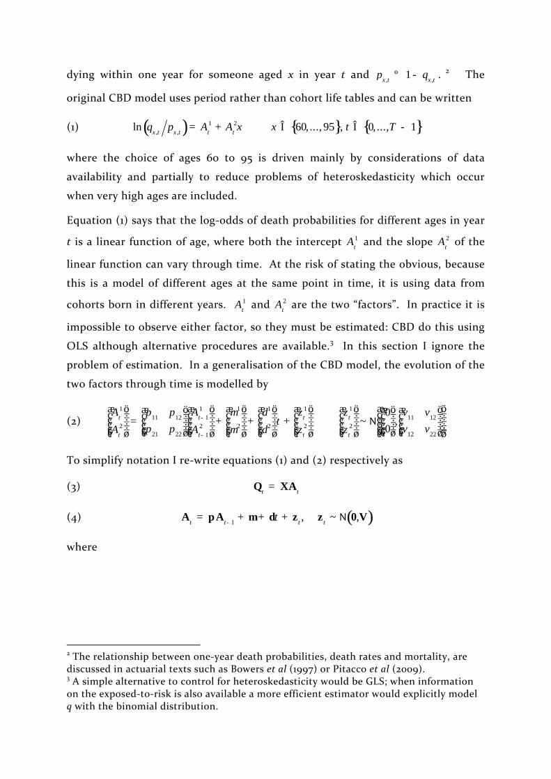
Figures 2 and 3 illustrate my calculated values of the two factors for all sixteen
countries: the first figure shows how the factors evolve over time and second is a
scatter plot joining temporally consecutive points. Visual inspection shows that
there is a large structural break in the trend for most countries in the middle of
the post‐war period. For nearly all countries the time‐series plot for the second
factor is almost a mirror image of that for the first factor. This is confirmed in the
scatter plots where the points lie close to a straight line, although in many
countries the scatter plot appears to be in the shape of a letter “V” lying on its
side.
Certainly over the period 1980 onwards and possibly for the whole period there
appears to be a fairly tight relationship between the two factors. This could be
either because models (7) or (8) fit the data better than model (6), or because
model (6) is correct but the magnitude of the drift terms, m, is large relative to the
variance of the shocks in the random walk process.
Figures 2 and 3 about here
The data for the USA are particularly problematic: while sharing many of the
features present in the data for other countries, there is an additional change in
behaviour of the factors after 2000. Having been in decline from about 1975
onwards the first factor 1tA starts to increase and the opposite happens for the
second factor. At the same time the relationship between these two factors
changes as can be seen from the cross‐plot in Figure 3. Such a change in 9 This would introduce further complications since the factors for the youngest cohorts would have to be estimated from fewer data observations.

behaviour would be difficult to reconcile with any model and it is unsurprising
that the CBD model is unable to fit these data.
5. Analysis of the CBD model and extensions 5.1 Measurement error in the factors
The analysis so far in both this paper and CBD has assumed that the factors are
perfectly observed, but in fact they have to be estimated. Consider replacing
equations (1) and (3) with
(20) ( )2~ ,t t t t w= +Q XA 0 INe e
Using a “hat” to denote the fitted values of the factors,
(21) ( ) ( )1ˆ ~ ,t t t t t t t t t
-¢ ¢º = +A X X X X Q A 0 HNh h
where the vector th can be interpreted as a form of measurement error.10
Substituting (10) into (4) one obtains
(22) 1 1 1ˆ ˆ ˆ
t t t t t t tt t- - -= + + + + - = + + +A A Ap m d z h ph p m d x
leading to the standard result that the OLS estimator is inconsistent, since
(23) OLS 1
1 1ˆ t t
-
- -
æ öé ù é ù ÷¢ç= - ÷ê úç ÷ê ú ë ûë û è øI H R Rplim Ep p
where tR are the residuals obtained from regressing ˆtA on a constant and a
trend.11
There are only two cases in which the OLS estimator will be consistent. If =p 0
there is no problem, but this is implausible and rejected by the data. If the
assumption of the original CBD model, namely = Ip , be true it is unnecessary to
10 Visual examination of the estimated errors suggests mild heteroskedasticity, but I ignore that here to save space. Measurement errors are usually assumed to be serially uncorrelated. 11 Since tx is orthogonal to the constant and the trend they can be “partialled out”. Notice
that 1 1t t- -é ù¢ê úë ûR RE only has a limiting distribution if the data generating process is that of
equation (8), but ( ) 1
1 1t t
-
- -é ù¢ê úë ûR RE has a limiting distribution regardless of the DGP.

estimate p and it is possible to obtain unbiased estimates of m.12 Continuing with
the general case it follows that
(24) ( )( )1 1t t t t t t t t- -
é ù¢é ù ê ú¢ ¢= + - + - = + +ê úë û ê úë ûV H HE Ex x z h ph z h ph p p
showing that the true residuals from the second‐stage regression are a
combination of the stochastic evolution of the factors and the measurement error.
In the special case of the CBD model (equation 6) the OLS estimates are unbiased
and the right hand side of equation (24) simplifies to 2+V H , so a possible
estimator for the relevant matrix would be
(25) 1
1
0
ˆ ˆˆ ˆ2T
t tt
T-
-
=
¢= -åV Hx x
where an estimator for H could be obtained from the first‐stage regressions
(26) ( ) ( ) ( ) ( )12 2, ,
ˆˆ ˆ ˆˆ , ˆ 34t x t x t Tw w- ¢é ù ¢= =ê úë ûH A X Xvar vec vec= e e
Unfortunately there is no guarantee that the expression in equation (25) will be
positive definite and using the data discussed above (from 1980 onwards) it is so
for only the Netherlands and Norway. In fact for some countries even the diagonal
elements of equation (25) – that is the variances – are negative. This problem
could arise either through sampling error or because the simple CBD model is
incorrect: regardless of the cause of the problem, the consequence is that it is
impossible to implement a logically consistent version of the CBD model for most
of the countries in my sample using OLS alone.13
For models (7) or (8) projecting mortality is more complicated. Using equation
(23) a possible estimator for p would be
(27)
11
11 1
1
ˆ ˆ ˆ ˆˆ ˆT
t tt
T
--
-- -
=
æ öæ ö ÷ç ÷ ÷çç ¢ ÷ ÷= - çç ÷ ÷çç ÷ ÷çè øç ÷çè øåI H R Rp p
12 The estimates are unbiased (rather than just consistent) in this case because the only regressor is a constant, which is obviously fixed in repeated samples. 13 The possibility of this problem arises due to estimating the parameters in a two‐stage procedure: first estimating the A parameters and only secondly estimating their dynamic properties. This might be avoided if both were estimated simultaneously (perhaps through Maximum Likelihood), but such an extension is beyond the scope of the current paper.

where for model (8) p̂ would be the OLS estimate from the VAR and for model (7)
p̂ could be the estimate with ( ) 1- =Irank p imposed. The variance might then be
estimated using
(28) 1
1
0
ˆ ˆˆ ˆ ˆ ˆ ˆˆ ˆ ˆˆ ˆT
t tt
T-
-
=
¢ ¢= - -åV H Hx x p p
where the estimated residuals are those obtained using ˆ̂p rather than p̂ . This
formula is only positive definite for Denmark and Norway. Again the problem
arises partly from sampling error:, at best the expressions in equations (27) and
(28) would be consistent and the sample size available is relatively small.
5.2 Distinguishing the models
My analysis so far has considered three versions of the CBD model, based on the
three possibilities for the rank of the matrix - Ip . If these models were to result
in very similar valuations of pension or life products then it would not matter
which were used: but for some data sets the models give very different answers, so
some guidance is needed on which model to use.
An obvious first step is to test the estimated factors for a unit root individually.
Table 1 reports Dickey‐Fuller statistics for these series for each country,
accompanied by conventional p‐values for the test under the null hypothesis of a
unit root. For six countries (Australia, Belgium, France, Germany, Spain and
Sweden) the null of unit roots is comprehensively rejected for both factors and it
is marginal for a further two (Poland and Switzerland). This result appears similar
to that of Sweeting (2009) although he obtained different results for England &
Wales.
However, all of this analysis assumes that there is no measurement error in the
factors. I re‐calculate the p‐values under the null hypothesis assuming that there
is measurement error, where the variances of the shocks driving the unit root and
the measurement error are estimated using equations (25) and (26): this procedure
is only possible where the resulting estimated variance of the shocks is positive.
Of the countries for which the exercise is possible, only Australia and Belgium
appear unambiguously not to have unit roots, with mixed evidence for the
Netherlands and Sweden. Failure to reject the null of a unit root does not appear
to be due to unduly low power: the final column calculates the power of the test

under the alternative hypothesis that the auto‐regressive parameter is 0.9 and
these figures seem acceptable given the small sample sizes.
If there be a unit root it is now necessary to distinguish model (6) from model (7):
are the two factors cointegrated? Johansen (1988, 1995) provides a ML procedure
to distinguish the models in equations (6), (7) and (8) using the estimated
eigenvalues of - Ip to construct the trace statistic:14 this test is just the multi‐
variate extension of the Dickey‐Fuller test. The null hypothesis is that equation
(6) is correct: the alternative hypothesis is that either one or both eigenvalues are
non‐zero.15 The univariate analysis in Table 1 suggests that measurement error has
a big effect on the correct size of tests and this will presumably be true for
multivariate tests also.
The asymptotic 5 per cent critical value when there is no measurement error is
25.32 and the trace statistics for the Netherlands and Norway respectively are
29.88 and 14.86, which would suggest rejecting the null for the Netherlands. This
is prima facie consistent with the result that the Dutch factor 2ˆtA does not have a
unit root when tested in isolation. However, the critical value is too small when
there is measurement error, since this biases the test towards rejecting the null.
Using the estimated parameter values for these two countries a Monte Carlo
experiment suggests that the correct critical values should be 39.18 and 32.10
respectively, so it is impossible to reject the null hypothesis of the model in
equation (6).
As noted in the previous section, the Netherlands and Norway are the only two
countries for which equation (25) can be used to obtain a positive definite V̂ , and
hence the only two countries for which I can construct confidence intervals under
the assumption of measurement error. Thus for Norway and (to a lesser extent)
the Netherlands, the mortality data for these countries appears consistent with the
original CBD model. For the other countries the problem remains that the
procedures used here are insufficient to obtain a satisfactory estimator of the
14 Note that, due to non‐linearity, the ML estimates of the eigenvalues are not the same as the eigenvalues of the ML estimator ˆ - Ip . 15 The Johansen VAR regression includes a trend restricted to lie in the cointegrating space since, under one of the alternative hypotheses (model 8), there must be such a trend for the model to fit the data.

variance using either V̂ or ˆ̂V so it is impossible either to distinguish the models
or use them for valuing an annuity.
5.3 Annuity valuation using different versions of the two‐factor model
Given the problems in operationalising the model when there is measurement
error in the factors, I start by ignoring the problem (ie imposing the assumption
that H = 0 ). While this is not ideal it does allow me to make some comparisons
of the different models under discussion. So I use the models in equations (6), (7)
and (8) with post‐1980 data for all sixteen countries to generate the annuity values {}2a and { }3a . The annuities are valued assuming a constant interest rate of 3 per
cent. As has been discussed above, there are particular problems with the data
from the USA, but I continue to include that country for purposes of comparison.
The simulated expected values, together with the upper and lower deciles and the
90:10 spread, are reported in Table 2 and the density plots are illustrated in
Figures 4, 5 and 6. Perhaps surprisingly, the median value is usually close to the
mean value and the distributions are approximately symmetric although there is
some strange behaviour in the tails (of course these are the parts of the
distribution which are modelled least well).
Figures 4, 5 and 6 about here
Table 21 about here
The expected value of the annuity tends to be highest using the model with
( ) 2- =Irank p and lowest using the model with ( ) 1- =Irank p , but there are many
exceptions to this generalisation. To emphasise the very different annuity prices
of the three models I look at the “spread”, ie the difference between the largest
and smallest expected values from the three models divided by the average
expected value. So for England and Wales the annuity is valued (with parameter
uncertainty) as either 15.68, 15.35 or 15.55 depending on which model is used: a
difference of 0.34 between the highest and lowest price, equal to 2.2 per cent of
the annuity value, clearly a large discrepancy. Where the “spread” is greater than
two per cent it is shaded in the table, which occurs for seven countries other than
the USA. The latter is notable in that the model with ( ) 2- =Irank p fits so badly
as to be nonsense, unsurprisingly given the behaviour of the A factors for that

country shown in Figures 2 and 3: interestingly despite the strange behaviour of
the estimated factors model (6) still provides “plausible” densities, suggesting that
analysis of this model in isolation may prompt an inappropriate reliance on the
results of the model.
For all countries, the result of modelling parameter uncertainty is fairly small:
what changes when parameter uncertainty is introduced is the 90:10 spread. In
section 3 I established that the effect of greater variance in the mortality has an
ambiguous effect on the annuity price. From the table it can be seen that greater
variance tends to increase the price slightly under model (6) but reduce the price
slightly under model (8): ie the effects are opposite for the two models which I
tended to find difficult to choose from the unit root tests.
For either prudential or regulatory reasons a life insurer might sell an annuity not
at the actuarially fair price but at a higher price which would limit the probability
of a policy making a loss: for example, the price might be set to ensure that the
policy be expected to make a loss only 10 per cent of the time. This is one of the
possible reasons why the “money’s worth” which is observed for annuity price
quotes is less than one (Cannon and Tonks, 2008). Note that the money’s worth is
conventionally calculated assuming the expected value of the annuity, whereas the
prudential pricing I have described would result in prices based on the upper
decile. So to calculate the resulting money’s worth, I simply calculate the ratio of
the expected value to the upper decile, using the numbers in Table 2 with
parameter uncertainty. This assumes that there no other transactions costs or
reasons for unfair pricing such as adverse selection. The results are reported in
Table 3. Excluding the special case of the USA, it can be seen that the money’s
worth would be in the range 93 to 97 per cent if life insurers were using model (6).
This is an upper bound to the money’s worth since there may be additional
mortality variance (which I have not modelled) arising from the possibility of
future structural breaks such as that which appeared to occur in the late 1970s for
many countries. Cannon and Tonks (2008, chapter 6) survey money’s worths for
different countries and time periods and find that the money’s worth is typically in
the range 80 to 100 per cent and a rough average would be 90 per cent.
Comparing the figures for model (6) in Table 3 to a money’s worth of 90 per cent
would therefore suggest that reserving against unexpectedly high mortality is

playing a relatively large rôle in low money’s worths. Consequently problems such
as transactions costs, adverse selection or other market failures may be less
important than assumed by economists until now.
Table 3 about here
I now turn to the issue of measurement error and calculate the annuity values for
the Netherlands and Norway (ie the two countries for which I can estimate the
matrix V using equation 25). Results for these countries under model (6) are
reported in Table 4, where I calculate annuity values on the assumption that
parameters of the underlying processes are uncertain. The differences between
the calculations that assume measurement error and those that explicitly model it
are surprisingly small. This provides some evidence that measurement error in the
factors is quantitatively unimportant.
Table 4 about here
6. Conclusion In this paper I have extended the Cairns, Blake and Dowd (2006) two‐factor model
in two important ways: first, to generalise the dynamic processes underlying the
modelling of the factors; and secondly, to account for the measurement error
arising from using estimated rather than observed factors. The two‐step
procedure used by CBD means that there is no guarantee that estimators of the
relevant covariance matrices will be logically admissable (i.e., positive definite)
and thus it is impossible to separate the errors in the dynamic process from the
measurement error. This is most likely due to be sampling error arising from the
short time‐series data available. Where it is possible to estimate the covariances,
the effect on annuity valuation appears to be minimal, so this problem does not
appear to be a major one.
However, the effect of measurement error does have important implications for
tests to distinguish the models. Contrary to the results of Sweeting (2009) I find
adequate evidence that the factors do follow unit root processes for most countries
and my results differ due to the measurement error issue. However, I agree with
Sweeting’s analysis that there appears to be a structural break in about 1980 and
incorporating this into a unit root framework is clearly a job for future research.

The choice between models can have significant differences in the estimated value
of an annuity with differences of up to 2 per cent arising purely from model
uncertainty (and this is model uncertainty within the class of log‐odds‐mortality
two‐factor models).
Increased uncertainty within a model does not necessarily mean that an annuity
will be more costly (in the sense that its expected value is higher), since the effect
of the variance is ambiguous. My simulations in Table 2 demonstrate that this is a
practical possibility since greater uncertainty, arising from explicit modelling of
parameter uncertainty, can increase or decrease expected annuity values. This has
important implications for pricing of annuities by life insurers and monitoring of
annuity prices by government regulators.16
International evidence suggests that the money’s worth of annuities (the price at
which they are actually sold compared to the expected actuarial value) is less than
one. Although there are other reasons for low money’s worths, this could arise
from purely prudential motives of the life insurer or be required by a regulator
who was concerned about the solvency of life insurers if realised mortality was less
than expected when the annuities were sold. Cannon and Tonks (2009) quote a
letter from the UK regulator (the Financial Services Authority) explicitly asking
life insurers to build in adequate safeguards against insolvency. Although widely
recognised as a possible contributory reason for low money’s worths of annuities, I
know of no attempt to quantify this hitherto. Using the models estimated in this
paper, I calculate how much the money’s worth of annuities might be reduced if
life insurers priced not on the expected value but on the upper decile. The
resulting money’s worth under the CBD model would be about 93 to 97 per cent,
suggesting a relatively important rôle for reserving in money’s worths observed in
markets around the world.
16 The issue is particularly acute in the UK where, in exchange for tax privileges, it is compulsory to annuitise part of a personal pension fund. Government studies of the annuity market include Cannon and Tonks (2009) for the Dept of Work and Pensions and HM Treasury (200###).

Bibliography Bowers, Newton L., Gerber, Hans U., Hickman, James C., Jones, Donald A., and
Nesbitt, Cecil J. (1997) Actuarial Mathematics (Illinois: The Society of Actuaries).
Cairns, A.J.G., Blake, D. and Dowd, K. (2006) “A two‐factor model for stochastic
mortality with uncertainty: theory and calibration.” Journal of Risk and Insurance,
73(4), pp.687‐718.
Cairns, A.J.G., Blake, D., Dowd, K., Coughlan, G.D., Epstein, D., Ong, A., and
Balevich, I. (2009) “A quantitative comparison of stochastic mortality models
using data from England & Wales and the United States.” North American
Actuarial Journal, 13(1), pp.1‐35
Cannon, E., and Tonks, I. (2008) Annuity Markets (Oxford: Oxford University Press).
Cannon, E., and Tonks, I. (2009) “Money’s worth of pension annuities.” Dept for Work and Pensions Research Report No 563.
CMI (2002) “An interim basis for adjusting the ‘92’ series mortality projections for cohort effects.” Continuous Mortality Investigation Working Paper 1.
CMI (2006) “Stochastic projection methodologies: further progress and P‐spline model features, example results and implications.” Continuous Mortality Investigation Working Paper 20.
CMI (2009) “A prototype mortality projections model: part one – an outline of the proposed approach.” Continuous Mortality Investigation Working Paper 38.
Dickey, D.A., and Fuller, W.A. (1979) “Distribution of the estimators for autoregressive time series with a unit root.” Journal of the American Statistical Association, 74, pp.427‐431.
Eilers, P.H.C., and Marx, B.D. (1996) “Flexible smoothing with B‐splines and penalties.” Statistical Sciences, 11, pp.89‐121.
H.M. Treasury (2006) The Annuities Market (London: The Stationary Office)
Human Mortality Database. University of California, Berkeley (USA) and MaxPlanck Institute for Demographic Research (Germany). Available at

www.mortality.org or www.humanmortality.de (data downloaded on 5 August 2008).
Johansen, S. (1988) “Statistical analysis of cointegrating vectors.” Journal of Economic Dynamics and Control, 12, pp.231‐254.
Johansen, S. (1995) Likelihood‐based Inference in Cointegrated Vector Autoregressive Models (Oxford: Oxford University Press).
Lee, R. and Carter, L.R. (1992) “Modelling and forecasting U.S. mortality.”Journal of the American Statistical Association, 87(14), pp.659‐675.
Pitacco, E., Denuit, M., Haberman, S., and Olivieri, A. (2009) Modelling Longevity Dynamics for Pensions and Annuity Business (Oxford: Oxford University Press).
Plat, R. (2009) “On stochastic mortality modeling.” Pensions Institute Discussion Paper PI‐0908.
Renshaw, A.E., and Haberman, S. (2006) “A cohort‐based extension to the Lee‐Carter model for mortality reduction factors.” Insurance: Mathematics and Economics, 38(3), pp.556‐570.
Sweeting, P. (2009) “A trend‐change extension of the Cairns‐Blake‐Dowd model.” Pensions Institute Discussion Paper PI‐0904.
Willets, R. (2004) “The cohort effect: insights and explanations.” British Actuarial Journal, 10(4), pp.833‐877.

Appendix: Simulation procedures with uncertain parameters For the model in equation (6) we are assuming that both factors are random walks
and imposing = Ip . Therefore we only need to estimate the drift term and the
variance of the shocks. I simulate the drift term from
(A.1) ( ) 1 ˆˆ~ , 1T-æ ö÷ç - ÷ç ÷è øVNm m%
Simulating the variance term is slightly more complicated and I use the procedure
suggested by CBD: first, generate pseudo‐random vectors y from the distribution
( )1 1ˆ,T - -VN 0 and then use ( ) 11
1
T
s ss
--
=¢= åV y y% . I use this method to calculate the
variance matrix for all three models
The model in equation (7) is also fairly straightforward: the OLS standard errors of
the parameter estimates are used so that
(A.2) ( ) ( ) ( ) 1ˆ ˆˆˆ~ ,-æ ö÷¢ç Ä ÷ç ÷è øV Z Zvec N vecp m d p m d%%%
where Z is the stacked vector of explanatory variables in the VAR. This procedure
sometimes results in a value of p% with an eigenvalue numerically close to zero (in
which case the model resembles that of equation 8) and I discard all such
simulations. This happened with France, Italy, Norway, Spain and the USA (the
maximum number of simulations discarded was sixteen out of 100,000).
For model (8), the variance of the parameters except b is conditional on the value
of b itself. In the simulations I took the value of b as given and then used the
OLS standard errors so that
(A.3) ( ) ( ) ( ) 1ˆˆˆ~ ,-æ ö÷¢ç Ä ÷ç ÷è øV Z Zvec N vecg m g m%%

Figures and Tables
Figure 1: Mortality by age and year for England and Wales
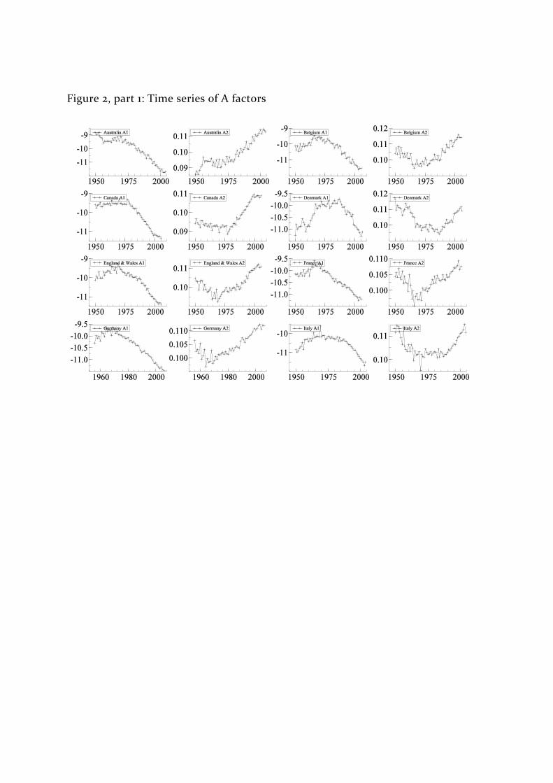
Figure 2, part 1: Time series of A factors

Figure 2, part 2: Time series of A factors

Figure 3: Cross plots of A factors

Figure 4: Density Plots of Annuity Valuation with ( ) 0- =Irank p , parameters
certain (solid line) and uncertain (dotted line).
Figure 5: Density Plots of Annuity Valuation with ( ) 1- =Irank p , parameters
certain (solid line) and uncertain (dotted line).

Figure 6: Density Plots of Annuity Valuation with ( ) 2- =Irank p , parameters
certain (solid line) and uncertain (dotted line).


Table 1: Unit Root Tests on Estimated Factors
Analysis of 1ˆtA Analysis of 2ˆ
tA
DF test Measurement error DF test Measurement error
[conventional p‐value] p‐value power [conventional p‐value] p‐value power
Australia ‐4.62 [0.01] 0.02 0.95 ‐5.36 [0.00] 0.00 0.99
Belgium ‐4.49 [0.01] 0.03 0.91 ‐4.65 [0.01] 0.02 0.96
Canada ‐2.42 [0.36] 0.99 1.00 ‐1.88 [0.63] 0.94 0.04
Denmark ‐3.06 [0.14] 0.87 1.00 ‐3.42 [0.07] 0.54 1.00
England & Wales ‐2.74 [0.24] 0.56 0.32 ‐3.25 [0.10] 0.20 0.71
France ‐3.95 [0.03] ‐4.35 [0.01]
Germany ‐3.57 [0.05] ‐4.46 [0.01]
Italy ‐2.70 [0.25] 0.95 1.00 ‐3.16 [0.12] 0.37 0.45
Japan ‐2.73 [0.24] ‐4.29 [0.01] 0.44 1.00
Netherlands ‐3.17 [0.11] 0.47 0.27 ‐4.72 [0.01] 0.03 0.86
Norway ‐1.88 [0.63] 0.76 0.19 ‐2.09 [0.52] 0.64 0.30
Poland ‐3.37 [0.08] ‐3.43 [0.07] 0.88 1.00
Spain ‐3.68 [0.04] ‐4.36 [0.01] 0.16 1.00
Sweden ‐4.35 [0.01] 0.80 1.00 ‐5.11 [0.00] 0.05 1.00
Switzerland ‐3.30 [0.09] ‐3.60 [0.05]
USA 0.99 [1.00] 0.79 [1.00]

Table 2: Annuity valuation under different models of the factors
Australia Belgium Canada Denmark Eng & Wales France Germany Italy
Cert Unc Cert Unc Cert Unc Cert Unc Cert Unc Cert Unc Cert Unc Cert Unc
Rank 2 (equation 7)
Expected value 16.36 16.49 14.85 14.85 15.96 16.44 14.53 14.76 15.61 15.68 15.65 15.68 15.84 16.30 15.63 15.62
Lower decile 16.29 16.04 14.83 14.76 15.86 15.43 14.42 14.11 15.55 15.36 15.62 15.51 15.73 15.31 15.60 15.48
Upper decile 16.43 17.00 14.87 14.94 16.06 18.48 14.65 15.54 15.66 16.07 15.68 15.85 15.95 18.24 15.66 15.78
90:10 range 0.14 0.96 0.05 0.18 0.19 3.05 0.23 1.43 0.11 0.71 0.06 0.34 0.22 2.93 0.05 0.30
Rank 1 (equation 8)
Expected value 16.20 16.20 14.81 14.81 15.90 15.88 14.18 14.18 15.35 15.35 15.67 15.67 15.26 15.26 15.47 15.49
Lower decile 15.97 15.86 14.57 14.47 15.72 15.60 13.87 13.73 15.18 15.11 15.49 15.40 15.10 15.04 15.29 15.21
Upper decile 16.43 16.53 15.06 15.15 16.08 16.16 14.49 14.62 15.51 15.58 15.86 15.94 15.41 15.48 15.65 15.79
90:10 range 0.46 0.67 0.49 0.68 0.37 0.56 0.62 0.89 0.33 0.47 0.37 0.54 0.30 0.44 0.35 0.58
Rank 0 (equation 6)
Expected value 16.32 16.35 14.95 14.97 15.56 15.56 14.46 14.47 15.54 15.55 15.66 15.67 15.37 15.38 15.95 15.97
Lower decile 15.58 15.26 14.47 14.28 15.25 15.11 14.01 13.84 15.04 14.83 15.19 14.97 15.02 14.86 15.36 15.10
Upper decile 17.09 17.49 15.44 15.72 15.87 16.03 14.91 15.11 16.04 16.31 16.14 16.38 15.73 15.90 16.56 16.87
90:10 range 1.51 2.23 0.98 1.44 0.62 0.92 0.89 1.27 1.00 1.48 0.96 1.41 0.71 1.04 1.19 1.78
"Spread" 1.0% 1.8% 0.9% 1.1% 2.5% 5.5% 2.4% 4.0% 1.7% 2.2% 0.1% 0.1% 3.8% 6.7% 3.1% 3.0%
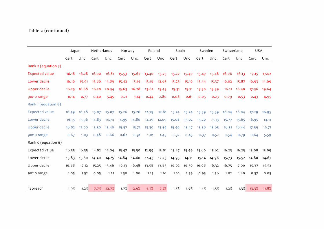
Table 2 (continued)
Japan Netherlands Norway Poland Spain Sweden Switzerland USA
Cert Unc Cert Unc Cert Unc Cert Unc Cert Unc Cert Unc Cert Unc Cert Unc
Rank 2 (equation 7)
Expected value 16.18 16.28 16.00 16.81 15.53 15.67 13.40 13.75 15.27 15.40 15.47 15.48 16.06 16.13 17.15 17.02
Lower decile 16.10 15.91 15.80 14.89 15.42 15.14 13.18 12.63 15.23 15.10 15.44 15.37 16.02 15.87 16.93 14.69
Upper decile 16.25 16.68 16.20 20.34 15.63 16.28 13.62 15.43 15.31 15.71 15.50 15.59 16.11 16.40 17.36 19.64
90:10 range 0.14 0.77 0.40 5.45 0.21 1.14 0.44 2.80 0.08 0.61 0.05 0.23 0.09 0.53 0.43 4.95
Rank 1 (equation 8)
Expected value 16.49 16.48 15.07 15.07 15.26 15.26 12.79 12.81 15.24 15.24 15.39 15.39 16.04 16.04 17.29 16.95
Lower decile 16.15 15.96 14.83 14.74 14.95 14.80 12.29 12.09 15.08 15.02 15.20 15.13 15.77 15.65 16.95 14.11
Upper decile 16.82 17.00 15.30 15.40 15.57 15.71 13.30 13.54 15.40 15.47 15.58 15.65 16.31 16.44 17.59 19.71
90:10 range 0.67 1.03 0.48 0.66 0.62 0.91 1.01 1.45 0.32 0.45 0.37 0.52 0.54 0.79 0.64 5.59
Rank 0 (equation 6)
Expected value 16.35 16.35 14.82 14.84 15.47 15.50 12.99 13.01 15.47 15.49 15.60 15.62 16.23 16.25 15.08 15.09
Lower decile 15.83 15.60 14.40 14.25 14.84 14.60 12.43 12.23 14.93 14.71 15.14 14.96 15.73 15.52 14.80 14.67
Upper decile 16.88 17.12 15.25 15.46 16.13 16.48 13.58 13.83 16.02 16.30 16.08 16.32 16.75 17.00 15.37 15.52
90:10 range 1.05 1.52 0.85 1.21 1.30 1.88 1.15 1.61 1.10 1.59 0.93 1.36 1.02 1.48 0.57 0.85
"Spread" 1.9% 1.2% 7.7% 12.7% 1.7% 2.6% 4.7% 7.2% 1.5% 1.6% 1.4% 1.5% 1.2% 1.3% 13.3% 11.8%

Table 3: Consequences for the money’s worth (parameters uncertain)
Rank 2 (equation 7)
Rank 1 (equation 8)
Rank 0 (equation 6)
Australia 0.970 0.980 0.935
Belgium 0.994 0.978 0.953
Canada 0.890 0.982 0.971
Denmark 0.950 0.970 0.957
Eng & Wales 0.976 0.985 0.954
France 0.989 0.983 0.956
Germany 0.894 0.986 0.967
Italy 0.990 0.981 0.946
Japan 0.976 0.970 0.955
Netherlands 0.827 0.978 0.960
Norway 0.962 0.971 0.941
Poland 0.892 0.946 0.940
Spain 0.980 0.985 0.950
Sweden 0.993 0.983 0.957
Switzerland 0.984 0.976 0.956
USA 0.867 0.860 0.972

Table 4: The effect of incorporating factor measurement error into projections
Ignoring measurement error in factors Modelling measurement error in factors
Netherlands
Mean 14.838 14.836
Lower decile 14.257 14.276
Upper decile 15.450 15.414
90:10 1.192 1.138
Money's worth 0.960 0.962
Norway
Mean 15.505 15.509
Lower decile 14.611 14.648
Upper decile 16.462 16.446
90:10 1.851 1.798
Money's worth 0.942 0.943