Proceedings: Building Simulation 2007

- 1150 -

DISCUSSION ON GRID SIZE AND COMPUTATION DOMAIN IN CFD SIMULATION OF PEDESTRIAN WIND ENVIRONMENT AROUND BUILDINGS

Wei Zhong Xiang1 and Hua Sheng Wang2

1Hoare Lea Consulting Engineers, Royal Exchange, Cross Street, Manchester, M2 7FL, UK.

Tel: +44 1612141406, email: weizhongxiang@ve.hoarelea.com 2School of Engineering and Materials Science, Queen Mary, University of London, Mile End

Road, London E1 4NS, UK. Tel: +44 2078829721, email: h.s.wang@qmul.ac.uk

ABSTRACT With the rapid development of computers and CFD, pedestrian level wind study using CFD has become important in engineering design in recent years. In the United Kingdom, wind study is now a common engineering practice and a mandatory documentation for plan authority. The paper presents preliminary CFD simulation of pedestrian wind environment around buildings of typical configuration, size and orientation. The results were compared for flow pattern and the wind velocity amplification value at the pedestrian level, a horizontal surface 1.5 m above ground. The grid size and computation domain independent results were obtained when the grid size in the pedestrian level is less than 1.0 m and the computation domain dimensions are greater than five times the height of buildings under the conditions.

KEYWORDS Wind study, CFD, Grid size, Computation domain

INTRODUCTION The wind environment around buildings is determined by many factors such as the configuration, size and orientation of buildings. Buildings and channels formed between buildings can produce high wind velocity at the pedestrian level, the area below 2.0 m above ground. The wind environment can be measured by a reduced size model in wind tunnel or obtained by CFD simulation. With the rapid development of computers and CFD, wind study using CFD has been important in engineering design in recent years since it is cheaper, less time consuming and able to give detailed information as needed. In the United Kingdom, wind study is now a common engineering practice and a mandatory documentation for plan authority. A method for wind study is given in BRE digest 390 (BRE digest 390) of the Building Research Establishment of the UK and in (Lawson 2001, Blocken 2004). The wind flow patterns around buildings are determined for eight wind directions using the annual average wind velocity as a reference. The local wind velocity is expressed as a ratio of the predicted velocity, U, to the free wind velocity, UF, at

the same height if no tall building or obstruction was present, given by Eq.(1).

FUUR = (1)

The results are combined with the wind data statistics to assess how often certain wind velocities are exceeded annually. The aim of wind study is, therefore, to determine the R values in the pedestrian level. Since the height of the pedestrian level is very much smaller than the height of tall buildings and hence the height of the computation domain (also referred to as virtual wind tunnel, VWT), proper selection of the grid size and computation domain is crucial in order to obtain independent, reliable results within the limitation of computer resources. Woolhouse (Woolhouse 2006) suggests the computation domain is determined by a blockage factor of 3%, which is defined as the ratio of the upwind building face area of buildings to the corresponding area of the computation domain, when the height and side spacing are equal, and the downward boundary distance in the range of 10 to 30 times the height. This method generally gives a bigger computation domain. For the buildings specified in Fig. 1 below, for example, the computation domain is 6.4 times the height of buildings, H. ASHRAE (ASHRAE Handbook 2001) recommends that the flow pattern is not affected by the buildings when the distance from the roof is equal or greater than 1.5S. The scaling length, S, is calculated by Eq. (2)

33.0L

67.0S BBS = (2)

where SB and LB are the smaller and larger of upwind building face dimensions, width W and height H, respectively. When LB is larger than S8B , take

sL 8BB = . The ASHRAE (ASHRAE Handbook 2001) method generally gives a much smaller computation domain. For the buildings specified in Fig. 1 below, for example, the computation domain is 1.8 times the height of buildings, H. The present paper conducts preliminary simulation for a typical building configuration, size

Proceedings: Building Simulation 2007

- 1151 -

and orientation to exam the effects of the grid size and computation domain.

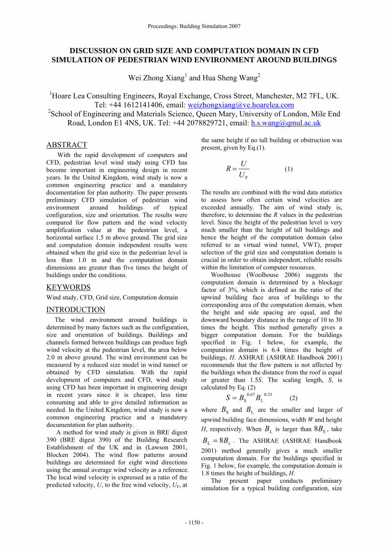
COMPUTATIONAL MODEL AND BOUNDARY CONDITIONS Figure 1 shows the computational model, coordinates for a typical configuration, size and orientation of the buildings. Four identical buildings with width W, height H and depth D are located with distances S1 and S2 in both X and Y directions. For the purpose of the present study, dimensions of W, H,

and D are taken to be 50, 30 and 20 m, respectively, and S1 and S2 30 and 15 m, respectively. The wind is coming from the direction as shown in Fig. 1. Due to the symmetry the right hand side half is chosen to be the computation domain as shown by the dashed lines in Fig. 1. The windward, sideward, leeward and height (not shown in Fig. 1) of the computation domain are denoted as LW, LS, LL, LH, respectively. X and Y coordinates are set on the ground, traverse to and along the wind direction, respectively. Z (not shown in Fig.1) coordinate is vertically upwards from the ground.

Figure 1 Computation model and coordinates The RNG k-ε turbulence model was used. Following Hu and Wang(Hu 2005), the turbulent kinetic energy k and dissipation rate ε are calculated by Eqs. (3) and (4).

C

uk′

= (3)

( )

zu

z κε

3′= (4)

where u′ is friction velocity, κ (=0.41) is the von Kaman constant and C = 0.09. The approach wind velocity profile at the boundary AW was calculated by Eq. (5) (ASHRAE (ASHRAE Handbook 2001))

αα

⎟⎠⎞

⎜⎝⎛

⎟⎟⎠

⎞⎜⎜⎝

⎛=

hz

zh

UU z

met

met

metmet (5)

where Umet is the wind velocity measured at the meteorological station, zmet is the height of the anemometer at the meteorological station (normal value is 10m), z is the height, h is the boundary layer thickness, α is the exponent, αmet and hmet are the values of α and h at the meteorological station. The values of α and h are taken as follows (details see ASHRAE (ASHRAE Handbook 2001), 16.3): for large city α = 0.33, h = 460 m; urban and suburban α = 0.22, h = 370 m; open terrain α = 0.14, h = 270 m; flat unobstructed areas α = 0.1, h = 210 m. In the present study, urban and suburban wind profile was used and the Umet was taken to be 4.0 m/s (CIBSE Guide 2002). It is noted that the free wind velocity used in Eq. (1) is obtained by Eq. (5). The boundary condition at the leeward AL was assumed to be a pressure outlet. The boundary conditions at the centre surface AC, sideward AS and top (not shown) were assumed to be symmetric condition. Standard wall function was used for the ground and building walls. The turbulent kinetic energy k at the boundaries is calculated by Eq. (6).

AL

Computation domain, VWT

W S1

LSL W

L L

D

S 2

Wind direction AW

AS

AC

X

Y

Proceedings: Building Simulation 2007

- 1152 -

( )2

23 IUk zz = (6)

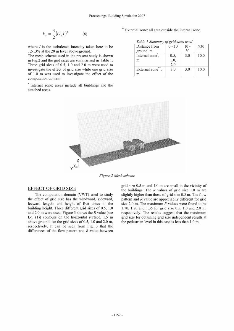
where I is the turbulence intensity taken here to be 12-13% at the 20 m level above ground. The mesh scheme used in the present study is shown in Fig.2 and the grid sizes are summarised in Table 1. Three grid sizes of 0.5, 1.0 and 2.0 m were used to investigate the effect of grid size while one grid size of 1.0 m was used to investigate the effect of the computation domain. * Internal zone: areas include all buildings and the attached areas.

** External zone: all area outside the internal zone.

Table 1 Summary of grid sizes used Distance from ground, m

0 - 10 10 - 30

≥30

Internal zone*, m

0.5, 1.0, 2.0

3.0 10.0

External zone**, m

3.0 3.0 10.0

Figure 2 Mesh scheme

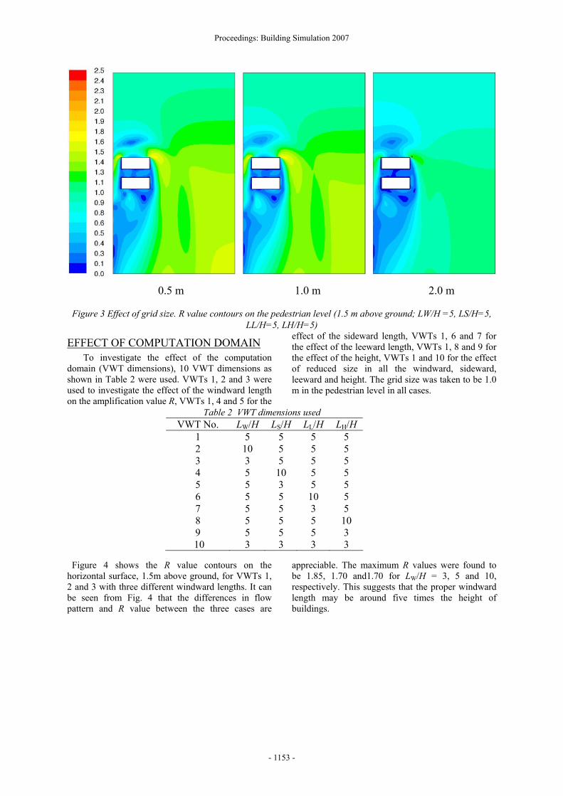
EFFECT OF GRID SIZE The computation domain (VWT) used to study the effect of grid size has the windward, sideward, leeward lengths and height of five times of the building height. Three different grid sizes of 0.5, 1.0 and 2.0 m were used. Figure 3 shows the R value (see Eq. (1)) contours on the horizontal surface, 1.5 m above ground, for the grid sizes of 0.5, 1.0 and 2.0 m, respectively. It can be seen from Fig. 3 that the differences of the flow pattern and R value between

grid size 0.5 m and 1.0 m are small in the vicinity of the buildings. The R values of grid size 1.0 m are slightly higher than those of grid size 0.5 m. The flow pattern and R value are appreciablly different for grid size 2.0 m. The maximum R values were found to be 1.70, 1.70 and 1.35 for grid size 0.5, 1.0 and 2.0 m, respectively. The results suggest that the maximum grid size for obtaining grid size independent results at the pedestrian level in this case is less than 1.0 m.

Proceedings: Building Simulation 2007

- 1153 -

0.5 m 1.0 m 2.0 m

Figure 3 Effect of grid size. R value contours on the pedestrian level (1.5 m above ground; LW/H =5, LS/H=5, LL/H=5, LH/H=5)

EFFECT OF COMPUTATION DOMAIN To investigate the effect of the computation domain (VWT dimensions), 10 VWT dimensions as shown in Table 2 were used. VWTs 1, 2 and 3 were used to investigate the effect of the windward length on the amplification value R, VWTs 1, 4 and 5 for the

effect of the sideward length, VWTs 1, 6 and 7 for the effect of the leeward length, VWTs 1, 8 and 9 for the effect of the height, VWTs 1 and 10 for the effect of reduced size in all the windward, sideward, leeward and height. The grid size was taken to be 1.0 m in the pedestrian level in all cases.

Table 2 VWT dimensions used VWT No. LW/H LS/H LL/H LH/H

1 5 5 5 5 2 10 5 5 5 3 3 5 5 5 4 5 10 5 5 5 5 3 5 5 6 5 5 10 5 7 5 5 3 5 8 5 5 5 10 9 5 5 5 3

10 3 3 3 3 Figure 4 shows the R value contours on the horizontal surface, 1.5m above ground, for VWTs 1, 2 and 3 with three different windward lengths. It can be seen from Fig. 4 that the differences in flow pattern and R value between the three cases are

appreciable. The maximum R values were found to be 1.85, 1.70 and1.70 for LW/H = 3, 5 and 10, respectively. This suggests that the proper windward length may be around five times the height of buildings.

Proceedings: Building Simulation 2007

- 1154 -

LW/H = 3 LW/H = 5 LW/H = 10

Figure 4 Effect of windward length. R value contours on the pedestrian level (1.5 m above ground; LS/H=5, LL/H=5, LH/H=5)

Figure 5 shows the R value contours on the horizontal surface, 1.5m above ground, for VWTs 1, 4 and 5 with three different sideward lengths. It can be seen from Fig. 5 that the differences in flow pattern and R value between the three cases are small.

The maximum R values were found to be 1.85, 1.70 and1.70 for LS/H = 3, 5 and 10, respectively. This suggests that the computation domain with the sideward length greater than five times the height of buildings is needed.

LS/H = 3 LS/H = 5 LS/H = 10

Figure 5 Effect of sideward length. R value contours on the pedestrian level (1.5 m above ground; LW/H=5, LL/H=5, LH/H=5)

Figure 6 shows the R value contours on the horizontal surface, 1.5m above ground, for VWTs 1, 6 and 7 with three different leeward lengths. It can be seen from Fig. 6 that the differences in flow pattern and R value between the three cases are small.

The maximum R values were found to be 1.70, 1.70 and1.70 for LS/H = 3, 5 and 10, respectively. This suggests that the leeward length may be reduced to three times the height of buildings.

Proceedings: Building Simulation 2007

- 1155 -

LL/H = 3 LL/H = 5 LL/H = 10

Figure 6 Effect of leeward length. R value contours on the pedestrian level (1.5 m above ground; LW/H=5, LS/H=5, LH/H=5)

Figure 7 shows the R value contours on the horizontal surface, 1.5m above ground, for VWTs 1, 8 and 9 with three different heights. It can be seen from Fig. 7 that the differences in flow pattern and R value between the three cases are small. The

maximum R values were found to be 1.85, 1.70 and1.70 for LH/H = 3, 5 and 10, respectively. This suggests that the height of the computation domain may be reduced to five times the height of buildings.

LH/H = 3 LH/H = 5 LH/H = 10

Figure 7 Effect of height. R value contours on the pedestrian level (1.5 m above ground; LW/H=5, LS/H=5, LL/H=5)

Figure 8 shows the R value contours on the horizontal surface, 1.5m above ground, for VWT1 and 10 with all dimensions in windward, sideward, leeward and height 3 and 5 times the height of buildings,

respectively. It can be seen from Fig. 8 that the differences in flow pattern and R value between the two cases are significant. The maximum R values were found to be 1.95 and 1.70 for VWT1 and

Proceedings: Building Simulation 2007

- 1156 -

VWT10, respectively. This suggests that the dimensions of the computation domain in all

directions cannot be reduced simultaneously to less than five times the height of buildings.

LW/H = LS/H = LL/H = LH/H= 3 LW/H = LS/H= LL/H = LH/H = 5

Figure 8 Effect of computation domain. R value contours on the pedestrian level (1.5 m above ground)

CONCLUSION The results would not be expected to be true outside the particular conditions used here. In order to obtain useful, general results on the grid size and computation domain for buildings of various configurations, sizes, and orientations, much more detailed simulations are needed.

REFERENCES BRE digest 390, “Wind around tall buildings” Lawson T. 2001, Building Aerodynamics, Imperial

College Press. Blocken B. 2004, “Pedestrian wind environment

around buildings: literature review and practical examples,” Journal of Thermal Env. & Bldg. Sci., 28 (2): 107-159.

Hu. H and Wang. F. 2005, “Using a CFD approach for the study of street-level winds in a built-up area,” Building and Environment, 40: 617-631.

CIBSE Guide J. 2002, Weather, Solar and Luminance Data.

Woolhouse R. 2006, “Modelling Environmental Airflow”, User Group Meeting Ansys Fluent, 21-22 September, Nottingham, UK.

ASHRAE Handbook - Fundamental, 2001.