Data Mining and Knowledge Discovery, 6, 393–423, 2002c© 2002 Kluwer Academic Publishers. Manufactured in The Netherlands.

Discretization: An Enabling Technique

HUAN LIU hliu@asu.eduFARHAD HUSSAIN farhad@comp.nus.edu.sgCHEW LIM TAN tancl@comp.nus.edu.sgMANORANJAN DASH manoranj@comp.nus.edu.sgSchool of Computing, National University of Singapore, Singapore

Editors: Fayyad, Mannila, Ramakrishnan

Received June 29, 1999; Revised July 12, 2000

Abstract. Discrete values have important roles in data mining and knowledge discovery. They are about intervalsof numbers which are more concise to represent and specify, easier to use and comprehend as they are closer toa knowledge-level representation than continuous values. Many studies show induction tasks can benefit fromdiscretization: rules with discrete values are normally shorter and more understandable and discretization canlead to improved predictive accuracy. Furthermore, many induction algorithms found in the literature requirediscrete features. All these prompt researchers and practitioners to discretize continuous features before or duringa machine learning or data mining task. There are numerous discretization methods available in the literature. It istime for us to examine these seemingly different methods for discretization and find out how different they reallyare, what are the key components of a discretization process, how we can improve the current level of research fornew development as well as the use of existing methods. This paper aims at a systematic study of discretizationmethods with their history of development, effect on classification, and trade-off between speed and accuracy.Contributions of this paper are an abstract description summarizing existing discretization methods, a hierarchicalframework to categorize the existing methods and pave the way for further development, concise discussions ofrepresentative discretization methods, extensive experiments and their analysis, and some guidelines as to how tochoose a discretization method under various circumstances. We also identify some issues yet to solve and futureresearch for discretization.

Keywords: discretization, continuous feature, data mining, classification

1. Introduction

Data usually comes in a mixed format: nominal, discrete, and/or continuous. Discrete andcontinuous data are ordinal data types with orders among the values, while nominal values donot possess any order amongst them. Discrete values are intervals in a continuous spectrumof values. While the number of continuous values for an attribute can be infinitely many, thenumber of discrete values is often few or finite. The two types of values make a differencein learning classification trees/rules. One example of decision tree induction can furtherillustrate the difference between the two data types. When a decision tree is induced, onefeature is chosen to branch on its values. With the coexistence of continuous and discretefeatures, normally, a continuous feature will be chosen as it has more values than features ofother types do. By choosing a continuous feature, the next level of a tree can quickly reach a

394 LIU ET AL.

“pure” state—with all instances in a child/leaf node belonging to one class. In many cases,this is tantamount to a table-lookup along one dimension which leads to poor performanceof a classifier. Therefore it is certainly not wise to use continuous values to split a node.There is a need to discretize continuous features either before the decision tree induction orduring the process of tree building. Widely used systems such as C4.5 (Quinlan, 1993) andCART (Breiman et al., 1984) deploy various ways to avoid using continuous values directly.There are many other advantages of using discrete values over continuous ones. Discretefeatures are closer to a knowledge-level representation (Simon, 1981) than continuous ones.Data can also be reduced and simplified through discretization. For both users and experts,discrete features are easier to understand, use, and explain. As reported in a study (Doughertyet al., 1995), discretization makes learning more accurate and faster. In general, obtainedresults (decision trees, induction rules) using discrete features are usually more compact,shorter and more accurate than using continuous ones, hence the results can be more closelyexamined, compared, used and reused. In addition to the many advantages of having discretedata over continuous one, a suite of classification learning algorithms can only deal withdiscrete data. Discretization is a process of quantizing continuous attributes. The successof discretization can significantly extend the borders of many learning algorithms.

This paper is about reviewing existing discretization methods, standardizing the dis-cretization process, summarizing them with an abstract framework, providing a convenientreference for future research and development. The remainder of the paper is organizedas follows. In the next section, we summarize the current status of discretization methods.In Section 3, we provide a unified vocabulary for discussing various methods introducedby many authors, define a general process of discretization, and discuss different ways ofevaluating discretization results. In Section 4, we propose a new hierarchical frameworkfor discretization methods; describe representative methods concisely; while describinga representative method, we also provide its discretization results for a commonly usedbenchmark data set (Iris). Section 5 shows the results of comparative experiments amongvarious methods and some analysis. The paper concludes in Section 6 with guidelines ofchoosing a discretization method and further work.

2. Current status

In earlier days simple techniques were used such as equal-width and equal-frequency (or, aform of binning) to discretize. As the need for accurate and efficient classification grew, thetechnology for discretization develops rapidly. Over the years, many discretization algo-rithms have been proposed and tested to show that discretization has the potential to reducethe amount of data while retaining or even improving predictive accuracy. Discretizationmethods have been developed along different lines due to different needs: supervised vs.unsupervised, dynamic vs. static, global vs. local, splitting (top-down) vs. merging (bottom-up), and direct vs. incremental.

As we know, data can be supervised or unsupervised depending on whether it has classinformation. Likewise, supervised discretization considers class information while unsu-pervised discretization does not; unsupervised discretization is seen in earlier methodslike equal-width and equal-frequency. In the unsupervised methods, continuous ranges are

DISCRETIZATION 395

divided into subranges by the user specified width (range of values) or frequency (numberof instances in each interval). This may not give good results in cases where the distributionof the continuous values is not uniform. Furthermore it is vulnerable to outliers as theyaffect the ranges significantly (Catlett, 1991). To overcome this shortcoming, superviseddiscretization methods were introduced and class information is used to find the proper inter-vals caused by cut-points. Different methods have been devised to use this class informationfor finding meaningful intervals in continuous attributes.

Supervised and unsupervised discretization have their different uses. If no class infor-mation is available, unsupervised discretization is the sole choice. There are not manyunsupervised methods available in the literature which may be attributed to the fact thatdiscretization is commonly associated with the classification task. One can also view theusage of discretization methods as dynamic or static. A dynamic method would discretizecontinuous values when a classifier is being built, such as in C4.5 (Quinlan, 1993) while inthe static approach discretization is done prior to the classification task. There is a compar-ison between dynamic and static methods in Dougherty et al. (1995). The authors reportedmixed performance when C4.5 was tested with and without discretized features (static vs.dynamic).

Another dichotomy is local vs. global. A local method would discretize in a localizedregion of the instance space (i.e. a subset of instances) while a global discretization methoduses the entire instance space to discretize (Chmielewski and Grzymala-Busse, 1994). So,a local method is usually associated with a dynamic discretization method in which only aregion of instance space is used for discretization.

Discretization methods can also be grouped in terms of top-down or bottom-up. Top-downmethods start with an empty list of cut-points (or split-points) and keep on adding new onesto the list by ‘splitting’ intervals as the discretization progresses. Bottom-up methods startwith the complete list of all the continuous values of the feature as cut-points and removesome of them by ‘merging’ intervals as the discretization progresses.

Another dimension of discretization methods is direct vs. incremental. Direct methods di-vide the range of k intervals simultaneously (i.e., equal-width and equal-frequency), needingan additional input from the user to determine the number of intervals. Incremental methodsbegin with a simple discretization and pass through an improvement process, needing anadditional criterion to know when to stop discretizing (Cerquides and Mantaras, 1997).

As shown above, there are numerous discretization methods and many different dimen-sions to group them. A user of discretization often finds it difficult to choose a suitablemethod for the data on hand. There have been a few attempts (Dougherty et al., 1995;Cerquides and Mantaras, 1997) to help alleviate the difficulty. We carry on with this keyobjective to make a comprehensive study that includes the definition of a discretizationprocess, performance measures, and extensive comparison. Contributions of this workare:

1. An abstract description of a typical discretization process,2. A new hierarchical framework to categorize existing discretization methods in the

literature,3. A systematic demonstration of different results by various discretization methods using

a benchmark data set,

396 LIU ET AL.

4. A comparison of nine representative discretization methods chosen from the frameworkalong two dimensions: times and error rates of a learning algorithm for classificationover publically available benchmark data sets,

5. Detailed examination of comparative results, and6. Some guidelines as to which method to use under different circumstances, and directions

for future research and development.

3. Discretization process

We first clarify some terms used in different works followed by an abstract description ofa typical discretization process.

3.1. Terms and notations

3.1.1. Feature. “Feature” or “Attribute” or “Variable” refers to an aspect of the data.Usually before collecting data, features are specified or chosen. Features can be discrete,continuous, or nominal. In this paper we are interested in the process of discretizing con-tinuous features. Hereafter M stands for the number of features in the data.

3.1.2. Instance. “Instance” or “Tuple” or “Record” or “Data point” refers to a singlecollection of feature values for all features. A set of instances makes a data set. Usually adata set is in a matrix form where a row corresponds to an instance and a column correspondsto a feature. Hereafter N is the number of instances in the data.

3.1.3. Cut-point. The term “cut-point” refers to a real value within the range of continuousvalues that divides the range into two intervals, one interval is less than or equal to the cut-point and the other interval is greater than the cut-point. For example, a continuous interval[a, b] is partitioned into [a, c] and (c, b], where the value c is a cut-point. Cut-point is alsoknown as split-point.

3.1.4. Arity. The term “arity” in the discretization context means the number of intervals orpartitions. Before discretization of a continuous feature, arity can be set to k—the numberof partitions in the continuous features. The maximum number of cut-points is k − 1.Discretization process reduces the arity but there is a trade-off between arity and its effecton the accuracy of classification and other tasks. A higher arity can make the understandingof an attribute more difficult while a very low arity may affect predictive accuracy negatively.

3.2. A typical discretization process

By “typical” we mean univariate discretization. Discretization can be univariate or multi-variate. Univariate discretization quantifies one continuous feature at a time while multivari-ate discretization considers simultaneously multiple features. We mainly consider univari-ate discretization throughout this paper and discuss more about multivariate discretizationbriefly at the end as an extension of univariate discretization.

DISCRETIZATION 397

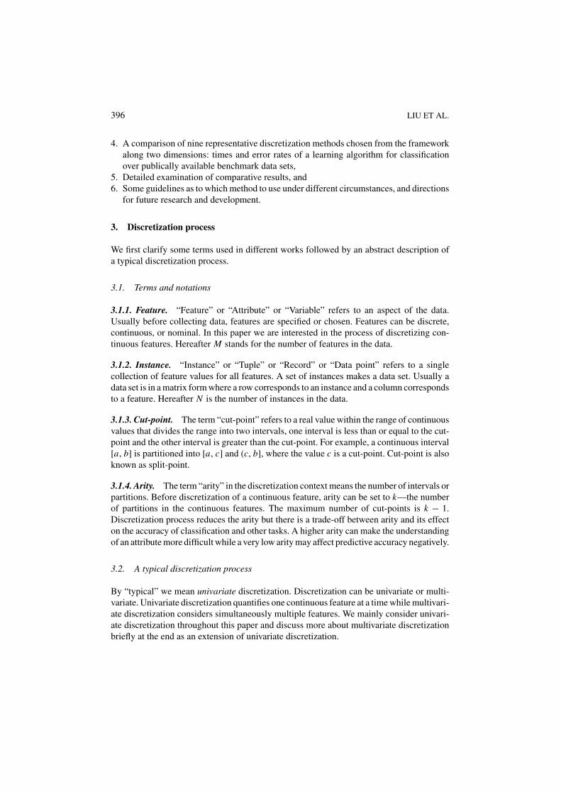
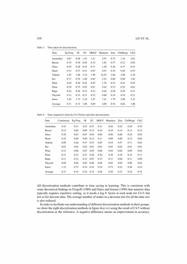
Figure 1. Discretization process.

A typical discretization process broadly consists of four steps (seen in figure 1): (1) sortingthe continuous values of the feature to be discretized, (2) evaluating a cut-point for splittingor adjacent intervals for merging, (3) according to some criterion, splitting or mergingintervals of continuous value, and (4) finally stopping at some point. In the following wediscuss these four steps in more detail.

3.2.1. Sorting. The continuous values for a feature is sorted in either descending or ascend-ing order. Sorting can be computationally very expensive if care is not taken in implementingit with discretization. It is important to speed up the discretization process by selecting suit-able sorting algorithms. Many sorting algorithms can be found in classic data structures andalgorithms books. Among these “Quick-sort” is an efficient sorting algorithm with a timecomplexity of O(N log N ).

Another way to improve efficiency is to avoid sorting a feature’s values repeatedly. Ifsorting is done once and for all at the beginning of discretization, it is a global treatmentand can be applied when the entire instance space is used for discretization. If sorting isdone at each iteration of a process, it is a local treatment in which only a region of entireinstance space is considered for discretization.

3.2.2. Choosing a cut-point. After sorting, the next step in the discretization process is tofind the best “cut-point” to split a range of continuous values or the best pair of adjacent

398 LIU ET AL.

intervals to merge. One typical evaluation function is to determine the correlation of asplit or a merge with the class label. There are numerous evaluation functions found in theliterature such as entropy measures and statistical measures. More about these evaluationfunctions and their various applications is discussed in the following sections.

3.2.3. Splitting/merging. As we know, in a top-down approach, intervals are split whilefor a bottom-up approach intervals are merged. For splitting it is required to evaluate ‘cut-points’ and to choose the best one and split the range of continuous values into two partitions.Discretization continues with each part (increased by one) until a stopping criterion issatisfied. Similarly for merging, adjacent intervals are evaluated to find the best pair ofintervals to merge in each iteration. Discretization continues with the reduced number(decreased by one) of intervals until the stopping criterion is satisfied.

3.2.4. Stopping criteria. A stopping criterion specifies when to stop the discretizationprocess. It is usually governed by a trade-off between lower arity with a better understandingbut less accuracy and a higher arity with a poorer understanding but higher accuracy. Wemay consider k to be an upper bound for the arity of the resulting discretization. In practicethe upper bound k is set much less than N , assuming there is no repetition of continuousvalue for a feature. A stopping criterion can be very simple such as fixing the number ofintervals at the beginning or a more complex one like evaluating a function. We describedifferent stopping criteria in the next section.

3.3. Result evaluation for discretization

Assuming we have many methods and each provides some kind of discretized data, whichdiscretized data is the best? This seemingly simple question cannot be easily dealt with asimple answer. This is because the result evaluation is a complex issue and depends on auser’s need in a particular application. It is complex because the evaluation can be done inmany ways. We list three important dimensions: (1) The total number of intervals—intuitively, the fewer the cut-points, the better the discretization result; but there is a limitimposed by the data representation. This leads to the next dimension. (2) The numberof inconsistencies (inconsistency is defined later) caused by discretization—it should notbe much higher than the number of inconsistencies of the original data before discretization.If the ultimate goal is to generate a classifier from the data, we should consider yet anotherperspective. (3) Predictive accuracy—how discretization helps improve accuracy. In short,we need at least three dimensions: simplicity, consistency, and accuracy. Ideally, the bestdiscretization result can score highest in all three departments. In reality, it may not beachievable, or necessary. To provide a balanced view of various discretization methods interms of these measures is one of the objectives of this paper.

Simplicity is defined by the total number of cut-points. Accuracy is usually obtainedby running classifier in cross validation mode. Consistency is defined by having the leastinconsistency count which is calculated in three steps: (in the following description a patternis a set of values for a feature set while an instance is a pattern with a class label) (1) twoinstances are considered inconsistent if they are the same in their attribute values except for

DISCRETIZATION 399

their class labels; for example, we have an inconsistency if there are two instances (0 1, a)and (0 1, a)—class label is separated by “,”—because of different classes a and a. (2) theinconsistency count for a pattern is the number of times it appears in the data minus thelargest number of class label: for example, let us assume there are n instances that matchthe pattern, among them, c1 instances belong to label1, c2 to label2, and c3 to label3 wherec1 + c2 + c3 = n. If c3 is the largest among the three, the inconsistency count is (n − c3).(3) the total inconsistency count is the sum of all the inconsistency counts for all possiblepatterns of a feature subset.

4. Discretization framework

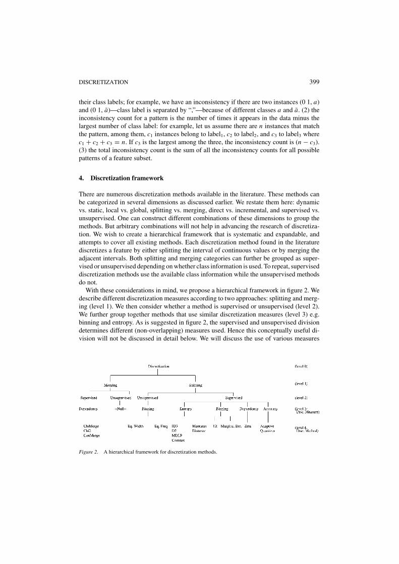
There are numerous discretization methods available in the literature. These methods canbe categorized in several dimensions as discussed earlier. We restate them here: dynamicvs. static, local vs. global, splitting vs. merging, direct vs. incremental, and supervised vs.unsupervised. One can construct different combinations of these dimensions to group themethods. But arbitrary combinations will not help in advancing the research of discretiza-tion. We wish to create a hierarchical framework that is systematic and expandable, andattempts to cover all existing methods. Each discretization method found in the literaturediscretizes a feature by either splitting the interval of continuous values or by merging theadjacent intervals. Both splitting and merging categories can further be grouped as super-vised or unsupervised depending on whether class information is used. To repeat, superviseddiscretization methods use the available class information while the unsupervised methodsdo not.

With these considerations in mind, we propose a hierarchical framework in figure 2. Wedescribe different discretization measures according to two approaches: splitting and merg-ing (level 1). We then consider whether a method is supervised or unsupervised (level 2).We further group together methods that use similar discretization measures (level 3) e.g.binning and entropy. As is suggested in figure 2, the supervised and unsupervised divisiondetermines different (non-overlapping) measures used. Hence this conceptually useful di-vision will not be discussed in detail below. We will discuss the use of various measures

Figure 2. A hierarchical framework for discretization methods.

400 LIU ET AL.

under the categories of splitting and merging as shown in the table below (X indicatesthat a measure is not available in the category. We may find variations of these measureslike Mantaras distance (Cerquides and Mantaras, 1997) which we categorize under entropymeasure for their similarity.)

Splitting Merging

Binning X

Entropy X

Dependency Dependency

Accuracy X

In the following two subsections, some representative methods are chosen for in depthdiscussion. Their related or derived measures are also briefly mentioned. For each measurewe give: (1) the definition of the measure; (2) its use in some discretization methods; (3) thestopping criteria used; and (4) its discretization results for the Iris data: cut-points for eachattribute, how many of them, and how many inconsistencies resulted from discretization.The Iris data is used as an example in illustrating results of different discretization methods.The data is obtained from the UC Irvine data repository (Merz and Murphy, 1996). Itcontains 150 instances with four continuous features and three class labels.

4.1. Splitting methods

We start with a generalized algorithm for splitting discretization methods.

Splitting AlgorithmS = Sorted values of feature f

Splitting(S){if StoppingCriterion() == SATISFIED

ReturnT = GetBestSplitPoint(S)S1 = GetLeftPart(S, T)S2 = GetRightPart(S, T)Splitting(S1)Splitting(S2)

}

The splitting algorithm above consists of all four steps in the discretization process,they are: (1) sort the feature values, (2) search for a suitable cut-point, (3) split the range ofcontinuous values according to the cut-point, and (4) stop when a stopping criterion satisfiesotherwise go to (2). Many splitting discretization measures are found in the literature: forexample, binning (Holte, 1993), entropy (Quinlan, 1986; Catlett, 1991; Fayyad and Irani,1992; Van de Merckt, 1990; Cerquides and Mantaras, 1997), dependency (Ho and Scott,1997), and accuracy (Chan et al., 1991).

DISCRETIZATION 401

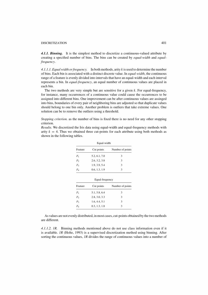
4.1.1. Binning. It is the simplest method to discretize a continuous-valued attribute bycreating a specified number of bins. The bins can be created by equal-width and equal-frequency.

4.1.1.1. Equal width or frequency. In both methods, arity k is used to determine the numberof bins. Each bin is associated with a distinct discrete value. In equal-width, the continuousrange of a feature is evenly divided into intervals that have an equal-width and each intervalrepresents a bin. In equal-frequency, an equal number of continuous values are placed ineach bin.

The two methods are very simple but are sensitive for a given k. For equal-frequency,for instance, many occurrences of a continuous value could cause the occurrences to beassigned into different bins. One improvement can be after continuous values are assingedinto bins, boundaries of every pair of neighboring bins are adjusted so that duplicate valuesshould belong to one bin only. Another problem is outliers that take extreme values. Onesolution can be to remove the outliers using a threshold.

Stopping criterion. as the number of bins is fixed there is no need for any other stoppingcriterion.Results. We discretized the Iris data using equal-width and equal-frequency methods witharity k = 4. Thus we obtained three cut-points for each attribute using both methods asshown in the following tables.

Equal-width

Feature Cut points Number of points

F1 5.2, 6.1, 7.0 3

F2 2.6, 3.2, 3.8 3

F3 1.9, 3.9, 5.4 3

F4 0.6, 1.3, 1.9 3

Equal-frequency

Feature Cut points Number of points

F1 5.1, 5.8, 6.4 3

F2 2.8, 3.0, 3.3 3

F3 1.6, 4.4, 5.1 3

F4 0.3, 1.3, 1.8 3

As values are not evenly distributed, in most cases, cut-points obtained by the two methodsare different.

4.1.1.2. 1R. Binning methods mentioned above do not use class information even if itis available. 1R (Holte, 1993) is a supervised discretization method using binning. Aftersorting the continuous values, 1R divides the range of continuous values into a number of

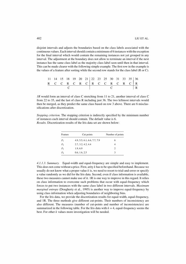
402 LIU ET AL.

disjoint intervals and adjusts the boundaries based on the class labels associated with thecontinuous values. Each interval should contain a minimum of 6 instances with the exceptionfor the final interval which would contain the remaining instances not yet grouped in anyinterval. The adjustment at the boundary does not allow to terminate an interval if the nextinstance has the same class label as the majority class label seen until then in that interval.This can be made clearer with the following simple example. The first row in the example isthe values of a feature after sorting while the second row stands for the class label (R or C).

11 14 15 18 19 20 21 22 23 25 30 31 33 35 36

R C C R C R C R C C R C R C RC C R

1R would form an interval of class C stretching from 11 to 21, another interval of class Cfrom 22 to 35, and the last of class R including just 36. The two leftmost intervals wouldthen be merged, as they predict the same class based on row 3 above. There are 6 misclas-sifications after discretization.

Stopping criterion. The stopping criterion is indirectly specified by the minimum numberof instances each interval should contain. The default value is 6.Results. Discretization results of the Iris data set are shown below:

Feature Cut points Number of points

F1 4.9, 5.5, 6.1, 6.6, 7.7, 7.9 6

F2 2.7, 3.2, 4.2, 4.4 4

F3 1.9, 6.9 2

F4 0.6, 1.6, 2.5 3

4.1.1.3. Summary. Equal-width and equal-frequency are simple and easy to implement.This does not come without a price. First, arity k has to be specified beforehand. Because weusually do not know what a proper value k is, we need to resort to trial-and-error or specifya value randomly as we did for the Iris data. Second, even if class information is available,these two measures cannot make use of it. 1R is one way to improve in this regard. It relieson class information to overcome such problems that occur with equal-frequency whichforces to put two instances with the same class label in two different intervals. Maximummarginal entropy (Dougherty et al., 1995) is another way to improve equal-frequency byusing class information when adjusting boundaries of neighboring bins.

For the Iris data, we provide the discretization results for equal-width, equal-frequency,and 1R. The three methods give different cut-points. Their numbers of inconsistency arealso different. The measures (number of cut-points and number of inconsistencies) aresummarized in the following table. For the Iris data with k = 4, equal-frequency seems thebest. For other k values more investigation will be needed.

DISCRETIZATION 403

Methods Inconsistency Number of points

Equal-width 10 12

Equal-freq 6 12

1R 7 15

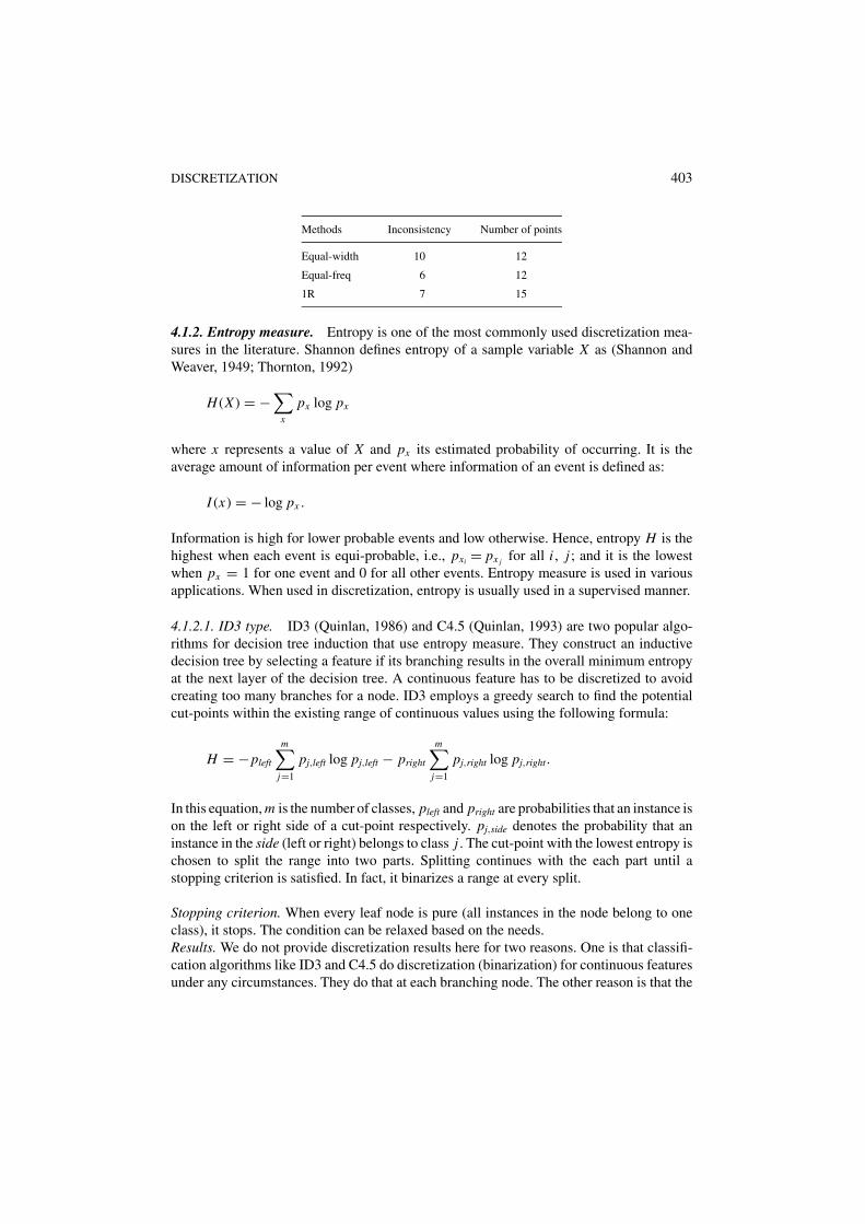
4.1.2. Entropy measure. Entropy is one of the most commonly used discretization mea-sures in the literature. Shannon defines entropy of a sample variable X as (Shannon andWeaver, 1949; Thornton, 1992)

H (X ) = −∑

x

px log px

where x represents a value of X and px its estimated probability of occurring. It is theaverage amount of information per event where information of an event is defined as:

I (x) = − log px .

Information is high for lower probable events and low otherwise. Hence, entropy H is thehighest when each event is equi-probable, i.e., pxi = px j for all i , j ; and it is the lowestwhen px = 1 for one event and 0 for all other events. Entropy measure is used in variousapplications. When used in discretization, entropy is usually used in a supervised manner.

4.1.2.1. ID3 type. ID3 (Quinlan, 1986) and C4.5 (Quinlan, 1993) are two popular algo-rithms for decision tree induction that use entropy measure. They construct an inductivedecision tree by selecting a feature if its branching results in the overall minimum entropyat the next layer of the decision tree. A continuous feature has to be discretized to avoidcreating too many branches for a node. ID3 employs a greedy search to find the potentialcut-points within the existing range of continuous values using the following formula:

H = −pleft

m∑

j=1

pj,left log pj,left − pright

m∑

j=1

pj,right log pj,right.

In this equation, m is the number of classes, pleft and pright are probabilities that an instance ison the left or right side of a cut-point respectively. pj,side denotes the probability that aninstance in the side (left or right) belongs to class j . The cut-point with the lowest entropy ischosen to split the range into two parts. Splitting continues with the each part until astopping criterion is satisfied. In fact, it binarizes a range at every split.

Stopping criterion. When every leaf node is pure (all instances in the node belong to oneclass), it stops. The condition can be relaxed based on the needs.Results. We do not provide discretization results here for two reasons. One is that classifi-cation algorithms like ID3 and C4.5 do discretization (binarization) for continuous featuresunder any circumstances. They do that at each branching node. The other reason is that the

404 LIU ET AL.

cut-points thus obtained are usually only good for the classification algorithm. We discussthis discretization method (binarization) here because it is a base for its many successorssuch as D2, MDLP.

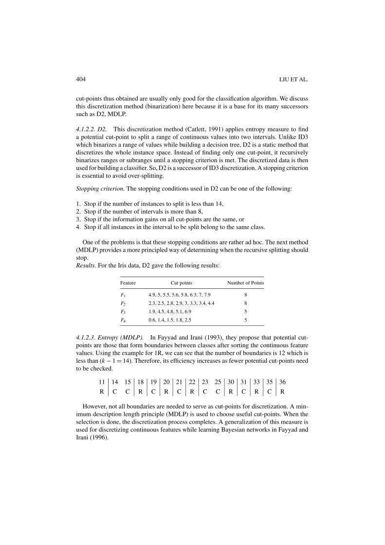
4.1.2.2. D2. This discretization method (Catlett, 1991) applies entropy measure to finda potential cut-point to split a range of continuous values into two intervals. Unlike ID3which binarizes a range of values while building a decision tree, D2 is a static method thatdiscretizes the whole instance space. Instead of finding only one cut-point, it recursivelybinarizes ranges or subranges until a stopping criterion is met. The discretized data is thenused for building a classifier. So, D2 is a successor of ID3 discretization. A stopping criterionis essential to avoid over-splitting.

Stopping criterion. The stopping conditions used in D2 can be one of the following:

1. Stop if the number of instances to split is less than 14,2. Stop if the number of intervals is more than 8,3. Stop if the information gains on all cut-points are the same, or4. Stop if all instances in the interval to be split belong to the same class.

One of the problems is that these stopping conditions are rather ad hoc. The next method(MDLP) provides a more principled way of determining when the recursive splitting shouldstop.Results. For the Iris data, D2 gave the following results:

Feature Cut points Number of Points

F1 4.9, 5, 5.5, 5.6, 5.8, 6.3, 7, 7.9 8

F2 2.3, 2.5, 2.8, 2.9, 3, 3.3, 3.4, 4.4 8

F3 1.9, 4.5, 4.8, 5.1, 6.9 5

F4 0.6, 1.4, 1.5, 1.8, 2.5 5

4.1.2.3. Entropy (MDLP). In Fayyad and Irani (1993), they propose that potential cut-points are those that form boundaries between classes after sorting the continuous featurevalues. Using the example for 1R, we can see that the number of boundaries is 12 which isless than (k − 1 = 14). Therefore, its efficiency increases as fewer potential cut-points needto be checked.

11 14 15 18 19 20 21 22 23 25 30 31 33 35 36

R C C R C R C R C C R C R C R

However, not all boundaries are needed to serve as cut-points for discretization. A min-imum description length principle (MDLP) is used to choose useful cut-points. When theselection is done, the discretization process completes. A generalization of this measure isused for discretizing continuous features while learning Bayesian networks in Fayyad andIrani (1996).

DISCRETIZATION 405

Stopping criterion. MDLP is used as stopping criterion. MDLP is usually formulated asa problem of finding the cost of communication between a sender and a receiver. It isassumed that the sender has the entire set of instances while the receiver has the class labelsof the instances. The sender needs to convey the proper class labeling of the instances to thereceiver. It says that the partition induced by a cut-point for a set of instances is accepted ifand only if the cost or length of the message required to send before partition is more thanthe cost or length of the message required to send after partition. A detailed account howthis is done can be found in Fayyad and Irani (1993).Results. Entropy (MDLP) discretized the Iris data as shown below.

Feature Cut points Number of points

F1 5.4, 6.1 2

F2 4.4 1

F3 1.9, 4.9, 6.9 3

F4 0.6, 1.6, 2.5 3

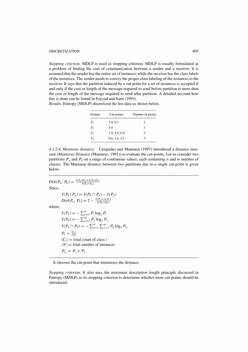
4.1.2.4. Mantaras distance. Cerquides and Mantaras (1997) introduced a distance mea-sure (Mantaras Distance (Mantaras, 1991)) to evaluate the cut-points. Let us consider twopartitions Pa and Pb on a range of continuous values, each containing n and m number ofclasses. The Mantaras distance between two partitions due to a single cut-point is givenbelow.

Dist(Pa, Pb) = I (Pa |Pb)+I (Pb|Pa )I (Pa∩Pb)

Since,

I (Pb | Pa) = I (Pb ∩ Pa) − I (Pa)

Dist(Pa, Pb) = 2 − I (Pa )+I (Pb)I (Pa∩Pb)

where,

I (Pa) = − ∑ni=1 Pi log2 Pi

I (Pb) = − ∑mj=1 Pj log2 Pj

I (Pa ∩ Pb) = − ∑ni=1

∑mj=1 Pij log2 Pi j

Pi = |Ci ||N |

|Ci | = total count of class i|N | = total number of instances

Pi j = Pi × Pj

It chooses the cut-point that minimizes the distance.

Stopping criterion. It also uses the minimum description length principle discussed inEntropy (MDLP) as its stopping criterion to determine whether more cut-points should beintroduced.

406 LIU ET AL.

Results. Using this distance, we obtained results for the Iris data below.

Feature Cut points Number of points

F1 5.7, 7.9 2

F2 3, 4.4 2

F3 1.9, 4.4, 5.1, 6.9 4

F4 0.6, 1.3, 1.8, 2.5 4

4.1.2.5. Summary. ID3 type applies binarization to discretize continuous values whilebuilding a tree. D2 does better by separating discretization from tree building and by recur-sively binarizing ranges and/or subranges. Its problem is that there is no principled way tostop its recursive process of binarization. Entropy (MDLP) uses the minimum descriptionlength principle to determine when to stop discretization. It also suggests that potential cut-points are those that separate different class values. Based on the summary of results in thefollowing table for the Iris data, MDLP is an obvious winner as it produces comparativelylow inconsistencies and cut-points.

Methods Inconsistency Number of points

D2 1 26

MDLP 3 9

Mantaras 8 12

Another work using entropy can be found in Van de Merckt (1990). A contrast measureis introduced that uses the clustering concept to get the cut-point to induce a decision tree.The idea is to search for clusters that are contrasted as much as possible from the instancespace proximity point of view. The cut-point for the maximum contrast is chosen. But thecut-point selected must be an informative one, i.e., it is uninformative to select a cut-pointthat separates instances belonging to the same class. So, an entropy measure is proposed toselect cut-points further. As it is mainly suggested in the context of tree building, we stopshort of discussing it here and refer the interesting reader to Van de Merckt (1990) for moredetails.

4.1.3. Dependency

4.1.3.1. Zeta. It is a measure of strength of association between the class and a feature. InHo and Scott (1997), it is defined as the maximum accuracy achievable when each valueof a feature predicts a different class value. We use a simple case to illustrate how Zeta iscalculated. Assume that there is a continuous feature X with two classes (C1 and C2). Thetask is to find one cut-point (two intervals) at a time with the highest Z (zeta) value.

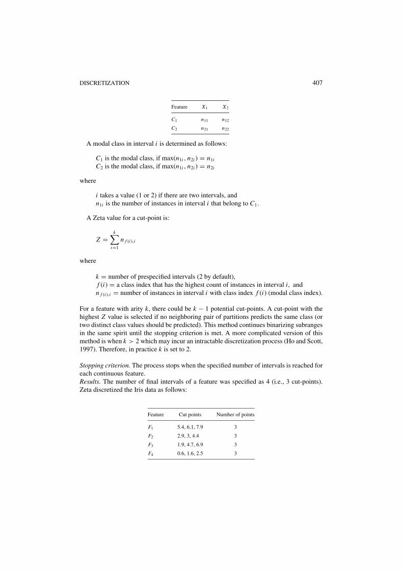
DISCRETIZATION 407

Feature X1 X2

C1 n11 n12

C2 n21 n22

A modal class in interval i is determined as follows:

C1 is the modal class, if max(n1i , n2i ) = n1i

C2 is the modal class, if max(n1i , n2i ) = n2i

where

i takes a value (1 or 2) if there are two intervals, andn1i is the number of instances in interval i that belong to C1.

A Zeta value for a cut-point is:

Z =k∑

i=1

n f (i),i

where

k = number of prespecified intervals (2 by default),f (i) = a class index that has the highest count of instances in interval i, andn f (i),i = number of instances in interval i with class index f (i) (modal class index).

For a feature with arity k, there could be k − 1 potential cut-points. A cut-point with thehighest Z value is selected if no neighboring pair of partitions predicts the same class (ortwo distinct class values should be predicted). This method continues binarizing subrangesin the same spirit until the stopping criterion is met. A more complicated version of thismethod is when k > 2 which may incur an intractable discretization process (Ho and Scott,1997). Therefore, in practice k is set to 2.

Stopping criterion. The process stops when the specified number of intervals is reached foreach continuous feature.Results. The number of final intervals of a feature was specified as 4 (i.e., 3 cut-points).Zeta discretized the Iris data as follows:

Feature Cut points Number of points

F1 5.4, 6.1, 7.9 3

F2 2.9, 3, 4.4 3

F3 1.9, 4.7, 6.9 3

F4 0.6, 1.6, 2.5 3

408 LIU ET AL.

Method Inconsistency Number of points

Zeta 3 12

Zeta obtained reasonable discretization results for this data. Clearly, with a differentnumber of final intervals, the results will certainly change. We could also allow differentfeatures to have different final intervals if we have some prior knowledge about them.

4.1.4. Accuracy. Accuracy measure usually means the accuracy of a classifier. An exampleof using accuracy for discretization is Adaptive Quantizer (Chan et al., 1991). It considershow well one attribute predicts the class at a time. For each attribute, its continuous range issplit into two partitions either by equal-frequency or by equal-width. The splitting is testedby running a classifier to see if the splitting helps improve accuracy. It continues binarizingsubranges and the cut-point which gives the minimum rate is selected. As it involves traininga classifier, it is usually more time consuming than those without using a classifier.

Stopping criterion. For each attribute, the discretization process stops when there is noimprovement in accuracy.Results. We used C4.5 as the classifier to see the improvement while splitting the attributevalues using equal-width.

Feature Cut points Number of points

F1 5.20, 6.10 2

F2 2.60, 3.20 2

F3 2.47, 3.95, 5.42 3

F4 0.70, 1.30, 1.90 3

Method Inconsistency Number of points

Accuracy 10 10

The choice of a classifier depends on a user’s preferences. However, as the classifierneed to be trained many times, it is necessary to choose one with small time complexity.For example, C4.5 runs reasonably fast with time complexity O(N log N ) where N is thenumber of instances.

4.2. Merging methods

We start with a generalized algorithm for discretization methods adopting the merging orbottom-up approach.

DISCRETIZATION 409

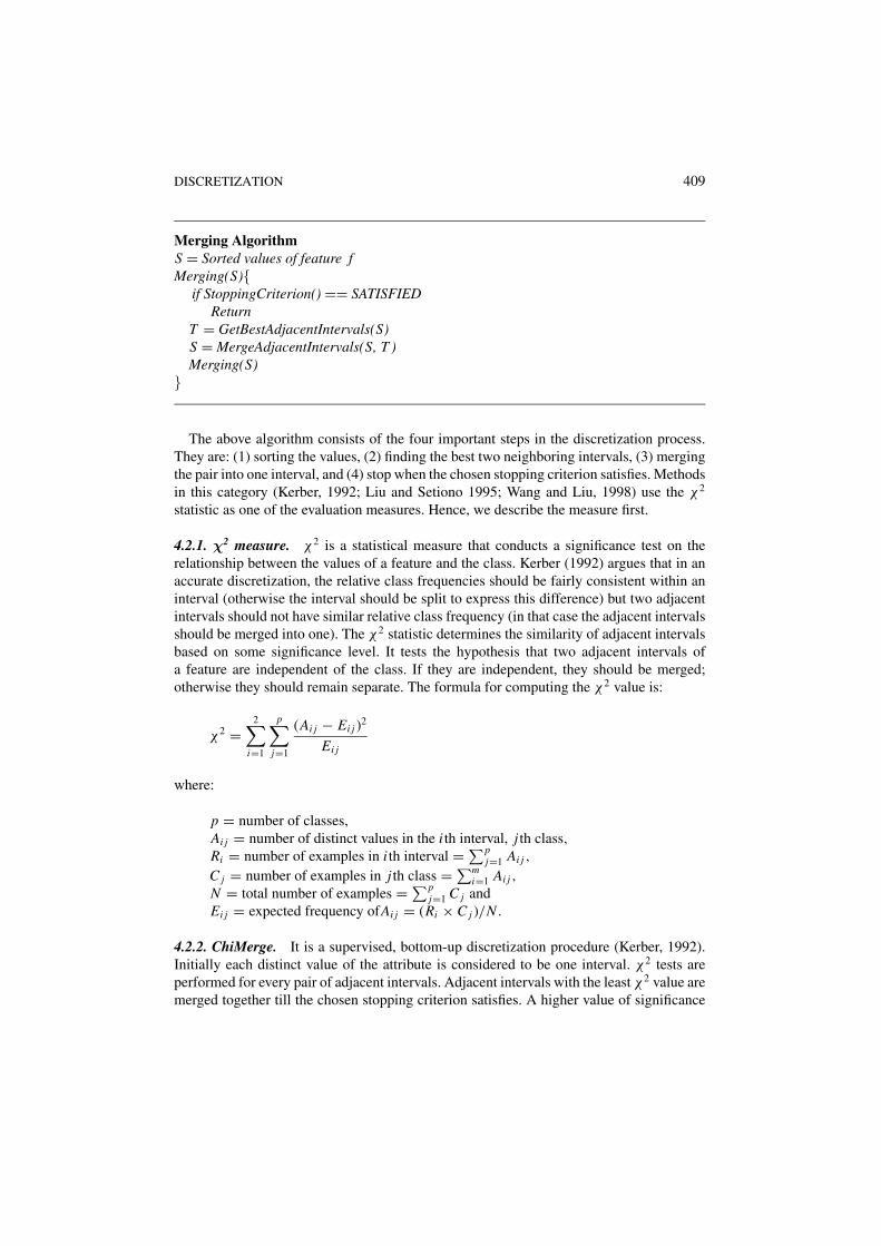
Merging AlgorithmS = Sorted values of feature fMerging(S){

if StoppingCriterion() == SATISFIEDReturn

T = GetBestAdjacentIntervals(S)S = MergeAdjacentIntervals(S, T )Merging(S)

}

The above algorithm consists of the four important steps in the discretization process.They are: (1) sorting the values, (2) finding the best two neighboring intervals, (3) mergingthe pair into one interval, and (4) stop when the chosen stopping criterion satisfies. Methodsin this category (Kerber, 1992; Liu and Setiono 1995; Wang and Liu, 1998) use the χ2

statistic as one of the evaluation measures. Hence, we describe the measure first.

4.2.1. χ2 measure. χ2 is a statistical measure that conducts a significance test on therelationship between the values of a feature and the class. Kerber (1992) argues that in anaccurate discretization, the relative class frequencies should be fairly consistent within aninterval (otherwise the interval should be split to express this difference) but two adjacentintervals should not have similar relative class frequency (in that case the adjacent intervalsshould be merged into one). The χ2 statistic determines the similarity of adjacent intervalsbased on some significance level. It tests the hypothesis that two adjacent intervals ofa feature are independent of the class. If they are independent, they should be merged;otherwise they should remain separate. The formula for computing the χ2 value is:

χ2 =2∑

i=1

p∑

j=1

(Ai j − Ei j )2

Ei j

where:

p = number of classes,Ai j = number of distinct values in the i th interval, j th class,Ri = number of examples in i th interval = ∑p

j=1 Ai j ,

C j = number of examples in j th class = ∑mi=1 Ai j ,

N = total number of examples = ∑pj=1 C j and

Ei j = expected frequency ofAi j = (Ri × C j )/N .

4.2.2. ChiMerge. It is a supervised, bottom-up discretization procedure (Kerber, 1992).Initially each distinct value of the attribute is considered to be one interval. χ2 tests areperformed for every pair of adjacent intervals. Adjacent intervals with the least χ2 value aremerged together till the chosen stopping criterion satisfies. A higher value of significance

410 LIU ET AL.

level for χ2 test causes over discretization while a lower value causes under discretization.The recommended procedure is to set the significance level between 0.90 to 0.99 and havea max-interval parameter set to 10 or 15. This max-interval parameter can be included toavoid the excessive number of intervals from being created.

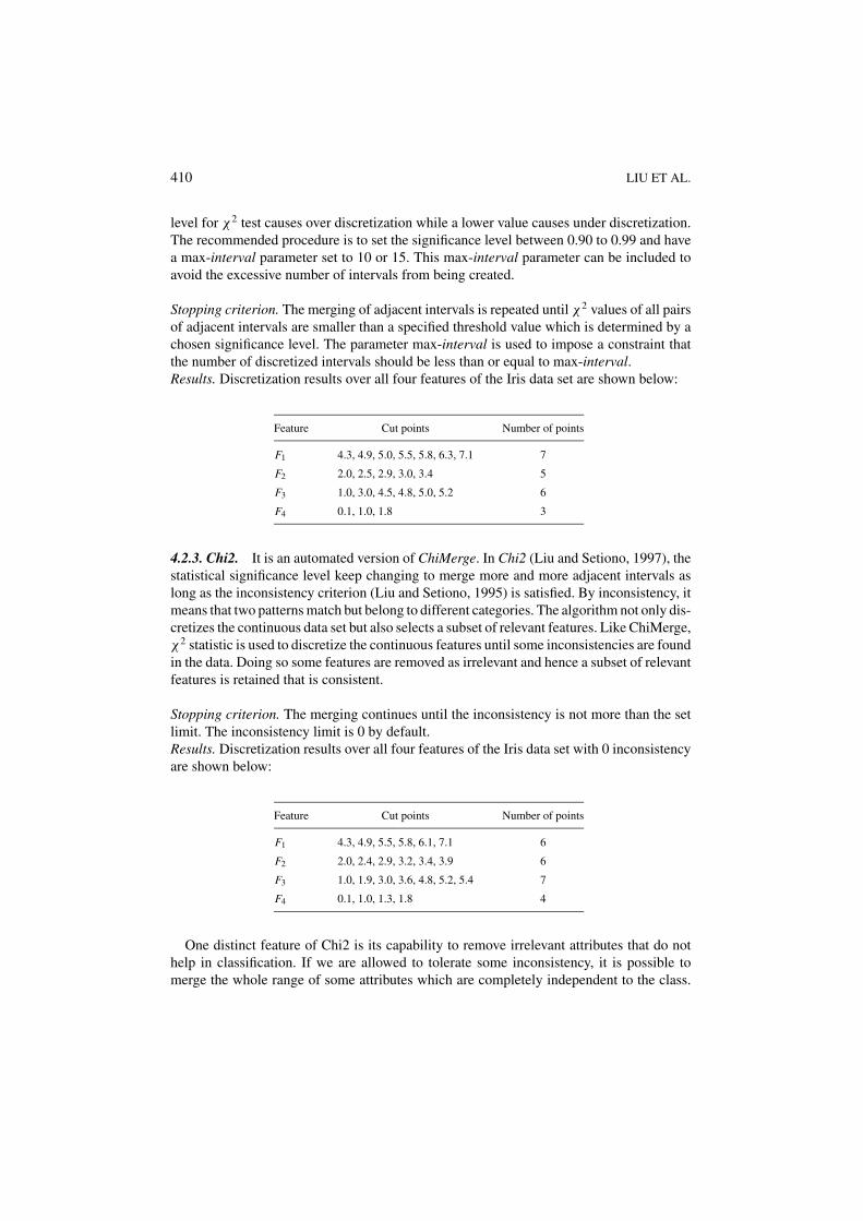
Stopping criterion. The merging of adjacent intervals is repeated until χ2 values of all pairsof adjacent intervals are smaller than a specified threshold value which is determined by achosen significance level. The parameter max-interval is used to impose a constraint thatthe number of discretized intervals should be less than or equal to max-interval.Results. Discretization results over all four features of the Iris data set are shown below:

Feature Cut points Number of points

F1 4.3, 4.9, 5.0, 5.5, 5.8, 6.3, 7.1 7

F2 2.0, 2.5, 2.9, 3.0, 3.4 5

F3 1.0, 3.0, 4.5, 4.8, 5.0, 5.2 6

F4 0.1, 1.0, 1.8 3

4.2.3. Chi2. It is an automated version of ChiMerge. In Chi2 (Liu and Setiono, 1997), thestatistical significance level keep changing to merge more and more adjacent intervals aslong as the inconsistency criterion (Liu and Setiono, 1995) is satisfied. By inconsistency, itmeans that two patterns match but belong to different categories. The algorithm not only dis-cretizes the continuous data set but also selects a subset of relevant features. Like ChiMerge,χ2 statistic is used to discretize the continuous features until some inconsistencies are foundin the data. Doing so some features are removed as irrelevant and hence a subset of relevantfeatures is retained that is consistent.

Stopping criterion. The merging continues until the inconsistency is not more than the setlimit. The inconsistency limit is 0 by default.Results. Discretization results over all four features of the Iris data set with 0 inconsistencyare shown below:

Feature Cut points Number of points

F1 4.3, 4.9, 5.5, 5.8, 6.1, 7.1 6

F2 2.0, 2.4, 2.9, 3.2, 3.4, 3.9 6

F3 1.0, 1.9, 3.0, 3.6, 4.8, 5.2, 5.4 7

F4 0.1, 1.0, 1.3, 1.8 4

One distinct feature of Chi2 is its capability to remove irrelevant attributes that do nothelp in classification. If we are allowed to tolerate some inconsistency, it is possible tomerge the whole range of some attributes which are completely independent to the class.

DISCRETIZATION 411

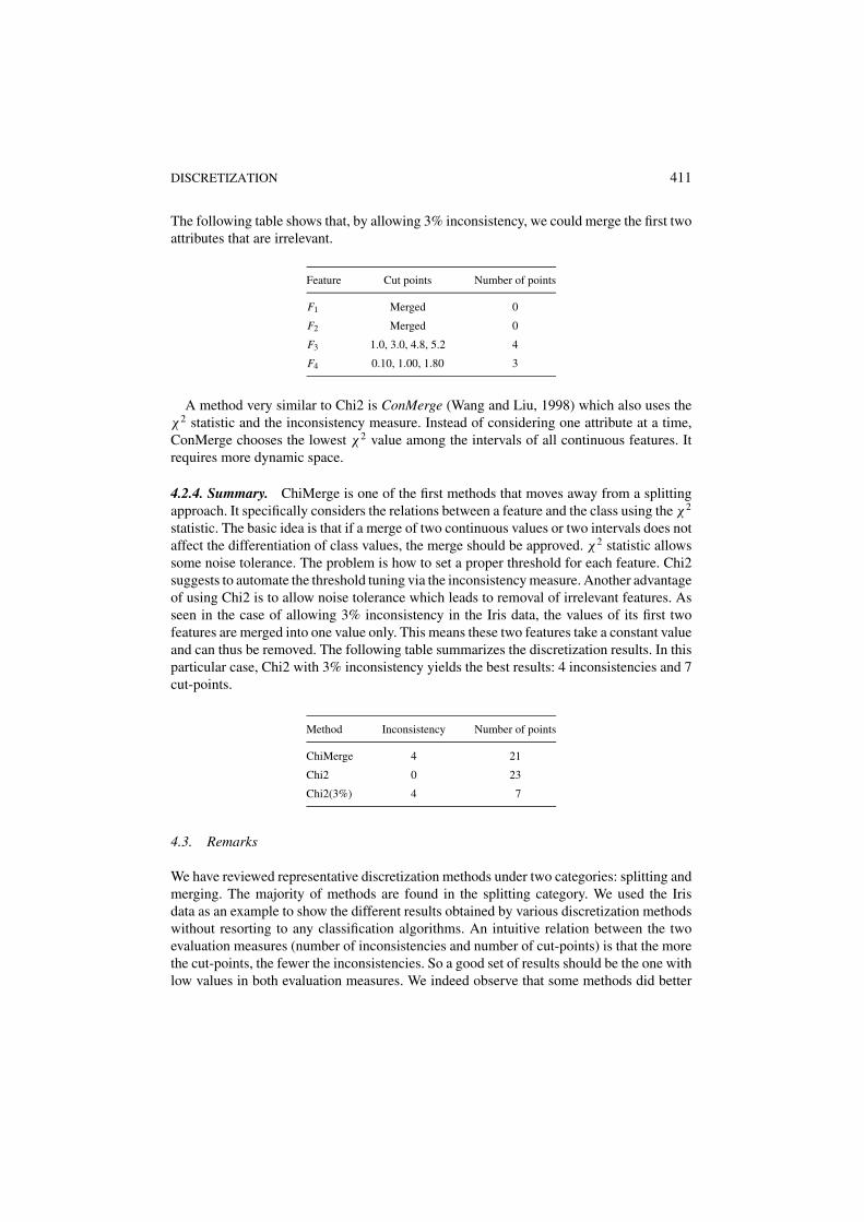
The following table shows that, by allowing 3% inconsistency, we could merge the first twoattributes that are irrelevant.

Feature Cut points Number of points

F1 Merged 0

F2 Merged 0

F3 1.0, 3.0, 4.8, 5.2 4

F4 0.10, 1.00, 1.80 3

A method very similar to Chi2 is ConMerge (Wang and Liu, 1998) which also uses theχ2 statistic and the inconsistency measure. Instead of considering one attribute at a time,ConMerge chooses the lowest χ2 value among the intervals of all continuous features. Itrequires more dynamic space.

4.2.4. Summary. ChiMerge is one of the first methods that moves away from a splittingapproach. It specifically considers the relations between a feature and the class using the χ2

statistic. The basic idea is that if a merge of two continuous values or two intervals does notaffect the differentiation of class values, the merge should be approved. χ2 statistic allowssome noise tolerance. The problem is how to set a proper threshold for each feature. Chi2suggests to automate the threshold tuning via the inconsistency measure. Another advantageof using Chi2 is to allow noise tolerance which leads to removal of irrelevant features. Asseen in the case of allowing 3% inconsistency in the Iris data, the values of its first twofeatures are merged into one value only. This means these two features take a constant valueand can thus be removed. The following table summarizes the discretization results. In thisparticular case, Chi2 with 3% inconsistency yields the best results: 4 inconsistencies and 7cut-points.

Method Inconsistency Number of points

ChiMerge 4 21

Chi2 0 23

Chi2(3%) 4 7

4.3. Remarks

We have reviewed representative discretization methods under two categories: splitting andmerging. The majority of methods are found in the splitting category. We used the Irisdata as an example to show the different results obtained by various discretization methodswithout resorting to any classification algorithms. An intuitive relation between the twoevaluation measures (number of inconsistencies and number of cut-points) is that the morethe cut-points, the fewer the inconsistencies. So a good set of results should be the one withlow values in both evaluation measures. We indeed observe that some methods did better

412 LIU ET AL.

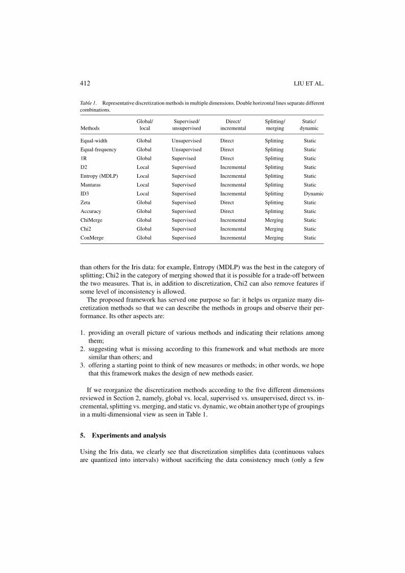
Table 1. Representative discretization methods in multiple dimensions. Double horizontal lines separate differentcombinations.

Global/ Supervised/ Direct/ Splitting/ Static/Methods local unsupervised incremental merging dynamic

Equal-width Global Unsupervised Direct Splitting Static

Equal-frequency Global Unsupervised Direct Splitting Static

1R Global Supervised Direct Splitting Static

D2 Local Supervised Incremental Splitting Static

Entropy (MDLP) Local Supervised Incremental Splitting Static

Mantaras Local Supervised Incremental Splitting Static

ID3 Local Supervised Incremental Splitting Dynamic

Zeta Global Supervised Direct Splitting Static

Accuracy Global Supervised Direct Splitting Static

ChiMerge Global Supervised Incremental Merging Static

Chi2 Global Supervised Incremental Merging Static

ConMerge Global Supervised Incremental Merging Static

than others for the Iris data: for example, Entropy (MDLP) was the best in the category ofsplitting; Chi2 in the category of merging showed that it is possible for a trade-off betweenthe two measures. That is, in addition to discretization, Chi2 can also remove features ifsome level of inconsistency is allowed.

The proposed framework has served one purpose so far: it helps us organize many dis-cretization methods so that we can describe the methods in groups and observe their per-formance. Its other aspects are:

1. providing an overall picture of various methods and indicating their relations amongthem;

2. suggesting what is missing according to this framework and what methods are moresimilar than others; and

3. offering a starting point to think of new measures or methods; in other words, we hopethat this framework makes the design of new methods easier.

If we reorganize the discretization methods according to the five different dimensionsreviewed in Section 2, namely, global vs. local, supervised vs. unsupervised, direct vs. in-cremental, splitting vs. merging, and static vs. dynamic, we obtain another type of groupingsin a multi-dimensional view as seen in Table 1.

5. Experiments and analysis

Using the Iris data, we clearly see that discretization simplifies data (continuous valuesare quantized into intervals) without sacrificing the data consistency much (only a few

DISCRETIZATION 413

inconsistencies occur after discretization). We are now ready to evaluate the ultimate objec-tive of discretization—whether discretization helps improve the performance of learningand understanding of the learning result. The improvement can be measured in three aspectsthrough before/after discretization comparison: (1) accuracy, (2) time for discretization andfor learning, and (3) understandability of the learning result. Thus, we need a classificationlearning algorithm. A critical constraint for choosing such a learning algorithm is that itshould be able to run with both data types, i.e., continuous as well as discrete. Not ev-ery learning algorithm can do so. Naive Bayes Classifier (Domingos and Pazzani, 1996;Kontkaren, et al., 1998), as an example, can only run on discrete data. C4.5 (Quinlan, 1993)is chosen for experiments because it can handle both data types and it is conveniently avail-able and widely used so that a reader can easily repeat the experiments here. Furthermore,C4.5 has become a de facto standard for comparison in machine learning. We have reimple-mented the discretization methods used in the experiments based on the descriptions of thepublished papers. The programs of these discretization algorithms are available throughftp or web access free of charge upon request. We will examine the effect of discretizationon C4.5 through comparisons before/after discretization. Before doing so, we outline thespecific meaning of each aspect of evaluation.

• Accuracy—we wish to see if discretization would result in the decrease or increase ofaccuracy. The usual 10-fold cross validation procedure will be used.

• Time for discretization—we wish to see if a discretization method that takes more timewould result in better accuracy.

• Time for learning with different data types of the same data—with which data types thelearning requires more time to complete.

• Understandability—the learning result of C4.5 is a decision tree. This aspect is indirectlymeasured through the number of nodes in a tree.

5.1. Experiment set-up

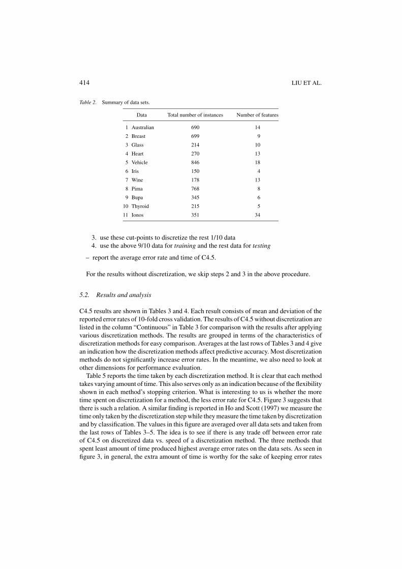
Eleven data sets are selected from the UC Irvine machine learning data repository (Merzand Murphy, 1996) with all numeric features and varying data sizes. A summary of data setscan be found in Table 2. A total of 8 discretization methods excluding ID3 type are chosento compare according to Table 1 excluding Equal-width, and Accuracy. Accuracy methodtakes too long time as every selection of a cut-point evokes a decision tree learning. ID3 typeis used as the base for comparison, as we use C4.5 (an improved version of ID3) to providethe figures of performance before discretization. Equal-width is similar to Equal-Freq. Wechoose the latter based on our experience gained in Section 4.

Each experiment is conducted as follows:

• for each data set

– test each discretization method by 10-fold cross validation of C4.5

1. take every 9/10 of the data in each round (10 in total)2. run a discretization method to get cut-points, measure the time needed

414 LIU ET AL.

Table 2. Summary of data sets.

Data Total number of instances Number of features

1 Australian 690 14

2 Breast 699 9

3 Glass 214 10

4 Heart 270 13

5 Vehicle 846 18

6 Iris 150 4

7 Wine 178 13

8 Pima 768 8

9 Bupa 345 6

10 Thyroid 215 5

11 Ionos 351 34

3. use these cut-points to discretize the rest 1/10 data4. use the above 9/10 data for training and the rest data for testing

– report the average error rate and time of C4.5.

For the results without discretization, we skip steps 2 and 3 in the above procedure.

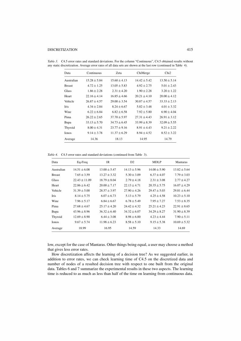
5.2. Results and analysis

C4.5 results are shown in Tables 3 and 4. Each result consists of mean and deviation of thereported error rates of 10-fold cross validation. The results of C4.5 without discretization arelisted in the column “Continuous” in Table 3 for comparison with the results after applyingvarious discretization methods. The results are grouped in terms of the characteristics ofdiscretization methods for easy comparison. Averages at the last rows of Tables 3 and 4 givean indication how the discretization methods affect predictive accuracy. Most discretizationmethods do not significantly increase error rates. In the meantime, we also need to look atother dimensions for performance evaluation.

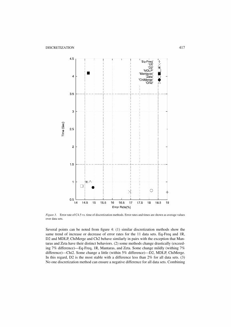
Table 5 reports the time taken by each discretization method. It is clear that each methodtakes varying amount of time. This also serves only as an indication because of the flexibilityshown in each method’s stopping criterion. What is interesting to us is whether the moretime spent on discretization for a method, the less error rate for C4.5. Figure 3 suggests thatthere is such a relation. A similar finding is reported in Ho and Scott (1997) we measure thetime only taken by the discretization step while they measure the time taken by discretizationand by classification. The values in this figure are averaged over all data sets and taken fromthe last rows of Tables 3–5. The idea is to see if there is any trade off between error rateof C4.5 on discretized data vs. speed of a discretization method. The three methods thatspent least amount of time produced highest average error rates on the data sets. As seen infigure 3, in general, the extra amount of time is worthy for the sake of keeping error rates

DISCRETIZATION 415

Table 3. C4.5 error rates and standard deviations. For the column “Continuous”, C4.5 obtained results withoutany static discretization. Average error rates of all data sets are shown at the last row (continued in Table 4).

Data Continuous Zeta ChiMerge Chi2

Australian 15.28 ± 5.84 15.60 ± 4.13 14.42 ± 5.42 13.50 ± 5.14

Breast 4.72 ± 1.25 13.05 ± 5.83 4.92 ± 2.75 5.01 ± 2.43

Glass 1.86 ± 2.28 2.31 ± 4.20 1.90 ± 2.28 3.20 ± 1.22

Heart 22.16 ± 4.14 16.85 ± 4.66 20.21 ± 4.10 20.00 ± 4.12

Vehicle 26.87 ± 4.57 29.00 ± 3.54 30.87 ± 4.57 33.33 ± 2.13

Iris 4.34 ± 2.84 8.24 ± 6.67 5.02 ± 3.48 4.01 ± 3.32

Wine 6.22 ± 6.84 6.82 ± 6.58 7.92 ± 5.80 6.90 ± 4.04

Pima 26.22 ± 2.65 37.70 ± 5.97 27.31 ± 4.43 26.91 ± 3.12

Bupa 33.13 ± 5.70 34.73 ± 6.45 33.99 ± 8.39 32.09 ± 5.55

Thyroid 8.00 ± 4.31 23.77 ± 9.16 8.91 ± 4.43 9.21 ± 2.22

Ionos 9.14 ± 3.78 11.37 ± 6.29 8.94 ± 4.52 8.52 ± 3.22

Average 14.36 18.13 14.95 14.79

Table 4. C4.5 error rates and standard deviations (continued from Table 3).

Data Eq-Freq 1R D2 MDLP Mantaras

Australian 14.51 ± 6.08 13.00 ± 5.47 14.13 ± 5.96 14.00 ± 5.90 13.82 ± 5.64

Breast 7.65 ± 3.59 13.27 ± 3.32 5.30 ± 3.09 6.37 ± 4.07 7.79 ± 3.03

Glass 22.43 ± 11.09 18.79 ± 8.04 2.79 ± 4.18 2.31 ± 3.08 2.77 ± 4.27

Heart 22.86 ± 6.42 20.00 ± 7.17 22.13 ± 4.71 20.35 ± 5.75 16.07 ± 4.29

Vehicle 31.39 ± 5.00 28.57 ± 3.97 27.90 ± 4.26 29.47 ± 5.03 29.81 ± 6.44

Iris 8.14 ± 5.75 6.07 ± 6.73 5.13 ± 5.79 4.25 ± 4.58 10.23 ± 5.10

Wine 7.96 ± 5.17 6.84 ± 6.67 6.78 ± 5.49 7.95 ± 7.27 7.53 ± 8.35

Pima 27.68 ± 4.67 25.17 ± 4.20 24.42 ± 4.32 25.21 ± 4.23 22.91 ± 8.65

Bupa 43.96 ± 8.96 36.32 ± 6.40 34.32 ± 6.07 34.29 ± 8.27 31.90 ± 8.39

Thyroid 12.69 ± 8.90 6.44 ± 3.08 8.98 ± 6.00 4.23 ± 4.44 7.90 ± 5.11

Ionos 9.67 ± 5.74 11.98 ± 6.23 8.58 ± 5.10 9.15 ± 5.38 10.69 ± 5.32

Average 18.99 16.95 14.59 14.33 14.69

low, except for the case of Mantaras. Other things being equal, a user may choose a methodthat gives less error rates.

How discretization affects the learning of a decision tree? As we suggested earlier, inaddition to error rates, we can check learning time of C4.5 on the discretized data andnumber of nodes of a resulted decision tree with respect to one built from the originaldata. Tables 6 and 7 summarize the experimental results in these two aspects. The learningtime is reduced to as much as less than half of the time on learning from continuous data.

416 LIU ET AL.

Table 5. Time taken for discretization.

Data Eq-Freq 1R D2 MDLP Mantaras Zeta ChiMerge Chi2

Australian 0.87 0.68 1.43 1.51 5.97 0.72 1.16 2.01

Breast 0.79 0.78 0.92 0.74 1.85 0.77 0.72 0.92

Glass 0.29 0.28 0.45 0.71 1.40 0.36 0.37 0.41

Heart 0.33 0.37 0.51 0.45 0.93 0.34 0.46 0.55

Vehicle 1.85 1.88 2.74 1.90 16.55 2.04 2.08 2.10

Iris 0.71 0.76 1.00 0.65 2.25 0.80 0.96 1.02

Wine 0.29 0.30 0.42 0.45 1.76 0.33 0.43 0.55

Pima 0.70 0.75 0.92 0.91 5.62 0.73 0.55 0.61

Bupa 0.24 0.26 0.33 0.33 0.46 0.28 0.29 0.31

Thyroid 0.13 0.15 0.21 0.22 0.80 0.18 0.19 0.21

Ionos 1.62 1.75 2.10 1.87 7.41 1.79 2.08 2.32

Average 0.71 0.72 1.00 0.89 4.09 0.76 0.84 1.00

Table 6. Time required to learn by C4.5 before and after discretization.

Data Continuous Eq-Freq 1R D2 MDLP Mantaras Zeta ChiMerge Chi2

Australian 0.43 0.31 0.27 0.27 0.31 0.26 0.22 0.28 0.10

Breast 0.13 0.06 0.09 0.15 0.10 0.10 0.14 0.13 0.15

Glass 0.10 0.03 0.07 0.04 0.06 0.06 0.06 0.10 0.05

Heart 0.19 0.04 0.08 0.12 0.11 0.09 0.08 0.12 0.04

Vehicle 0.89 0.46 0.57 0.53 0.85 0.54 0.57 0.71 0.82

Iris 0.01 0.02 0.02 0.01 0.01 0.03 0.02 0.01 0.01

Wine 0.12 0.06 0.07 0.05 0.06 0.04 0.04 0.09 0.02

Pima 0.31 0.23 0.21 0.20 0.20 0.30 0.10 0.16 0.11

Bupa 0.11 0.12 0.12 0.07 0.15 0.11 0.04 0.11 0.09

Thyroid 0.05 0.04 0.02 0.06 0.04 0.02 0.02 0.09 0.02

Ionos 1.12 0.75 0.34 0.24 0.34 0.75 0.22 0.20 0.24

Average 0.31 0.19 0.16 0.15 0.20 0.20 0.13 0.18 0.15

All discretization methods contribute to time saving in learning. This is consistent withsome theoretical findings in Utogoff (1989) and Oates and Jensen (1999) that numeric datatypically requires repetitive sorting, so it needs a log N factor at each node for C4.5; butnot so for discrete data. The average number of nodes in a decision tree for all the data setsis also reduced.

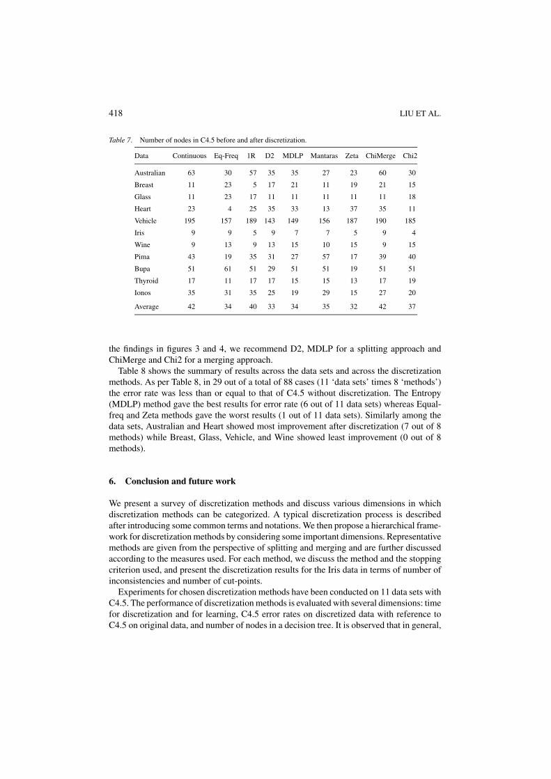
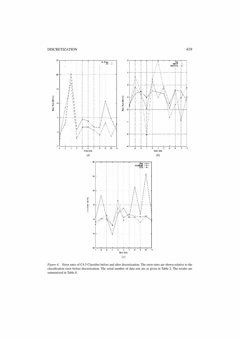
In order to facilitate our understanding of different discretization methods in their groups,we show the eight discretization methods in figure 4(a)–(c) using the result of C4.5 withoutdiscretization as the reference. A negative difference means an improvement in accuracy.

DISCRETIZATION 417

Figure 3. Error rate of C4.5 vs. time of discretization methods. Error rates and times are shown as average valuesover data sets.

Several points can be noted from figure 4: (1) similar discretization methods show thesame trend of increase or decrease of error rates for the 11 data sets. Eq-Freq and 1R,D2 and MDLP, ChiMerge and Ch2 behave similarly in pairs with the exception that Man-taras and Zeta have their distinct behaviors. (2) some methods change drastically (exceed-ing 7% difference)—Eq-Freq, 1R, Mantaras, and Zeta. Some change mildly (withing 7%difference)—Chi2. Some change a little (within 5% difference)—D2, MDLP, ChiMerge.In this regard, D2 is the most stable with a difference less than 2% for all data sets. (3)No one discretization method can ensure a negative difference for all data sets. Combining

418 LIU ET AL.

Table 7. Number of nodes in C4.5 before and after discretization.

Data Continuous Eq-Freq 1R D2 MDLP Mantaras Zeta ChiMerge Chi2

Australian 63 30 57 35 35 27 23 60 30

Breast 11 23 5 17 21 11 19 21 15

Glass 11 23 17 11 11 11 11 11 18

Heart 23 4 25 35 33 13 37 35 11

Vehicle 195 157 189 143 149 156 187 190 185

Iris 9 9 5 9 7 7 5 9 4

Wine 9 13 9 13 15 10 15 9 15

Pima 43 19 35 31 27 57 17 39 40

Bupa 51 61 51 29 51 51 19 51 51

Thyroid 17 11 17 17 15 15 13 17 19

Ionos 35 31 35 25 19 29 15 27 20

Average 42 34 40 33 34 35 32 42 37

the findings in figures 3 and 4, we recommend D2, MDLP for a splitting approach andChiMerge and Chi2 for a merging approach.

Table 8 shows the summary of results across the data sets and across the discretizationmethods. As per Table 8, in 29 out of a total of 88 cases (11 ‘data sets’ times 8 ‘methods’)the error rate was less than or equal to that of C4.5 without discretization. The Entropy(MDLP) method gave the best results for error rate (6 out of 11 data sets) whereas Equal-freq and Zeta methods gave the worst results (1 out of 11 data sets). Similarly among thedata sets, Australian and Heart showed most improvement after discretization (7 out of 8methods) while Breast, Glass, Vehicle, and Wine showed least improvement (0 out of 8methods).

6. Conclusion and future work

We present a survey of discretization methods and discuss various dimensions in whichdiscretization methods can be categorized. A typical discretization process is describedafter introducing some common terms and notations. We then propose a hierarchical frame-work for discretization methods by considering some important dimensions. Representativemethods are given from the perspective of splitting and merging and are further discussedaccording to the measures used. For each method, we discuss the method and the stoppingcriterion used, and present the discretization results for the Iris data in terms of number ofinconsistencies and number of cut-points.

Experiments for chosen discretization methods have been conducted on 11 data sets withC4.5. The performance of discretization methods is evaluated with several dimensions: timefor discretization and for learning, C4.5 error rates on discretized data with reference toC4.5 on original data, and number of nodes in a decision tree. It is observed that in general,

DISCRETIZATION 419

Figure 4. Error rates of C4.5 Classifier before and after discretization. The error rates are shown relative to theclassification error before discretization. The serial number of data sets are as given in Table 2. The results aresummarized in Table 8.

420 LIU ET AL.

Table 8. Summary of results for C4.5: Column (a) shows the number of methods for each data set for whichC4.5 performs better than without discretization. Column (b) shows the number of data sets for each method forwhich C4.5 performs better than without discretization.

a b

Data set Number of MethodBetter Method Number of DataBetter

1. Australian 7/8 Eq-Freq 1/11

2. Breast 0/8 1R 4/11

3. Glass 0/8 D2 4/11

4. Heart 7/8 MDLP 6/11

5. Vehicle 0/8 Mantaras 5/11

6. Iris 2/8 Zeta 1/11

7. Wine 0/8 ChiMerge 3/11

8. Pima 4/8 Chi2 5/11

9. Bupa 2/8

10. Thyroid 3/8

11. Ionos 4/8

more time on discretization leads to better accuracy for C4.5. Our findings in Sections 4 and5 are pretty consistent as both point toward Entropy (MDLP) being identified as the firstchoice. However, choosing a suitable discretization method is generally a complex matter,and largely depends on a user’s need and other considerations of discretization, as well ason what kind of data to be discretized. If the data does not have class information, onlyunsupervised methods can be applied. When class information is available, a supervisedmethod should be employed. Do we wish to remove redundant/irrelevant features? If so,Chi2 is a choice. If we need to incorporate discretization into a learning process, dynamicdiscretization methods such as ID3, Contrast should be considered. To reiterate, if we simplywant to discretize data, other things being equal, Entropy (MDLP) should be the first choiceto consider.

A reader may notice that every discretization method discussed takes it for granted thateach feature independently determines the class. Therefore, all these methods are univariatemethods for the sake of efficiency. As we know, the assumption may not be valid. Whenwe discretize, we may need to consider multiple features at a time, the so-called multivari-ate discretization. Doing so would inevitably increase time complexity for discretization.Using the inconsistency measure in Chi2 is one effort towards taking into account the jointcontribution of features. With the availability of more powerful parallel computers or com-puter clusters, we may investigate the possibility of using these computers for multivariatediscretization. Parallel discretization algorithms are surely welcome when a large numberof continuous features should be quantized. Can we extend the methods here to parallelizedversions? With the feature independence assumption, it seems practical. Sometimes, a dataset consists of various types of features. In Chi2, concepts of over/under discretization aresuggested to account for mixed types of features (Liu and Setiono, 1997). Again, mixedtypes of features would not cause a problem if the feature independence assumption is

DISCRETIZATION 421

acceptable. It is obviously not the case in the context of multivariate discretization. Noisehandling is another important issue of discretization in practice. To allow a certain degree oftolerance via thresholding is a common practice for noise handling in the methods discussedhere. Chi2 suggests to use the number of inconsistencies as a way to handle one type ofnoise. However, it seems an impasse when no prior knowledge about noise is available. Allin all, this paper is not about a conclusion of discretization research. Instead, it is about astart of a new phase of discretization research. As we can see, a lot of work has been done,still many issues remain unsolved, and new methods are needed. We hope that this paperwill provide a reference point to facilitate researchers and practitioners to embark on furtherresearch, development and application.

Acknowledgment

The authors wish to thank Jian Shu for his help in implementing some discretization methodsand making the present form of experiments possible.

References

Bailey, T.L. and Elkan, C. 1993. Estimating the accuracy of learned concepts. In Proceedings of International JointConference on Artificial Intelligence. Morgan Kaufmann Publishers, pp. 95–112.

Breiman, L., Friedman, J.H., Olshen, R.A., and Stone, C.J. 1984. Classification and Regression Trees. WadsworthInternational Group.

Breiman, L. and Spector, P. 1992. Submodel selection and evaluation in regression the x-random case. InternationalStatistical Review, 60(3):291–319.

Catlett, J. 1991. On changing continuous attributes into ordered discrete attributes. In Proc. Fifth European WorkingSession on Learning. Berlin: Springer-Verlag, pp. 164–177.

Chan, C.-C., Batur, C., and Srinivasan, A. 1991. Determination of quantization intervals in rule based model fordynamic. In Proceedings of the IEEE Conference on Systems, Man, and Cybernetics. Charlottesvile, Virginia,pp. 1719–1723.

Chiu, D.K.Y., Cheung, B., and Wong, A.K.C. 1990. Information synthesis based on hierarchical maximum entropydiscretization. Journal of Experimental and Theoretical Artificial Intelligence, 2:117–129.

Chmielewski, M.R. and Grzymala-Busse, J.W. 1994. Global discretization of continuous attributes as preprocessingfor machine learning. In Third International Workshop on Rough Sets and Soft Computing, pp. 294–301.

Chou, P. 1991. Optimal partitioning for classification and regression trees. IEEE Trans. Pattern Anal. Mach. Intell,4:340–354.

Cerquides, J. and Mantaras, R.L. 1997. Proposal and empirical comparison of a parallelizable distance-baseddiscretization method. In KDD97: Third International Conference on Knowledge Discovery and Data Mining,pp. 139–142.

Dougherty, J., Kohavi, R., and Sahami, M. 1995. Supervised and unsupervised discretization of continuous features.In Proc. Twelfth International Conference on Machine Learning. Los Altos, CA: Morgan Kaufmann, pp. 194–202.

Domingos, B. and Pazzani, M. 1996. Beyond independence: Conditions for the optimality of the simple Bayesianclassifier. In Machine Learning: Proceedings of Thirteenth International Conference, L. Saitta (Ed.). MorganKaufmann Internationals, 105–112.

Efron, B. 1983. Estimating the error rate of a prediction rule: Improvement on cross-validation. Journal of theAmerican Statistical Association, 78(382):316–330.

Fayyad, U. and Irani, K. 1992. On the handling of continuous-valued attributes in decision tree generation. MachineLearning, 8:87–102.

422 LIU ET AL.

Fayyad, U. and Irani, K. 1993. Multi-interval discretization of continuous-valued attributes for classificationlearning. In Proc. Thirteenth International Joint Conference on Artificial Intelligence. San Mateo, CA: MorganKaufmann. 1022–1027.

Fayyad, U. and Irani, K. 1996. Discretizing continuous attributes while learning bayesian networks. In Proc.Thirteenth International Conference on Machine Learning. Morgan Kaufmann, pp. 157–165.

Fulton, T., Kasif, S., and Salzberg, S. 1995. Efficient algorithms for finding multi-way splits for decision trees. InProc. Twelfth International Conference on Machine Learning. San Francisco, CA: Morgan Kaufmann, pp. 244–251.

Holte, R.C., Acker, L., and Porter, B.W. 1989. Concept learning and the problem of small disjuncts. In Proceedingsof the Eleventh International Joint Conference on Artificial Intelligence. San Mateo, CA: Morgan Kaufmann,pp. 813–818.

Holte, R.C. 1993. Very simple classification rules perform well on most commonly used datasets. MachineLearning, 11:63–90.

Ho, K.M. and Scott, P.D. 1997. Zeta: A global method for discretization of continuous variables. In KDD97:3rd International Conference of Knowledge Discovery and Data Mining. Newport Beach, CA, pp. 191–194.

John, G., Kohavi, R., and Pfleger, K. 1994. Irrelevant features and the subset selection problem. In Proceedings ofthe Eleventh International Machine Learning Conference. New Brunswick, NJ: Morgan Kaufmann, pp. 121–129.

Kerber, R. 1992. Chimerge: Discretization of numeric attributes. In Proc. AAAI-92, Ninth National ConfrerenceArticial Intelligence. AAAI Press/The MIT Press, pp. 123–128.

Kontkaren, P., Myllymaki, P., Silander, T., and Tirri, H. 1998. Bayda: Software for bayesian classification andfeature selection. In 4th International Conference on Knowledge Discovery and Data Mining, pp. 254–258.

Langley, P., Iba, W., and Thompson, K. 1992. An analysis of bayesian classifiers. In Proceedings of the TenthNational Conference on Artificial Intelligence. AAAI Press and MIT Press, pp. 223–228.

Langley, P. and Sage, S. 1994. Induction of selective bayesian classifiers. In Proceeding Conference on Uncertaintyin AI. Morgan Kaufmann, pp. 255–261.

Liu, H. and Setiono, R. 1995. Chi2: Feature selection and discretization of numeric attributes. In Proceedingsof the Seventh IEEE International Conference on Tools with Artificial Intelligence, November 5–8, 1995, J.F.Vassilopoulos (Ed.). Herndon, Virginia, IEEE Computer Society, pp. 388–391.

Liu, H. and Setiono, R. 1997. Feature selection and discretization. IEEE Transactios on Knowledge and DataEngineering, 9:1–4.

Maass, W. 1994. Efficient agnostic pac-learning with simple hypotheses. In Proc. Seventh Annual ACM Conferenceon Computational Learning Theory. New York, NY: ACM Press, pp. 67–75.

Mantaras, R.L. 1991. A distance based attribute selection measure for decision tree induction. Machine Learning,103–115.

Merz, C.J. and Murphy, P.M. 1996. UCI repository of machine learning databases. http://www.ics.uci.edu/∼mlearn/MLRepository.html. Irvine, CA: University of California, Department of Information and Com-puter Science.

Oates, T. and Jensen, D. 1999. Large datsets lead to overly complex models: An explanation and a solution. InProceedings of the Fourth International Conference on Knowledge Discovery and Data Mining (KDD-98).AAAI Press/The MIT Press, pp. 294–298.

Pfahringer, B. 1995a. Compression-based discretization of continuous attributes. In Proc. Twelfth InternationalConference on Machine Learning. San Francisco, CA: Morgan Kaufmann, pp. 456–463.

Pfahringer, B. 1995b. A new mdl measure for robust rule induction. In ECML95: European Conference on MachineLearning (Extended abstract), pp. 331–334.

Quinlan, J.R. 1986. Induction of decision trees. Machine Learning, 1:81–106.Quinlan, J.R. 1988. Decision trees and multi-valued attributes. Machine Intelligence 11: Logic and the Acquisition

of Knowledge, pp. 305–318.Quinlan, J.R. 1993. C4.5: Programs for Machine Learning. San Mateo, CA: Morgan Kaufmann.Quinlan, J.R. 1996. Improved use of continuous attributes in c.45. Artificial Intelligence Research, 4:77–90.Richeldi, M. and Rossotto, M. 1995. Class-driven statistical discretization of continuous attributes. In Proc. of

European Conference on Machine Learning. Springer Verlag, pp. 335–338.

DISCRETIZATION 423

Schaffer, C. 1994. A conservation law for generalization performance. In Machine Learning: Proceedings of theEleventh International Conference. Morgan Kaufmann, pp. 259–265.

Simon, H.A. 1981. The Sciences of the Artificial, 2nd edn. Cambridge, MA: MIT Press.Shannon, C. and Weaver, W. 1949. The Mathmatical Theory of Information. Urbana: University of Illinois Press.Thornton, C.J. 1992. Techniques of Computational Learning: An Introduction. Chapman and Hall.Utogoff, P. 1989. Incremental induction of decision trees. Machine Learning, 4:161–186.Van de Merckt, T. 1990. Decision trees in numerical attribute spaces. Machine Learning, 1016–1021.Weiss, S.M. and Indurkhya, N. 1994. Decision tree pruning: Biased or optimal. In Proceedings of the Twelfth

National Conference on Artificial Intelligence. AAAI Press and MIT Press, pp. 626–632.Wang, K. and Liu, B. 1998. Concurrent discretization of multiple attributes. In Pacific-Rim International Confer-

ence on AI, pp. 250–259.