Discrete vs. Continuous Simulation: When Does It Matter? · model is built with the simulation package Arena (Rockwell Automation, 2006). The SIMAN code of the Arena model is in the

Proceedings of the 27th International Conference of The System Dynamics Society, July 26 – 30, 2009, Albuquerque, NM, USA

Discrete vs. Continuous Simulation: When Does It Matter?1

Onur Özgün, Yaman Barlas

Bo aziçi University, Industrial Engineering Department

Bebek, 34342, Istanbul, Turkey

Tel: +90 212 3597073 Fax: +90 212 2651800

[email protected], [email protected]

The purpose of this study is to illustrate the similarities and differences between discrete event

simulation and continuous simulation modeling. A simple M/M/2 queuing system with crowd-

dependent arrival rate is used. In the first part, the arrival rate decreases immediately as the

number of customers in the system increases. The system is modeled using discrete event and

continuous simulation. The results of two simulations are compared with each other and with their

analytical solutions. In the second part, the number of customers in the system affects the arrival

rate first with a continuous information delay, then with a discrete delay. Discrete and continuous

simulations give very similar results in terms of dynamic behaviors of system variables. There are

some minor differences in terms of the steady-state values of the variables, particularly the average

time spent in system. Finally, increasing proportionately all parameters of the system (arrival rate

and number of servers), reduces the discreteness of the system, bringing the discrete and continuous

simulation results much closer.

Keywords: System dynamics, discrete event simulation, queuing systems

1. Introduction

Discrete event simulation is suitable for problems in which variables change in discrete times and

by discrete steps. On the other hand, continuous simulation is suitable for systems in which the

variables can change continuously. This paper compares discrete event simulation and continuous

simulation approaches on a simple queuing system. The purpose is to see if and under what

conditions there will be significant differences in the two cases.

There have been a few studies comparing continuous simulation and discrete event simulation.

Crespo Márquez et al. (1993) models a JIT/KANBAN manufacturing process using both discrete

event and system dynamics simulation in order to determine aspects that are suitable for each

modeling approach. They observe that system dynamics is useful in providing a qualitative system

behavior, whereas discrete event simulation is superior in revealing detailed features related to

discrete queue dynamics. Sweetser (1999) analyzes system dynamics and discrete event simulation

in regard to key concepts of system dynamics and discrete event modeling, as well as the problem

types that are suitable for both modeling approaches. The paper emphasizes the systemic and

holistic view of system dynamics and points out the major purpose of system dynamics models as

behavioral analysis. On the other hand, discrete event simulations are built to analyze particular

processes with the aim of estimating some parameter values with statistical significance. The study

1 Research supported by Bo aziçi University Research Grant no 06HA305

2

also contrasts the underlying mathematics of two approaches and concludes that system dynamics is

best suited to “problems associated with continuous processes where feedback significantly affects

the behavior” whereas discrete event simulation models are better at “providing a detailed analysis

of systems involving linear processes and modeling discrete changes”.

Analytical solutions of queuing models have played major role in determining system

characteristics. However, analytical solutions are possible for only a limited portion of problems.

For more complicated queuing systems, simulation is used. Discrete event simulation has been the

major tool for arriving conclusions about complicated queuing networks. It is very rare to see a

simulation study that uses continuous simulation to analyze queuing systems. In one study, Roy &

Mohapatra (1993) consider a queuing system in which there are m identical parallel servers, limited

capacity, with arrivals and service processes being Poisson. The arrival and service rates are

allowed to depend on the number of people in the system. They write down the balance equations of

transition between system states (number of people). Then they build a system dynamics model by

representing system states by stocks and transition rates by flows. They find the steady state

probabilities for all possible number of people in the system. Although this study uses system

dynamics as a tool, it does not assume a continuous-state system.

The system under consideration in this study is composed of a single queue and two parallel

identical servers. The inter-arrival and service times follow exponential distributions. The average

arrival rate is not constant but gradually decreases as the number of people in the system increases.

Although, the nature of the system under consideration is discrete, we will model it by both discrete

and continuous simulation. The purpose of this study is to explore to what extent and under what

conditions continuous and discrete simulation results differ.

2. A Queuing System Involving Feedback

Consider a queuing system composed of a single queue and two parallel identical servers. The

service time of each server is exponentially distributed with a mean service rate of 10 /min.

Interarrival times are also exponential, but with a variable mean arrival rate, depending on the

number of people in the system as shown in Table 1 and Figure 1.

Figure 1 . Changing mean arrival rate as a function of the

system state

Table 1. Numerical values of arrival rates

3

As mentioned above, the problem is defined as a discrete queuing system. We are interested in

finding out conditions under which continuous and discrete simulations significantly differ. Since

this a simple queuing system, analytical solutions are possible for steady state measures like

average time in system and average number of people in the system. We are also interested in the

differences in transient dynamics between discrete and continuous modeling of the system. To this

end, we model the system by both discrete and continuous (system dynamics) computer simulation.

For modeling the system in the context of continuous simulation, a few modifications are necessary.

First, the number of people in the system would take any continuous value. Second, the arrival and

service rates would be deterministic at their respective average values. This means that, the random

exponential nature of arrivals and service would disappear in continuous simulation. Yet, the fact

that average arrival rate depends on the number of people in the system will still be applied.

2.1. Discrete Modeling of the System

The original queuing system defined above is a continuous-time, discrete-state Markov chain,

where the system state is the number of people in the system. We can write down the balance

equations and find the limiting probabilities of being at each state. The rate of going from a state i to

state i+1 is the arrival rate. The values of arrival rate are as shown in Figure 1. The rate of going

from state i to state i 1 corresponds to service rate. The service rate is 10/min for i = 1 (since only

one person can be served) and 20 /min for all other states. Solving the balance equation gives the

steady-state performance measures (See Appendix A). Expected number of people in the system is

calculated as 8.5470 and expected time in system is found as 0.4291 minutes.

In order to obtain the dynamics of the system, we first use discrete event simulation. The simulation

model is built with the simulation package Arena (Rockwell Automation, 2006). The SIMAN code

of the Arena model is in the Appendix B. The system is started with empty initial conditions. Figure

2 shows the behavior of the number of people in the system for a typical simulation run. Figure 3

shows the behavior of the same variable using the average of 20 runs. The average behavior is

smoother. Figure 4 shows the behavior of average time spent in system for a typical run, with

observations taken every minute. Figure 5 shows the mean behavior pattern from 20 replications.

Note that, average time spent in system at time t is calculated by averaging the waiting times of all

customers over the period [0, t]. Therefore the average is taken over more customers every minute

and the statistic becomes more robust as time passes.

4

Figure 2. Behavior of number of people in system for discrete model, from a typical run

Figure 3. Behavior of number of people in system for discrete model (Average of 20 runs)

Figure 4. Behavior of average time spent in system for discrete model, from a typical run

5

Figure 5. Behavior of average time spent in system for discrete model (Average of 20 runs)

The steady state values of the variables are also estimated for comparison with the analytical results

found above. For determining the steady-state values, the transient period is found using Welch

procedure (Welch, 1981) and the statistics in that period are ignored. In order to have more reliable

estimates, we used longer runs with more replications. Table 2 shows the steady state results from

100 replications each of 10-hours length. The steady-state values of the statistics agree with the

analytical results.

Table 2. Steady-state results for discrete event simulation and their true analytical values

2.2. Continuous Modeling of the System

For modeling the described queuing system as a continuous system, it is assumed that the number

of people in the system and number of servers busy can take any continuous value. These

assumptions make it possible to model using stock and flow structure of system dynamics approach.

The system dynamics model is created by STELLA (isee systems, 2007). The stock-flow diagram is

shown in Figure 6 and the equations are shown in the Appendix B. Number of people in the system

is modeled as a stock variable. Its flows are arrival rate and service rate. Arrival rate is a function of

potential arrival rate (35 /min) and percentage of potential arrivals that enter. Percentage of

potential arrivals that enter is a table function of number in system. Service rate is the multiplication

of one server’s service rate (10 /min) and the number of busy servers. The number of busy servers is

allowed to be continuous and is found by minimum{(number in system servers used per person) ;

(total number of servers)}. It simply says that, until there are two people in the system, the servers

used is equal to the number of people; if there are more than two people, the number of busy servers

is limited by two.

6

Figure 6. Stock-flow representation of the continuous simulation

The equilibrium level of the system variables can be calculated analytically. When in equilibrium,

the inflow (arrival rate) and the outflow (service rate) of the stock (number in system) should be

equal. Since the service rate is constant at 20 /min for two or more people in the system, the arrival

rate at equilibrium should be 20 /min as well. From Table 1, it can be seen that number of people in

the system is 9 when the arrival rate is 20 /min. Thus, the equilibrium value of number of people in

the system is 9. From the Little’s Law, the expected time in system is calculated easily as 0.45 min.

Computer simulation by STELLA yields the same values (Figures 7 and 8).

Another approach for calculating the steady-state statistics of the system could be using a similar

approach that is used for the discrete case. The system modeled by system dynamics is a

continuous-time continuous-state Markov chain. Although it is impossible to enumerate all states, a

bunch of states with very little increments can be used to model the system. A trial with 1501 states

(each showing the number in system with 0.01 increments) gave 8.9812 as the steady-state value of

number of people in the system and 0.4491 min as expected waiting time.

The loop between arrival rate and the stock is a balancing loop since as the value of the stock

increases, the arrival rate decreases, which in turn decreases the stock itself. The outflow and the

stock is another negative loop; as number of people increases (up to 2), the service rate increases

and decreases the stock. Being a first-order system with negative loops, the system shows goal-

seeking behavior. Figure 7 and Figure 8 show the behavior of average time in system and number of

people in system. Starting from the zero level, the number of people in the system quickly reaches

its equilibrium point. Average time in system reaches its equilibrium more slowly due to the effects

of low waiting times in the transient part.

7

Figure 7. Behavior of average time spent in system for system dynamics model

Figure 8. Behavior of number of people in the system for system dynamics model

From the behavioral perspective, discrete event simulation and system dynamics gave similar

results (compare Figures 3 and 5 with Figures 7 and 8). Both reach steady-state levels quickly.

Since discrete event simulation includes randomness, its transient period is longer.

An important difference is observed in the steady-state levels of variables. Average number of

customers in system is 8.5470 for the discrete case. On the other hand, system dynamics model

reaches 9.0000 as equilibrium level. The same is observed in average time in system. Discrete

model gives 0.4291 minutes where the system dynamics attains a value of 0.4500 minutes in steady

state.

Table 3. Analytical results of steady-state values of variables

8

The reason behind this difference lies in the basic assumptions of two approaches. While discrete

event simulation accepts only discrete values as number of people, system dynamics approach

assumes it can be continuous. In the discrete-state case, the system state can be at only discrete

points with certain probabilities. In other words, the system modeled by discrete event simulation is

a continuous-time discrete-state Markov chain, whereas the system modeled by system dynamics is

a continuous-time continuous-state Markov chain. Therefore, the expected values of the system

states are different in two cases.

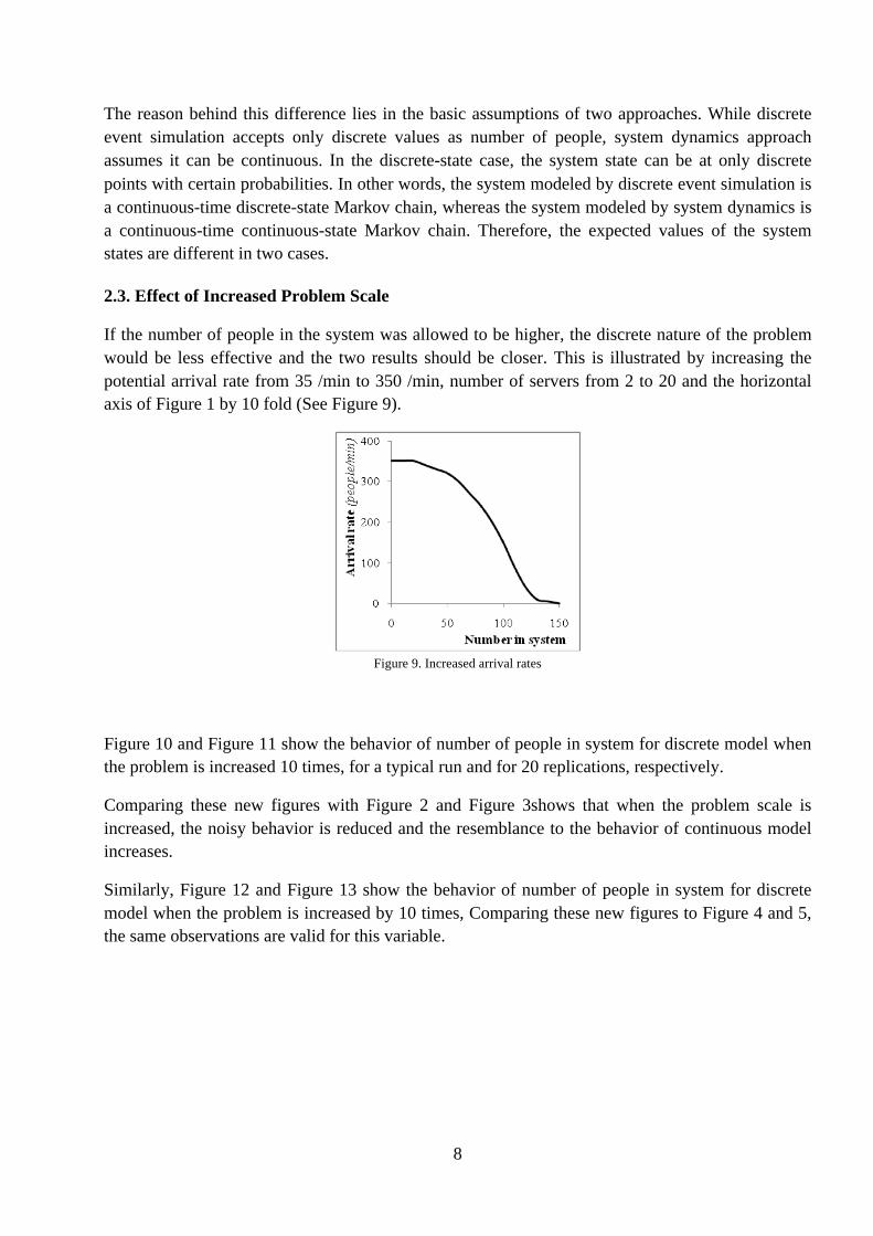
2.3. Effect of Increased Problem Scale

If the number of people in the system was allowed to be higher, the discrete nature of the problem

would be less effective and the two results should be closer. This is illustrated by increasing the

potential arrival rate from 35 /min to 350 /min, number of servers from 2 to 20 and the horizontal

axis of Figure 1 by 10 fold (See Figure 9).

Figure 9. Increased arrival rates

Figure 10 and Figure 11 show the behavior of number of people in system for discrete model when

the problem is increased 10 times, for a typical run and for 20 replications, respectively.

Comparing these new figures with Figure 2 and Figure 3shows that when the problem scale is

increased, the noisy behavior is reduced and the resemblance to the behavior of continuous model

increases.

Similarly, Figure 12 and Figure 13 show the behavior of number of people in system for discrete

model when the problem is increased by 10 times, Comparing these new figures to Figure 4 and 5,

the same observations are valid for this variable.

9

Figure 10. Behavior of number of people in system for discrete model when scale is increased, from a typical run

Figure 11. Behavior of number of people in system for discrete model when scale is increased (Average of 20 runs)

Figure 12. Behavior of average time spent in system for discrete model when scale is increased, from a typical run

10

Figure 13. Behavior of average time spent in system for discrete model when scale is increased (Average of 20 runs)

We can also find out what happens to the steady-state values of variables when the problem scale is

increased. The results are shown in Table 4. Comparing these results with the ones in Table 3, we

see that the per cent difference between continuous and discrete solutions for number in system

decreases from 5.0 % to 0.8 %. Similarly, the difference for the average time in system decreases

from 4.6 % to 0.8 %.

Table 4. Analytical results of steady-state values of variables when the problem scale is increased by 10 times

Thus, when the problem scale is increased, discrete and continuous models become much closer

both in behavior and in the steady-state values of variables.

3. System State Affects Arrival Rate after a Continuous Delay

Now, it is assumed that the mean arrival rate is a delayed function of the number of people in the

system, with an average delay time of 2 minutes. First-order information delay structure is selected

because in first order delay, the input (number of people in the system) shows its effect with an

exponential decreasing rate on the output (delayed number of people in the system), which is a

reasonable assumption. The delayed number of people in the system also can be regarded as the

perceived number of people in the system by the potential customers. They do not respond to every

change instantaneously but they react slowly. This is the continuous-delay case, since a change in

number in system influences the arrival rate gradually, distributed continuously over time. Note the

difference with discrete-delay in which a change in number in system shows any effect only after a

fixed period of time and instantaneously at that time. The discrete-delay case will be analyzed later.

11

3.1. Discrete Modeling of the System with a Continuous Delay

The first order information delay corresponds to exponential smoothing in discrete systems. So, in

discrete event simulation, a smoothed version of the number of system variable is used for

determining the probability of accepting potential customers. A new variable, delayed number in

system is defined and it is updated when an arrival or departure occurs. The number of people since

the last update of the variable is added by multiplying it with the duration since last update and the

smoothing constant (which is 1/DelayTime). The SIMAN code of the Arena model is in the

Appendix B.

The system is started with empty initial conditions. Figure 14 shows the behavior of number of

customers in the system in a typical discrete-event simulation run. Figure 15 shows the average

behavior of the same variable from 20 independent replications.

Figure 14. Behavior of number in system for discrete model with continuous delay, from a typical run

Figure 15. Behavior of number in system for discrete model with continuous delay (Average of 20 runs)

12

Figure 16 shows a typical run behavior of average time spent. Figure 17 shows the average behavior

in 20 replications. The initial sharp increase and overshoot followed by the pattern of approaching

the steady-state can be observed in both figures.

Figure 16. Behavior of average time spent in system for discrete model with continuous delay, from a typical run

Figure 17. Behavior of average time spent in system for discrete model with continuous delay (Average of 20 runs)

Table 5 presents the summary results of 50 500-hour-long replications after having discarded 30-

minutes warm-up period in each. Both average number in system and average time are higher

compared to the system without delay. This shows that introduction of delay increased the average

number of people and average time in the system.

Table 5. Steady state discrete event simulation results for the system with continuous delay

13

3.2. Continuous Modeling of the System with a Continuous Delay

A first order information delay structure is added to the existing model. The resulting equations are

in the Appendix B.

This model is a second order model with a negative loop between two stocks. Since all the loops are

balancing, the system can show a damping oscillatory behavior. Figure 18 shows number of people

in the system. Comparing this figure with Figure 15, we note the resemblance of the two dynamics.

The period and amplitude of the oscillations match. Naturally, the noise in discrete event simulation

prevents complete damping of the oscillations.

Figure 18. Behavior of number of people in system for system dynamics model with continuous delay

Figure 19 shows the behavior of average time in system. Like number of people in the system, it is

very similar to average waiting time for the discrete event simulation, which was shown in Figure

17.

Figure 19. Behavior of average time spent in system for system dynamics model with continuous delay

14

Table 6. Equilibrium points found by system dynamics simulation from the system with continuous delay

In this case, we cannot easily obtain analytical solutions for the steady-state values of variables.

However, we can use the results of simulations to comment on the similarity of two models in terms

of numerical values of variables in the long run. With enough precision, the results shown in

Table 5 and Table 6 reveal that the long-run values of the statistics are different in discrete event

simulation and system dynamics. Again, this can be explained by the discrete and continuous

natures of the two modeling approaches.


First note the difference between continuous and discrete modeling approaches by comparing

Figures 15 and 17 with Figures 18 and 19. The number of people in the system does not smooth out

in the discrete event simulation results unlike the system dynamics simulation. Also, the steady state

values are different as explained previously.

Now, the problem scale is increased 10 times by increasing servers to 20, the arrival pattern

following the rule shown in Figure 9. Figure 20 and Figure 21 show the behavior variables for the

discrete event simulation results of this scale-modified problem. Compare these figures with Figure

18 and Figure 19, keeping in mind that when the problem scale is increased only the numerical

values of the vertical axis of these two figures will change. The behaviors of variables for the two

simulation approaches become closer to each other, compared to Figures 15 and 17.

Figure 20. Behavior of number of people in system for discrete model with continuous delay when scale is increased

(A typical run on the left, average of 20 runs on the right)

Figure 21. Behavior of average time spent in system for discrete model with continuous delay when scale is increased


15

4. System State Affects Arrival Rate after a Discrete Delay

In this case, the continuous delay structure of previous section is turned into a discrete delay with a

delay time of 2 minutes. An arriving customer observes the state of the system exactly two minutes

ago and decides to enter or not accordingly.

4.1. Discrete Modeling of the System with a Discrete Delay

As a modification to the model, a variable is added indicating the number in system 2 minutes ago.

The SIMAN code of the modified model is in the Appendix B.

The system is started with empty initial conditions. Figure 22 shows a typical and the average

behavior of number of people in the system. In the long run, number in system shows a non-

damping oscillation throughout the simulation. Therefore it is not possible to find constant steady-

state results.

Figure 22. Behavior of number in system for discrete model with discrete delay


Figure 23 shows the behavior of average time spent in system. Since this is an accumulated

variable, it eventually damps out, but the oscillations are observable for a longer period compared to

the continuous-delay case (See Figure 16 and Figure 17). Also, the steady-state value of this

variable for discrete-delay case is higher than that for continuous-delay case.

Figure 23. Behavior of average time spent in system for discrete model with discrete delay


4.2. Continuous Modeling of the Discrete-Delay Case

Discrete delay is modeled in system dynamics by a conveyor structure with a transit time of

2 minutes. This discrete-delayed number in system is used as input of the effect function on the

arrival rate. The equations of the system dynamics model are in the Appendix B.

16

Figure 24 demonstrates the behavior of number of people from system dynamics model of the

system with discrete information delay. There is a constant oscillation with a peak value of 36 and a

period about 6 minutes. Putting side by side this figure with Figure 22 illustrates a basic similarity

of two behavior patterns. The far right side of Figure 22 has oscillations with smaller amplitude,

since it is the average of 20 runs. The behaviors of individual runs have oscillations with amplitudes

comparable to the size of oscillations of system dynamics model.

Figure 24. Behavior of number in system, from system dynamics model with discrete delay

Figure 25 demonstrates the behavior of average time in system variable for the same case. The

steady-state value for system dynamics model is significantly lower than the value for discrete event

simulation. This is due to the fact that the number of people in system is lower compared to the

discrete event simulation.

Figure 25. Behavior of average time spent in system for system dynamics model with discrete delay


Figure 26 and Figure 27 show the behavior of system variables when the problem scale is increased

as described in Section 2.3. Comparing these behaviors with the ones in Figure 22-Figure 23 and

with Figure 24-25, we see that the increasing the problem scale makes the behavior closer to

behavior of continuous model (although some difference still remains).

17

Figure 26. Behavior of number of people in system for discrete model with discrete delay when scale is increased


Figure 27. Behavior of average time spent in system for discrete model with discrete delay when scale is increased


5. Conclusion

In this study, discrete and continuous simulations are compared in terms of dynamic behaviors and

steady-state values of two main variables of a M/M/2 queuing system with crowd-dependent arrival

rate. Although the M/M/2 queuing system is a discrete-state system by definition, it is also modeled

by continuous system dynamics approach, by making some assumptions. In a series of experiments,

the effects of following factors are tested: the problem scale, the existence and type of the delay in

the feedback path from the crowd level to arrival rate.

Increasing the problem scale is achieved by increasing the arrival rate and number of servers by ten

fold. This increased scale renders the discrete nature of problem less significant. Therefore, the

discrete simulation comes closer to the continuous simulation, which reveals itself as decreased

noise in the output and values closer to continuous simulation results in the steady-state.

In the experiments, the number of people in the system affects the arrival rate i- with no delay,

ii- with continuous delay and iii- with discrete delay. Introducing the continuous delay yielded

damping oscillations in the number of people variable, for both discrete and continuous simulations.

System dynamics models yielded clearer dynamic patterns since they do not include noise.

Changing the delay type from continuous to discrete, changed the behavior from damping to non-

damping oscillations. The resemblance of the basic behavior patterns between two simulation

approaches is preserved in trials with different delay times and problem scales. These results

support the usability of continuous simulation for approximating the behavior patterns and

18

equilibrium levels of system variables in queuing systems. We also verify our findings by some

analytical results, in cases where they are obtainable. Clearly, a more thorough and comprehensive

study is needed to arrive at more concrete conclusions on the potential role of continuous simulation

in queuing systems. For instance, our experiments show that when there is a discrete delay on the

feedback path from the system state (crowd level) back to the arrivals, significant differences occur

between the equilibrium levels of time spent in system from discrete and continuous simulations.

Although continuous simulation can be useful in obtaining the dynamic behaviors, it is not wise to

use the numerical output values of system dynamics simulation as estimates of the queuing system

parameters, due to the fact that system dynamics models include assumptions that reduce their

capability of providing such estimates.

There are some difficulties in trying to perform an exact comparison of two simulation approaches

to the system under consideration. Due to difference in the continuity assumptions of two

approaches it impossible to model the same physical phenomena identically. Discrete event

simulation is mainly oriented towards finding statistical estimates for equilibrium values of output

variables, without much interest in dynamic behaviors. Indeed, the notion of dynamic pattern is not

very clear in discrete event simulation, the plots of variables being generally too noisy. At the other

extreme, averaging of variable values may smooth out most patterns, making it impossible again to

detect meaningful behaviors. System dynamics approach, on the other hand, requires replacement

of random events with their deterministic means (flows), which is a handicap if one is interested in

finding precise statistical estimates of steady-state values of variables.

References

Crespo-Márquez, A., R. R. Usano and R. D. Aznar, 1993, "Continuous and Discrete Simulation in a

Production Planning System. A Comparative Study", Proceedings of International System

Dynamics Conference, Cancun, Mexico, p. 58, The System Dynamics Society.

isee systems, 2007, STELLA, v. 9.0, Lebanon, NH, USA.

Rockwell Automation, 2006, Arena, v. 11.00, Wexford, PA, USA.

Roy, R. K. and P. K. J. Mohapatra, 1993, "A System Dynamics Based Methodology for

Numerically Solving Transient Behaviour of Queuing Systems", Proceedings of International

System Dynamics Conference, Cancun, Mexico, p. 408, The System Dynamics Society.

Sweetser, A., 1999, "A Comparison of System Dynamics (SD) and Discrete Event Simulation

(DES)", Proceedings of 17th International Conference of the System Dynamics Society and 5th

Australian & New Zealand Systems Conference, Wellington, New Zealand, 20-23 July,

p. 8, The System Dynamics Society.

Welch, P. D., 1981, On the problem of the initial transient in steady-state simulation, IBM Watson

Research Center, Yorktown Heights, NY, USA.

19

Appendix A: Analytical calculations of statistics for discrete state space model

The system is modeled as continuous time Markov chain. The limiting probabilities of being at each

state are found by solving the following balance equations.

35 P0 = 10 P1

45 P0 = 20 P2 + 35 P1

55 P1 = 20 P3 + 35 P2

54 P2 = 20 P4 + 35 P3

53 P3 = 20 P5 + 34 P4

52 P4 = 20 P6 + 33 P5

50 P5 = 20 P7 + 32 P6

47 P6 = 20 P8 + 30 P7

44 P7 = 20 P9 + 27 P8

40 P8 = 20 P10 + 24 P9

35 P9 = 20 P11 + 20 P10

29 P10 = 20 P12 + 15 P11

24 P11 = 20 P13 + 9 P12

21 P12 = 20 P14 + 4 P13

20.5 P13 = 20 P15 + P14

Rearranging gives,

P1 = 3.5 P0

P2 = 2.25 P1 – 1.75 P0

P3 = 2.75 P2 – 1.75 P1

P4 = 2.7 P3 – 1.75 P2

P5 = 2.65 P4 – 1.7 P3

P6 = 2.6 P5 – 1.65 P4

P7 = 2.5 P6 – 1.6 P5

P8 = 2.35 P7 – 1.5 P6

P9 = 2.2 P8 – 1.35 P7

P10 = 2 P9 – 1.2 P8

P11 = 1.75 P10 – 1 P9

P12 = 1.45 P11 – 0.75 P10

P13 = 1.2 P12 – 0.45 P11

P14 = 1.05 P13 – 0.2 P12

P15 = 1.025 P14 – 0.05 P13

In terms of probability of that system is empty; the probabilities of other states are;

P0 = 1 P0

P1 = 3.5 P0

P2 = 6.125 P0

P3 = 10.7188 P0

P4 = 18.2219 P0

P5 = 30.0661 P0

P6 = 48.1058 P0

P7 = 72.1586 P0

P8 = 97.4141 P0

P9 = 116.897 P0

P10 = 116.897 P0

P11 = 87.6727 P0

P12 = 39.4527 P0

P13 = 7.8905 P0

P14 = 0.3945 P0

P15 = 0.0099 P0

Since the total probability is 1,

P0 = 0.00152

All probabilities can be calculated by using the above equations. The results are summarized in the

following table.

20

We can calculate basic statistics as follows;

Using Little’s formula,

Appendix B: Model Equations

The SIMAN code of the Arena model

Code for the model without delay: ENTITIES: Customer,Picture.Person; RESOURCES: Server,Capacity(2); QUEUES: ServiceQ,FirstInFirstOut; VARIABLES: NumberInSystem; ATTRIBUTES: ArrivalTime; TABLES:

PercentAccepted,0,1,100,100,100,97.1,94.3,91.4,85.7,77.1,68.6,57.1,42.9,25.7,11.4,2.9,1.4,0; TALLIES: Time in System; DSTATS: NumberInSystem, Number in System; OUTPUTS: DAVG(Number in System),,Average Number in System: TAVG(Time in System),,Average Time in System; 0$ CREATE, 1,0,Customer:EXPO(1/35):MARK(ArrivalTime); 1$ BRANCH, 1: With,TF(PercentAccepted,NumberInSystem)/100,enter: Else, donotenter; donotenter DISPOSE;

enter ASSIGN: NumberInSystem = NumberInSystem + 1;

4$ QUEUE, ServiceQ; 5$ SEIZE, 1: Server,1; 6$ DELAY: EXPO(1/10); 7$ RELEASE: Server,1; 9$ ASSIGN: NumberInSystem = NumberInSystem - 1; 10$ TALLY: Time in System, TNOW - ArrivalTime, 1; 8$ DISPOSE;

Code for the model with continuous delay: VARIABLES: DelayTime,2: Last Time of Change in Number in System; Delayed Number in System;

21

0$ CREATE, 1,0,Customer:EXPO(1/35):MARK(ArrivalTime); 10$ ASSIGN: Delayed Number in System=

NumberInSystem*(TNOW - Last Time of Change in Number in System)/DelayTime+(1-((TNOW - Last Time of Change in Number in System)/DelayTime))*Delayed Number in System:

Last Time of Change in Number in System=TNOW; 1$ BRANCH, 1:

With,TF(PercentAccepted,Delayed Number in System)/100,enter: Else,donotenter; donotenter DISPOSE; enter ASSIGN: Delayed Number in System=


NumberInSystem=NumberInSystem + 1: Last Time of Change in Number in System=TNOW; 2$ QUEUE, ServiceQ; 3$ SEIZE, 1: Server,1; 4$ DELAY: EXPO(1/10); 5$ RELEASE: Server,1; 7$ ASSIGN: Delayed Number in System=


NumberInSystem=NumberInSystem - 1: Last Time of Change in Number in System=TNOW; 8$ TALLY: Time in System,TNOW - ArrivalTime,1; 6$ DISPOSE;

Code for the model with discrete delay:

Last Time of Change in Number in System removed

0$ CREATE, 1,0,Customer:EXPO(1/35):MARK(ArrivalTime):NEXT(1$); 1$ BRANCH, 1: With,TF(PercentAccepted,Delayed Number in System)/100,enter: Else,donotenter; donotenter DISPOSE: No; enter ASSIGN: NumberInSystem=NumberInSystem + 1; 20$ DUPLICATE: 1,incdelayed; 2$ QUEUE, ServiceQ; 3$ SEIZE, 1,ValueAdded: Server,1; 4$ DELAY: EXPO(1/10); 5$ RELEASE: Server,1; 7$ ASSIGN: NumberInSystem=NumberInSystem - 1; 24$ DUPLICATE: 1,decrdelayed; 8$ TALLY: Time in System,TNOW - ArrivalTime,1; 6$ DISPOSE: No; incdelayed DELAY: DelayTime,,Other:NEXT(21$); 21$ ASSIGN: Delayed Number in System=Delayed Number in System + 1; 23$ DISPOSE: No; decrdelayed DELAY: DelayTime,,Other:NEXT(25$); 25$ ASSIGN: Delayed Number in System=Delayed Number in System - 1; 27$ DISPOSE: No;

STELLA equations of the system dynamics model

Equations for the model without delay: Number_in_system(t) = Number_in_system(t - dt) + (Arrival_rate - Service_rate) * dt INIT Number_in_system = 0 Arrival_rate = Potential_arrival_rate * (Percentage_of_potential_arrivals_enter/100) Service_rate = Number_of_Busy_Servers * One_Server's_Service_Rate Number_of_Busy_Servers = MIN(Number_in_system*Servers_used_per_person, Total_number_of_servers) One_Server's_Service_Rate = 10 Potential_arrival_rate = 35 Servers_used_per_person = 1 Total_number_of_servers = 2

22

Percentage_of_potential_arrivals_enter = GRAPH(Number_in_system) (0,100),(1,100),(2,100),(3,97.1),(4,94.3),(5,91.4),(6,85.7),(7,77.1),(8,68.6),(9,57.1),(10,42.9), (11,25.7),(12,11.4),(13,2.86),(14,1.43),(15,0) Total_Time_in_System(t) = Total_Time_in_System(t - dt) + (Time_in_System) * dt INIT Total_Time_in_System = 0 Time_in_System = Number_in_system/(0.0000001+Service_rate) Avg_time_in_system = Total_Time_in_System/(TIME+DT)

Equations for the model with continuous delay:

Number_in_system(t) = Number_in_system(t - dt) + (Arrival_rate - Service_rate) * dt INIT Number_in_system = 0 Arrival_rate = Potential_arrival_rate * (Percentage_of_potential_arrivals_enter/100) Service_rate = Number_of_Busy_Servers * One_Server's_Service_Rate Number_of_Busy_Servers = MIN(Number_in_system*Servers_used_per_person, Total_number_of_servers) One_Server's_Service_Rate = 10 Potential_arrival_rate = 35 Servers_used_per_person = 1 Total_number_of_servers = 2 Delayed_number_in_system(t) = Delayed_number_in_system(t - dt) + (Change_in_delayed_nis) * dt INIT Delayed_number_in_system = 0 Change_in_delayed_nis = (Number_in_system-Delayed_number_in_system)/Average_delay Average_delay = 2 Percentage_of_potential_arrivals_enter = GRAPH(Delayed_number_in_system) (0,100),(1,100),(2,100),(3,97.1),(4,94.3),(5,91.4),(6,85.7),(7,77.1),(8,68.6),(9,57.1),(10,42.9), (11,25.7),(12,11.4),(13,2.86),(14,1.43),(15,0)

Equations for the model with discrete delay:

Number_in_system(t) = Number_in_system(t - dt) + (Arrival_rate - Service_rate) * dt INIT Number_in_system = 0 Arrival_rate = Potential_arrival_rate * (Percentage_of_potential_arrivals_enter/100) Service_rate = Number_of_Busy_Servers * One_Server's_Service_Rate Number_of_Busy_Servers = MIN(Number_in_system*Servers_used_per_person, Total_number_of_servers) One_Server's_Service_Rate = 10 Potential_arrival_rate = 35 Servers_used_per_person = 1 Total_number_of_servers = 2 NIS_during_delay(t) = NIS_during_delay(t-dt) + (Change_in_delayed_nis-Delayed_number_in_system) * dt INIT NIS_during_delay = 0 TRANSIT TIME = 2 INFLOW LIMIT = INF CAPACITY = INF Change_in_delayed_nis = Number_in_system Delayed_number_in_system = CONVEYOR OUTFLOW

Documents

Discrete vs. Continuous Simulation: When Does It Matter? · model is built with the simulation package Arena (Rockwell Automation, 2006). The SIMAN code of the Arena model is in the