Discrete Time Series Analysis With ARMA Models

Discrete Time Series Analysis with ARMA Models

Veronica Sitsofe Ahiati ([email protected])African Institute for Mathematical Sciences (AIMS)

Supervised by Tina MarquardtMunich University of Technology, Germany

June 6, 2007

Abstract

The goal of time series analysis is to develop suitable models and obtain accurate predictions formeasurements over time of various kinds of phenomena, like yearly income, exchange rates ordata network traffic. In this essay we review the classical techniques for time series analysis whichare linear time series models; the autoregressive models (AR), the moving average models (MA)and the mixed autoregressive moving average models (ARMA). Time series analysis can be usedto extract information hidden in data. By finding an appropriate model to represent the data,we can use it to predict future values based on the past observations. Furthermore, we considerestimation methods for AR and MA processes, respectively.

i

Contents

Abstract i

List of Figures iii

1 A Brief Overview of Time Series Analysis 1

1.1 Introduction . . . . . . . . . . . . . . . . . . . . . . . . . . . . . . . . . . . . 1

1.2 Examples and Objectives of Time Series Analysis . . . . . . . . . . . . . . . . . 1

1.2.1 Examples of Time Series Analysis . . . . . . . . . . . . . . . . . . . . . 1

1.2.2 Objectives of Time Series Analysis . . . . . . . . . . . . . . . . . . . . 2

1.3 Stationary Models and the Autocorrelation Function . . . . . . . . . . . . . . . 3

1.4 Removing Trend and Seasonal Components . . . . . . . . . . . . . . . . . . . . 8

2 ARMA Processes 9

2.1 Definition of ARMA Processes . . . . . . . . . . . . . . . . . . . . . . . . . . . 9

2.1.1 Causality and Invertibility of ARMA Processes . . . . . . . . . . . . . . 10

2.2 Properties of ARMA Processes . . . . . . . . . . . . . . . . . . . . . . . . . . 13

2.2.1 The Spectral Density . . . . . . . . . . . . . . . . . . . . . . . . . . . 13

2.2.2 The Autocorrelation Function . . . . . . . . . . . . . . . . . . . . . . . 14

3 Prediction 19

3.1 The Durbin-Levinson Algorithm . . . . . . . . . . . . . . . . . . . . . . . . . . 20

4 Estimation of the Parameters 21

4.1 The Yule-Walker Equations . . . . . . . . . . . . . . . . . . . . . . . . . . . . 21

4.2 The Durbin-Levinson Algorithm . . . . . . . . . . . . . . . . . . . . . . . . . . 24

4.3 The Innovations Algorithm . . . . . . . . . . . . . . . . . . . . . . . . . . . . . 25

5 Data Example 27

6 Conclusion 31

ii

A Programs for Generating the Various Plots 32

A.1 Code for plotting data . . . . . . . . . . . . . . . . . . . . . . . . . . . . . . . 32

A.2 Code for plotting the autocorrelation function of MA(q) process . . . . . . . . . 33

A.3 Code for plotting the partial autocorrelation function of MA(1) process . . . . . 34

A.4 Code for Plotting the Spectral Density Function of MA(1) process . . . . . . . . 34

Bibliography 37

iii

List of Figures

1.1 Examples of time series . . . . . . . . . . . . . . . . . . . . . . . . . . . . . . 2

1.2 The sample acf of the concentration of CO2 in the atmoshpere, see Remark 1.14 5

1.3 Simulated stationary white noise time series . . . . . . . . . . . . . . . . . . . . 6

2.1 The acf for MA(1) with θ = −0.9 . . . . . . . . . . . . . . . . . . . . . . . . . 16

2.2 The pacf for MA(1) with θ = −0.9 . . . . . . . . . . . . . . . . . . . . . . . . 16

2.3 The spectral density of MA(1) with θ = −0.9 . . . . . . . . . . . . . . . . . . . 16

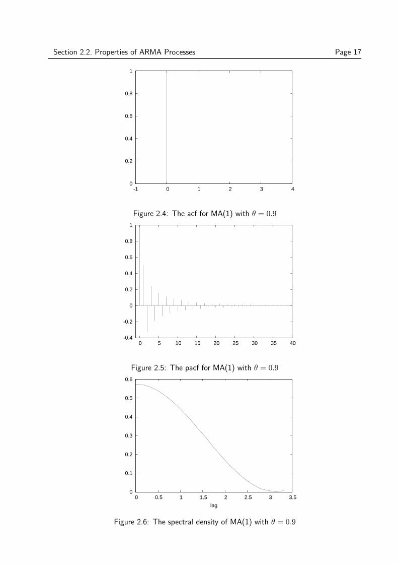
2.4 The acf for MA(1) with θ = 0.9 . . . . . . . . . . . . . . . . . . . . . . . . . . 17

2.5 The pacf for MA(1) with θ = 0.9 . . . . . . . . . . . . . . . . . . . . . . . . . 17

2.6 The spectral density of MA(1) with θ = 0.9 . . . . . . . . . . . . . . . . . . . . 17

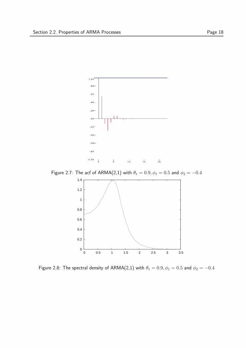
2.7 The acf of ARMA(2,1) with θ1 = 0.9, φ1 = 0.5 and φ2 = −0.4 . . . . . . . . . 18

2.8 The spectral density of ARMA(2,1) with θ1 = 0.9, φ1 = 0.5 and φ2 = −0.4 . . . 18

5.1 The plot of the original series {Xt} of the SP500 index . . . . . . . . . . . . . 27

5.2 The acf and the pacf of Figure 5.1 . . . . . . . . . . . . . . . . . . . . . . . . 27

5.3 The differenced mean corrected series {Yt} in Figure 5.1 . . . . . . . . . . . . . 28

5.4 The acf and the pacf of Figure 5.3 . . . . . . . . . . . . . . . . . . . . . . . . 28

5.5 The plot of the acf and the pacf of the residuals . . . . . . . . . . . . . . . . . 29

5.6 The spectral density of the fitted model . . . . . . . . . . . . . . . . . . . . . . 30

5.7 The plot of the forecasted values with 95% confidence interval . . . . . . . . . . 30

iv

1. A Brief Overview of Time SeriesAnalysis

1.1 Introduction

Time, in terms of years, months, days, or hours is a device that enables one to relate phenomenato a set of common, stable reference points. In making conscious decisions under uncertainty,we all make forecasts. Almost all managerial decisions are based on some form of forecast.In our quest to know the consequence of our actions, a mathematical tool called time seriesis developed to help guiding our decisions. Essentially, the concept of a time series is basedon historical observation. It involves examining past values in order to try to predict those inthe future. In analysing time series, successive observations are usually not independent, andtherefore, the analysis must take into account the time order of the observation.

The classical method used to investigate features in a time series in the time domain is tocompute the covariance and correlation function and in the frequency domain is by frequencydecomposition of the time series which is achieved by a way of Fourier analysis.

In this chapter, we will give some examples of time series and discuss some of the basic conceptsof time series analysis including stationarity, the autocovariance and the autocorrelation functions.The general autoregressive moving average process (ARMA), its causality, invertibility conditionsand properties will be discussed in Chapter 2. In Chapter 3 and 4, we will give a general overviewof prediction and estimation of ARMA processes, respectively. In particular, we will consider adata example in Chapter 5.

1.2 Examples and Objectives of Time Series Analysis

1.2.1 Examples of Time Series Analysis

Definition 1.1 A time series is a collection of observations {xt}t∈T made sequentially in timet. A discrete-time time series (which we will work with in this essay) is one in which the set Tof times at which observations are made is discrete e.g. T = {1, 2, . . . , 12} and a continuous-time time series is obtained when observations are made continuously over some time intervale.g. T = [0, 1] [BD02].

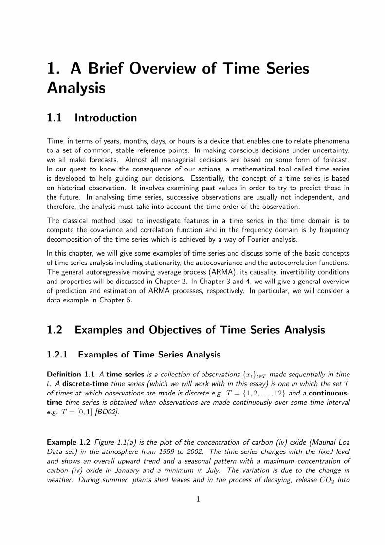
Example 1.2 Figure 1.1(a) is the plot of the concentration of carbon (iv) oxide (Maunal LoaData set) in the atmosphere from 1959 to 2002. The time series changes with the fixed leveland shows an overall upward trend and a seasonal pattern with a maximum concentration ofcarbon (iv) oxide in January and a minimum in July. The variation is due to the change inweather. During summer, plants shed leaves and in the process of decaying, release CO2 into

1

Section 1.2. Examples and Objectives of Time Series Analysis Page 2

310

320

330

340

350

360

370

380

0 10 20 30 40 50 60 70 80 90

(a) The plot of the concentration of CO2

in the atmosphere

-1

-0.8

-0.6

-0.4

-0.2

0

0.2

0.4

0.6

0.8

1

0 20 40 60 80 100 120 140 160 180 200

signalsignal with noise

(b) Example of a signal plus noise dataplot

Figure 1.1: Examples of time series

the atmosphere and during winter, plants make use of CO2 in the atmosphere to grow leavesand flowers. A time series with these characteristics is said to be non-stationary in both meanand variance.

Example 1.3 Figure (1.1(b)) shows the graph of {Xt} = Nt sin(ωt+θ), t = 1, 2, ..., 200, where{Nt}t=1,2,...,200 is a sequence of independent normal random variables with zero mean and unitvariance, and sin(ωt+ θ) is the signal component. There are many approaches to determine theunknown signal components given the data Xt and one such approach is smoothing. Smoothingdata removes random variation and shows trends and cyclic components. The series in thisexample is called signal plus noise.

Definition 1.4 A time series model for the observed data {xt} is a specification of the jointdistributions of a sequence of random variables {Xt}t∈T of which Xt = xt is postulated to be arealization. We also refer to the stochastic process {Xt}t∈T as time series.

1.2.2 Objectives of Time Series Analysis

A modest objective of any time series analysis is to provide a concise description of the pastvalues of a series or a description of the underlying process that generates the time series. A plotof the data shows the important features of the series such as the trend, seasonality, and anydiscontinuities. Plotting the data of a time series may suggest a removal of seasonal componentsin order not to confuse them with long-term trends, known as seasonal adjustment. Otherapplications of time series models include the separation of noise from signals, forecasting futurevalues of a time series using historical data and testing hypotheses. When time series observationsare taken on two or more variables, it may be possible to use the variation in one time series toexplain the variation of the other. This may lead to a deeper understanding of the mechanismgenerating the given observations [Cha04].

In this essay, we shall concentrate on autoregressive moving average (ARMA) processes as aspecial class of time series models most commonly used in practical applications.

Section 1.3. Stationary Models and the Autocorrelation Function Page 3

1.3 Stationary Models and the Autocorrelation Function

Definition 1.5 The mean function of a time series {Xt} with E(X2t ) <∞ is

µX(t) = E(Xt), t ∈ Z,

and the covariance function is

γX(r, s) = cov(Xr, Xs) = E[(Xr − µX(r))(Xs − µX(s))]

for all r, s ∈ Z.

Definition 1.6 A time series {Xt}t∈T is weakly stationary if both the mean

µX(t) = µX ,

and for each h ∈ Z, the covariance function

γX(t+ h, t) = γX(h)

are independent of time t.

Definition 1.7 A time series {Xt} is said to be strictly stationary if the joint distributions of(X1, . . . , Xn) and (X1+h, . . . , Xn+h) are the same for all h ∈ Z and n > 0.

Definitions 1.6 and 1.7 imply that if a time series {Xt} is strictly stationary and satisifies thecondition E(X2

t ) <∞, then {Xt} is also weakly stationary. Therefore we assume that E(X2t ) <

∞. In this essay, stationary refers to weakly stationary.

For a single variable, the covariance function of a stationary time series {Xt}t∈T is defined as

γX(h) = γX(h, 0) = γX(t+ h, t),

where γX(·) is the autocovariance function and γX(h) its value at lag h.

Proposition 1.8 Every Gaussian weakly stationary process is strictly stationary.

Proof 1.9 The joint distributions of any Gaussian stochastic process are uniquely determinedby the second order properties, i.e., by the mean µ and the covariance matrix. Hence, since theprocess is weakly stationary, the second order properties do not depend on time t (see Definition1.6). Therefore, it is strictly stationary.

Definition 1.10 The autocovariance function (acvf) and the autocorrelation function(acf) of a stationary time series {Xt} at lag h are given respectively as:

γX(h) = cov(Xt+h, Xt), (1.1)

and

ρX(h) =γX(h)

γX(0)= cor(Xt+h, Xt). (1.2)


The linearity property of covariances is that, if E(X2), E(Y 2) and E(Z2) <∞, and a and b arereal constants, then

cov(aX + bY, Z) = acov(X,Z) + bcov(Y, Z) (1.3)

Proposition 1.11 If γX is the autocovariance function of a stationary process {Xt}t∈Z, then

(i) γX(0) ≥ 0,

(ii) |γX(h)| ≤ γX(0), ∀ h ∈ Z,

(iii) γX(h) = γX(−h).

Proof 1.12 (i) From var(Xt) ≥ 0,

γX(0) = cov(Xt, Xt) = E(Xt − µX)(Xt − µX) = E(X2t ) − µ2

X = var(Xt) ≥ 0.

(ii) From Cauchy-Schwarz inequality,

|γX(h)| = |cov(Xt+h, Xt)| = |E(Xt+h − µX)(Xt − µX)|≤ [E(Xt+h − µX)2]

1

2 [E(Xt − µX)2]1

2 ≤ γX(0)

(iii) γX(h) = cov[Xt, Xt+h] = cov[Xt−h, Xt] = γX(−h)since {Xt} is stationary.

Definition 1.13 The sample mean of a time series {Xt} with x1, . . . , xn as its observations is

x =1

n

n∑

t=1

xt,

and the sample autocovariance function and the sample autocorrelation function arerespectively given as

γ̂(h) =1

n

n−|h|∑

t=1

(xt+|h| − x)(xt − x),

and

ρ̂(h) =γ̂(h)

γ̂(0),

where −n < h < n.

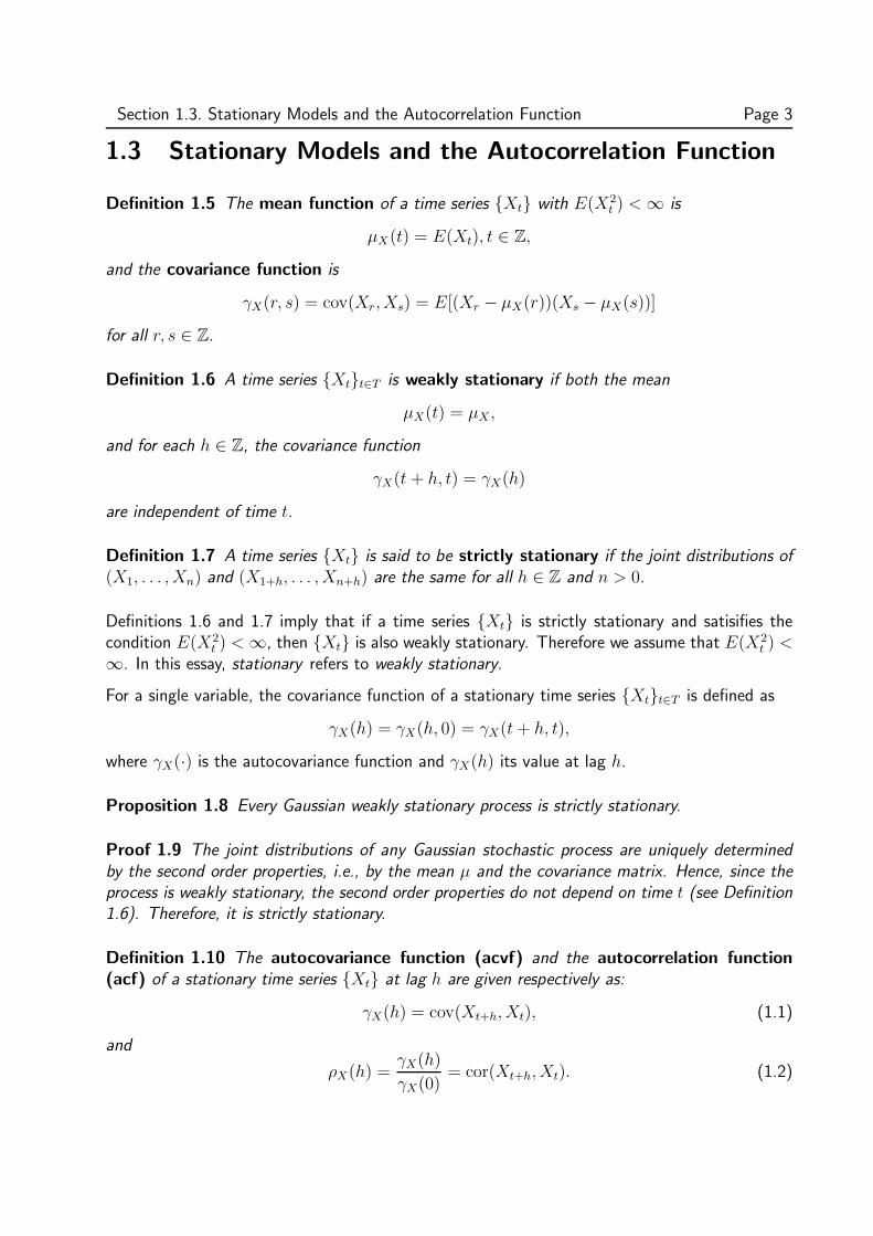
Remark 1.14 The sample autocorrelation function is useful in determining the non-stationarityof data since it exhibits the same features as the plot of the data. An example is shown in Figure1.2. It can be seen that the plot of the acf exhibits the same oscillations, i.e. seasonal effects, asthe plot of the data.


Figure 1.2: The sample acf of the concentration of CO2 in the atmoshpere, see Remark 1.14

Definition 1.15 A sequence of independent random variables X1, ..., Xn, in which there is notrend or seasonal component and the random variables are identically distributed with mean zerois called iid noise.

Example 1.16 If the time series {Xt}t∈Z is iid noise and E(X2t ) = σ2 < ∞, then the mean of

{Xt} is independent of time t, since E(Xt) = 0 for all t and

γX(t+ h, t) =

{σ2, if h = 0,

0, if h 6= 0

is independent of time. Hence iid noise with finite second moments is stationary.

Remark 1.17 {Xt} ∼ IID(0, σ2) indicates that the random variablesXt, t ∈ Z are independentand identically distributed, each with zero mean and variance σ2.

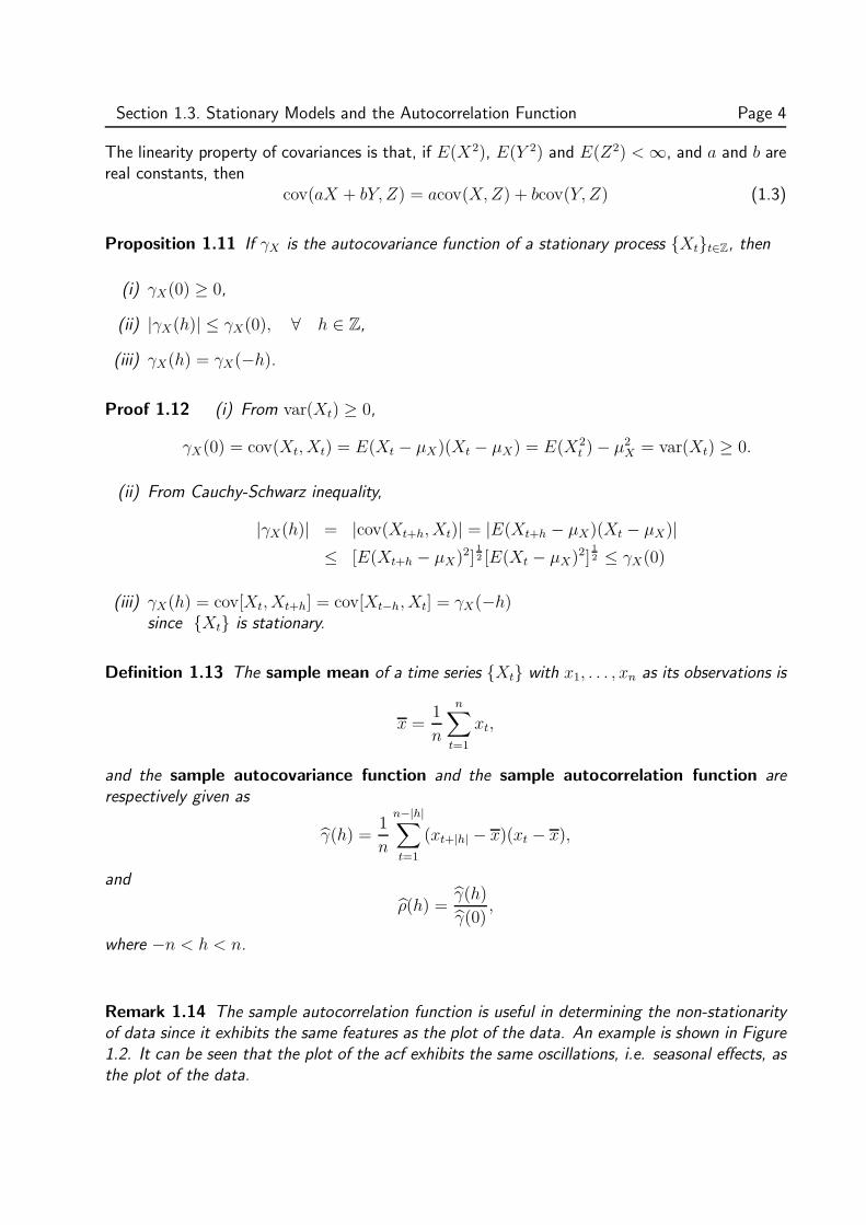
Example 1.18 White noise is a sequence {Xt} of uncorrelated random variables such thateach random variable has zero mean and a variance of σ2. We write {Xt} ∼ WN(0, σ2). Then{Xt} is stationary with the same covariance function as the iid noise. A plot of white noise timeseries is shown in Figure 1.3.

Example 1.19 A sequence of iid random variables {Xt}t∈N with

P (Xt = 1) = p,

andP (Xt = −1) = 1 − p

is called a binary process, e.g. tossing a coin with p = 12.


-3

-2

-1

0

1

2

3

0 50 100 150 200

Figure 1.3: Simulated stationary white noise time series

A time series {Xt} is a random walk with {Zt} a white noise, if

Xt = Xt−1 + Zt.

Starting the process at time t = 0 and X0 = 0,

Xt = Zt + Zt−1 + . . .+ Z1,

E(Xt) = E(Zt + Zt−1 + . . .+ Z1) = 0.

var(Xt) = E(X2t )

= E[(Zt + Zt−1 + . . .+ Z1)

2]

= E(Zt)2 + E(Zt−1)

2 + . . .+ E(Z1)2 (independence)

= tσ2.

The time series {Xt} is non stationary since the variance increases with t.

Example 1.20 A time series {Xt} is a first order moving average, MA(1), if

Xt = Zt + θZt−1, t ∈ Z, (1.4)

where {Zt} ∼ WN(0, σ2) and |θ| < 1.From Example 1.16,

E(Xt) = E(Zt + θZt−1)

= E(Zt) + θE(Zt−1) = 0,

E(XtXt+1) = E [(Zt + θZt−1)(Zt+1 + θZt)]

= E[ZtZt+1 + θZ2

t + θZt−1Zt+1 + θ2ZtZt+1

]

= E(ZtZt+1) + θE(Z2t ) + θE(Zt−1Zt+1) + θ2E(ZtZt+1)

= θσ2,


and

E(X2t ) = E(Zt + θZt−1)

2

= E(Z2t ) + 2θE(Zt)E(Zt−1) + θ2E(Z2

t−1)

= σ2(1 + θ2) <∞.

Hence

γX(t+ h, t) = cov(Xt+h, Xt) = E(Xt+h, Xt)

=

σ2(1 + θ2), if h = 0,

σ2θ, if h = ±1,

0, if | h |> 1.

Since γX(t+ h, t) is independent of t, {Xt} is stationary.

The autocorrelation function is given as:

ρX(h) = cor(Xt+h, Xt) =γX(h)

γX(0)

=

1, if h = 0,θ

1 + θ2, if h = ±1,

0, if | h |> 1.

Example 1.21 A time series {Xt} is a first-order autoregressive or AR(1) process if

Xt = φXt−1 + Zt, t ∈ Z, (1.5)

where {Zt} ∼ WN(0, σ2), | φ |< 1, and for each s < t, Zt is uncorrelated with Xs.

γX(0) = E(X2t )

= E [(φXt−1 + Zt)(φXt−1 + Zt)]

= φ2E(X2t−1) + E(Z2

t )

= φ2γX(0) + σ2.

Solving for γX(0),

γX(0) =σ2

1 − φ2.

Since Zt and Xt−h are uncorrelated, cov(Zt, Xt−h) = 0, ∀ h 6= 0.The autocovariance function at lag h > 0 is

γX(h) = cov(Xt, Xt−h)

= cov(φXt−1 + Zt, Xt−h) from Equation 1.3

= φcov(Xt−1, Xt−h) + cov(Zt, Xt−h) = φcov(Xt−1, Xt−h)

= φcov(φXt−2 + Zt−1, Xt−h) = φ2cov(Xt−2, Xt−h)

Continuing this procedure,

γX(h) = φhγX(0), h ∈ Z+

γX(h) = φ|h|γX(0), h ∈ Z,

Section 1.4. Removing Trend and Seasonal Components Page 8

due to symmetry of γX(h) (see Proposition 1.11 (iii)). Therefore, the autocorrelation function isgiven as

ρX(h) =γX(h)

γX(0)=φ|h|γX(0)

γX(0)= φ|h|, h ∈ Z. (1.6)

1.4 Removing Trend and Seasonal Components

Many time series that arise in practice are non-stationary but most available techniques are foranalysis of stationary time series. In order to make use of these techniques, we need to modifyour time series so that it is stationary. An example of a non-stationary time series is given inFigure 1.1(a). By a suitable transformation, we can transform a non-stationary time series intoan approximately stationary time series. Time series data are influenced by a variety of factors.It is essential that such components are decomposed out of the raw data. In fact, any timeseries can be decomposed into a trend component mt, a seasonal component st with knownperiod, and a random noise Yt as

Xt = mt + st + Yt, t ∈ Z. (1.7)

For nonseasonal models with trend, Equation (1.7) becomes

Xt = mt + Yt, t ∈ Z. (1.8)

For a nonseasonal time series, first order differencing is usually sufficient to attain apparentstationarity so that the new series (y1, . . . , yn) is formed from the original series (x1, . . . , xn) byyt = xt+1 − xt = ∇xt+1. Second order differencing is required using the operator ∇2, where∇2xt+2 = ∇xt+2 −∇xt+1 = xt+2 − 2xt+1 + xt. The concept of backshift operator B helps toexpress differenced ARMA models, where BXt = Xt−1. The number of times the original seriesis differenced to achieve stationarity is called the order of homogeneity. Trends in varianceare removed by taking Logarithms of the time series data so that it changes from the trend invariance to that of the mean.

Remark 1.22 For other techniques of removing trend and seasonal components and a detaileddescription, see [BD02], Chapter 1.5.

Remark 1.23 From now on, we assume that {Xt} is a stationary time series, i.e., we assumethat data has been transformed and there is no trend and seasonal component.

2. ARMA Processes

In this chapter, we will introduce the general autoregressive moving average model (ARMA) andsome properties, particularly, the spectral density and the autocorrelation function.

2.1 Definition of ARMA Processes

ARMA processes are a combination of autoregressive (AR) and moving average (MA) processes.The advantage of an ARMA process over AR and MA is that a stationary time series may oftenbe described by an ARMA process involving fewer parameters than pure AR or MA process.

Definition 2.1 A time series {Xt} is said to be a moving average process of order q

(MA(q)) if it is a weighted linear sum of the last q random shocks so that

Xt = Zt + θ1Zt−1 + . . .+ θqZt−q, t ∈ Z, (2.1)

where {Zt} ∼ WN(0, σ2). Using the backshift operator B, Equation (2.1) becomes

Xt = θ(B)Zt, (2.2)

where θ1, . . . , θq are constants and θ(B) = 1 + θ1B + . . .+ θqBq is a polynomial in B of order q.

A finite-order MA process is stationary for all parameter values, but an invertibility conditionmust be imposed on the parameter values to ensure that there is a unique MA model for a givenautocorrelation function.

Definition 2.2 A time series {Xt} is an autoregressive process of order p (AR(p)) if

Xt = φ1Xt−1 + φ2Xt−2 + . . .+ φpXt−p + Zt, t ∈ Z, (2.3)

where {Zt} ∼ WN(0, σ2). Using the backshift operator B, Equation (2.3) becomes

φ(B)Xt = Zt, (2.4)

where φ(B) = 1 − φ1B − φ2B2 − . . .− φpB

p is a polynomial in B of order p.

Definition 2.3 A time series {Xt} is an ARMA(p,q) process if it is stationary and

Xt − φ1Xt−1 − φ2Xt−2 − . . .− φpXt−p = Zt + θ1Zt−1 + . . .+ θqZt−q, t ∈ Z, (2.5)

where {Zt} ∼ WN(0, σ2).

9

Section 2.1. Definition of ARMA Processes Page 10

Using the backshift operator, Equation (2.5) becomes

φ(B)Xt = θ(B)Zt, t ∈ Z, (2.6)

where φ(B), θ(B) are polynomials of order p, q respectively, such that

φ(B) = 1 − φ1B − φ2B2 − . . .− φpB

p, (2.7)

θ(B) = 1 + θ1B + . . .+ θqBq, (2.8)

and the polynomials have no common factors.

Remark 2.4 We refer to φ(B) as the autoregressive polynomial of order p and θ(B) as themoving average polynomial of order q.

Theorem 2.5 A stationary solution {Xt}t∈Z of the ARMA Equation (2.6) exists and it is uniqueif and only if

φ(z) 6= 0 ∀ |z| = 1. (2.9)

The proof can be found in [BD87], Theorem 3.1.3.

2.1.1 Causality and Invertibility of ARMA Processes

Causality of a time series {Xt} means that Xt is expressible in terms of Zs, where t > s, andZt ∼ WN(0, σ2). This is important because, we then only need to know the past values of Zs

for s < t in order to determine the present value of Xt, i.e. we do not need to know the futurevalues of the white noise sequence.

Definition 2.6 An ARMA(p,q) process defined by Equation (2.6) is said to be causal if there

exists a sequence of constants {ψi} such that

∞∑

i=0

|ψi| <∞ and

Xt =∞∑

i=0

ψiZt−i, t ∈ Z. (2.10)

Theorem 2.7 If {Xt} is an ARMA(p,q) process for which the polynomials θ(z) and φ(z) haveno common zeros, then {Xt} is causal if and only if φ(z) 6= 0 ∀ z ∈ C such that |z| ≤ 1. Thecoefficients {ψi} are determined by the relation

Ψ(z) =∞∑

i=0

ψizi =

θ(z)

φ(z), |z| ≤ 1. (2.11)


The proof can be found in [BD87], Theorem 3.1.1.

Equation (1.5) can be expressed as a moving average process of order ∞ (MA(∞)). By iterating,we have

Xt = Zt + φZt−1 + φ2Xt−2

= Zt + φZt−1 + . . .+ φkZt−k + φk+1Xt−k−1.

From Example 1.21, |φ| < 1, {Xt} is stationary and var(X2t ) = E(X2

t ) = constant. Therefore,

‖ Xt −k∑

i=0

φiZt−i ‖2= φ2(k+1) ‖ Xt−k−1 ‖2−→ 0 as k → ∞. (2.12)

From Equation (2.12),

Xt =∞∑

i=0

φiZt−i, t ∈ Z. (2.13)

Invertibility of a stationary time series {Xt} means that Zt is expressible in terms of Xs wheret > s and Zt ∼WN(0, σ2).

Definition 2.8 An ARMA(p,q) process defined by Equation 2.6 is said to be invertible if there

exists a sequence of constants {πi} such that∞∑

i=0

|πi| <∞ and

Zt =

∞∑

i=0

πiXt−i, t ∈ Z. (2.14)

Theorem 2.9 If {Xt} is an ARMA(p,q) process for which the polynomials θ(z) and φ(z) haveno common zeros, then {Xt} is invertible if and only if θ(z) 6= 0 ∀ z ∈ C such that |z| ≤ 1.The coefficients {πi} are determined by the relation

Π(z) =∞∑

i=0

πizi =

φ(z)

θ(z), |z| ≤ 1. (2.15)

See [BD87], Theorem 3.1.2 for the proof.

Equation (1.4) can be expressed as an autoregressive process of order ∞ (AR(∞)). By iterating,we have

Zt = Xt − θZt−1

= Xt − θXt−1 + θ2Xt−2 + . . .+ θkXt−k + θk+1Zt−k−1.

From Example 1.20, |θ| < 1, {Xt} is stationary and var(X2t ) = E(X2

t ) = constant. Therefore,

‖ Zt −k∑

i=0

θiXt−i ‖2= θ2(k+1) ‖ Zt−k−1 ‖2−→ 0 as k → ∞. (2.16)



Zt =∞∑

i=0

θiXt−i, t ∈ Z. (2.17)

Example 2.10 [Cha01] Suppose that {Zt} ∼ WN(0, σ2) and {Z ′t} ∼ WN(0, σ2) and θ ∈

(−1, 1). From Example 1.20, the MA(1) processes given by

Xt = Zt + θZt−1, t ∈ Z, (2.18)

and

Xt = Z ′t +

1

θZ ′

t−1, t ∈ Z, (2.19)

have the same autocorrelation function. Inverting the two processes by expressing Zt in terms ofXt gives

Zt = Xt − θXt−1 + θ2Xt−2 − . . . (2.20)

Z ′t = Xt − θ−1Xt−1 + θ−2Xt−2 − . . . (2.21)

The series of coefficients of Xt−k in Equation (2.20) converges since |θ| < 1 and that of Equation(2.21) diverges. This implies the process (2.19) cannot be inverted.

Example 2.11 Let {Xt} be an ARMA(2,1) process defined by

Xt −Xt−1 +1

4Xt−2 = Zt −

1

3Zt−1, (2.22)

where {Zt}t∈Z ∼ WN(0, σ2). Using the backshift operator B, Equation (2.22) can be writtenas

(1 − 1

2B)2Xt = (1 − 1

3B)Zt. (2.23)

The AR polynomial φ(z) = (1− 12z)2 has zeros, at z = 2, which lie outside the unit circle. Hence

{Xt}t∈Z is causal according to Theorem 2.7.

The MA polynomial θ(z) = 1 − 13z has a zero at z = 3, also located outside the unit circle

|z| ≤ 1. Hence {Xt}t∈Z is invertible from Theorem 2.9. In particular, φ(z) and θ(z) have nocommon zeros.

Example 2.12 Let {Xt} be an ARMA(1,1) process defined by

Xt − 0.5Xt−1 = Zt + 0.4Zt−1, (2.24)

where {Zt}t∈Z ∼ WN(0, σ2). Using the backshift operator B, Equation (2.24) can be writtenas

(1 − 0.5B)Xt = (1 + 0.4B)Zt. (2.25)

The AR polynomial φ(z) = 1−0.5z has a zero at z = 2 which lies outside the unit circle. Hence{Xt}t∈Z is causal according to Theorem 2.7.

Section 2.2. Properties of ARMA Processes Page 13

The MA polynomial θ(z) = 1 + 0.4z has a zero at z = 2.5 which is located outside the unitcircle |z| ≤ 1. Hence {Xt}t∈Z is invertible from Theorem 2.9. In particular, φ(z) and θ(z) haveno common zeros.

Xt = Zt + 0.4Zt−1 + 0.5Xt−1

= Zt + 0.4Zt−1 + 0.5 (Zt−1 + 0.4Zt−2 + 0.5Xt−2)

= Zt + (0.4 + 0.5)Zt−1 + (0.5 · 0.4)Zt−1 + 0.52Xt−2

= Zt + (0.4 + 0.5)Zt−1 + (0.5 · 0.4)Zt−1 + 0.52 (Zt−2 + 0.4Zt−3 + 0.5Xt−3)

= Zt + (0.4 + 0.5)Zt−1 + (0.52 + 0.5 · 0.4)Zt−2 + 0.52 · 0.4Zt−3 + 0.53Xt−3.

Continuing this process, we get the causal representation of {Xt} as

Xt = Zt +

n∑

j=1

(0.5j−1 · 0.4 + 0.5j

)Zt−j + 0.5nXt−n

since 0.5nXt−n tends to 0 as n tends to ∞,

Xt = Zt + 0.9

∞∑

j=1

0.5j−1Zt−j, t ∈ Z

.

2.2 Properties of ARMA Processes

2.2.1 The Spectral Density

Spectral representation of a stationary process {Xt}t∈Z decomposes {Xt}t∈Z into a sum of sinu-soidal components with uncorrelated random coefficients. The spectral point of view is advanta-geous in the analysis of multivariate stationary processes, and in the analysis of very large datasets, for which numerical calculations can be performed rapidly using the fast Fourier transform.The spectral density of a stationary stochastic process is defined as the Fourier transform of itsautocovariance function.

Definition 2.13 The spectral density of a discrete time series {Xt} is the function f(·) given by

f(λ) =1

2π

∞∑

h=−∞

e−ihλγ(h), −π ≤ λ ≤ π, (2.26)

where eiλ = cos(λ) + i sin(λ) and i =√−1. The sum in (2.26) converges since |eihλ|2 =

cos2(hλ) + sin2(hλ) = 1 converges and |γ(h)| is bounded by Proposition 1.11 (ii). The periodof f is the same as those of sin and cos.

The spectral density function has the following properties [BD02], Chapter 4.1.


Proposition 2.14 Let f be the spectral density of a time series {Xt}t∈Z. Then

(i) f is even, i.e., f(λ) = f(−λ),

(ii) f(λ) ≥ 0 ∀ λ ∈ [−π, π],

(iii) γ(h) =

∫ π

−π

eihλf(λ)dλ =

∫ π

−π

cos(hλ)f(λ)dλ, h ∈ Z.

Theorem 2.15 If {Xt} is a causal ARMA(p,q) process satisfying Equation (2.6), then its spectraldensity is given by

fX(λ) =σ2|θ(e−iλ)|22π|φ(e−iλ)|2 , −π 6 λ 6 π. (2.27)

See [BD02], Chapter 4.4.

Example 2.16 The MA(1) process given by

Xt = Zt + θZt−1, t ∈ Z, (2.28)

has spectral density due to Equation (2.27) as

fX(λ) =σ2

2π(1 + θeiλ)(1 + θe−iλ)

=σ2

2π(1 + 2θ cos(λ) + θ2),

since 2 cos(λ) = e−iλ + eiλ.

2.2.2 The Autocorrelation Function

For stationary processes, the autocorrelation function (acf) ρX(h) defined by Equation (1.2)measures the correlation at lag h between Xt and Xt+h.

Theorem 2.17 Let {Xt}t∈Z be an ARMA(p,q) process defined by Equation (2.6) with spectraldensity fX . Then {Xt} has autocovariance function γX given by

γX(h) =σ2

2π

∫ π

−π

eiλh |θ(e−iλ)|2|φ(e−iλ)|2dλ, h ∈ Z. (2.29)

Proof 2.18 The proof follows if we substitute Equation (2.27) in Proposition 2.14 (iii).


Example 2.19 Let {Xt}t∈Z be a causal MA(q) process given by Equation (2.1). The causalityensures that {Xt}t∈Z can be written in the form

Xt =∞∑

j=0

ψjZt−j , {Zt} ∼WN(0, σ2). (2.30)

Ψ(z) =∞∑

i=0

ψizi =

θ(z)

φ(z)= 1 + θ1z + . . .+ θqz

q.

Hence

Xt =

q∑

j=0

θjZt−j , {Zt} ∼WN(0, σ2). (2.31)

E(XtXt+h) = E

[q∑

j=0

θjZt−j

q∑

i=0

θiZt−i+h

]

=

q∑

j=0

q∑

i=0

θjθiE(Zt−jZt−i+h)

= σ2

q∑

j=0

θjθj+|h|,

since E(Zt−jZt−i+h) = σ2 only when i = j + |h|. The autocovariance function of Equation(2.31) is therefore

γ(h) =

σ2

q∑

j=0

θjθj+|h|, if |h| ≤ q,

0, otherwise,

(2.32)

where θ0 = 1 and θj = 0 for j > q.

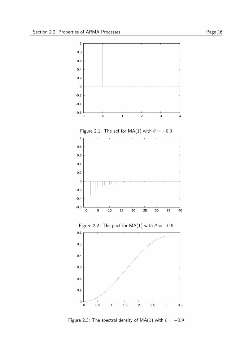
Figures 2.1 and 2.4 show the plots of the acf of Example 2.16 for θ = 0.9 and θ = −0.9respectively. The acf is zero after lag 1 in both plots and it is negative for θ = −0.9 and positivefor θ = 0.9.

Figures 2.3 and 2.6 show the plots of the spectral density of Example 2.16 for θ = 0.9 andθ = −0.9 respectively. The spectral density of Figure 2.3 is large for low frequencies, and smallfor high frequencies (for θ > 0), since the process has a large lag one positive autocorrelationas seen in Figure 2.1. Similarly, the spectral density of Figure 2.6 is negatively large for lowfrequencies since the process has a negative autocorrelation at lag one (since θ > 0) as seen inFigure 2.4.

Figure 2.7 and 2.8 show the plots of the acf and spectral density of an ARMA(2,1) process withφ1 = 0.5, φ2 = −0.4 and θ = 0.9. The spectral density is maximum at lag 1 and minimum atlag 3 since from Figure 2.7, the acf is maximum at lag 1 and minimum at lag 3.


-0.6

-0.4

-0.2

0

0.2

0.4

0.6

0.8

1

-1 0 1 2 3 4

Figure 2.1: The acf for MA(1) with θ = −0.9

-0.6

-0.4

-0.2

0

0.2

0.4

0.6

0.8

1

0 5 10 15 20 25 30 35 40

Figure 2.2: The pacf for MA(1) with θ = −0.9

0

0.1

0.2

0.3

0.4

0.5

0.6

0 0.5 1 1.5 2 2.5 3 3.5

Figure 2.3: The spectral density of MA(1) with θ = −0.9


0

0.2

0.4

0.6

0.8

1

-1 0 1 2 3 4

Figure 2.4: The acf for MA(1) with θ = 0.9

-0.4

-0.2

0

0.2

0.4

0.6

0.8

1

0 5 10 15 20 25 30 35 40

Figure 2.5: The pacf for MA(1) with θ = 0.9

0

0.1

0.2

0.3

0.4

0.5

0.6

0 0.5 1 1.5 2 2.5 3 3.5

lag

Figure 2.6: The spectral density of MA(1) with θ = 0.9


Figure 2.7: The acf of ARMA(2,1) with θ1 = 0.9, φ1 = 0.5 and φ2 = −0.4

0

0.2

0.4

0.6

0.8

1

1.2

1.4

0 0.5 1 1.5 2 2.5 3 3.5

Figure 2.8: The spectral density of ARMA(2,1) with θ1 = 0.9, φ1 = 0.5 and φ2 = −0.4

3. Prediction

In this chapter, we investigate the problem of predicting the values {Xt}t≥n+1 of a stationaryprocess in terms of {Xt}t=1,...,n.

Let {Xt} be a stationary process with E(Xt) = 0, and autocovariance function γ. Suppose wehave observations x1, x2, . . . , xn and we want to find a linear combination of x1, x2, . . . , xn thatestimates xn+1, i.e.

X̂n+1 =n∑

i=0

ΦniXi, (3.1)

such that the mean squared errorE|Xn+1 − X̂n+1|2 (3.2)

is minimized.Using the projection theorem Theorem 2.3.1 in [BD87], we can rewrite Equation (3.2) as

E

[(Xn+1 −

n∑

i=0

ΦniXi

)Xk

]= 0, ∀ k = 1, 2, . . . , n. (3.3)

From Equation (3.3), we have

E(Xn+1Xk) =

n∑

i=0

ΦniE(XkXi) (3.4)

For k = n:

E(Xn+1Xn) = γ(1) =n∑

i=0

ΦniE(XnXi) =

n∑

i=0

Φniγ(n− i), (3.5)

for k = n− 1:

E(Xn+1Xn−1) = γ(2) =

n∑

i=0

ΦniE(Xn−1Xi) =

n∑

i=0

Φniγ(n− 1 − i), (3.6)

continuing up to k = 1, we have

E(Xn+1X1) = γ(n) =

n∑

i=0

ΦniE(X1Xi) =

n∑

i=0

Φniγ(1 − i). (3.7)

Combining all the equations of the autocovariances, we have

γ(1)γ(2)

...γ(n− 1)γ(n)

=

γ(n− 1) γ(n− 2) . . . γ(1) γ(0)γ(n− 2) γ(n− 3) . . . γ(0) γ(1)

......

......

...γ(1) γ(0) . . . γ(n− 3) γ(n− 2)γ(0) γ(1) . . . γ(n− 2) γ(n− 1)

Φn1

Φn2

...Φnn−1

Φnn

(3.8)

19

Section 3.1. The Durbin-Levinson Algorithm Page 20

γn = ΓnΦn (3.9)

Due to the projection theorem, there exists a unique solution Φn if Γn is non-singular. Thisimplies Γ−1

n exists. ThereforeΦn = Γ−1

n γn. (3.10)

We use the Durbin-Levinson, a recursive method, to calculate the prediction of Xn+1.

3.1 The Durbin-Levinson Algorithm

The Durbin-levinson algorithm is a recursive method for computing Φn and vn = E|Xn − X̂n|2.Let X̂1 = 0 and

X̂n+1 =n∑

i=1

ΦniXn−i+1 n = 1, 2, . . . (3.11)

= X1Φnn+ . . .+XnΦn1

, (3.12)

and the mean squared error of prediction be defined as

vn = E(Xn+1 − X̂n+1)2, (3.13)

where v0 = E(X1)2 = γ(0). Φn = (Φn1

, . . . ,Φnn)T and vn can be calculated recursively as

follows:

Proposition 3.1 (The Durbin-Levinson Algorithm) If {Xt} is a stationary process withE(Xt) = 0 and autocovariance function γ such that γ(0) > 0 and γ(h) → 0 as h → ∞, thenthe coefficients Φni

and the mean squared errors vn given by Equations (3.12) and (3.13) satisfy

Φnn =1

vn−1

[γ(n) −

n−1∑

i=1

φn−1,iγ(n− i)

](3.14)

where

φn1...

φn,n−1

=

φn−1,1

...φn−1,n−1

− Φnn

φn−1,n−1

...φn−1,1

(3.15)

andvn = vn−1[1 − φ2

nn] (3.16)

with φ11 = γ(1)γ(0)

and v0 = γ(0).

Proof 3.2 see [BD87], Chapter 5.2.

4. Estimation of the Parameters

An appropriate ARMA(p,q) process to model an observed stationary time series is determined bythe choice of p and q and the approximate calculation of the mean, the coefficients {φj}j=1,...,p,{θi}i=1,...,q and the white noise variance σ2. In this chapter, we will assume that the data has beenadjusted by subtraction of the mean, and the problem thus transforms into fitting a zero-meanARMA model to the adjusted data {Xt}t∈Z for constant values of p and q.

4.1 The Yule-Walker Equations

Let {Xt}t∈Z be the zero-mean causal autoregressive process defined in Equation (2.3). We willnow find the estimators of the coefficient vector Φ = (φ1, . . . , φp)

T and the white noise varianceσ2 based on the observations x1, . . . , xn. We assume that {Xt}t∈Z can be expressed in the formof Equation (2.10), i.e. {Xt}t∈Z is causal.

Multiply each side of Equation (2.3) for Xt+1 by Xt, to get

XtXt+1 =

p∑

j=1

φjXtXt−j+1 +XtZt+1, (4.1)


Taking expectations, we have

E(XtXt+1) =

p∑

j=1

E (φjXtXt−j+1) + E (XtZt+1) (4.2)

=

p∑

j=1

φjE (XtXt−j+1) + E (XtZt+1) , (4.3)

E (XtZt+1) = 0 since the random noise of the future time t + 1 is uncorrelated of Xt due tocausality. Hence,

γ(1) =

p∑

j=1

φjγ(j − 1). (4.4)

To get the autocovariance at lag 2, multiply each side of Equation (2.3) by Xt−1, to get

Xt−1Xt+1 =

p∑

j=1

φjXt−1Xt−j+1 +Xt−1Zt+1, (4.5)


21

Section 4.1. The Yule-Walker Equations Page 22

Taking expectations, we have

E (Xt−1Xt+1) =

p∑

j=1

E (φjXt−1Xt−j+1) + E (Xt−1Zt+1) (4.6)

=

p∑

j=1

φjE (Xt−1Xt−j+1) + E (Xt−1Zt+1) (4.7)

γ(2) =

p∑

j=1

φjγ(j − 2). (4.8)

Continuing this process, we have the autocovariance at lag p as

γ(p) =

p∑

j=1

φjγ(j − p). (4.9)

Combining all the equations of the autocovariances

γ(1) = φ1γ(0) + φ2γ(1) + . . .+ φpγ(p− 1)

γ(2) = φ1γ(1) + φ2γ(0) + . . .+ φpγ(p− 2)... =

......

γ(p− 1) = φ1γ(p− 2) + φ2γ(p− 3) + . . .+ φpγ(1)

γ(p) = φ1γ(p− 1) + φ2γ(p− 2) + . . .+ φpγ(0)

γ(1)γ(2)

...γ(p− 1)γ(p)

=

γ(0) γ(1) . . . γ(p− 2) γ(p− 1)γ(1) γ(0) . . . γ(p− 3) γ(p− 2)

......

......

...γ(p− 2) γ(p− 3) . . . γ(0) γ(1)γ(p− 1) γ(p− 2) . . . γ(1) γ(0)

φ1

φ2...

φp−1

φp

(4.10)

orγp = ΓpΦ, (4.11)

where γ(h) = γ(−h), Γp is the covariance matrix, γp = (γ(1), . . . , γ(p))T and Φ = (φ1, . . . , φp)T .

To get the estimators for the white noise variance σ2, multiply Equation (2.3) by Xt and takeexpectations of both sides

X2t = φ1Xt−1Xt + φ2Xt−2Xt + . . .+ φpXt−pXt + ZtXt, t ∈ Z,

E(X2

t

)= φ1E (Xt−1Xt) + φ2E (Xt−2Xt) + . . .+ φpE (Xt−pXt) + E (ZtXt) .

From the causality assumption,

E(ZtXt) = E(Zt

∞∑

j=0

ψjZt−j)

=∞∑

j=0

ψjE(ZtZt−j) = σ2.

Section 4.1. The Yule-Walker Equations Page 23

Therefore,

γ(0) = φ1γ(1) + φ2γ(2) + . . .+ φpγ(p) + σ2

σ2 = γ(0) − φ1γ(1) − φ2γ(2) − . . .− φpγ(p)

σ2 = γ(0) − ΦTγp. (4.12)

Equations (4.11) and (4.12) are the Yule-Walker equations which can be used to determineγ(0), . . . , γ(p) from σ2 and Φ.

Replacing the covariances γ(j), j = 0, . . . , p in Equations (4.11) and (4.12) by the correspondingsample covariances

γ̂(j) =1

n

n−h∑

k=1

(xk+h − x)(xk − x), 0 < h ≤ n, (4.13)

andγ̂(h) = γ̂(−h), −n < h ≤ 0, (4.14)

where x = 1n

n∑

k=1

xk is the sample mean of the sample {xk}k=0,...,n. We obtain a set of equations

for the Yule-Walker estimators Φ̂ and σ̂2, of Φ and σ2, respectively

Γ̂pΦ̂ = γp, (4.15)

andσ̂2 = γ̂(0) − Φ̂T γ̂p. (4.16)

Dividing Equation (4.15) by γ̂(0), we have

R̂pΦ̂ = ρ̂p, (4.17)

where R̂p =bΓp

bγ(0)and R̂p = R̂T

p since R̂p is a symmetric matrix. R̂p has a non-zero determinant

if γ̂(0) > 0 ([BD87], Chapter 5.1). Hence from Equation (4.17),

Φ̂ = R̂−1p ρ̂p. (4.18)

Substituting Equation (4.18) into Equation (4.16), we have

σ̂2 = γ̂(0) − (R̂−1p ρ̂p)

T γ̂p = γ̂(0)(1 − ρ̂T

p R̂−1p ρ̂p

). (4.19)

From Equation (4.17), we have 1− φ̂1z− . . .− φ̂pzp 6= 0 for |z| < 1. Therefore, the fitted model

Xt − φ̂1Xt−1 − . . .− φ̂pXt−p = Zt {Zt},∼WN(0, σ̂2) (4.20)

is causal. The autocovariances γF (h), h = 0, . . . , p, of the fitted model therefore satisfy the p+1linear equations

γF (h) − φ̂1γF (h− 1) − . . .− φ̂pγF (h− p) =

{0, h = 1, . . . , p,

σ̂2, h = 0.(4.21)

From Equations (4.15) and (4.16) we have γF (h) = γ̂(h), h = 0, 1, . . . , p. This implies that theautocovariances of the fitted model at lags 0, 1, . . . , p coincide with the sample autocovariances.

Section 4.2. The Durbin-Levinson Algorithm Page 24

Theorem 4.1 If {Xt} is the causal AR(p) process defined by Equation (2.3) with {Zt} ∼IID(0, σ2), and if Φ̂ = (φ̂1, . . . , φ̂p). Then

√n(Φ̂ − Φ)

d→ N(0, σ2Γ−1p ), n→ ∞, (4.22)

where Γp = (γ(i − j))i,j=1,...,p is the (unknown) true covariance matrix, N(0, σ) is the normal

distribution with zero mean and variance σ andd→ denotes convergence in distribution. Further-

more,σ̂2 p→ σ2, n→ ∞

in probability.

Proof 4.2 See [BD87], Chapter 8.10.

Remark 4.3 We can extend the idea leading to the Yule-Walker equations to general ARMA(p,q)process. However, the estimates for φ1, . . . , φp, θ1, . . . , θq, σ

2 are not consistent i.e. Theorem 4.1does not hold anymore. One usually uses the Yule-Walker estimates as starting values in MaximumLikelihood Estimation.

4.2 The Durbin-Levinson Algorithm

Levinson and Durbin derived an iterative way of solving the Yule-Walker equations (see Section

3.1). Instead of solving (4.11) and (4.12) directly, which involves inversion of R̂p, the Levinson-Durbin algorithm fits AR models of successively increasing orders AR(1), AR(2), . . . , AR(p) tothe data. The fitted AR(m) process is then given by

Xt − φ̂m1Xt−1 − . . .− φ̂mmXt−m, {Zt} ∼WN(0, σ̂m), (4.23)

where from Equations (4.18) and (4.19)

Φ̂m = (φ̂m1, . . . , φmm) = R̂−1p ρ̂m, (4.24)

andσ̂m = γ̂(0)

(1 − ρ̂T

mR̂−1m ρ̂m

). (4.25)

Proposition 4.4 If γ̂(0) > 0 then the fitted AR(m) model in Equation (4.24) for m = 1, 2, . . . , pis recursively calculated from the relations

φ̂mm =1

σ̂m−1

[

γ̂(m) −m−1∑

j=1

φ̂m−1,jγ̂(m− j)

]

, (4.26)

φ̂m1

...

φ̂m,m−1

= Φ̂m−1 − φ̂mm

φ̂m−1,m−1

...

φ̂m−1,1

(4.27)

Section 4.3. The Innovations Algorithm Page 25

andσ̂m = σ̂m−1(1 − φ̂2

mm), (4.28)

with φ̂11 = ρ̂(1) and σ̂1 = γ̂(0)[1 − ρ̂2(1)].

Definition 4.5 For n ≥ 2, α(n) = Φnn is called the partial autocorrelation function. For n = 1,α(1) = ρ(1) = cor(Xt, Xt+1). α(n) measures the correlation between Xt and Xt+n taking intoaccount the observations Xt+1, . . . , Xt+n−1 lying in between.

Proposition 4.6 For an AR(p) model, the partial autocorrelation is zero after lag p, i.e. α(h) =0, ∀ h > p and for a MA(q) model, α(h) 6= 0 ∀ h.

Example 4.7 Given that a time series has sample autocovariances γ̂(0) = 1382.2, γ̂(1) =1114.4, γ̂(2) = 591.73, and γ̂(3) = 96.216 and sample autocorrelations ρ̂(0) = 1, ρ̂(1) =0.8062, ρ̂(2) = 0.4281, and ρ̂(3) = −0.0.696, we use the Durbin-Levinson algorithm to find theparameters φ1, φ2, and σ2 in the AR(2) model,

Yt = φ1Yt−1 + φ2Yt−2 + Zt, {Zt} ∼WN(0, σ2), (4.29)

where Yt = Xt−46.93 is the mean-corrected series. We calculate φ1, φ2, and σ2 from Proposition4.4 as follows:

φ̂11 = ρ̂(1) = 0.8062

σ̂1 = γ̂(0)(1 − ρ̂21) = 1382.2(1 − 0.80622) = 483.83

φ̂22 =1

σ̂1

(γ̂(2) − φ̂11γ̂(1)) =1

483.82(591.73 − 0.8062 · 1114.4) = −0.6339

φ̂21 = φ̂11 − φ̂22φ̂11 = 0.8062 + 0.6339 · 0.8062 = 1.31725

σ̂2 = σ̂1(1 − φ̂22) = 483.82(1 − (−0.6339)2) = 289.4.

Hence the fitted model is

Yt = 1.31725Yt−1 − 0.6339Yt−2 + Zt, {Zt} ∼WN(0, 289.4)

Therefore, the model for the original series {Xt} is

Xt = 46.93 + 1.31725(Xt−1 − 46.93) − 0.6339(Xt−2 − 46.93) + Zt

= 14.86 + 1.31725Xt−1 − 0.6339Xt−2 + Zt, {Zt} ∼WN(0, 289.4)

4.3 The Innovations Algorithm

We fit a moving average model

Xt = Zt + θ̂m1Zt−1 + . . .+ θ̂mmZt−m, {Zt} ∼ WN(0, v̂m) (4.30)

of orders m = 1, 2, . . . q by means of the Innovations algorithm just as we fit AR models of orders1, 2, . . . , p to the data x1, . . . , xn by the Durbin-Levinson algorithm.

Section 4.3. The Innovations Algorithm Page 26

Definition 4.8 If γ̂(0) > 0 then the fitted MA(m) model in Equation (4.30) for m = 1, 2, . . . , q,can be determined recursively from the relations

θ̂m,m−k =1

v̂k

[γ̂(m− k) −

k−1∑

j=0

θ̂m,m−j θ̂k,k−j v̂j

], k = 0, . . . , q, (4.31)

and

v̂m = γ̂(0) −k−1∑

j=0

θ̂2m,m−j v̂j (4.32)

where v0 = γ̂(0).

Remark 4.9 The estimators θ̂q1, . . . , θ̂qq, obtained by the Innovations algorithm are usually notconsistent in contrast to the Yule-Walker estimates. For MA(q) as well as for general ARMA(p,q)process, one therefore uses Maximum Likelihood Estimation (MLE) techniques which we will notintroduce in this essay. We refer to [BD87], Chapter 8.7 for details on MLE.

5. Data Example

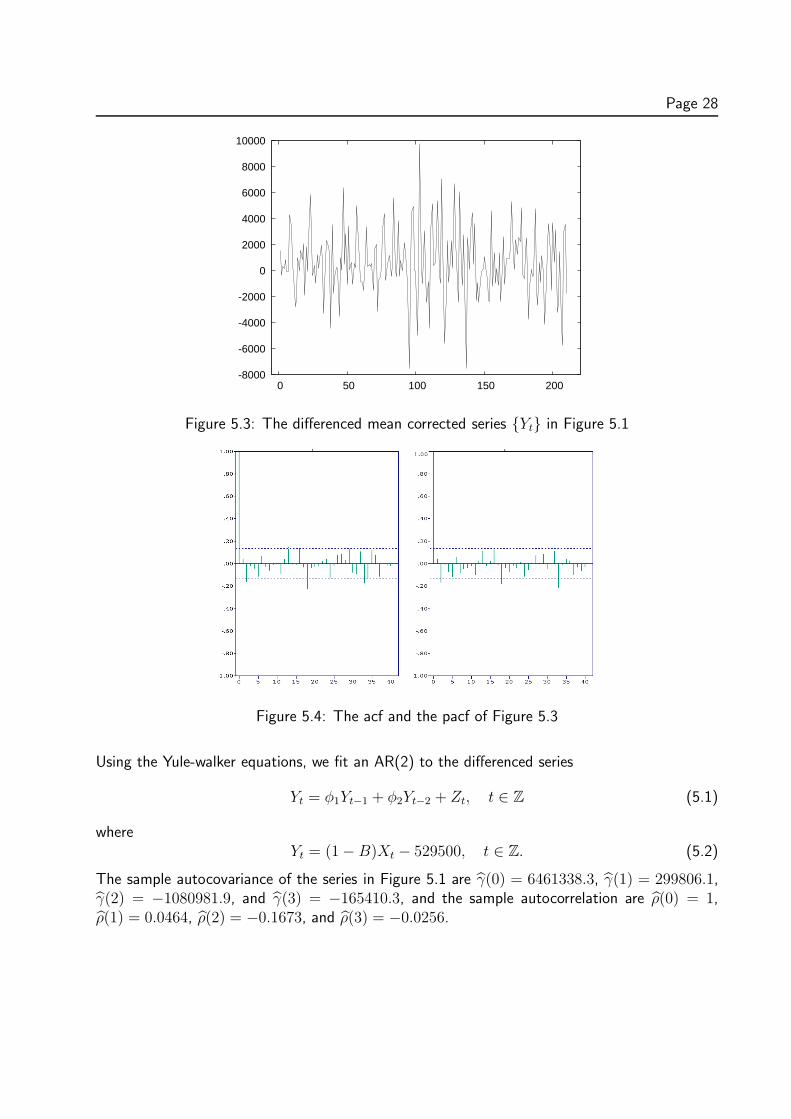
Figure 5.1 shows the plot of the values of the SP500 index from January 3, 1995 to October 31,1995 (Source: Hyndman, R. J. (n.d.) Time Series Data Library. Accessed on May 20, 2007).The series {Xt} shows an overall upward trend, hence it is non-stationary. Figure 5.2 gives theplot of the autocorrelation and the partial autocorrelation of the series in Figure 5.1. The slowdecay of the acf is due to the upward trend in the series. This suggests differencing at lag 1, i.e.we apply the operator (1 − B) (see Chapter 1.3). The differenced series produces a new seriesshown in Figure 5.3. From the graph, we can see that the series is stationary. Figure 5.4 showsthe plot of the autocorrelation function and the partial autocorrelation function of the differenceddata which suggests fitting an autoregressive average model of order 2 (see Proposition 4.6).

440000

460000

480000

500000

520000

540000

560000

580000

600000

0 50 100 150 200 250

Figure 5.1: The plot of the original series {Xt} of the SP500 index

Figure 5.2: The acf and the pacf of Figure 5.1

27

Page 28

-8000

-6000

-4000

-2000

0

2000

4000

6000

8000

10000

0 50 100 150 200

Figure 5.3: The differenced mean corrected series {Yt} in Figure 5.1

Figure 5.4: The acf and the pacf of Figure 5.3

Using the Yule-walker equations, we fit an AR(2) to the differenced series

Yt = φ1Yt−1 + φ2Yt−2 + Zt, t ∈ Z (5.1)

whereYt = (1 − B)Xt − 529500, t ∈ Z. (5.2)

The sample autocovariance of the series in Figure 5.1 are γ̂(0) = 6461338.3, γ̂(1) = 299806.1,γ̂(2) = −1080981.9, and γ̂(3) = −165410.3, and the sample autocorrelation are ρ̂(0) = 1,ρ̂(1) = 0.0464, ρ̂(2) = −0.1673, and ρ̂(3) = −0.0256.

Page 29

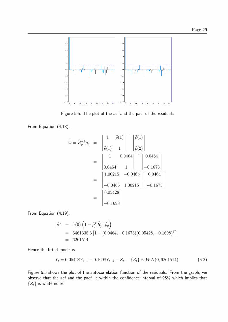
Figure 5.5: The plot of the acf and the pacf of the residuals


Φ̂ = R̂−1p ρ̂p =

1 ρ̂(1)

ρ̂(1) 1

−1

ρ̂(1)

ρ̂(2)

=

1 0.0464

0.0464 1

−1

0.0464

−0.1673

=

1.00215 −0.0465

−0.0465 1.00215

0.0464

−0.1673

=

0.05428

−0.1698


σ̂2 = γ̂(0)(1 − ρ̂T

p R̂−1p ρ̂p

)

= 6461338.3[1 − (0.0464,−0.1673)(0.05428,−0.1698)T

]

= 6261514

Hence the fitted model is

Yt = 0.05428Yt−1 − 0.1698Yt−2 + Zt, {Zt} ∼WN(0, 6261514). (5.3)

Figure 5.5 shows the plot of the autocorrelation function of the residuals. From the graph, weobserve that the acf and the pacf lie within the confidence interval of 95% which implies that{Zt} is white noise.

Page 30

Figure 5.6: The spectral density of the fitted model

Figure 5.7: The plot of the forecasted values with 95% confidence interval

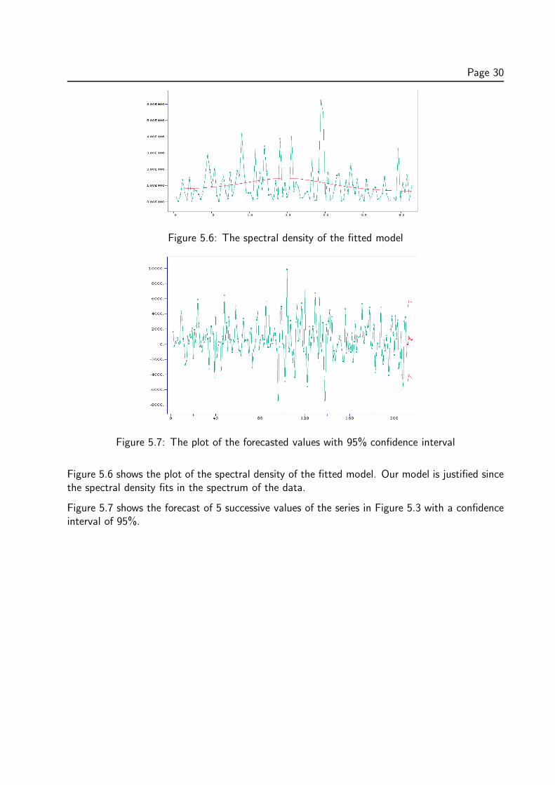
Figure 5.6 shows the plot of the spectral density of the fitted model. Our model is justified sincethe spectral density fits in the spectrum of the data.

Figure 5.7 shows the forecast of 5 successive values of the series in Figure 5.3 with a confidenceinterval of 95%.

6. Conclusion

This essay highlighted the main features of time series analysis. We first introduced the basicideas of time series analysis and in particular the important concepts of stationary models and theautocovariance function in order to gain insight into the dependence between the observationsof the series. Stationary processes play a very important role in the analysis of time series anddue to the non-stationary nature of most data, we discussed briefly a method for transformingnon-stationary series to stationary ones.

We reviewed the general autoregressive moving average (ARMA) processes, an important classof time series models defined in terms of linear difference equations with constant coefficients.ARMA processes play an important role in modelling time-series data. The linear structure ofARMA processes leads to a very simple theory of linear prediction which we discussed in Chapter3. We used the observations taken at or before time n to forecast the subsequent behaviour ofXn.

We further discussed the problem of fitting a suitable AR model to an observed discrete time seriesusing the Yule-Walker equations. The major diagnostic tool used is the sample autocorrelationfunction (acf) discussed in Chapter 1. We illustrated with a data example, the process of fittinga suitable model to the observed series and estimated its paramters. From our estimation, wefitted an autoregressive process of order 2 and with the fitted model, we predicted the next fiveobservations of the series.

This essay leaves room for further study of other methods of forecasting and estimation ofparameters. Particularly interesting are the Maximum Likelihood Estimators for ARMA processes.

31

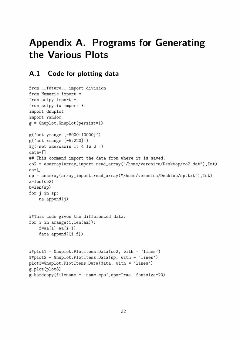
Appendix A. Programs for Generatingthe Various Plots

A.1 Code for plotting data

from __future__ import division

from Numeric import *

from scipy import *

from scipy.io import *

import Gnuplot

import random

g = Gnuplot.Gnuplot(persist=1)

g(’set yrange [-8000:10000]’)

g(’set xrange [-5:220]’)

#g(’set xzeroaxis lt 4 lw 2 ’)

data=[]

## This command import the data from where it is saved.

co2 = asarray(array_import.read_array("/home/veronica/Desktop/co2.dat"),Int)

aa=[]

sp = asarray(array_import.read_array("/home/veronica/Desktop/sp.txt"),Int)

a=len(co2)

b=len(sp)

for j in sp:

aa.append(j)

##This code gives the differenced data.

for i in arange(1,len(aa)):

f=aa[i]-aa[i-1]

data.append([i,f])

##plot1 = Gnuplot.PlotItems.Data(co2, with = ’lines’)

##plot2 = Gnuplot.PlotItems.Data(sp, with = ’lines’)

plot3=Gnuplot.PlotItems.Data(data, with = ’lines’)

g.plot(plot3)

g.hardcopy(filename = ’name.eps’,eps=True, fontsize=20)

32

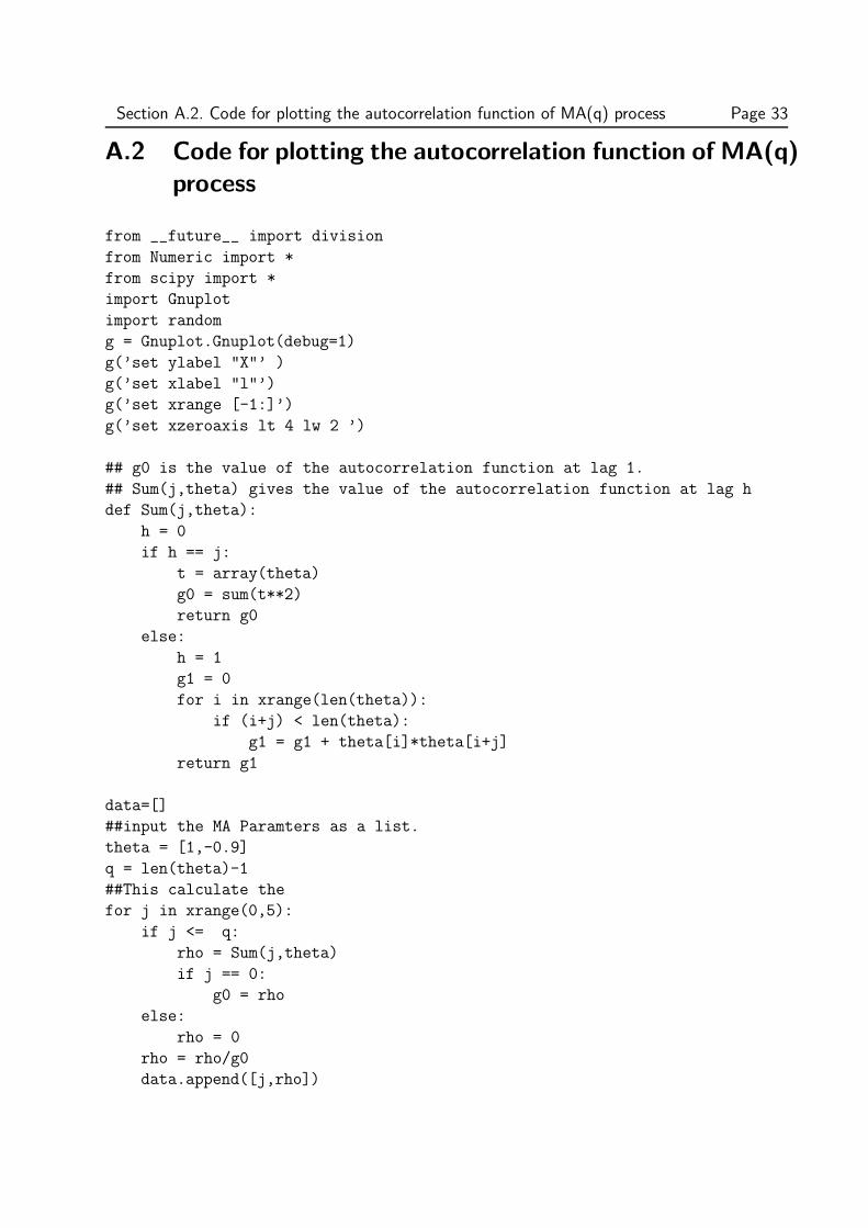
Section A.2. Code for plotting the autocorrelation function of MA(q) process Page 33

A.2 Code for plotting the autocorrelation function of MA(q)

process



from scipy import *

import Gnuplot

import random

g = Gnuplot.Gnuplot(debug=1)

g(’set ylabel "X"’ )

g(’set xlabel "l"’)

g(’set xrange [-1:]’)

g(’set xzeroaxis lt 4 lw 2 ’)

## g0 is the value of the autocorrelation function at lag 1.

## Sum(j,theta) gives the value of the autocorrelation function at lag h

def Sum(j,theta):

h = 0

if h == j:

t = array(theta)

g0 = sum(t**2)

return g0

else:

h = 1

g1 = 0

for i in xrange(len(theta)):

if (i+j) < len(theta):

g1 = g1 + theta[i]*theta[i+j]

return g1

data=[]

##input the MA Paramters as a list.

theta = [1,-0.9]

q = len(theta)-1

##This calculate the

for j in xrange(0,5):

if j <= q:

rho = Sum(j,theta)

if j == 0:

g0 = rho

else:

rho = 0

rho = rho/g0

data.append([j,rho])

Section A.3. Code for plotting the partial autocorrelation function of MA(1) process Page 34

plot1 = Gnuplot.PlotItems.Data(data, with = ’impulses’)

g.plot(plot1)

#g.hardcopy()


A.3 Code for plotting the partial autocorrelation function

of MA(1) process



from scipy import *

import Gnuplot

import random

g = Gnuplot.Gnuplot(debug=1)

##g(’set terminal png’)


g(’set xlabel "l"’)

g(’set xrange [-1:]’)

g(’set xzeroaxis lt 4 lw 2 ’)

data=[]

theta=0.9

for k in arange(0,40):

if k == 0:

alpha = 1

else:

alpha =- (-theta)**k*(1-theta**2)/(1-theta**(2*(k+1)))

data.append([k,alpha])

plot1 = Gnuplot.PlotItems.Data(data, with = ’impulses’)

g.plot(plot1)


A.4 Code for Plotting the Spectral Density Function of

MA(1) process



Section A.4. Code for Plotting the Spectral Density Function of MA(1) process Page 35

from scipy import *

import Gnuplot

import random

g = Gnuplot.Gnuplot(persist=1)


g(’set xlabel "lag"’)

data=[]

specify the value of theta

theta=

for l in arange(0, pi+pi/13, pi/18):

f = 1/(2*pi)*(1+theta**2-2*theta*cos(l))

data.append([l,f])

plot1 = Gnuplot.PlotItems.Data(data, with = ’lines’)#, title = ’plot’)

g.plot(plot1)


Acknowledgements

To GOD be the GLORY.

I express my profound gratitude to my supervisor, Dr. Tina Marie Marquardt, for her help andproviding many suggestions, guidance, comments and supervision at all stages of this essay. Iexpress my indebtedness to Prof. F. K. Allotey, Prof. Francis Benya and staff of the Departmentof Mathematics, KNUST, for their support and advice.

Many thanks to AIMS staff and tutors for the knowledge I have learned from them. Without thehelp of my colleagues especially my best friends Mr. Wole Solana, Miss. Victoria Nwosu and Mr.Jonah Emmanuel Ohieku, my wonderful brothers Mr. Henry Amuasi, Mr. Samuel Nartey andMr. Eric Okyere, my stay at AIMS would not have been a successful one. I am very grateful fortheir support.

I would not forget to appreciate my family for their help, love and support throughout myeducation.

GOD BLESS YOU ALL.

36

Bibliography

[BD87] P. J. Brockwell and R. A. Davis, Time series: Theory and methods, Springer-Verlag,1987.

[BD02] P. J. Brockwell and R. A. Davis, Introduction to time series and forecasting, 2nd ed.,Spinger-Verlag, New York, 2002.

[Cha01] C. Chatfield, Time series forecasting, sixth ed., Chapman and Hall/CRC, New York,2001.

[Cha04] C. Chatfield, The analysis of time series: An introduction, Chapman and Hall/CRC,New York, 2004.

37

Documents

Discrete Time Series Analysis With ARMA Models